Forthcoming

Journal of Comparative Economics

Does Reform Work?

An Econometric Survey of the Reform-Growth Puzzle

Jan Babecký

Czech National Bank

and University of Paris-1 Sorbonne

Nauro F. Campos**

Brunel University,

CEPR and IZA

October 2010

Abstract: There is still an intense controversy about the empirical support

for the effects of structural reforms on economic growth. This paper uses

data from 46 studies and more than 500 estimates to (a) document the

variation in these estimated effects and (b) identify the main factors that help

explain it. We put forward evidence, based on the general-to-specific

method, suggesting that the estimated long-run effects of reform on growth

are normally distributed, and that accounting for institutions and initial

conditions (trade liberalization) are principal factors in decreasing

(increasing) the probability of reporting significant and positive effects of

reform on growth.

JEL Classification: O11, P21, C49

Keywords: Growth, liberalization, structural reforms, transition economies

* We thank Daniel Berkowitz (the Editor), Fabrizio Coricelli, Balazs Egert, Jan Fidrmuc, Jarko

Fidrmuc, Laszlo Halpern, Jan Hanousek, Roman Horvath, Evzen Kocenda, Iikka Korhonen,

Tomasz Mickiewicz, Bilin Neyapti, Richard Pomfret, Karsten Staehr, Tom Stanley, Johan

Swinnen, Jan Visek, two anonymous referees and seminar participants at the Czech National

Bank, Czech Economic Society, European Bank for Reconstruction and Development (EBRD),

Western Economic Association (San Diego) and European Econometric Society (Vienna) for

valuable comments on previous versions. Evgeny Plaksen, Dana Popa and Ekaterina

Shironosova provided superb research assistance. Campos is grateful for financial support from

the Economic and Social Research Council (ESRC), Research Grant RES-000-22-0550. All

remaining errors are entirely our own.

** Corresponding author: Department of Economics, Brunel University, London, UB8 3PH,

United Kingdom. Fax: + 44 1895 269 770, E-mail: nauro.campos@brunel.ac.uk

1

1. Introduction

Arguably, one of the most heated debates of the last two decades has been on the

macroeconomic implications of structural reforms, or more specifically, on the economic

growth pay-offs one should observe from the implementation of such reforms. Since the late

1980s, a large number of structural reform programmes were designed and implemented across

the world, with varying degrees of success. The reasons underlying this variation are still

largely unknown and raise a number of questions. Does reform work? What do we know in

terms of the evaluation of those reform efforts? Did the expected growth and welfare dividends

occur? How robust are the available econometric estimates of the growth pay-offs of structural

reforms? What are the main factors that help explain their variation? Is the variation driven by

measurement and data quality issues, by the diversity of underlying theoretical frameworks, or

by differences in econometric methodology?

The objective of this paper is to take stock of the econometric evidence on the impact of

structural reforms on economic growth, with emphasis on the experience of the transition

economies. We put together a data set covering more than 500 estimates of the effect of

reforms on growth (collected from 46 studies, listed in Appendix 1) separated according to

their cumulative (or long-term) and contemporaneous (or short-run) nature. How large is the

variation of these estimates? Figures 1 to 3 show plots of their t-statistics: for all estimates and

then for only contemporaneous and only cumulative, respectively. First note that, somewhat

unsurprisingly, the short-run effect tends to be negative while the long-run effect tends to be

positive. Moreover, the cumulative effect is the only case for which we can not reject the

hypothesis that the estimates of the reform effects on growth follow the normal distribution.1

The variation of the contemporaneous effects is also remarkable, with the average short-run

1 Applying the aggregate t-statistics method suggested by Djankov and Murrell (2002) reveals that there

is a genuine positive and statistically significant long-term effect of reform on growth (full details are

below).

2

effect being negative. The extent of variation of the estimated impacts of structural reforms on

economic growth, as so clearly revealed by these Figures, suggests that this is fertile ground for

meta-regression analysis.

Meta-regression analysis (hereafter, MRA) is a statistical methodology that provides a

summary as well as a quantitative assessment of a given body of evidence (Stanley, 2001;

Stanley and Jarrell, 1989). In a typical MRA study, the dependent variable is a summary

statistic (for instance, elasticities or t-values) while the independent variables reflect various

features of the econometric strategy and data used in each study. MRA has been widely used in

economics. In environmental economics, Florax (2002) reviews 40 meta-regression studies

(mostly on pollution valuation) published since 1980. It has also been used extensively in

labour economics: Card and Krueger (1995) use MRA to assess the evidence on minimum

wages, Stanley and Jarrell (1998) use it to evaluate that on gender wage differentials in the

United States, while Ashenfelter et al. (1999) use it to investigate the evidence on returns to

education.2 In international macroeconomics, Rose and Stanley (2005) use MRA to evaluate

the evidence on the effects of currency unions on international trade, Fidrmuc and Korhonen

(2006) to assess that on business cycle synchronization, and Égert and Halpern (2006) to

appraise the findings on equilibrium exchange rates.

In this paper, we apply MRA to the econometric evidence on structural reforms and

economic growth.3 MRA complements rather naturally a long and important stream of

evaluative work in the growth literature of which Levine and Renelt (1992) is one seminal

contribution (see also Durlauf et al., 2005). While the objective of most of this work is to

2 Jarrell and Stanley (1990) use MRA to evaluate the evidence on the union/non-union wage gap,

Weichselbaumer and Winter-Ebmer (2001) to assess that on gender wage differentials across countries,

and Doucouliagos (1995) uses it to take stock of the econometric evidence on worker participation. In

public finance, MRA has been used to assess the impact of tax policies (Phillips and Goss, 1995) and to

evaluate econometric findings on the Ricardian equivalence (Stanley, 1998). 3 In comparative economics, Djankov and Murrell (2002) use MRA to assess the empirical evidence on

enterprise restructuring. Havrylyshyn (2001) provides a review of the relationship between reform and

growth but we are unaware of any MRA study focusing on the issue.

3

establish which variables are more or less robustly related to economic growth, MRA throws

light on the main reasons why a given variable (or set of variables) is more or less robustly

related to economic growth.

The data set we put together for this paper is based on information hand-collected from

46 econometric studies, covering a total of approximately 520 estimates of the effect of reform

on growth. We quantified more than 40 features of those studies encompassing estimation

method, measurement, specification and quality (Appendix 2 provides the full list of variables).

We investigate both the contemporaneous (short-term) and cumulative (long-term) effect of

reform on economic performance. In addition to different types of reform effects, the paper

uses a general-to-specific strategy to try to get at the reasons for the variation in the effect of

structural reform on economic growth we observe (Figures 1-3), taking into account both

publication bias and perceived differences in the quality of the papers. There is wide agreement

(the few minor divergences are discussed in detail below) from the results of the general-to-

specific and method-measurement-specification strategies.

Our main findings are that accounting for institutions and initial conditions are two main

factors in decreasing the probability of reporting significant and positive effects of reform on

growth, while focusing solely on trade liberalization significantly increases this probability.

We also find that authors‟ affiliation matters: academic authors systematically tend to report

smaller effects of reform on growth than authors in think-thanks, government institutes and

international organizations. Other noteworthy results include that more influential papers

(measured either by a dummy variable on whether it was published in a refereed journal or by

Google Scholar citations), papers that do not use country-specific dummy variables (fixed

effects) and with less degrees of freedom, tend to report smaller (or more negative) effects of

reform on growth. We also find interesting differences among the variables that explain the

variation in the long-run or cumulative vis-à-vis those for the contemporaneous or short-run

4

effects. In particular, we find that reform in the form of external liberalization still plays a

significant yet not as prominent a role in the short- as it does in the long-run case. Our results

suggest that this is because in the former case the impact of macroeconomic stabilization seems

to dominate.

It is also important to note at the outset that this paper focuses on a particular body of

econometric evidence on the growth-reform nexus, namely that covering the experience of the

transition economies. This focus is justified by at least four reasons: (1) this is a group of

countries for which there is a sufficiently large number of published econometric studies;4 (2)

these economies provide an almost natural experiment setting for the question at hand as they

started out with rather similar initial conditions but experienced very dissimilar reform and

growth trajectories (with some implementing reform packages in an unprecedented scale while

other being more restrictive); (3) this body of evidence tends to use similar measures of

reform5 as well as growth figures which attenuates one potentially crucial source of bias; and

(4) the studies tend to use somewhat similar econometric specifications, estimation strategies

and sets of explanatory variables.

The rest of the paper is organised as follows. The next section describes the

methodological framework. Section 3 presents the data set put together for this paper. Section

4 discusses the econometric approach and main findings, while Section 5 concludes with

suggestions for future research.

4 Acemoglu et al. (2005) note that the empirical evidence on reform-growth is still scarce, with even

that for the OECD countries being limited to a handful of papers. 5 This implies that the reform data used in the empirical literature is almost uniformly the same, and it

does not imply that we see these measures as error-free. Campos and Coricelli argue: “more emphasis

should be placed upon a better understanding of the role of economic reforms and reform strategies in

dictating the path of the transition process (…) There are a number of theoretical models that stress the

role of reform strategies. Yet the data for discriminating among these models is lacking. The few

indicators available are unnecessarily subjective (…)” (2002, p. 831).

5

2. Methodological Framework

Meta-analysis refers to a set of statistical methods for rigorously reviewing and evaluating a

body of empirical evidence. When a large number of studies have been carried out on a given

topic, combining their results in a systematic manner can provide additional strength, further

insights and greater explanatory power than can the more informal, narrative discussions of

individual results which is characteristic of traditional literature surveys. MRA goes beyond

what is often called vote-counting or head-counting (Light and Smith, 1997), in which

inference that a specific result occurs in a majority of cases is usually taken as evidence of the

significance and magnitude of the “true” effect. Head-counting is clearly neither systematic nor

statistically powerful in drawing conclusions about the findings from a body of evidence.

When the number of existing studies is very large, head-counting is even more likely to

support misleading conclusions because the Type-II errors of the individual studies do not

cancel out, but are said to add up instead (Florax et al., 2002).

One of the first procedures to summarise findings from a given body of evidence was

developed by Fischer (1932).6 It is well-known that the Fischer test is generous in ascribing

significance. Stanley and Jarrell (1998) discuss three potential reasons. First, it does not

distinguish between positive and negative statistically significant effects, as both are only

counted as significant. Second, the null hypothesis of the Fischer test is that none of the

observations reflects a genuine effect. A finding of significance therefore does not necessarily

mean that the average effect is statistically significant. Third, the assumption of unbiased

estimates is often violated for non-experimental evidence.

The technique stressing the magnitude of the effect or the “effect size” was developed by

6 It assumes that the underlying p-values are uniformly distributed under the null hypothesis of no

effect, and then proposes that minus twice the sum of the logs of the p-values follows a chi-square

distribution. This approach also assumes independence across studies and that each one of them is

unbiased; this is clearly an important assumption which is usually addressed by estimating MRA

equations with study fixed-effects so as to capture unobserved heterogeneity among findings.

6

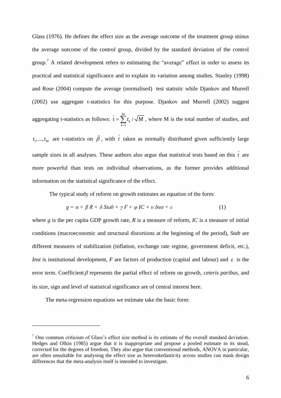
Glass (1976). He defines the effect size as the average outcome of the treatment group minus

the average outcome of the control group, divided by the standard deviation of the control

group.7 A related development refers to estimating the “average” effect in order to assess its

practical and statistical significance and to explain its variation among studies. Stanley (1998)

and Rose (2004) compute the average (normalised) test statistic while Djankov and Murrell

(2002) use aggregate t-statistics for this purpose. Djankov and Murrell (2002) suggest

aggregating t-statistics as follows: 1

/M

k

k

t t M

, where M is the total number of studies, and

1,..., Mt t are t-statistics on ̂ , with t taken as normally distributed given sufficiently large

sample sizes in all analyses. These authors also argue that statistical tests based on this t are

more powerful than tests on individual observations, as the former provides additional

information on the statistical significance of the effect.

The typical study of reform on growth estimates an equation of the form:

g = α + β R + δ Stab + γ F + φ IC + υ Inst + ε (1)

where g is the per capita GDP growth rate, R is a measure of reform, IC is a measure of initial

conditions (macroeconomic and structural distortions at the beginning of the period), Stab are

different measures of stabilization (inflation, exchange rate regime, government deficit, etc.),

Inst is institutional development, F are factors of production (capital and labour) and is the

error term. Coefficient represents the partial effect of reform on growth, ceteris paribus, and

its size, sign and level of statistical significance are of central interest here.

The meta-regression equations we estimate take the basic form:

7 One common criticism of Glass‟s effect size method is its estimate of the overall standard deviation.

Hedges and Olkin (1985) argue that it is inappropriate and propose a pooled estimate in its stead,

corrected for the degrees of freedom. They also argue that conventional methods, ANOVA in particular,

are often unsuitable for analysing the effect size as heteroskedasticity across studies can mask design

differences that the meta-analysis itself is intended to investigate.

7

i

K

k

kiki ZY 1

0 (2)

where iY is the value of summary measure in regression i, i=1…M, where M is the number of

estimates from the empirical literature (listed in Appendix 1), kiZ is a vector of K study

characteristics (following the method-measurement-specification scheme detailed in Appendix

2), and k is a vector of meta-regression coefficients which reflect the effect of particular

characteristics of the original study on the reform effect. It is common practice to use estimated

coefficients or the results of statistical tests (e.g., t-statistics) as the summary measure. In light

of the very large variation in the results from this body of evidence (Figures 1-3), the results

we report are for t-statistics.

One important feature of the literature on the effects of reform on growth is that different

studies specify different types of effects of reform on growth and, in addition, use different

measures of stabilization, initial conditions and institutional development. Thus combining the

estimated effects of interest has to be done carefully. We must be clear about which types of

reform effects are entering into the meta-analysis. A typical equation capturing the effect of

reforms on growth estimated on a panel is:

git = α + β (R it - R it-1) + δ R it-1+ γ Z it + εit (3)

where g is the measure of growth; R is the measure of the level of some policy (e.g. external

liberalization) and the Z's are a set of control variables. A formally equivalent equation is:

git = α + β Rit + δ R it-1+ γ Z it + εit (4)

where the coefficients on the initial level of reform of (3) are not the same as those of (4), and

of course neither are the β‟s. Notice that some papers estimate a form that is not equivalent to

either (1) or (2):

git = α + β Rit + γ Z it + εit (5)

where again the β‟s is a different parameter from the ones above. In the present paper, we focus

8

on long-term effects of reform and as such we focus on the coefficients δ from (3), δ plus β

from (4) and β from (5). There is also one additional possibility which although found in

empirical studies have been excluded from the present paper because it focuses on the

immediate impacts of reform. That is when the reported specification is run on a cross-section

which does not take into account the initial level of reform. These estimated effects, a minority

in the empirical literature, are excluded from our analysis. Notice that it is often the case that

the same paper presents sets of results that are included in our analysis as well as results which

we exclude from our analysis because of the sole focus on the immediate effect.

One important issue to be dealt with concerns the so-called “file drawer” problem or

publication bias. Namely, the tendency of academic journals to favour studies that report

statistically significant results. Card and Krueger (1995) and Ashenfelter et al. (1999) address

such type of publication bias in their studies of minimum wage and returns to schooling,

respectively (for a review, see Stanley, 2005). One potential difficulty is the implicit

assumption that working papers are not published (and may never be) because they do not

contain a sufficient number of statistically significant results. The fact that the literature on

reform and growth is more recent (than, for instance, on the minimum wage and returns to

education) may be in part responsible for our findings of such type of bias not being severe.8

3. Data Set

The starting point in MRA is a search for the appropriate literature from which the

observations (in this case, coefficients on the effects of reform) will be retrieved. Papers are

8 We tested for publication bias following the funnel asymmetry test–precision effect test (FAT–PET)

discussed in Stanley (2005), according to which severe publication bias is said to be absent if the plot of

the estimated effect against its precision resembles an inverse funnel and in the regression of the effect

on its precision the slope coefficient is not statistically different from zero. For our data we find that

publication bias is not a concern in the case of either contemporaneous or cumulative effects; however,

the true impact of reforms on growth is zero for the contemporaneous effect and positive and significant

for the cumulative effect. These results are available upon request.

9

included if they investigate the effect of reform on growth across transition countries, if they

clearly report the estimated coefficients of interest, if their estimates are from regression

analysis, and if their t-values or standard errors are reported in full. We find 46 papers (listed in

Appendix 1) which fulfil these criteria and use them as the basis for our data set.

We follow, among others, Weichselbaumer and Winter-Ebmer (2007) and include all

reported test statistics from each study in our meta-regression analysis. There is no consensus

on whether to choose one estimate from each study or all of the reported estimates (that is,

from all specifications reported in the original paper). Stanley (2001) argues that there are

benefits in choosing only one estimate – the one the author of the study indicate to be her

preferred one. Alternatively, Ashenfelter et al. (1999) and Weichselbaumer and Winter-Ebmer

(2007) include all the reported estimates to make full use of the existing information and to

avoid any eventually arbitrary judgement on the authors‟ preferred results.9 Here we choose to

use all the reported coefficients, but as a robustness exercise we re-run all our results adding a

set of study-specific dummy variables. This is because in this literature the authors seldom

indicate which one is their preferred estimate.

There are various possible strategies for the construction of our dependent variable. Our

strategy follows the rule of not having more than one coefficient from each reported regression.

This implies that if both contemporaneous and lagged effects of reform on growth are present

in the specification, then we only select the one on the contemporaneous effect. By the same

token, if several alternative measures of reform are used, the default is to use the most

significant coefficient (larger t-value).

For each of the 46 papers, the estimates of reform on growth and their corresponding

meta-independent variables were collected. This procedure gave one observation in our data set

9 Djankov and Murrell (2002) and Stanley and Jarrell (1998) collect multiple estimates from the same

study only if the estimates are derived from conceptually distinct analyses, i.e. different forms of the

dependent variable from different countries or from different years.

10

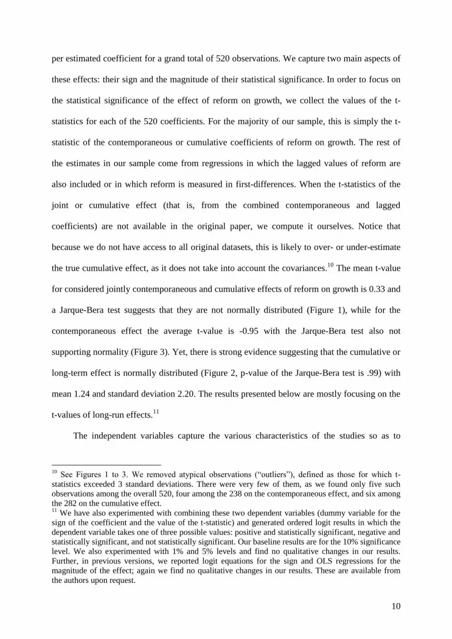
per estimated coefficient for a grand total of 520 observations. We capture two main aspects of

these effects: their sign and the magnitude of their statistical significance. In order to focus on

the statistical significance of the effect of reform on growth, we collect the values of the t-

statistics for each of the 520 coefficients. For the majority of our sample, this is simply the t-

statistic of the contemporaneous or cumulative coefficients of reform on growth. The rest of

the estimates in our sample come from regressions in which the lagged values of reform are

also included or in which reform is measured in first-differences. When the t-statistics of the

joint or cumulative effect (that is, from the combined contemporaneous and lagged

coefficients) are not available in the original paper, we compute it ourselves. Notice that

because we do not have access to all original datasets, this is likely to over- or under-estimate

the true cumulative effect, as it does not take into account the covariances.10

The mean t-value

for considered jointly contemporaneous and cumulative effects of reform on growth is 0.33 and

a Jarque-Bera test suggests that they are not normally distributed (Figure 1), while for the

contemporaneous effect the average t-value is -0.95 with the Jarque-Bera test also not

supporting normality (Figure 3). Yet, there is strong evidence suggesting that the cumulative or

long-term effect is normally distributed (Figure 2, p-value of the Jarque-Bera test is .99) with

mean 1.24 and standard deviation 2.20. The results presented below are mostly focusing on the

t-values of long-run effects.11

The independent variables capture the various characteristics of the studies so as to

10

See Figures 1 to 3. We removed atypical observations (“outliers”), defined as those for which t-

statistics exceeded 3 standard deviations. There were very few of them, as we found only five such

observations among the overall 520, four among the 238 on the contemporaneous effect, and six among

the 282 on the cumulative effect. 11

We have also experimented with combining these two dependent variables (dummy variable for the

sign of the coefficient and the value of the t-statistic) and generated ordered logit results in which the

dependent variable takes one of three possible values: positive and statistically significant, negative and

statistically significant, and not statistically significant. Our baseline results are for the 10% significance

level. We also experimented with 1% and 5% levels and find no qualitative changes in our results.

Further, in previous versions, we reported logit equations for the sign and OLS regressions for the

magnitude of the effect; again we find no qualitative changes in our results. These are available from

the authors upon request.

11

explain the large variation we observe in their findings. We focus on three main blocs of study

characteristics: method, measurement and specification. Under method, we are interested in,

inter alia, modelling features (number of observations, explanatory variables, and degrees of

freedom), choice of econometric technique and data characteristics (panel or cross-section and

the time period of the sample). Under measurement, we are basically interested in the way

reform is measured (which reforms, in levels versus changes, etc). And under specification, we

try to reflect the types and number of control variables (Appendix 2 has a complete list of these

variables).12

Let us comment on each of these blocs in turn.

In terms of general model features, for each of the 520 regressions reported in the 46

studies, we collect information on the number of observations, the number of explanatory

variables in each specification (including the reform variables) and on degrees of freedom. The

average number of explanatory variables from the regressions in our sample is about 10 and the

average degrees of freedom are slightly above 127 (with standard deviations of 8 and 80

respectively). The number of explanatory variables range from 2 to 58.

In terms of econometric modelling, we create dummy variables that: take the value of 1 if

the estimates are based on panel data (zero if cross-section), if fixed (country) effects are

present (zero otherwise), if fixed (time) effects are present (zero otherwise), and if reform is

treated as an endogenous variable (and zero otherwise). The choice of econometric modelling

reflects whether the possibility of endogeneity bias is addressed. This measure serves to answer

whether the assumption of exogeneity of reforms is supported, since significantly different

results from OLS and 2SLS or GMM would suggest the presence of two-way causation in the

growth-reform relationship. A vast majority of specifications (almost 80 percent) are estimated

on panel data, with just below a third of them addressing potential endogeneity bias and even

12

Notice that Appendix 2 has the full list of variables in our data set. For the sake of space, we do not

report results for all of them. We should mention that most MRA studies we know collect data on a

relatively smaller number of study characteristics and do not often use such a detailed and

comprehensive data set as ours (which contains 40 different potential explanatory variables.)

12

fewer making allowances for fixed effects.

As for the time windows used in the different studies, we create variables for the first

year of the sample, for the last year of the sample, and for its mid-point for each of the reported

regressions. Because output dynamics differ greatly across countries over time, we also create

dummy variables for all end years of the samples in each specification (which range from years

1993 to 2007). In case the author did not disclose the exact end year for each specification, we

assume all specifications (in each Table or paper) use the same one. The median starting and

ending years for our studies are 1990 and 1998, respectively. The variable coding the time

period covered in a particular study (early, middle, or late) is used to try to uncover changing

patterns of the significance of the effect over time.

Regarding different measures of reform and of reform dynamics, we construct a series of

dummy variables that take the value of 1 if the study used the EBRD overall average reform

index, the cumulative liberalization index (De Melo et al., 1997), simple averages of the World

Bank or EBRD indices, whether any of these individual reform components are used one at a

time, a combination of the EBRD and World Bank indices (and zero otherwise for each one of

these). Some authors use specific individual types of reform, thus we take advantage of the

correspondence between World Bank and EBRD indexes that the empirical literature uses to

code this possibilities as follows: a dummy variable was created taking the value of 1 if the

study uses the World Bank internal liberalization or the EBRD prices and labour markets

indexes; the World Bank external liberalization or EBRD trade and capital flows indexes; the

World Bank privatization or EBRD index small, large and banks privatization indexes; and

zero otherwise.13

In terms of measuring reform dynamics, we generate dummy variables that

13

There are large literatures assessing the effect of specific reforms. These are excluded from our study

because either they do not investigate more than one reform and/or they focus on individual countries.

One excellent case in point is the literature on privatization (reviews are provided by Megginson and

Netter, 2001, and, for the specific case of the transition economies, by Zinnes, Eilat, and Sachs, 2001,

and Hanousek, Kocenda, and Svejnar, 2007). See also Roland (2000) and Rozelle and Swinnen (2004)

13

take the value of 1 if both contemporaneous and lagged reforms are used, and if the reform

measure is a measure of its “speed,” or change over time. In addition, we capture whether the

estimation has a lagged dependent variable (1 if it does, zero otherwise) and whether quadratic

terms for reform are used (taking the value of 1 if they are, zero otherwise). We find that about

half of the specifications include both contemporaneous and lagged reforms and about a

quarter use speed as the preferred measure of reform.14

Next, regarding specification choice, we collect information on whether or not the

reported specifications includes variables for macroeconomic stabilization (as well as their

actual number), and in similar fashion for initial conditions, institutional development, and

factors of production (capital and labour). We also construct measures of whether or not the

results are reported separately for the former Soviet Union countries (split-sample analysis), for

whether or not initial conditions are proxied by the De Melo et al. (1997) principal components

indexes, for whether inflation is the stabilization measure used, for whether the study measures

underreported output,15

and for whether the study separates the effect of reform on public and

private sectors. Because approximately half of our coefficients come from authors whose main

affiliations are not academia (and for multiple authors, in all cases they share the same type of

affiliation), we also create a dummy variable for this characteristic.16

Finally, we also try to capture the quality of the paper, which is of course a very

for a discussion of the related theoretical literature. 14

Also note that all the studies in Appendix 1 focus on the so-called first generation reforms

(stabilization, liberalization, and privatization) but this is not because we do not believe that second

generation reforms (e.g., institutional and regulatory changes) are important; we simply do not know of

any econometric study that focuses on the latter type. 15

Official GDP figures for the years immediately following 1989 are widely believed to be biased

because statistical offices were not equipped to measure output from small private firms and because

prices were liberalised at different speeds. 16

This is quite common in MRA. For instance, Fidrmuc and Korhonen (2006) find that central bankers‟

estimates of business cycle correlation tend to be significantly more conservative (lower) than

academicians‟. Our prior in this case is that academicians‟ estimates will likely be lower than those

from non-academicians.

14

difficult task.17

We do so by constructing two variables. The first is a dummy variable

reflecting whether or not the paper is published in a peer-reviewed journal. Book chapters,

working papers and papers from conference proceedings are all coded zero in this dimension.

The second manner we devise to study paper quality is through the number of citations the

paper has received in Google Scholar (excluding self-citations). Google Scholar differs from

most other databases in that it includes published as well as unpublished papers. Citations are

calculated as average citations per year so as to try to adjust the impact of older papers.

4. Econometric Results

Despite the large econometric literature on the effects of economic reform on economic growth

during the transition from plan to market, the extent and depth of the divergence among results

is almost bewildering. As noted, any casual or informal attempt to take stock of the lessons

from this literature may be doomed from the start: a third of the large number of existing

estimates is positive and significant, another third is negative and significant, and the final third

is not statistically different from zero. In the case of the cumulative effect, the distribution

unsurprisingly shifts towards the positive side (Figure 3), but there is still huge variation. It is

our belief that MRA can be very useful in situations such as this one. In this section we present

and discuss our results using this technique.

We organise this presentation in terms of the three principal (potential) explanations we

offer for the existing divergence, namely we investigate whether differences in (a) methods, (b)

measurement, and (c) specification and quality of the empirical papers are the main reasons

that can potentially explain this variation. Our general-to-specific empirical strategy consists in

simultaneous testing of these three groups of factors. For sensitivity purposes, we also examine

17

Djankov and Murrell (2002) is the one paper we know that deals with the quality of the econometric

study, but it does so by constructing a subjective indicator. We are not aware of other meta-analysis

papers that measure quality objectively, like we do here.

15

the effects in each of these three groups of factors individually.

From the 46 studies listed Appendix 1, the values of the 276 normalised cumulative

effect t-test statistics range from –4.41 to 7.62 with mean 1.24 and standard deviation 2.20. The

aggregate test statistic is 62.20/1

M

k

k Mtt , which is statistically significant. The average

cumulative effect of reform on growth in transition economies is positive and significantly

different from zero. However, this descriptive statistic cannot represent such a diverse literature

given the variation in coefficients estimates we observe. Relying only on average test statistics,

we should refrain from inferring that there is strong robust relationship between growth and

reform. More importantly, this does not allow us to say much about the reasons for this rich

spectrum of estimates.

4.1 What explains the variance of the cumulative reform effect on growth?

4.1.a General-to-specific approach

The meta-regression model takes the form of equation (2) and the estimation strategy is based

on the general-to-specific principle. We start from a general specification encompassing all

explanatory variables, and then apply the backward stepwise method to selectively remove

variables.18

On each step, estimations are obtained by OLS with heteroskedasticity-consistent

standard errors.19

The final specification resulting from this procedure is shown in Table 1,

column 1. Overall, our final specification includes 10 significant characteristics, explaining

37% of variation in the data. These characteristics are as follows. Regarding estimation

method, we find degrees of freedom, the use of fixed effects and authors‟ affiliation to be

important factors. In terms of measurement, our results highlight the role of external

liberalization, whether multiple reforms are considered in the same specification and

18

All these results are confirmed if we use the forward stepwise regression approach instead. 19

We have also estimated all regressions reported in Tables 1 to 5 using the ordered probit model,

where the dependent variable takes the values of -1, 0, 1 if the coefficient of reform is negative and

significant at 10%, insignificant, and positive and significant at 10%, respectively. Results are

qualitatively the same as those reported here and are available upon request.

16

implementation speed. In terms of specification, we find that factors that help explain the

variance of the reform-growth effects are accounting for initial conditions, for institutions and

for macroeconomic stabilization. We also find that better papers, those with more average

yearly citations in Google Scholar, tend to report smaller effects of reform on growth. Let us

now discuss each of these main results in detail.

The results from method suggest that the higher the number of the degrees of freedom

in the original study or the larger the number of observations, the more likely it will be that the

study reports a positive and significant relationship between reform and growth. We also find

evidence that studies conducted by academicians (as opposed to author affiliated to think-

tanks, government institutes or international organizations) are less likely to support a positive

and significant reform–growth relationship. The -1.775 coefficient in Table 1, Column 1,

implies that, ceteris paribus, a paper written by academics would likely find a 1.775 lower

value of t-statistics. In other words, while the unconditional mean t-statistic for the cumulative

effect estimate is 1.777, a paper by academics would show, ceteris paribus, a near zero effect

(that is, a t-value of -0.002.) The use of country-specific dummies is also found to

systematically increase the probability of finding a positive reform-growth relationship.

Regarding the second block of the explanatory variables –reform measurement– the use

of external liberalization is associated with higher reform effect estimates. Yet if internal and

external liberalization and privatization are used one at time, our results show that the marginal

effect tends to be negative. Also when speed of the reform is used as explanatory variable, as

opposed to the reform level, the effect on growth is lower. This is indeed an important result

that reinforces the suggestion from this body of evidence that the growth payoffs from external

liberalization are larger than that from other structural reforms. Even accounting for other

important structural reforms, the effects of trade and capital liberalization seem to play a

significantly more pronounced role in driving up the existing reform on growth estimates. The

17

individual effect of including external liberalization is to increase the average t-value by 1.

From the third block, model specification and paper quality, we find that controlling for

initial conditions, institutions and stabilization decrease the estimated reform effect on growth.

Just to give an idea of the magnitude of these effects, a specification that includes initial

conditions variables will show a smaller average t-value, by about 0.6, all else the same. By the

same token, accounting for institutions lowers the mean t-statistics by about 0.4 points. Recall

that the average t-value for the long-run effect is 1.7 so these effects are indeed substantial.

Finally, we also find that more cited papers (measured by the number of citations the paper

receives according to Google Scholar per year) tend to report smaller effects of structural

reform on growth. Our results suggest that the effect of a paper receiving an additional 10

citations per year (in Google Scholar), calculated at the mean (which is 10.02 citations per

year), is to reduce the cumulative effect t-value by 0.38 (or by 0.29 for the results in Table 1,

column 2). Conditional on whether or not the paper has been published, the citation effect

changes: unpublished papers have an average of 5.38 citations per year and an increase of 10

more citations per year would reduce the average cumulative effect t-value by 0.57, while the

same effect for published papers (average 12.09 citations per year) would be reduce it by 0.33.

Since multiple estimates from the same study are used in our meta-regression

equations, we try to deal with the potential problem of biased sampling by including dummy

variables for each study. In the resulting specification, we find that 23 study dummies are

significant, indicating higher than conditional average probability to report a positive reform

effect in 13 and lower in 10 studies. More importantly, study dummies do not affect our key

main meta-regression results as none of the measurement, specification and study quality

characteristics loses significance (Table 1, column 2).20

From method, the degrees of freedom

20

It is important to stress that each of the cumulative and contemporaneous samples does not include

the entire set of 46 studies. In particular, the cumulative effect sample includes 40 out of the grand total

of 46 studies (hence, 39 study dummies are used in Table 1), while the contemporaneous effect sample

consists of 27 studies (thus 26 study dummies are used in Table 5). The correlation between study

18

and control for fixed effect estimates loose significance, yet authors‟ affiliation remains. We

thus conclude that the key determinants do not seem affected by biased sampling and that the

use of multiple estimates from the same study is valid in this case.

In the next three sub-sections we examine in more detail the variables from method-

measurement-specification and quality blocks. Although not all the variables appear in the final

specification, examination of their effects is useful to fully evaluate the sensitivity of the meta-

analysis results to the choice of control variables.

4.1.b The role of method

The results in Table 2 refer to the divergence of results in terms of various aspects of the choice

of econometric method in each study. A number of authors recognise the problem of the

potential endogeneity of reform vis-à-vis economic growth and address this by instrumental

variables, three-stage least squares, etc.21

Our meta-regression analysis reveals that those

studies that treat reform as endogenous are less likely to yield a positive and statistically

significant reform effect (Table 2, column 2). However, as shown below, this result is not

robust to the inclusion of other controls. The impact of reforms on growth is likely to follow a

J-curve over time as suggested by negative and statistically significant coefficient on the

variable capturing the sample mid-year (Table 2, column 4). In short, we find evidence that

three method variables help explain the variation in the estimated effects of reform on growth:

degrees of freedom, authors‟ affiliation and endogeneity correction.

4.1.c The role of measurement

The next set of factors we appraise is the way economic reform is measured. In this respect, we

distinguish the origin of the index (whether it was developed by the World Bank, EBRD, or a

combination of both) from the nature of the index (whether it internal or external liberalization,

dummies and authors‟ affiliation is generally low, with mean zero and range -.3 to .4. These results are

available upon request. 21

Among others, Heybey and Murrell, 1997; Kruger and Ciolko, 1997; Wolf, 1999; Berg et al., 1999;

Fidrmuc, 2001; Falcetti et al., 2002; Staehr, 2003; and Merlevede, 2003 – See Appendix 1.

19

privatization, their average, and their marginal effect if other reforms are also accounted for).

The results in Table 3 show that measuring reform by the EBRD index does not seem

to significantly affect the sign of the reform impact on growth performance. Yet, there is some

evidence that use of the World Bank‟s Cumulative Liberalization Index increases the

probability of finding a positive and significant effect of reform on growth, although this is not

robust to the inclusion of other controls. Among the three main types of reform considered in

the literature, the one highlighted in our results is external liberalization. Further, and maybe

not entirely surprising, if reform is measured by the average of its three main components

(internal and external liberalization and privatization), the effect is more likely to be positive

(Table 3, column 3). Surprisingly, however, internal liberalization and privatization measures

seem negatively associated with economic growth, albeit this effect is not robust. This set of

results supports the view that external liberalization plays a dominant role in driving up the

long-run effect of structural reforms (as a group) on economic growth.

The inclusion of lagged values of reform (Table 3, column 6) is one common way of

dealing with dynamics. We find that it increases the probability of the effect of reform on

growth to be negative and significant, and similarly with the use of speed as the measure of

reform. This finding in a sense supports the “no pain, no gain” view. The effect of structural

reforms seems to occur over a longer period of time, and reforms have large initial costs which

seem to be offset in subsequent years.

Column 8 in Table 3 shows our summary specification so far. Overall, six study

characteristics (namely, degrees of freedom, authors‟ affiliation, external liberalization,

average reform and speed) turn out to be important in explaining the variation in the

cumulative effect of reform on growth.

4.1.d The role of specification and quality of studies

The next set of variables reflects the choice of specification in the original study, in particular

20

the inclusion of specific sets of control variables. We pay special attention to (a) the inclusion

of controls for initial conditions, macroeconomic stabilization, institutional development and

factor inputs, (b) correcting for the possibility of underreported output, and (c) controlling for

the quality of a study by accounting for whether or not it is published in a refereed journal and

by the use of Google Scholar citations.

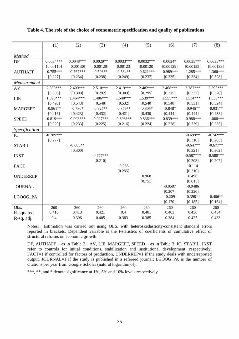
We find that controlling for initial conditions, macroeconomic stabilization, and

institutions significantly decreases the probability of finding a positive and significant impact

of reform and these remain after the inclusion of other control variables. Examining the value

of the coefficients on these variables from the last column of Table 4, we conclude that they

have a substantial impact. For instance, the presence of institutions in the underlying

econometric specification is associated with a decrease of the average t-value of the long-run

effect of reform on growth of approximately 0.742 (slightly larger than the effect discussed

above using the general to specific method, which is -0.624.)

Regarding study quality, we find that controlling for the study being published in a

refereed journal does not seem to systematically change the estimated reform effect (Table 4,

columns 5 and 6). On the other hand, accounting for the number of citations seems to deflate

the estimated reform effect (Table 4, columns 7 and 8).

In summary, ten study characteristics are deemed important in explaining the

significance of the cumulative reform effect (see Table 4, column 8), namely, the controls for

the degrees of freedom, author affiliation, average reform index, external liberalization,

multiple reforms, speed, controls for institutions, initial conditions, and stabilization, and

number of citations. We checked all our results for multicollinearity. The highest Variance

Inflation Factor (VIFs) we found was 3.48, which is considerably below the standard cut-off

value of 10, suggesting that multicollinearity is not a severe problem in this case.

21

4.2 What explains the variance of the contemporaneous reform effect on growth?

In order to asses the sensitivity of the results so far, we turn to the analysis of the

contemporaneous (or short-run) reform effect. Similar to the analysis above, of the

determinants of the cumulative or long-run reform effect on growth, the factors responsible for

the variance in the contemporaneous reform are assessed applying the general-to-specific

method (backward and forward stepwise regression). In addition, we also examine sequentially

the blocks of study characteristics, namely, method-measurement-specification and quality.

The main results from OLS estimations with heteroskedasticity-consistent standard errors are

reported in Table 5.

In the case of the contemporaneous effect, the regression sample has a smaller number

of observations (212) and fewer variables are present in the final specifications for the

(contemporaneous or short-term) effect of reform on growth. The determinants we find to be

important in this case are (with their impact on the probability of finding a positive and

significant reform effect in parentheses): controls for the later sample period (positive), fixed

effects (positive), external liberalization (positive), speed of reform (negative), lagged reform

(negative), institutions (negative), macroeconomic stabilization (negative), and publication in a

refereed journal (negative). One of the most interesting aspect of these results is that external

liberalization also seems to play a similar important, systematic and positive role in the short-

run, albeit now its effects seems dominated by that of macroeconomic stabilization.

Like the results presented for the cumulative effect, controlling for institutions and

stabilization is again associated with a lower probability of finding a positive and significant

impact of reforms on growth. Also, the use of lagged reform leads to a lower impact of

reforms, while the use of external liberalization increases the probability of a positive effect.

Similar to the case of the cumulative effect, the quality of publication matters; however it is

now that the study is published in a refereed journal (and not the number of citations) which

22

increases the probability of the contemporaneous effect to be negative. Column 1 in Table 5

presents our baseline model, where eight study characteristics are found to be significant,

explaining 51% of variation in test statistics.

An assessment of the concern about biased sampling was carried out by estimating the

above meta-regressions with study dummy variables (Table 5, column 2).22

We find that 13

study dummies are significant, indicating a higher than conditional average estimate of the

reform effect in eight studies and a systematically lower effect in five studies. Overall, for the

short-term or contemporaneous effect study fixed-effects seem to have a more substantial

impact on the meta-regression results (than in the long-run case). Indeed, out of eight

coefficients in the final specification, four lose their statistical significance. On this basis,

therefore, it is important to raise the possibility that biased sampling may be a more severe

issue in the short-run vis-à-vis the long-run case.

4.3 Discussion of additional sensitivity checks

The results above try to explain the variance of 260 coefficients on the long-run effect of

reforms on growth using the t-statistics of the cumulative reform effect as the dependent

variable. One first concern is that out these 260, 16 belong to regressions with several

alternative measures of reform used in the same equation. As noted, the results presented above

refer to the case in which those 16 most significant t-values were selected. One first sensitivity

check was to see whether our results change when the 16 least significant t-values are

employed instead. Overall, the results we obtain are very similar to those reported here.

We also experimented with the ordered dependent variable, taking the values of minus

one, zero and plus one to reflect the sign and significance of the reform effect. With respect to

the choice of the significance level, we investigate whether a 10%, 5% and 1% cut-off level

22

The VIF for these contemporaneous effect estimates with study dummies is 5.15, which is below the

cut-off value of 10.

23

would make a difference. Again, we experimented with the 16 most and least significant t-

values, and with contemporaneous versus cumulative reform effects. The results for the

cumulative reform effect and the contemporaneous reform effect are qualitatively similar to the

ones reported in this paper. 23

Finally, in earlier versions of the paper we experimented with an alternative coding of the

dependent variable, namely using separately the absolute values of the t-statistics and the sign

of the reform effect (either negative or positive, not distinguishing the insignificant estimates).

Also, we had different classification of short- and long-term effect estimates, allowing for

some overlap between the two set of estimates depending on the length of the time window the

study covered. The results are in line with the findings discussed above and are not reported for

the sake of space (these are also available upon request).

5. Conclusions

The objective of this paper is to take stock, summarise and evaluate the existing econometric

evidence on the effect of structural reforms on economic growth. This is carried out through

meta-regression analysis techniques using a unique data set covering more than 500 estimates

of the effect of reform on growth from more than 40 econometric studies. Overall, the direction

of the effect of structural reforms on economic performance and its statistical significance

depends on whether the contemporaneous or the cumulative impact is considered. In the short-

term, reforms have a non-negligible cost and no immediate impact on growth. The positive

effects of structural reforms on growth materialize with some time lag. We present evidence

that the average magnitude of the long-run reform effect on growth is substantially larger than

that of the average short-term effect. Moreover, the impact of reforms on growth is sensitive to

the specification, modelling choice, as well as various co-determinants such as institutions and

23

These results are available upon request from the authors.

24

initial conditions. The use of lagged reform measures shows that reforms have negative

contemporaneous (short-run) effects which are offset by positive effects in subsequent periods

(long-term). We also find that the existing results seem to be sensitive to the choice of the

measure of reform used.

The results of our meta-regression analysis illustrate that ignoring the estimation

method (in particular the use of country-specific effects) is dangerous. Our findings suggest

that accounting for country-specific effects (for both cumulative and contemporaneous effects)

and the time coverage (for the contemporaneous effect) are important in explaining the

variation in the estimated effects. Further, the one aspect of reform packages that seems to

receive overwhelming support in our data is the liberalization of trade and capital flows (that is,

external liberalization). The loss of statistical significance from liberalization in the case of

contemporaneous effect is counterbalanced by the importance of macroeconomic liberalization,

in the short-run. Of particular interest is the finding that controlling for institutions and initial

conditions appears to be very effective in decreasing the probability of finding a large and

positive effect of reform on growth, both in the short- and in the long-run.

These findings are useful in suggesting directions for future research. We highlight

four. (1) Considerably more attention should be paid to measurement issues. There are well-

known measurement problems with respect to economic reforms. As for GDP growth, the early

official data seems to underestimate the participation of the nascent private sector (in some

cases because of the large informal sectors) and overestimate that of the public sector. With

respect to reform, the existing measures are mostly subjective, difficult to replicate and tend

not to capture reform reversals. In more concrete terms, it is somewhat surprising that we were

not able to find one study that pays attention to the problem of errors-in-variables. Therefore,

studies that try to deal with this matter in the future will likely make important contributions.

(2) Our findings suggest that the use of measures of external liberalization is central in

25

understanding growth performance, yet almost no study we examine attempts to investigate

how this reform interacts with other reforms such as privatization or labour market

liberalization. Recall that the backdrop is a theoretical literature in which the issue of the

sequencing of reforms looms large and a policy debate in which the big-bang versus

gradualism options are discussed, as this paper demonstrates, without much robust underlying

econometric evidence. Therefore more attention to the issue of reform sequencing and

interactions among reforms should also generate genuine contributions in future work. (3) The

difference in the average values of t-statistics between the short-run and the long-run

(contemporaneous and cumulative) indicates that our data captures well the trade-off that many

thought was at the essence of debates on reform strategy, namely the welfare effect of an

immediate large decline followed by a long rise. Future research, using better data and longer

time windows, would do well in trying to jointly estimate the short- and long-run effects24

and

use these results to calculate the discount rates that make the overall effects of reform zero

given the short-term loss and the long-term gain. (4) Efforts could also be made in terms of

making explicit the theoretical framework guiding the econometric analysis. In very few of the

studies reviewed above can one identify concerns in this respect. In particular, a better

understanding of the reasons why the long-run impact of reforms on growth tends to be

positive while in the short-run it seems to have non-negligible costs, and particularly the role

institutions play in this asymmetry, would be welcome. Because we now have more than 15

years of data available, it is perhaps high time to improve upon this aspect.

24

See Loayza and Rancière (2006) for an example of the joint estimation of the short- and long-run

effects, in their case, of financial liberalization on economic growth.

26

References

Acemoglu, Daron, Johnson, Simon, Robinson, James, 2005. Institutions as the Fundamental

Cause of Long-Run Growth. In: Aghion, Philippe, Durlauf, Stephen (Eds.), Handbook of

Economic Growth, Vol. 1, Ch. 6. Elsevier, pp. 385–472.

Ashenfelter, Orley, Harmon, Colm P., Oosterbeek, Hessel, 1999. A Review of Estimates of

the Schooling/Earnings Relationship, with Tests for Publication Bias. Labour Economics 6

(4), 453–470.

Campos, Nauro F., Coricelli, Fabrizio, 2002. Growth in Transition: What We Know, What

We Don‟t, and What We Should. Journal of Economic Literature 40 (3), 793–836.

Card, David and Krueger, Alan B., 1995. Time-Series Minimum Wage Studies: a Meta-

Analysis. The American Economic Review 85 (2), 238–243.

Djankov, Simeon, Murrell, Peter, 2002. Enterprise Restructuring in Transition: A Quantitative

Survey. Journal of Economic Literature 40 (3), 736–792.

De Melo, Martha, Denizer, Cevdet, Gelb, Alan, 1997. From Plan to Market: Patterns of

Transition. In: Blejer, Mario I., Skreb, Marko (Eds.), Macroeconomic Stabilization in

Transition Economies. Cambridge University Press, Cambridge, pp. 17–72.

Doucouliagos, Chris, 1995. Worker Participation and Productivity in Labor-Managed and

Participatory Capitalist Firms: A Meta-Analysis. Industrial and Labor Relations Review 49

(1), 58–77.

Durlauf, Steven N., Johnson, Paul A., Temple, Jonathan, R. W., 2005. Growth Econometrics.

In Aghion, Philippe, Durlauf, Stephen (Eds.), Handbook of Economic Growth, Vol. 1, Ch. 8.

Elsevier, pp. 555–677.

Égert, Balazs, Halpern, László, 2006. Equilibrium Exchange Rates in Central and Eastern

Europe: A Meta-Regression Analysis. Journal of Banking and Finance 30 (5), 1359–1374.

Fidrmuc, Jarko, Korhonen, Iikka, 2006. Meta-Analysis of the Business Cycle between the

Euro Area and the CEECs. Journal of Comparative Economics 34 (3), 518–537.

Fischer, Ronald A., 1932. Statistical Methods for Research Workers. 4th edition, Oliver and

Boyd, London.

Florax, Raymond J. G. M., 2002. Meta-Analysis in Environmental and Natural Resource

Economics: The Need for Strategy, Tools and Protocol. Department of Spatial Economics,

Free University, Amsterdam.

Florax, Raymond J. G. M., de Groot, Henri L. F., De Mooij, Ruud A., 2002. Meta-Analysis: A

Tool for Upgrading Inputs of Macroeconomic Policy Models. Discussion Paper No. TI 041/3.

Tinbergen Institute, Amsterdam.

Glass, Gene V., 1976. Primary, Secondary, and Meta-Analysis of Research. The Educational

Researcher, 5 (10), 3–8.

27

Hanousek, Jan, Kocenda, Evzen, Svejnar, Jan, 2007. Origin and Concentration: Corporate

Ownership, Control and Performance in Firms after Privatization. The Economics of

Transition 15 (1), 1–31.

Havrylyshyn, Oleh, 2001. Recovery and Growth in Transition: A Decade of Evidence. IMF

Staff Papers, 48 (4), 53–87.

Hedges, Larry V., Olkin, Ingram, 1985. Statistical Methods for Meta-Analysis. Academic

Press, Orlando.

Jarrell, Stephen B., Stanley, Tom D., 1990. A Meta-Analysis of the Union-Non-Union Wage

Gap. Industrial and Labor Relations Review, 44 (1), 54–67.

Levine, Ross, Renelt, David, 1992. A Sensitivity Analysis of Cross-Country Growth

Regressions. The American Economic Review 82 (4), 942–963.

Light, Richard J. and Smith, Paul V., 1997. Accumulating Evidence: Procedures for Resolving

Contradictions Among Different Research Studies. Harvard Educational Review 41 (4), 429–

471.

Loayza, Norman V., Rancière, Romain, 2006. Financial Development, Financial Fragility and

Growth. Journal of Money Credit and Banking 38 (4), 1051-1076.

Megginson, William L., Netter, Jeffry M, 2001. From State to Market: A Survey of Empirical

Studies on Privatization. Journal of Economic Literature, 39(2), 321–389.

Phillips, Josef M., Goss, Ernest P., 1995. The Effect of State and Local Taxes on Economic

Development: A Meta-Analysis. Southern Economic Journal 62 (2), 320–333.

Roland, Gérard, 2000. Transition and Economics: Politics, Markets and Firms. MIT Press,

Cambridge, MA.

Rose, Andrew K., Stanley, Tom D. 2005. A Meta-Analysis of the Effect of Common

Currencies on International Trade. Journal of Economic Surveys 19 (3), 347–365.

Rozelle, Scott, Swinnen, Johan F. M., 2004. Success and Failure of Reforms: Insights from

Transition Agriculture. Journal of Economic Literature 42 (2), 404 – 456.

Stanley, Tom D., 1998. New Wine in Old Bottles: A Meta-Analysis of Ricardian Equivalence.

Southern Economic Journal 64 (3), 713–727.

Stanley Tom D., 2001. Wheat From Chaff: Meta-Analysis as Quantitative Literature Review.

Journal of Economic Perspectives 15 (3), 131–150.

Stanley, Tom D., 2005. Beyond Publication Bias. Journal of Economic Surveys 19 (3), 309–

345.

Stanley Tom D., Jarrell, Stephen B., 1998. Gender Wage Discrimination Bias? A Meta-

Regression Analysis. Journal of Human Resources 33 (4), 947–973.

28

Stanley, Tom D., Jarrell, Stephen B., 1989. Meta-Regression Analysis: A Quantitative Method

of Literature Surveys. Journal of Economic Surveys 19 (3), 54–67.

Weichselbaumer, Doris, Winter-Ebmer, Rudolf, 2007. The Effects of Competition and Equal

Treatment Laws on the Gender Wage Differentials. Economic Policy, 22 (50), 235–287.

Zinnes, Clifford, Eilat, Yair, Sachs, Jeffrey, 2001. The Gains from Privatization in Transition

Economies: Is „Change of Ownership‟ Enough? IMF Staff Papers, 48 (4), 146–170.

29

Figure 1.

Histogram of the t-statistics of coefficients of structural reforms on economic growth

515 coefficients from the 46 papers listed in Appendix 1 (Excludes 5 outliers: coefficients

whose t-statistics exceed 3 standard deviations)

0

.05

.1.1

5

Den

sity

-10 -5 0 5 10lib_all

30

Figure 2.

Histogram of the t-statistics of coefficients of contemporaneous structural reforms on

economic growth: 234 coefficients from papers listed in Appendix 1 (Excludes 4 outliers:

coefficients whose t-statistics exceed 3 standard deviations)

0

.05

.1.1

5.2

Den

sity

-10 -5 0 5 10lib

31

Figure 3.

Histogram of the t-statistics of coefficients of cumulative effect of structural reforms on

economic growth: 276 coefficients from papers listed in Appendix 1 (Excludes 6 outliers:

coefficients whose t-statistics exceed 3 standard deviations)

0

.05

.1.1

5.2

.25

Den

sity

-5 0 5 10lib_cum

32

Table 1. The determinants of the cumulative reform effect: General-to-specific results

(1)a (2)

b

Method

DF 0.00262* 0.00047

[0.00151] [0.00146]

AUTHAFF -1.775*** -4.024***

[0.399] [0.359]

FIXED 1.105*** -0.434

[0.388] [0.415]

Measurement

LIE 1.009* 1.449***

[0.585] [0.534]

MARGEFF -2.793*** -1.683***

[0.450] [0.476]

SPEED -2.056*** -1.946***

[0.240] [0.328]

Specification & Quality

IC -0.624** -1.139***

[0.303] [0.390]

INST -0.431* -0.952***

[0.234] [0.337]

STABIL -0.987*** -0.672**

[0.306] [0.319]

LGOOG_PA -0.541*** -0.414*

[0.182] [0.224]

Observations 260 260

R-squared 0.367 0.649

R-squared adjusted 0.341 0.598

Notes:

a These results are obtained using the general-to-specific method, backwards stepwise regression, which

is confirmed by the forward stepwise results. It reports the final specification from using all the Method-

measurement-specification and quality variables at once and as a starting point.

b Estimated with 39 study dummies (not shown). 23 dummies are significant, out of which 13 are

positive and 10 are negative.

Estimation was carried out using OLS, with heteroskedasticity-consistent standard errors reported in

brackets. Dependent variable is the t-statistics of coefficients of cumulative effect of structural reforms

on economic growth.

DF is degrees of freedom, AUTHAFF is author‟s affiliation (1 if non-academic, zero otherwise),

FIXED is a dummy variable that takes the value of 1 if country-specific dummy variables are included,

LIE, LII and LIP refer to external liberalization; internal and/or price liberalization, and privatization

and banking reform, respectively; MARGEFF=1 if LII, LIE, LIP are used jointly; SPEED=1 if speed is

the measure of reform. IC, STABIL, INST refer to controls for initial conditions, stabilization and

institutional development, respectively; LGOOG_PA is the number of citations per year from Google

Scholar (natural logarithm of).

***, **, and * denote significance at 1%, 5% and 10% levels respectively.

33

Table 2. The determinants of the reform-growth effect: The role of method

(1) (2) (3) (4) (5)

Method DF 0.00365** 0.00400* 0.00360* 0.00427 0.00355**

[0.00144] [0.00224] [0.00188] [0.00269] [0.00159]

AUTHAFF -0.781*** -0.761** -0.767***

[0.276] [0.295] [0.269]

PANEL -0.142 -0.113

[0.403] [0.429]

FIXED 0.01 -0.0832

[0.433] [0.460]

ENDO -0.843** -0.864** -0.833***

[0.333] [0.336] [0.317]

EARLY 0.497 0.169

[0.338] [0.332]

MIDDLE -0.46 -0.496*

[0.284] [0.285]

LATE 0.323 0.32

[0.369] [0.366]

Observations 260 260 260 260 260

R-squared 0.0263 0.0985 0.0466 0.113 0.0981

R-squared adj 0.0226 0.0808 0.0316 0.0843 0.0875

Notes:

Estimation was carried out using OLS, with heteroskedasticity-consistent standard errors reported in

brackets. Dependent variable is the t-statistics of coefficients of cumulative effect of structural reforms

on economic growth.

DF is degrees of freedom, AUTHAFF is author‟s affiliation (1 if non-academic, zero otherwise),

PANEL is a dummy variable that takes the value of 1 if the reform-growth coefficient is from panel

data, FIXED is a dummy variable that takes the value of 1 if country-specific dummy variables are

included, ENDO is 1 if there is an attempt to deal with endogeneity bias (zero otherwise), MIDDLE,

EARLY and LATE refer to the time windows used for estimation (1989-1993, 1994-1998 and 1999-

2007, respectively).

***, **, and * denote significance at 1%, 5% and 10% levels respectively.

34

Table 3. The role of the measurement of reform and reform dynamics

(1) (2) (3) (4) (5) (6) (7) (8)

Method

DF 0.0045*** 0.0038** 0.0030** 0.0035*** 0.0034** 0.0071*** 0.0061*** 0.0031**

[0.00164] [0.00173] [0.00133] [0.00132] [0.00134

]

[0.00144] [0.00145] [0.00120]

AUTHAFF -0.889*** -0.704** -0.671*** -0.401* -0.425* -0.861*** -0.575* -0.661***

[0.267] [0.314] [0.236] [0.239] [0.257] [0.236] [0.298] [0.234]

ENDO -0.770** -0.824*** -0.137 -0.098 -0.107 -0.822*** -0.323

[0.319] [0.317] [0.302] [0.294] [0.294] [0.287] [0.291]

Measurement

CLI 1.226*** -0.256

[0.402] [0.494]

EBRD -0.127 -0.316

[0.293] [0.311]

AV 2.679*** 2.441*** 2.491***

[0.265] [0.781] [0.293]

LIE -1.538*** -1.382** 1.842* 1.533***

[0.537] [0.599] [0.998] [0.538]

LII -3.082*** -

3.011***

0.203

[0.427] [0.497] [0.960]

LIP -3.283*** -

3.220***

0.353

[0.291] [0.305] [0.904]

MARGEFF -0.208 -0.722 -0.826*

[0.474] [0.442] [0.428]

SPEED -1.034*** -0.522** -0.829***

[0.273] [0.253] [0.220]

LAGS -1.574*** -1.189***

[0.271] [0.289]

Obs. 260 260 260 260 260 260 260 260

R-squared 0.124 0.0987 0.356 0.374 0.375 0.299 0.445 0.398

R-sq. adj. 0.11 0.0846 0.346 0.359 0.357 0.285 0.418 0.384

Notes: Estimation was carried out using OLS, with heteroskedasticity-consistent standard errors

reported in brackets. Dependent variable is the t-statistics of coefficients of cumulative effect of

structural reforms on economic growth.

DF, AUTHAFF, ENDO – as in Table 2. CLI=1 if the cumulative liberalization index from the World

Bank is used as a reform measure, EBRD=1 if the reform index originates from the EBRD, AV=1 if

average (simple or weighted, or simple sum) of reform indices LIE, LII or LIP was used; LIE, LII and

LIP refer to external liberalization; internal and/or price liberalization, and privatization and banking

reform, respectively; MARGEFF=1 if LII, LIE, LIP are used jointly; SPEED=1 if speed is the measure

of reform, LAGS=1 if both contemporaneous and lagged reform variables are used.

***, **, and * denote significance at 1%, 5% and 10% levels respectively.

35

Table 4. The role of the choice of econometric specification and quality of publications

Notes: Estimation was carried out using OLS, with heteroskedasticity-consistent standard errors

reported in brackets. Dependent variable is the t-statistics of coefficients of cumulative effect of

structural reforms on economic growth.

DF, AUTHAFF – as in Table 2. AV, LIE, MARGEFF, SPEED – as in Table 3. IC, STABIL, INST

refer to controls for initial conditions, stabilization and institutional development, respectively;

FACT=1 if controlled for factors of production, UNDERREP=1 if the study deals with underreported

output, JOURNAL=1 if the study is published in a refereed journal; LGOOG_PA is the number of

citations per year from Google Scholar (natural logarithm of).

***, **, and * denote significance at 1%, 5% and 10% levels respectively.

(1) (2) (3) (4) (5) (6) (7) (8)

Method DF 0.0034*** 0.0048*** 0.0029** 0.0033*** 0.0032*** 0.0024* 0.0035*** 0.0035***

[0.00110] [0.00130] [0.00120] [0.00123] [0.00120] [0.00129] [0.00135] [0.00133]

AUTHAFF -0.755*** -0.767*** -0.503** -0.584** -0.621*** -0.989*** -1.285*** -1.360***

[0.227] [0.234] [0.238] [0.249] [0.237] [0.335] [0.334] [0.328]

Measurement

AV 2.569*** 2.409*** 2.510*** 2.419*** 2.482*** 2.468*** 2.387*** 2.395***

[0.306] [0.300] [0.292] [0.303] [0.295] [0.315] [0.337] [0.320]

LIE 1.590*** 1.464*** 1.486*** 1.540*** 1.539*** 1.555*** 1.534*** 1.535***

[0.496] [0.543] [0.548] [0.532] [0.540] [0.548] [0.531] [0.524]

MARGEFF -0.861** -0.780* -0.927** -0.876** -0.805* -0.848* -0.945** -0.931**

[0.416] [0.423] [0.432] [0.421] [0.430] [0.444] [0.444] [0.438]

SPEED -0.819*** -0.903*** -0.927*** -0.808*** -0.836*** -0.839*** -0.988*** -1.008***

[0.220] [0.233] [0.225] [0.216] [0.224] [0.228] [0.239] [0.235]

Specification

IC -0.789*** -0.699** -0.742***

[0.277] [0.310] [0.283]

STABIL -0.685** -0.647** -0.677**

[0.300] [0.321] [0.302]

INST -0.777*** -0.587*** -0.580***

[0.210] [0.208] [0.207]

FACT -0.238 -0.114

[0.255] [0.310]

UNDERREP 0.968 0.496

[0.751] [0.615]

JOURNAL -0.0507 -0.0486

[0.207] [0.226]

LGOOG_PA -0.209 -0.398** -0.406**

[0.170] [0.185] [0.164]

Obs. 260 260 260 260 260 260 260 260

R-squared 0.416 0.413 0.421 0.4 0.401 0.403 0.456 0.454

R-sq. adj. 0.4 0.396 0.405 0.383 0.385 0.384 0.427 0.433

36

Table 5. The determinants of the contemporaneous reform effect: General-to-specific

approach

(1)a (2)

b

Method

LATE 1.756*** 0.804*

[0.436] [0.466]

FIXED 1.479*** 0.341

[0.513] [0.379]

Measurement

LIE 2.024*** 0.521

[0.725] [0.674]

SPEED -1.313*** -0.893**

[0.502] [0.367]

LAGS -3.934*** -2.944***

[0.527] [0.406]

Specification & Quality

INST -2.057*** 0.124

[0.522] [0.224]

STABIL -2.354*** -1.257**

[0.671] [0.621]

JOURNAL -1.243*** -0.103

[0.432] [0.370]

Observations 212 212

R-squared 0.505 0.795

R-squared adjusted 0.485 0.772

Notes:

a These results are obtained using the general-to-specific method, backwards stepwise regression, which

is confirmed by the forward stepwise results. It reports the final specification from using all the Method-

measurement-specification and quality variables at once and as a starting point.

b Estimated with 26 study dummies (not shown). 13 dummies are significant, out of which 8 are positive

and 5 are negative.

Estimation was carried out using OLS, with heteroskedasticity-consistent standard errors reported in

brackets. Dependent variable is the t-statistics of coefficients of contemporaneous effect of structural

reforms on economic growth.

LATE is the time windows used for estimation (1999-2007), FIXED is a dummy variable that takes the

value of 1 if country-specific dummy variables are included, CLI=1 if the cumulative liberalization

index from the World Bank is used as a reform measure, LIE=1 if external liberalization component

were used as a reform measure, SPEED=1 if speed is the measure of reform, LAGS=1 if both

contemporaneous and lagged reform variables are used, INST=1 if controlled for institutional

development, STABIL=1 if controlled for stabilization, JOURNAL=1 if the study is published in a

refereed journal.

***, **, and * denote significance at 1%, 5% and 10% levels respectively.

37

APPENDIX 1.

Econometric studies of the effect of structural reforms on economic growth

(1) Abed, George T. and Hamid R. Davoodi, 2002. “Corruption, Structural Reforms, and

Economic Performance in the Transition Economies,” in Abed, George T. and Sanjeev

Gupta (eds.), Governance, corruption, and economic performance, pp. 489–537.

Washington, D.C.: International Monetary Fund.

(2) Ahrens, Joachim and Martin Meurers, 2002. “How Governance Affects the Quality of

Policy Reform and Economic Performance: New Evidence for Economies in Transition,”

Journal of Institutional Innovation, Development and Transition, 6, pp. 35–56.

(3) Åslund, Anders, Peter Boone and Simon Johnson, 1996. “How to Stabilize: Lessons from

Post-Communist Countries,” Brookings Papers on Economic Activity 1, pp. 217–91.

(4) Aziz, Jahangir and Robert F. Wescott, 1997. “Policy Complementarities and the

Washington Consensus,” IMF WP, No. 97/118.

(5) Beck, Thorsten and Luc Laeven, 2006. “Institution Building and Growth in Transition

Economies,” Journal of Economic Growth, 11(2), pp. 157–86.

(6) Berg, Andrew, Eduardo Borensztein, Ratna Sahay and Jeromin Zettelmeyer, 1999. “The

Evolution of Output in Transition Economies: Explaining the Differences,” IMF WP, No.

99/73.

(7) Braga de Macedo, Jorge and Joaquim Oliveira Martins, 2008. “Growth, Reform Indicators

and Policy Complementarities,” Economics of Transition, 16(2), pp. 141–64.

(8) Christoffersen, Peter and Peter Doyle, 2000. “From Inflation to Growth: Eight Years of

Transition,” Economics of Transition, 8(2), pp. 421–51.

(9) Cungu, Azeta and Johan Swinnen, 2003. “The Impact of Aid on Economic Growth in

Transition Economies: An Empirical Study,” LICOS Discussion Paper, No. 128/2003.

(10) De Melo, Martha, Cevdet Denizer and Alan Gelb, 1997. “From Plan to Market:

Patterns of Transition,” in: Blejer, Mario I. and Škreb, Marko (eds.), Macroeconomic

Stabilization in Transition Economies, pp. 17–72. Cambridge: Cambridge University Press.

(11) De Melo, Martha, Cevdet Denizer, Alan Gelb and Stoyan Tenev, 2001. “Circumstance

and Choice: The Role of Initial Conditions and Policies in Transition Economies,” World

Bank Economic Review, 15(1), pp. 1–31.

(12) Denizer, Cevdet, 1997. “Stabilization, Adjustment, and Growth Prospects in Transition

Economies,” World Bank Policy Research Working Paper, No. 1855.

(13) Eschenbach, Felix and Bernard Hoekman, 2006. “Services Policy Reform and Economic

Growth in Transition Economies,” Review of World Economics, 142(4), pp. 746–64.

38

(14) Falcetti, Elisabetta, Tatiana Lysenko and Peter Sanfey, 2006. “Reforms and Growth in

Transition: Re-examining the Evidence,” Journal of Comparative Economics, 34(3), pp.

421–45.

(15) Falcetti, Elisabetta, Martin Raiser, and Peter Sanfey, 2002. “Defying the Odds: Initial

Conditions, Reforms, and Growth in the First Decade of Transition,” Journal of

Comparative Economics, 30(2), pp. 229–50.

(16) Fidrmuc, Jan, 2003. “Economic Reform, Democracy and Growth during Post-communist

Transition,” European Journal of Political Economy, 19 (3), pp. 583–604.

(17) Fidrmuc, Jan, 2001. “Forecasting Growth in Transition Economies: A Reassessment,”

Bonn, Center for European Integration Studies, mimeo.

(18) Fidrmuc, Jan and Ariane Tichit, 2004. “Mind the Break! Accounting for Structural

Breaks in Growth during Transition,” William Davidson Institute Working Paper, No. 643.

(19) Fidrmuc, Jan and Ariane Tichit, 2009. “Mind the Break! Accounting for Structural

Breaks in Growth during Transition,” Economic Systems, 33(2), pp. 138–54. [Results in the

published version (19) are different from (18) in terms of methods and robustness]

(20) Fischer, Stanley and Ratna Sahay, 2004. "Transition Economies: The Role of Institutions

and Initial Conditions," IMF Conference in Honour of Guillermo Calvo.

(21) Fischer, Stanley and Ratna Sahay, 2001. “The Transition Economies After Ten Years,”

in: Orlowski, Lucjan T. (ed.) Transition and Growth in Post-communist Countries: The

Ten-year Experience, pp. 3–47. Cheltenham, UK and Northampton, MA, USA: Edward

Elgar.

(22) Fischer, Stanley, Ratna Sahay and Carlos A. Végh, 1998. “From Transition to Market:

Evidence and Growth Prospects,” IMF Working Paper, No. 98/52.

(23) Fischer, Stanley, Ratna Sahay and Carlos Végh, 1996a. “Economies in Transition: The

Beginnings of Growth,” American Economic Review, 86(2), pp. 229–33.

(24) Fischer, Stanley, Ratna Sahay and Carlos Végh, 1996b. “Stabilization and Growth in

Transition Economies: The Early Experience,” Journal of Economic Perspectives 10(2),

pp. 45–66.

(25) Godoy, Sergio and Joseph E. Stiglitz, 2006. “Growth, Initial Conditions, Law and Speed

of Privatization in Transition Countries: 11 Years Later,” NBER Working Paper, No.

11992.

(26) Havrylyshyn, Oleh and Ron van Rooden, 2003. “Institutions Matter in Transition, But So

Do Policies,” Comparative Economic Studies, 45(1), pp. 2–24.

(27) Havrylyshyn, Oleh, Ivailo Izvorski and Ron van Rooden, 2001. “Recovery and Growth

in Transition Economies 1990–97: A Stylised Regression Analysis,” in: Hoen, Herman W.

(ed.) Good governance in Central and Eastern Europe: The Puzzle of Capitalism by

Design, pp. 26–53. Economies and Societies in Transition series. Cheltenham, UK and

Northampton, MA, USA: Edward Elgar.

39

(28) Hernandez-Cata, Ernesto, 1997. “Liberalization and the Behavior of Output During the

Transition from Plan to Market,” IMF Staff Papers, No. 44(4), pp. 405–29.

(29) Heybey, Berta and Peter Murrell, 1999. “The Relationship between Economic Growth

and the Speed of Liberalization,” Journal of Policy Reform, 3(2), pp. 121–37.

(30) Kim, Byung-Yeon and Jukka Pirttila, 2003. “The Political Economy of Reforms:

Empirical Evidence from Post-Communist Transition in the 1990s,” Bank of Finland,

Institute for Economies in Transition Discussion Paper, No. 4.

(31) Krueger, Gary and Marek Ciolko, 1998. “A Note on Initial Conditions and Liberalization

during Transition,” Journal of Comparative Economics, 26(4), pp. 718–34.

(32) Lawson, Colin and Haifeng Wang, 2005. “Economic Transition in Central and Eastern

Europe and the Former Soviet Union: Which Policies Worked?” University of Bath,

Department of Economics and International Development, Working Paper, No. 01-05.

(33) Loungani, Parkash and Nathan Sheets, 1997. “Central Bank Independence, Inflation and

Growth in Transition Economies,” Journal of Money, Credit and Banking, 29(3), pp. 381–

99.

(34) Merlevede, Bruno, 2003. “Reform Reversals and Output Growth in Transition

Economies,” Economics of Transition, 11(4), pp. 597–751.

(35) Mickiewicz, Tomasz M., 2005. “Post-Communist Recessions Re-examined,” in:

Mickiewicz, Tomasz M., Economic Transition in Central Europe and the Commonwealth

of Independent States, Ch.6, pp.99–118. Houndsmill: Palgrave Macmillan.

(36) Mickiewicz, Tomasz M., 2005. “Is The Link Between Reforms and Growth Spurious? A

Comment,” in: Mickiewicz, Tomasz M., Economic Transition in Central Europe and the

Commonwealth of Independent States, Ch.10, pp.181–96. Houndsmil: Palgrave Macmillan.

(37) Neyapti, Bilin and Nergiz Dincer, 2005. “Measuring Quality of Bank Regulation and

Supervision, with an Application to Transition Economies,” Economic Inquiry, 43, pp. 79–

99.

(38) Pelipas, Igor and Chubrik, Alexander, 2008, “Market Reforms and Growth in Post-

socialist Economies: Evidence from Panel Cointegration and Equilibrium Correction

Model,” WDI Working Paper, No. 936.

(39) Piculescu, Violeta, 2003, “Direct and Feedback Effects on Economic and Institutional

Developments in Transition: A Path Analysis Approach,” Goteborg University, mimeo.

(40) Polanec, Sašo, 2004, “Convergence at Last? Evidence from Transition Countries,”

Eastern European Economics, 42(4), pp. 55–80.

(41) Radulescu, Roxana and David Barlow, 2002. “The Relationship between Policies and

Growth in Transition Countries,” Economics of Transition, 10(3), pp. 719–45.

40

(42) Radziwill, Artur and Pawel Smietanka, 2009. “EU's Eastern Neighbours: Institutional

Harmonisation and Potential Growth Bonus,” CASE Network Studies and Analyses, No.

386.

(43) Sachs, Jeffrey D., 1996. “The Transition at Mid-Decade,” American Economic Review,

Papers and Proceedings, 86 (2), pp. 128–33.

(44) Selowsky, Marcelo and Ricardo Martin, 1997. “Policy Performance and Output Growth

in the Transition Economies,” American Economic Review 87(2), pp. 349–53.

(45) Staehr, Karsten, 2005. “Reforms and Economic Growth in Transition Economies:

Complementarity, Sequencing and Speed,” European Journal of Comparative Economics,

2(2), pp. 177–202.

(46) Wolf, Holger C., 1999. “Transition Strategies: Choices and Outcomes,” Princeton

Studies in International Finance, 85 (June), pp. 1–30.

41

APPENDIX 2.

Description of variables in MRA data set

Dependent variables:

REF: t-statistic of coefficients of either cumulative or contemporaneous effect of structural

reforms on economic growth.

REF_3_10 = -1, 0, and 1 if the coefficient on either cumulative or contemporaneous reform is

negative and significant at 10%, insignificant, and positive and significant at 10%,

respectively.

Meta-independent variables:

I) Method

N = the number of observations in the individual study

K = the number of explanatory variables

DF = N–K is the degrees of freedom reflecting power of the test statistics

AUTHAFF = 1 if all authors are from academia, =0 if at least one of the authors is not

Econometric technique

PANEL = 1 if the model uses panel data, =0 if cross-section

ENDO =1 if model used is 2SLS, 3SLS, GMM, cointegration; =0, otherwise

FIXED = 1 if fixed effects estimation is used (or country dummies)

Time period

START = first year of the sample

END = end year of the sample

MID = (START+END)/2 is the average year of the sample

EARLY =1 if the sample is 1989-1993

MIDDLE =1 if the sample is 1994-1998

LATE = 1 if the sample is 1999-2007

E93 – E07 = dummy for the end year of the data sample (1993 – 2007 respectively)

II) Measurement

a) Origin of the index. Each index belongs to one of the following four types:

WB = 1 if the reform index originates from the World Bank only

EBRD = 1 if the reform index originates from the EBRD only

COMB = 1 if a combination of EBRD and WB indices is used

OTHER = 1 if the share of private sector in GDP or openness is used

42

b) Type of index. (applies to WB / EBRD / COMB)

LII = 1 if internal and/or price liberalization components are used as a reform measure

LIE = 1 if external liberalization components are used

LIP = 1 if privatization and banking reform components are used

MARGEFF = 1 if LII,LIE,LIP are used in the same specification

AV = 1 if average (simple or weighted, or simple sum) of LII,LIE,LIP is used

CLI = 1 if CLI (Cumulative Liberalization Index from the World Bank, see De Melo et al.,

1997 for details) is used

c) Measure of dynamics

LAGDEP = 1 if lagged dependent variable is used in the regression

SPEED = 1 if speed is the measure of reform

LAGS = 1 if both contemporaneous and lagged reform variables are used

LAGLIB = 1 if either LAGS=1 or SPEED = 1

TIME = 1 if time dynamics is controlled for

III) Specification and quality

IC = 1 if controlled for initial conditions

IC12 =1 if first cluster and/or second cluster of initial conditions from de Melo et al. (1997) is

used

NIC = the number of types controls for IC

STABIL = 1 if controlled for stabilization

NSTAB = the number of types of controls for stabilization

INFL = 1 if inflation is controlled for

INST = 1 if controlled for institutional development

NINST = the number of types controls for institutional development

FACT = 1 if controlled for factors of production

NFACT = the number of types controls for factors of production

FSU = 1 if the results are reported separately for FSU countries

PUBPR = 1 if the study separates the effect of reform on public and private sector (effect of

public sector is reported)

D2 – D46 = study dummies

JOURNAL = 1 if the study is published in a refereed journal

LGOOG_PA: number of citations per year from Google Scholar (logarithm of)

43

APPENDIX 3. Basic statistics for contemporaneous and cumulative reform effect

Cumulative effect (260 obs.) Contemporaneous effect (212 obs.)

Variable Mean Std. Dev. Min Max Mean Std. Dev. Min Max

Dep. var. 1.43 2.07 -3.41 7.62 -0.91 3.77 -9.80 10.67

I) Method

n 133.9 93.9 21 442 177.599 75.787 45 442

k 9.2 8.0 2 58 11.325 8.976 3 50

df 124.8 91.9 15 413 166.274 73.112 34 413

authaff 0.542 0.499 0 1 0.392 0.489 0 1

Econometric technique

panel 0.735 0.442 0 1 1.000 0.000 1 1

endo 0.273 0.446 0 1 0.264 0.442 0 1

fixed 0.123 0.329 0 1 0.231 0.423 0 1

Time period

start 1990.627 2.960 1983 2004 1990.726 1.750 1983 1998

end 1998.338 2.913 1992 2007 1998.038 2.821 1993 2005

mid 1994.483 2.139 1990 2006 1994.382 1.742 1991 2000

early 0.815 0.389 0 1 0.854 0.354 0 1

middle 0.673 0.470 0 1 0.670 0.471 0 1

late 0.262 0.440 0 1 0.203 0.403 0 1

II) Measurement

a) Origin of the index

wb 0.227 0.420 0 1 0.330 0.471 0 1

ebrd 0.588 0.493 0 1 0.476 0.501 0 1

comb 0.169 0.376 0 1 0.193 0.396 0 1

other 0.015 0.123 0 1 0.000 0.000 0 0

b) Type of index

lii 0.054 0.226 0 1 0.094 0.293 0 1

lie 0.050 0.218 0 1 0.080 0.272 0 1

lip 0.092 0.290 0 1 0.137 0.344 0 1

margeff 0.077 0.267 0 1 0.137 0.344 0 1

av 0.788 0.409 0 1 0.689 0.464 0 1

cli 0.092 0.290 0 1 0.014 0.118 0 1

c) Measure of dynamics

lagdep 0.119 0.325 0 1 0.165 0.372 0 1

speed 0.231 0.422 0 1 0.259 0.439 0 1

lags 0.600 0.491 0 1 0.717 0.452 0 1

laglib 0.669 0.471 0 1 0.736 0.442 0 1

time 0.173 0.379 0 1 0.123 0.329 0 1

III) Specification and quality

ic 0.846 0.361 0 1 0.821 0.384 0 1

ic12 0.281 0.450 0 1 0.311 0.464 0 1

nic 1.908 1.648 0 9 1.854 1.948 0 9

stabil 0.719 0.450 0 1 0.920 0.272 0 1

nstab 1.085 0.947 0 4 1.481 0.946 0 4

infl 0.612 0.488 0 1 0.821 0.384 0 1

inst 0.235 0.425 0 1 0.156 0.363 0 1

ninst 0.315 0.681 0 4 0.165 0.397 0 2

fact 0.204 0.404 0 1 0.217 0.413 0 1

nfact 0.231 0.482 0 2 0.226 0.442 0 2

fsu 0.012 0.107 0 1 0.009 0.097 0 1

pubpr 0.054 0.226 0 1 0.075 0.265 0 1

underrep 0.015 0.123 0 1 0.019 0.136 0 1

journal 0.550 0.498 0 1 0.373 0.485 0 1

lgoog_pa 1.983 0.965 0 3.73 1.961 1.058 0 3.73