Some Invariants of Jahangir Graphs - Semantic Scholar

symmetryS S

Article

Some Invariants of Jahangir Graphs

Mobeen Munir 1, Waqas Nazeer 1, Shin Min Kang 2,3, Muhammad Imran Qureshi 4,Abdul Rauf Nizami 1 and Youl Chel Kwun 5,*

1 Division of Science and Technology, University of Education, Lahore 54000, Pakistan;[email protected] (M.M.); [email protected] (W.N.); [email protected] (A.R.N.)

2 Department of Mathematics and Research Institute of Natural Science, Gyeongsang National University,Jinju 52828, Korea; [email protected]

3 Center for General Education, China Medical University, Taichung 40402, Taiwan4 COMSATS Institute of Information Technology, Vehari Campus, Vehari, 61100 Pakistan;

[email protected] Department of Mathematics, Dong-A University, Busan 49315, Korea* Correspondence: [email protected]; Tel.: +82-51-200-7216

Academic Editor: Angel GarridoReceived: 16 December 2016; Accepted: 17 January 2017; Published: 23 January 2017

Abstract: In this report, we compute closed forms of M-polynomial, first and second Zagrebpolynomials and forgotten polynomial for Jahangir graphs Jn,m for all values of m and n. From theM-polynomial, we recover many degree-based topological indices such as first and second Zagrebindices, modified Zagreb index, Symmetric division index, etc. We also compute harmonic index,first and second multiple Zagreb indices and forgotten index of Jahangir graphs. Our results areextensions of many existing results.

Keywords: M-polynomial; Zagreb polynomial; topological index; Jahangir graph

1. Introduction

In mathematical chemistry, mathematical tools like polynomials and topological-based numberspredict properties of compounds without using quantum mechanics. These tools, in combination,capture information hidden in the symmetry of molecular graphs. A topological index is a functionthat characterizes the topology of the graph. Most commonly known invariants of such kinds aredegree-based topological indices. These are actually the numerical values that correlate the structurewith various physical properties, chemical reactivity, and biological activities [1–5]. It is an establishedfact that many properties such as heat of formation, boiling point, strain energy, rigidity and fracturetoughness of a molecule are strongly connected to its graphical structure and this fact plays a synergicrole in chemical graph theory.

Algebraic polynomials play a significant part in chemistry. Hosoya polynomial [6] is onesuch well-known example which determines distance-based topological indices. M-polynomial [7],introduced in 2015, plays the same role in determining closed forms of many degree-based topologicalindices [8–11]. The main advantage of M-polynomial is the wealth of information that it contains aboutdegree-based graph invariants.

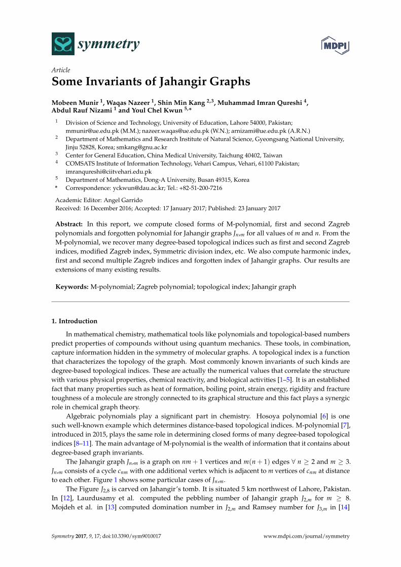
The Jahangir graph Jn,m is a graph on nm + 1 vertices and m(n + 1) edges ∀ n ≥ 2 and m ≥ 3.Jn,m consists of a cycle cnm with one additional vertex which is adjacent to m vertices of cnm at distanceto each other. Figure 1 shows some particular cases of Jn,m.

The Figure J2,8 is carved on Jahangir’s tomb. It is situated 5 km northwest of Lahore, Pakistan.In [12], Laurdusamy et al. computed the pebbling number of Jahangir graph J2,m for m ≥ 8.Mojdeh et al. in [13] computed domination number in J2,m and Ramsey number for J3,m in [14]

Symmetry 2017, 9, 17; doi:10.3390/sym9010017 www.mdpi.com/journal/symmetry

http://www.mdpi.com/journal/symmetry

http://www.mdpi.com

http://www.mdpi.com/journal/symmetry

Symmetry 2017, 9, 17 2 of 15

by Ali et al. Weiner index and Hosoya Polynomial of J2,m J3,m and J4,m are computed in [15–17].All these results are partial and need to be generalized for all values of m and n.Symmetry 2017, 9, x FOR PEER REVIEW 2 of 17

4,4J 4,5J 4,6J 4,16J 4,32J

Figure 1. The graphs of 4,4 4,5 4,6 4,16 4,32, , , , .J J J J J

The Figure 2,8J is carved on Jahangir’s tomb. It is situated 5 km northwest of Lahore,

Pakistan. In [12], Laurdusamy et al. computed the pebbling number of Jahangir graph 2,mJ for

8m ≥ . Mojdeh et al. in [13] computed domination number in 2,mJ and Ramsey number for 3,mJ

in [14] by Ali et al. Weiner index and Hosoya Polynomial of 2,mJ 3,mJ and 4,mJ are computed in

[15–17]. All these results are partial and need to be generalized for all values of m and n. In this article, we compute M-polynomial, first and second Zagreb polynomials and forgotten

polynomial of Jn,m. We also compute many degree-based topological indices for this family of the graph. We analyze these indices against parametric values m and n graphically and draw some nice conclusions as well.

Throughout this report, G is a connected graph, V(G) and E(G) are the vertex set and the edge set, respectively, and vd denotes the degree of a vertex v.

Definition 1. The M-polynomial of G is defined as [7]:

( ) ( ) , ,i j

i jijm G xM G x y y

δ ≤ ≤ ≤Δ=

where { | ( )},vMin d v V Gδ = ∈ { | ( )},vMax d v V GΔ = ∈ and ( )ijm G is the edge ( )vu E G∈

such that { } { }., ,v ud d i j=

The first topological index was introduced by Wiener [18] and it was named path number, which is now known as Wiener index. In chemical graph theory, this is the most studied molecular topological index due to its wide applications, see for details [19,20]. Randic index [21], denoted by

12

( )R G−

and introduced by Milan Randic in 1975 is also one of the oldest topological indexes. The

Randic index is defined as:

1( )2

1( ) .u vuv E G

R Gd d− ∈

=

In 1998, Ballobas and Erdos [22] and Amic et al. [23] gave an idea of generalized Randic index. This index is equally popular among chemists and mathematicians [24]. Many mathematical properties of this index have been discussed in [25]. For a detailed survey, we refer to the book [26].

The general Randic index is defined as:

( )

1( ) ,( )uv E G u v

R Gd d

α α∈

=

and the inverse Randic index is defined as ( )

( ) ( ) .u vuv E G

RR G d d αα

∈=

Figure 1. The graphs of J4,4, J4,5, J4,6, J4,16, J4,32.

In this article, we compute M-polynomial, first and second Zagreb polynomials and forgottenpolynomial of Jn,m. We also compute many degree-based topological indices for this family of thegraph. We analyze these indices against parametric values m and n graphically and draw some niceconclusions as well.

Throughout this report, G is a connected graph, V(G) and E(G) are the vertex set and the edge set,respectively, and dv denotes the degree of a vertex v.

Definition 1. The M-polynomial of G is defined as [7]:

M(G, x, y) = ∑δ≤i≤j≤∆

mij(G)xiyj

where δ = Min{dv|v ∈ V(G)}, ∆ = Max{dv|v ∈ V(G)}, and mij(G) is the edge vu ∈ E(G) such that{dv, du} = {i, j}.

The first topological index was introduced by Wiener [18] and it was named path number, which isnow known as Wiener index. In chemical graph theory, this is the most studied molecular topologicalindex due to its wide applications, see for details [19,20]. Randic index [21], denoted by R− 1

2(G) and

introduced by Milan Randic in 1975 is also one of the oldest topological indexes. The Randic index isdefined as:

R− 12(G) = ∑

uv∈E(G)

1√dudv

In 1998, Ballobas and Erdos [22] and Amic et al. [23] gave an idea of generalized Randic index.This index is equally popular among chemists and mathematicians [24]. Many mathematical propertiesof this index have been discussed in [25]. For a detailed survey, we refer to the book [26].

The general Randic index is defined as:

Rα(G) = ∑uv∈E(G)

1(dudv)

α

and the inverse Randic index is defined as RRα(G) = ∑uv∈E(G)

(dudv)α.

Obviously, R− 12(G) is the particular case of Rα(G) when α = − 1

2 .The Randic index is the most popular, most often applied and most studied among all other

topological indices. Many papers and books [27,28] are written on this topological index. Randichimself wrote two reviews on his Randic index [29,30]. The suitability of the Randic index for drugdesign was immediately recognized, and eventually, the index was used for this purpose on countlessoccasions. The physical reason for the success of such a simple graph invariant is still an enigma,although several more-or-less plausible explanations were offered.

Symmetry 2017, 9, 17 3 of 15

Gutman and Trinajstic’ introduced first Zagreb index and second Zagreb index, which are definedas: M1(G) = ∑

uv∈E(G)(du + dv) and M2(G) = ∑

uv∈E(G)(du × dv) respectively. The second modified

Zagreb index is defined as:m M2(G) = ∑

uv∈E(G)

1d(u)d(v)

For details on these indices, we refer [31–34] to the readers.The Symmetric division index is defined as:

SDD(G) = ∑uv∈E(G)

{min(du, dv)

max(du, dv)+

max(du, dv)

min(du, dv)

}

Another variant of Randic index is the harmonic index defined as:

H(G) = ∑vu∈E(G)

2du + dv

The Inverse sum-index is defined as:

I(G) = ∑vu∈E(G)

dudv

du + dv

The augmented Zagreb index is defined as:

A(G) = ∑vu∈E(G)

{dudv

du + dv − 2

}3

and it is useful for computing heat of formation of alkanes [35,36].Recently, in 2015, Furtula and Gutman introduced another topological index called forgotten

index or F-index.F(G) = ∑

uv∈E(G)

[(du)

2 + (dv)2]

We give derivations of some well-known degree-based topological indices from M-polynomial [7]in Table 1.

Table 1. Derivation of some degree-based topological indices from M-polynomial.

Topological Index Derivation from M(G; x, y)

First Zagreb(

Dx + Dy)(M(G; x, y))x=y=1

Second Zagreb(

DxDy)(M(G; x, y))x=y=1

Second Modified Zagreb(SxSy

)(M(G; x, y))x=y=1

Inverse Randic(

Dαx Dα

y

)(M(G; x, y))x=y=1

General Randic(

SαxSα

y

)(M(G; x, y))x=y=1

Symmetric Division Index(

DxSy + SxDy)(M(G; x, y))x=y=1

Harmonic Index 2Sx J(M(G; x, y))x=1

Inverse sum Index Sx JDxDy(M(G; x, y))x=1

Augmented Zagreb Index Sx3Q−2 JDx

3Dy3(M(G; x, y))x=1

Where Dx = x ∂( f (x,y)∂x , Dy = y ∂( f (x,y)

∂y , Sx =x∫

0

f (t,y)t dt, Sy =

y∫0

f (x,t)t dt, J( f (x, y)) = f (x, x), Qα( f (x, y)) = xα f (x, y).

Symmetry 2017, 9, 17 4 of 15

In 2013, Shirdel et al. in [37] proposed “hyper-Zagreb index” which is also degree based index.

Definition 2. Let G be a simple connected graph. Then the hyper-Zagreb index of G is defined as:

HM(G) = ∑uv∈E(G)

[du + dv]2

In 2012, Ghorbani and Azimi [38] proposed two new variants of Zagreb indices.

Definition 3. Let G be a simple connected graph. Then the first multiple Zagreb index of G is defined as:

PM1(G) = ∏uv∈E(G)

[du + dv]

Definition 4. Let G be a simple connected graph. Then the second multiple Zagreb index of G is defined as:

PM2(G) = ∏uv∈E(G)

[du · dv]

Definition 5. Let G be a simple connected graph. Then the first Zagreb polynomial of G is defined as:

M1(G, x) = ∑uv∈E(G)

x[du+dv ]

Definition 6. Let G be a simple connected graph. Then second Zagreb polynomial of G is defined as:

M2(G, x) = ∑uv∈E(G)

x[du ·dv ]

Definition 7. Let G be a simple connected graph. The Forgotten polynomial of G is defined as:

F(G, x) = ∑uv∈E(G)

x[(du)2+(dv)

2]

2. Main Results

In this part, we give our main computational results.

Theorem 1. Let Jn,m be the Jahangir graph. Then, the M-polynomial of Jn,m is:

M(Jn,m; x, y) = m(n− 2)x2y2 + 2mx2y3 + mx3ym

Proof. Clearly, we have |V(Jn,m)| = 8n + 2 and |E(Jn,m)| = 10n + 1. From the decision on above,we can divide the edge set into following three partitions:

E1(Jn,m) = {e = uv ∈ E(Jn,m) : du = dv = 2}

E2(Jn,m) = {e = uv ∈ E(Jn,m) : du = 2, dv = 3}

E3(Jn,m) = {e = uv ∈ E(Jn,m) : du = 3, dv = m}

In addition:|E1(Jn,m)| = m(n− 2)

Symmetry 2017, 9, 17 5 of 15

|E2(Jn,m)| = 2m

|E3(Jn,m)| = m

Now, by definition of M-polynomial, we have:

M(Jn,m; x, y) = ∑i≤j

mijxiyj

= ∑2≤2

m22x2y2 + ∑2≤3

m23x2y3 + ∑3≤m

m3mx3ym

= ∑uv∈E1(Jn,m)

m22x2y2 + ∑uv∈E2(Jn,m)

m23x2y3 + ∑uv∈E3(Jn,m)

m3mx3ym

= |E1(Jn,m)|x2y2 + |E2(Jn,m)|x2y3 + |E3(Jn,m)|x3ym

= m(n− 2)x2y2 + 2mx2y3 + mx3ym.

.

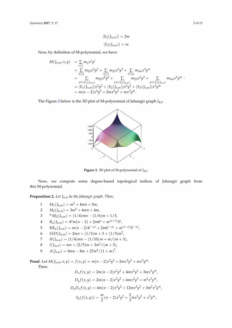
The Figure 2 below is the 3D plot of M-polynomial of Jahangir graph J4,5.

Symmetry 2017, 9, 17 5 of 16

3 , ,( ) ( ) : 3,n m n m u vE J e uv E J d d m

In addition:

1 ,( ) 2n mE J m n

2 ,( ) 2n mE J m

3 ,( )n mE J m

Now, by definition of M-polynomial, we have:

,

22 23 3

22 2

2 2 3

3

2 3

3

1 , , 3 ,2

2 2 2 3 3

2 2 2 3 3

( ) ( ) ( )

2 21 , 2 ,

? ,

( ) (

i jij

i j

m

n m

m

m

n m n m n muv E u

m

m

J Jv E uv J

n m

E

n

M x y m x y

m m

m m

J

m

m

x y x y x y

x y x y x y

J x y JE E

2 3 33 ,

2 2 2 3 3 2

) (

2

)

.

mm n m

m

E

m n

x y J x y

x y xm y x ym

The figure 2 below is the 3D plot of M-polynomial of Jahangir graph 4,5J .

Figure 2. 3D plot of M-polynomial of 4,5J .

Now, we compute some degree-based topological indices of Jahangir graph from this M-

polynomial.

Proposition 2. Let ,n mJ be the Jahangir graph. Then:

1 21 ,( ) 4 5n m mM mJ mn ,

2 2 ,23( 4 4)n m mM J mn m ,

3 2 ,( ) (1/ 4) - (1/ 6) 1/ 3mn mM J mn m ,

4 ,( 1)4 ( 2) 2 6 3a a

ma a

n m n m mR J ,

5 ( ) ( 1 ),

) ( ( )( 2)4 2 6 3a a a an m m n m mRR J ,

Figure 2. 3D plot of M-polynomial of J4,5.

Now, we compute some degree-based topological indices of Jahangir graph fromthis M-polynomial.

Proposition 2. Let Jn,m be the Jahangir graph. Then:

1 M1(Jn,m) = m2 + 4mn + 5m,2 M2(Jn,m) = 3m2 + 4mn + 4m,3 m M2(Jn,m) = (1/4)mn− (1/6)m + 1/3,

4 Rα(Jn,m) = 4am(n− 2) + 2m6a + m(a+1)3a,

5 RRα(Jn,m) = m(n− 2)4(−a) + 2m6(−a) + m(1−a)3(−a),6 SSD(Jn,m) = 2mn + (1/3)m + 3 + (1/3)m2,7 H(Jn,m) = (1/4)mn− (1/10)m + m/(m + 3),8 I(Jn,m) = mn + (2/5)m + 3m2/(m + 3),

9 A(Jn,m) = 8mn− 8m + 27m4/(1 + m)3.

Proof. Let M(Jn,m; x, y) = f (x, y) = m(n− 2)x2y2 + 2mx2y3 + mx3ym.Then:

Dx f (x, y) = 2m(n− 2)x2y2 + 4mx2y3 + 3mx3ym,

Dy f (x, y) = 2m(n− 2)x2y2 + 6mx2y3 + m2x3ym,

DyDx f (x, y) = 4m(n− 2)x2y2 + 12mx2y3 + 3m2x3ym,

Sy( f (x, y)) =m2(n− 2)x2y2 +

23

mx2y3 + x3ym,

Symmetry 2017, 9, 17 6 of 15

SxSy( f (x, y)) =m4(n− 2)x2y2 +

13

mx2y3 +13

x3ym,

Dyα( f (x, y)) = 2αm(n− 2)x2y2 + 2× 3αmx2y3 + mα+1x3ym,

DxαDy

α( f (x, y)) = 22αm(n− 2)x2y2 + 2α+1 × 3αmx2y3 + 3αmα+1x3ym

Syα( f (x, y)) =

m2α

(n− 2)x2y2 +23α

mx2y3 +mmα

x3ym,

SxαSy

α( f (x, y)) =m

22α(n− 2)x2y2 +

22α3α

mx2y3 +m

3αmαx3ym,

SyDx( f (x, y)) = m(n− 2)x2y2 +43

mx2y3 + 3x3ym,

SxDy( f (x, y)) = m(n− 2)x2y2 + 3mx2y3 +m2

3x3ym,

J f (x, y) = m(n− 2)x4 + 2mx5 + mx3+m,

Sx J f (x, y) =m4(n− 2)x4 +

25

mx5 +m

3 + mx3+m,

JDxDy f (x, y) = 4m(n− 2)x4 + 12mx5 + 3m2x3+m,

Sx JDxDy f (x, y) = m(n− 2)x4 +125

mx5 +3

3 + mm2x3+m,

Dy3 f (x, y) = 23m(n− 2)x2y2 + 2× 33mx2y3 + m4x3ym,

Dx3Dy

3 f (x, y) = 26m(n− 2)x2y2 + 24 × 33mx2y3 + 33m4x3ym,

JDx3Dy

3 f (x, y) = 26m(n− 2)x4 + 24 × 33mx5 + 33m4x3+m,

Q−2 JDx3Dy

3 f (x, y) = 26m(n− 2)x2 + 24 × 33mx3 + 33m4x1+m,

Sx3Q−2 JDx

3Dy3 f (x, y) = 23m(n− 2)x2 + 24mx3 + 33(1 + m)−3m4x1+m.

Now, from Table 1:1. First Zagreb Index

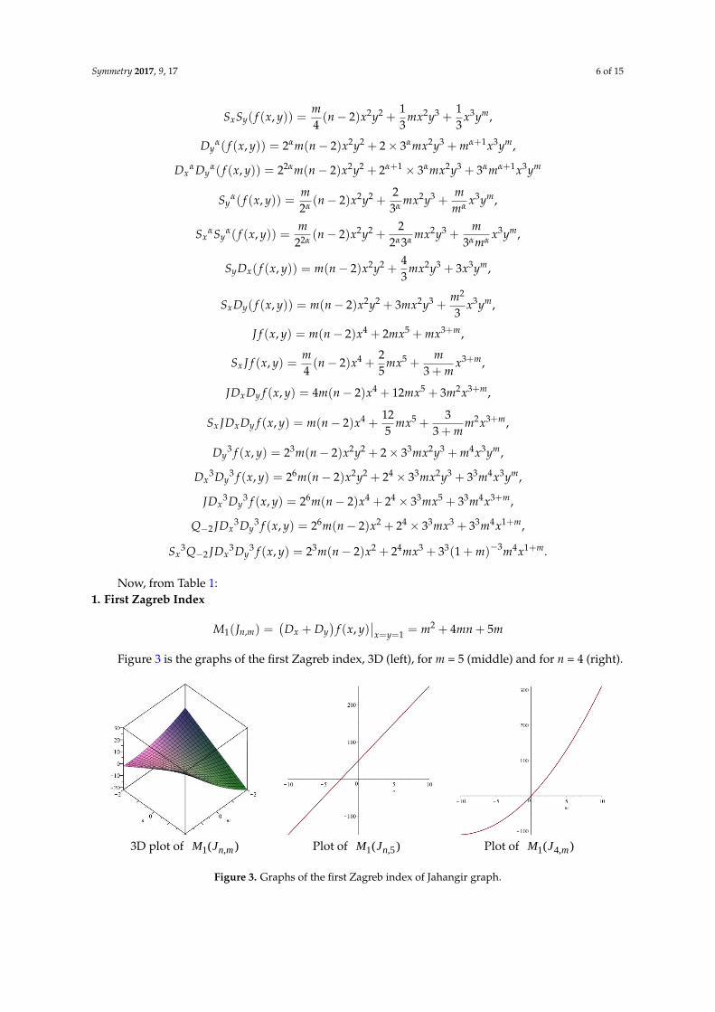
M1(Jn,m) =(

Dx + Dy)

f (x, y)∣∣x=y=1 = m2 + 4mn + 5m

Figure 3 is the graphs of the first Zagreb index, 3D (left), for m = 5 (middle) and for n = 4 (right).

Symmetry 2017, 9, 17 7 of 16

3 3 6 2 3 34 3 4 12 2 2( , ) 2 3 ,3 m

x yQ JD D f x y x xm n m xm

3 3 3 3 2 3 32

4 3 4 12( , ) 2 3 1 ) .2 ( mx x yS Q JD D f x y x xm n m mm x

Now, from Table 1:

1. First Zagreb Index

1 ,1

2( ) ( , 4 5)n m x yx y

M J D D f x y m mn m


3D plot of 1 ,( )n mM J

Plot of 1 ,5( )nM J Plot of 1 4,( )mM J

Figure 3. Graphs of the first Zagreb index of Jahangir graph.

2. Second Zagreb Index

2 , 1

2( ) ( ( , ) 3 4 .4)n m y x x ym mn mM J D D f x y

Figure 4 is the graphs of the second Zagreb index, 3D (left), for m = 5 (middle) and for n = 4 (right).



Figure 4. Graphs of the second Zagreb index of Jahangir graph.

3. Modified second Zagreb Index

2 , 1( ) ( ( , )) (1/ 4) - (1/ 6) 1/ 3m

n m x y x yM J S S f x y mn m

Figure 5 is the graphs of the modified second Zagreb index, 3D (left), for m = 5 (middle) and for n = 4

(right).


Symmetry 2017, 9, 17 7 of 15


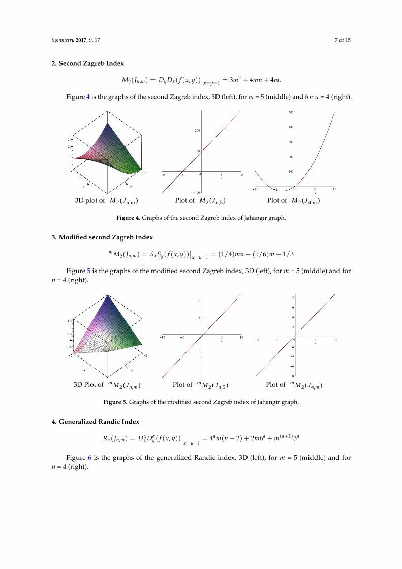
M2(Jn,m) = DyDx( f (x, y))∣∣x=y=1 = 3m2 + 4mn + 4m.


Symmetry 2017, 9, 17 7 of 16

3 3 6 2 3 34 3 4 12 2 2( , ) 2 3 ,3 m

x yQ JD D f x y x xm n m xm

3 3 3 3 2 3 32

4 3 4 12( , ) 2 3 1 ) .2 ( mx x yS Q JD D f x y x xm n m mm x

Now, from Table 1:

1. First Zagreb Index

1 ,1

2( ) ( , 4 5)n m x yx y

M J D D f x y m mn m






2 , 1

2( ) ( ( , ) 3 4 .4)n m y x x ym mn mM J D D f x y






2 , 1( ) ( ( , )) (1/ 4) - (1/ 6) 1/ 3m

n m x y x yM J S S f x y mn m

Figure 5 is the graphs of the modified second Zagreb index, 3D (left), for m = 5 (middle) and for n = 4

(right).



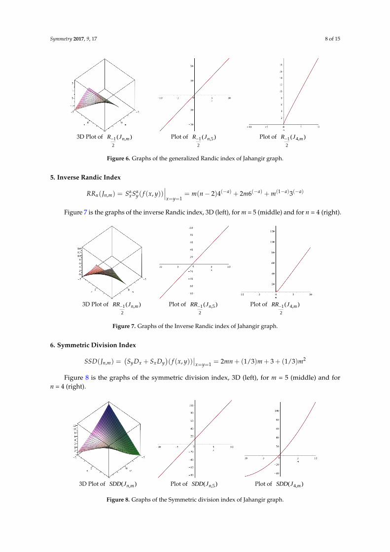
m M2(Jn,m) = SxSy( f (x, y))∣∣x=y=1 = (1/4)mn− (1/6)m + 1/3

Figure 5 is the graphs of the modified second Zagreb index, 3D (left), for m = 5 (middle) and forn = 4 (right).Symmetry 2017, 9, 17 8 of 16

3D Plot of 2 ,( )mn mM J

Plot of 2 ,5( )m

nM J Plot of 2 4,( )mmM J

Figure 5. Graphs of the modified second Zagreb index of Jahangir graph.

4. Generalized Randic Index

( )

1

1, ( ( , ) 4 ( 2) 3) 2 6a a a a

n m x yx y

R J D D f x y m n m m

Figure 6 is the graphs of the generalized Randic index, 3D (left), for m = 5 (middle) and for n = 4

(right).

3D Plot of 1 ,

2

( )n mR J Plot of 1 ,5

2

( )nR J Plot of 1 4,

2

( )mR J

Figure 6. Graphs of the generalized Randic index of Jahangir graph.

5. Inverse Randic Index

,( ) ( ) ( )

1

1 ) (( 2)4( ( , ) 6 3) 2n m x ya a a

y

a

xm n mRR J S f x mS y

Figure 7 is the graphs of the inverse Randic index, 3D (left), for m = 5 (middle) and for n = 4 (right).

3D Plot of 1 ,

2

( )n mRR J

Plot of 1 ,5

2

( )nRR J Plot of 1 4,

2

( )mRR J

Figure 7. Graphs of the Inverse Randic index of Jahangir graph.



Rα(Jn,m) = Dαx Dα

y( f (x, y))∣∣∣x=y=1

= 4am(n− 2) + 2m6a + m(a+1)3a

Figure 6 is the graphs of the generalized Randic index, 3D (left), for m = 5 (middle) and forn = 4 (right).

Symmetry 2017, 9, 17 8 of 15

Symmetry 2017, 9, 17 8 of 16


Plot of 2 ,5( )m




( )

1

1, ( ( , ) 4 ( 2) 3) 2 6a a a a

n m x yx y



(right).

3D Plot of 1 ,

2


2


2

( )mR J



,( ) ( ) ( )

1

1 ) (( 2)4( ( , ) 6 3) 2n m x ya a a

y

a



3D Plot of 1 ,

2

( )n mRR J

Plot of 1 ,5

2


2

( )mRR J

Figure 7. Graphs of the Inverse Randic index of Jahangir graph.



RRα(Jn,m) = SαxSα

y( f (x, y))∣∣∣x=y=1

= m(n− 2)4(−a) + 2m6(−a) + m(1−a)3(−a)


Symmetry 2017, 9, 17 8 of 16


Plot of 2 ,5( )m




( )

1

1, ( ( , ) 4 ( 2) 3) 2 6a a a a

n m x yx y



(right).

3D Plot of 1 ,

2


2


2

( )mR J



,( ) ( ) ( )

1

1 ) (( 2)4( ( , ) 6 3) 2n m x ya a a

y

a



3D Plot of 1 ,

2

( )n mRR J

Plot of 1 ,5

2


2

( )mRR J

Figure 7. Graphs of the Inverse Randic index of Jahangir graph. Figure 7. Graphs of the Inverse Randic index of Jahangir graph.

6. Symmetric Division Index

SSD(Jn,m) =(SyDx + SxDy

)( f (x, y))

∣∣x=y=1 = 2mn + (1/3)m + 3 + (1/3)m2

Figure 8 is the graphs of the symmetric division index, 3D (left), for m = 5 (middle) and forn = 4 (right).

Symmetry 2017, 9, 17 9 of 16


,2

12 (( 1/ 3) 3 (1/ 3)) ( , )n m y x x y

x ySSD J S D S mn mD x mf y

Figure 8 is the graphs of the symmetric division index, 3D (left), for m = 5 (middle) and for n = 4

(right).

3D Plot of ,( )n mSDD J

Plot of ,5( )nSDD J Plot of 4,( )mSDD J

Figure 8. Graphs of the Symmetric division index of Jahangir graph.

7. Harmonic Index

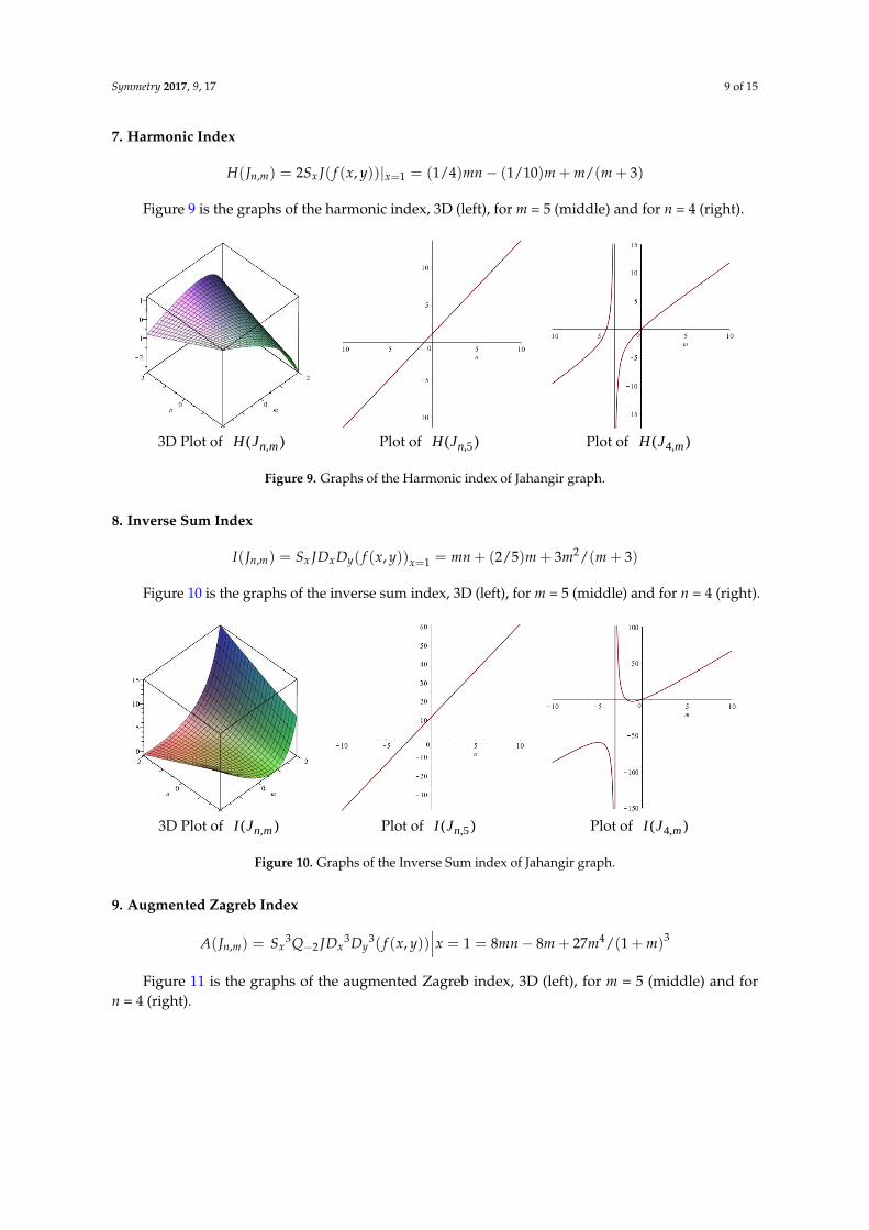
, 1 (1/ 4)2 (1/10) /( , ) ( 3| )n x xmJ J mH S f x n m my m

Figure 9 is the graphs of the harmonic index, 3D (left), for m = 5 (middle) and for n = 4 (right).

3D Plot of ,( )n mH J

Plot of ,5( )nH J Plot of 4,( )mH J

Figure 9. Graphs of the Harmonic index of Jahangir graph.

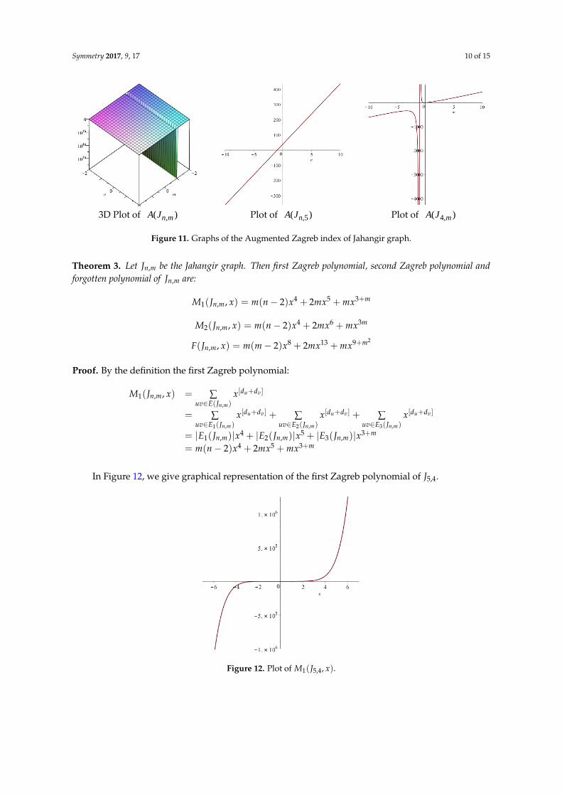
8. Inverse Sum Index

,2

1( , ) (2 / 5) 3 / ( 3)( )

xn m x x y f x yI J S JD m mD mn m

Figure 10 is the graphs of the inverse sum index, 3D (left), for m = 5 (middle) and for n = 4

(right).


Symmetry 2017, 9, 17 9 of 15

7. Harmonic Index

H(Jn,m) = 2Sx J( f (x, y))|x=1 = (1/4)mn− (1/10)m + m/(m + 3)


Symmetry 2017, 9, 17 9 of 16


,2

12 (( 1/ 3) 3 (1/ 3)) ( , )n m y x x y

x ySSD J S D S mn mD x mf y

Figure 8 is the graphs of the symmetric division index, 3D (left), for m = 5 (middle) and for n = 4

(right).

3D Plot of ,( )n mSDD J

Plot of ,5( )nSDD J Plot of 4,( )mSDD J


7. Harmonic Index

, 1 (1/ 4)2 (1/10) /( , ) ( 3| )n x xmJ J mH S f x n m my m


3D Plot of ,( )n mH J

Plot of ,5( )nH J Plot of 4,( )mH J



,2

1( , ) (2 / 5) 3 / ( 3)( )

xn m x x y f x yI J S JD m mD mn m

Figure 10 is the graphs of the inverse sum index, 3D (left), for m = 5 (middle) and for n = 4

(right).



I(Jn,m) = Sx JDxDy( f (x, y))x=1 = mn + (2/5)m + 3m2/(m + 3)

Figure 10 is the graphs of the inverse sum index, 3D (left), for m = 5 (middle) and for n = 4 (right).Symmetry 2017, 9, 17 10 of 16

3D Plot of ,( )n mI J

Plot of ,5( )nI J Plot of 4,( )mI J

Figure 10. Graphs of the Inverse Sum index of Jahangir graph.

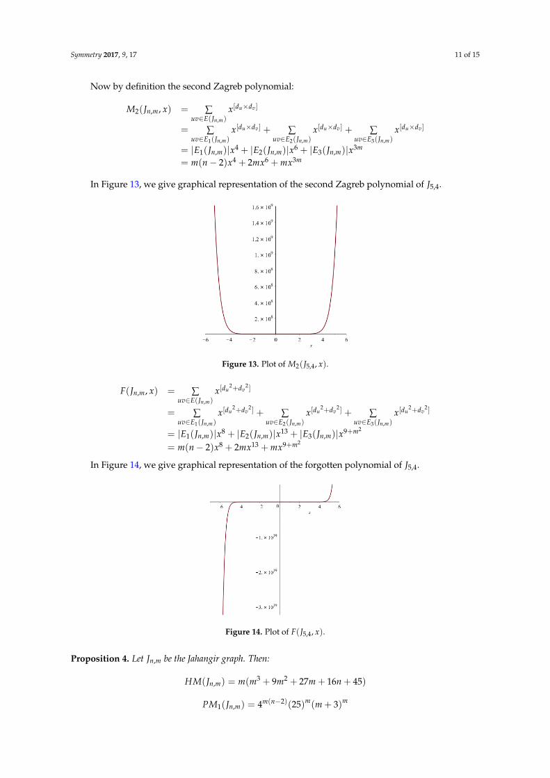
9. Augmented Zagreb Index

3 4 33 3, 2 ( , ) 1( ) 8 8 27 / (1 )n m x x y f x y x mn m m mA J S Q JD D

Figure 11 is the graphs of the augmented Zagreb index, 3D (left), for m = 5 (middle) and for n =

4 (right).

3D Plot of ,( )n mA J Plot of ,5( )nA J Plot of 4,( )mA J

Figure 11. Graphs of the Augmented Zagreb index of Jahangir graph.

Theorem 3. Let ,n mJ be the Jahangir graph. Then first Zagreb polynomial, second Zagreb polynomial and

forgotten polynomial of ,n mJ are:

4 31

5,牋 ? 2= 2 m

n mM x m nJ x mx mx

4 6 32 , , 22= m

n mM x m xnJ mx mx

28 13 9

, ( ) 2, 2mm

n m m x mx mxF J x

Proof. By the definition the first Zagreb polynomial:

,

1 , 2 , 3 ,

1

,

4 5 31 , 2 , 3 ,

4

5 3

=

= 2

,

| ?

| ?

2

u v

u v u v u

n m

n m n m n

v

m

n m

J

J J J

mn m n m n m

d d

uv E

d d d d d d

uv E uv E uv E

M x x

x x x

E x E

J

J J J

x mx mx

x E x

m n

m



A(Jn,m) = Sx3Q−2 JDx

3Dy3( f (x, y))

∣∣∣x = 1 = 8mn− 8m + 27m4/(1 + m)3

Figure 11 is the graphs of the augmented Zagreb index, 3D (left), for m = 5 (middle) and forn = 4 (right).

Symmetry 2017, 9, 17 10 of 15

Symmetry 2017, 9, 17 10 of 16

3D Plot of ,( )n mI J

Plot of ,5( )nI J Plot of 4,( )mI J



3 4 33 3, 2 ( , ) 1( ) 8 8 27 / (1 )n m x x y f x y x mn m m mA J S Q JD D

Figure 11 is the graphs of the augmented Zagreb index, 3D (left), for m = 5 (middle) and for n =

4 (right).

3D Plot of ,( )n mA J Plot of ,5( )nA J Plot of 4,( )mA J


Theorem 3. Let ,n mJ be the Jahangir graph. Then first Zagreb polynomial, second Zagreb polynomial and

forgotten polynomial of ,n mJ are:

4 31

5,牋 ? 2= 2 m

n mM x m nJ x mx mx

4 6 32 , , 22= m

n mM x m xnJ mx mx

28 13 9

, ( ) 2, 2mm

n m m x mx mxF J x


,

1 , 2 , 3 ,

1

,

4 5 31 , 2 , 3 ,

4

5 3

=

= 2

,

| ?

| ?

2

u v

u v u v u

n m

n m n m n

v

m

n m

J

J J J

mn m n m n m

d d

uv E

d d d d d d

uv E uv E uv E

M x x

x x x

E x E

J

J J J

x mx mx

x E x

m n

m


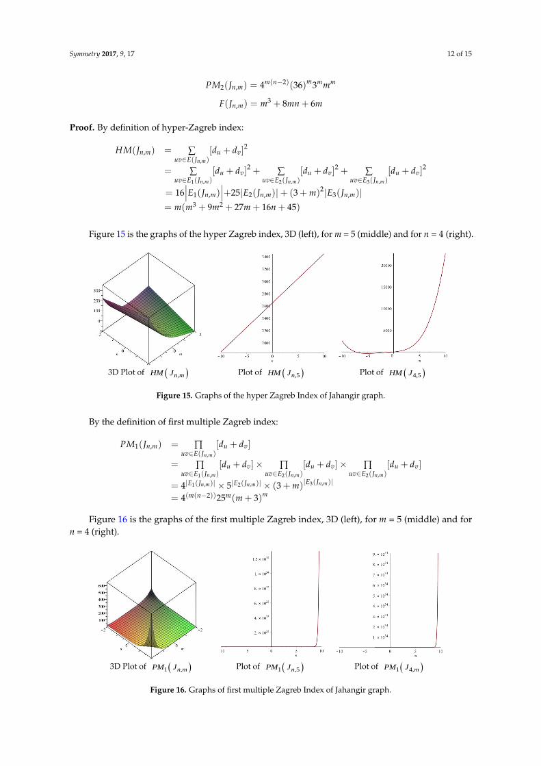
Theorem 3. Let Jn,m be the Jahangir graph. Then first Zagreb polynomial, second Zagreb polynomial andforgotten polynomial of Jn,m are:

M1(Jn,m, x) = m(n− 2)x4 + 2mx5 + mx3+m

M2(Jn,m, x) = m(n− 2)x4 + 2mx6 + mx3m

F(Jn,m, x) = m(m− 2)x8 + 2mx13 + mx9+m2


M1(Jn,m, x) = ∑uv∈E(Jn,m)

x[du+dv ]

= ∑uv∈E1(Jn,m)

x[du+dv ] + ∑uv∈E2(Jn,m)

x[du+dv ] + ∑uv∈E3(Jn,m)

x[du+dv ]

= |E1(Jn,m)|x4 + |E2(Jn,m)|x5 + |E3(Jn,m)|x3+m

= m(n− 2)x4 + 2mx5 + mx3+m

In Figure 12, we give graphical representation of the first Zagreb polynomial of J5,4.

Symmetry 2017, 9, 17 11 of 16

In Figure 12, we give graphical representation of the first Zagreb polynomial of 5,4牋 .J

Figure 12. Plot of 5,41 牋 ,M J x .

Now by definition the second Zagreb polynomial:

,

1 , 2 , 3 ,

2 ,

4 6 31 , 2 , 3 ,

4 6 3

=

,

| ?

| ?

2 = 2

u v

u

n m

n m n

v u v u v

m n m

d d

uv E

d d d d d d

uv E uv E uv E

n m

J

J J J

mn m n m n m

m

M x x

x x x

E x E x E x

J

J J J

x mx mm n x

In Figure 13, we give graphical representation of the second Zagreb polynomial of 5,4牋 .J

Figure 13. Plot of 2 5,4牋 ,JM x .

,

1 , 2 ,

2 2

2 2 2 2 2

3

2

,

2

,

13 91 , 2 ,

83 ,

=

,

| ?

| ?

u v

n

u v u v u

m

n m n m n m

v

n md d

uv E

d

J

J J J

d d d d d

uv E u

mn m n m n m

v E uv E

J

J J J

F x x

x x x

E x E x E x

28 13 9 2 = 2 mx mxm n mx

Figure 12. Plot of M1(J5,4, x).

Symmetry 2017, 9, 17 11 of 15


M2(Jn,m, x) = ∑uv∈E(Jn,m)

x[du×dv ]

= ∑uv∈E1(Jn,m)

x[du×dv ] + ∑uv∈E2(Jn,m)

x[du×dv ] + ∑uv∈E3(Jn,m)

x[du×dv ]

= |E1(Jn,m)|x4 + |E2(Jn,m)|x6 + |E3(Jn,m)|x3m

= m(n− 2)x4 + 2mx6 + mx3m

In Figure 13, we give graphical representation of the second Zagreb polynomial of J5,4.

Symmetry 2017, 9, 17 11 of 16

In Figure 12, we give graphical representation of the first Zagreb polynomial of 5,4牋 .J

Figure 12. Plot of 5,41 牋 ,M J x .


,

1 , 2 , 3 ,

2 ,

4 6 31 , 2 , 3 ,

4 6 3

=

,

| ?

| ?

2 = 2

u v

u

n m

n m n

v u v u v

m n m

d d

uv E

d d d d d d

uv E uv E uv E

n m

J

J J J

mn m n m n m

m

M x x

x x x

E x E x E x

J

J J J

x mx mm n x

In Figure 13, we give graphical representation of the second Zagreb polynomial of 5,4牋 .J

Figure 13. Plot of 2 5,4牋 ,JM x .

,

1 , 2 ,

2 2

2 2 2 2 2

3

2

,

2

,

13 91 , 2 ,

83 ,

=

,

| ?

| ?

u v

n

u v u v u

m

n m n m n m

v

n md d

uv E

d

J

J J J

d d d d d

uv E u

mn m n m n m

v E uv E

J

J J J

F x x

x x x

E x E x E x

28 13 9 2 = 2 mx mxm n mx

Figure 13. Plot of M2(J5,4, x).

F(Jn,m, x) = ∑uv∈E(Jn,m)

x[du2+dv

2]

= ∑uv∈E1(Jn,m)

x[du2+dv

2] + ∑uv∈E2(Jn,m)

x[du2+dv

2] + ∑uv∈E3(Jn,m)

x[du2+dv

2]

= |E1(Jn,m)|x8 + |E2(Jn,m)|x13 + |E3(Jn,m)|x9+m2

= m(n− 2)x8 + 2mx13 + mx9+m2

In Figure 14, we give graphical representation of the forgotten polynomial of J5,4.

Symmetry 2017, 9, 17 12 of 16

In Figure 14, we give graphical representation of the forgotten polynomial of 5,4牋 .J

Figure 14. Plot of 5,4牋 ,JF x .


,3 2( ) ( 9 27 16 45)n mH JM m m m m n

,( 2)

1 4 25 ( 3)mm n

n mmPM mJ

(2 ,

2) 4 36 3mn

mn m mmPM mJ

3,( 6) 8n m mF mJ mn

Proof. By definition of hyper-Zagreb index:

2

2 2 2

,

,

1 , 2 , 3 ,

1 , 22

3

,

2

3 ,

16 | ? | 25 ? 3 ?

= ( 9 27 16

45)

u v

uv E

u v u v u v

n m

Jn m

J J Jn m n m n m

n m n

uv

m n

E uv E uv E

m

HM d d

d d d d d d

E E m

J

J J E

m m m m n

J

Figure 15 is the graphs of the hyper Zagreb index, 3D (left), for m = 5 (middle) and for n = 4

(right).

3D Plot of , n mHM J Plot of ,5 nHM J Plot of 4,5 HM J

Figure 15. Graphs of the hyper Zagreb Index of Jahangir graph.

Figure 14. Plot of F(J5,4, x).

Proposition 4. Let Jn,m be the Jahangir graph. Then:

HM(Jn,m) = m(m3 + 9m2 + 27m + 16n + 45)

PM1(Jn,m) = 4m(n−2)(25)m(m + 3)m

Symmetry 2017, 9, 17 12 of 15

PM2(Jn,m) = 4m(n−2)(36)m3mmm

F(Jn,m) = m3 + 8mn + 6m


HM(Jn,m) = ∑uv∈E(Jn,m)

[du + dv]2

= ∑uv∈E1(Jn,m)

[du + dv]2 + ∑

uv∈E2(Jn,m)[du + dv]

2 + ∑uv∈E3(Jn,m)

[du + dv]2

= 16∣∣∣E1(Jn,m)

∣∣∣+25|E2(Jn,m)|+ (3 + m)2|E3(Jn,m)|= m(m3 + 9m2 + 27m + 16n + 45)

Figure 15 is the graphs of the hyper Zagreb index, 3D (left), for m = 5 (middle) and for n = 4 (right).

Symmetry 2017, 9, 17 12 of 16

In Figure 14, we give graphical representation of the forgotten polynomial of 5,4牋 .J

Figure 14. Plot of 5,4牋 ,JF x .


,3 2( ) ( 9 27 16 45)n mH JM m m m m n

,( 2)

1 4 25 ( 3)mm n

n mmPM mJ

(2 ,

2) 4 36 3mn

mn m mmPM mJ

3,( 6) 8n m mF mJ mn


2

2 2 2

,

,

1 , 2 , 3 ,

1 , 22

3

,

2

3 ,

16 | ? | 25 ? 3 ?

= ( 9 27 16

45)

u v

uv E

u v u v u v

n m

Jn m

J J Jn m n m n m

n m n

uv

m n

E uv E uv E

m

HM d d

d d d d d d

E E m

J

J J E

m m m m n

J

Figure 15 is the graphs of the hyper Zagreb index, 3D (left), for m = 5 (middle) and for n = 4

(right).

3D Plot of , n mHM J Plot of ,5 nHM J Plot of 4,5 HM J

Figure 15. Graphs of the hyper Zagreb Index of Jahangir graph. Figure 15. Graphs of the hyper Zagreb Index of Jahangir graph.

By the definition of first multiple Zagreb index:

PM1(Jn,m) = ∏uv∈E(Jn,m)

[du + dv]

= ∏uv∈E1(Jn,m)

[du + dv]× ∏uv∈E2(Jn,m)

[du + dv]× ∏uv∈E2(Jn,m)

[du + dv]

= 4|E1(Jn,m)| × 5|E2(Jn,m)| × (3 + m)|E3(Jn,m)|

= 4(m(n−2))25m(m + 3)m

Figure 16 is the graphs of the first multiple Zagreb index, 3D (left), for m = 5 (middle) and forn = 4 (right).

Symmetry 2017, 9, 17 13 of 16


,

,

1 , 2 , 2 ,

2 ,

1

| 3 , |

( )

1

(

,

2 )

4 5 (3 )

=4 25 ( 3)

n m

Jn m

J J Jn m n m n m

J JJ n m n

u v

uv E

u v u v u v

uv E uv E uv E

E EE

m n m m

mn m

PM d d

d d d d d d

J

m

m

Figure 16 is the graphs of the first multiple Zagreb index, 3D (left), for m = 5 (middle) and for n

= 4 (right).

3D Plot of 1 , n mPM J Plot of ,51 nPM J Plot of 4,1 mPM J

Figure 16. Graphs of first multiple Zagreb Index of Jahangir graph.

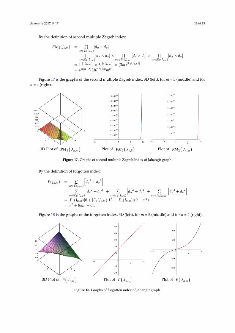
By the definition of second multiple Zagreb index:

| ?

|

2 ,

,

1 , 2 , 2 ,

2 , 3 ,1 ,

( 2)

4 6 (3

=

)

4 36 3

n m

Jn m

J J Jn m n m n m

J JJ n m n mn

u v

uv E

u v u v u v

uv E uv E uv E

E EmE

mm n m m

PM d d

d d d d d d

J

m

m

Figure 17 is the graphs of the second multiple Zagreb index, 3D (left), for m = 5 (middle) and for

n = 4 (right).

3D Plot of 2 , n mPM J

Plot of 2 ,5 nPM J Plot of 2 4, mPM J

Figure 17. Graphs of second multiple Zagreb Index of Jahangir graph.


Symmetry 2017, 9, 17 13 of 15


PM2(Jn,m) = ∏uv∈E(Jn,m)

[du × dv]

= ∏uv∈E1(Jn,m)

[du × dv]× ∏uv∈E2(Jn,m)

[du × dv]× ∏uv∈E2(Jn,m)

[du × dv]

= 4|E1(Jn,m)| × 6|E2(Jn,m)| × (3m)|E3(Jn,m)|

= 4m(n−2)(36)m3mmm

Figure 17 is the graphs of the second multiple Zagreb index, 3D (left), for m = 5 (middle) and forn = 4 (right).

Symmetry 2017, 9, 17 13 of 16


,

,

1 , 2 , 2 ,

2 ,

1

| 3 , |

( )

1

(

,

2 )

4 5 (3 )

=4 25 ( 3)

n m

Jn m

J J Jn m n m n m

J JJ n m n

u v

uv E

u v u v u v

uv E uv E uv E

E EE

m n m m

mn m

PM d d

d d d d d d

J

m

m

Figure 16 is the graphs of the first multiple Zagreb index, 3D (left), for m = 5 (middle) and for n

= 4 (right).

3D Plot of 1 , n mPM J Plot of ,51 nPM J Plot of 4,1 mPM J



| ?

|

2 ,

,

1 , 2 , 2 ,

2 , 3 ,1 ,

( 2)

4 6 (3

=

)

4 36 3

n m

Jn m

J J Jn m n m n m

J JJ n m n mn

u v

uv E

u v u v u v

uv E uv E uv E

E EmE

mm n m m

PM d d

d d d d d d

J

m

m

Figure 17 is the graphs of the second multiple Zagreb index, 3D (left), for m = 5 (middle) and for

n = 4 (right).

3D Plot of 2 , n mPM J

Plot of 2 ,5 nPM J Plot of 2 4, mPM J

Figure 17. Graphs of second multiple Zagreb Index of Jahangir graph. Figure 17. Graphs of second multiple Zagreb Index of Jahangir graph.

By the definition of forgotten index:

F(Jn,m) = ∑uv∈E(Jn,m)

[du

2 + dv2]

= ∑uv∈E1(Jn,m)

[du

2 + dv2]+ ∑

uv∈E2(Jn,m)

[du

2 + dv2]+ ∑

uv∈E3(Jn,m)

[du

2 + dv2]

= |E1(Jn,m)|8 + |E2(Jn,m)|13 + |E3(Jn,m)|(9 + m2)

= m3 + 8mn + 6m

Figure 18 is the graphs of the forgotten index, 3D (left), for m = 5 (middle) and for n = 4 (right).

Symmetry 2017, 9, 17 14 of 16

By the definition of F-index:

,

1 , 2 , 3 ,

,

1 , 2 , 3 ,

2 2

2 2 2 2 2 2

2

=

| ?

| 8 ?

13 ? (9

)

n m

n m n m n m

u v

uv E

u v u v u v

uv E uv E uv

n m

J

J J J

n m n m n

E

m

F d d

d d d d d d

E E E m

J

J J J

3= 8 6m mn m

Figure 18 is the graphs of the F-index, 3D (left), for m = 5 (middle) and for n = 4 (right).

3D Plot of , n mF J Plot of ,5 nF J Plot of 4, mF J

Figure 18. Graphs of forgotten index (F-index) of Jahangir graph.

It is worth mentioning that above-plotted surfaces and graphs show the dependence of each

topological index on m and n. From these figures, one can imagine that each topological index

behaves differently from other against parameters m and n. These figures also give us some extreme

values of the certain topological index. Moreover, these graphs give an insight view to control the

values of topological indices with m and n.

3. Conclusions and Discussion

In this article, we computed closed forms of many topological indices and polynomials of ,n mJ

for all values of m and n. These facts are invariants of graphs and remain preserved under

isomorphism. These results can also play a vital role in industry and pharmacy in the realm of that

molecular graph which contains ,n mJ as its subgraphs.

Acknowledgments: This research is supported by Gyeongsang National University, Jinju 52828, Korea.

Author Contributions: Mobeen Munir, Waqas Nazeer, Shin Min Kang, Muhammad Imran Qureshi, Abdul Rauf

Nizami and Youl Chel Kwun contribute equally in writing of this article.

Conflicts of Interest: The authors declare no conflict of interest.

References

1. Rücker, G.; Rücker, C. On topological indices, boiling points, and cycloalkanes. J. Chem. Inf. Comput. Sci.

1999, 39, 788–802.

2. Klavzar, S.; Gutman, I. A comparison of the Schultz molecular topological index with the Wiener index. J.

Chem. Inf. Comput. Sci. 1996, 36, 1001–1003.

3. Brückler, F.M.; Došlić, T.; Graovac, A.; Gutman, I. On a class of distance-based molecular structure

descriptors. Chem. Phys. Lett. 2011, 503, 336–338.

4. Deng, H.; Yang, J.; Xia, F. A general modeling of some vertex-degree based topological indices in benzenoid

systems and phenylenes. Comput. Math. Appl. 2011, 61, 3017–3023.

Figure 18. Graphs of forgotten index of Jahangir graph.

Symmetry 2017, 9, 17 14 of 15

It is worth mentioning that above-plotted surfaces and graphs show the dependence of eachtopological index on m and n. From these figures, one can imagine that each topological index behavesdifferently from other against parameters m and n. These figures also give us some extreme valuesof the certain topological index. Moreover, these graphs give an insight view to control the values oftopological indices with m and n.

3. Conclusions and Discussion

In this article, we computed closed forms of many topological indices and polynomials of Jn,m forall values of m and n. These facts are invariants of graphs and remain preserved under isomorphism.These results can also play a vital role in industry and pharmacy in the realm of that molecular graphwhich contains Jn,m as its subgraphs.

Acknowledgments: This research is supported by Gyeongsang National University, Jinju 52828, Korea.

Author Contributions: Mobeen Munir, Waqas Nazeer, Shin Min Kang, Muhammad Imran Qureshi, Abdul RaufNizami and Youl Chel Kwun contribute equally in writing of this article.

Conflicts of Interest: The authors declare no conflict of interest.

References

1. Rücker, G.; Rücker, C. On topological indices, boiling points, and cycloalkanes. J. Chem. Inf. Comput. Sci.1999, 39, 788–802. [CrossRef]

2. Klavzar, S.; Gutman, I. A comparison of the Schultz molecular topological index with the Wiener index.J. Chem. Inf. Comput. Sci. 1996, 36, 1001–1003. [CrossRef]

3. Brückler, F.M.; Došlic, T.; Graovac, A.; Gutman, I. On a class of distance-based molecular structure descriptors.Chem. Phys. Lett. 2011, 503, 336–338. [CrossRef]

4. Deng, H.; Yang, J.; Xia, F. A general modeling of some vertex-degree based topological indices in benzenoidsystems and phenylenes. Comput. Math. Appl. 2011, 61, 3017–3023. [CrossRef]

5. Zhang, H.; Zhang, F. The Clar covering polynomial of hexagonal systems I. Discret. Appl. Math. 1996, 69,147–167. [CrossRef]

6. Gutman, I. Some properties of the Wiener polynomials. Graph Theory Notes N. Y. 1993, 125, 13–18.7. Deutsch, E.; Klavzar, S. M-Polynomial, and degree-based topological indices. Iran. J. Math. Chem. 2015, 6,

93–102.8. Munir, M.; Nazeer, W.; Rafique, S.; Kang, S.M. M-polynomial and related topological indices of Nanostar

dendrimers. Symmetry 2016, 8, 97. [CrossRef]9. Munir, M.; Nazeer, W.; Rafique, S.; Kang, S.M. M-Polynomial and Degree-Based Topological Indices of

Polyhex Nanotubes. Symmetry 2016, 8, 149. [CrossRef]10. Munir, M.; Nazeer, W.; Rafique, S.; Nizami, A.R.; Kang, S.M. Some Computational Aspects of Triangular

Boron Nanotubes. Symmetry 2016, 9, 6. [CrossRef]11. Munir, M.; Nazeer, W.; Shahzadi, Z.; Kang, S.M. Some invariants of circulant graphs. Symmetry 2016, 8, 134.

[CrossRef]12. Lourdusamy, A.; Jayaseelan, S.S.; Mathivanan, T. On pebbling Jahangir graph. Gen. Math. Notes 2011, 5,

42–49.13. Mojdeh, M.A.; Ghameshlou, A.N. Domination in Jahangir Graph J2,m. Int. J. Contemp. Math. Sci. 2007, 2,

1193–1199. [CrossRef]14. Ali, K.; Baskoro, E.T.; Tomescu, I. On the Ramsey number of Paths and Jahangir, graph J3,m. In Proceedings

of the 3rd International Conference on 21st Century Mathematics, Lahore, Pakistan, 4–7 March 2007.15. Farahani, M.R. Hosoya Polynomial and Wiener Index of Jahangir graphs J2,m. Pac. J. Appl. Math. 2015, 7,

221–224.16. Farahani, M.R. The Wiener Index and Hosoya polynomial of a class of Jahangir graphs J3,m. Fundam. J. Math.

Math. Sci. 2015, 3, 91–96.17. Wang, S.; Farahani, M.R.; Kanna, M.R.; Jamil, M.K.; Kumar, R.P. The Wiener Index and the Hosoya Polynomial

of the Jahangir Graphs. Appl. Comput. Math. 2016, 5, 138–141. [CrossRef]

http://dx.doi.org/10.1021/ci9900175

http://dx.doi.org/10.1021/ci9603689

http://dx.doi.org/10.1016/j.cplett.2011.01.033

http://dx.doi.org/10.1016/j.camwa.2011.03.089

http://dx.doi.org/10.1016/0166-218X(95)00081-2

http://dx.doi.org/10.3390/sym8090097




http://dx.doi.org/10.12988/ijcms.2007.07122

http://dx.doi.org/10.1016/j.cam.2015.12.007

Symmetry 2017, 9, 17 15 of 15

18. Wiener, H. Structural determination of paraffin boiling points. J. Am. Chem. Soc. 1947, 69, 17–20. [CrossRef][PubMed]

19. Dobrynin, A.A.; Entringer, R.; Gutman, I. Wiener index of trees: Theory and applications. Acta Appl. Math.2001, 66, 211–249. [CrossRef]

20. Gutman, I.; Polansky, O.E. Mathematical Concepts in Organic Chemistry; Springer Science & Business Media:New York, NY, USA, 2012.

21. Randic, M. Characterization of molecular branching. J. Am. Chem. Soc. 1975, 97, 6609–6615. [CrossRef]22. Bollobás, B.; Erdos, P. Graphs of extremal weights. Ars Comb. 1998, 50, 225–233. [CrossRef]23. Amic, D.; Bešlo, D.; Lucic, B.; Nikolic, S.; Trinajstic, N. The vertex-connectivity index revisited. J. Chem. Inf.

Comput. Sci. 1998, 38, 819–822. [CrossRef]24. Hu, Y.; Li, X.; Shi, Y.; Xu, T.; Gutman, I. On molecular graphs with smallest and greatest zeroth-order general

Randic index. MATCH Commun. Math. Comput. Chem. 2005, 54, 425–434.25. Caporossi, G.; Gutman, I.; Hansen, P.; Pavlovic, L. Graphs with maximum connectivity index.

Comput. Biol. Chem. 2003, 27, 85–90. [CrossRef]26. Li, X.; Gutman, I. Mathematical Aspects of Randic-Type Molecular Descriptors; University of Kragujevac and

Faculty of Science Kragujevac: Kragujevac, Serbia, 2006.27. Kier, L.B.; Hall, L.H. Molecular Connectivity in Chemistry and Drug Research; Academic Press: New York, NY,

USA, 1976.28. Kier, L.B.; Hall, L.H. Molecular Connectivity in Structure-Activity Analysis; Wiley: New York, NY, USA, 1986.29. Randic, M. On history of the Randic index and emerging hostility toward chemical graph theory.

MATCH Commun. Math. Comput. Chem. 2008, 59, 5–124.30. Randic, M. The connectivity index 25 years after. J. Mol. Graph. Model. 2001, 20, 19–35. [CrossRef]31. Nikolic, S.; Kovacevic, G.; Milicevic, A.; Trinajstic, N. The Zagreb indices 30 years after. Croat. Chem. Acta

2003, 76, 113–124.32. Gutman, I.; Das, K.C. The first Zagreb index 30 years after. MATCH Commun. Math. Comput. Chem. 2004, 50,

83–92.33. Das, K.C.; Gutman, I. Some properties of the second Zagreb index. MATCH Commun. Math. Comput. Chem.

2004, 52, 103–112.34. Trinajstic, N.; Nikolic, S.; Milicevic, A.; Gutman, I. On Zagreb indices. Kem. Ind. 2010, 59, 577–589.35. Huang, Y.; Liu, B.; Gan, L. Augmented Zagreb Index of Connected Graphs. MATCH Commun. Math.

Comput. Chem. 2012, 67, 483–494.36. Furtula, B.; Graovac, A.; Vukicevic, D. Augmented Zagreb index. J. Math. Chem. 2010, 48, 370–380. [CrossRef]37. Shirdel, G.H.; Pour, H.R.; Sayadi, A.M. The hyper-Zagreb index of graph operations. Iran. J. Math. Chem.

2013, 4, 213–220.38. Ghorbani, M.; Azimi, N. Note on multiple Zagreb indices. Iran. J. Math. Chem. 2012, 3, 137–143.

© 2017 by the authors; licensee MDPI, Basel, Switzerland. This article is an open accessarticle distributed under the terms and conditions of the Creative Commons Attribution(CC BY) license (http://creativecommons.org/licenses/by/4.0/).

http://dx.doi.org/10.1021/ja01193a005

http://www.ncbi.nlm.nih.gov/pubmed/20291038

http://dx.doi.org/10.1023/A:1010767517079

http://dx.doi.org/10.1021/ja00856a001

http://dx.doi.org/10.1016/S0012-365X(98)00320-3

http://dx.doi.org/10.1021/ci980039b

http://dx.doi.org/10.1016/S0097-8485(02)00016-5

http://dx.doi.org/10.1016/S1093-3263(01)00098-5

http://dx.doi.org/10.1007/s10910-010-9677-3

http://creativecommons.org/

http://creativecommons.org/licenses/by/4.0/.

Documents

Some Invariants of Jahangir Graphs - Semantic Scholar