ISSC 2009, Dublin, June 10-11

Some remarks on the well-posedness of the EMD algorithm

Konstantinos Drakakis*, Nikolaos Tsakalozost, and Scott Rickard:!:

UCD CASL University College Dublin

Belfield, Dublin 4 Ireland

E-mail: *Konstantinos.Drakakis@ucd.ie tNikolaos.Tsakalozos@gmail.com +Scott.Rickard@ucd.ie

Abstract - We identify two major difficulties with the formulation of a rigorous math­ematical theory for the Empirical Mode Decomposition (EMD): a) the concept of the envelope is not well defined, and b) the output of the EMD fails a very simple consistency criterion.

Keywords - Empirical Mode Decomposition (EMD), Intrinsic Mode Functions (IMFs), envelope, input-output consistency, output-output consistency.

I INTRODUCTION Smooth and periodic real functions defined on IR can be expanded into a Fourier series of sines and cosines whose frequencies are integral multiples of a fundamental frequency, indeed the inverse length of the period. The two main and frequently de­sirable features of this expansion are a) that the expansion functions are orthogonal to each other, and b) that the set of functions over which the expansion takes place is chosen before the func­tion being expanded. Thus, sines and cosines form a "dictionary" over which functions can be loss­lessly compressed: objects that technically need an uncountable infinity of values in order to be fully specified can now be codified through a countable infinity of (or even finitely many) real numbers, namely the coefficients of the trigonometric func­tions, without any loss of information.

This representation has its downsides, though. Consider a pure sine function y(t) = sin(27l'ft), whose Fourier expansion trivially contains one term, and consider further its slight perturbations (1 + f(t)) sin(27l' ft) and sin(27l' f(l + f( t) )t), where f (t) is a function taking "small" values and such that the two perturbations are still periodic of the same period as y. Because of the inflexibility of the trigonometric dictionary, which is chosen be­fore, and without any reference to, the function y, either perturbation will lead to an expansion con­taining infinitely many terms, despite both being so similar to y.

There are occasions where the orthogonality of the terms of the expansion is of no practical inter­est to us, and where the convenience of a fixed and a priori chosen dictionary is less important than

the sparsity and flexibility of the expansion (e.g. in dealing with non-stationarity). Besides, choos­ing the expansion terms after choosing the func­tion to be expanded carries the extra benefit that the expansion terms can contain useful informa­tion about the function, which, otherwise, would be spread over a large number of expansion terms and thus possibly lost.

The Empirical Mode Decomposition (EMD) is a relatively recently proposed algorithm, formulated by N. Huang et al. [5] in 1998, specifically address­ing these concerns. Given a function, it produces a "Fourier-like" expansion over "trigonometric-like" functions constructed out of the function f itself, called Intrinsic Mode Functions (IMFs); in fact, the class of IMFs contains all trigonometric func­tions but is significantly more general, and this extension of the set over which expansion terms are chosen leads to sparser expansions. Moreover, the IMFs have indeed been shown to contain use­ful information about the function in a variety of contexts and occasions [1, 4, 5, 11] .

The downside of the EMD is its empirical na­ture: despite the efforts of several researchers [5, 6, 10, 12] , it remains an exclusively empirical al­gorithm without a solid mathematical foundation. The part that seems to defy rigorous study the most is the concept of the envelope of a function, which is currently not completely and unambigu­ously specified. In this work we revisit the issue of the envelope, discussing how currently known en­velopes either adhere to the defining axioms or be­have well in practice, but unfortunately not both. We also touch for the first time the issue of the consistency of the algorithm, namely the fact that,

when the EMD gets applied to a sum of IMFs, it should consistently return those IMFs again as its output: this sounds almost obvious, and yet it is not clear that EMD complies with this condition.

II DESCRIPTION OF THE EMD Let f be a continuous and smooth real-valued func­tion defined on a finite closed interval D c lR with a finite number of local minima and maxima; in what follows, it will be convenient not to count the endpoints of D amongst the local minima and maxima, but treat them separately. The EMD produces functions fi, i = 1, . . . , Nand r, N be­ing determined by the algorithm and not known a priori, such that

N

f = Lfi +r. (1) i=l

The functions fi' i = 1, . . . , N are the IMFs of f and are oscillatory in nature, while r, which does not perform a full oscillation over D (namely it either has at most one maximum or at most one minimum over D), is known as the trend of f.

The EMD relies crucially upon the extraction of the envelope of f. We proceed to discuss this con­cept first, before we offer more details about the algorithm itself and its end product, the IMFs and the trend. Henceforth, unless otherwise stated, we will assume that all functions we deal with are con­tinuous and smooth.

a) Envelopes

Definition 1. The envelope of a function f de­fined as above consists of two functions, the upper envelope fu and the lower envelope fl' which are required to satisfy the following conditions:

• Vx E D, fl(X) ::; f(x) ::; fu(x). • fu(x) = f(x) whenever x is a local maximum

of f, and similarly fl(X) = f(x) whenever x is a local minimum of f.

• Whenever Xl < X2 are two consecutive local maxima, fu(x) must lie between fu(xt) and fu(X2) for all X E [XI, X2] ; similarly, whenever Xl < X2 are two consecutive local minima, fl(X) must lie between fl(Xt) and fl(X2) for all X E [XI, X2] .

In practice, the first condition is only (required to be) satisfied in an approximate sense, while the third safeguards against the choice of envelopes that assume unreasonably high or low values, and, to the best of our knowledge, has not been ex­plicitly proposed elsewhere, though envelope con­structions used in practice seem to satisfy it (again at least in an approximate sense). These con­ditions are clearly not sufficient to specify the envelope of f uniquely and unambiguously, al­though there currently seems to be some consen­sus in the literature about a preferred construc­tion method, namely the cubic spline interpolation [4, 5, 6, 10, 11] . Indeed, the second condition sug­gests that the envelope construction method can be an interpolation method relying only on the po­sitions of the local minima and maxima of f, on the endpoints of D, and on the values of f at these points. In other words, letting U(J) and L(J) be the positions of the local maxima and minima of f, respectively, and D = [db d2], we may set:

fu = L.u(U(J),f(U(J)),dl,d2,f(dl),f(d2)), fl = L.l(L(J),f(L(J)),dl,d2,f(dl),f(d2)), (2)

where L.u and L.l are two (possibly different) in­terpolation laws producing functions defined over the entire D out of the finite sets of points passed to them as their arguments. The envelope al­lows us, in turn, to define the local mean of f as l = (Ju + fl)/2. b) IMFs

IMFs [5, 12] can be construed as generalized sines, as they share indeed key characteristics with sines. In particular, they can be though of as sines with "variable width" and "fluctuating frequency" . The following definition is inspired by [14] :

Definition 2 (Intrinsic Mode Function). f de­fined on D is an Intrinsic Mode Function (IMF) if and only if there exist functions m non-negative and ¢, and reals a ::; b (either of them allowed to be ±oo but not both) such that: f(x) = m(x) cos(¢(x)), X E D, (3) ----where supp( m) c [a, b] , and supp( cos( ¢)) c lR\ [-b, -a] , A denoting the Fourier transform. In particular, m is called the envelope and ¢ the phase of the IMF. Remark 1. IMFs are the only functions for which a rigorous mathematical definition of the envelope has been given [10] . The Hilbert transform 1t [5, 14] of f as defined above can be shown, using the Bedrosian equality, to be [14] : 1t(m cos(¢)) = m1t(cos(¢)) = m sin(¢), (4) whence the analytic signal of f becomes f + i1t(J) = m exp(i¢), and the upper/lower enve­lope fu/ fl of f can be defined as the ampli­tude/negative amplitude of the analytic signal, re­spectively: f u = m, fl = -m. It follows that the local mean of an IMF is O. To the best of our understanding, however, though the spectral conditions given in Definition 2 are sufficient for Bedrosian's equality to apply, it is still not known whether they are necessary.

IMFs are usually defined [5, 10, 12] in a simpler, imprecise, yet intuitive way as functions having the following two properties:

Definition 3 (Alternative IMF definition).

• All local maxima are positive, all local minima are negative, and between any two consecutive extrema (a maximum and a minimum) lies ex­actly one zero (remember that here we do not count the endpoints as local extrema).

• The local mean is O.

Is this equivalent to Definition 2? It is relatively simple to show that an IMF as per Definition 2 satisfies both properties given in Definition 3, but, although it is clear that a function f satisfying both conditions given in Definition 3 must be ex­pressible in the form f = m cos( ¢) for two func­tions m and ¢ (where ¢ is unique given m, but m is not uniquely chosen given f), it is still not clear why Bedrosian's equality should be applica­ble to it, so that m can indeed be identified as the envelope. Considering all pairs (m, ¢) for which f = m cos( ¢), does a pair satisfying the spectral conditions given in Definition 2 always exist? Even

if it doesn't, can such a pair be found satisfying Bedrosian's equality? If so, is this pair unique? These are important questions to which, to the best of our knowledge, no definitive answer can be given at present.

A rigorous mathematical theory has been formu­lated for weak IMFs, namely functions that satisfy the first condition in Definition 3, but not neces­sarily the second: it was shown that a function is a weak IMF if and only if it satisfies self-adjoint ODE of the Sturm-Liouville type [12, 13]. Since it is the second condition (about zero local mean) that involves the envelope, this suggests that the envelope is an impediment to the mathematical study of IMFs, and that mathematical progress is possible as long as the envelope does not enter in our considerations.

It goes without saying that, in practice, only ap­proximate satisfaction of Definition 2 is required, and f is accepted as an IMF whenever, for a pre-specified € > 0, the (interpolation-based or otherwise practically/numerically computed) local mean satisfies II (fu + fl)/211 < €, where II . II de­notes some function norm (such as the absolute maximum II . 11= or the mean square value II . 112) [5,6,11].

c) The EMD

Having discussed the envelope, and having defined what an IMF is, we are now ready to describe the EMD algorithm. Choose € > 0 and initialize by setting h,l = f and n = m = 1; then, perform the following steps:

1. Compute the upper and lower envelopes fu,n,m and fl,n,m of fn,m and the local mean In,m = (fu,n,m + fl,n,m)/2.

2. If Illn,mll < €, set fn = fn,m; otherwise, set fn,m+l = fn,m - In,m, increase m by 1, and go to Step 1.

3. Set fnH,1 = fn,l - fn; if this has either less than two local minima or less than two local maxima, set r = fn+I,O and stop; otherwise, increase n by 1 and goto Step 1.

Two empirically observed facts about the al­gorithm, but unfortunately still not theoretically proved, which guarantee that the algorithm termi­nates, are the following:

• For all valid n, lim fn m is an IMF. m ' • For all valid n, fn+l,l has strictly fewer lo­

cal extrema compared to fn,l (in [11] the au­thors claim that the number of local extrema in residual functions progressively decreases "by construction" , offering no proof or refer­ence, though).

III ISSUES WITH ENVELOPE CHOICE A simple and effective, hence popular, choice for the envelope construction is the cubic spline inter­polation, and for a good reason: it has been widely recognized to yield very good results in practice [5, 6, 10, 11], though it also has been recognized not to be problem-free [8, 9]. Nonetheless, the cu­bic spline interpolation is not an acceptable enve­lope according to the criteria we have set in Defini­tion 1. The cubic spline assumes the values of the

function on the interpolation points, and has a con­tinuous first and second derivative, but the values of either derivative do not necessarily match the values of the corresponding derivative of the func­tion at the interpolation points. As a result, the envelopes do not necessarily lie tangentially above and below the function, as they should, but they usually cross the function graph.

Cubic spline interpolation is not unique, though. An alternative approach, sometimes known as Her­mite cubic spline interpolation, is to force not only the values of the cubic spline to agree with the function values on the interpolation points, but also the values of their first derivatives to agree there. The result is a spline that is slightly less smooth than before, but tangential to the func­tion at the interpolation points. Though the curves may still cross, this is now less likely to occur in practice.

In particular, let us assume, without loss of gen­erality, that the two consecutive local maxima, be­tween which we need to interpolate for the up­per envelope, lie at x = 0 and x = 1, where the function f assumes the values 0 and 1, re­spectively; the situation with different values will be treated at the end, while the situation for the lower envelope is entirely analogous. The inter­polant takes the form p(x) = ax3 + bx2 + ex + d, hence p'(X) = 3ax2 + 2bx + e, and is subject to the four conditions p(O) = 0, p(l) = 1, p'(O) = 0, p' (l) = 1. It follows that:

d = 0, a+b+e+d = 1, e = 0, 3a+2b+e = 0 =}

e = d = 0, a = -2, b = 3, (5) so that p(x) = x2 (3 -2x), p'(X) = 6x(1 -x), (6) so the function is strictly increasing in the interval (0,1) and satisfies the third condition of Definition 1. The case for two general points (Xl, yd and (X2 , Y2) follows by the substitution

U - Xl V - YI X = , Y = (7) X2 - Xl Y2 - YI

Though this choice of envelopes is sufficient for most practical cases, it may still prove to be prob­lematic, as it may still not be true that the function graph lies always below the upper envelope:

• Near and to the left of X = 1, p(x) R::j 1-3(x-1)2; if f(x) R::j a1-a(x-1)2, 0 < a < 3, there will be an interval of the form (1 - €, 1) where f(x) > p(x) .

• The same will be true if f has a local maxi­mum at X = 1 where the Taylor approxima­tion takes the form f(x) = 1-a(l-x)S + . . . , a > 0, s > 2, hence f is flatter at 1 than a polynomial of degree 2.

To fix this, the envelope can take into account the flatness of f at the local extrema. An "one­size-fits-all" solution would be to use the following infinitely flat at the local maxima smooth inter-polant i{n�

,ead of p( x):

1 e-X-

g(x) = 2 -d -r-e -e -x, 1,

x=O X E (0,0.5] � � �0.5, 1)

(8)

Things are not that simple, however. Re-searchers who have tried some envelope construc­tions other than cubic spline interpolation report

that, compared to this method, the EMD needs an increased number of iterations for a given accu­racy, and also that it tends to "over-decompose" the function into a large number of IMFs, decreas­ing the amount of information each one carries [11]. We implemented in Matlab our own version of the EMD algorithm in order to test the two alterna­tive envelopes proposed above, and we can confirm that we experienced similar phenomena.

Another important issue with envelopes is their behavior near the endpoints of the observation in­terval of the function, where inevitably some de­gree of extrapolation is involved in order to com­plete their construction. Good extrapolation re­sults have been reported by mirroring the function across the left and the right boundary, at least up to the first (leftmost and rightmost, respectively) extremum present [11]. Hermite cubic splines have the important advantage that the interpolants are truly local, completely specified by the conditions imposed by the endpoints of the local interval: it follows that interpolants between a pair of consecu­tive maxima or a pair of consecutive minima in the interior of the observation interval of the function are not influenced by the two edge interpolants in-volving its two endpoints, hence endpoint effects do not propagate towards the interior. This is un­fortunately not the case with the widely-used cu­bic splines, where the interpolation conditions im­posed on the endpoints affect the entire envelope; this issue was recognized already in [5].

We should point here that an excellent account of the different splines and different endpoint con­ditions used with the EMD, along with many ref­erences, can be found in [8, 9], where the authors also propose the substitution of cubic spline inter­polation by rational spline interpolation (namely to use rational functions as interpolants instead of polynomials). Unfortunately, rational splines also fail the first condition of Definition 1.

The issues with the envelope have inspired sev­eral very interesting and radically different ap­proaches to "traditional" EMD. For example, given a signal I, a new signal s can be appropri­ately constructed, using information from x, called a "masking signal" , and acting as a "catalyst" in the EMD decomposition of I, in the following way: EMD is used to extract the first IMF z+ of the sig­nal1+ = I + s, and the first IMF L of the signal I - = I - s, while the first IMF z of I is given by z = (z+ + L)/2. The remaining IMFs are ex­tracted similarly, by choosing an appropriate s at each step [2]. Alternatively, the local mean can be defined directly, without resorting to the con­struction of envelopes, by interpolating the inflec­tion points of I [7]. Finally, even if envelopes are constructed, they do not have to interpolate the extrema of f. This raises the issue of selecting the set of interpolation points in an optimal way: one possible way to achieve this is stochastically, using genetic algorithms [7].

IV CONSISTENT EXPANSION INTO IMFs

In any expansion rule for functions we recog­nize two fundamental types of consistency: input­output and output-output consistency. We pro­ceed to formulate their definitions over discrete ex­pansions for simplicity; regarding expansions over a continuum, just substitute summation by inte­gration.

Definition 4 (Input-output (10-) consistent ex­pansions). Let f be an expansion rule, and let I be the sum of a collection of linearly independent functions {Ii, i E I }, each of which is expanded by f into itself; f will be called 10-consistent if and only if each such I is expanded back into {j;, i E I}. Definition 5 (Output-output (00-) consistent expansions). Let f be an expansion rule which ex­pands I into a set of functions {j;, i E leN}, in the sense that I = L:iEI k f will be called 00-consistent if and only if, for any such I and any J c I, f expands L:iEJ Ii back into the functions Ii , iE J.

Consistency appears intuitively to be a sine qua non property of any useful expansion law; for ex­ample, Fourier transform is IO-consistent, as is the wavelet transform, both continuous and dis­crete. Alas, EMD appears not to be consistent! It is admittedly difficult to corroborate such a claim for an empirical law, such as EMD, that currently lacks a theoretical foundation: even if a specific numerical implementation of the algorithm is in­consistent, this does not necessarily imply that a consistent implementation does not exist, or that the theoretical model, if and when it gets actually developed, will be found to be inconsistent. All we can currently do is test for consistency over a wide range of implementations, and we have in­deed done that, and also suggest that any decent theoretical model of the EMD algorithm will have to guarantee consistency, if any meaning is to be assigned to the results. In all experiments to fol­low, we use the EMD Matlab implementation by P. Flandrin et al. freely available on the web [3].

Consider first the simple function I(t) = sin(207rt) + 1.3sin(307rt), t E [0,1]' (9) which is the sum of two trigonometric functions

h(t) = sin(207rt),

h(t) = 1.3sin(307rt), t E [0,1]' (10) each of which is recognized as an IMF by EMD.

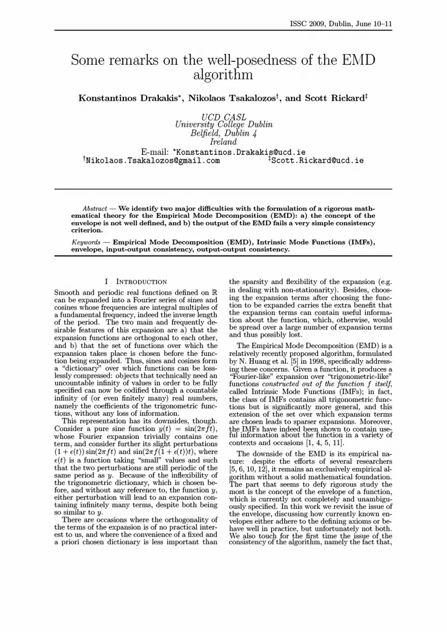
We set the parameters stop= [10-7,10-7,10-7] and maxiterations= 105; these parameters force the algorithm to work with an accuracy way be­yond the default level. Furthermore, we sample the function using a sampling interval of 10-4: this sampling rate is much higher than the Nyquist rate, hence the mismatch between the sampled and the actual extrema, which could potentially degrade the operation of the algorithm, should be negligible. Running the EMD on I yields six IMFs, the last four of which we recognize as "artifacts" (only because we know the function in closed form, though, otherwise we could not possibly do that). Subsequently, we repeatedly summed the first two IMFs of each output (which we recognize as the IMFs "that should be in the expansion" ) and we ran EMD on this sum, performing this procedure eight times: we systematically obtained eight or nine IMFs each time, but, at the last iteration, the energy of the artifacts was between 1012 and 1015 times smaller than the energy of the main two IMFs, so we may ignore the "artifacts" of this last iteration and consider that the iterated IMD has converged, for all practical purposes.

Figure 1 shows the results of this expansion. It appears that the iterative refinement of the two

0.8

0.6

0.4

0.2

-0.2

-0.4

-0.6

-0.8

-1

1.5

0.5

-0.5

-1

-1.5 o

W

�

_f, - OriginallMF - Last iteration IMF

-f2 - OriginallMF - Last iteration IMF

0.2 0.4 0.6 0.8

Fig. 1: The two main IMFs resulting from applying high-accuracy EMD on h + 12, along with the IMFs

resulting from repeated application of the EMD on the sum of the two main IMFs on each output. The

approximation is very good, except for a small but noticeable deviation at the edges of h.

main IMFs did not lead to any substantial change, so OO-consistency is essentially satisfied here. Re­garding IO-consistency, however, there seem to be small but noticeable deviations of the recovered IMFs from the original ones, in particular for the low frequency IMF fl towards the edges, which cannot readily be attributed to numerical errors. The most likely source of this error seems to be edge effects due to the construction of the en­velopes through interpolation. This stresses the importance of investigating appropriate edge con­ditions for the construction of the envelopes.

Using the default stopping parameters stop= [0.050.50.05] , performing EMD on f yields five IMFs. Summing the first two and performing EMD on this sum yields the same two IMFs, so in this case OO-consistency is fully satisfied. The recovered IMFs, however, are very far from the original ones, as Figure 2 shows (frequency is accu­rately captured but not amplitude), especially the low frequency one, so IO-consistency is not satis­fied.

Consider now the function f(t) = sin(201ft) + 1.3 sin(301ft) +

1.1 sin( 401ft) + 0.9 sin (501ft ), t E [0, 1] , (11) which is the sum of the four trigonometric func­tions h, 12,

13(t) = 1.1 sin(401ft),

and f4(t) = 0.9 sin(501ft). (12) We now set stop= [10-6, 10-6, 10-6] ; this param­eters also forces the algorithm to work with an ac­curacy way beyond the default level. Running the

1

1\ Ii 0.8

I-f, 1/'1 -IMF 1/\ /(\ f\ If\

11\1 /\ If\ f\

0.6

0.4

0.2

-0.2 v IV v IV IV v

-0.4

-0.6

-0.8

1

2.5rr=====;-�-�--�--�--1 2 -- f2

--IMF 1.5

0.5

-0.5

-1

-1.5

-2

-2.5'-----�--�--�--�-----' o 0.2 0.4 0.6 0.8

Fig. 2: The two main IMFs resulting from applying low-accuracy EMD on h + h. The IMFs resulting from repeated application of the EMD on the sum of the two main IMFs are identical to the two main original IMFs and not shown here. Amplitude approximation is poor, though frequency is accurately captured in both cases.

EMD on f yields eight IMFs, the last four of which we consider to be "artifacts" , while the first four correspond reasonably well to h, 12, 13, and f4' to an extent that IO-consistency in this specific case may be justified with an appropriately high toler­ance (see Figure 3). We subsequently apply the EMD again to the sums of h, f4' and IMF 5 of the output, and also of 12, f4' and IMF5 (IMF5 is con­sidered an artifact). Figure 3 shows that, although OO-consistency can be marginally justified in the case of h, though there are noticeable deviations, especially near the end points, it is certainly not satisfied in the case of IMF5.

The loosely related problem of the classification of functions expandable into (at most) an arbi­trary but fixed number of IMFs has been raised and studied in [13] . The authors considered weak IMFs instead, which they themselves defined and studied in [12] (see also Section b)), and concluded that any sufficiently smooth function is the sum of at most two weak IMFs.

V CONCLUSION A mathematical study of an ob­ject/problem/algorithm is only possible when this object/problem/algorithm is well-posed, and we claim that the EMD, as is currently formulated, is not well posed. Its main weakness appears to be the specification of the envelope of a function, which is not only ambiguous, but necessitates a significant deviation from the currently proposed theoretical axiomatization in order to yield good results in practice, and, in

1.5

fI � fI � 1

0.5 \ \ -I,

\ -IMF

1\ -IMF rec.

-0.5

1 V � V V � -1.5

Fig. 3: (Left) h shown along with its corresponding IMF and the reconstructed IMF out of the sum h + /4 + 1MF5 (Right) 1MF5 along with its two reconstructions out of the

sums h + /4 + 1MF5 and /2 + /4 + 1MF5.

turn, makes the concept of the IMF also ill-posed. Even if we define IMFs empirically as outputs

of the EMD, consistency issues arise: the sum of functions individually recognized as IMFs by the EMD does not decompose into the same set of IMFs (IO-consistency), and, furthermore, par­tial sums of these resulting IMFs do not decom­pose into the same set of summed IMFs (00-consistency). The cause for this inconsistency is most likely end effects resulting from the subop­timal definition of the envelopes near the end­points of the observation interval. We feel that the present situation detracts much of the value of the EMD, and that future efforts should concentrate on improving the axiomatization of the envelope and on producing a version of the EMD algorithm that is at least OO-consistent.

But do we have the right to expect that an a posteriori expansion rule such as the EMD must satisfy a consistency criterion formulated through our experience with a priori expansion rules? If, instead, we assume that the IMFs are supposed to interact, so that the very fact that we obtain a certain IMF in the expansion depends heavily on the fact that the input function was the sum of the specific set of IMFs obtained, then what does con­sistency mean in the context of EMD? What is the corresponding appropriate consistency criterion, if any, and how should the output be interpreted?

REFERENCES [1] K. Drakakis. "Empirical Mode Decomposition

of financial data." International Mathemat­ical Forum, Volume 3, Issue 25, 2008, pp. 1191-1202.

[2] R Deering, J.F. Kaiser. "The use Of a mask­ing signal to improve Empirical Mode Decom­position." ICASSP 2005, Volume IV, pp. 485-488.

[3] P. Flandrin. Matlab implementation of the EMD found at http://perso.ens­lyon.fr / patrick.flandrin/ emd.html.

[4] K. Guhathakurta, I. Mukherjee, A. Chowd­hury. "Empirical Mode Decomposition anal­ysis of two different financial time-series and their comparison." Chaos, Solitons and Frac­tals, Volume 37, 2008, pp. 1214-1227.

[5] N.E. Huang, Z. Shen, S.R Long, M.C. Wu, E.H. Shih, Q. Zheng, C.C. Tung, H.H. Liu. "The Empirical Mode Decomposition Method and the Hilbert Spectrum for Non-stationary Time Series Analysis." Proceedings of the Royal Society of London, Series A, Volume 454, 1998, pp. 903-995.

[6] N.E. Huang, M.C. Wu, S.R Long, S.S.P. Shen, W. Qu, P. Gloersen, K.L. Fan. "A confi­dence limit for the Empirical Mode Decompo­sition and Hilbert spectral analysis." Proceed­ings of the Royal Society of London, Series A, Volume 459, 2003, pp. 2317-2345.

[7] Y. Kopsinis, S. McLaughlin. "Investigation and Performance Enhancement of the Empir­ical Mode Decomposition Method Based on a Heuristic Search Optimization Approach." IEEE Transactions On Signal Processing, Vol­ume 56, Issue 1, January 2008, pp. 1-13.

[8] M.C. Peel, T.A. McMahon, G.G.S. Pegram. "Assessing the performance of rational spline­based Empirical Mode Decomposition using a global annual precipitation dataset." Proceed­ings of the Royal Society of London, Series A, April 2009 (online publication).

[9] G.G.S Pegram, M.C Peel, T.A McMahon. "Empirical Mode Decomposition using ratio­nal splines: an application to rainfall time se­ries." Proceedings of the Royal Society of Lon­don, Series A, Volume 464, 2008, pp. 1483-1501.

[10] G. Rilling, P. Flandrin. "One or two frequen­cies? The Empirical Mode Decomposition an­swers." IEEE Transactions on Signal Process­ing, Volume 56, Issue 1, January 2008, pp. 85-95.

[11] G. Rilling, P. Flandrin and P. Gongalves. "On Empirical Mode Decomposition and its algo­rithms." IEEE-EURASIP Workshop on Non­linear Signal and Image Processing, NSIP-03, Grado (I), June 2003.

[12] RC. Sharpley, V. Vatchev. "Analysis of the Intrinsic Mode Functions." Constructive Ap­proximation, Volume 24, Issue 1, 2006, pp. 17-47.

[13] V. Vatchev, RC. Sharpley. "Decomposition of functions into pairs of Intrinsic Mode Func­tions." Proceedings of the Royal Society of London, Series A, Volume 464, 2008, pp. 2265-2280.

[14] S. Wang. "Simple proofs of the Bedrosian equality for the Hilbert transform." Science in China Series A: Mathematics, Volume 52, Issue 3, March 2009, pp. 507-510.