Tectonophysics 623 (2014) 23–38

Contents lists available at ScienceDirect

Tectonophysics

j ourna l homepage: www.e lsev ie r .com/ locate / tecto

Source parameters of the December 2011–January 2012 earthquakesequence in Southern Carpathians, Romania

M. Radulian a,b,⁎, E. Popescu a, F. Borleanu a, M. Diaconescu a

a National Institute for Earth Physics, Măgurele, 12 Călugăreni str., 077125 Ilfov, Romaniab Academy of Romanian Scientists, 54 Splaiul Independentei, RO-050094 Bucharest, Romania

⁎ Corresponding author at: National Institute for Earth Pstr., 077125 Ilfov, Romania.

E-mail address: mircea@infp.ro (M. Radulian).

http://dx.doi.org/10.1016/j.tecto.2014.03.0140040-1951/© 2014 Elsevier B.V. All rights reserved.

a b s t r a c t

a r t i c l e i n f o

Article history:Received 28 June 2013Received in revised form 14 March 2014Accepted 15 March 2014Available online 22 March 2014

Keywords:Earthquake sequenceSource parametersEmpirical Green's functionSpectral ratiosScaling relationships

The seismicity at the contact between the Getic Depression and the South Carpathians is part of the overall seis-micity characterizing the contact of the Moesian Platform and the South Carpathians orogen. The December2011–January 2012 earthquake sequence that occurred close to Tg-Jiu city provides the best data set for the seis-mic activity in the region. The seismic source parameters are estimated for 15 events of the sequence using theempirical Green's function and spectral ratio techniques.We selected 3main events and 12 associated collocatedsmall events as empirical Green's functions to calculate the spectral ratios and determine the relative source timefunctions. Estimates of the source duration and corner frequency imply stress drop values in the range of 6–112MPa. Relative small radius of the source and high stress drops suggest an intraplate type behaviour. The scalingrelationships investigated comply well with similar relationships in other regions in the world and in otherseismogenic areas in the South Carpathians region.

© 2014 Elsevier B.V. All rights reserved.

1. Introduction

Seismicity in Romania follows generally the line of Carpathians(Fig. 1) with a sharp concentration at the mountain arc bend in theVrancea region. Some seismicity clusters are recorded in the extra-Carpathian area as well, especially in front of the CarpathiansArc bend (foredeep region) and in the western part of the country(see Radulian et al., 2000, for more details). Weak to moderateearthquakes are recorded from time to time along the SouthernCarpathians, between the two sharp curvatures, one to the east atthe contact with the Eastern Carpathians branch, the other to thewest, where orogen turns southward. The largest events were re-corded in the Făgăraş–Câmpulung seismogenic area (Mw ~ 6.5). Fre-quently the earthquakes are generated in sequences (Enescu et al.,1996; Popescu, 2000; Popescu and Radulian, 2001; Popescu et al.,2011, 2012). Such a sequence was recently recorded close to Tg-Jiucity. The aim of the present paper is to investigate the characteristicsof this earthquake sequence.

The sequence started on December 30, 2011, lasting until January5, 2012. Based on the real-time seismic network of the National In-stitute for Earth Physics (NIEP), 40 events of the sequence wereidentified and located nearby Tg-Jiu–Tg-Carbunesti (Table 1). The

hysics, Măgurele, 12 Călugăreni

largest shock (MD = 4.5) occurred on January 01, 2012, at23:57:19 UTC. It was preceded by 7 foreshocks and followed by 32aftershocks. Other four events have duration magnitude (MD)above 3.5. According to the ROMPLUS catalogue (Oncescu et al.,1999, continuously updated), the hypocentre coordinates of thelargest shock were 45.04°N — latitude, 23.56°E — longitude, and14 km — depth.

Previous seismicity in the same region is limited to 34 earth-quakes which have been recorded since 20th century (Oncescuet al., 1999, with updates). They are only small-to-moderate sizeevents (Mw magnitude between 2.5 and 4.5), with only two eventsof magnitude Mw above 4 (9 July 1912 at 21:46, Mw = 4.5 and 4May 1963 at 16:48, Mw = 4.5). All the events recorded after 2000are of small magnitude (below 3). From this point of view, the recentsequence represents a relative enhancement in seismicity for thestudy area.

The earthquakes are located nearby the contact between GeticDepression and the Carpathians orogen. The Getic Depression liesin front of the Southern Carpathians from Târgu River in the east, tothe Danube valley to the west. It is bordered to the south bythe Pericarpathian Fault, at the contact with Moesian Platform. TheGetic Depression is the most internal and deformed part of theforedeep in the South Carpathians foreland. It is buried below thepost tectonic cover of the Dacic basin and thrust over the Moesianforeland (Schmid et al., 2008). Therefore, the basement of the GeticDepression is of Moesian type (Matenco et al., 2010).

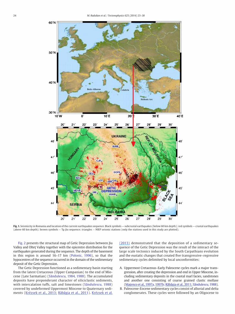
Fig. 1. Seismicity in Romania and location of the current earthquakes sequence. Black symbols— subcrustal earthquakes (below 60 km depth); red symbols— crustal earthquakes(above 60 km depth); brown symbols — Tg-Jiu sequence; triangles — NIEP seismic stations (only the stations used in this study are plotted).

24 M. Radulian et al. / Tectonophysics 623 (2014) 23–38

Fig. 2 presents the structural map of Getic Depression between JiuValley and Olteţ Valley together with the epicentre distribution for theearthquakes generated during the sequence. The depth of the basementin this region is around 16–17 km (Polonic, 1996), so that thehypocentres of the sequence occurred in the domain of the sedimentarydeposit of the Getic Depression.

The Getic Depression functioned as a sedimentary basin startingfrom the latest Cretaceous (Upper Campanian) to the end of Mio-cene (Late Sarmatian) (Săndulescu, 1984, 1988). The accumulateddeposits have preponderant character of siliciclastic sediments,with intercalation tuffs, salt and limestones (Săndulescu, 1988)covered by undeformed Uppermost Miocene to Quaternary sedi-ments (Krézsek et al., 2013; Răbăgia et al., 2011). Krézsek et al.

(2013) demonstrated that the deposition of a sedimentary se-quence of the Getic Depression was the result of the interact of thelarge scale tectonics induced by the South Carpathians evolutionand the eustatic changes that created five transgressive–regressivesedimentary cycles delimited by local unconformities:

A. Uppermost Cretaceous–Early Paleocene cycles mark a major trans-gression, after creating the depression and end in Upper Miocene, in-cluding sedimentary deposits in the coastal marl facies, sandstonesand another one consisting of coarse grained clastic mollase(Maţenco et al., 1997a, 1997b; Răbăgia et al., 2011; Săndulescu, 1988).

B. Paleocene-Eocene sedimentary cycles consist of alluvial and deltaconglomerates. These cycles were followed by an Oligocene to

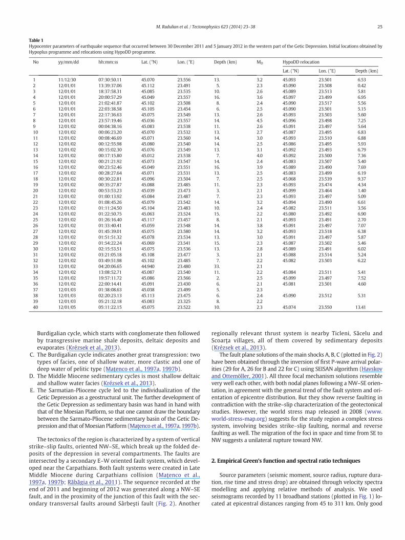
Table 1Hypocenter parameters of earthquake sequence that occurred between 30 December 2011 and 5 January 2012 in the western part of the Getic Depression. Initial locations obtained byHypoplus programme and relocations using HypoDD programme.

No yy/mm/dd hh:mm:ss Lat. (°N) Lon. (°E) Depth (km) MD HypoDD relocation

Lat. (°N) Lon. (°E) Depth (km)

1 11/12/30 07:30:50.11 45.070 23.556 13. 3.2 45.093 23.501 6.532 12/01/01 13:39:37.06 45.112 23.491 5. 2.3 45.090 23.508 0.423 12/01/01 18:37:58.31 45.085 23.535 10. 2.6 45.089 23.513 5.814 12/01/01 20:00:57.29 45.049 23.557 16. 3.6 45.097 23.499 6.955 12/01/01 21:02:41.87 45.102 23.508 8. 2.4 45.090 23.517 5.566 12/01/01 22:03:38.58 45.105 23.454 6. 2.5 45.090 23.501 5.157 12/01/01 22:17:36.63 45.075 23.549 13. 2.6 45.093 23.503 5.608 12/01/01 23:57:19.46 45.036 23.557 14. 4.5 45.096 23.498 7.259 12/01/02 00:04:38.16 45.083 23.538 11. 2.6 45.091 23.497 5.6410 12/01/02 00:06:23.20 45.070 23.532 13. 2.7 45.087 23.495 6.8311 12/01/02 00:08:46.69 45.071 23.560 14. 3.0 45.093 23.510 6.8812 12/01/02 00:12:55.98 45.080 23.540 14. 2.5 45.086 23.495 5.9313 12/01/02 00:15:02.30 45.076 23.549 13. 3.1 45.092 23.493 6.7914 12/01/02 00:17:15.80 45.012 23.538 7. 4.0 45.092 23.500 7.3615 12/01/02 00:21:21.92 45.073 23.547 14. 2.4 45.083 23.507 5.4016 12/01/02 00:23:52.46 45.049 23.551 16. 3.9 45.089 23.490 7.6917 12/01/02 00:28:27.64 45.071 23.531 13. 2.5 45.083 23.499 6.1918 12/01/02 00:30:22.81 45.096 23.504 7. 2.5 45.068 23.539 9.3719 12/01/02 00:35:27.87 45.088 23.485 11. 2.3 45.093 23.474 4.3420 12/01/02 00:53:53.23 45.039 23.473 3. 2.1 45.099 23.464 1.4021 12/01/02 01:00:13.92 45.084 23.487 7. 2.3 45.093 23.497 5.0922 12/01/02 01:08:45.26 45.079 23.542 14. 3.2 45.094 23.490 6.6123 12/01/02 01:11:24.50 45.104 23.483 10. 2.4 45.082 23.511 3.5624 12/01/02 01:22:50.75 45.063 23.524 15. 2.2 45.080 23.492 6.9025 12/01/02 01:26:16.40 45.117 23.457 8. 2.1 45.093 23.491 2.7026 12/01/02 01:33:40.41 45.059 23.548 14. 3.8 45.091 23.497 7.0727 12/01/02 01:45:39.01 45.075 23.580 14. 3.2 45.093 23.518 6.3828 12/01/02 01:51:51.32 45.078 23.534 13. 3.0 45.091 23.497 5.8729 12/01/02 01:54:22.24 45.069 23.541 15. 2.3 45.087 23.502 5.4630 12/01/02 02:15:53.51 45.075 23.536 13. 2.8 45.089 23.491 6.0231 12/01/02 03:21:05.18 45.108 23.477 3. 2.1 45.088 23.514 5.2432 12/01/02 03:49:51.98 45.102 23.485 7. 2.2 45.082 23.503 6.2233 12/01/02 04:20:06.65 44.940 23.480 33. 2.134 12/01/02 13:08:52.71 45.087 23.540 11. 2.2 45.084 23.511 5.4135 12/01/02 19:57:11.72 45.086 23.566 2. 2.5 45.099 23.497 7.5236 12/01/02 22:00:14.41 45.091 23.430 6. 2.1 45.081 23.501 4.6037 12/01/03 01:38:08.63 45.038 23.499 5. 2.338 12/01/03 02:20:23.13 45.113 23.475 6. 2.4 45.090 23.512 5.3139 12/01/03 05:21:32.18 45.083 23.325 8. 2.240 12/01/05 05:11:22.15 45.075 23.522 10. 2.3 45.074 23.550 13.41

25M. Radulian et al. / Tectonophysics 623 (2014) 23–38

Burdigalian cycle, which starts with conglomerate then followedby transgressive marine shale deposits, deltaic deposits andevaporates (Krézsek et al., 2013).

C. The Burdigalian cycle indicates another great transgression: twotypes of facies, one of shallow water, more clastic and one ofdeep water of pelitic type (Maţenco et al., 1997a, 1997b).

D. The Middle Miocene sedimentary cycles is most shallow deltaicand shallow water facies (Krézsek et al., 2013).

E. The Sarmatian-Pliocene cycle led to the individualization of theGetic Depression as a geostructural unit. The further development ofthe Getic Depression as sedimentary basin was hand in hand withthat of the Moesian Platform, so that one cannot draw the boundarybetween the Sarmato-Pliocene sedimentary basin of the Getic De-pression and that ofMoesian Platform (Maţenco et al., 1997a, 1997b).

The tectonics of the region is characterized by a system of verticalstrike–slip faults, oriented NW–SE, which break up the folded de-posits of the depression in several compartments. The faults areintersected by a secondary E–W oriented fault system, which devel-oped near the Carpathians. Both fault systems were created in LateMiddle Miocene during Carpathians collision (Maţenco et al.,1997a, 1997b; Răbăgia et al., 2011). The sequence recorded at theend of 2011 and beginning of 2012 was generated along a NW–SEfault, and in the proximity of the junction of this fault with the sec-ondary transversal faults around Sârbeşti fault (Fig. 2). Another

regionally relevant thrust system is nearby Ticleni, Săcelu andScoarţa villages, all of them covered by sedimentary deposits(Krézsek et al., 2013).

The fault plane solutions of themain shocks A, B, C (plotted in Fig. 2)have been obtained through the inversion of first P-wave arrival polar-ities (29 for A, 26 for B and 22 for C) using SEISAN algorithm (Havskovand Ottemöller, 2001). All three focal mechanism solutions resemblevery well each other, with both nodal planes following a NW–SE orien-tation, in agreement with the general trend of the fault system and ori-entation of epicentre distribution. But they show reverse faulting incontradiction with the strike–slip characterization of the geotectonicalstudies. However, the world stress map released in 2008 (www.world-stress-map.org) suggests for the study region a complex stresssystem, involving besides strike–slip faulting, normal and reversefaulting as well. The migration of the foci in space and time from SE toNW suggests a unilateral rupture toward NW.

2. Empirical Green's function and spectral ratio techniques

Source parameters (seismic moment, source radius, rupture dura-tion, rise time and stress drop) are obtained through velocity spectramodelling and applying relative methods of analysis. We usedseismograms recorded by 11 broadband stations (plotted in Fig. 1) lo-cated at epicentral distances ranging from 45 to 311 km. Only good

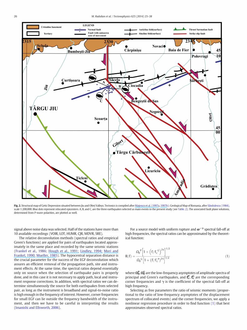
Fig. 2. StructuralmapofGeticDepression situatedbetween Jiu andOlteţValleys. Tectonics is compiled afterMaţenco et al. (1997a, 1997b);GeologicalMapof Romania, after Săndulescu (1984),scale 1:200,000. Blue dots represent relocated epicenters. A, B, and C, are the three earthquakes selected asmain events in the present study (see Table. 2). The associated fault plane solutions,determined from P-wave polarities, are plotted as well.

26 M. Radulian et al. / Tectonophysics 623 (2014) 23–38

signal abovenoise datawas selected.Half of the stationshavemore than10 available recordings (VOIR, LOT, HUMR, CJR, MDVR, SRE).

The relative deconvolution methods (spectral ratios and empiricalGreen's functions) are applied for pairs of earthquakes located approx-imately in the same place and recorded by the same seismic stations(Frankel et al., 1986; Hough et al., 1991; Lindley, 1994; Mori andFrankel, 1990; Mueller, 1985). The hypocentral separation distance isthe crucial parameter for the success of the EGF deconvolution whichassures an efficient removal of the propagation path, site and instru-ment effects. At the same time, the spectral ratios depend essentiallyonly on source when the selection of earthquake pairs is properlydone, and in this case it is not necessary to apply path, local and instru-ment response corrections. In addition, with spectral ratios we can de-termine simultaneously the source for both earthquakes from selectedpair, as long as the instrument is broadband and signal-to-noise ratiois high enough in the frequency of interest. However, corner frequenciesfor small EGF can lie outside the frequency bandwidth of the instru-ment, and then we have to be careful in interpreting the results(Imanishi and Ellsworth, 2006).

For a source model with uniform rupture and ω−γ spectral fall-off athigh frequencies, the spectral ratios can be approximated by the theoret-ical function:

R fð Þ ¼Ω0

P 1þ f= fcG

� �2γ� �1=2

Ω0G 1þ f= f c

P� �2γh i1=2 ð1Þ

whereΩ0P,Ω0

G are the low-frequency asymptotes of amplitude spectra ofprincipal and Green's earthquakes, and fcP, fcG are the correspondingcorner frequencies and γ is the coefficient of the spectral fall-off athigh frequency.

Selecting as free parameters the ratio of seismic moments (propor-tional to the ratio of low-frequency asymptotes of the displacementspectrum of collocated events) and the corner frequencies, we apply anonlinear regression procedure in order to find function (1) that bestapproximates observed spectral ratios.

27M. Radulian et al. / Tectonophysics 623 (2014) 23–38

The size of the rupture area is directly related to the corner frequency(Madariaga, 1976):

r ¼ kvS= f c ð2Þr representing the equivalent radius of the source. k is a constant k=0.32for P waves and k= 0.21 for S waves, fc is the corner frequency and vS isthe S-wave velocity in the focus. With relationship (2) we determine thesource radius from corner frequencies (rGrs — radius of Green function

-2E+4-2E+4-1E+4-5E+3

05E+31E+42E+42E+4

0 10 20

-1E+3

-5E+2

0

5E+2

1E+3

2E+3

0 10 20

-2E+4-2E+4-1E+4-5E+3

05E+31E+42E+42E+4

0 10 20

-2E+3-2E+3-1E+3-5E+2

05E+21E+32E+3

0 10 20

E

E

-1E+4

-8E+3

-4E+3

0

4E+3

8E+3

1E+4

0 10 20

-2E+3

-1E+3

-5E+2

0

5E+2

1E+3

ampl

itude

(co

unts

/s)

0 10 20

N

N

BZS

Z

Z

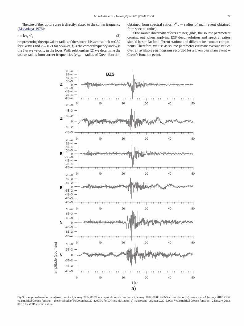
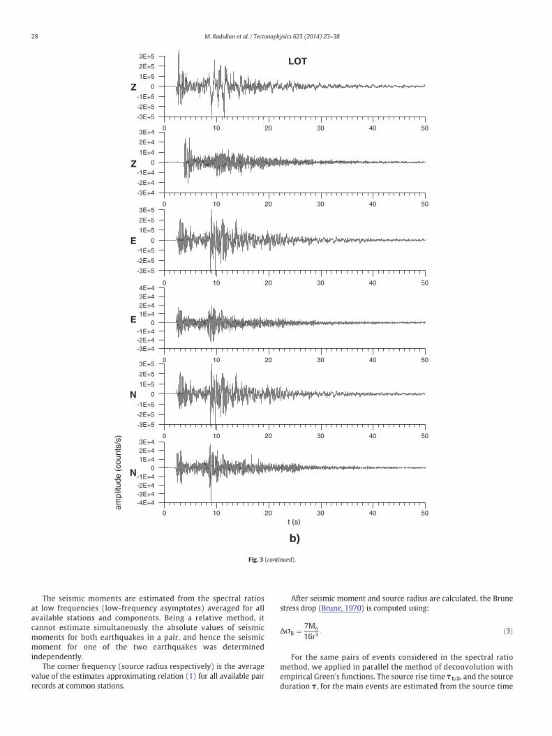
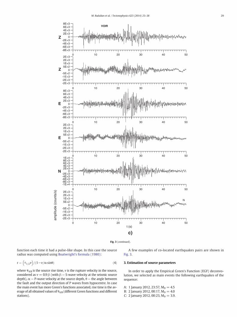
Fig. 3.Examples ofwaveforms: a)main event – 2 January, 2012, 00:23 vs. empirical Green’s funcvs. empirical Green’s function – the foreshock of 30 December, 2011, 07:30 for LOT seismic stati00:15 for VOIR seismic station.

obtained from spectral ratios, rPrs — radius of main event obtainedfrom spectral ratios).

If the source directivity effects are negligible, the source parameterscoming out when applying EGF deconvolution and spectral ratiosshould be similar for different stations and different instrument compo-nents. Therefore, we use as source parameter estimate average valuesover all available seismograms recorded for a given pair main event —Green's function event.

30 40 50

30 40 50

30 40 50

30 40 50

30 40 50

30 40 50

t (s)

a)

tion – 2 January, 2012, 00:08 for BZS seismic station; b)main event – 1 January, 2012, 23:57on; c)main event – 2 January, 2012, 00:17 vs. empirical Green’s function – 2 January, 2012,

-3E+5

-2E+5

-1E+5

0

1E+5

2E+5

3E+5

0 10 20 30 40 50

-3E+4

-2E+4

-1E+4

0

1E+4

2E+4

3E+4

0 10 20 30 40 50

-3E+5

-2E+5

-1E+5

0

1E+5

2E+5

3E+5

0 10 20 30 40 50

-3E+4-2E+4-1E+4

01E+42E+43E+44E+4

0 10 20 30 40 50

E

E

-3E+5

-2E+5

-1E+5

0

1E+5

2E+5

3E+5

0 10 20 30 40 50

-4E+4-3E+4-2E+4-1E+4

01E+42E+43E+4

ampl

itude

(co

unts

/s)

0 10 20 30 40 50t (s)

N

N

LOT

Z

Z

b)

Fig. 3 (continued).

28 M. Radulian et al. / Tectonophysics 623 (2014) 23–38

The seismic moments are estimated from the spectral ratiosat low frequencies (low-frequency asymptotes) averaged for allavailable stations and components. Being a relative method, itcannot estimate simultaneously the absolute values of seismicmoments for both earthquakes in a pair, and hence the seismicmoment for one of the two earthquakes was determinedindependently.

The corner frequency (source radius respectively) is the averagevalue of the estimates approximating relation (1) for all available pairrecords at common stations.

After seismic moment and source radius are calculated, the Brunestress drop (Brune, 1970) is computed using:

ΔσB ¼ 7Mo

16r3: ð3Þ

For the same pairs of events considered in the spectral ratiomethod, we applied in parallel the method of deconvolution withempirical Green's functions. The source rise time τ1/2, and the sourceduration τ, for the main events are estimated from the source time

-8E+3-6E+3-4E+3-2E+3

02E+34E+36E+38E+3

0 10 20 30 40 50

-2E+3-2E+3-1E+3-5E+2

05E+21E+32E+32E+3

0 10 20 30 40 50

-8E+3-6E+3-4E+3-2E+3

02E+34E+36E+38E+3

0 10 20 30 40 50

-2E+3-2E+3-1E+3-5E+2

05E+21E+32E+32E+3

0 10 20 30 40 50

E

E

-1E+4-8E+3-6E+3-4E+3-2E+3

02E+34E+36E+38E+31E+4

0 10 20 30 40 50

-2E+3-2E+3-1E+3-5E+2

05E+21E+32E+32E+3

ampl

itude

(co

unts

/s)

0 10 20 30 40 50t (s)

N

N

VOIR

Z

Z

c)

Fig. 3 (continued).

29M. Radulian et al. / Tectonophysics 623 (2014) 23–38

function each time it had a pulse-like shape. In this case the sourceradius was computed using Boatwright's formula (1980):

r ¼ τ1=2v� �

= 1−v=α sinθð Þ ð4Þ

where τ1/2 is the source rise time, v is the rupture velocity in the source,considered as v = 0.9 β (with β — S-wave velocity at the seismic sourcedepth), α — P-wave velocity at the source depth, θ — the angle betweenthe fault and the output direction of P waves from hypocentre. In casethemain event has more Green's functions associated, rise time is the av-erage of all obtained values ofτ1/2 (different Green functions anddifferentstations).

A few examples of co-located earthquakes pairs are shown inFig. 3.

3. Estimation of source parameters

In order to apply the Empirical Green's Function (EGF) deconvo-lution, we selected as main events the following earthquakes of thesequence:

A: 1 January 2012, 23:57, MD = 4.5B: 2 January 2012, 00:17, MD = 4.0C: 2 January 2012, 00:23, MD = 3.9.

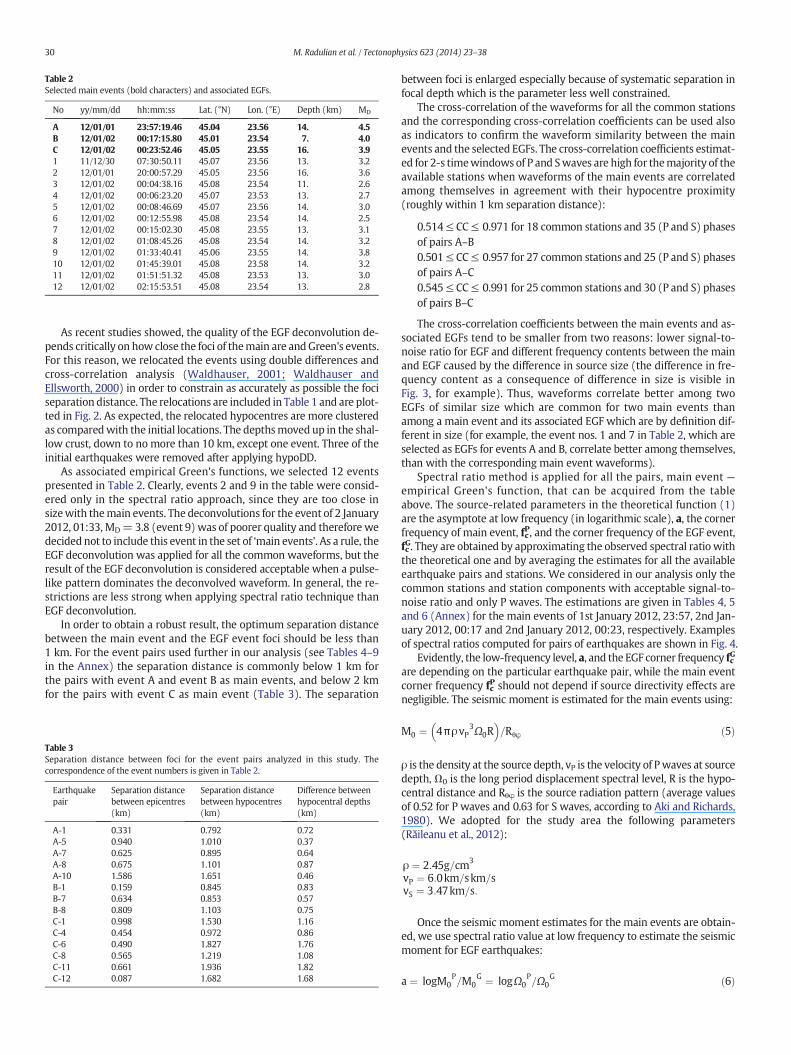
Table 2Selected main events (bold characters) and associated EGFs.

No yy/mm/dd hh:mm:ss Lat. (°N) Lon. (°E) Depth (km) MD

A 12/01/01 23:57:19.46 45.04 23.56 14. 4.5B 12/01/02 00:17:15.80 45.01 23.54 7. 4.0C 12/01/02 00:23:52.46 45.05 23.55 16. 3.91 11/12/30 07:30:50.11 45.07 23.56 13. 3.22 12/01/01 20:00:57.29 45.05 23.56 16. 3.63 12/01/02 00:04:38.16 45.08 23.54 11. 2.64 12/01/02 00:06:23.20 45.07 23.53 13. 2.75 12/01/02 00:08:46.69 45.07 23.56 14. 3.06 12/01/02 00:12:55.98 45.08 23.54 14. 2.57 12/01/02 00:15:02.30 45.08 23.55 13. 3.18 12/01/02 01:08:45.26 45.08 23.54 14. 3.29 12/01/02 01:33:40.41 45.06 23.55 14. 3.810 12/01/02 01:45:39.01 45.08 23.58 14. 3.211 12/01/02 01:51:51.32 45.08 23.53 13. 3.012 12/01/02 02:15:53.51 45.08 23.54 13. 2.8

30 M. Radulian et al. / Tectonophysics 623 (2014) 23–38

As recent studies showed, the quality of the EGF deconvolution de-pends critically on how close the foci of themain are andGreen's events.For this reason, we relocated the events using double differences andcross-correlation analysis (Waldhauser, 2001; Waldhauser andEllsworth, 2000) in order to constrain as accurately as possible the fociseparation distance. The relocations are included in Table 1 and are plot-ted in Fig. 2. As expected, the relocated hypocentres are more clusteredas comparedwith the initial locations. The depthsmoved up in the shal-low crust, down to no more than 10 km, except one event. Three of theinitial earthquakes were removed after applying hypoDD.

As associated empirical Green's functions, we selected 12 eventspresented in Table 2. Clearly, events 2 and 9 in the table were consid-ered only in the spectral ratio approach, since they are too close insizewith themain events. The deconvolutions for the event of 2 January2012, 01:33,MD=3.8 (event 9) was of poorer quality and therefore wedecided not to include this event in the set of ‘main events’. As a rule, theEGF deconvolution was applied for all the common waveforms, but theresult of the EGF deconvolution is considered acceptable when a pulse-like pattern dominates the deconvolved waveform. In general, the re-strictions are less strong when applying spectral ratio technique thanEGF deconvolution.

In order to obtain a robust result, the optimum separation distancebetween the main event and the EGF event foci should be less than1 km. For the event pairs used further in our analysis (see Tables 4–9in the Annex) the separation distance is commonly below 1 km forthe pairs with event A and event B as main events, and below 2 kmfor the pairs with event C as main event (Table 3). The separation

Table 3Separation distance between foci for the event pairs analyzed in this study. Thecorrespondence of the event numbers is given in Table 2.

Earthquakepair

Separation distancebetween epicentres(km)

Separation distancebetween hypocentres(km)

Difference betweenhypocentral depths(km)

A-1 0.331 0.792 0.72A-5 0.940 1.010 0.37A-7 0.625 0.895 0.64A-8 0.675 1.101 0.87A-10 1.586 1.651 0.46B-1 0.159 0.845 0.83B-7 0.634 0.853 0.57B-8 0.809 1.103 0.75C-1 0.998 1.530 1.16C-4 0.454 0.972 0.86C-6 0.490 1.827 1.76C-8 0.565 1.219 1.08C-11 0.661 1.936 1.82C-12 0.087 1.682 1.68

between foci is enlarged especially because of systematic separation infocal depth which is the parameter less well constrained.

The cross-correlation of the waveforms for all the common stationsand the corresponding cross-correlation coefficients can be used alsoas indicators to confirm the waveform similarity between the mainevents and the selected EGFs. The cross-correlation coefficients estimat-ed for 2-s timewindows of P and Swaves are high for themajority of theavailable stations when waveforms of the main events are correlatedamong themselves in agreement with their hypocentre proximity(roughly within 1 km separation distance):

0.514≤ CC≤ 0.971 for 18 common stations and 35 (P and S) phasesof pairs A–B0.501≤ CC≤ 0.957 for 27 common stations and 25 (P and S) phasesof pairs A–C0.545≤ CC≤ 0.991 for 25 common stations and 30 (P and S) phasesof pairs B–C

The cross-correlation coefficients between the main events and as-sociated EGFs tend to be smaller from two reasons: lower signal-to-noise ratio for EGF and different frequency contents between the mainand EGF caused by the difference in source size (the difference in fre-quency content as a consequence of difference in size is visible inFig. 3, for example). Thus, waveforms correlate better among twoEGFs of similar size which are common for two main events thanamong a main event and its associated EGF which are by definition dif-ferent in size (for example, the event nos. 1 and 7 in Table 2, which areselected as EGFs for events A and B, correlate better among themselves,than with the corresponding main event waveforms).

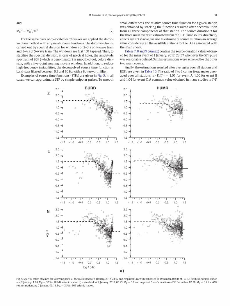
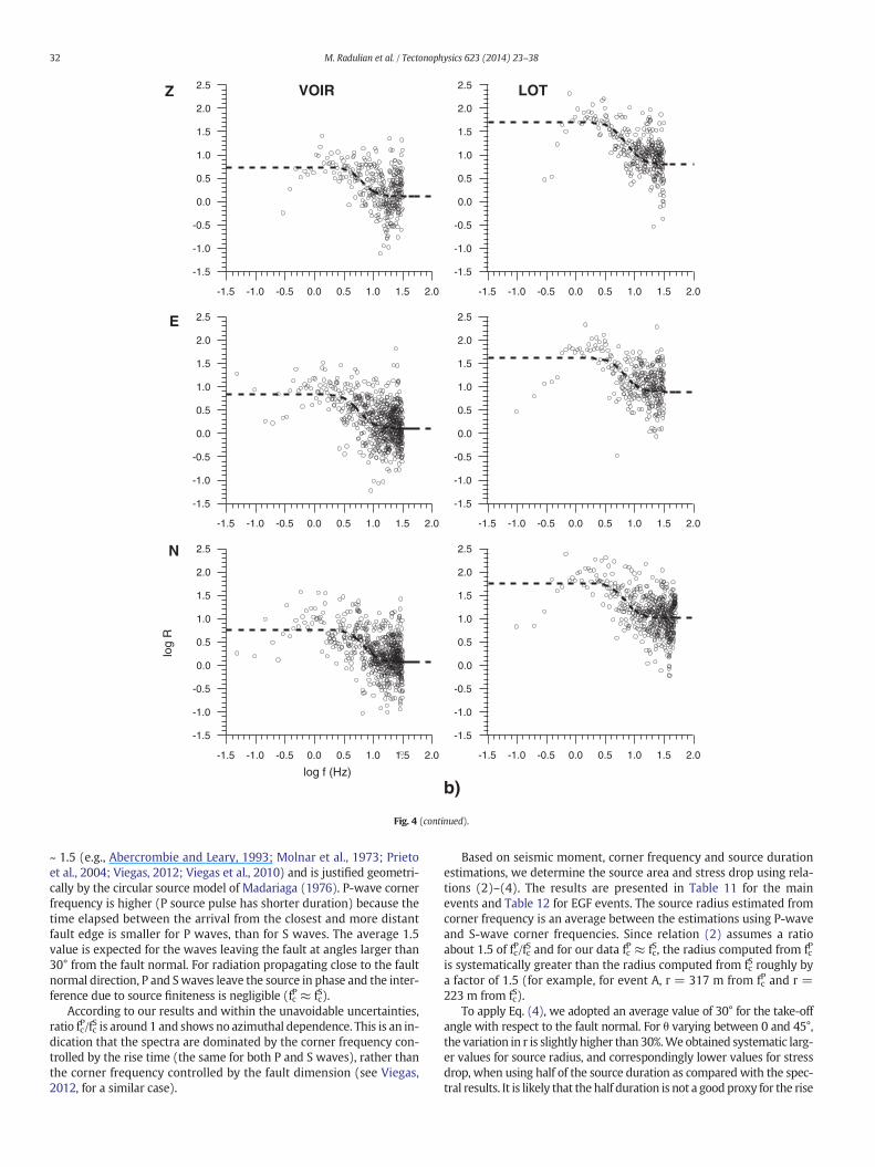
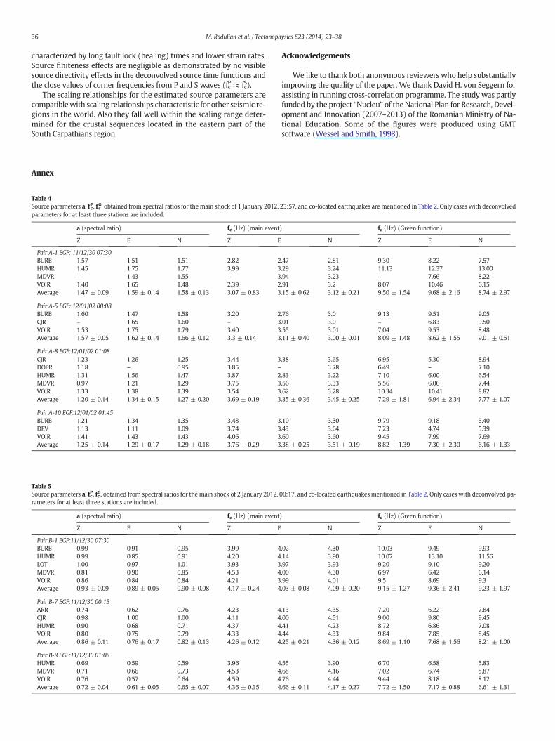
Spectral ratio method is applied for all the pairs, main event —empirical Green's function, that can be acquired from the tableabove. The source-related parameters in the theoretical function (1)are the asymptote at low frequency (in logarithmic scale), a, the cornerfrequency of main event, fcP, and the corner frequency of the EGF event,fcG. They are obtained by approximating the observed spectral ratio withthe theoretical one and by averaging the estimates for all the availableearthquake pairs and stations. We considered in our analysis only thecommon stations and station components with acceptable signal-to-noise ratio and only P waves. The estimations are given in Tables 4, 5and 6 (Annex) for the main events of 1st January 2012, 23:57, 2nd Jan-uary 2012, 00:17 and 2nd January 2012, 00:23, respectively. Examplesof spectral ratios computed for pairs of earthquakes are shown in Fig. 4.

Evidently, the low-frequency level, a, and the EGF corner frequency fcG

are depending on the particular earthquake pair, while the main eventcorner frequency fcP should not depend if source directivity effects arenegligible. The seismic moment is estimated for the main events using:

M0 ¼ 4πρvP3Ω0R

� �=Rθφ ð5Þ

ρ is the density at the source depth, vP is the velocity of Pwaves at sourcedepth, Ω0 is the long period displacement spectral level, R is the hypo-central distance and Rθφ is the source radiation pattern (average valuesof 0.52 for P waves and 0.63 for S waves, according to Aki and Richards,1980). We adopted for the study area the following parameters(Răileanu et al., 2012):

ρ ¼ 2:45g=cm3

vP ¼ 6:0km=skm=svS ¼ 3:47km=s:

Once the seismic moment estimates for the main events are obtain-ed, we use spectral ratio value at low frequency to estimate the seismicmoment for EGF earthquakes:

a ¼ logM0P=M0

G ¼ logΩ0P=Ω0

G ð6Þ

31M. Radulian et al. / Tectonophysics 623 (2014) 23–38

and

M0G ¼ M0

P=10a: ð7Þ

For the same pairs of co-located earthquakes we applied the decon-volution method with empirical Green's functions. The deconvolution iscarried out by spectral division for windows of 2–3 s of P-wave trainand 3–4 s of S-wave train. The windows are first 10% tapered. Then, tostabilize the spectral division, in case of spectral holes, the amplitudespectrum of EGF (which is denominator) is smoothed out, before divi-sion, with a five-point running moving window. In addition, to reducehigh-frequency instabilities, the deconvolved source time function isband-pass filtered between 0.5 and 10 Hz with a Butterworth filter.

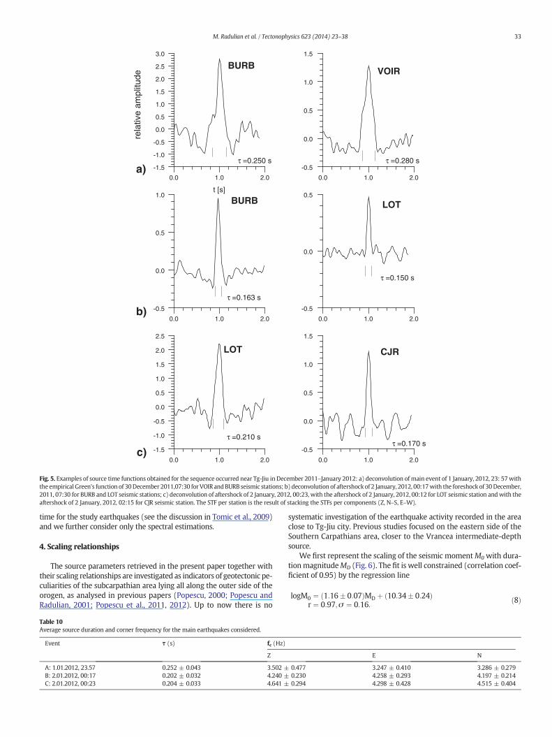
Examples of source time functions (STFs) are given in Fig. 5. In allcases, we can approximate STF by simple unipolar pulses. To smooth

-1.5 -1.0 -0.5 0.0 0.5 1.0 1.5

-1.5

-1.0

-0.5

0.0

0.5

1.0

1.5

2.0

2.5

-1.5

-1.0

-0.5

0.0

0.5

1.0

1.5

2.0

2.5

-1.5 -1.0 -0.5 0.0 0.5 1.0 1.5

-1.5

-1.0

-0.5

0.0

0.5

1.0

1.5

2.0

2.5

log

R

-1.5 -1.0 -0.5 0.0 0.5 1.0 1.5

log f (Hz)

BURBZ

E

N

Fig. 4. Spectral ratios obtained for following pairs: a) the main shock of 1 January, 2012, 23:57 aand 2 January, 1:08, MD = 3.2 for HUMR seismic station b) main shock of 2 January, 2012, 00:seismic station and 2 January, 00:12, MD = 2.5 for LOT seismic station.

small differences, the relative source time function for a given stationwas obtained by stacking the functions resulted after deconvolutionfrom all three components of that station. The source duration τ forthe threemain events is estimated from the STF. Since source directivityeffects are not visible, we use as estimate of source duration an averagevalue considering all the available stations for the EGFs associated withthe main shock.

Tables 7, 8 and 9 (Annex) contain the source duration values obtain-ed for themain event of 1 January, 2012, 23:57 whenever the STF pulsewas reasonably defined. Similar estimationswere achieved for the othertwo main events.

Finally, the estimations resulted after averaging over all stations andEGFs are given in Table 10. The ratio of P to S corner frequencies aver-aged over all stations is b fcP/fcSN = 1.07 for event A, 1.00 for event Band 1.04 for event C. A common value obtained in many studies is fcP/fcS

HUMR

-1.5

-1.0

-0.5

0.0

0.5

1.0

1.5

2.0

2.5

-1.5 -1.0 -0.5 0.0 0.5 1.0 1.5

-1.5

-1.0

-0.5

0.0

0.5

1.0

1.5

2.0

2.5

-1.5 -1.0 -0.5 0.0 0.5 1.0 1.5

-1.5

-1.0

-0.5

0.0

0.5

1.0

1.5

2.0

2.5

-1.5 -1.0 -0.5 0.0 0.5 1.0 1.5

a)

nd empirical Green’s functions of 30 December, 07:30, MD = 3.2 for BURB seismic station23, MD = 3.9 and empirical Green’s functions of 30 December, 07:30, MD = 3.2 for VOIR

-1.5 -1.0 -0.5 0.0 0.5 1.0 1.5 2.0

-1.5

-1.0

-0.5

0.0

0.5

1.0

1.5

2.0

2.5 LOT

-1.5

-1.0

-0.5

0.0

0.5

1.0

1.5

2.0

2.5

-1.5 -1.0 -0.5 0.0 0.5 1.0 1.5 2.0

-1.5

-1.0

-0.5

0.0

0.5

1.0

1.5

2.0

2.5

-1.5 -1.0 -0.5 0.0 0.5 1.0 1.5 2.0

-1.5

-1.0

-0.5

0.0

0.5

1.0

1.5

2.0

2.5

log

R

-1.5 -1.0 -0.5 0.0 0.5 1.0 1.5 2.0

log f (Hz)

VOIR

-1.5

-1.0

-0.5

0.0

0.5

1.0

1.5

2.0

2.5

-1.5 -1.0 -0.5 0.0 0.5 1.0 1.5 2.0

-1.5

-1.0

-0.5

0.0

0.5

1.0

1.5

2.0

2.5

-1.5 -1.0 -0.5 0.0 0.5 1.0 1.5 2.0

Z

E

N

b)

Fig. 4 (continued).

32 M. Radulian et al. / Tectonophysics 623 (2014) 23–38

~ 1.5 (e.g., Abercrombie and Leary, 1993; Molnar et al., 1973; Prietoet al., 2004; Viegas, 2012; Viegas et al., 2010) and is justified geometri-cally by the circular source model of Madariaga (1976). P-wave cornerfrequency is higher (P source pulse has shorter duration) because thetime elapsed between the arrival from the closest and more distantfault edge is smaller for P waves, than for S waves. The average 1.5value is expected for the waves leaving the fault at angles larger than30° from the fault normal. For radiation propagating close to the faultnormal direction, P and Swaves leave the source in phase and the inter-ference due to source finiteness is negligible (fcP ≈ fcS).

According to our results and within the unavoidable uncertainties,ratio fcP/fcS is around 1 and shows no azimuthal dependence. This is an in-dication that the spectra are dominated by the corner frequency con-trolled by the rise time (the same for both P and S waves), rather thanthe corner frequency controlled by the fault dimension (see Viegas,2012, for a similar case).

Based on seismic moment, corner frequency and source durationestimations, we determine the source area and stress drop using rela-tions (2)–(4). The results are presented in Table 11 for the mainevents and Table 12 for EGF events. The source radius estimated fromcorner frequency is an average between the estimations using P-waveand S-wave corner frequencies. Since relation (2) assumes a ratioabout 1.5 of fcP/fcS and for our data fcP ≈ fcS, the radius computed from fcP

is systematically greater than the radius computed from fcS roughly bya factor of 1.5 (for example, for event A, r = 317 m from fcP and r =223 m from fcS).

To apply Eq. (4), we adopted an average value of 30° for the take-offangle with respect to the fault normal. For θ varying between 0 and 45°,the variation in r is slightly higher than 30%.Weobtained systematic larg-er values for source radius, and correspondingly lower values for stressdrop, when using half of the source duration as compared with the spec-tral results. It is likely that the half duration is not a good proxy for the rise

0.0 1.0 2.0

t [s]

-1.5

-1.0

-0.5

0.0

0.5

1.0

1.5

2.0

2.5

3.0

rela

tive

ampl

itude

BURB

-0.5

0.0

0.5

1.0

1.5

0.0 1.0 2.0

-0.5

0.0

0.5

1.0

0.0 1.0 2.0

-1.5

-1.0

-0.5

0.0

0.5

1.0

1.5

2.0

2.5

0.0 1.0 2.0

-0.5

0.0

0.5

0.0 1.0 2.0

-0.5

0.0

0.5

1.0

1.5

0.0 1.0 2.0

τ =0.250 s

τ =0.163 s

τ =0.150 s

τ =0.280 s

τ =0.170 s τ =0.210 s

VOIR

BURB LOT

a)

b)

c)

CJRLOT

Fig. 5. Examples of source time functions obtained for the sequence occurred near Tg-Jiu in December 2011–January 2012: a) deconvolution of main event of 1 January, 2012, 23: 57withthe empirical Green’s function of 30December 2011,07:30 for VOIR andBURB seismic stations; b) deconvolution of aftershockof 2 January, 2012, 00:17with the foreshock of 30December,2011, 07:30 for BURB and LOT seismic stations; c) deconvolution of aftershock of 2 January, 2012, 00:23, with the aftershock of 2 January, 2012, 00:12 for LOT seismic station andwith theaftershock of 2 January, 2012, 02:15 for CJR seismic station. The STF per station is the result of stacking the STFs per components (Z, N–S, E–W).

33M. Radulian et al. / Tectonophysics 623 (2014) 23–38

time for the study earthquakes (see the discussion in Tomic et al., 2009)and we further consider only the spectral estimations.

4. Scaling relationships

The source parameters retrieved in the present paper together withtheir scaling relationships are investigated as indicators of geotectonic pe-culiarities of the subcarpathian area lying all along the outer side of theorogen, as analysed in previous papers (Popescu, 2000; Popescu andRadulian, 2001; Popescu et al., 2011, 2012). Up to now there is no

Table 10Average source duration and corner frequency for the main earthquakes considered.

Event τ (s) fc (Hz)

Z

A: 1.01.2012, 23.57 0.252 ± 0.043 3.502 ±B: 2.01.2012, 00:17 0.202 ± 0.032 4.240 ±C: 2.01.2012, 00:23 0.204 ± 0.033 4.641 ±

systematic investigation of the earthquake activity recorded in the areaclose to Tg-Jiu city. Previous studies focused on the eastern side of theSouthern Carpathians area, closer to the Vrancea intermediate-depthsource.

We first represent the scaling of the seismic momentM0 with dura-tionmagnitudeMD (Fig. 6). The fit is well constrained (correlation coef-ficient of 0.95) by the regression line

logM0 ¼ 1:16� 0:07ð ÞMD þ 10:34� 0:24ð Þr ¼ 0:97;σ ¼ 0:16:

ð8Þ

E N

0.477 3.247 ± 0.410 3.286 ± 0.2790.230 4.258 ± 0.293 4.197 ± 0.2140.294 4.298 ± 0.428 4.515 ± 0.404

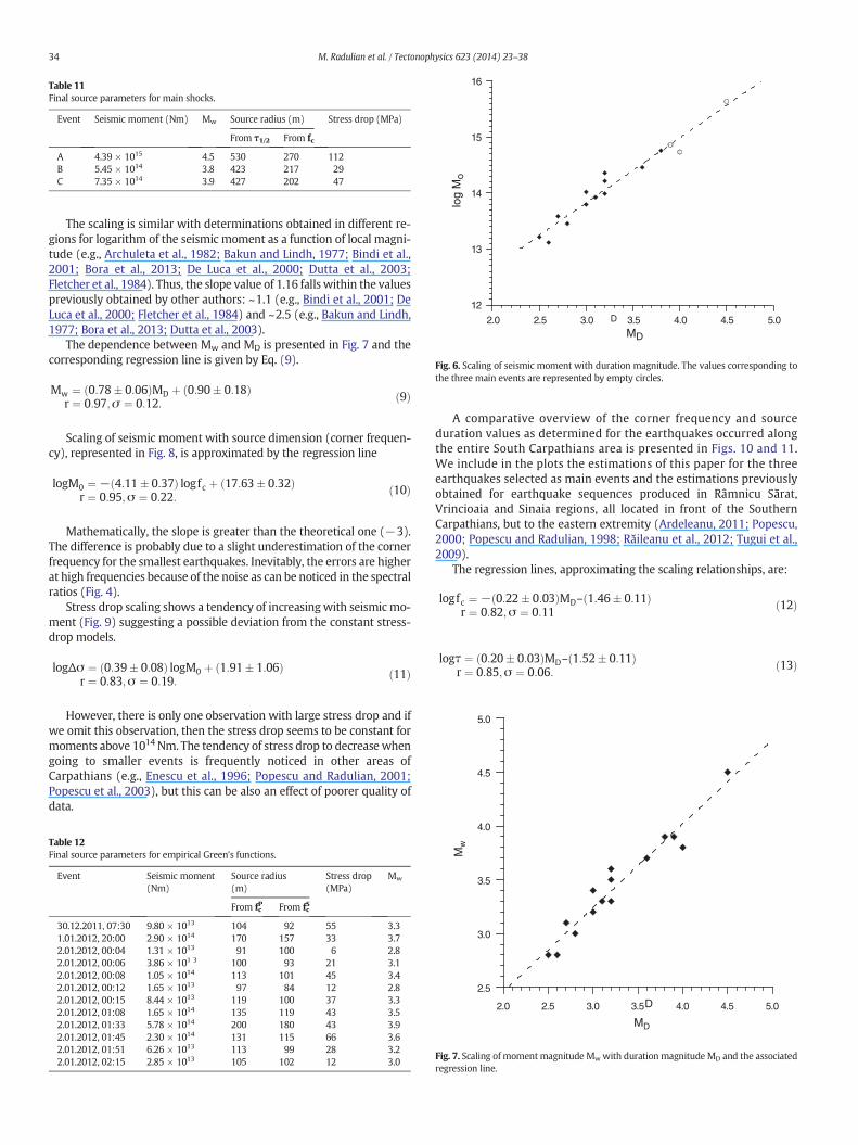
Table 11Final source parameters for main shocks.

Event Seismic moment (Nm) Mw Source radius (m) Stress drop (MPa)

From τ1/2 From fc

A 4.39 × 1015 4.5 530 270 112B 5.45 × 1014 3.8 423 217 29C 7.35 × 1014 3.9 427 202 47

2.0 2.5 3.0 3.5 4.0 4.5 5.0MD

12

13

14

15

16

log

Mo

D

Fig. 6. Scaling of seismic moment with duration magnitude. The values corresponding tothe three main events are represented by empty circles.

4.5

5.0

34 M. Radulian et al. / Tectonophysics 623 (2014) 23–38

The scaling is similar with determinations obtained in different re-gions for logarithm of the seismic moment as a function of local magni-tude (e.g., Archuleta et al., 1982; Bakun and Lindh, 1977; Bindi et al.,2001; Bora et al., 2013; De Luca et al., 2000; Dutta et al., 2003;Fletcher et al., 1984). Thus, the slope value of 1.16 falls within the valuespreviously obtained by other authors: ~1.1 (e.g., Bindi et al., 2001; DeLuca et al., 2000; Fletcher et al., 1984) and ~2.5 (e.g., Bakun and Lindh,1977; Bora et al., 2013; Dutta et al., 2003).

The dependence between Mw and MD is presented in Fig. 7 and thecorresponding regression line is given by Eq. (9).

Mw ¼ 0:78� 0:06ð ÞMD þ 0:90� 0:18ð Þr ¼ 0:97;σ ¼ 0:12: ð9Þ

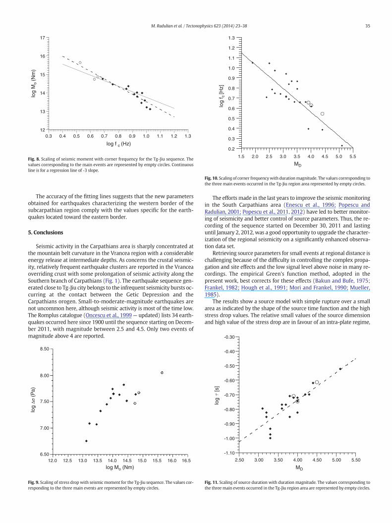
Scaling of seismic moment with source dimension (corner frequen-cy), represented in Fig. 8, is approximated by the regression line

logM0 ¼ − 4:11� 0:37ð Þ logfc þ 17:63� 0:32ð Þr ¼ 0:95;σ ¼ 0:22:

ð10Þ

Mathematically, the slope is greater than the theoretical one (−3).The difference is probably due to a slight underestimation of the cornerfrequency for the smallest earthquakes. Inevitably, the errors are higherat high frequencies because of the noise as can be noticed in the spectralratios (Fig. 4).

Stress drop scaling shows a tendency of increasingwith seismicmo-ment (Fig. 9) suggesting a possible deviation from the constant stress-drop models.

logΔσ ¼ 0:39� 0:08ð Þ logM0 þ 1:91� 1:06ð Þr ¼ 0:83;σ ¼ 0:19:

ð11Þ

However, there is only one observation with large stress drop and ifwe omit this observation, then the stress drop seems to be constant formoments above 1014 Nm. The tendency of stress drop to decreasewhengoing to smaller events is frequently noticed in other areas ofCarpathians (e.g., Enescu et al., 1996; Popescu and Radulian, 2001;Popescu et al., 2003), but this can be also an effect of poorer quality ofdata.

Table 12Final source parameters for empirical Green's functions.

Event Seismic moment(Nm)

Source radius(m)

Stress drop(MPa)

Mw

From fcP From fcS

30.12.2011, 07:30 9.80 × 1013 104 92 55 3.31.01.2012, 20:00 2.90 × 1014 170 157 33 3.72.01.2012, 00:04 1.31 × 1013 91 100 6 2.82.01.2012, 00:06 3.86 × 101 3 100 93 21 3.12.01.2012, 00:08 1.05 × 1014 113 101 45 3.42.01.2012, 00:12 1.65 × 1013 97 84 12 2.82.01.2012, 00:15 8.44 × 1013 119 100 37 3.32.01.2012, 01:08 1.65 × 1014 135 119 43 3.52.01.2012, 01:33 5.78 × 1014 200 180 43 3.92.01.2012, 01:45 2.30 × 1014 131 115 66 3.62.01.2012, 01:51 6.26 × 1013 113 99 28 3.22.01.2012, 02:15 2.85 × 1013 105 102 12 3.0

A comparative overview of the corner frequency and sourceduration values as determined for the earthquakes occurred alongthe entire South Carpathians area is presented in Figs. 10 and 11.We include in the plots the estimations of this paper for the threeearthquakes selected as main events and the estimations previouslyobtained for earthquake sequences produced in Râmnicu Sărat,Vrincioaia and Sinaia regions, all located in front of the SouthernCarpathians, but to the eastern extremity (Ardeleanu, 2011; Popescu,2000; Popescu and Radulian, 1998; Răileanu et al., 2012; Tugui et al.,2009).

The regression lines, approximating the scaling relationships, are:

logfc ¼ − 0:22� 0:03ð ÞMD– 1:46� 0:11ð Þr ¼ 0:82;σ ¼ 0:11

ð12Þ

logτ ¼ 0:20� 0:03ð ÞMD– 1:52� 0:11ð Þr ¼ 0:85;σ ¼ 0:06: ð13Þ

2.0 2.5 3.0 3.5 4.0 4.5 5.0

MD

2.5

3.0

3.5

4.0

Mw

D

Fig. 7. Scaling of momentmagnitude Mw with duration magnitude MD and the associatedregression line.

0.3 0.4 0.5 0.6 0.7 0.8 0.9 1.0 1.1 1.2 1.3

log f c (Hz)

12

13

14

15

16

17lo

g M

o (N

m)

Fig. 8. Scaling of seismic moment with corner frequency for the Tg-Jiu sequence. Thevalues corresponding to the main events are represented by empty circles. Continuousline is for a regression line of -3 slope.

1.5 2.0 2.5 3.0 3.5 4.0 4.5 5.0 5.5

MD

0.2

0.3

0.4

0.5

0.6

0.7

0.8

0.9

1.0

1.1

1.2

1.3

log

f c [H

z]

Fig. 10. Scaling of corner frequencywith durationmagnitude. The values corresponding tothe three main events occurred in the Tg-Jiu region area represented by empty circles.

-0.30

35M. Radulian et al. / Tectonophysics 623 (2014) 23–38

The accuracy of the fitting lines suggests that the new parametersobtained for earthquakes characterizing the western border of thesubcarpathian region comply with the values specific for the earth-quakes located toward the eastern border.

5. Conclusions

Seismic activity in the Carpathians area is sharply concentrated atthe mountain belt curvature in the Vrancea region with a considerableenergy release at intermediate depths. As concerns the crustal seismic-ity, relatively frequent earthquake clusters are reported in the Vranceaoverriding crust with some prolongation of seismic activity along theSouthern branch of Carpathians (Fig. 1). The earthquake sequence gen-erated close to Tg-Jiu city belongs to the infrequent seismicity bursts oc-curring at the contact between the Getic Depression and theCarpathians orogen. Small-to-moderate-magnitude earthquakes arenot uncommon here, although seismic activity is most of the time low.The Romplus catalogue (Oncescu et al., 1999— updated) lists 34 earth-quakes occurred here since 1900 until the sequence starting on Decem-ber 2011, with magnitude between 2.5 and 4.5. Only two events ofmagnitude above 4 are reported.

8.50

8.00

7.50

6.5012.5

7.00

12.0 13.513.0 14.514.0 15.515.0 16.516.0

log Mo (Nm)

log

Δσ (P

a)

Fig. 9. Scaling of stress drop with seismicmoment for the Tg-Jiu sequence. The values cor-responding to the three main events are represented by empty circles.

The efforts made in the last years to improve the seismicmonitoringin the South Carpathians area (Enescu et al., 1996; Popescu andRadulian, 2001; Popescu et al., 2011, 2012) have led to better monitor-ing of seismicity and better control of source parameters. Thus, the re-cording of the sequence started on December 30, 2011 and lastinguntil January 2, 2012, was a good opportunity to upgrade the character-ization of the regional seismicity on a significantly enhanced observa-tion data set.

Retrieving source parameters for small events at regional distance ischallenging because of the difficulty in controlling the complex propa-gation and site effects and the low signal level above noise in many re-cordings. The empirical Green's function method, adopted in thepresent work, best corrects for these effects (Bakun and Bufe, 1975;Frankel, 1982; Hough et al., 1991; Mori and Frankel, 1990; Mueller,1985).

The results show a source model with simple rupture over a smallarea as indicated by the shape of the source time function and the highstress drop values. The relative small values of the source dimensionand high value of the stress drop are in favour of an intra-plate regime,

MD

log

[s]

2.50 3.00 3.50 4.00 4.50 5.00 5.50

-1.10

-1.00

-0.90

-0.80

-0.70

-0.60

-0.50

-0.40

Fig. 11. Scaling of source duration with duration magnitude. The values corresponding tothe threemain events occurred in the Tg-Jiu region area are represented by empty circles.

36 M. Radulian et al. / Tectonophysics 623 (2014) 23–38

characterized by long fault lock (healing) times and lower strain rates.Source finiteness effects are negligible as demonstrated by no visiblesource directivity effects in the deconvolved source time functions andthe close values of corner frequencies from P and S waves (fcP ≈ fcS).

The scaling relationships for the estimated source parameters arecompatiblewith scaling relationships characteristic for other seismic re-gions in the world. Also they fall well within the scaling range deter-mined for the crustal sequences located in the eastern part of theSouth Carpathians region.

Table 4Source parameters a, fcP, fcG, obtained from spectral ratios for themain shock of 1 January 2012,parameters for at least three stations are included.

a (spectral ratio) fc (Hz) (main event

Z E N Z E

Pair A-1 EGF: 11/12/30 07:30BURB 1.57 1.51 1.51 2.82 2HUMR 1.45 1.75 1.77 3.99 3MDVR – 1.43 1.55 – 3VOIR 1.40 1.65 1.48 2.39 2Average 1.47 ± 0.09 1.59 ± 0.14 1.58 ± 0.13 3.07 ± 0.83 3

Pair A-5 EGF: 12/01/02 00:08BURB 1.60 1.47 1.58 3.20 2CJR – 1.65 1.60 – 3VOIR 1.53 1.75 1.79 3.40 3Average 1.57 ± 0.05 1.62 ± 0.14 1.66 ± 0.12 3.3 ± 0.14 3

Pair A-8 EGF:12/01/02 01:08CJR 1.23 1.26 1.25 3.44 3DOPR 1.18 – 0.95 3.85 –

HUMR 1.31 1.56 1.47 3.87 2MDVR 0.97 1.21 1.29 3.75 3VOIR 1.33 1.38 1.39 3.54 3Average 1.20 ± 0.14 1.34 ± 0.15 1.27 ± 0.20 3.69 ± 0.19 3

Pair A-10 EGF:12/01/02 01:45BURB 1.21 1.34 1.35 3.48 3DEV 1.13 1.11 1.09 3.74 3VOIR 1.41 1.43 1.43 4.06 3Average 1.25 ± 0.14 1.29 ± 0.17 1.29 ± 0.18 3.76 ± 0.29 3

Table 5Source parameters a, fcP, fcG, obtained from spectral ratios for the main shock of 2 January 2012,rameters for at least three stations are included.

a (spectral ratio) fc (Hz) (main event

Z E N Z E

Pair B-1 EGF:11/12/30 07:30BURB 0.99 0.91 0.95 3.99 4HUMR 0.99 0.85 0.91 4.20 4LOT 1.00 0.97 1.01 3.93 3MDVR 0.81 0.90 0.85 4.53 4VOIR 0.86 0.84 0.84 4.21 3Average 0.93 ± 0.09 0.89 ± 0.05 0.90 ± 0.08 4.17 ± 0.24 4

Pair B-7 EGF:11/12/30 00:15ARR 0.74 0.62 0.76 4.23 4CJR 0.98 1.00 1.00 4.11 4HUMR 0.90 0.68 0.71 4.37 4VOIR 0.80 0.75 0.79 4.33 4Average 0.86 ± 0.11 0.76 ± 0.17 0.82 ± 0.13 4.26 ± 0.12 4

Pair B-8 EGF:11/12/30 01:08HUMR 0.69 0.59 0.59 3.96 4MDVR 0.71 0.66 0.73 4.53 4VOIR 0.76 0.57 0.64 4.59 4Average 0.72 ± 0.04 0.61 ± 0.05 0.65 ± 0.07 4.36 ± 0.35 4

Annex

Acknowledgements

We like to thank both anonymous reviewers who help substantiallyimproving the quality of the paper. We thank David H. von Seggern forassisting in running cross-correlation programme. The study was partlyfunded by the project “Nucleu” of the National Plan for Research, Devel-opment and Innovation (2007–2013) of the Romanian Ministry of Na-tional Education. Some of the figures were produced using GMTsoftware (Wessel and Smith, 1998).

23:57, and co-located earthquakes are mentioned in Table 2. Only cases with deconvolved

) fc (Hz) (Green function)

N Z E N

.47 2.81 9.30 8.22 7.57

.29 3.24 11.13 12.37 13.00

.94 3.23 – 7.66 8.22

.91 3.2 8.07 10.46 6.15

.15 ± 0.62 3.12 ± 0.21 9.50 ± 1.54 9.68 ± 2.16 8.74 ± 2.97

.76 3.0 9.13 9.51 9.05

.01 3.0 – 6.83 9.50

.55 3.01 7.04 9.53 8.48

.11 ± 0.40 3.00 ± 0.01 8.09 ± 1.48 8.62 ± 1.55 9.01 ± 0.51

.38 3.65 6.95 5.30 8.943.78 6.49 – 7.10

.83 3.22 7.10 6.00 6.54

.56 3.33 5.56 6.06 7.44

.62 3.28 10.34 10.41 8.82

.35 ± 0.36 3.45 ± 0.25 7.29 ± 1.81 6.94 ± 2.34 7.77 ± 1.07

.10 3.30 9.79 9.18 5.40

.43 3.64 7.23 4.74 5.39

.60 3.60 9.45 7.99 7.69

.38 ± 0.25 3.51 ± 0.19 8.82 ± 1.39 7.30 ± 2.30 6.16 ± 1.33

00:17, and co-located earthquakesmentioned in Table 2. Only cases with deconvolved pa-

) fc (Hz) (Green function)

N Z E N

.02 4.30 10.03 9.49 9.93

.14 3.90 10.07 13.10 11.56

.97 3.93 9.20 9.10 9.20

.00 4.30 6.97 6.42 6.14

.99 4.01 9.5 8.69 9.3

.03 ± 0.08 4.09 ± 0.20 9.15 ± 1.27 9.36 ± 2.41 9.23 ± 1.97

.13 4.35 7.20 6.22 7.84

.00 4.51 9.00 9.80 9.45

.41 4.23 8.72 6.86 7.08

.44 4.33 9.84 7.85 8.45

.25 ± 0.21 4.36 ± 0.12 8.69 ± 1.10 7.68 ± 1.56 8.21 ± 1.00

.55 3.90 6.70 6.58 5.83

.68 4.16 7.02 6.74 5.87

.76 4.44 9.44 8.18 8.12

.66 ± 0.11 4.17 ± 0.27 7.72 ± 1.50 7.17 ± 0.88 6.61 ± 1.31

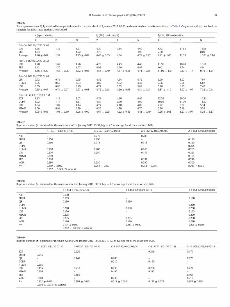
Table 6Source parameters a, fcP, fcG, obtained from spectral ratios for the main shock of 2 January 2012, 00:23, and co-located earthquakesmentioned in Table 2. Only cases with deconvolved pa-rameters for at least two stations are included.

a (spectral ratio) fc (Hz) (main event) fc (Hz) (Green function)

Z E N Z E N Z E N

Pair C-4 EGF:11/12/30 00:06LOT 1.28 1.32 1.27 4.20 4.34 4.60 8.42 11.53 12.05SRE 1.23 – 1.22 4.70 – 4.98 7.00 8.00Average 1.26 ± 0.04 1.32 1.25 ± 0.04 4.45 ± 0.35 4.34 4.79 ± 0.27 7.71 ± 1.00 11.53 10.03 ± 2.86

Pair C-6 EGF:11/12/30 00:12LOT 1.70 1.62 1.76 4.23 4.43 4.46 11.91 10.20 10.61SRE 1.42 1.70 1.67 4.93 4.90 4.96 10.2 8.54 8.9Average 1.56 ± 0.20 1.66 ± 0.06 1.72 ± 0.06 4.58 ± 0.49 4.67 ± 0.33 4.71 ± 0.35 11.06 ± 1.21 9.37 ± 1.17 9.76 ± 1.21

Pair C-8 EGF:11/12/30 01:08CJR 0.72 0.76 0.75 4.52 4.54 4.72 6.90 8.02 7.67HUMR 0.65 0.67 0.64 4.87 4.52 4.42 7.96 5.88 6.87LOT 0.59 0.80 0.79 4.77 3.53 3.88 5.76 6.85 7.42Average 0.65 ± 0.07 0.74 ± 0.07 0.73 ± 0.08 4.72 ± 0.18 4.20 ± 0.58 4.34 ± 0.43 6.87 ± 1.10 6.92 ± 1.07 7.32 ± 0.41

Pair C-11 EGF:11/12/30 01:51BZS 1.13 1.13 1.03 4.78 4.36 4.95 12.36 10.50 10.84DOPR 1.02 1.17 1.17 4.84 3.70 4.00 10.50 11.30 11.50LOT 1.04 1.07 1.14 4.77 4.10 4.00 7.22 5.27 5.34MDVR 1.00 0.94 0.99 4.30 4.70 4.70 6.96 5.99 5.36Average 1.05 ± 0.06 1.08 ± 0.10 1.08 ± 0.09 4.67 ± 0.25 4.22 ± 0.42 4.41 ± 0.49 9.26 ± 2.63 8.27 ± 3.07 8.26 ± 3.37

Table 7Rupture duration (τ) obtained for the main event of 1st January 2012, 23:57, MD = 4.5 as average for all the associated EGFs.

A-1 EGF 11/12/30 07:30 A-5 EGF 12/01/02 00:08 A-7 EGF 12/01/02 00:15 A-8 EGF 12/01/02 01:08

ARR - 0.270 0.288 –

BURB 0.250 0.190 – 0.180CJR 0.290 0.275 0.315 0.320DOPR – – – 0.278HUMR 0.270 0.260 0.260 0.265LOT 0.270 0.250 0.175 0.223MDVR 0.240 – – 0.164SRE 0.210 – 0.197 0.240VOIR 0.280 0.280 0.290 0.300Av 0.259 ± 0.027 0.254 ± 0.033 0.254 ± 0.056 0.246 ± 0.055

0.252 ± 0.043 (27 values)

Table 8Rupture duration (τ) obtained for the main event of 2nd January 2012, 00:17, MD = 4.0 as average for all the associated EGFs.

B-1 EGF 11/12/30 07:30 B-6 EGF 12/01/02 00:15 B-8 EGF 12/01/02 01:08

ARR 0.190 – –

BURB 0.163 – 0.180CJR 0.190 0.190 –

DOPR – – 0.230HUMR 0.210 0.180 0.230LOT 0.150 – 0.163MDVR 0.225 – 0.220SRE 0.235 0.285 0.200VOIR 0.190 0.190 0.220Av 0.194 ± 0.029 0.211 ± 0.049 0.206 ± 0.026

0.202 ± 0.032 (19 values)

Table 9Rupture duration (τ) obtained for the main event of 2nd January 2012, 00:23, MD = 3.9 as average for all the associated EGFs.

C-1 EGF 11/12/30 07:30 C-6 EGF:12/01/02 00:12 C-8 EGF:12/01/02 01:08 C-11 EGF:12/01/02 01:51 C-12 EGF:12/01/02 02:15

BZS – 0.220 – 0.240 0.170BURB 0.245 – – – –

CJR – 0.140 0.200 – 0.170DOPR – – 0.210 0.155 –

HUMR 0.255 – – – –

LOT 0.195 0.210 0.230 0.200 0.222MDVR 0.205 – 0.190 0.212 –

SRE – 0.150 – – 0.167VOIR 0.260 – 0.230 – 0.210Av 0.232 ± 0.030 0.180 ± 0.040 0.212 ± 0.018 0.192 ± 0.025 0.188 ± 0.026

0.204 ± 0.033 (23 values)

37M. Radulian et al. / Tectonophysics 623 (2014) 23–38

38 M. Radulian et al. / Tectonophysics 623 (2014) 23–38

References

Abercrombie, R.E., Leary, P.C., 1993. Source parameters of small earthquakes recorded at2.5 km depth, Cajon Pass, southern California: implications for earthquake scaling.Geophys. Res. Lett. 20, 1511–1514.

Aki, K., Richards, P., 1980. Quantitative Seismology: Theory and Methods. Freeman, SanFrancisco (932 pp.).

Archuleta, R.J., Cranswick, E.C., Muller, C., Spudich, P., 1982. Source parameters of the 1980Mammoth Lakes, California, earthquakes sequence. J. Geophys. Res. 87, 4595–4607.

Ardeleanu, L., 2011. Reliability of source parameters of low magnitude crustal earth-quakes of Vrancea retrieved by high frequency waveform inversion. Rom. J. Phys.56, 827–841.

Bakun, W.H., Bufe, C.G., 1975. Shear-wave attenuation along the San Andreas Fault zonein Central California. Bull. Seismol. Soc. Am. 65, 439–460.

Bakun, W.H., Lindh, A.G., 1977. Local magnitudes, seismic moments and coda duration forearthquakes near Oroville, California. Bull. Seismol. Soc. Am. 67, 615–629.

Bindi, D., Spallarossa, D., Augliera, P., Cattaneo, M., 2001. Source parameters estimatedfrom the aftershocks of the 1997 Umbria–Marche (Italy) seismic sequence. Bull.Seismol. Soc. Am. 91, 448–455.

Boatwright, J., 1980. A spectral theory for circular seismic sources: simple estimates ofsource duration, dynamic stress drop, and radiated energy. Bull. Seismol. Soc. Am.70, 1–28.

Bora, D.K., Baruah, S., Biswas, R., Gogoi, N.K., 2013. Estimation of source parameters oflocal earthquakes originated in Shillong–Mikir Plateau and its adjoining region ofNortheastern India. Bull. Seismol. Soc. Am. 103, 437–446.

Brune, J.N., 1970. Tectonic stress and the spectra of seismic shear waves from earth-quakes. J. Geophys. Res. 75, 4997–5009.

De Luca, G., Scarpa, R., Filippi, L., Gorini, A., Marcucci, S., Marsan, P., Milna, G., Zambonelli,E., 2000. A detailed analysis of two seismic sequences in Abruzzo, central Apennines,Italy. J. Seismol. 4, 1–21.

Dutta, U., Biswas, N., Martirosyan, A., Papageorgiou, A., Kinoshita, S., 2003. Estimation ofearthquake source parameters and site response in Anchorage, Alaska, from strong-motion network data using generalized inversion method. Phys. Earth Planet. Inter.137, 13–29.

Enescu, D., Popescu, E., Radulian, M., 1996. Source characteristics of the Sinaia (Romania)sequence of May–June 1993. Tectonophysics 261, 39–49.

Fletcher, J., Boatwright, J., Haar, L., Hanks, L., McGarr, A., 1984. Source parameters for after-shocks of the Oroville, California, earthquake. Bull. Seismol. Soc. Am. 74, 1101–1123.

Frankel, A., 1982. Precursors to a magnitude 4.8 earthquake in the Virgin Islands: spatialclustering of small earthquakes, anomalous focal mechanisms, and earthquake dou-blets. Bull. Seismol. Soc. Am. 72, 1277–1294.

Frankel, A., Flechter, J., Vernon, F., Haar, L., Berger, J., Hanks, T., Brune, J., 1986. Rupturecharacteristics and tomography source imaging of ML = 3 earthquakes near Anza,Southern California. J. Geophys. Res. 91, 12633–12650.

Havskov, J., Ottemöller, L., 2001. SEISAN: The Earthquake Analysis Software, Version 7.2.University of Bergen, Norway (256 pp.).

Hough, S.E., Seeber, L., Lerner-Lam, A., Armbruster, G., Guo, H., 1991. Empirical Green'sfunction analysis of Loma Prieta aftershocks. Bull. Seismol. Soc. Am. 81, 1737–1753.

Imanishi, K., Ellsworth, W.L., 2006. Source scaling relationships of microearthquakes atParkfield, CA, determined using the SAFOD pilot hole seismic array. In:Abercrombie, R.E., McGarr, A., Kanamori, H., Di Toro, G. (Eds.), Earthquakes: radiatedenergy and the physics of faulting. Geophysical Monograph Series, vol. 170. AmericanGeophysical Union, Washington, D.C., pp. 81–90.

Krézsek, C., Lăpădat, A., Maţenco, L., Arnberger, K., Barbu, V., Olaru, R., 2013. Strainpartitioning at orogenic contacts during rotation, strike–slip and oblique conver-gence: Paleogene–Early Miocene evolution of the contact between the SouthCarpathians and Moesia. Glob. Planet. Chang. 103, 63–81.

Lindley, G.T., 1994. Source parameters of the 23 April 1992 Joshua Tree, California earth-quake, its largest foreshock and aftershocks. Bull. Seismol. Soc. Am. 84, 1051–1057.

Madariaga, R., 1976. Dynamics of an expanding circular crack. Bull. Seismol. Soc. Am. 66,639–666.

Maţenco, L., Zoetemeijer, R., Cloetingh, S., Dinu, C., 1997a. Lateral variations inmechanicalproperties of the Romanian external Carpathians: inferences of flexure and gravitymodeling. Tectonophysics 282, 147–166.

Maţenco, L., Bertotti, G., Dinu, C., Cloetingh, S., 1997b. Tertiary tectonic evolution of theexternal South Carpathians and the adjacent Moesian platform (Romania). Tectonics16 (6), 896–911.

Matenco, L., Krezsek, C., Merten, S., Schmid, S., Cloetingh, S., Andriessen, P., 2010. Charac-teristics of collisional orogens with low topographic build-up: an example from theCarpathians. Terra Nova 22, 155–165.

Molnar, P., Tucker, B.E., Brune, J., 1973. Corner frequencies of P and S wave and models ofearthquake sources. Bull. Seismol. Soc. Am. 63, 2091–2104.

Mori, J., Frankel, A., 1990. Source parameters for small events associated with the 1986North Palm Springs, California earthquake determined using empirical Green func-tions. Bull. Seismol. Soc. Am. 80, 278–285.

Mueller, C.S., 1985. Source pulse enhancement by deconvolution of an empirical Green'sfunction. Geophys. Res. Lett. 12, 33–36.

Oncescu, M.C., Mârza, V., Rizescu, M., Popa, M., 1999. The Romanian earthquakescatalogue between 984 and 1997. In: Wenzel, F., Lungu, D. (Eds.), VranceaEarthquakes: Tectonics, Hazard and Risk Mitigation. Kluwer Academic Publishers,pp. 43–47 (continuously updated).

Polonic, G., 1996. Structure of the crystalline basement in Romania. Rev. Roum. Geophys.40, 57–69.

Popescu, E., 2000. Complex study of the earthquake sequences on the Romanian territory.(PhD Thesis) Institute of Atomic Physics, Bucharest (281 pp. (in Romanian)).

Popescu, E., Radulian, M., 1998. Source complexity of the crustal earthquake sequences inthe Eastern Carpathians foredeep area. Rom. J. Phys. 43, 837–850.

Popescu, E., Radulian, M., 2001. Source characteristics of the seismic sequences in theEastern Carpathians foredeep region (Romania). Tectonophysics 338, 325–337.

Popescu, E., Popa, M., Radulian, M., 2003. Efficiency of the spectral ratio method to con-strain the source scaling properties of the Vrancea (Romania) subcrustal earthquakes.Rom. Rep. Phys. 55, 149–169.

Popescu, E., Neagoe, C., Rogozea, M., Moldovan, I.A., Borleanu, F., Radulian, M., 2011.Source parameters for the earthquake sequence occurred in the Ramnicu Sarat area(Romania) November–December 2007. Rom. J. Phys. 56, 265–278.

Popescu, E., Borleanu, F., Rogozea, M., Radulian, M., 2012. Source analysis for earthquakesequence occurred in Vrancea (Romania) region on 6 to 30 September 2008. Rom.Rep. Phys. 64, 571–590.

Prieto, G.A., Shearer, P.M., Vernon, F.L., Kilb, D., 2004. Earthquake source scaling and self-similarity estimation from stacking P and S spectra. J. Geophys. Res. 109 (B0), 8310.http://dx.doi.org/10.1029/2004JB003084.

Răbăgia, T., Matenco, L., Cloetingh, S., 2011. The interplay between eustacy, tectonics andsurface processes during the growth of a fault-related structure as derived from se-quence stratigraphy: the Govora–Ocnele Mari antiform, South Carpathians.Tectonophysics 502, 196–220.

Radulian, M., Mândrescu, N., Panza, G.F., Popescu, E., Utale, A., 2000. Characterization ofRomanian seismogenic zones. In: Panza, G.F., Radulian, M., Trifu, C.I. (Eds.), SeismicHazard of the Circum-Pannonian Region. Pure Appl. Geophys, 157, pp. 57–77.

Răileanu, V., Tătaru, D., Grecu, B., 2012. Crustal models in Romania— I. Moesian platform.Rom. Rep. Phys. 64, 539–554.

Săndulescu, M., 1984. Geotectonics of Romania. Ed. Tehnică, Bucharest (334 pp.(in Romanian)).

Săndulescu,M., 1988. Cenozoic tectonic history of theCarpathians. In: Royden, L.H., Horváth,F. (Eds.), The Pannonian Basin, a study in basin evolution. AAPG Mem., 45, pp. 17–25.

Schmid, S.M., Bernoulli, D., Fügenschuh, B., Matenco, M., Schefer, S., Schuster, R., Tischler,M., Ustaszewski, K., 2008. The Alps–Carpathians–Dinarides-connection: a correlationof tectonic units. Swiss J. Geosci. 101, 139–183.

Tomic, J., Abercrombie, R.E., do Nascimento, A.F., 2009. Source parameters and rupture ve-locity of small M ≤ 2.1 reservoir induced earthquakes. Geophys. J. Int. 179,1013–1023.

Tugui, A., Craiu, M., Rogozea, M., Popa, M., Radulian, M., 2009. Seismotectonics of Vrancea(Romania) zone: the case of crustal seismicity in the foredeep area. Rom. Rep. Phys.61, 325–334.

Viegas, G.L., 2012. Source parameters of the 16 July 2010 Mw 3.4 Germantown, Maryland,earthquake. Seismol. Res. Lett. 83, 933–944.

Viegas, G., Baise, L., Abercrombie, R.E., 2010. Regional wave propagation in New Englandand New York. Bull. Seismol. Soc. Am. 100, 2196–2218.

Waldhauser, F., 2001. HypoDD: a program to compute double-difference hypocenterlocations (hypoDD version 1.0-03/2001). U.S. Geol. Surv. Open File Rept. 01-113.

Waldhauser, F., Ellsworth,W.L., 2000. A double-difference earthquake location algorithm:method and application to the Northern Hayward Fault, California. Bull. Seismol. Soc.Am. 90, 1353–1368.

Wessel, P., Smith, W.H.F., 1998. New improved version of the Generic Mapping Toolsreleased. EOS Trans. Am. Geophys. Union 79, 579.