South Atlantic Ocean cyclogenesis climatology simulatedby regional climate model (RegCM3)

Michelle Simoes Reboita Æ Rosmeri Porfırio da Rocha ÆTercio Ambrizzi Æ Shigetoshi Sugahara

Received: 19 March 2009 / Accepted: 10 September 2009

� Springer-Verlag 2009

Abstract A detailed climatology of the cyclogenesis over

the Southern Atlantic Ocean (SAO) from 1990 to 1999 and

how it is simulated by the RegCM3 (Regional Climate

Model) is presented here. The simulation used as initial and

boundary conditions the National Centers for Environ-

mental Prediction—Department of Energy (NCEP/DOE)

reanalysis. The cyclones were identified with an automatic

scheme that searches for cyclonic relative vorticity (f10)

obtained from a 10-m height wind field. All the systems

with f10 B -1.5 9 10-5 s-1 and lifetime equal or larger

than 24 h were considered in the climatology. Over SAO,

in 10 years were detected 2,760 and 2,787 cyclogeneses in

the simulation and NCEP, respectively, with an annual

mean of 276.0 ± 11.2 and 278.7 ± 11.1. This result sug-

gests that the RegCM3 has a good skill to simulate the

cyclogenesis climatology. However, the larger model

underestimations (-9.8%) are found for the initially

stronger systems (f10 B -2.5 9 10-5 s-1). It was noted

that over the SAO the annual cycle of the cyclogenesis

depends of its initial intensity. Considering the systems

initiate with f10 B -1.5 9 10-5 s-1, the annual cycle is

not well defined and the higher frequency occurs in the

autumn (summer) in the NCEP (RegCM3). The stronger

systems (f10 B -2.5 9 10-5 s-1) have a well-characterized

high frequency of cyclogenesis during the winter in both

NCEP and RegCM3. This work confirms the existence of

three cyclogenetic regions in the west sector of the SAO,

near the South America east coast and shows that RegCM3

is able to reproduce the main features of these cyclogenetic

areas.

Keywords Cyclogenesis � South Atlantic Ocean �Climate simulation � RegCM3

1 Introduction

Extratropical cyclones are formed and or intensify in some

preferential regions of the globe: to the lee side of the

mountains, regions of strong temperature gradients, coastal

areas, etc. These systems can affect the weather over the

regions where they act through cloud formation, precipi-

tation, strong winds and temperature change (Palmen and

Newton 1969). The strong winds over the ocean favor the

air–sea momentum transfer that is responsible for the ocean

disturbance which may lead to the occurrence of the high

sea waves causing problems to the navigation, petroleum

platforms, and severe shore erosion. On the other hand,

extratropical cyclones have a central role on the global

climate equilibrium, acting in large proportion in the

atmosphere heat, water vapor and momentum transport

towards the poles (Peixoto and Oort 1992). Therefore, a

better acknowledge of the behavior of these systems in

terms of their formation, frequency, trajectory and intensity

M. S. Reboita (&) � R. P. da Rocha � T. Ambrizzi

Department of Atmospheric Sciences, Institute of Astronomy,

Geophysics and Atmospheric Sciences, University of Sao Paulo,

Rua do Matao, 1226, Cidade Universitaria, Sao Paulo,

SP 05508900, Brazil

e-mail: reboita@model.iag.usp.br

R. P. da Rocha

e-mail: rosmerir@model.iag.usp.br

T. Ambrizzi

e-mail: ambrizzi@model.iag.usp.br

S. Sugahara

Institute of Meteorological Researches and Sciences Faculty,

Sao Paulo State University, Campus Bauru, Av. Luiz Edmundo

C. Coube s/n, Vargem Limpa, Caixa Postal 281, Bauru,

SP 17001-970, Brazil

e-mail: shige@ipmet.unesp.br

123

Clim Dyn

DOI 10.1007/s00382-009-0668-7

may be useful for their prediction, minimizing economic

loss or even lives.

Climatological studies of extratropical cyclones over

South America and adjacent oceans have been done by

many authors using different methodologies to identify and

tracking these systems. Necco (1982a, b) identified the

systems using near surface streamlines analysis and Gan

and Rao (1991) using minimum mean sea level pressure

(MSLP) over synoptic charts; Satyamurty et al. (1990)

identifying vortices in satellite images; Sinclair (1996) and

Reboita et al. (2005) have used cyclonic relative vorticity

from global reanalysis. Gan and Rao (1991) found two

preferential regions of cyclogenesis over the east coast of

South America: one on the southeastern coast of Argentina

(*42�S), and other in the Uruguay coast. Some other

authors (i.e. Sinclair 1996; Hoskins and Hodges 2005) also

found large occurrence of systems on the south/southeast-

ern coast of Brazil (*25�S).

There have been many studies (Lambert 1988, 1995;

Murray and Simmonds 1991; Konig et al. 1993; Hodges

1994, 1996) performing cyclone tracking in simulations of

the present climate using atmospheric global circulation

models (GCM) in order to verify their skill once synoptic

systems involve complex interactions with different spatial

and temporal scales, being an efficient way to validate

them (Sinclair and Watterson 1999). Other authors (Zhang

and Wang 1997; Hudson and Hewitson 1997; Hudson

1997; Blender et al. 1997; Sinclair and Watterson 1999;

Fyfe 2003; Raible and Blender 2004; Watterson 2006)

have investigated the cyclone climatology in GCM simu-

lations of future climate considering the increase of the

greenhouse gases (IPCC 2007).

A fundamental issue concerning the use of GCM to

provide regional climate scenarios is about horizontal

resolution. GCM are still run at horizontal grid intervals of

100–300 km. While this resolution is sufficient to capture

the large scale processes of the climate (Giorgi and Mearns

1991), it is not suitable for finer regional and local scales.

One alternative to that was originally proposed by

Dickinson et al. (1989) and Giorgi (1990). They suggested

to use limited area models or as it is known nowadays,

Regional Climate Models (RCM). This idea was based on

the concept of one way nesting, in which large scale

meteorological fields from GCM runs provide initial and

time-dependent meteorological lateral boundary conditions

for RCM simulations.

Many previous studies have already used RCM to simu-

late some climate features over South America (Seth and

Rojas 2003; Fernandez et al. 2006; Pal et al. 2007), but

most of them were not concerned about extratropical

cyclonic systems and how skillful the RCM are to simulate

their climatology. More recently, Lionello et al. (2008)

analyzed the cyclone climatology over Europa, using the

RegCM3 to simulate the present (1961–1990) and future

climate (2071–2100). When compared to the European

Centre of Medium Range Weather Forecasting (ECMWF;

Uppala et al. 2005) reanalysis data the RegCM3 was able

to reproduce the main cyclones climatological features,

particularly their spatial distribution.

The main objective of this study is to evaluate the ability

of the RegCM3 in simulate the cyclone climatology on the

large part of South Atlantic Ocean (between 15� and 55�S)

in the period 1990–1999. Knowing the strength and limi-

tations of the RegCM3 to simulate the present climate is

important if one wants to use this model in projections of

future climate scenarios. This paper is organized as follow:

Sect. 2 briefly describes the RegCM3, the simulation main

features, data used, the cyclone tracking scheme and the

analysis to be done. The results are presented in Sect. 3 and

some concluding remarks are given in Sect. 4.

2 Regional model, data and methodology

2.1 RegCM3 description

The RegCM3 limited area model has the dynamical core

based on the hydrostatic version of the National Center for

Atmospheric Research-Pennsylvania State University

(NCAR-PSU) Mesoscale Model version 5 (Pal et al. 2007).

RegCM3 is a primitive equation, compressible and in

sigma-pressure vertical coordinate model.

The RegCM3 surface physics processes are obtained

using the Biosphere–Atmosphere Transfer Scheme (BATS

version 1e, Dickinson et al. 1993). This scheme describes

the role of the vegetation (or water) in the modification of

the moment, energy and water vapor fluxes exchange

between surface and atmosphere. In the formulation of the

planetary boundary layer, the turbulent transport of energy,

moment, and moisture results from the product between

their vertical gradient and the coefficient of turbulent ver-

tical diffusion, with a non-local turbulent formulation

proposed by Holtslag et al. (1990). Over the ocean the

surface turbulent fluxes can be calculated following Zeng

et al. (1998), where the roughness length is a function of

the atmospheric stability and near surface wind intensity.

The NCAR CCM3 (Community Climate Model 3; Kiehl

et al. 1996) radiative transfer scheme is used in the Reg-

CM3. The precipitation is represented in two forms: grid-

scale (resolvable scale) and convective (subgrid-scale). The

grid-scale precipitation scheme (Pal et al. 2000) only

considers the water phase and includes formulations for

auto-conversion of cloud water into rainwater, accretion of

cloud droplets by falling raindrops, and evaporation of

falling raindrops. Three options are available to represent

cumulus convection: (1) the modified Anthes-Kuo scheme

M. S. Reboita et al.: South Atlantic Ocean cyclogenesis climatology

123

(Anthes 1977; Giorgi 1991); (2) the Grell scheme (Grell

1993); and (3) the Massachusetts Institute of Technology

(MIT) scheme (Emanuel 1991).

2.2 Numerical simulation and data

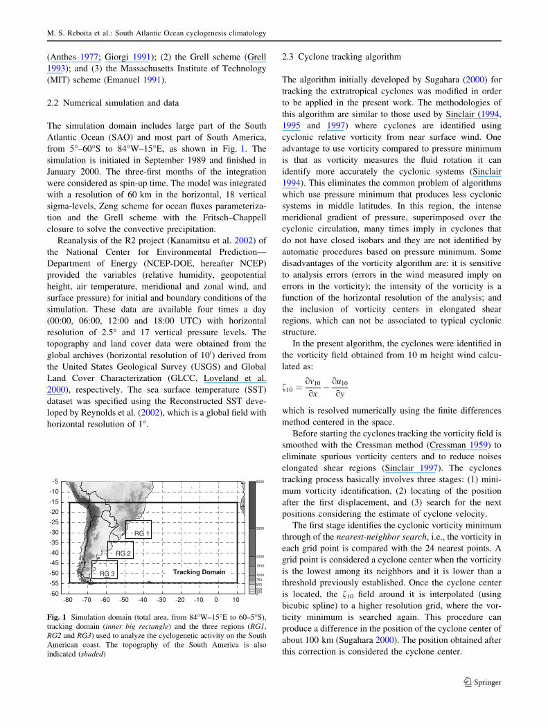
The simulation domain includes large part of the South

Atlantic Ocean (SAO) and most part of South America,

from 5�–60�S to 84�W–15�E, as shown in Fig. 1. The

simulation is initiated in September 1989 and finished in

January 2000. The three-first months of the integration

were considered as spin-up time. The model was integrated

with a resolution of 60 km in the horizontal, 18 vertical

sigma-levels, Zeng scheme for ocean fluxes parameteriza-

tion and the Grell scheme with the Fritsch–Chappell

closure to solve the convective precipitation.

Reanalysis of the R2 project (Kanamitsu et al. 2002) of

the National Center for Environmental Prediction—

Department of Energy (NCEP-DOE, hereafter NCEP)

provided the variables (relative humidity, geopotential

height, air temperature, meridional and zonal wind, and

surface pressure) for initial and boundary conditions of the

simulation. These data are available four times a day

(00:00, 06:00, 12:00 and 18:00 UTC) with horizontal

resolution of 2.5� and 17 vertical pressure levels. The

topography and land cover data were obtained from the

global archives (horizontal resolution of 100) derived from

the United States Geological Survey (USGS) and Global

Land Cover Characterization (GLCC, Loveland et al.

2000), respectively. The sea surface temperature (SST)

dataset was specified using the Reconstructed SST deve-

loped by Reynolds et al. (2002), which is a global field with

horizontal resolution of 1�.

2.3 Cyclone tracking algorithm

The algorithm initially developed by Sugahara (2000) for

tracking the extratropical cyclones was modified in order

to be applied in the present work. The methodologies of

this algorithm are similar to those used by Sinclair (1994,

1995 and 1997) where cyclones are identified using

cyclonic relative vorticity from near surface wind. One

advantage to use vorticity compared to pressure minimum

is that as vorticity measures the fluid rotation it can

identify more accurately the cyclonic systems (Sinclair

1994). This eliminates the common problem of algorithms

which use pressure minimum that produces less cyclonic

systems in middle latitudes. In this region, the intense

meridional gradient of pressure, superimposed over the

cyclonic circulation, many times imply in cyclones that

do not have closed isobars and they are not identified by

automatic procedures based on pressure minimum. Some

disadvantages of the vorticity algorithm are: it is sensitive

to analysis errors (errors in the wind measured imply on

errors in the vorticity); the intensity of the vorticity is a

function of the horizontal resolution of the analysis; and

the inclusion of vorticity centers in elongated shear

regions, which can not be associated to typical cyclonic

structure.

In the present algorithm, the cyclones were identified in

the vorticity field obtained from 10 m height wind calcu-

lated as:

f10 ¼ov10

ox� ou10

oy

which is resolved numerically using the finite differences

method centered in the space.

Before starting the cyclones tracking the vorticity field is

smoothed with the Cressman method (Cressman 1959) to

eliminate spurious vorticity centers and to reduce noises

elongated shear regions (Sinclair 1997). The cyclones

tracking process basically involves three stages: (1) mini-

mum vorticity identification, (2) locating of the position

after the first displacement, and (3) search for the next

positions considering the estimate of cyclone velocity.

The first stage identifies the cyclonic vorticity minimum

through of the nearest-neighbor search, i.e., the vorticity in

each grid point is compared with the 24 nearest points. A

grid point is considered a cyclone center when the vorticity

is the lowest among its neighbors and it is lower than a

threshold previously established. Once the cyclone center

is located, the f10 field around it is interpolated (using

bicubic spline) to a higher resolution grid, where the vor-

ticity minimum is searched again. This procedure can

produce a difference in the position of the cyclone center of

about 100 km (Sugahara 2000). The position obtained after

this correction is considered the cyclone center.

01002505007501000

1500

2000

3500

6000

-80 -70 -60 -50 -40 -30 -20 -10 0 10-60

-55

-50

-45

-40

-35

-30

-25

-20

-15

-10

-5

RG 1

RG 2

RG 3 Tracking Domain

Fig. 1 Simulation domain (total area, from 84�W–15�E to 60–5�S),

tracking domain (inner big rectangle) and the three regions (RG1,

RG2 and RG3) used to analyze the cyclogenetic activity on the South

American coast. The topography of the South America is also

indicated (shaded)

M. S. Reboita et al.: South Atlantic Ocean cyclogenesis climatology

123

A cyclone trajectory is defined as a sequence of its

position in the time {x(t), y(t)} and the system lifetime is

obtained from its first identification up to its disappearance.

After identify the cyclone first position (stage 1) is neces-

sary to identify its position after the first displacement

(stage 2) and the next positions (stage 3). As in Sinclair

(1994) the cyclone trajectory is performed to match

cyclones at the current time t with the centers obtained for

the following analysis time t ? Dt. In the stage 2, the

cyclone localization obtained in the stage 1 is used to

search the new cyclone center position by comparing with

the nearest-neighbor points, i.e., the first position is repe-

ated in the following time (t ? Dt) and there is a search by

vorticity minimum in the 24 grid points around. Once the

position of the system between two consecutive time

intervals is known the cyclone speed is calculated. This

velocity is used to estimate the new position in the next

time step (stage 3). After the identification of this probable

position of the system center, the algorithm searches again

the vorticity minimum in the 24 grid points around. Future

positions are determined considering the estimative of

cyclone velocity between the two consecutive time inter-

vals and cyclonic vorticity threshold. In the stages 2 and 3

the position of the cyclone center is also corrected in a high

resolution grid. The end of the cyclone occurs when both

the vorticity minimum and its lifetime overcome the

thresholds previously established.

At each time step the vorticity minima are considered as

new cyclone. This results in many trajectories for the same

system. After all tracking a filter is used to eliminate the

trajectories that have a minimum of three repeatedly

positions and times. Sometimes two systems starting in

different places can join, assuming similar positions during

part of their lifetime. If this happens, in order to not allow

the filter to eliminate the last system it is necessary to

verify if it has at least five different positions before. In this

case the second system is not eliminated by filter.

The final result of the algorithm supplies the cyclone

center position (latitude and longitude), date, pressure and

its f10.

2.4 Analysis methods

The 10-m height wind field with 6-h-temporal resolution

obtained from the NCEP and the RegCM3 are originally

in a gaussian grid and Mercator projection, respectively.

For the cyclones tracking, the bi-linear interpolation

scheme was used to construct a 2.5� 9 2.5� regular grid.

The objective was to guarantee that we are seeking the

same type of system in the RegCM3 and in the NCEP. It

is known that vorticity is very dependent of the grid

resolution; however, the frequency and intensity of the

cyclones are also sensitive to that (Pinto et al. 2006).

Adopting the same low resolution grid is a procedure that

filters small scale cyclogenesis of the RegCM3 higher

resolution and also does not create unrealistic cyclones

that could result from the interpolation of NCEP to

RegCM3 grid.

The tracking algorithm compares the vorticity values

with the 24 nearest grid points. The adopted thresholds for

cyclone identification were: (a) f10 B -1.5 9 10-5 s-1,

(b) T C 24 h, where T is the cyclone lifetime; (c)

T B 10 days. The period of study is from January 1, 1990

to December 31, 1999. The cyclones tracking area is shown

in Fig. 1 and in the analyses of the results it was only

considered the systems that initiated over SAO. It is

important to mention that the methodology used identifies

vorticity minima associated with isobars open or closed.

A validation of the tracking algorithm was done by

comparing the vorticity fields (simulated and reanalysis)

and cyclone centers identified by the algorithm for several

months. It was found that the algorithm correctly tracks

most of the relative vorticity minima, i. e., the algorithm is

able to capture between 85 and 95% of the systems iden-

tified in the vorticity field.

The occurrence of cyclogenesis in the NCEP and Reg-

CM3 was investigated through annual, seasonal and

monthly means in the analysis domain (Fig. 1) and in three

subdomains shown in the Fig. 1 (RG1, RG2 and RG3).

These areas were chosen due the higher frequency of

cyclogenesis over the east coast of South America (Necco

1982a, b; Satyamurty et al. 1990; Gan and Rao 1991;

Sinclair 1996; Hoskins and Hodges 2005, and Reboita et al.

2005) and represent the south/southeastern coast of Brazil

(RG1), the La Plata River discharge in Uruguay (RG2) and

southeastern coast of Argentina (RG3). The cyclogenesis

geographical distribution was analyzed by calculating the

mean density that is the number of systems in a 5o 9 5�region divided by the same area. This procedure follows

Murray and Simmonds (1991) and to facility the results

presentation the mean density was multiplied by 104 in the

figures.

3 Results: cyclogenesis climatology

3.1 Subjective comparison: NCEP 9 RegCM3

The comparison between the cyclones obtained from the

NCEP and those simulated by the RegCM3 shows that the

later has a tendency to start 12–24 h after those NCEP.

However, in general the simulated systems tend to decay

after the observed ones. Therefore this implies in a similar

cyclone lifetime for the NCEP and RegCM3.

Cyclogeneses monthly frequency over SAO, in general,

shows a little difference between NCEP and RegCM3.

M. S. Reboita et al.: South Atlantic Ocean cyclogenesis climatology

123

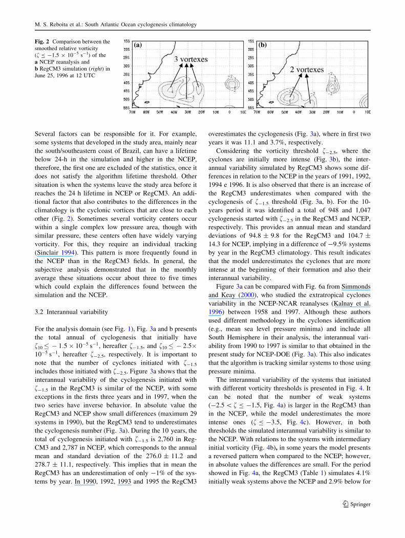
Several factors can be responsible for it. For example,

some systems that developed in the study area, mainly near

the south/southeastern coast of Brazil, can have a lifetime

below 24-h in the simulation and higher in the NCEP,

therefore, the first one are excluded of the statistics, once it

does not satisfy the algorithm lifetime threshold. Other

situation is when the systems leave the study area before it

reaches the 24 h lifetime in NCEP or RegCM3. An addi-

tional factor that also contributes to the differences in the

climatology is the cyclonic vortices that are close to each

other (Fig. 2). Sometimes several vorticity centers occur

within a single complex low pressure area, though with

similar pressure, these centers often have widely varying

vorticity. For this, they require an individual tracking

(Sinclair 1994). This pattern is more frequently found in

the NCEP than in the RegCM3 fields. In general, the

subjective analysis demonstrated that in the monthly

average these situations occur about three to five times

which could explain the differences found between the

simulation and the NCEP.

3.2 Interannual variability

For the analysis domain (see Fig. 1), Fig. 3a and b presents

the total annual of cyclogenesis that initially have

f10� � 1:5� 10�5 s�1, hereafter f-1.5, and f10� � 2:5�10�5 s�1, hereafter f-2.5, respectively. It is important to

note that the number of cyclones initiated with f-1.5

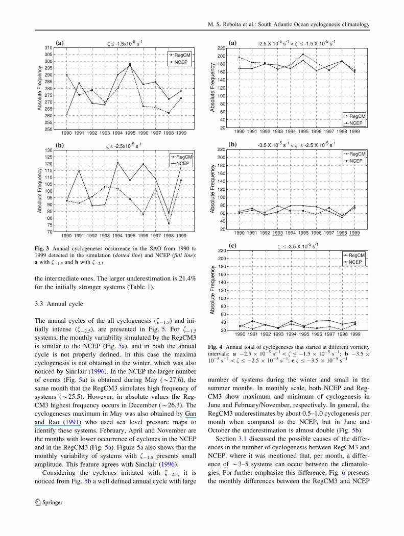
includes those initiated with f-2.5. Figure 3a shows that the

interannual variability of the cyclogenesis initiated with

f-1.5 in the RegCM3 is similar of the NCEP, with some

exceptions in the firsts three years and in 1997, when the

two series have inverse behavior. In absolute value the

RegCM3 and NCEP show small differences (maximum 29

systems in 1990), but the RegCM3 tend to underestimates

the cyclogenesis number (Fig. 3a). During the 10 years, the

total of cyclogenesis initiated with f-1.5 is 2,760 in Reg-

CM3 and 2,787 in NCEP, which corresponds to the annual

mean and standard deviation of the 276.0 ± 11.2 and

278.7 ± 11.1, respectively. This implies that in mean the

RegCM3 has an underestimation of only -1% of the sys-

tems by year. In 1990, 1992, 1993 and 1995 the RegCM3

overestimates the cyclogenesis (Fig. 3a), where in first two

years it was 11.1 and 3.7%, respectively.

Considering the vorticity threshold f-2.5, where the

cyclones are initially more intense (Fig. 3b), the inter-

annual variability simulated by RegCM3 shows some dif-

ferences in relation to the NCEP in the years of 1991, 1992,

1994 e 1996. It is also observed that there is an increase of

the RegCM3 underestimates when compared with the

cyclogenesis of f-1.5 threshold (Fig. 3a, b). For the 10-

years period it was identified a total of 948 and 1,047

cyclogenesis started with f-2.5 in the RegCM3 and NCEP,

respectively. This provides an annual mean and standard

deviations of 94.8 ± 9.8 for the RegCM3 and 104.7 ±

14.3 for NCEP, implying in a difference of -9.5% systems

by year in the RegCM3 climatology. This result indicates

that the model underestimates the cyclones that are more

intense at the beginning of their formation and also their

interannual variability.

Figure 3a can be compared with Fig. 6a from Simmonds

and Keay (2000), who studied the extratropical cyclones

variability in the NCEP-NCAR reanalyses (Kalnay et al.

1996) between 1958 and 1997. Although these authors

used different methodology in the cyclones identification

(e.g., mean sea level pressure minima) and include all

South Hemisphere in their analysis, the interannual vari-

ability from 1990 to 1997 is similar to that obtained in the

present study for NCEP-DOE (Fig. 3a). This also indicates

that the algorithm is tracking similar systems to those using

pressure minima.

The interannual variability of the systems that initiated

with different vorticity thresholds is presented in Fig. 4. It

can be noted that the number of weak systems

(-2.5 \ f B -1.5, Fig. 4a) is larger in the RegCM3 than

in the NCEP, while the model underestimates the more

intense ones (f B -3.5, Fig. 4c). However, in both

thresholds the simulated interannual variability is similar to

the NCEP. With relations to the systems with intermediary

initial vorticity (Fig. 4b), in some years the model presents

a reversed pattern when compared to the NCEP; however,

in absolute values the differences are small. For the period

showed in Fig. 4a, the RegCM3 (Table 1) simulates 4.1%

initially weak systems above the NCEP and 2.9% below for

Fig. 2 Comparison between the

smoothed relative vorticity

(f B -1.5 9 10-5 s-1) of the

a NCEP reanalysis and

b RegCM3 simulation (right) in

June 25, 1996 at 12 UTC

M. S. Reboita et al.: South Atlantic Ocean cyclogenesis climatology

123

the intermediate ones. The larger underestimation is 21.4%

for the initially stronger systems (Table 1).

3.3 Annual cycle

The annual cycles of the all cyclogenesis (f-1.5) and ini-

tially intense (f-2.5), are presented in Fig. 5. For f-1.5

systems, the monthly variability simulated by the RegCM3

is similar to the NCEP (Fig. 5a), and in both the annual

cycle is not properly defined. In this case the maxima

cyclogenesis is not obtained in the winter, which was also

noticed by Sinclair (1996). In the NCEP the larger number

of events (Fig. 5a) is obtained during May (*27.6), the

same month that the RegCM3 simulates high frequency of

systems (*25.5). However, in absolute values the Reg-

CM3 highest frequency occurs in December (*26.3). The

cyclogeneses maximum in May was also obtained by Gan

and Rao (1991) who used sea level pressure maps to

identify these systems. February, April and November are

the months with lower occurrence of cyclones in the NCEP

and in the RegCM3 (Fig. 5a). Figure 5a also shows that the

monthly variability of systems with f-1.5 presents small

amplitude. This feature agrees with Sinclair (1996).

Considering the cyclones initiated with f-2.5, it is

noticed from Fig. 5b a well defined annual cycle with large

number of systems during the winter and small in the

summer months. In monthly scale, both NCEP and Reg-

CM3 show maximum and minimum of cyclogenesis in

June and February/November, respectively. In general, the

RegCM3 underestimates by about 0.5–1.0 cyclogenesis per

month when compared to the NCEP, but in June and

October the underestimation is almost double (Fig. 5b).

Section 3.1 discussed the possible causes of the differ-

ences in the number of cyclogenesis between RegCM3 and

NCEP, where it was mentioned that, per month, a differ-

ence of *3–5 systems can occur between the climatolo-

gies. For further emphasize this difference, Fig. 6 presents

the monthly differences between the RegCM3 and NCEP

1990 1991 1992 1993 1994 1995 1996 1997 1998 1999250

255

260

265

270

275

280

285

290

295

300

305

310

Abs

olut

e F

requ

ency

-1.5x10-5 s-1

RegCM

NCEP

1990 1991 1992 1993 1994 1995 1996 1997 1998 199970

75

80

85

90

95

100

105

110

115

120

125

130

Abs

olut

e F

requ

ency

-2.5x10-5 s-1

RegCMNCEP

(a)

(b)

Fig. 3 Annual cyclogeneses occurrence in the SAO from 1990 to

1999 detected in the simulation (dotted line) and NCEP (full line):

a with f-1.5 and b with f-2.5

1990 1991 1992 1993 1994 1995 1996 1997 1998 199920

40

60

80

100

120

140

160

180

200

220

Abs

olut

e F

requ

ency

-2.5 X 10-5 s-1 < -1.5 X 10-5 s-1

RegCM

NCEP

1990 1991 1992 1993 1994 1995 1996 1997 1998 199920

40

60

80

100

120

140

160

180

200

220

Abs

olut

e F

requ

ency

-3.5 X 10-5 s-1 < -2.5 X 10-5 s-1

RegCM

NCEP

1990 1991 1992 1993 1994 1995 1996 1997 1998 199920

40

60

80

100

120

140

160

180

200

220

Abs

olut

e F

requ

ency

-3.5 X 10-5 s-1

RegCM

NCEP

(a)

(b)

(c)

Fig. 4 Annual total of cyclogeneses that started at different vorticity

intervals: a -2.5 9 10-5 s-1 \ f B -1.5 9 10-5 s-1; b -3.5 9

10-5 s-1 \ f B -2.5 9 10-5 s-1; c f B -3.5 9 10-5 s-1

M. S. Reboita et al.: South Atlantic Ocean cyclogenesis climatology

123

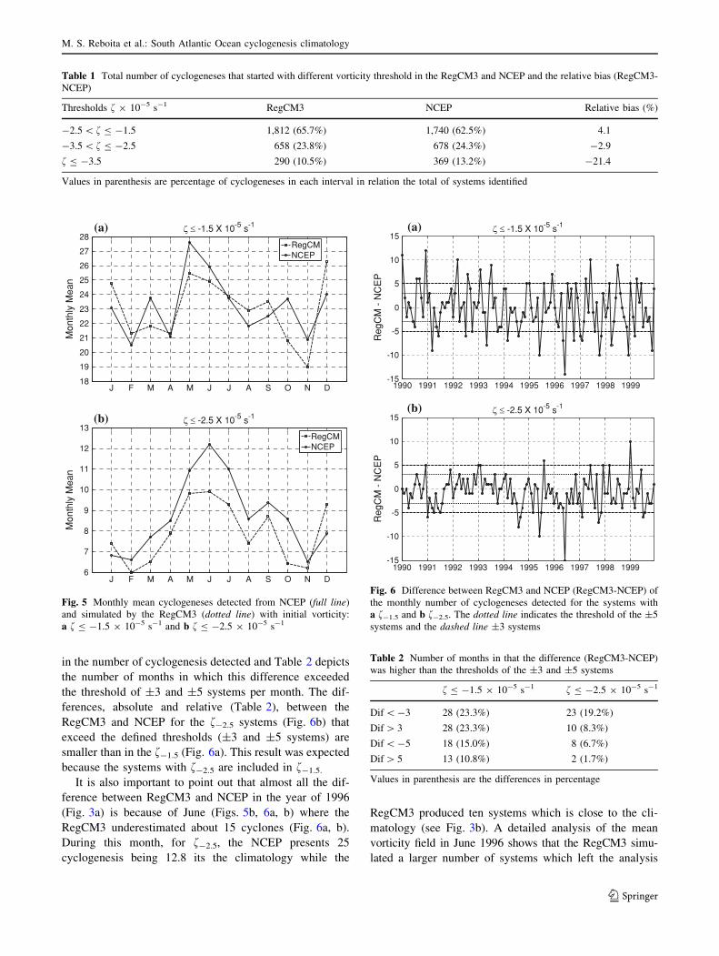
in the number of cyclogenesis detected and Table 2 depicts

the number of months in which this difference exceeded

the threshold of ±3 and ±5 systems per month. The dif-

ferences, absolute and relative (Table 2), between the

RegCM3 and NCEP for the f-2.5 systems (Fig. 6b) that

exceed the defined thresholds (±3 and ±5 systems) are

smaller than in the f-1.5 (Fig. 6a). This result was expected

because the systems with f-2.5 are included in f-1.5.

It is also important to point out that almost all the dif-

ference between RegCM3 and NCEP in the year of 1996

(Fig. 3a) is because of June (Figs. 5b, 6a, b) where the

RegCM3 underestimated about 15 cyclones (Fig. 6a, b).

During this month, for f-2.5, the NCEP presents 25

cyclogenesis being 12.8 its the climatology while the

RegCM3 produced ten systems which is close to the cli-

matology (see Fig. 3b). A detailed analysis of the mean

vorticity field in June 1996 shows that the RegCM3 simu-

lated a larger number of systems which left the analysis

Table 1 Total number of cyclogeneses that started with different vorticity threshold in the RegCM3 and NCEP and the relative bias (RegCM3-

NCEP)

Thresholds f 9 10-5 s-1 RegCM3 NCEP Relative bias (%)

-2.5 \ f B -1.5 1,812 (65.7%) 1,740 (62.5%) 4.1

-3.5 \ f B -2.5 658 (23.8%) 678 (24.3%) -2.9

f B -3.5 290 (10.5%) 369 (13.2%) -21.4

Values in parenthesis are percentage of cyclogeneses in each interval in relation the total of systems identified

J F M A M J J A S O N D18

19

20

21

22

23

24

25

26

27

28

Mon

thly

Mea

n

-1.5 X 10-5 s-1

RegCMNCEP

J F M A M J J A S O N D6

7

8

9

10

11

12

13

Mon

thly

Mea

n

-2.5 X 10-5 s-1

RegCMNCEP

(a)

(b)

Fig. 5 Monthly mean cyclogeneses detected from NCEP (full line)

and simulated by the RegCM3 (dotted line) with initial vorticity:

a f B -1.5 9 10-5 s-1 and b f B -2.5 9 10-5 s-1

1990 1991 1992 1993 1994 1995 1996 1997 1998 1999-15

-10

-5

0

5

10

15

Reg

CM

- N

CE

P

-1.5 X 10-5 s-1

1990 1991 1992 1993 1994 1995 1996 1997 1998 1999-15

-10

-5

0

5

10

15 -2.5 X 10-5 s-1

Reg

CM

- N

CE

P

(a)

(b)

Fig. 6 Difference between RegCM3 and NCEP (RegCM3-NCEP) of

the monthly number of cyclogeneses detected for the systems with

a f-1.5 and b f-2.5. The dotted line indicates the threshold of the ±5

systems and the dashed line ±3 systems

Table 2 Number of months in that the difference (RegCM3-NCEP)

was higher than the thresholds of the ±3 and ±5 systems

f B -1.5 9 10-5 s-1 f B -2.5 9 10-5 s-1

Dif \ -3 28 (23.3%) 23 (19.2%)

Dif [ 3 28 (23.3%) 10 (8.3%)

Dif \ -5 18 (15.0%) 8 (6.7%)

Dif [ 5 13 (10.8%) 2 (1.7%)

Values in parenthesis are the differences in percentage

M. S. Reboita et al.: South Atlantic Ocean cyclogenesis climatology

123

region before they completed 24 h and, therefore they were

not counted. Also, the RegCM3 presented lower number of

multiple cyclonic vortices (similar to Fig. 2) than NCEP in

this month.

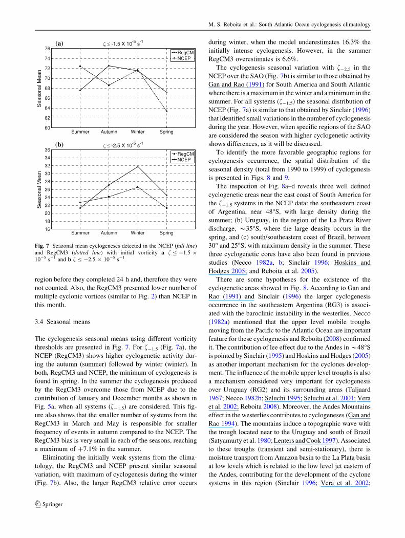
3.4 Seasonal means

The cyclogenesis seasonal means using different vorticity

thresholds are presented in Fig. 7. For f-1.5 (Fig. 7a), the

NCEP (RegCM3) shows higher cyclogenetic activity dur-

ing the autumn (summer) followed by winter (winter). In

both, RegCM3 and NCEP, the minimum of cyclogenesis is

found in spring. In the summer the cyclogenesis produced

by the RegCM3 overcome those from NCEP due to the

contribution of January and December months as shown in

Fig. 5a, when all systems (f-1.5) are considered. This fig-

ure also shows that the smaller number of systems from the

RegCM3 in March and May is responsible for smaller

frequency of events in autumn compared to the NCEP. The

RegCM3 bias is very small in each of the seasons, reaching

a maximum of ?7.1% in the summer.

Eliminating the initially weak systems from the clima-

tology, the RegCM3 and NCEP present similar seasonal

variation, with maximum of cyclogenesis during the winter

(Fig. 7b). Also, the larger RegCM3 relative error occurs

during winter, when the model underestimates 16.3% the

initially intense cyclogenesis. However, in the summer

RegCM3 overestimates is 6.6%.

The cyclogenesis seasonal variation with f-2.5 in the

NCEP over the SAO (Fig. 7b) is similar to those obtained by

Gan and Rao (1991) for South America and South Atlantic

where there is a maximum in the winter and a minimum in the

summer. For all systems (f-1.5) the seasonal distribution of

NCEP (Fig. 7a) is similar to that obtained by Sinclair (1996)

that identified small variations in the number of cyclogenesis

during the year. However, when specific regions of the SAO

are considered the season with higher cyclogenetic activity

shows differences, as it will be discussed.

To identify the more favorable geographic regions for

cyclogenesis occurrence, the spatial distribution of the

seasonal density (total from 1990 to 1999) of cyclogenesis

is presented in Figs. 8 and 9.

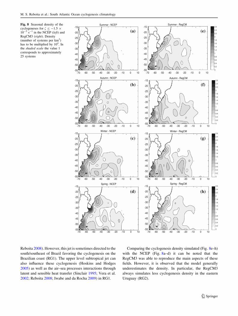
The inspection of Fig. 8a–d reveals three well defined

cyclogenetic areas near the east coast of South America for

the f-1.5 systems in the NCEP data: the southeastern coast

of Argentina, near 48�S, with large density during the

summer; (b) Uruguay, in the region of the La Prata River

discharge, *35�S, where the large density occurs in the

spring, and (c) south/southeastern coast of Brazil, between

30� and 25�S, with maximum density in the summer. These

three cyclogenetic cores have also been found in previous

studies (Necco 1982a, b; Sinclair 1996; Hoskins and

Hodges 2005; and Reboita et al. 2005).

There are some hypotheses for the existence of the

cyclogenetic areas showed in Fig. 8. According to Gan and

Rao (1991) and Sinclair (1996) the larger cyclogenesis

occurrence in the southeastern Argentina (RG3) is associ-

ated with the baroclinic instability in the westerlies. Necco

(1982a) mentioned that the upper level mobile troughs

moving from the Pacific to the Atlantic Ocean are important

feature for these cyclogenesis and Reboita (2008) confirmed

it. The contribution of lee effect due to the Andes in *48�S

is pointed by Sinclair (1995) and Hoskins and Hodges (2005)

as another important mechanism for the cyclones develop-

ment. The influence of the mobile upper level troughs is also

a mechanism considered very important for cyclogenesis

over Uruguay (RG2) and its surrounding areas (Taljaard

1967; Necco 1982b; Seluchi 1995; Seluchi et al. 2001; Vera

et al. 2002; Reboita 2008). Moreover, the Andes Mountains

effect in the westerlies contributes to cyclogeneses (Gan and

Rao 1994). The mountains induce a topographic wave with

the trough located near to the Uruguay and south of Brazil

(Satyamurty et al. 1980; Lenters and Cook 1997). Associated

to these troughs (transient and semi-stationary), there is

moisture transport from Amazon basin to the La Plata basin

at low levels which is related to the low level jet eastern of

the Andes, contributing for the development of the cyclone

systems in this region (Sinclair 1996; Vera et al. 2002;

(a)

(b)

Summer Autumn Winter Spring60

62

64

66

68

70

72

74

76

Sea

sona

l Mea

n -1.5 X 10-5 s-1

RegCMNCEP

Summer Autumn Winter Spring16

18

20

22

24

26

28

30

32

34

36

Sea

sona

l Mea

n

-2.5 X 10-5 s-1

RegCMNCEP

Fig. 7 Seazonal mean cyclogeneses detected in the NCEP (full line)

and RegCM3 (dotted line) with initial vorticity a f B -1.5 9

10-5 s-1 and b f B -2.5 9 10-5 s-1

M. S. Reboita et al.: South Atlantic Ocean cyclogenesis climatology

123

Reboita 2008). However, this jet is sometimes directed to the

south/southeast of Brazil favoring the cyclogenesis on the

Brazilian coast (RG1). The upper level subtropical jet can

also influence these cyclogenesis (Hoskins and Hodges

2005) as well as the air–sea processes interactions through

latent and sensible heat transfer (Sinclair 1995; Vera et al.

2002; Reboita 2008; Iwabe and da Rocha 2009) in RG1.

Comparing the cyclogenesis density simulated (Fig. 8e–h)

with the NCEP (Fig. 8a–d) it can be noted that the

RegCM3 was able to reproduce the main aspects of these

fields. However, it is observed that the model generally

underestimates the density. In particular, the RegCM3

always simulates less cyclogenesis density in the eastern

Uruguay (RG2).

-70 -60 -50 -40 -30 -20 -10 0 10-55

-50

-45

-40

-35

-30

-25

-20

-15Summer - NCEP

-70 -60 -50 -40 -30 -20 -10 0 10-55

-50

-45

-40

-35

-30

-25

-20

-15Autumn - NCEP

-70 -60 -50 -40 -30 -20 -10 0 10-55

-50

-45

-40

-35

-30

-25

-20

-15Winter - NCEP

-70 -60 -50 -40 -30 -20 -10 0 10-55

-50

-45

-40

-35

-30

-25

-20

-15Spring - NCEP

0

0.2

0.4

0.6

0.8

1

1.2

1.4

1.6

1.8

2

2.2

2.4

2.6

-70 -60 -50 -40 -30 -20 -10 0 10-55

-50

-45

-40

-35

-30

-25

-20

-15Autumn - RegCM

0

0.2

0.4

0.6

0.8

1

1.2

1.4

1.6

1.8

2

2.2

2.4

2.6

-70 -60 -50 -40 -30 -20 -10 0 10-55

-50

-45

-40

-35

-30

-25

-20

-15Winter - RegCM

0

0.2

0.4

0.6

0.8

1

1.2

1.4

1.6

1.8

2

2.2

2.4

2.6

-70 -60 -50 -40 -30 -20 -10 0 10-55

-50

-45

-40

-35

-30

-25

-20

-15Spring - RegCM

0

0.2

0.4

0.6

0.8

1

1.2

1.4

1.6

1.8

2

2.2

2.4

2.6

-70 -60 -50 -40 -30 -20 -10 0 10-55

-50

-45

-40

-35

-30

-25

-20

-15Summer - RegCM

(a)

(b)

(c)

(d)

(e)

(f)

(g)

(h)

Fig. 8 Seasonal density of the

cyclogeneses for f B -1.5 9

10-5 s-1 in the NCEP (left) and

RegCM3 (right). Density

(number of systems per km2)

has to be multiplied by 104. In

the shaded scale the value 1

corresponds to approximately

25 systems

M. S. Reboita et al.: South Atlantic Ocean cyclogenesis climatology

123

Similar to the NCEP (Fig. 8a), the RegCM3 (Fig. 8e)

also shows larger cyclogenesis density over the south/

southeastern coast of Brazil (RG1) during the summer, but

it underestimates the density and its core maximum is

displaced toward southwestern (Fig. 8a–e). However, dur-

ing the winter (Fig. 8c–g) and spring (Fig. 8d–h) the

simulated density is similar to the NCEP. In the Uruguay

coast (RG2), the RegCM3 does not reproduce the density

maximum presents in the NCEP during the summer

(Fig. 8a–e) and autumn (Fig. 8b–f), but it simulates a

weaker maximum in the winter (Fig. 8c–g) and spring

(Fig. 8d–h).

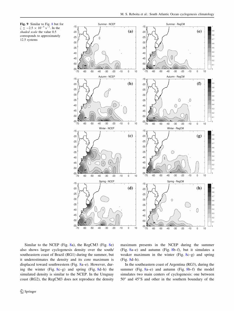
In the southeastern coast of Argentina (RG3), during the

summer (Fig. 8a–e) and autumn (Fig. 8b–f) the model

simulates two main centers of cyclogenesis: one between

50� and 45�S and other in the southern boundary of the

-70 -60 -50 -40 -30 -20 -10 0 10-55

-50

-45

-40

-35

-30

-25

-20

-15Summer - NCEP

-70 -60 -50 -40 -30 -20 -10 0 10-55

-50

-45

-40

-35

-30

-25

-20

-15Winter - NCEP

-70 -60 -50 -40 -30 -20 -10 0 10-55

-50

-45

-40

-35

-30

-25

-20

-15Autumn - NCEP

-70 -60 -50 -40 -30 -20 -10 0 10-55

-50

-45

-40

-35

-30

-25

-20

-15Spring - NCEP

0

0.1

0.2

0.3

0.4

0.5

0.6

0.7

0.8

0.9

1

-70 -60 -50 -40 -30 -20 -10 0 10-55

-50

-45

-40

-35

-30

-25

-20

-15Summer - RegCM

0

0.1

0.2

0.3

0.4

0.5

0.6

0.7

0.8

0.9

1

-70 -60 -50 -40 -30 -20 -10 0 10-55

-50

-45

-40

-35

-30

-25

-20

-15Autumn - RegCM

0

0.1

0.2

0.3

0.4

0.5

0.6

0.7

0.8

0.9

1

-70 -60 -50 -40 -30 -20 -10 0 10-55

-50

-45

-40

-35

-30

-25

-20

-15Spring - RegCM

0

0.1

0.2

0.3

0.4

0.5

0.6

0.7

0.8

0.9

1

-70 -60 -50 -40 -30 -20 -10 0 10-55

-50

-45

-40

-35

-30

-25

-20

-15Winter - RegCM

(a)

(b)

(c)

(d)

(e)

(f)

(g)

(h)

Fig. 9 Similar to Fig. 8 but for

f B -2.5 9 10-5 s-1. In the

shaded scale the value 0.5

corresponds to approximately

12.5 systems

M. S. Reboita et al.: South Atlantic Ocean cyclogenesis climatology

123

domain (55�S). This result differs from the NCEP which

only shows a core that oscillates between 45�S (summer)

and 50�S (autumn). During the winter (Fig. 8c–g), the

RegCM3 reproduces the intensity and location of the

cyclogenetic core obtained in the NCEP. In the RG3,

the model underestimates the cyclogenesis density in the

spring (Fig. 8d–h). The simulated cyclogenesis maximum

density in the RG3 occurs in the autumn and winter, dif-

fering from the NCEP where the maximum is only in the

summer.

When only the f-2.5 systems are considered, there is a

clear reduction of the cyclogenetic density in the south/

southeastern Brazilian coast for the NCEP and RegCM3

(Fig. 9). This reduces the number of cyclogeneses areas

near the east coast of South America to two and the larger

cyclogenetic activity occurs in the winter (Fig. 9c–g).

Close to the La Prata River discharge (RG2) the NCEP

shows intense cyclonegesis during all seasons with higher

density during the spring (Fig. 9d). However, similar to

Fig. 8, the area occupied is larger in the winter (Fig. 9c)

which may explain the larger number of cyclogenesis in

this season (Fig. 7b) when the cyclogenetic density is

integrated over all RG2. On the other hand, the RegCM3

shows reduced cyclogenetic activity in the coast of Uru-

guay being displaced southward during the summer

(Fig. 9a, b) and spring (Fig. 9d–h). The simulated cyclo-

genetic density area over southeastern Argentina (RG3) is

also displaced southward, except in the winter (Fig. 9c–g),

where the cyclogenetic cores are similar in position to the

NCEP.

3.5 The three cyclogenetic regions: seasonal variability

Figures 8 and 9 clearly show that there are three regions

where the cyclogenesis is more frequent in the east coast of

South America. However, the density of the cyclogenesis is

dependent of the region and season. In order to investigate

theses questions three subdomains (RG1, RG2 and RG3)

were established as shown in Fig. 1.

The total number of systems from 1990 to 1999 in the

RG1, RG2 and RG3 are presented in Table 3. In general,

the total number of systems in each area is larger in the

NCEP than RegCM3. Concerning the cyclogenesis initi-

ated with f-1.5, the larger RegCM3 underestimation is

obtained in the RG1 (-24%), while the better agreement

between RegCM3 and NCEP occurs in the RG3 (-6%).

For the initially more intense systems the RegCM3 was

less skilful in the RG2, where there is a negative relative

bias of -47%. In the RG1 as well as in the RG3 the

numbers of the initially more intense cyclogenesis simu-

lated are very similar to the NCEP.

As will be discussed in the Sect. 3.6, the RegCM3

simulated systems are weaker than in the NCEP. This

implied that in many simulated systems the vorticity

threshold (f-1.5) to tracking is not reached, being more

common in RG1 and RG2. In these regions, a reason for

the RegCM3 cyclogenesis underestimation is that the

simulated mid-high levels transient troughs (which cross

the South America from Pacific Ocean at subtropical lati-

tudes) are weaker than in the NCEP. Other feature that

contributes for weaker systems in model is that RegCM3

underestimation of the low-level moisture transport from

tropics to subtropics (Fernandez et al. 2006; Reboita 2008).

As previously presented in the literature, mid-high levels

trough (Seluchi 1995; Vera et al. 2002; Reboita 2008) and

moisture availablity (Vera et al. 2002; Reboita 2008) are

important mechanisms for cyclone development in the

RG1 and RG2. In the RG3 the RegCM3 simulates better

the mid-high levels trough amplitude, explaining the better

agreement between RegCM3 and NCEP cyclones

climatology.

The rate between initially intense and all systems

simulated by RegCM3 is similar to that obtained with the

NCEP (Table 3), except for the RG2 where it is almost half

of the NCEP. In RG1, the RegCM3 and NCEP indicate

predominance of initially weak cyclones, and the initially

more intense events represents 14 and 12%, respectively,

of the total cyclogenesis.

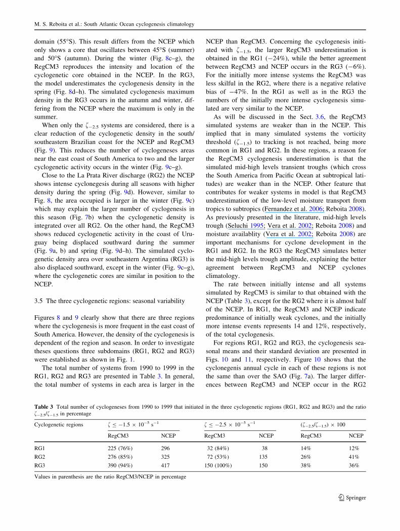
For regions RG1, RG2 and RG3, the cyclogenesis sea-

sonal means and their standard deviation are presented in

Figs. 10 and 11, respectively. Figure 10 shows that the

cyclonegenis annual cycle in each of these regions is not

the same than over the SAO (Fig. 7a). The larger differ-

ences between RegCM3 and NCEP occur in the RG2

Table 3 Total number of cyclogeneses from 1990 to 1999 that initiated in the three cyclogenetic regions (RG1, RG2 and RG3) and the ratio

f-2.5/f-1.5 in percentage

Cyclogenetic regions f B -1.5 9 10-5 s-1 f B -2.5 9 10-5 s-1 (f-2.5/f-1.5) 9 100

RegCM3 NCEP RegCM3 NCEP RegCM3 NCEP

RG1 225 (76%) 296 32 (84%) 38 14% 12%

RG2 276 (85%) 325 72 (53%) 135 26% 41%

RG3 390 (94%) 417 150 (100%) 150 38% 36%

Values in parenthesis are the ratio RegCM3/NCEP in percentage

M. S. Reboita et al.: South Atlantic Ocean cyclogenesis climatology

123

(Fig. 10b–e). In this area, the RegCM3 (Fig. 10b–e) sim-

ulates an almost uniform distribution of the cyclogenesis

during the year while the NCEP (Fig. 10b–e) shows a peak

in the winter. For the RG1 (Fig. 10a) NCEP and RegCM3

present larger frequency of f-1.5 during the summer and

suffer a reduction in the autumn, and the RegCM3 in

general underestimates the NCEP. In this same area, the

f-2.5 are well distributed during the year (Fig. 10d) and

they represent a small fraction of the total (Fig. 10a–c). In

RG3 (Fig. 10c), except by the drastic reduction of the

simulated f-1.5 cyclonegenesis during the spring

(Fig. 10c), the RegCM3 annual cycle is similar to the

NCEP. For the more intense cyclogenesis (Fig. 10f) the

amplitude of annual cycle is larger and there is a peak in

the winter and a decrease in the summer.

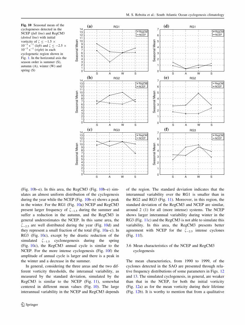
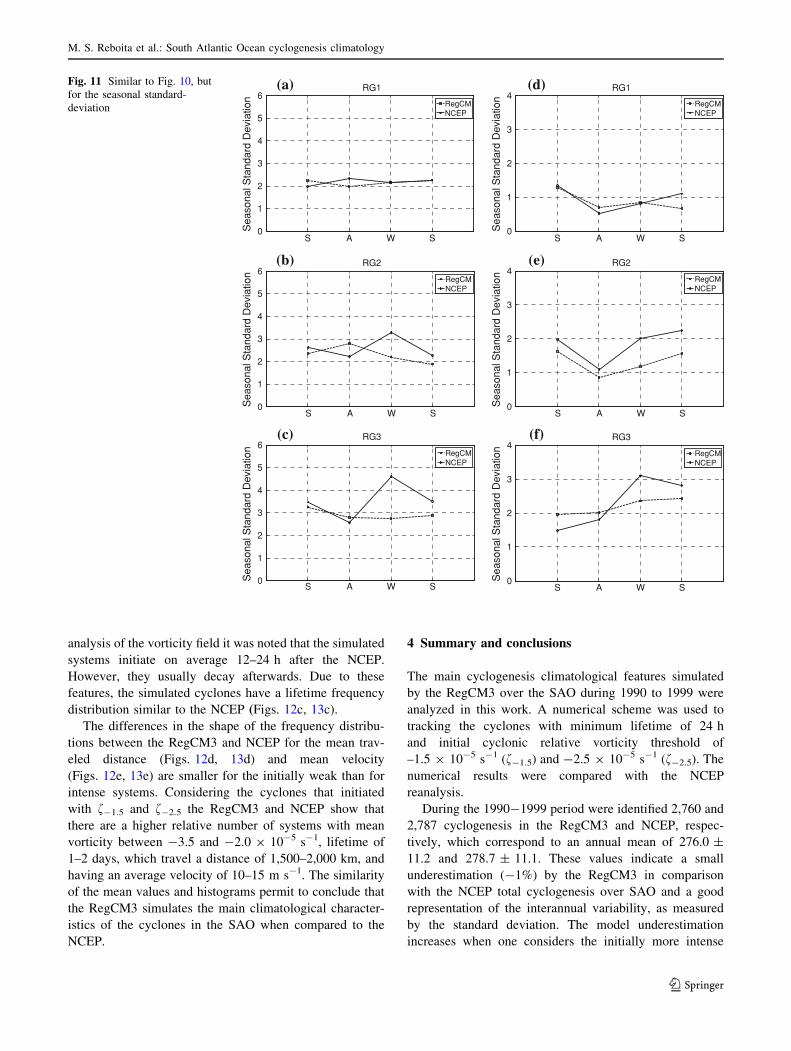
In general, considering the three areas and the two dif-

ferent vorticity thresholds, the interanual variability, as

measured by the standard deviation, simulated by the

RegCM3 is similar to the NCEP (Fig. 11), somewhat

centered in different mean values (Fig. 10). The large

interannual variability in the NCEP and RegCM3 depends

of the region. The standard deviation indicates that the

interannual variability over the RG1 is smaller than in

the RG2 and RG3 (Fig. 11). Moreover, in this region, the

standard deviation of the RegCM3 and NCEP are similar,

around 2 (1) for all (more intense) systems. The NCEP

shows larger interannual variability during winter in the

RG3 (Fig. 11c) and the RegCM3 is not able to simulate this

variability. In this area, the RegCM3 presents better

agreement with NCEP for the f-2.5 intense cyclones

(Fig. 11f).

3.6 Mean characteristics of the NCEP and RegCM3

cyclogenesis

The mean characteristics, from 1990 to 1999, of the

cyclones detected in the SAO are presented through rela-

tive frequency distributions of some parameters in Figs. 12

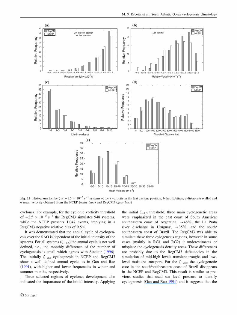
and 13. The simulated cyclogenesis, in general, are weaker

than that in the NCEP, for both the initial vorticity

(Fig. 12a) as for the mean vorticity during their lifetime

(Fig. 12b). It is worthy to mention that from a qualitative

S A W S0123456789

1011121314

Sea

sona

l Mea

n

RG1

RegCMNCEP

S A W S0123456789

1011121314

Sea

zona

l Mea

nRG2

S A W S0123456789

1011121314

Sea

sona

l Mea

n

RG3

S A W S0

1

2

3

4

5

6

7

Sea

sona

l Mea

n

RG1

S A W S0

1

2

3

4

5

6

7

Sea

sona

l Mea

n

RG2

S A W S0

1

2

3

4

5

6

7

Sea

sona

l Mea

n

RG3

RegCMNCEP

RegCMNCEP

RegCMNCEP

RegCMNCEP

RegCMNCEP

(a)

(b)

(c)

(d)

(e)

(f)

Fig. 10 Seasonal mean of the

cyclogeneses detected in the

NCEP (full line) and RegCM3

(dotted line) with initial

vorticity of f B -1.5 9

10-5 s-1 (left) and f B -2.5 9

10-5 s-1 (right) in each

cyclogenetic region shown in

Fig. 1. In the horizontal axis the

season order is summer (S),

autumn (A), winter (W) and

spring (S)

M. S. Reboita et al.: South Atlantic Ocean cyclogenesis climatology

123

analysis of the vorticity field it was noted that the simulated

systems initiate on average 12–24 h after the NCEP.

However, they usually decay afterwards. Due to these

features, the simulated cyclones have a lifetime frequency

distribution similar to the NCEP (Figs. 12c, 13c).

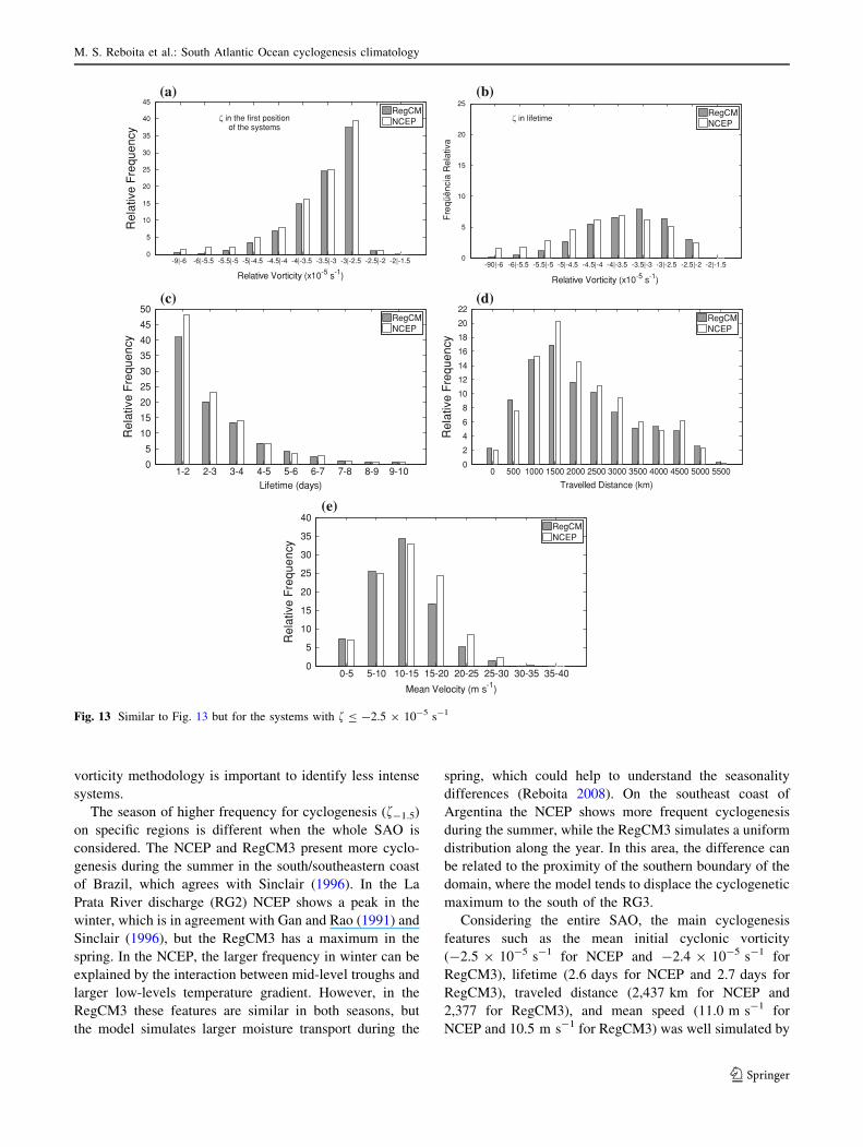
The differences in the shape of the frequency distribu-

tions between the RegCM3 and NCEP for the mean trav-

eled distance (Figs. 12d, 13d) and mean velocity

(Figs. 12e, 13e) are smaller for the initially weak than for

intense systems. Considering the cyclones that initiated

with f-1.5 and f-2.5 the RegCM3 and NCEP show that

there are a higher relative number of systems with mean

vorticity between -3.5 and -2.0 9 10-5 s-1, lifetime of

1–2 days, which travel a distance of 1,500–2,000 km, and

having an average velocity of 10–15 m s-1. The similarity

of the mean values and histograms permit to conclude that

the RegCM3 simulates the main climatological character-

istics of the cyclones in the SAO when compared to the

NCEP.

4 Summary and conclusions

The main cyclogenesis climatological features simulated

by the RegCM3 over the SAO during 1990 to 1999 were

analyzed in this work. A numerical scheme was used to

tracking the cyclones with minimum lifetime of 24 h

and initial cyclonic relative vorticity threshold of

–1.5 9 10-5 s-1 (f-1.5) and -2.5 9 10-5 s-1 (f-2.5). The

numerical results were compared with the NCEP

reanalysis.

During the 1990-1999 period were identified 2,760 and

2,787 cyclogenesis in the RegCM3 and NCEP, respec-

tively, which correspond to an annual mean of 276.0 ±

11.2 and 278.7 ± 11.1. These values indicate a small

underestimation (-1%) by the RegCM3 in comparison

with the NCEP total cyclogenesis over SAO and a good

representation of the interannual variability, as measured

by the standard deviation. The model underestimation

increases when one considers the initially more intense

S A W S0

1

2

3

4

5

6

Sea

sona

l Sta

ndar

d D

evia

tion

RG1

RegCMNCEP

S A W S0

1

2

3

4

5

6

Sea

sona

l Sta

ndar

d D

evia

tion

RG2

RegCMNCEP

S A W S0

1

2

3

4

5

6

Sea

sona

l Sta

ndar

d D

evia

tion

RG3

RegCMNCEP

S A W S0

1

2

3

4

Sea

sona

l Sta

ndar

d D

evia

tion

RG1

RegCMNCEP

S A W S0

1

2

3

4

Sea

sona

l Sta

ndar

d D

evia

tion

RG2

RegCMNCEP

S A W S0

1

2

3

4

Sea

sona

l Sta

ndar

d D

evia

tion

RG3

RegCMNCEP

(a)

(b)

(c)

(d)

(e)

(f)

Fig. 11 Similar to Fig. 10, but

for the seasonal standard-

deviation

M. S. Reboita et al.: South Atlantic Ocean cyclogenesis climatology

123

cyclones. For example, for the cyclonic vorticity threshold

of -2.5 9 10-5 s-1 the RegCM3 simulates 948 systems,

while the NCEP presents 1,047 events, implying in a

RegCM3 negative relative bias of 9.5%.

It was demonstrated that the annual cycle of cyclogen-

esis over the SAO is dependent of the initial intensity of the

systems. For all systems (f-1.5) the annual cycle is not well

defined, i.e., the monthly difference of the number of

cyclogenesis is small which agrees with Sinclair (1996).

The initially f-2.5 cyclogenesis in NCEP and RegCM3

show a well defined annual cycle, as in Gan and Rao

(1991), with higher and lower frequencies in winter and

summer months, respectively.

Three selected regions of cyclones development also

indicated the importance of the initial intensity. Applying

the initial f-1.5 threshold, three main cyclogenetic areas

were emphasized in the east coast of South America:

southeastern coast of Argentina, *48�S; the La Prata

river discharge in Uruguay, *35�S; and the south/

southeastern coast of Brazil. The RegCM3 was able to

simulate these three cylogenesis regions, however in some

cases (mainly in RG1 and RG2) it underestimates or

misplace the cyclogenesis density areas. These differences

are probably due to the RegCM3 deficiencies in the

simulation of mid-high levels transient troughs and low-

level moisture transport. For the f-2.5, the cyclogenetic

core in the south/southeastern coast of Brazil disappears

in the NCEP and RegCM3. This result is similar to pre-

vious studies that used sea level pressure to identify

cyclogenesis (Gan and Rao 1991) and it suggests that the

0 500 1000 1500 2000 2500 3000 3500 4000 4500 5000 55000

2

4

6

8

10

12

14

16

18

20

22

Travelled Distance (km)

Rel

ativ

e F

requ

ency

RegCMNCEP

1-2 2-3 3-4 4-5 5-6 6-7 7-8 8-9 9-100

5

10

15

20

25

30

35

40

45

50

Lifetime (days)

Rel

ativ

e F

requ

ency

0-5 5-10 10-15 15-20 20-25 25-30 30-35 35-400

5

10

15

20

25

30

35

40

Mean Velocity (m s-1)

Rel

ativ

e F

requ

ency

-9|-6 -6|-5.5 -5.5|-5 -5|-4.5 -4.5|-4 -4|-3.5 -3.5|-3 -3|-2.5 -2.5|-2 -2|-1.50

5

10

15

20

25

30

35

40

45

Relative Vorticity (x10-5s-1)

Rel

ativ

e F

requ

ency

-9|-6 -6|-5.5 -5.5|-5 -5|-4.5 -4.5|-4 -4|-3.5 -3.5|-3 -3|-2.5 -2.5|-2 -2|-1.50

5

10

15

20

25

Relative Vorticity (x10-5 s-1)

Rel

ativ

e Fr

eque

ncy

(a) (b)

(c) (d)

(e)

in the first position of the systems

in lifetime

RegCMNCEP

RegCMNCEP

RegCMNCEP

RegCMNCEP

Fig. 12 Histograms for the f B -1.5 9 10-5 s-1 systems of the a vorticity in the first cyclone position, b their lifetime, d distance travelled and

e mean velocity obtained from the NCEP (white bars) and RegCM3 (gray bars)

M. S. Reboita et al.: South Atlantic Ocean cyclogenesis climatology

123

vorticity methodology is important to identify less intense

systems.

The season of higher frequency for cyclogenesis (f-1.5)

on specific regions is different when the whole SAO is

considered. The NCEP and RegCM3 present more cyclo-

genesis during the summer in the south/southeastern coast

of Brazil, which agrees with Sinclair (1996). In the La

Prata River discharge (RG2) NCEP shows a peak in the

winter, which is in agreement with Gan and Rao (1991) and

Sinclair (1996), but the RegCM3 has a maximum in the

spring. In the NCEP, the larger frequency in winter can be

explained by the interaction between mid-level troughs and

larger low-levels temperature gradient. However, in the

RegCM3 these features are similar in both seasons, but

the model simulates larger moisture transport during the

spring, which could help to understand the seasonality

differences (Reboita 2008). On the southeast coast of

Argentina the NCEP shows more frequent cyclogenesis

during the summer, while the RegCM3 simulates a uniform

distribution along the year. In this area, the difference can

be related to the proximity of the southern boundary of the

domain, where the model tends to displace the cyclogenetic

maximum to the south of the RG3.

Considering the entire SAO, the main cyclogenesis

features such as the mean initial cyclonic vorticity

(-2.5 9 10-5 s-1 for NCEP and -2.4 9 10-5 s-1 for

RegCM3), lifetime (2.6 days for NCEP and 2.7 days for

RegCM3), traveled distance (2,437 km for NCEP and

2,377 for RegCM3), and mean speed (11.0 m s-1 for

NCEP and 10.5 m s-1 for RegCM3) was well simulated by

0 500 1000 1500 2000 2500 3000 3500 4000 4500 5000 55000

2

4

6

8

10

12

14

16

18

20

22

Travelled Distance (km)

Rel

ativ

e F

requ

ency

1-2 2-3 3-4 4-5 5-6 6-7 7-8 8-9 9-100

5

10

15

20

25

30

35

40

45

50

Lifetime (days)

Rel

ativ

e F

requ

ency

RegCMNCEP

0-5 5-10 10-15 15-20 20-25 25-30 30-35 35-400

5

10

15

20

25

30

35

40

Mean Velocity (m s-1)

Rel

ativ

e F

requ

ency

-9|-6 -6|-5.5 -5.5|-5 -5|-4.5 -4.5|-4 -4|-3.5 -3.5|-3 -3|-2.5 -2.5|-2 -2|-1.50

5

10

15

20

25

30

35

40

45

Relative Vorticity (x10-5 s-1)

Rel

ativ

e F

requ

ency

-90|-6 -6|-5.5 -5.5|-5 -5|-4.5 -4.5|-4 -4|-3.5 -3.5|-3 -3|-2.5 -2.5|-2 -2|-1.50

5

10

15

20

25

Relative Vorticity (x10-5 s-1)

Fre

qüên

cia

Rel

ativ

a

(a) (b)

(c) (d)

(e)

in the first position of the systems

in lifetime RegCMNCEP

RegCMNCEP

RegCMNCEP

RegCMNCEP

Fig. 13 Similar to Fig. 13 but for the systems with f B -2.5 9 10-5 s-1

M. S. Reboita et al.: South Atlantic Ocean cyclogenesis climatology

123

the RegCM3. These results indicate that the RegCM3 is

able to simulate the main features of the cyclogenesis cli-

matology on the SAO and it may be very useful to inves-

tigate many other properties of the cyclones development

in the region.

Acknowledgments The authors would like to thank FAPESP

(processes 04/02446-7 and 01/13925-5) and the CNPq (processes

475281/2003-9, 300348/2005-3, and 476361/2006-0) for financial

support. We also acknowledge the ICTP for providing the RegCM3

and NCEP for the reanalysis. CAPES has also provided partial sup-

port for this research.

References

Anthes RA (1977) A cumulus parameterization scheme utilizing a

one-dimensional cloud model. Mon Weather Rev 117:1423–

1438

Blender R, Fraedrich K, Lunkeit F (1997) Identification of cyclone-

track regimes in the North Atlantic. Q J R Meteorol Soc

123:727–741

Cressman GP (1959) An operational objective analysis system. Mon

Weather Rev 7(10):367–374

Dickinson RE, Errico RM, Giorgi F, Bates GT (1989) A regional

climate model for the western United States. Clim Change

15:383–422

Dickinson RE, Henderson-Sellers A, Kennedy PJ (1993) Biosphere–

Atmosphere Transfer Scheme (BATS) version 1E as coupled to

the NCAR Community Climate Model. Tech. Rep. TN-

387 ? STR. NCAR, Boulder, Colorado, p 72

Emanuel KA (1991) A scheme for representing cumulus convection

in large-scale models. J Atmos Sci 48:2313–2335

Fernandez JPR, Franchito SH, Rao VB (2006) Simulation of the

summer circulation over South America by two regional climate

models. Part I: Mean climatology. Theor Appl Climatol 86:247–

260

Fyfe JC (2003) Extratropical Southern Hemisphere cyclone: Harbin-

gers of climate change? J Clim 16:2802–2805

Gan MA, Rao VB (1991) Surface cyclogenesis over South America.

Mon Weather Rev 119:293–302

Gan MA, Rao VB (1994) The influence of the Andes Cordillera on

transient disturbances. Mon Weather Rev 122:1141–1157

Giorgi F (1990) Simulation of regional climate using a limited area

model nested in a general circulation model. J Clim 3(9):941–

963

Giorgi F (1991) Sensitivity of simulated summertime precipitation

over the western United States to physics parameterizations.

Mon Weather Rev 119:2870–2888

Giorgi F, Mearns LO (1991) Approaches to the simulation of regional

climate change: a review. Rev Geophys 29(2):191–219

Grell GA (1993) Prognostic evaluation of assumptions used by

cumulus parameterizations. Mon Weather Rev 121:764–787

Hodges KI (1994) A general method for tracking analysis and its

application to meteorological data. Mon Weather Rev 122:2573–

2586

Hodges KI (1996) Spherical nonparametric estimators applied to the

UGAMP model integration for AMIP. Mon Weather Rev

124:2914–2932

Holtslag AAM, de Bruijn EIF, Pan HL (1990) A high resolution air

mass transformation model for short-range weather and fore-

casting. Mon Weather Rev 118:1561–1575

Hoskins BJ, Hodges KI (2005) A new perspective on southern

hemisphere storm tracks. J Clim 18:4108–4129

Hudson DA (1997) Southern African climate change simulated by the

GENESIS GCM. S Afr J Sci 93:389–408

Hudson DA, Hewitson BC (1997) Mid-latitude cyclones south of

Africa in the GENESIS GCM. Int J Climatol 17:459–473

Intergovernmental Panel on Climate Change—IPCC (2007) Climate

change 2007: the physical science basis. Cambridge University

Press, Cambridge, 989 pp

Iwabe CN, da Rocha RP (2009) An event of stratospheric air intrusion

and its associated secondary surface cyclogenesis over the South

Atlantic Ocean. J Geophys Res 114:D09101. doi:10.1029/

2008JD011119

Kalnay E et al (1996) The NCEP/NCAR 40-Year Reanalysis Project.

Bull Am Meteorol Soc 77:437–471 Coauthors

Kanamitsu M, Ebisuzaki W, Woollen J, Yang S-K, Hnilo JJ, Fiorino

M, Potter GL (2002) NCEP-DOE AMIP-II Reanalysis (R-2).

Bull Am Meteorol Soc 83:1631–1643

Kiehl JT, Hack JJ, Bonan GB, Boville BA, Briegleb BP, Williamson

DL, Rasch PJ (1996) Description of the NCAR Community

Climate Model (CCM3), Tech. Rep. TN-420 ? STR, NCAR,

Boulder, Colorado, 152 pp

Konig W, Sausen R, Sielmann F (1993) Objective identication of

cyclones in GCM simulations. J Clim 6:2217–2231

Lambert SJ (1988) A cyclone climatology of the Canadian Centre

General Circulation Model. J Clim 1:109–115

Lambert SJ (1995) The effect of enhanced greenhouse warming on

winter cyclone frequencies and strengths. J Clim 8:1447–1452

Lenters JD, Cook KH (1997) On the origin of the Bolivian high and

related circulation features of the South American climate.

J Atmos Sci 54:656–677

Lionello P, Boldrin U, Giogi F (2008) Future changes in cyclone

climatology over Europe as inferred from a regional climate

simulation. Clim Dyn 30:657–671

Loveland TR, Reed BC, Brown JF, Ohlen DO, Zhu J, Yang L,

Merchant JW (2000) Development of a global land cover

characteristics database and IGBP DISCOVER from 1-km

AVHRR Data. Int J Remote Sens 21:1303–1330

Murray RJ, Simmonds I (1991) A numerical scheme for tracking

cyclone centers from digital data. Part II: Application to January

and July general circulation model simulations. Aust Meteor

Mag 39:167–180

Necco GV (1982a) Comportamiento de Vortices Ciclonicos En El

Area Sudamerica Durante El FGGE: cyclogenesis. Meteorolog-

ica 13(1):7–19

Necco GV (1982b) Comportamiento de Vortices Ciclonicos En El

Area Sudamerica Durante El FGGE: Trayectorias y Desarrollos.

Meteorologica 13(1):21–34

Pal JS, Small EE, Elthair EA (2000) Simulation of regional-scale

water and energy budgets: representation of subgrid cloud and

precipitation processes within RegCM. J Geophys Res

105:29579–29594

Pal JS et al (2007) The ITCP RegCM3 and RegCNET: Regional

Climate Modeling for the Developing World. Bull Am Meteorol

Soc 88(9):1395–1409 Coauthors

Palmen E, Newton CW (1969) Atmospheric circulation systems: their

structure and physical interpretation. Academic Press, New York

603 p

Peixoto JP, Oort AH (1992) Physics of climate. American Institute of

Physics, 520 pp

Pinto JG, Spangehl T, Ulbrich U, Speth P (2006) Sensitivities of a

cyclone detection and tracking algorithm: individual tracks and

climatology. Meteorol Zeitschrift 14:823–838

Raible CC, Blender R (2004) Northern Hemisphere midlatitude

cyclone variability in GCM simulations with different ocean

representations. Clim Dyn 22:239–248

Reboita MS (2008) Ciclones Extratropicais sobre o Atlantico Sul:

Simulacao Climatica e Experimentos de Sensibilidade. Ph.D.

M. S. Reboita et al.: South Atlantic Ocean cyclogenesis climatology

123

thesis in meteorology. Department of Atmospheric Sciences, Sao

Paulo University. Available in http://www.dca.iag.usp.br/

www/teses/2008/

Reboita MS, da Rocha RP, Ambrizzi T (2005) Climatologia de

Ciclones sobre o Atlantico Sul Utilizando Metodos Objetivos na

Deteccao destes Sistemas (in Portuguese). In: Proceedings of 9th

Argentian Congress, Buenos Aires

Reynolds RW, Rayner NA, Smith TM, Stokes DC, Wang W (2002)

An improved in situ and satellite SST analysis for climate.

J Clim 15:1609–1625

Satyamurty P, Santos RP, Lems MAM (1980) On the stationary

trough generated by the Andes. Mon Weather Rev 108:510–520

Satyamurty P, Ferreira CC, Gan MA (1990) Cyclonic vortices over

South America. Tellus 42A:194–201

Seluchi M (1995) Diagnostic Y Prognostico de Situaciones Sinopticas

Conducentes a Ciclogenesis sobre el Este de Sudamerica.

Geofısica Int 34(2):171–186

Seluchi M, de Calbete NO, Rozante JR (2001) Analisis de Un

Desarrollo Ciclonico en la Costa Oriental de America Del Sur.

Rev Brasil Meteorol 16(1):51–65

Seth A, Rojas M (2003) Simulation and sensitivity in a nested

modeling system for tropical South America. Part I: reanalysis

boundary forcing. J Clim 16:2453–2467

Simmonds I, Keay K (2000) Variability of southern hemisphere

extratropical cyclone behavior, 1958–1997. J Clim 13:550–561

Sinclair MR (1994) An objective cyclone climatology for the

southern hemisphere. Mon Weather Rev 122:2239–2256

Sinclair MR (1995) A climatology of cyclogenesis for the southern

hemisphere. Mon Weather Rev 123:1601–1619

Sinclair MR (1996) Reply. Mon Weather Rev 124:2615–2618

Sinclair MR (1997) Objective identification of cyclones and their

circulation intensity, and climatology. Weather Forecast 12:595–

612

Sinclair MR, Watterson IG (1999) Objective assessment of extra-

tropical weather systems in simulated climates. J Clim 12:3467–

3485

Sugahara S (2000) Variacao Anual da Frequencia de Ciclones no

Atlantico Sul. In: Proceedings of the 11th Brazilian Congress of

Meteorology, 11, Rio de Janeiro

Taljaard JJ (1967) Development, distribution and movement of

cyclones and anticyclones in the Southern Hemisphere during

IGY. J Appl Meteorol 6:973–987

Uppala SM et al (2005) The ERA40 reanalysis. Q J R Meteorol Soc

131:2961–3012 Coauthors

Vera C, Vigliarolo PK, Berbery EH (2002) Cold Season synoptic-

scale waves over subtropical South America. Mon Weather Rev

130:684–699

Watterson IG (2006) The intensity of precipitation during extratrop-

ical cyclones in global warming simulations: a link of cyclone

intensity? Tellus 58A:82–97

Zeng X, Zhao M, Dickinson RE (1998) Intercomparison of Bulk

Aerodynamic Algorithms for the computation of sea surface

fluxes using TOGA COARE and TAO data. J Clim 11:2628–

2644

Zhang Y, Wang WC (1997) Model-simulated northern winter cyclone

and anticyclone activity under a greenhouse warming scenario.

J Clim 10:1616–1634

M. S. Reboita et al.: South Atlantic Ocean cyclogenesis climatology

123