Spatio-temporal analysis of urban growth from remote sensing data in Bandar Abbas city, Iran

RESEARCH PAPER

Spatio-temporal analysis of urban growth from

remote sensing data in Bandar Abbas city, Iran

Mohsen Dadras a,c,*, Helmi Z.M. Shafri a,b, Noordin Ahmad a,

Biswajeet Pradhan a, Sahabeh Safarpour d

a Department of Civil Engineering, Faculty of Engineering, Universiti Putra Malaysia, 43400 UPM Serdang, Selangor, Malaysiab Geospatial Information Science Research Centre (GISRC), Faculty of Engineering, Universiti Putra Malaysia, 43400 UPM

Serdang, Selangor, Malaysiac Faculty of Engineering, Department of Civil Engineering, Islamic Azad University, Bandar Abbas, Irand School of Physics, Universiti Sains Malaysia, 11800 Penang, Malaysia

Received 1 June 2014; revised 20 March 2015; accepted 26 March 2015

KEYWORDS

Urban growth;

Urban sprawl;

Spatio-statistical models;

Remote sensing;

Bandar Abbas;

Iran

Abstract Today, urban growth is a multidimensional spatial and population process in which

cities and urban settlements are considered as centers of population focus owing to their specific

economic and social features, which form a vital component in the development of human societies.

The analysis of urban growth using spatial and attribute data of the past and present, is regarded as

one of the basic requirements of urban geographical studies, future planning as well as the estab-

lishment of political policies for urban development. Mapping, modeling, and measurements of

urban growth can be analyzed using GIS and remote sensing-based statistical models. In the present

study, the aerial photos and satellite images of 5 periods, namely (1956–1965, 1965–1975, 1975–

1987, 1987–2001, 2001–2012) were used to determine the process of expansion of the urban bound-

ary of Bandar Abbas. Here, in order to identify the process of expanding urban boundaries with

time, the circular administrative border of the city of Bandar Abbas, was divided into 32 different

geographical directions. Here, Pearson’s Chi-square distribution as well as Shannon’s entropy is

used in calculating the degree of freedom and the degree of sprawl for the analysis of growth

and development of the cities. In addition to these models, the degree-of-goodness was also used

for combining these models in the measurement and determination of urban growth. In this way,

it was found that the city of Bandar Abbas has a high degree of freedom and degree of sprawl,

and a negative degree of goodness in urban growth. Regardless of the results achieved, the current

study indicates the capability of aerial photos and satellite imagery in the effectiveness of spatio-sta-

tistical models of urban geographical studies.

� 2015 Production and hosting by Elsevier B.V. on behalf of National Authority for Remote Sensing and

Space Sciences. This is an open access article under theCCBY-NC-ND license (http://creativecommons.org/

licenses/by-nc-nd/4.0/).

1. Introduction

Urban growth can be regarded as the process of developing

urban centers. Being an all-encompassing process, urban

growth entails a wide range of concepts as well. The urban

* Corresponding author at: Department of Civil Engineering,

Faculty of Engineering, Universiti Putra Malaysia, 43400 UPM

Serdang, Selangor, Malaysia. Tel.: +60 17 354 2063.

E-mail addresses: [email protected], [email protected].

ir (M. Dadras).

Peer review under responsibility of National Authority for Remote

Sensing and Space Sciences.

The Egyptian Journal of Remote Sensing and Space Sciences (2015) xxx, xxx–xxx

HO ST E D BY

National Authority for Remote Sensing and Space Sciences

The Egyptian Journal of Remote Sensing and Space

Sciences

www.elsevier.com/locate/ejrswww.sciencedirect.com

http://dx.doi.org/10.1016/j.ejrs.2015.03.0051110-9823 � 2015 Production and hosting by Elsevier B.V. on behalf of National Authority for Remote Sensing and Space Sciences.This is an open access article under the CC BY-NC-ND license (http://creativecommons.org/licenses/by-nc-nd/4.0/).

ARTICLE IN PRESS

Please cite this article in press as: Dadras, M. et al., Spatio-temporal analysis of urban growth from remote sensing data in Bandar Abbas city, Iran, Egypt. J. RemoteSensing Space Sci. (2015), http://dx.doi.org/10.1016/j.ejrs.2015.03.005

http://creativecommons.org/licenses/by-nc-nd/4.0/


mailto:[email protected]



http://dx.doi.org/10.1016/j.ejrs.2015.03.005


http://www.sciencedirect.com/science/journal/11109823




development process should be discussed based on its history

and effective factors such as environmental, physical, social

and economic factors over time. During the past two centuries,

we have been witnessing the expansion of large cities and the

growth of the space under their spatial influence. This in most

cases is due to the changes in functional structures over time in

the rural areas and the corresponding changing pattern of life

of residents, resulting in the formation of new urban areas

(Clark, 1982). Urban growth is often a spatial population pro-

cess, and usually indicates the significant role played by towns

and cities in the distribution of population of a given socioeco-

nomic setup. This process usually takes place as a result of

changes in the distribution of the population from the villages

and the countryside, as the origin of the formation of human

society, to cities and urban residences. In contrast, urbaniza-

tion is regarded as a spatial and social process resulting in a

change in the relationship between human societies and social

behaviors in various dimensions. This process deals with the

complex transformations in the life styles of human societies,

which have a direct impact on the urban communities.

Spatial integration and dynamicity of urban growth are signifi-

cant issues in the studies of contemporary cities. In recent

years, several studies have been done with regard to pop-

ulation distribution, social systems and urbanization (Batty

and Howes, 2001; Belkina, 2007; Herold et al., 2002;

Martinuzzi et al., 2007; Rafiee et al., 2009; Yanos, 2007; Yeh

and Li, 2001; Taha, 2014). From the review of the relevant

literature, it can be generally deduced that the ever increasing

rise in the urban land use has various ramifications. These

include the rise in both security and quality of the residences,

improved employment opportunities as well as economic

growth. Also documented is the rise in environmental degrada-

tion and disturbances to the natural ecosystem, as well as ris-

ing environmental pollution, loss of natural resources and

increase in temperature levels. The sprouting of unofficial resi-

dences and decrease in available land for agriculture have also

been associated with increasing land use. Finally, deforesta-

tion, destruction of the vegetation cover and shortage in food

supply were also reported as some of the emerging problems of

increasing urban land use (Barnes et al., 2001; Hedblom and

Soderstrom, 2008; Herold et al., 2003; Lassila, 1999; Litman,

2007; Muniz et al., 2007; Weng, 2001; Iqbal and Khan,

2014). Furthermore, the literature review shows that the con-

centration of human communities is one of the effective factors

of urban growth. However, in many aspects of the process, the

growth has been generally uncontrolled and dispersed, which

constitutes a vital obstacle to the process of sustainable regio-

nal development. Today, the unruly urban growth rate has

become a worrying subject (Al-Awadhi, 2007; Kumar et al.,

2007), especially in the developing countries, such as Iran. In

Iran, the city of Bandar Abbas is facing a lot of hindrances

to the development of its urban boundary because of the natu-

ral limits in the North (rocky cliffs) and South (coastal areas)

as well as the physical limits in the East and West (military

lands). In recent years Bandar Abbas city has encountered

accelerated and wide spread urban growth due to its strategic

location, proximity to main ports of import and export and

existence of several industrial zones near it. According to first

performed census in Iran in 1956, the number of Iran’s cities

was 201 and the ratio of urban population to whole population

was 29%. In 2012 the number of cities became 1331 and the

ratio of urban population became 70% of whole population

(Farhoudi et al., 2009; Iranian Statistic Center, 2012). UN

(2014) projections demonstrate that Iranian urban population

will reach to 80% of whole population by 2020. Large cities

such as Isfahan, Mashhad and Tehran are experiencing trans-

fer of urban growth procedure from compressed form to

sprawl form (Zanganeh et al., 2011). In some medium and

small cities this procedure is rapidly expanding dependent on

their location and specific characteristics. Bandar Abbas city

is a large city whose physical growth and land cover/use

change have been rapid during recent years. Since definition

of counties and urban hierarchies are diverse in different coun-

tries, in this study urban sprawl and process of land use/cover

change in Bandar Abbas city is investigated based on exploit-

ing urban hierarchies in Iran.

Therefore, in the analysis of the growth of cities, both the

pattern and process of development are considered, in order

to easily afford an advanced understanding of the rapidly

changing urban landscape. For this to be achieved, the follow-

ing need to be comprehensively ascertained: (i) the population

growth rate of the given urban center, (ii) spatial configuration

of growth. (iii) The difference between actual and the fore-

casted growth levels. (iv) The difference between the spatial

and temporal growth patterns. (v) A survey of the magnitude

of the space and size dimensions of the growth. Using this

analysis method, not only can the past and present be exam-

ined, but also the future.

In the recent past, there has been increasing research atten-

tion on the use of remote sensing, GIS and photogrammetric

data retrieval methods for intelligent navigation, mapping as

well as simulation modeling of urban growth. These techniques

have also been widely employed in the identification of changes

in land use as well as the development and expanding nature of

towns and cities (Angel et al., 2005; Bhatta, 2010; Batisani and

Yarnal, 2009; Deng et al., 2009; Pathan et al., 1991). With the

assistance of the embedded decision-making support features,

the GIS has the ability to assess the data generated from

remote sensing using multi-agent data evaluation techniques

(Fotheringham and Wegener, 2000; Alberti, 2005; Shahi

et al., 2015). This technique can make projections into the

future using current and past collated data of the phenomena

of interest.

Moreover, the use of photogrammetric and satellite data to

determine urban growth rate and spatial configuration is

reported to be common (Donnay et al., 2001; Herold et al.,

2005; Wang et al., 2003), using various statistical parameters

of gauging a city’s development process (Landis and Zhang,

2000). By using statistical models, the accuracy and error levels

are significantly improved in the analysis, which can be used as

a quality benchmark in urban studies (Griffith, 1988).

Therefore, due to the importance of spatial data for the estima-

tion and measurement in urban related studies, the statistical

methods based on the analysis of spatial data for estimation

and measurement of urban growth, have been extensively uti-

lized by researchers. For example, Paez and Scott (2004) devel-

oped the methods for practically generating the confluence of

urban analysis and statistical spatial models. In the study,

the authors relied on various spatial and regression based

models. Similar works include analysis of the distribution

and dispersion of human populations in various residences

(Portugali et al., 1997); local, regional, and trans-regional com-

petitions in economic activities (Benati, 1997); the develop-

ment of infrastructures, transportation and network traffic

2 M. Dadras et al.

ARTICLE IN PRESS



(Batty and Xie, 1997); the general growth of the city in terms

of per capita and density (Clarke et al., 1997; Pendall, 1999) as

well as dynamicity of prospects, as well as the allocation of

urban land for various purposes (Batisani and Yarnal, 2009;

Batty and Howes, 2001; Cho et al., 2010; Dewan and

Yamaguchi, 2009; Serra et al., 2003; Turner, 2007).

Another set of works utilized cellular automata rules to

simulate urban phenomena. These include the simulation of

processes such as residential development and urban resi-

dences (Deadman et al., 1993; Deep and Saklani, 2014);

investigations into the varying nature of landscape (Soares

et al., 2002); boundary expansion of urban centers (Clark

and Hosking, 1986; Belal and Moghanm, 2011; White and

Engelen, 2000), and the changes in the use of urban land

resource in a specified time period (Li and Yeh, 2002). Also,

several statistical-spatial models have been used and analyzed

to determine continuity, density, clustering, proximity, nucle-

arity, and mixed use (Galster et al., 2001). The aim of this

study is to analyze urban growth (instead of urban develop-

ment that includes urbanization) with the use of remote sens-

ing data in the past and present along with the statistical

models used in the various spatial and temporal scopes. In

the current work, aerial photos together with satellite images

in six periods (1956, 1965, 1975, 1987, 2001, and 2011) were

used to specify the classes of urban land use and urban sprawl

within the study area in the specified time span. Using these

data, Pearson’s chi-square and Shannon’s entropy were

applied for data analysis. The statistical model of Person’s

chi-square specifies the amount of the difference of urban

growth in different time periods (Almeida et al., 2005;

Bonham-Carter, 1994), which is utilized together with

Shannon’s entropy model for the determination of the changes

in expansion of urban boundaries (Bhatta, 2009c; Kumar

et al., 2007; Lata et al., 2001; Li and Yeh, 2004; Sudhira

et al., 2004). Nevertheless, from the review of the previous

studies, the use of these models has been very limited. These

include the work by Almeida et al. (2005) on urban growth,

which employed the chi-square and entropy for determining

the degree of freedom based on the assessment of the common

information. Yeh and Li (2001) have used a variety of forms of

entropy model in analyzing the various urban growth-based

techniques. Kumar et al. (2007) employed the entropy model

for determining the expansion process of cities in a certain per-

iod. Similarly, Sudhira et al. (2004) utilized the same method,

though based on data from a population census, for analyzing

the changes in urban boundaries.

In previous studies done so far, these models have been

mainly used for the analysis of urban spatial phenomena such

as the process of changes in the form and structure of city, spa-

tial development directions, and land-use changes. In this

study, the methods of spatial data analysis used are different

from those of the previous studies. This study shows that the

statistical models of entropy and chi-square can be used for

analyzing the model of urban growth, the process, as well as

in measuring the combination of both parameters of the model

and process. This is a completely new approach in urban-

growth phenomenon studies. Because the chi-square and

entropy models have been set in various scales; and that there

are different perspectives on the analysis of the process of

growth, the model degree-of-goodness is proposed as a new

model for integration of the models listed (Bhatta et al.,

2010). It should be noted that the aim of the current study is

to describe and employ novel techniques for achieving a better

understanding of the urban growth phenomenon: both past

and current. In the current study, however, simulation of

urban growth in the future as well as the cause and conse-

quences of various types of growth of urban boundaries, have

not been dealt with. In addition, the analysis of the effects of

changing land use during the past periods and the environmen-

tal impact, which might be caused by the process of transition

of these changes are not addressed. In particular, the study’s

primary objectives include 1 – to identify and determine the

urban development process using Pearson’s chi-square and

Shannon’s entropy tests 2 – to design a new technique of ascer-

taining the degree-of-goodness for the integration of the two

models in a measuring scale. All of the models mentioned

are investigated in terms of three main directions: model, pro-

cess as well as the overall status of the urban growth.

1.1. Study area

Bandar Abbas, the capital of Hormozgan Province, is a com-

mercial port city along Iran’s southern coastline facing the

Persian Gulf. The study area is located at a latitude of

27�80 N to 27�150 N and at a longitude of 56�130 to 56�220. It

has a land area of approximately 100 km2 (Fig. 1) and includes

four regions and 70 districts. Bandar Abbas is a strategically

located city in the narrow Strait of Hormuz, hosting the

nation’s primary naval base. Geographically, the city is situ-

ated 9 m above sea level on a flat land area. For Bandar

Abbas, the nearby highland areas are Geno and Pooladi

Mountains, which are 17 km and 16 km away, respectively.

The River Shoor, which empties itself into the Persian Gulf,

is also the closest river to Bandar Abbas. The population of

Bandar Abbas was 0.52 million in 2012, and given the present

growth rate, it is expected to rise to 0.82 million in 2030. For

the benefit of sustainability, urban authorities need to under-

stand the nature of the urban sprawl in Bandar Abbas, its dis-

tribution, and the directions it is likely to take in years to

come. The most important economic activities in Bandar

Abbas include heavy industries (commercial ports, fishing

ports, oil and gas refinery, and other industries), which employ

about 74% of the active population. The city is a popular tour-

ist destination both domestically and internationally. Given

these important qualities of the Bandar Abbas, the city became

a source of attraction for not only tourists, but also numerous

other Iranians. In this way, Bandar Abbas emerged as the

Iranian city with the highest urban land development among

cities with over 500,000 inhabitants.

1.2. Data and methodology

The aerial photos of the city of Bandar Abbas at 5 time periods

are vertical and panchromatic (Fig. 2). After taking the aerial

photos, the photogrammetric operations were done for

mosaicking photos and geo-referencing to extract topographic

maps. The geo-referencing of the aerial photos is done by using

triangulation operations, benchmark points prepared by the

mapping organization, and topographic maps. It is worth

mentioning that geometric corrections required are done dur-

ing the operation of the photogrammetry on the photos in

order to reduce errors and increase the accuracy of inter-

pretation. Generally, the interpretation of aerial photographs

Spatio-temporal analysis of urban growth 3

ARTICLE IN PRESS



consists of detection and recognition. In this study, features

identified and interpreted were digitized directly, using the aer-

ial photographs displayed on the computer screen. The

orthophotographs were draped over the DEM, resulting in a

3D visualization. Software packages used for 3D visualization

were ERDAS Imagine 2010’s Leica Photogrammetry Suite and

ESRI-Arc GIS 10. Three dimensional visualization improves

the understanding of spatial relationships between image tex-

ture and topography, allowing land use features to be observed

not only from the normal vertical view, but also at different

scales, and different orientations and perspectives (Fig. 2).

After the photogrammetry and geo-referencing of aerial

photos, the monoscopic view of features is possible, and by

using this method, the range of sprawl and growth of cities

can be identified and determined.

The spectral details of satellite images are shown in Table 1.

Here, the thermal sensor Landsat7 ETM+ was not used due

to its relatively high spatial resolution compared to other opti-

cal bands for the analysis. In addition, unlike the optical bands

that make the measurement of the percentage of reflection pos-

sible, thermal bands afford data on the radiation temperature.

Nevertheless, the presence of these two features results in dis-

orders in the spectrum. As such, the thermal band of the

Landsat7 ETM+ is removed to afford compatibility between

the spectral characteristics of all the sensors. The satellite

image of GeoEYe-1 has four color bands with a 1.65 m res-

olution and a panchromatic band with spatial resolution of

41 cm. Smoothing Filter based Intensity Modulation (SFIM)

fusion techniques, were applied to a GeoEye-1 image (Liu,

2000). With the combination of the panchromatic band and

color bands, a color image with spatial resolution of 50 cm will

be achieved. These images contain an approximate geo-refer-

ence and are not in their actual coordinates. Thus, orthorecti-

fication was done on the existing images by using the digital

elevation model and the topographic map of Bandar Abbas

with scale 1:500. This means that control points are chosen

for these images on the map and the height of the points are

extracted from the digital elevation model. The control points

made the relevant image to be located in its actual coordinates.

The satellite images used in this study has a standard capability

and underwent geometric and radiometric corrections.

However, given the different standards and the sources used

for the preparation of the image, the overlaying of images is

not feasible due to the spatial and spectral resolutions being

different. In order to fix this problem, the existing images are

recorded again for overlaying based on the accuracy level of

their sub-pixels (using root mean square errors of approxi-

mately 0.63).

To convert images, the method of nearest-neighbor resam-

pling is used so that the original value of each pixel is main-

tained. The satellite images and various sensors are different

in terms of the spatial resolution. The way to solve this prob-

lem is to replace the images with high resolution for compar-

ison with the images with low resolution. However, the

process of replacement of images may change the size and

value of pixels and the mean between them, or the pixels

may be repeated, and the spatial detail reduced or eliminated.

Hence, the images are used without changing the pixel dimen-

sions and sizes according to different levels of classification

accuracy, spectral, spatial, and radiometric resolution. This

method has been selected in order to maintain the spatial

detail and numerical value of each pixel. In the next step,

the classification of the recorded satellite images is done using

the non-parametric classification method for extracting the

areas and other features that determine the urban boundary.

The non-parametric classification method used in this study

for Landsat ETM+ and GeoEye-1 image satellite is a paral-

lelepiped and ENVI 5.1 software was used to perform it. The

spatial classification of features is important in that it makes

possible urban land use classification based on non-normal

distribution. The capabilities of urban open spaces are impor-

tant in that it makes possible homogenous growth and devel-

opment on the basis of the per capita use, density, and

environmental standard in urbanization. It should be noted

that if a study is related to the process of growth and devel-

opment of the city, the urban and non-urban land use classes

Figure 1 Bandar Abbas location in Iran.

4 M. Dadras et al.

ARTICLE IN PRESS



are considered and their classification using data from aerial

photos and remote sensing is adequate and appropriate. After

the classification of the images based on land cover, compar-

ison with field reality was conducted using observations and

field control.

Topographic maps with scale 1:25,000 (prepared by Iran’s

mapping organization 1987–1989) and 1:500 (prepared by geo-

graphy organization 2002–2004) were used to control and ana-

lyze the accuracy of the classification of aerial photos and

satellite images in the present study. Also, the land use map

of Bandar Abbas with a scale of 1:2000 (prepared by the

Ministry of Roads and Urban Development – Master Plan

2004–2006) was used to check the accuracy of aerial photos

and satellite images in 2001 and 2012. It should be noted that

1300 sampling points were used in the city of Bandar Abbas to

compare the land uses of the existing situation and increasing

the accuracy of the geo-reference of aerial photos and satellite

images.

Figure 2 Characteristic of aerial photo and flowchart of digital ortho-mosaic generation (adapted from Lopez Sandoval, 2004).


ARTICLE IN PRESS



The assessment of the level of accuracy was done on each

satellite image using 400 pixels, indicating that the overall

accuracy of image of the year 2001 is 71% and that of

2012 is 86%. In general, the accuracy attained through the

classification of remote sensing data is dependent on a num-

ber of considerations. These include the nature of the loca-

tions chosen in terms of image quality, size, shape,

distribution; the number of repetitions of taking photos of

a given area in order to determine the degree of combination

of pixels with each other; the performance and spatial res-

olution of sensors; the method used in classification; the

method and accuracy of ground image-takings, etc.

Anyway, the investigation of the level of accuracy based on

the effective factors mentioned is outside the scope of this

study. Based on the literature review, the accuracy level

achieved in this study is satisfactory for the analysis (Chen,

2003; Ismail and Jusoff, 2008). According to the review of

literature, it should be noted that there is no standard rule

set to specify the minimum level of accuracy required by local

policymakers (which can be a good criterion for acceptance

of the required accuracy range). Moreover, the city center

is considered as the central place of growth of the city, which

is in fact, the initial nucleus of formation of the city of

Bandar Abbas located currently in the southwest of the city

(the big market of the city). This center was identified by a

circle of 452 km2, which was inscribed in the city in a way

that the contiguous urban pixels are fully inscribed. The

inscribed circle is then partitioned into 32 equal sectors of

15 km2 each, forming 32 different directions (North-Na1,

Na2, Nb1, Nb2, Northeast-NEa1, NEa2, NEb1, NEb2,

East-Ea1,Ea2, Eb1, Eb2, Southeast-SEa1, SEa2, SEb1,

SEb2, South-Sa1, Sa2, Sb1, Sb2, Southwest-SWa1, SWa2,

SWb1, SWb2,West-Wa1, Wa2, Wb1, Wb2 and Northwest-

NWa1, NWa2, NWb1, NWb2) as shown in Fig. 3.

The drawn circles are concentric and include the entire

scope of the study from the center of the city (nucleus of for-

mation). Hence, the circles have been drawn in a way that they

include the regions constructed based on the radius of 500 m

from each other and at different geographic directions. This

division has been made such that the process of changes in

construction in different parts and direction could be sta-

tistically compared. It must be noted that the drawn circle

has to be large enough to inscribe the totality of the urban

boundary and constructed lands within it. Essentially, the

structure of urban boundary is a dynamic process and greatly

changes in different directions by the passing of time.

However, in this study, the largest boundary is considered in

the last period of time. Thus, the circle drawn is based on

the last photo taken related to the GeoEye-1 satellite image

of 2012.

As mentioned, the city of Bandar Abbas has been witness-

ing irregular changes during the past six decades in terms of

space. Being a coastal city, the expansion has mainly been

along the coastal line. The main limitations to the expansion

of the city in recent years have been the existence of land for

military uses (the Air Force and the international airport in

the East, and the residential city of the Navy in the West)

and the natural effects (the beach in the South and rocky cliffs

in the North). The current boundary of Bandar Abbas includes

74 separate areas and three regions, each being under the

supervision of a different municipality. The formation of the

initial nucleus of the city is located in the South West. The

neighborhoods of Suru, Nakhl Nakhoda, and Shaqo have vil-

lages around the city, which have joined the urban boundary

over time due to the expansion of the urban boundary. It

should be noted that the rate of expansion of the city in differ-

ent parts has been different with the passage of time. This is the

main reason why we divided the boundary under study into

concentric circles and as opposed to using the conventional

administrative boundaries. Nevertheless, the main discrepancy

in using such a method is the fact that there is no administra-

tive boundary-related data. Next, the built-up regions of the

various zones and temporal instant (1956–2012) were extracted

based on the classification of aerial photos and satellite images.

In order to extract the built-up areas in aerial photos, the

operation of the photogrammetry and outlining the features

were used. For the satellite images, the built-up areas were

extracted based on processing and classification operations.

The extent of the built-up area was then calculated zone-wise.

Table 2 illustrates the result of the computation. In Fig. 4, the

overall process of doing the research methodology is briefly

indicated.

2. Result and analysis

2.1. Urban extent

The results of classification and extraction of features have

been obtained in 6 time spans using aerial photos and satellite

images for the zones which experienced built-up and the zones

which lack built-up. Fig. 4 shows the built-up and non-built-up

zones (agriculture land, barren land, coastal zones, hole land,

military land, river and rocky hills) in urban boundary and

defined times. The study of the classified images indicates the

existence of urban sprawls of different sizes and directions.

Table 1 Spectral details of the satellite imagery.

Landsat7 ETM+ GeoEye-1

Bands Spectral resolution (lm) Spatial resolution (m) Bands Spectral resolution (nm) Spatial resolution (m)

1 0.45–0.52 30 Blue 450–520 1.65

2 0.52–0.60 30 Green 520–600 1.65

3 0.63–0.69 30 Red 625–695 1.65

4 0.77–0.90 30 Near infra-red (IR) 760–900 1.65

5 1.55–1.75 30 Panchromatic 450–900 0.41

6 10.40–12.50 60*(30)

7 2.09–2.35 30

8 0.52–0.90 15

6 M. Dadras et al.

ARTICLE IN PRESS



This means that while certain zones tend to be more compact,

others are more openly spaced between built-up areas. Also,

the boundaries between some built-up and non-built-up areas

are completely clear, whereas these boundaries have merged

with each other in other urban and non-urban classes. It was

also found that variations in urban margins in each zone have

occurred between time spans in different directions.

The presence of filled spaces between open spaces of the

built-up areas, which are shown in Fig. 5, is fully clear.

Based on the interpretation of the obtained images, it can be

argued that the Bandar Abbas city is changing from a mono-

centric to a polycentric state. Certainly, the study of these pat-

terns directly helps one to understand urban growth processes,

but one needs strong evidence for discussion and decision to

predict urban growth in the future. To elaborate intelligent dif-

ferences between the patterns, it is vital to gain advanced

understanding of how these zones change over a period using

various quantitative criteria for measurement.

2.2. Built-up area and urban growth

The percentage of the region covered with impervious surfaces

such as paved roads, urban sidewalks and concrete yards,

which is effective on urban growth in direct measurements

has been considered (Barnes et al., 2001). From this growth

trend, the developed regions, which have a higher percentage

of impervious surfaces than the less developed regions are con-

sidered in calculation (Sudhira et al., 2004). Table 2 shows the

zone wise built-up regions per time span, which directly speci-

fies the conditions of the built-up areas across the city. For bet-

ter understanding, urban growth variation trend matrix is

shown in Fig. 6A–F (the Radar Chart). In general, informa-

tion about the variation trend of the built-up areas of

Bandar Abbas city in different directions and times is shown

in Table 2 and Fig. 6A–F. As mentioned earlier, the observed

growth in the regions which built up within the time spans of

1956–1969, 1965–1975, 1975–1987, 1987–2001 and 2001–2012

Figure 3 Overlay of classified images shows the urban expansion in different directions.

Table 2 The built-up area (in hectares).

1956 1965 1975 1987 2001 2012

Na1 4.73 13.56 18.28 24.82 26.36 27.38

Na2 3.84 14.89 19.69 30.47 30.46 30.63

Nb1 5.86 14.92 20.85 35.43 35.61 35.63

Nb2 5.39 15.58 24.25 38.41 39.37 40.83

NEa1 5.16 14.27 20.96 43.32 56.52 62.32

NEa2 5.85 12.35 29.55 37.03 60.07 147.00

NEb1 6.28 10.16 16.69 118.71 212.24 313.22

NEb2 5.97 12.19 32.45 142.01 235.64 364.78

Ea1 20.35 43.28 79.46 194.44 251.08 333.35

Ea2 19.50 30.81 47.48 112.32 150.88 223.83

Eb1 4.00 4.12 6.83 6.95 8.53 8.63

Eb2 1.60 1.72 1.81 1.99 1.65 1.62

SEa1 0.98 1.01 1.08 1.11 0.92 1.07

SEa2 0.73 0.86 0.91 1.00 0.77 0.79

SEb1 0.46 0.58 0.58 0.68 0.82 0.83

SEb2 0.78 0.78 0.78 0.83 0.71 0.71

Sa1 0.17 0.21 0.25 0.35 0.25 0.30

Sa2 0.40 0.51 0.58 0.66 0.57 0.58

Sb1 0.43 0.52 0.54 0.55 0.68 0.74

Sb2 0.63 0.77 0.84 0.96 0.74 0.78

SWa1 1.06 1.09 1.22 1.35 1.35 1.10

SWa2 1.87 1.95 1.99 2.22 1.90 1.89

SWb1 2.94 3.18 3.22 3.89 3.11 3.08

SWb2 33.38 41.14 56.53 78.97 88.99 94.40

Wa1 14.31 15.13 39.04 85.41 92.36 95.80

Wa2 8.03 11.14 34.18 72.29 80.56 78.88

Wb1 9.94 17.08 41.74 91.34 95.38 89.90

Wb2 7.93 12.11 15.63 67.62 73.21 77.12

NWa1 3.93 11.36 14.57 26.14 29.84 35.86

NWa2 4.36 17.89 20.51 33.94 39.42 40.49

NWb1 4.67 15.04 19.77 35.26 39.85 39.45

NWb2 4.03 12.99 18.01 23.88 29.06 29.48

The city 189.57 353.21 590.28 1314.37 1688.89 2182.48


ARTICLE IN PRESS



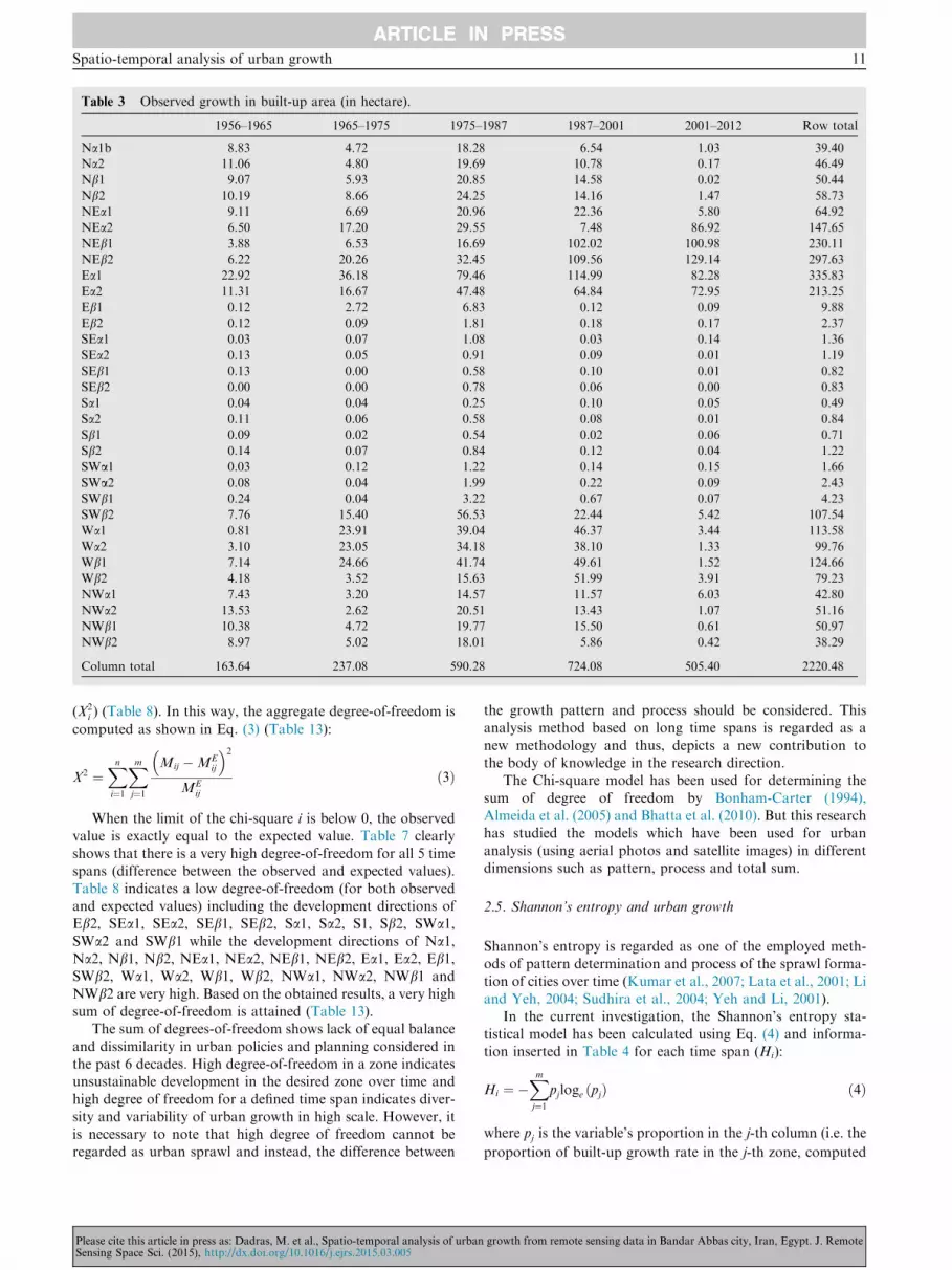
were calculated (Table 3). The percentage of increase in the

built-up regions is illustrated in Table 4, which also signifies

the rate of urban growth. From the table, it can be clearly seen

that the urban growth rate was decreasing gradually. In this

study, unusual urban growth rate was observed during the past

6 decades from 28.77% (2001–2012) which is the minimum to

122.67% (1975–1987) which is the maximum. Although the

available findings indicate a reduction of urban growth rate

over time, it does not necessarily show any regular compres-

sion and suitable urban sprawl. Therefore, the need for further

analysis is evident.

2.3. The difference between the observed and expected urban

growth

In an attempt to outline the different properties of growth, the

observed and the expected growth rates have to be ascertained

and observed. Table 3 illustrates the observed growth of the

usage of urban land. Here, the expected growth is computed

using Eq. (1); where Table 3 is regarded as matrix M with ele-

ments Mij, where i ¼ 1; 2; . . . ; n (the time span of the analysis,

Table rows) and j ¼ 1; 2; . . . ;m (specific zone, Table columns).

The expected growth of the built-up regions per variable is

computed by multiplying the special time span of the analysis

by the defined zone and dividing it by its total sum (Almeida

et al., 2005):

MEij ¼

MSj �MS

j

Mg

ð1Þ

where, MSi ¼ row total

MSj ¼ column total

Mg ¼ grand total ¼X

n

i¼1

X

m

j¼1

Mij

Figure 4 The Flowchart of image analysis.

8 M. Dadras et al.

ARTICLE IN PRESS



The result obtained from calculations using Eq. (1), which

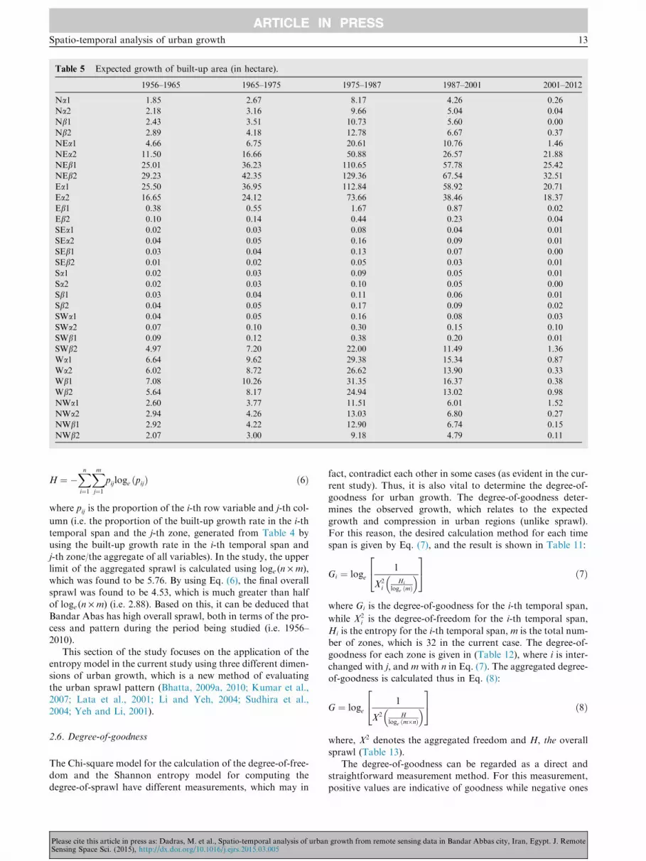
gives the expected growth is illustrated in Table 5. By subtract-

ing Table 3 (the observed built-up) from Table 4 (the expected

built-up), Table 6 is created. Table 6 illustrates the difference

between the urban growth per zone per time span. The nega-

tive results are indicative of a lower growth rate while the posi-

tive growth rate indicates urban growth. The degree of

deviation is another parameter that has been studied in the

current research. Here, it can be seen that the observed urban

growth deviated significantly from the expected growth in cer-

tain areas. This marked deviation is indicative of the freedom

of the variable. In the case of high deviation, it can be argued

that the desired variable is independent of other similar groups

of the variables. Nevertheless, only 5 time spans and one

degree of freedom are found in the analysis. Increase of time

spans in the analysis can help understand the behavior of the

independent variables. Specifically, 5 time spans have been

studied for analysis considering data availability in the defined

time intervals. It is necessary to note that the results of the

built-up expected zones have been based on the mentioned

analysis and statistical method irrespective of urban planning

and policies over time. It can be easily noted that the presence

of suitable regions for the development of each zone is differ-

ent from each other. Hence, urban planning and policymaking

toward the expected urban growth of the city should be

applied for promoting statistical analysis in the studied zones.

The zones which have the lowest value of suitable lands for

development clearly have the lowest expected growth. This

method also takes into consideration the land available for

development.

2.4. Pearson’s chi-square statistics and urban growth

The Pearson’s chi-square distribution employs the freedom

between variable pairs to describe the change in land use

within the same class (Almeida et al., 2005); using the

relation ðObserved� ExpectedÞ2=Expected. This relation

shows freedom or degree of deviation of the observed

urban growth compared with the expected urban growth.

The observed and the expected growth rates are displayed

in Table 3 and Table 7, respectively. Here, the Chi-square

statistical relation has been calculated for each time span

of (X2i ) based on Eq. (2) and its results are shown in

Table 7:

X2i ¼

X

m

j¼1

Mj �MEj

� �2

MEj

ð2Þ

Figure 5 Classified images of six temporal instants showing built-up areas and non-built-up area.


ARTICLE IN PRESS



where, X2i is the degree-of-freedom for the i-th temporal span,

while Mj is the observed built-up area in the j-th column for a

specific row, MEj is the expected built-up area in the j-th

column for a specific row. Hence, with a change in j (column)

by i (row), and m (number of columns) by n (number of rows)

in Eq. (2), the degree-of-freedom can be characterized per zone

Figure 6 Radar chart showing the built-up area in the different directions.

10 M. Dadras et al.

ARTICLE IN PRESS



(X2i ) (Table 8). In this way, the aggregate degree-of-freedom is

computed as shown in Eq. (3) (Table 13):

X2 ¼X

n

i¼1

X

m

j¼1

Mij �MEij

� �2

MEij

ð3Þ

When the limit of the chi-square i is below 0, the observed

value is exactly equal to the expected value. Table 7 clearly

shows that there is a very high degree-of-freedom for all 5 time

spans (difference between the observed and expected values).

Table 8 indicates a low degree-of-freedom (for both observed

and expected values) including the development directions of

Eb2, SEa1, SEa2, SEb1, SEb2, Sa1, Sa2, S1, Sb2, SWa1,

SWa2 and SWb1 while the development directions of Na1,

Na2, Nb1, Nb2, NEa1, NEa2, NEb1, NEb2, Ea1, Ea2, Eb1,

SWb2, Wa1, Wa2, Wb1, Wb2, NWa1, NWa2, NWb1 and

NWb2 are very high. Based on the obtained results, a very high

sum of degree-of-freedom is attained (Table 13).

The sum of degrees-of-freedom shows lack of equal balance

and dissimilarity in urban policies and planning considered in

the past 6 decades. High degree-of-freedom in a zone indicates

unsustainable development in the desired zone over time and

high degree of freedom for a defined time span indicates diver-

sity and variability of urban growth in high scale. However, it

is necessary to note that high degree of freedom cannot be

regarded as urban sprawl and instead, the difference between

the growth pattern and process should be considered. This

analysis method based on long time spans is regarded as a

new methodology and thus, depicts a new contribution to

the body of knowledge in the research direction.

The Chi-square model has been used for determining the

sum of degree of freedom by Bonham-Carter (1994),

Almeida et al. (2005) and Bhatta et al. (2010). But this research

has studied the models which have been used for urban

analysis (using aerial photos and satellite images) in different

dimensions such as pattern, process and total sum.

2.5. Shannon’s entropy and urban growth

Shannon’s entropy is regarded as one of the employed meth-

ods of pattern determination and process of the sprawl forma-

tion of cities over time (Kumar et al., 2007; Lata et al., 2001; Li

and Yeh, 2004; Sudhira et al., 2004; Yeh and Li, 2001).

In the current investigation, the Shannon’s entropy sta-

tistical model has been calculated using Eq. (4) and informa-

tion inserted in Table 4 for each time span (Hi):

Hi ¼ �X

m

j¼1

pjloge ðpjÞ ð4Þ

where pj is the variable’s proportion in the j-th column (i.e. the

proportion of built-up growth rate in the j-th zone, computed

Table 3 Observed growth in built-up area (in hectare).

1956–1965 1965–1975 1975–1987 1987–2001 2001–2012 Row total

Na1b 8.83 4.72 18.28 6.54 1.03 39.40

Na2 11.06 4.80 19.69 10.78 0.17 46.49

Nb1 9.07 5.93 20.85 14.58 0.02 50.44

Nb2 10.19 8.66 24.25 14.16 1.47 58.73

NEa1 9.11 6.69 20.96 22.36 5.80 64.92

NEa2 6.50 17.20 29.55 7.48 86.92 147.65

NEb1 3.88 6.53 16.69 102.02 100.98 230.11

NEb2 6.22 20.26 32.45 109.56 129.14 297.63

Ea1 22.92 36.18 79.46 114.99 82.28 335.83

Ea2 11.31 16.67 47.48 64.84 72.95 213.25

Eb1 0.12 2.72 6.83 0.12 0.09 9.88

Eb2 0.12 0.09 1.81 0.18 0.17 2.37

SEa1 0.03 0.07 1.08 0.03 0.14 1.36

SEa2 0.13 0.05 0.91 0.09 0.01 1.19

SEb1 0.13 0.00 0.58 0.10 0.01 0.82

SEb2 0.00 0.00 0.78 0.06 0.00 0.83

Sa1 0.04 0.04 0.25 0.10 0.05 0.49

Sa2 0.11 0.06 0.58 0.08 0.01 0.84

Sb1 0.09 0.02 0.54 0.02 0.06 0.71

Sb2 0.14 0.07 0.84 0.12 0.04 1.22

SWa1 0.03 0.12 1.22 0.14 0.15 1.66

SWa2 0.08 0.04 1.99 0.22 0.09 2.43

SWb1 0.24 0.04 3.22 0.67 0.07 4.23

SWb2 7.76 15.40 56.53 22.44 5.42 107.54

Wa1 0.81 23.91 39.04 46.37 3.44 113.58

Wa2 3.10 23.05 34.18 38.10 1.33 99.76

Wb1 7.14 24.66 41.74 49.61 1.52 124.66

Wb2 4.18 3.52 15.63 51.99 3.91 79.23

NWa1 7.43 3.20 14.57 11.57 6.03 42.80

NWa2 13.53 2.62 20.51 13.43 1.07 51.16

NWb1 10.38 4.72 19.77 15.50 0.61 50.97

NWb2 8.97 5.02 18.01 5.86 0.42 38.29

Column total 163.64 237.08 590.28 724.08 505.40 2220.48


ARTICLE IN PRESS



from Table 4 using the built-up growth rate in j-th zone/the

aggregated built-up growth rates across the zones). Here, m

denotes the summation of zones, which is 32 in the current

study. The degree-of-sprawl in this case, is derived from the

entropy value, which falls within the limit 0 6 x 6 loge ðmÞ.At 0, the built-up distribution is said to be compact, while

sparse distribution increases with increasing divergence from

zero.

Table 9 illustrates that the attained entropy from the study

is greater than half of the index logeðmÞ. As such, one can con-

clude that the Bandar Abbas city underwent a sprawl during

the past 6 decades. However, urban sprawl has been reduced

over time. Based on the research findings by Richardson

et al. (2000), towns and cities in developing countries are being

compressed considering the structure of their formation based

on decentralization and there is evidence that the general trend

of the developing countries is being more compressed. Based

on the studies conducted by Iranian Ministry of Road and

Urban Development, it is shown that most cities of the coun-

tries are experiencing increasing sprawl trend. According to the

performance analysis, it can be argued that the Bandar Abbas

city has limited chances of sprawl considering the trend during

the past periods due to limitations in development in the vari-

ous geographical directions; depicting a descending trend over

time. These findings also show that administrative boundaries

cannot give the real understanding of urban growth. The result

further indicates that the Bandar Abbas city has high sprawl.

However, where the entropy value is below half of logeðmÞ,it can be argued that the city has no chance of sprawl. Eq.

(5), which is the revised form of Eq. (4) is used for determining

the entropy of each zone:

Hj ¼ �X

n

i¼1

piloge ðpiÞ ð5Þ

where pi is the proportion of the variable in the i-th row (i.e.

proportion of built-up growth rate in i-th temporal span, com-

puted from Table 4 using the built-up growth rate in the i-th

temporal span/the aggregated built-up growth rate across the

time spans). Here, n is the total number of temporal spans,

which is 5 in the current study.

Table 10 illustrates that more than half of loge ðmÞ entropyvalues are achieved, implying that the zones are being

sprawled. Based on the performed analysis, it can be argued

that the Bandar Abbas city had a general sprawl in all the geo-

graphical directions, particularly in the eastern and northern

zones of the city. For this reason, it had lower sprawl in the

western direction, and particularly the southern direction

based on the limitations of the seashore and the military zone

of the marine force. The total aggregated sprawl can be deter-

mined using the relation:

Table 4 Built-up growth rate of fifty-six-yearly periods (in percent).

1956–1965 1965–1975 1975–1987 1987–2001 2001–2012

Na1 186.50 34.80 35.79 6.18 3.90

Na2 288.16 32.24 54.72 �0.03 0.54

Nb1 154.74 39.71 69.92 0.52 0.05

Nb2 189.22 55.60 58.40 2.50 3.72

NEa1 176.64 46.87 106.68 30.48 10.26

NEa2 111.01 139.34 25.31 62.23 144.69

NEb1 61.83 64.27 611.12 78.78 47.58

NEb2 104.21 166.26 337.63 65.93 54.80

Ea1 112.64 83.60 144.71 29.12 32.77

Ea2 57.98 54.10 136.56 34.33 48.35

Eb1 2.94 65.96 1.69 22.80 1.11

Eb2 7.71 5.16 9.76 �16.99 10.52

SEa1 3.08 6.95 2.65 �16.99 15.71

SEa2 18.35 5.53 9.57 �22.50 1.64

SEb1 27.53 0.00 17.25 20.06 1.08

SEb2 0.00 0.00 7.36 �14.78 0.00

Sa1 24.52 20.24 40.51 �28.70 19.86

Sa2 27.58 12.37 14.26 �13.88 1.22

Sb1 20.41 3.39 2.82 23.30 8.57

Sb2 21.80 9.48 14.41 �23.27 5.87

SWa1 2.67 11.38 11.31 �0.45 11.24

SWa2 4.47 2.25 11.12 �14.40 4.70

SWb1 7.99 1.21 20.85 �19.92 2.13

SWb2 23.24 37.42 39.70 12.68 6.09

Wa1 5.69 158.10 118.78 8.14 3.73

Wa2 38.66 206.96 111.46 11.44 1.65

Wb1 71.77 144.38 118.85 4.41 1.59

Wb2 52.78 29.06 332.53 8.27 5.34

NWa1 188.83 28.20 79.44 14.13 20.20

NWa2 310.13 14.64 65.47 16.16 2.73

NWb1 222.41 31.41 78.42 12.99 1.53

NWb2 222.72 38.64 32.54 21.70 1.45

The city 86.32 67.12 122.67 28.49 29.92

12 M. Dadras et al.

ARTICLE IN PRESS



H ¼ �X

n

i¼1

X

m

j¼1

pijloge ðpijÞ ð6Þ

where pij is the proportion of the i-th row variable and j-th col-

umn (i.e. the proportion of the built-up growth rate in the i-th

temporal span and the j-th zone, generated from Table 4 by

using the built-up growth rate in the i-th temporal span and

j-th zone/the aggregate of all variables). In the study, the upper

limit of the aggregated sprawl is calculated using loge (n · m),

which was found to be 5.76. By using Eq. (6), the final overall

sprawl was found to be 4.53, which is much greater than half

of loge (n · m) (i.e. 2.88). Based on this, it can be deduced that

Bandar Abas has high overall sprawl, both in terms of the pro-

cess and pattern during the period being studied (i.e. 1956–

2010).

This section of the study focuses on the application of the

entropy model in the current study using three different dimen-

sions of urban growth, which is a new method of evaluating

the urban sprawl pattern (Bhatta, 2009a, 2010; Kumar et al.,

2007; Lata et al., 2001; Li and Yeh, 2004; Sudhira et al.,

2004; Yeh and Li, 2001).

2.6. Degree-of-goodness

The Chi-square model for the calculation of the degree-of-free-

dom and the Shannon entropy model for computing the

degree-of-sprawl have different measurements, which may in

fact, contradict each other in some cases (as evident in the cur-

rent study). Thus, it is also vital to determine the degree-of-

goodness for urban growth. The degree-of-goodness deter-

mines the observed growth, which relates to the expected

growth and compression in urban regions (unlike sprawl).

For this reason, the desired calculation method for each time

span is given by Eq. (7), and the result is shown in Table 11:

Gi ¼ loge1

X2i

Hi

loge ðmÞ

� �

2

4

3

5 ð7Þ

where Gi is the degree-of-goodness for the i-th temporal span,

while X2i is the degree-of-freedom for the i-th temporal span,

Hi is the entropy for the i-th temporal span, m is the total num-

ber of zones, which is 32 in the current case. The degree-of-

goodness for each zone is given in (Table 12), where i is inter-

changed with j, and m with n in Eq. (7). The aggregated degree-

of-goodness is calculated thus in Eq. (8):

G ¼ loge1

X2 Hloge ðm�nÞ

� �

2

4

3

5 ð8Þ

where, X2 denotes the aggregated freedom and H, the overall

sprawl (Table 13).

The degree-of-goodness can be regarded as a direct and

straightforward measurement method. For this measurement,

positive values are indicative of goodness while negative ones

Table 5 Expected growth of built-up area (in hectare).

1956–1965 1965–1975 1975–1987 1987–2001 2001–2012

Na1 1.85 2.67 8.17 4.26 0.26

Na2 2.18 3.16 9.66 5.04 0.04

Nb1 2.43 3.51 10.73 5.60 0.00

Nb2 2.89 4.18 12.78 6.67 0.37

NEa1 4.66 6.75 20.61 10.76 1.46

NEa2 11.50 16.66 50.88 26.57 21.88

NEb1 25.01 36.23 110.65 57.78 25.42

NEb2 29.23 42.35 129.36 67.54 32.51

Ea1 25.50 36.95 112.84 58.92 20.71

Ea2 16.65 24.12 73.66 38.46 18.37

Eb1 0.38 0.55 1.67 0.87 0.02

Eb2 0.10 0.14 0.44 0.23 0.04

SEa1 0.02 0.03 0.08 0.04 0.01

SEa2 0.04 0.05 0.16 0.09 0.01

SEb1 0.03 0.04 0.13 0.07 0.00

SEb2 0.01 0.02 0.05 0.03 0.01

Sa1 0.02 0.03 0.09 0.05 0.01

Sa2 0.02 0.03 0.10 0.05 0.00

Sb1 0.03 0.04 0.11 0.06 0.01

Sb2 0.04 0.05 0.17 0.09 0.02

SWa1 0.04 0.05 0.16 0.08 0.03

SWa2 0.07 0.10 0.30 0.15 0.10

SWb1 0.09 0.12 0.38 0.20 0.01

SWb2 4.97 7.20 22.00 11.49 1.36

Wa1 6.64 9.62 29.38 15.34 0.87

Wa2 6.02 8.72 26.62 13.90 0.33

Wb1 7.08 10.26 31.35 16.37 0.38

Wb2 5.64 8.17 24.94 13.02 0.98

NWa1 2.60 3.77 11.51 6.01 1.52

NWa2 2.94 4.26 13.03 6.80 0.27

NWb1 2.92 4.22 12.90 6.74 0.15

NWb2 2.07 3.00 9.18 4.79 0.11


ARTICLE IN PRESS



are indicative of badness. This goodness or badness can be

determined from the information in Tables 11–13. Here, the

variables of degree-of-goodness can be positive or negative

good depending on the zone and time span. From the result,

it can be argued that urban boundaries had no good experience

of urban growth trend in the time span of 1956–2012. Separate

analysis of each zone out of the desired zones also shows simi-

lar results. Although southeastern, southern and southwestern

zones have positive values, high positive values are found only

in zones Sa1 and SEb2. As Table 13 shows, the overall good-

ness depicts a worse condition.

3. Discussion

It could be recalled that the current study has been conducted

in 5 time spans using aerial photos and satellite images for a

56-year time interval. Certainly, better results will be obtained

if more images were studied and analyzed in shorter time

spans. Also, the reliability of the statistical analysis will

improve by increasing the number of variables. Based on the

mentioned research method, the studied zone was divided into

32 equal parts in different geographical directions to determine

urban sprawl trend. In addition, the studied zone was further

divided into concentric circles, for better results and under-

standing of urban growth trend in Bandar Abbas from the past

to the present. In different zones, there are different levels of

compression and this factor causes varying urban growth pat-

terns. As such, a unique policy designed for a city cannot be

suitably applied for other cities with equal effectiveness.

As mentioned earlier, the main goal of this study is to inves-

tigate new analysis methods based on 5 time spans and 32 geo-

graphical directions in urban growth trend instead of urban

comprehensive studies. It is necessary to note that if a city is

divided into circular zones and sections based on geographical

directions, distance to commercial zones will be directly con-

sidered in a definite zone and this may be very useful in trend

analysis. It is very important to specify the distance to centers

of commercial zones for determining changes of urban density.

It is also necessary to note that the center of the circle and the

desired zones have been considered based on the primary goal

of the city formation. In this study, it is assumed that there is

an equal possibility of growth in all directions of the city center

Table 6 Difference between observed and expected built-up growth (in hectare).

1956–1965 1965–1975 1975–1987 1987–2001 2001–2012

Na1 6.98 2.05 �1.62 �2.73 0.77

Na2 8.87 1.64 1.12 �5.03 0.11

Nb1 6.64 2.41 3.85 �5.42 0.01

Nb2 7.31 4.48 1.38 �5.71 1.10

NEa1 4.46 �0.06 1.75 2.44 4.34

NEa2 �5.00 0.54 �43.40 �3.52 65.04

NEb1 �21.12 �29.70 �8.64 35.75 75.56

NEb2 �23.01 �22.09 �19.80 26.09 96.63

Ea1 �2.58 �0.76 2.15 �2.29 61.57

Ea2 �5.34 �7.45 �8.82 0.09 54.59

Eb1 �0.26 2.17 �1.55 0.71 0.07

Eb2 0.02 �0.06 �0.26 0.43 0.13

SEa1 0.01 0.04 �0.05 0.02 0.03

SEa2 0.10 �0.01 �0.08 0.04 0.04

SEb1 0.10 �0.04 �0.03 0.07 0.01

SEb2 �0.01 �0.02 0.01 0.02 0.03

Sa1 0.02 0.01 0.01 �0.01 0.02

Sa2 0.09 0.03 �0.02 �0.04 0.01

Sb1 0.06 �0.02 �0.10 0.07 0.04

Sb2 0.10 0.02 �0.05 �0.05 0.07

SWa1 �0.01 0.07 �0.02 �0.07 0.10

SWa2 0.02 �0.05 �0.07 �0.06 0.28

SWb1 0.15 �0.08 0.29 �0.13 0.03

SWb2 2.79 8.19 0.44 �1.47 4.05

Wa1 �5.82 14.30 16.99 �8.39 2.57

Wa2 �2.91 14.33 11.48 �5.63 0.99

Wb1 0.05 14.40 18.26 �12.34 1.14

Wb2 �1.45 �4.65 27.04 �7.43 2.92

NWa1 4.83 �0.56 0.06 �2.32 4.51

NWa2 10.58 �1.65 0.40 �1.32 0.80

NWb1 7.46 0.50 2.60 �2.16 0.46

NWb2 6.89 2.02 �3.31 0.39 0.31

Table 7 Degree-of-freedom for urban growth in each

temporal span.

Time span Freedom ðX2i Þ

1956–1965 242.83

1965–1975 135.17

1975–1987 102.45

1987–2001 74.49

2001–2012 1124.54

14 M. Dadras et al.

ARTICLE IN PRESS



and that no commercial center, special lands, road network

and other variables have unequal growth. However, it is not

necessary to consider urban boundary based on a circular

zone. Instead, natural boundaries or urban boundaries can

be used and divided it into different sections. Administrative

boundaries can also be considered (although they do not

reflect dynamicity of urban sprawl), which in fact, reflects eco-

nomic and social dependencies and independencies. Natural

boundaries are seldom affected by data of social and economic

variables. In many countries such as Iran, data relating to

socioeconomic variables which relate to administrative bound-

aries are accessible. For this reason, the city was divided into

24 parts for analyzing urban growth pattern using social-eco-

nomic variables and Shannon’s entropy model considering

the administrative boundary of Bandar Abbas. The models

shown in the present study are not directly dependent on the

selection of the studied zone and its divisions. They are also

not dependent on the number of divisions. Of course, it is

necessary to note that the more the number of divisions, the

more accurate the result. The performed measurements of

the study are based on the per zone built-up regions.

Anyway, the regions which have accessible lands for develop-

ment are not equal in each zone. Therefore, it is better to cal-

culate three measurement methods of freedom, sprawl, and

goodness based on percentage of the built-up areas in each

zone. This percentage can be calculated using Eq. (9):

ðBuilt-up area within a zoneÞ

ðtotal area of the zone�non-development land within the zoneÞ

�100

ð9Þ

Table 8 Degree-of-freedom for urban growth in each zone.

Zone Freedom ðX2i Þ

Na1 32.34

Na2 42.39

Nb1 26.49

Nb2 31.59

NEa1 17.86

NEa2 233.01

NEb1 289.58

NEb2 329.96

Ea1 183.40

Ea2 167.32

Eb1 11.04

Eb2 1.38

SEa1 0.21

SEa2 0.44

SEb1 0.44

SEb2 0.13

Sa1 0.10

Sa2 0.44

Sb1 0.47

Sb2 0.52

SWa1 0.46

SWa2 0.92

SWb1 0.72

SWb2 23.12

Wa1 48.43

Wa2 35.15

Wb1 43.50

Wb2 45.26

NWa1 23.35

NWa2 41.35

NWb1 21.71

NWb2 26.44

Table 9 Shannon’s entropy of each temporal span.

Time span Entropy (Hi) loge ðmÞ loge ðmÞ=2

1956–1965 2.923 3.58 1.79

1965–1975 2.912 3.58 1.79

1975–1987 2.761 3.58 1.79

1987–2001 2.966 3.58 1.79

2001–2012 2.491 3.58 1.79

Table 10 Shannon’s entropy for different zones.

Zone Entropy (Hi) loge ðmÞ loge ðmÞ=2

Na1 0.93 1.61 0.80

Na2 0.70 1.61 0.80

Nb1 0.96 1.61 0.80

Nb2 1.02 1.61 0.80

NEa1 1.28 1.61 0.80

NEa2 1.48 1.61 0.80

NEb1 1.00 1.61 0.80

NEb2 1.38 1.61 0.80

Ea1 1.44 1.61 0.80

Ea2 1.48 1.61 0.80

Eb1 0.83 1.61 0.80

Eb2 1.33 1.61 0.80

SEa1 1.54 1.61 0.80

SEa2 1.50 1.61 0.80

SEb1 1.14 1.61 0.80

SEb2 1.08 1.61 0.80

Sa1 1.46 1.61 0.80

Sa2 1.19 1.61 0.80

Sb1 1.33 1.61 0.80

Sb2 1.48 1.61 0.80

SWa1 1.38 1.61 0.80

SWa2 1.38 1.61 0.80

SWb1 1.01 1.61 0.80

SWb2 1.44 1.61 0.80

Wa1 0.93 1.61 0.80

Wa2 1.05 1.61 0.80

Wb1 1.14 1.61 0.80

Wb2 0.77 1.61 0.80

NWa1 1.18 1.61 0.80

NWa2 0.78 1.61 0.80

NWb1 0.99 1.61 0.80

NWb2 0.95 1.61 0.80

Table 11 Degree-of-goodness for urban growth in each

temporal span.

Time span Goodness (Gi)

1956–1965 �6.015

1965–1975 �5.426

1975–1987 �5.095

1987–2001 �4.848

2001–2012 �7.388


ARTICLE IN PRESS



It is necessary to note that the area of the developed lands

cannot be directly measured with aerial photos and satellite

images. Different factors may play a role in non-sprawl of a

region, which include natural factors (rivers, coasts and rough

lands), ownership (land ownership by military forces), policies

of government (for protecting open spaces, aquatic, agricul-

tural and green spaces), legal disputes on lands, etc.

Therefore, it may be hard to collect this dataset in different

time spans. However, if these data are accessible, the percent-

age of the non-built areas in the desired zones will attain more

accuracy.

The method used in the current study may be criticized as a

result of its simplicity in the analysis of urban growth. The rea-

sons which can be effective are failure to use road network, dis-

tribution of commercial centers in urban boundary, special

lands, change of land uses over time and many other cases

which are mentioned in the introduction of the paper and have

been studied and analyzed by researchers. It should be noted

that many of the cities in the developing countries have been

sprawled without sprawl plan over time. In most scenarios,

these cities do not have any historical data of urban sprawl

or related land use data over a period of time. As such, the

majority of the spatio-statistical models are not suitable for

studying urban growth patterns. In addition, many of the

urban managers (for example: Bandar Abbas) do not have

enough ability and proficiency to use the models, tools and

new technologies such as geographic information system and

remote sensing. Therefore, it is necessary to note that urban

growth pattern should be determined based on simple analysis

methods and the minimum input data should be employed.

For this reason, one can study and analyze urban growth trend

in the past and at present using the required minimum input

data and aerial photos and satellite images based on the meth-

ods used and proposed in this study.

In this study, the proposed method determines the degree of

goodness, however, one of the main limitations of the method

is inability to apply and calculate the past political variables.

Although there may be planned policies for the development

of cities in industrial countries, the developing cities lack such

policies in most cases and growth trend is completely free.

Therefore, methods and approaches used in this study could

be useful and applicable to numerous cities across the develop-

ing countries. This, however, does not imply that the models

presented cannot be used for determining degree of goodness

in cities of the industrialized countries. Because there are no

predetermined growth policy and planning for Bandar

Abbas, the expected urban growth has been calculated using

statistical methods and based on urban growth trend in the

past and present (Eq. (1)). In many cities of the industrial

countries, the expected urban growth has been predetermined

and planned for the future. Therefore, the predetermined val-

ues should be considered considering the variables available in

Eq. (1) for such cities. As a result, the quantity of degree-

of-freedom and degree-of-goodness will be influenced by these

variables. Even though the primary goal of this study is to

investigate new methods and models, the results obtained have

analyzed urban growth pattern in Bandar Abbas. The infor-

mation obtained from the research models can be used in the

future by local planners and managers in understanding

sprawling trend of the urban boundary in the past and present

for preparing development projects. In fact, understanding

urban growth complexity allows one to be familiar with some

necessary tools which have been introduced in recent years

with efficient, stable and realistic principles.

Finally, the degree-of-goodness shows sustainable develop-

ment can be discussed and judged in terms of sustainability

measurement methods based on experimental evidence. Since

the degree-of-goodness is based on two observed and expected

variables calculated, this method is introduced as a direct mea-

surement of urban growth. Certainly, most analyses can show

correlation between degree-of-goodness and sustainable urban

growth. However, in-depth analysis of sustainable develop-

ment is not within the scope of the current study. In fact, sus-

tainable development is known as a multilateral process and

considers development of all aspects which are effective in

the life of humans and creatures (Hasna, 2007). This means

that it settles conflicts between different competitive goals

which include concurrent priorities of environmental quality,

economic welfare and social justice. For this reason, the trend

is a continual process. Urban growth is very important for

achieving sustainable development, and requires the obser-

vance of all planned principles and performance of the

predetermined policies (by governments in future). However,

Table 12 Degree-of-goodness for urban growth in each zone.

Zone Goodness (Gi)

Na1 �2.93

Na2 �2.92

Nb1 �2.76

Nb2 �2.99

NEa1 �2.65

NEa2 �5.36

NEb1 �5.20

NEb2 �5.65

Ea1 �5.10

Ea2 �5.04

Eb1 �1.73

Eb2 �0.13

SEa1 1.62

SEa2 0.90

SEb1 1.17

SEb2 2.42

Sa1 2.45

Sa2 1.12

Sb1 0.96

Sb2 0.74

SWa1 0.94

SWa2 0.24

SWb1 0.80

SWb2 �3.03

Wa1 �3.33

Wa2 �3.14

Wb1 �3.43

Wb2 �3.07

NWa1 �2.84

NWa2 �3.00

NWb1 �2.59

NWb2 �2.74

Table 13 Overall degree-of-freedom, entropy, and degree-of-

goodness.

Degree-of-freedom (X2) Entropy (H) Degree-of-goodness (G)

1679.483 4.530 �7.313

16 M. Dadras et al.

ARTICLE IN PRESS



the trend of achieving sustainable development is not naturally

a fixed process. Instead, it is a multidimensional set which is

based on the interaction between the characteristics and speci-

fications of systems in future. It can, therefore, be argued that

the degree-of-goodness models do not have the capacity to

determine the sustainable development directly. Instead, it is

likely that the degree-of-goodness model can be converted into

one of the determined indices of sustainable development.

However, it will be better to create correlation between the

two for determining the reliability before such conclusion.

4. Conclusions

The goal of the current study is to investigate the urban growth

of the Iranian city of Bandar Abbas using the retrieved data

spanning 6 decades using aerial photos and satellite images

and new statistical methods. In the study, various statistical

models were employed for studying and analyzing urban

growth based on aspects of the pattern including general pro-

cesses and conditions. The models showed that the city exhibits

high degree of freedom and sprawl. Moreover, the urban

sprawl trend was found to reduce over time while the degree

of freedom trend was found to increase. Specifically, the

degree-of-goodness was found to be improper, with a warning

condition. Also, the goodness of the urban growth showed a

descending trend despite the reduction of urban growth rate.

The result further showed that the proposed models can be

useful tools for identifying urban growth patterns and their

general tendencies. The models, which have been used for ana-

lyzing urban growth based on specified measurement scales

and variables of the observed built zones and expected built

zones, include the Person’s chi-square, Shannon’s entropy

and degree-of-goodness. The models shown in the study have

been devised experimentally and not presented by the strong

theories which are limited to a special zone. Therefore, they

can be easily applied in other cities which have spatial and

attribute data from the past and present, particularly the devel-

oping countries. As such, the new hypothesis, which can be put

forward based on the analysis in the study, is that the degree-

of-goodness model can be regarded as a sustainable develop-

ment index and constitutes a vital tool to future researchers.

The current study also focused on a special scope of the

research, which is the application of the shown models for

determining and identifying urban growth trend of the

Bandar Abbas city, which can be used by urban planners

and managers. The scope of the study is limited to the applica-

tion of the referred models for urban planners and other users

in developing countries; thanks to the motivation from the

urban growth analysis theories and models developed by other

researchers.

References

Al-Awadhi, T., 2007. Monitoring and modeling urban expansion

using GIS and RS: Case study from Muscat, Oman. In:

Proceedings of Urban Remote Sensing Joint Event. 11–13 April,

2007, Paris, France.

Alberti, M., 2005. The effects of urban patterns on ecosystem

function. Int. Reg. Sci. Rev. 28 (2), 168–192.

Almeida, C.M., Monteiro, A.M.V., Mara, G., Soares-Filho, B.S.,

Cerqueira, G.C., Pennachin, C.S.L., 2005. GIS and remote sensing

as tools for the simulation of urban land-use change. Int. J. Remote

Sens. 26 (4), 759–774.

Angel, S., Sheppard, S.C., Civco, D.L., 2005. The dynamics of Global

Urban Expansion. Available from. Washington D.C.: Transport

and Urban Development Department, The World Bank. <http://

www.citiesalliance.org/doc/resources/upgrading/urban-expan-

sion/worldbank reportsept2005.pdf p. 200/>.

Belal, A.A., Moghanm, F.S., 2011. Detecting urban growth using

remote sensing and GIS techniques in Al Gharbiya governorate.

Egypt. J. Remote Sens. Space Sci. 14, 73–79.

Barnes, K.B., Morgan, J.M., III, Roberge, M.C., Lowe, S., 2001.

Sprawl Development: Its Patterns, Consequences, and

Measurement. A White Paper. Available from: Towson

University <http://chesapeake.towson.edu/landscape/ur-

bansprawl/download/Sprawl_white_paper.pdf/> (accessed

10.01.07).

Batisani, N., Yarnal, B., 2009. Urban expansion in centre county,

Pennsylvania: spatial dynamics and landscape transformations.

Appl. Geogr. 29 (2), 235–249.

Batty, M., Howes, D., 2001. Predicting temporal patterns in urban

development from remote imagery. In: Donnay, J.P., Barnsley,

M.J., Longley, P.A. (Eds.), Remote Sensing and Urban Analysis.

Taylor & Francis, London, pp. 185–204.

Batty, M., Xie, Y., 1997. Possible urban automata. Environ. Plann. B

24, 175–192.

Belkina, T.D., 2007. Diagnosing urban development by an indicator

system. Stud. Russ. Econ. Dev. 18 (2), 162–170.

Benati, S., 1997. A cellular automaton for the simulation of competi-

tive location. Environ. Plann. B. 24, 205–218.

Bhatta, B., 2009a. Analysis of urban growth pattern using remote

sensing and GIS: a case study of Kolkata, India. Int. J. Remote

Sens. http://dx.doi.org/10.1080/01431160802651967.

Bhatta, B., 2009c. Modelling of urban growth boundary using

geoinformatics. Int. J. Digit. Earth. http://dx.doi.org/10.1080/

17538940902971383.

Bhatta, B., 2010. Analysis of Urban Growth and Sprawl from Remote

Sensing Data. Springer-Verlag, Berlin, Heidelberg.

Bhatta, B., Saraswati, S., Bandyopadhyay, D., 2010. Quantifying the

degree-of-freedom, degree-of-sprawl, and degree-of-goodness of

urban growth from remote sensing data. Appl. Geogr. 30 (1), 96–

111.

Bonham-Carter, G.F., 1994. Geographic Information Systems for

Geoscientists: Modelling with GIS. Pergamon, Ontario, p. 398.

Chen, C., 2003. Frontiers of Remote Sensing Information Processing.

World Scientific, p. 614.

Cho, S., Lambert, D.M., Roberts, R.K., Kim, S.G., 2010. Moderating

urban sprawl: is there a balance between shared open space and

housing parcel size? J. Econ. Geogr. 10 (5), 763–783.

Clark, D., 1982. Urban Geography: An Introductory Guide. Taylor &

Francis, p. 231.

Clark, W.A., Hosking, P.L., 1986. Statistical Methods for

Geographers. John Wiley and Sons, New York, 518 pp.

Clarke, K.C., Hoppen, S., Gaydos, L., 1997. A self-modifying cellular

automaton model of historical urbanization in the San Francisco

Bay area. Environ. Plann. B. 24, 247–261.

Deadman, P.D., Brown, R.D., Gimblett, H.R., 1993. Modelling rural

residential settlement patterns with cellular automata. J. Environ.

Manage. 37, 147–160.

Deep, S., Saklani, A., 2014. Urban sprawl modeling using cellular

automata. Egypt. J. Remote Sens. Space Sci. 17, 179–187.

Deng, J., Wang, K., Hong, Y., Jia, G., 2009. Spatio-temporal

dynamics and evolution of land use change and landscape pattern

in response to rapid urbanization. Landscape Urban Plann. 92,

187–198.

Dewan, A.M., Yamaguchi, Y., 2009. Land use and land cover change

in Greater Dhaka, Bangladesh: using remote sensing to promote

sustainable urbanization. Appl. Geogr. 29, 390–401.


ARTICLE IN PRESS


http://refhub.elsevier.com/S1110-9823(15)00008-3/h0010






http://www.citiesalliance.org/doc/resources/upgrading/urban-expansion/worldbank%20reportsept2005.pdf%20p.%20200/






http://chesapeake.towson.edu/landscape/urbansprawl/download/Sprawl_white_paper.pdf/

http://chesapeake.towson.edu/landscape/urbansprawl/download/Sprawl_white_paper.pdf/














http://dx.doi.org/10.1080/01431160802651967

http://dx.doi.org/10.1080/17538940902971383

http://dx.doi.org/10.1080/17538940902971383


































Donnay, J.P., Barnsley, M.J., Longley, P.A., 2001. Remote sensing

and urban analysis. In: Donnay, J.P., Barnsley, M.J., Longley, P.A.

(Eds.), Remote Sensing and Urban Analysis. Taylor and Francis,

London and New York, pp. 3–18.

Farhoudi, R., Zanganeh, S.S., Saed Moucheshi, R., 2009. Spatial

distribution of population in Iranian urban system. Q. Geogr. Res.

68, 55–68.

Fotheringham, A.S., Wegener, M., 2000. Spatial Models and GIS:

New Potential and New Models. Taylor and Francis, London, p.

279.

Galster, G., Hanson, R., Wolman, H., Coleman, S., Freihage, J., 2001.

Wrestling sprawl to the ground: defining and measuring an elusive

concept. House Policy Debate 12 (4), 681–717.

Griffith, D.A., 1988. Advanced Spatial Statistics: Special Topics in the

Exploration of Quantitative Spatial Data Series. Kluwer,

Dordrecht.

Hasna, A.M., 2007. Dimensions of sustainability. J. Eng. Sustainable

Dev. Energy Environ. Health 2 (1), 47–57.

Hedblom, M., Soderstrom, B., 2008. Woodlands across Swedish urban

gradients: status, structure and management implications.

Landscape Urban Plann. 84, 62–73.

Herold, M., Clarke, K.C., Scepan, J., 2002. Remote sensing and

landscape metrics to describe structures and changes in urban land

use. Environ. Plann. A. 34 (8), 1443–1458.

Herold, M., Goldstein, N.C., Clarke, K.C., 2003. The spatiotemporal

form of urban growth: measurement, analysis and modeling.

Remote Sens. Environ. 86, 286–302.

Herold,M.,Hemphill, J., Dietzel, C., Clarke, K.C., 2005. Remote sensing

derived mapping to support urban growth theory. Tempe, AZ, USA,

March 14–16, 2005. Available from: Proceedings of the ISPRS joint

conference 3rd International Symposium Remote Sensing and Data

FusionOverUrbanAreas, and 5th International SymposiumRemote

Sensing of Urban Areas (URS 2005). <www.isprs.org/commis-

sion8/workshop_urban/herold_hemphill_etal.pdf/>.

Iranian Statistic Center (2012). Census data. Tehran, Iran.

Iqbal, M.F., Khan, I.A., 2014. Spatiotemporal land use land cover

change analysis and erosion risk mapping of Azad Jammu and

Kashmir, Pakistan. Egypt. J. Remote Sens. Space Sci. 17, 209–229.

Ismail, M.H., Jusoff, K., 2008. Satellite data classification accuracy

assessment based from reference dataset. Int. J. Comput. Inf. Sci.

Eng. 2 (2), 96–102, <http://www.waset.org/ijcise/v2/v2-2-16.pdf/>.

Kumar, J.A.V., Pathan, S.K., Bhanderi, R.J., 2007. Spatio-temporal

analysis for monitoring urban growth – a case study of Indore city.

J. Indian Soc. Remote Sens. 35 (1), 11–20.

Landis, J., Zhang, M., 2000. Using GIS to improve urban activity and

forecasting models: three examples. In: Fotheringham, A.S.,

Wegener, M. (Eds.), Spatial Models and GIS: New Potential and

New Models. Taylor and Francis, London, pp. 63–81.

Lassila, K.D., 1999. The new suburbanites: how American plants and

animals are threatened by the sprawl. Amic J. 21, 16–22.

Lata, K.M., Rao, C.H.S., Prasad, V.K., Badarianth, K.V.S.,

Rahgavasamy, V., 2001. Measuring urban sprawl: a case study of

Hyderabad. GIS Dev. 5 (12), 26–29.

Litman, T., 2007. Evaluating Criticism of Smart Growth. Victoria

Transport Policy Institute.

Li, X., Yeh, A.G.O., 2002. Neural-network-based cellular automata

for simulating multiple land use changes using GIS. Int. J. Geogr.

Sci. 16, 323–343.

Li, X., Yeh, A.G.O., 2004. Analyzing spatial restructuring of land use

patterns in a fast growing region remote sensing and GIS.

Landscape Urban Plann. 69, 335–354.

Liu, J.G., 2000. Smoothing filter-based intensity modulation: a spectral

preserve image fusion technique for improving spatial details. Int.

J. Remote Sens. 21 (18), 3461–3472.

Lopez Sandoval, M.F., 2004. Agricultural and Settlement Frontiers in

the Tropical Andes: The Paramo Belt of Northern Ecuador, 1960–

1990. Regensburger Geographische Schriften. Heft 37. Institut fur

Geographie an der Universitat Regensburg, Germany.

Martinuzzi, S., Gould, W.A., Gonzalez, O.M.R., 2007. Land devel-

opment, land use, and urban sprawl in Puerto Rico integrating

remote sensing and population census data. Landscape Urban

Plann. 79, 288–297.

Muniz, I., Calatayud, D., Garcıa, M.A., 2007. Sprawl causes and

effects of urban dispersion. In: Indovina, F. (Ed.), The Low

Density City. Diputacio de Barcelona, (cord), Barcelona, p.

307e347.

Paez, A., Scott, D.M., 2004. Spatial statistics for urban analysis: a

review of techniques with examples. Geo J. 61, 53–67.

Pathan, S.K., Shukla, V.K., Patel, R.G., Mehta, K.S., 1991. Urban

land-use mapping: a case study of Ahmedabad city and its

environs. J. Indian. Soc. Remote Sens. 19 (2), 95–112.

Pendall, R., 1999. Do land-use controls cause sprawl? Environ. Plann.

B. 26 (4), 555–571.

Portugali, J., Benenson, I., Omer, I., 1997. Spatial cognitive dissonance

and sociospatial emergence in a self-organizing city. Environ.

Plann. B. 24, 263–285.

Rafiee, R., Salman Mahiny, A., Khorasani, N., Darvishsefat, A.,

Danekar, A., 2009. Simulating urban growth in Mashad City, Iran

through the SLEUTH model (UGM). Cities 26, 19–26.

Richardson, H.W., Bae, C.C., Baxamusa, M.H., 2000. Compact cities

in developing countries: assessment and implications. In: Jenks, M.,

Burgess, R. (Eds.), Compact Cities: Sustainable Urban Forms for

Developing Countries. Spon Press, London and New York, p. 25.

Serra, P., Pons, X., Saurı, D., 2003. Post-classification change

detection with data from different sensors: some accuracy con-

siderations. Int. J. Remote Sens. 24, 3311–3340.

Shahi, K. et al, 2015. A novel spectral index to automatically extract

road networks from WorldView-2 satellite imagery. Egypt. J.

Remote Sens. Space Sci. http://dx.doi.org/10.1016/j.ejrs.2014.

12.003.

Soares, B.S., Cerqueira, G.C., Pennachin, C.L., 2002. DINAMICA – a

stochastic cellular automata model designed to simulate the

landscape dynamics in an Amazonian colonization frontier. Ecol.

Model. 154, 217–235.

Sudhira, H.S., Ramachandra, T.V., Jagadish, K.S., 2004. Urban

sprawl: metrics, dynamics and modelling using GIS. Int. J. Appl.

Earth Observ. 5, 29–39.

Taha, L.G., 2014. Assessment of urbanization encroachment over

Al-Monib island using fuzzy post classification comparison and

urbanization metrics. Egypt. J. Remote Sens. Space Sci. 17, 135–

147.

Turner, M., 2007. A simple theory of smart growth and sprawl. J.

Urban Eco. 61, 21–44.

United Nation, 2014. World Urbanization Prospects: The 2014

revision. <http://esa.un.org/unpd/wup/Highlights/WUP2014-

Highlights.pdf/>.

Wang, W., Zhu, L., Wang, R., Shi, Y., 2003. Analysis on the spatial

distribution variation characteristic of urban heat environmental

quality and its mechanism – a case study of Hangzhou City. Chin.

Geogr. Sci. 13 (1), 39–47.

Weng, Q., 2001. A remote sensing-GIS evaluation of urban expansion

and its impact on surface temperature in the Zhujiang Delta,

China. Int. J. Remote Sens. 22 (10), 1999–2014.

White, R., Engelen, G., 2000. High resolution integrated modeling of

the spatial dynamics of urban and regional systems. Comput.

Environ. Urban Syst. 24, 383–400.

Yanos, P.T., 2007. Beyond ‘‘Landscapes of Despair’’: the need for new

research on the urban environment, sprawl, and the community

integration of persons with severe mental illness. Health Place 13,

672–676.

Yeh, A.G., Li, X., 2001. Measurement and monitoring of urban sprawl

in a rapidly growing region using entropy. Photogramm. Eng.

Remote Sens. 67, 83–90.

Zanganeh, S.S., Sauri, D., Serra, P., Modugno, S., Seifolddini, F.,

Pourahmad, A., 2011. Urban sprawl pattern and land-use change

detection in Yazd, Iran. Habitat Int. 35, 521–528.

18 M. Dadras et al.

ARTICLE IN PRESS





























http://www.isprs.org/commission8/workshop_urban/herold_hemphill_etal.pdf

http://www.isprs.org/commission8/workshop_urban/herold_hemphill_etal.pdf




http://www.waset.org/ijcise/v2/v2-2-16.pdf







































































http://esa.un.org/unpd/wup/Highlights/WUP2014-Highlights.pdf/

http://esa.un.org/unpd/wup/Highlights/WUP2014-Highlights.pdf/






















Documents

Spatio-temporal analysis of urban growth from remote sensing data in Bandar Abbas city, Iran