Spatio-Temporal Stereo using Multi-Resolution Subdivision Surfaces

Jan Neumann and Yiannis AloimonosCenter for Automation Research

University of MarylandCollege Park, MD 20742-3275, USA{jneumann,yiannis}@cfar.umd.edu

Abstract

We present a method to automatically extract spatio-temporal descriptions of moving objects from synchronized andcalibrated multi-view sequences. The object is modeled by a time-varying multi-resolution subdivision surface that is fitted tothe image data using spatio-temporal multi-view stereo information, as well as contour constraints. The stereo data is utilizedby computing the normalized correlation between corresponding spatio-temporal image trajectories of surface patches, whilethe contour information is determined using incremental segmentation of the viewing volume into object and background.We globally optimize the shape of the spatio-temporal surface in a coarse-to-fine manner using the multi-resolution structureof the subdivision mesh. The method presented incorporates the available image information in a unified framework andautomatically reconstructs accurate spatio-temporal representations of complex non-rigidly moving objects.

Keywords: Multi-View Stereo, 3D Motion Flow, Motion Estimation, Subdivision Surfaces, Spatio-temporal Image Analysis

1 Introduction

A spatio-temporal representation of the actor in actionthat captures all the essential shape and motion informationis necessary to understand, simulate and copy an activity ofa person or an animal. This view-independent representa-tion is made up by the 3D spatial structure as well as the 3Dmotion field on the object surface (also called range flow[21] or scene flow [24]) describing the velocity distributionon the object surface. Such a representation of the shapeand motion of an object is very useful in a large number ofapplications. Even for skilled artists it is very hard to ani-mate computer graphics models of living non-rigid objectsin a natural way, thus a technique that enables one to recoverthe accurate 3D displacements without the need for manualinput, would reduce costs in animation production dramat-ically and add another dimension to the realism of the an-imation. Instead of having to simulate the natural motiondynamics by extensive parameter tweaking of complicatedbone and muscle models, one will be able to extract the nec-essary information directly from video sequences.

Accurate 3D motion estimation is also of great interestto the fields of medicine and kinesiology where it can giverise to new diagnostic methods when the motion of athletesor patients is analyzed. Given access to a complete and ac-curate 3-dimensional model of a moving human, the perfor-mance of athletes can be examined with unparalleled easeand accuracy. In medicine the recovery of 3D motion fieldscould be used to diagnose strokes, by detecting differencesin the motion patterns before and after the incident. Therecovery of dense 3D motion fields will also help us to un-derstand the human representation of action by comparingthe information content of 3D and 2D motion fields for ob-ject recognition and task understanding.

We present a new algorithm that computes accurately the3D structure and motion fields of an object solely from im-age data utilizing silhouette and spatio-temporal image in-formation without any manual intervention. There are manymethods in the literature that recover three-dimensionalstructure information from image sequences captured bymultiple cameras. Some example techniques are based onvoxel carving (Kutulakos and Seitz [12], Seitz and Dyer[20], DeBonet and Viola [1], etc.), silhouette intersection(Matusik et al. [17]) or multi-base line stereo ( Vedula etal. [26], Fua [6], Faugeras and Keriven, etc. [5]), some-times followed by a second stage to compute the 3D flow(Vedula et al. [24]) from optical flow information. Unfortu-nately, these approaches usually do not try to compute themotion and structure of the object simultaneously, therebynot exploiting the synergistic relationship between struc-ture and motion constraints. Approaches that recover themotion and structure of an object simultaneously, most of-ten depend on the availability of prior information such as

Figure 1. Sketch of Multi Camera Lab

an articulated human model (Kakadiaris and Metaxas [10],Plankers and Fua [18]) or an animation mask for the face(Essa and Pentland [4]). Some of the few examples of com-bined structure and motion estimation that is not using adomain specific prior model are Zhang and Khambhamettu[27] as well as Malassiotis and Strintzis [15]. But in contrastto our approach the scene is still parameterized with respectto a base view resulting in a moving 2.5D surface, whereaswe use an object space parameterization that represents trueview-independent 3D information. In other related work,Vedula et al. [25] used a motion and voxel carving approachto recover both motion and structure, but due to the compu-tational and memory demands of the 6D-voxel grid, theirmodels and motion were of only low resolution. Our sub-division surface representation enables us to adapt the rep-resentation locally to the complexity of shape and motion.Borrowing terminology from signal processing, we can saythat we optimize the different “frequency bands” of themesh separately similar to multi-grid methods in numericalanalysis. We note though that the term “frequency” is notwell defined for meshes and should only be seen as an anal-ogy. Recently, Carceroni and Kutulakos [3] presented analgorithm that computes motion and shape of dynamic sur-face elements to represent the spatio-temporal structure of ascene observed by multiple cameras under known lightingconditions. The adaptive subdivision hierarchy of our algo-rithm enables us to avoid the preset subdivision of the spaceinto surface elements and to integrate measurements overneighborhoods that adapt to the complexity of the shape andmotion.

The rest of the paper is organized in 4 different sections.First, in section 2 we present a general description of thecamera setup and the scene, justifying our assumptions thatlead to the error criterion used later. Then, in the follow-ing section we explain the details of the multi-resolution

subdivision framework consisting of the representation forthe moving shape as well as the operators that transform aspatio-temporal structure into a multi-resolution representa-tion and vice versa. Section 4 contains the initialization andrefinement steps of the shape and motion estimation algo-rithm, before we conclude with the results.

2 Preliminaries and Definitions

Let the object observed be modeled by the signed dis-tance functionf(x; t) : R3 × R+ → R. The inside of theobject is defined byf(x; t) ≤ 0 which implies that the iso-surfacef(x; t) = 0 is a representation for the object sur-face. At a pointx on the surface of the object(f(x, t) = 0)with surface normaln(x; t) = ∇f(x, t), the radianceIr

in directionl facing away from the surface and irradianceIi

from directionm towards the surface are related by

Ir(l;x; t) =∫

limH(n)

B(x;m; l; t) · Ii(m;x; t)dm (1)

whereB(x;m; l; t) is the BRDF (bidirectional reflectiondistribution function) on the surface andH(n) is the hemi-sphere of directions defined asH(n) = {m|m · n < 0}.For example, if we assume Lambertian surface propertiesfor the surface with an albedoρ(x; t), then the radiance onthe surface is simply defined by

Ir(l;x; t) = ρ(x; t)[n(x; t) · s(x; t)] (2)

wheres(x; t) =∫

H(n)Ii(m;x; t)dm is the net irradiance

on the surface point overH(n) (see [8]).If we are able to distinguish unique points on the surface,

for example by a constant albedo, we can define a 3D vectorfield m(x; t) ∈ R3 lying in the tangent plane of the spatio-temporal surface(

∇f∂f∂t

)·(

m(x; t)1

)= 0 (3)

that describes the trajectories of points on the object surfaceknown as 3D motion flow or scene flow [24].

Our goal it is now to estimate the spatio-temporal surfacef as well as the motion vector fieldm defined on its surfacefrom image data alone without having to make any priorassumptions about shape and motion.

2.1 Camera Setup

The algorithms presented here can be applied to large en-vironments where the cameras are widely spread (see Fig-ure 1 that displays a schematic description of our largebaseline lab) and the aim is to reconstruct the interaction ofpeople and objects, as well as to small environments where

it is more important to capture subtle details of shape andmotion as shown in Figure 2. The experiments presentedhere were done in the small environment.

The camera configuration is parameterized by the cam-era projection matricesMk that relate the world coordinatesystem to the image coordinate system of camerak. Thecalibration is done using a calibration frame. In the follow-ing we assume that the images have already been correctedfor radial distortion. We use the conventional pinhole cam-era model, where the surface pointP = [x, y, z]T, f(P) =0 in world coordinates projects to image pointpk in camerak which image coordinates are given by

pk = fMk[P; 1]M3

k [P; 1](4)

wheref is the focal length,M3k is the third row ofMk, and

[P; 1] is the homogeneous representation ofP.The object surface is assumed to have Lambertian re-

flectance properties, thus following equation 2, the bright-ness intensity of a pixelpk in camerak is given by (βk is theconstant that describes the brightness gain for each camera)

I(pk; t) = −βk · ρ(P) · [n(P; t) · s(P; t)]. (5)

To be able to identify unique points on the object sur-face, we assume that the albedo of a surface pointρ(P)is constant over time (dρ/dt = 0). In addition, sincewe record the video sequences with 60 frames per sec-ond, the illumination and orientation of the surface willchange very little from frame to frame, thus we can as-sume total derivative of the irradiance on a pixel vanishes(d/dt[n(P; t) · s(P; t)] = 0) which leads to the well knownimage brightness constancy constraint

−∂I(pk)∂t

= ∇I(pk)> · dpk

dt. (6)

3 Multi-Resolution Subdivision Surfaces

There are many different ways to represent surfaces inspace. Some examples are B-spline surfaces, deformablemodels, iso-surfaces or level-sets, and polygonal meshes(for an overview see [9]). Subdivision surfaces combine theease of manipulating polygonal meshes with the implicitsmoothness properties of B-spline surfaces. They are de-fined by a control mesh that determines the topology andshape of the object and a subdivision operator that deter-mines how the mesh is refined. Repeated refinement willultimately lead to a smooth limit surface.

3.1 Subdivision

In our notation we follow Zorin et al. [28], who de-scribe a system that enables the user to edit complex poly-gon meshes by manipulating different levels of resolution

Figure 2. Calibrated Camera Setup

independently. Our goal is similar except that the user isnot editing the shape, but the shape and motion are changedto optimize an error criterion. At each time instant the ob-ject surfacef will be represented by a subdivision hierarchyof triangle meshes. On each leveli of the hierarchy, thereis a triangle meshT i that consists of a set of verticesV i.Starting from an initial meshT 0 with verticesV 0 that de-termines the topology of the algorithm, we build a hierarchyof meshesT 0, T 1, . . . , T i by successively refining each tri-angle into 4 sub-triangles. The vertex sets are nested, thatis V j ⊂ V i if j < i. We defineodd vertices on leveli asOi = V i+1 \ V i, thusV i+1 consists of two disjoint sets,theevenverticesV i and theoddverticesOi. With each setof verticesV i we can associate a map that relates verticesv ∈ V i to control point trajectoriesci(·, t) : V i×R+ → R3

in the world. Thus for each vertexv, leveli and time instantt, we get a 3D pointci(v, t) ∈ R3. The setci(t) containsall points at leveli and timet and describes the shape of themesh. The changes ofci(t) over time determine the mo-tion of the surface. We will drop the time dependence ofci for the rest of this section, implicitly knowing thatci isdifferent at different times.

A subdivision scheme defines now a linear operatorCi

that takes the points sets from a leveli to a finer leveli + 1 : ci+1 = Cici. If the subdivision scheme converges,

we can define a limit surfaces = c∞ =∞∏

k=0

Ckc0 where

s(v, t) is the trajectory of vertexv on the surface of theshape. Examples for different subdivision schemes can befound in [19].

We choose the Loop-subdivision scheme (see [14]) forour purposes, because as an approximating subdivisionscheme it smoothes the final surface and thereby regular-

Figure 3. Stencils for Loop Refinement and1-4 Triangle Split

izes the estimation process. In addition, the scheme is easyto implement because the refined position of a vertex de-pends only on the positions of its immediate neighbors andits limit surface can be analytically evaluated for arbitrarypoints on the surface.

We denote theK immediate neighbors (the 1-ring) of avertexv ∈ V i by vk ∈ V i, 1 ≤ k ≤ K. We now define thenew pointci+1(v) as (see Figure 3):

ci+1(v) =a(K)ci(v) +

K∑k=1

ci(vk)

a(K) + K(7)

a(K) =K(1− α(K)

α(k)(8)

α(K) =58−

(3 + 2 cos( 2πK ))2

64(9)

For the odd vertices that are introduced at the midpoints, weuse the stencil as described in Figure 3.

Since the refinement operatorCi is a linear operator, wecan write this refinement process as matrix multiplication.Thus given the triangulation on leveli, we split the controlpoints ci into the set of evenci

e and oddcio vertices and

write the refinement equation as

ci+1 =[

cie

cio

]=

[Ci

e

Cio

]︸ ︷︷ ︸

Ci

ci (10)

The Loop scheme is a generalization of quartic boxspline patches. This enables us to evaluate analytically the3D position of each surface point in dependence of its con-trol points similar to a parametric surface as was shown byStam [22]. Given a triangler = (va, vb, vc) ∈ T i cor-responding to a patchs(r) on the object surface, and the

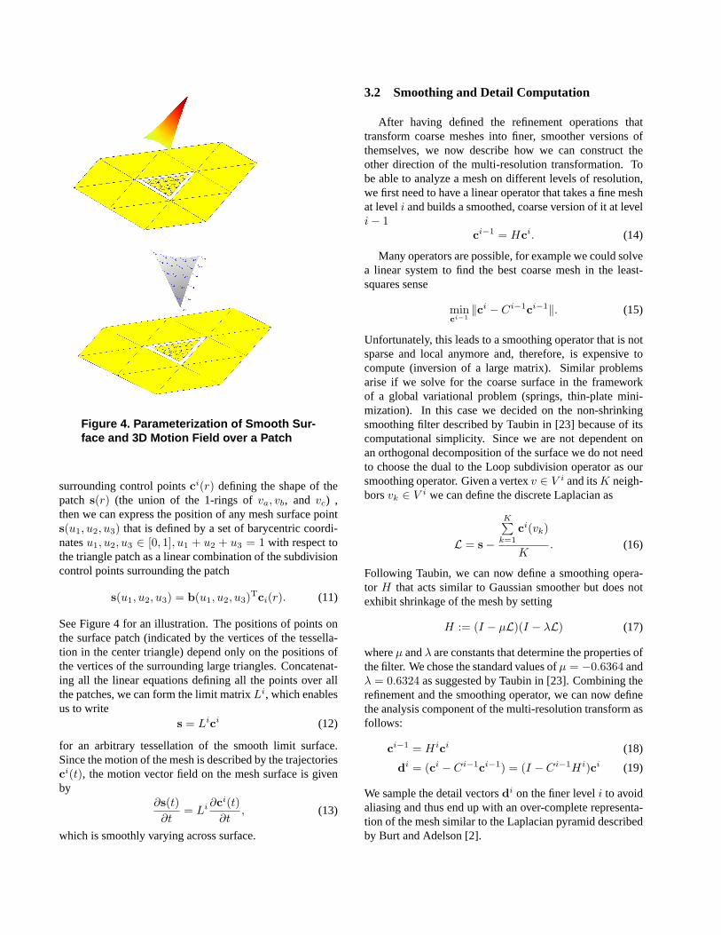
Figure 4. Parameterization of Smooth Sur-face and 3D Motion Field over a Patch

surrounding control pointsci(r) defining the shape of thepatch s(r) (the union of the 1-rings ofva, vb, and vc) ,then we can express the position of any mesh surface points(u1, u2, u3) that is defined by a set of barycentric coordi-natesu1, u2, u3 ∈ [0, 1], u1 + u2 + u3 = 1 with respect tothe triangle patch as a linear combination of the subdivisioncontrol points surrounding the patch

s(u1, u2, u3) = b(u1, u2, u3)Tci(r). (11)

See Figure 4 for an illustration. The positions of points onthe surface patch (indicated by the vertices of the tessella-tion in the center triangle) depend only on the positions ofthe vertices of the surrounding large triangles. Concatenat-ing all the linear equations defining all the points over allthe patches, we can form the limit matrixLi, which enablesus to write

s = Lici (12)

for an arbitrary tessellation of the smooth limit surface.Since the motion of the mesh is described by the trajectoriesci(t), the motion vector field on the mesh surface is givenby

∂s(t)∂t

= Li ∂ci(t)∂t

, (13)

which is smoothly varying across surface.

3.2 Smoothing and Detail Computation

After having defined the refinement operations thattransform coarse meshes into finer, smoother versions ofthemselves, we now describe how we can construct theother direction of the multi-resolution transformation. Tobe able to analyze a mesh on different levels of resolution,we first need to have a linear operator that takes a fine meshat leveli and builds a smoothed, coarse version of it at leveli− 1

ci−1 = Hci. (14)

Many operators are possible, for example we could solvea linear system to find the best coarse mesh in the least-squares sense

minci−1

‖ci − Ci−1ci−1‖. (15)

Unfortunately, this leads to a smoothing operator that is notsparse and local anymore and, therefore, is expensive tocompute (inversion of a large matrix). Similar problemsarise if we solve for the coarse surface in the frameworkof a global variational problem (springs, thin-plate mini-mization). In this case we decided on the non-shrinkingsmoothing filter described by Taubin in [23] because of itscomputational simplicity. Since we are not dependent onan orthogonal decomposition of the surface we do not needto choose the dual to the Loop subdivision operator as oursmoothing operator. Given a vertexv ∈ V i and itsK neigh-borsvk ∈ V i we can define the discrete Laplacian as

L = s−

K∑k=1

ci(vk)

K. (16)

Following Taubin, we can now define a smoothing opera-tor H that acts similar to Gaussian smoother but does notexhibit shrinkage of the mesh by setting

H := (I − µL)(I − λL) (17)

whereµ andλ are constants that determine the properties ofthe filter. We chose the standard values ofµ = −0.6364 andλ = 0.6324 as suggested by Taubin in [23]. Combining therefinement and the smoothing operator, we can now definethe analysis component of the multi-resolution transform asfollows:

ci−1 = Hici (18)

di = (ci − Ci−1ci−1) = (I − Ci−1Hi)ci (19)

We sample the detail vectorsdi on the finer leveli to avoidaliasing and thus end up with an over-complete representa-tion of the mesh similar to the Laplacian pyramid describedby Burt and Adelson [2].

Figure 5. Control Meshes at different Resolu-tions and their detail differences

3.3 Synthesis

This decomposition now leads to the following linearsynthesis algorithm. As described in the section 3.1, oneach leveli, we can express the position of the controlpointsci as a linear combination of the control points ona coarser levelci−1 and the detail coefficientsdi−1 that ex-press the additional degrees of freedom of the vertices in therefined leveli. Formally, we can write

ci = [Ci−1Di][

ci−1

di

]. (20)

Di can be defined in numerous ways, e.g. as the identitymatrix as in Equation 19 or defining a local coordinate sys-tem as in section 3.4.

The decomposition can now be iterated (similar to [16])

ci = [Ci−1Di][

ci−1

di

](21)

= [Ci−1Di][Ci−2 Di−1 0

0 0 Ii

] ci−2

di−1

di

.

and we end up with the following expression that relates thelimit surface linearly to the control pointsc0 of the coarseinitial mesh and the detail coefficientsdj on all levels1 ≤j ≤ i:

s = LiCici∗ (22)

Ci =

i−1∏j=0

Cj ,i−1∏j=1

CjD1,i−1∏j=2

CjD2, . . . , Ci−1Di−1, Di

ci∗ =

[c0,d1,d2, . . .di

]

Figure 6. Detail Encoding in Global and Lo-cal Coordinate Systems

Although we have a nice and simple decomposition thatrelates the motion and shape of the object linearly to the val-ues of the control and detail coefficients, there is a problemwith the approach so far. To achieve a linear representationof the surface in terms of its control vectors, we need toencode the detail level in a global coordinate system. Un-fortunately, this prevents us from optimizing the differentlevels of resolution independently, because changes on acoarse level will cause unintended changes of the global ob-ject shape as can be seen in Figure 6. Most of the differencein shape between successive levels can be represented bya displacement along the normal to the surface as indicatedby the histogram of the magnitudes of the detail coefficientsin Figure 7. This is quite obvious since the discrete Lapla-cian is an approximation of the local normal direction, thusmost of the smoothing in the analysis step occurs parallel tothe surface normal. In summary, most of the characteristicshape information is encoded along the local normal direc-tions and during the synthesis step the local detail shouldbe added back relative to the local coordinate frame to takeadvantage of this and to decorrelate the different levels ofresolution. If we were just interested in shape estimation,this would also suggest to take advantage of local encodingto reduce the dimensionality of our estimation problem byrestricting the detail vectors to vary only along the normal

Figure 7. Histogram encoding the magni-tude of the normal (black) and tangential(gray,white) components of the detail vec-tors in the multi-resolution encoding of themesh

directions. Unfortunately, since we are also interested inmotion estimation we need the tangential component of thelocal encoding to be able to represent the part of the motionfield parallel to the tangent plane of the surface.

A local encoding of the detail vectors is especially im-portant in the case of motion estimation, because if we havea motion that is well described by the trajectories of the con-trol vectors on a coarser level, then the trajectories of thelocally encoded detail coefficients will not need to be ad-justed. An example would be the encoding of a moving armincluding a detailed hand that it is not moving relative to thearm. If we encode the fingers in a global coordinate system,we would get large changes in the detail coefficients to beable describe the motion of the fingers. If we have a localencoding, we just need to add the local shape details to therefined control mesh on the coarser level that was moved bythe global motion of the arm and we the new shape is ac-curately synthesized since the local frames moved with theglobal motion.

3.4 Encoding of Detail in Local Frames

To define the detail coefficients with respect to a localframe, we apply two linear operatorsR andQ to the con-trol meshci that result in two linearly independent vec-tors ri(v) = (Rci)(v) andqi(v) = (Qci)(v) in the tan-gent plane tos(v). We can use them to define a local or-thonormal frame atv F i(v) = (ni(v), ri(v),qi(r)) whereni(v) = ri(v) × qi(r). Details about how to define theseoperators in the case of the Loop subdivision scheme can befound in Hoppe [7].

Including the local encoding in our multi-resolution

Figure 8. Flow chart describing the multi-resolution analysis and synthesis

framework, we summarize the steps of the transform (fora graphical flow chart see Figure 8)

ANALYSIS:

for i = n:-1:1di = (F i)T(I − SH)ci

ci−1 = Hci

end

SYNTHESIS:

for i = 1:nci = Sci−1 + (F i)di

ends = Lncn

This forms the basis of our multi-resolution algorithm.Given a decomposition of our shape estimate into the dif-ferent levels of resolution, the detail coefficients are mod-ified one level at a time. If we do not have a shape esti-mate yet, we start from a coarse meshc0 with few verticesand set all the detail coefficients to zero. The estimationof the spatio-temporal structure is always done bottom up,decomposition level by decomposition level. When opti-mizing detail coefficients on leveli, we compute the valueof ci−1 using the coarse base meshc0 and the detail levelsdj 1 ≤ j ≤ i − 1. This also determines the local frameF i−1. The changes in the detail coefficients are then prop-agated to the mesh surface by continuing the synthesis pro-cedure, and then we can evaluate the error measure. Afterthe optimization converges or a fixed number of iterations

Figure 9. Silhouette Intersection

has been applied, we precomputeci using our estimate ofdi and continue to optimize overdi+1, thereby increasingthe degrees of freedom of the mesh. This is continued untilwe reach the maximum refinement depth. The refinementcan be locally controlled by the magnitude of the detail co-efficients. If they are small in a region of the mesh, there isno need for further subdivision. This enables the algorithmto adapt the mesh resolution according to the complexity ofthe surface geometry.

4 Multi-Camera Shape and Motion Estima-tion

The shape and motion estimation can be subdivided intotwo different parts. Initially, we do not know anything aboutour object except that it is located somewhere inside the vol-ume observed by the cameras (which may see only parts ofthe object at any given time) and that the object is mov-ing (if it is not moving then we need background imagesto distinguish the object from the background). Thus, thefirst step of the algorithm tries to locate the object of inter-est in the working volume, and estimate an approximationto its shape as well as motion. Having an initial estimateof the spatio-temporal structure of the object, we then applyour multi-resolution optimization framework to the struc-ture using stereo constraints.

4.1 Shape Initialization

The shape initialization is based up on a subdivision ofthe working volume into voxels, which are then projected

Figure 10. Image Silhouettes

into all the images. We then accumulate the evidence forthe voxel being inside or outside the object. The evidenceis defined in Eq. 23 as the ratio between the temporal imagegradient and the local spatial gradient (λ is a small positiveconstant to ensure a well-defined measure everywhere):

θ(P) =∑

k∈Cameras

θk(P) =∂I(pk)

∂t

λ + ‖∇I(pk)‖2(23)

For each image the ratiosθi(P) are formed by integratingover the footprint of the voxel corresponding to the 3D lo-cationP (see Figure 10 for two examples of the thresholdedimages of ratios). If the assumption of a moving object is vi-olated, we can also incorporate the difference between theimage sequence and previously recorded background im-ages into the algorithm. The voxel volume is smoothedand thresholded using 3D morphological filters, before aniso-surface extraction algorithm determines the initial shapeand topology of the mesh. Given an iso-surface, we thenconvert it into a base mesh with subdivision connectivityusing the following algorithm:

1. Simplify the triangle mesh representation down to acoarse base resolution

2. Displace the vertices of the subdivision mesh alongtheir surface normal direction until they lie on the iso-surface

3. Refine the mesh as described in Section 3.1

4. Repeat this process until the subdivision mesh approx-imates the iso-surface well.

Using a voxel algorithm based on the intersection of sil-houettes in the images only allows us to find the visualhull [13] of the object in view (Figure 9). For some ap-plications this might be good enough [17], but we wouldlike to capture all the shape and motion detail of the object.

We apply this algorithm to all the frames of the sequencewhich results in an approximation to the shape of the objectat each time instance. Unfortunately, from these shapes wecan only extract the component of the 3D motion that is nor-mal to the object surface, but not the tangential component.Thus to compute the trajectories of the mesh vertices overtime, we need to include image derivative information.

a) b)

Figure 11. 3D Normal Flow

4.2 Motion Initialization

To find the correspondence between vertices over timeand to compute an initial estimate for the 3D motion field,we use the spatio-temporal gradients in the images and re-late them to the motion vectors on the object surface. Fromequation 6 it follows that each normal flow measurement,that is the component of the image flow that is perpendicu-lar to the local brightness gradient in an image, constrainsthe projection of the 3D motion flow to lie along a line par-allel to the iso-brightness contour in the image, the normalflow constraint line. Thus the 3D motion flow vector hasto lie on the plane defined by the normal flow constraintline and the optical center of the camera as shown in Fig-ure 11a. Using the approximation to the shape computedbefore, we intersect the planes of corresponding measure-ments in space. The intersection should ideally be a singleline in space, the 3D normal flow constraint line that is par-allel to the iso-brightness contour on the object. The com-ponent of the 3D motion along the iso-brightness contouris not recoverable. This is the aperture problem revisitedin 3D. Since each control motion vector is constrained bymany samples (see the parameterization of each sample ina patch in Figure 4), and we expect the gradient directionsto vary on the object surface, we can expect the estimationof these motion vectors to be nevertheless well-defined (see11b for an illustration).

Since the shape we use to correspond the measurementsis only an approximation, we can expect to have errors whencorresponding measurements across cameras. To detect badcorrespondences, we compute a measure for the collinear-ity of the intersections between the normal flow constraintplanes and use it to prune bad correspondences.

Taking the derivative of Equation 4 with respect to time,

and substituting it into equation 6, we can define the follow-ing linear constraint at each sample pointP = s(u1, u2, u3)on the object surface patchr:

−∂I(pk)∂t

= ∇I(pk)T · dpk

dt(24)

= ∇I(pk)> · ∂pk

∂P∂P∂t

= ∇I(pk)> · ∂pk

∂P∂s(u1, u2, u3)

∂t

= ∇I(pk)> · ∂pk

∂PLn(P)Cn(P)

∂cn∗ (P)∂t

where Ln(P)Cn(P)cn∗ (P) are the components of equa-

tion 22 corresponding to surface pointP. Choosing thedetail refinement matricesDi to be the local frame matri-cesF i corresponding to the current control vector valuesci 1 ≤ i ≤ n, we can define a large linear system by stack-ing all the equations 24. This linear system can now besolved for the derivative of the base control and detail vec-tors with respect to time. These estimated temporal deriva-tives together with the our mesh approximations form anestimate for the trajectories of the control and detail vec-tors. We use a preconditioned conjugate gradient algorithmto solve this overdetermined linear system which convergesalways in a few iterations.

4.3 Shape and Motion Refinement throughSpatio-Temporal Stereo

To refine our estimate of the spatio-temporal surface thatdescribes the object, we adapt the vertex trajectories of themesh, such that a multi-view stereo criterion is optimized.

We assume as expressed in equation 5 that the bright-ness of the projection ofP, that is the pixel value, is sim-ilar across cameras up to a linear transformation and thatis only changing slowly over time. Combining both con-stancy constraints, we have that the similarity between thespatio-temporal volumes that each patchr on the object sur-face traces out in the spatio-temporal image space of eachcamera can be used as a measure for the correctness of ourshape and motion estimation.

To evaluate the error measure, we choose a regular sam-pling pattern inside each surface patch, where the samplingdensity is adjusted per patch in such a way that we haveapproximately one sampling point per pixel in the highestresolution image the patch is visible in. The visibility ofeach patch is determined by a z-buffer algorithm and wedenote the set of camera pairs that mutually see a patch onthe object surface byV(r). Using the subdivision frame-work presented in section 3, we synthesize the shape at anumber of consecutive time instances based on the currentvalues of the base control and detail vectors and evaluate

the following matching functional in space-time based onnormalized correlation

E(r, t) =∑

(i,j)∈V(r)

W(i, j)

t+∆t∫t−∆t

〈Ii(s), Ij(s)〉|Ii(s)| · |Ij(s)|

ds

(25)

+∑

i

t+∆t∫t−∆t

〈Ii(t), Ii(s)〉|Ii(t)| · |Ii(s)|

ds

〈Ii(t), Ij(t)〉 =∫

P∈r

˜Ii(pi(P, t)) · ˜Ij(pj(P, t))dP

˜Ii(pi(P, t)) = Ii(pi(P, t))− Ii(t)

Ii(t) =∫

P∈r

Ii(pi(P, t))dP

|Ii(t)|2 = 〈Ii(t), Ii(t)〉

to compare corresponding spatio-temporal image volumesbetween pairs of cameras. For each sampling point on themesh surface, we determine the intensity values by bilinearinterpolation from the images.

We combine the correlation scores from all the camerapairs by taking a weighted average with the weightsW(i, j)depending on the angles between optical axes of camerasiandj and the surface normal at pointP. Notice that eachvertexv ∈ V i influences the shape only in those patchesthat involve vertices that are part ofv’s 2-ring (vertices thatare at most 2 edges away). We will denote this set of patchesbyT2(v). Thus, when we want to compute the derivatives ofthe error function with respect to the control points, we onlyneed to evaluate the changes of the error measure onT2(v).Due to the non-linearity that was introduced by the localencoding of the detail, we cannot the express the changeof the surface directly as a linear function of the change inthe detail coefficients, but have to synthesize the change onthe surface as described in Figure 8. Since we only haveto evaluate the changes on small patches of the object sur-face at a time, this can be done efficiently though. The finalderivative can then be computed easily using the chain rulefrom the derivative of the projection equation (Eq. 4) andthe spatio-temporal image derivatives.

We use the BFGS-quasi newton method in MATLABTM

Optimization Toolbox to optimize over the control point po-sitions. The upper bounds for their displacement is given bythe boundaries of the voxel volume, which we include as in-equality constraints in the optimization.

So far we have only applied our algorithm on objectsconsisting only of one component, but if the initial shapeapproximation consists of several disconnected parts, wecould use the distance between the disconnected parts tomerge or separate the recovered surfaces. Then we can ap-

Figure 12. Example Input Views

ply the refinement algorithm to every object in turn, whileupdating the visibility globally.

5 Results

We have established in our laboratory a multi-cameranetwork consisting of sixty-four cameras, Kodak ES-310,providing images at a rate of up to eighty-five frames persecond; the video is collected directly on disk. The camerasare connected by a high-speed network consisting of six-teen dual processor Pentium 450s with 1 GB of RAM eachwhich process the data.

For our experiments we used eleven cameras, 9 grayscale and 2 color, placed in a dome-like arrangement aroundthe head of a person (Figure 2) who was opening his mouthto express surprise (example images in Figure 12) andblinking his eyes while turning his head and moving it for-ward.

The recovered spatio-temporal structure enables us tosynthesize texture-mapped views of the head from arbitraryviewing directions (Figures 13a-13c). The textures, com-ing always from the least oblique camera with respect to agiven mesh triangle, were not blended together to illustratethe good agreement between adjacent texture region bound-aries (note the agreement between the grey-value structuresin Figure 13c despite absolute grey-value differences). Un-fortunately, we did not have access to a laser range scan togenerate ground-truth for the shape, but we believe the re-covered control meshes in Figures 13d-13f show that de-spite some artifacts near the eyes the spatial structure ofthe head was recovered well. For a full view of the recon-struction, please see the accompanying videos at the websitewww.videogeometry.com. Since only two cameras werecolor, we were only able to texture map parts of the head incolor.

(a) (b)

(c) (d)

(e) (f)

Figure 13. Results of 3D Structure and Motion Flow Estimation: Structure.(a-c) Three Novel Viewsfrom the Spatio-Temporal Model (d) Left View of Control Mesh (e) Right Side of Final Control Mesh(f) Close Up of Face

(a) (b)

(c) (d)

(e) (f)

Figure 14. Results of 3D Structure and Motion Flow Estimation: Motion Flow. (a-c) Magnitude ofMotion Vectors at Different Levels of Resolution (d) Magnitude of Non-Rigid 3D Flow Summed overthe Sequence (e) Non-Rigid 3D Motion Flow (f) Non-Rigid Flow Close Up of Mouth

Examining the 3D motion fields at different resolutionswe see that the multi-resolution representation is seperatingthe motion field into different components. In Figures 14a-14d we encoded the magnitude of the motion vectors onthe object surface as brighntess values that vary from brightfor large displacements to dark for small displacements.The brightness values are increasing proportionally with themagnitude of the motion energy. Figure 14a shows that atthe coarsest level the magnitudes of the 3 flow vectors varylittle across the object, which is to be expected since the tra-jectories on the coarsest level should encode the rigid mo-tion of the object. At next finer level (Figure 14b) we seethat most of the motion energy is concentrated in the eyeand motion region which corresponds well to the activityin the scene. Further increasing the scale, we notice thatthe magnitude of the motion vectors concentrates more andmore at only a few places (Figure14c), in this example thefast blinking motion of the eye is the prominent motion.

To separate the non-rigid 3D motion flow of the mouthgesture from the motion field caused by the turning of thehead, we fit a rigid flow field to the trajectories of thecoarsest mesh levelc0 by parameterizing the 3D motionflow vectors by the instantaneous rigid motion∂c0/∂t =v + ω × c0, wherev andω are the instantaneous trans-lation, and rotation ([8]). By subtracting the rigid motionflow from the full flow, we extract the non-rigid flow. Itcan be seen that the motion energy (integrated magnitudeof the flow over the whole sequence) is concentrated in thenon-rigid regions of the face such as the mouth and the jawas indicated by the higher brightness values in Figure 14d.In contrast, the motion energy on the rigid part of the head(e.g., forehead, nose and ears) is significantly smaller. Inthe close up view of the mouth region (Figure 14f) we caneasily see, how the mouth opens, and the jaw moves down.Although, it is obviously hard to visualize dynamic move-ment by static imagery, the vector field and motion energyplots (Figure 14) illustrate that the dominant motion – theopening of the mouth – has been correctly estimated.

6 Conclusion and Future Work

To conclude, we presented a method that is able to re-cover an accurate 3D spatio-temporal description of an ob-ject by combining the structure and motion estimation ina unified framework. The technique can incorporate anynumber of cameras and the achievable depth and motionresolution depends only on the available imaging hardware.

In the future, we plan to explore other surface represen-tations where we are able to adapt not just the geometry,but also the connectivity (see [11]) according the some op-timization criterion. It is also interesting to study the con-nection between multi-scale mesh representation and multi-scale structure of image sequences that observe them to in-

crease the robustness of the algorithm even further by im-proving the stopping criteria for the mesh refinement andthe optimization.

One important issue for the 3D structure and motionestimation problem is the absence of good benchmark se-quences including ground truth data. Due to the technicaldifficulties involved in the capture and calibration of thesesequences, there are only very few sequences available forprocessing right now. We hope that in the future a bench-mark data collection will evolve, so that we will be able tocompare our algorithms on a standard data set against otherresearcher’s algorithms as it is customary for the stereo oroptical flow problem.

References

[1] J. S. D. Bonet and P. Viola. Roxels: Responsibility weighted3d volume reconstruction. InProceedings of ICCV, Septem-ber 1999.

[2] P. Burt and E. H. Adelson. The laplacian pyramid as a com-pact image code.IEEE Transactions on Communication, 31,1983.

[3] R. L. Carceroni and K. Kutulakos. Multi-view scene cap-ture by surfel sampling: From video streams to non-rigid 3dmotion, shape, and reflectance. InProc. International Con-ference on Computer Vision, June 2001.

[4] I. Essa and A. Pentland. Coding, analysis, interpretation,and recognition of facial expressions.IEEE Trans. PAMI,19:757–763, 1997.

[5] O. Faugeras and R. Keriven. Complete dense stereovisionusing level set methods. InProc. European Conference onComputer Vision, pages 379–393, Freiburg, Germany, 1998.

[6] P. Fua. Regularized bundle-adjustment to model heads fromimage sequences without calibration data.InternationalJournal of Computer Vision, 38:153–171, 2000.

[7] H. Hoppe, T. DeRose, T. Duchamp, M. Halstead, H. Jin,J. McDonald, J. Schweitzer, and W. Stuetzle. Piecewisesmooth surface reconstruction. InProc. of ACM SIG-GRAPH, pages 295–302, 1994.

[8] B. K. P. Horn.Robot Vision. McGraw Hill, New York, 1986.[9] A. Hubeli and M. Gross. A survey of surface representations

for geometric modeling. Technical Report 335, ETH Zurich,Institute of Scientific Computing, March 2000.

[10] I. Kakadiaris and D. Metaxas. Three-dimensional humanbody model acquisition from multiple views.InternationalJournal of Computer Vision, 30:191–218, 1998.

[11] L. Kobbelt, T. Bareuther, and H.-P. Seidel. Multiresolutionshape deformations for meshes with dynamic vertex connec-tivity. In Eurographics 2000 proceedings, 2000.

[12] K. N. Kutulakos and S. M. Seitz. A theory of shape by spacecarving. International Journal of Computer Vision, 38:199–218, 2000.

[13] A. Laurentini. The visual hull concept for silhouette-basedimage understanding. IEEE Trans. PAMI, 16:150–162,1994.

[14] C. Loop. Smooth subdivision surfaces based on triangles.Master’s thesis, University of Utah, 1987.

[15] S. Malassiotis and M. Strintzis. Model-based joint motionand structure estimation from stereo images.Computer Vi-sion and Image Understanding, 65:79–94, 1997.

[16] C. Mandal, H. Qin, and B. Vemuri. Physics-based shapemodeling and shape recovery using multiresolution subdivi-sion surfaces. InProc. of ACM SIGGRAPH, 1999.

[17] W. Matusik, C. Buehler, S. J. Gortler, R. Raskar, andL. McMillan. Image based visual hulls. InProc. of ACMSIGGRAPH, 2000.

[18] R. Plankers and P. Fua. Tracking and modeling people invideo sequences.International Journal of Computer Vision,81:285–302, 2001.

[19] P. Schroder and D. Zorin. Subdivision for modeling andanimation. Siggraph 2000 Course Notes, 2000.

[20] S. Seitz and C. Dyer. Photorealistic scene reconstruction byvoxel coloring. International Journal of Computer Vision,25, November 1999.

[21] H. Spies, B. Jahne, and J. Barron. Regularised range flow. InProc. European Conference on Computer Vision, June 2000.

[22] J. Stam. Evaluation of loop subdivision surfaces. SIG-GRAPH’99 Course Notes, 1999.

[23] G. Taubin. A signal processing approach to fair surface de-sign. InProc. of ACM SIGGRAPH, 1995.

[24] S. Vedula, S. Baker, P. Rander, R. Collins, and T. Kanade.Three-dimensional scene flow. InProc. InternationalConference on Computer Vision, Corfu,Greece, September1999.

[25] S. Vedula, S. Baker, S. Seitz, and T. Kanade. Shape andmotion carving in 6d. InProc. IEEE Conference on Com-puter Vision and Pattern Recognition, Head Island, SouthCarolina, USA, June 2000.

[26] S. Vedula, P. Rander, H. Saito, and T. Kanade. Modeling,combining, and rendering dynamic real-world events fromimage sequences. InProc. of Int. Conf. on Virtual Systemsand Multimedia, November 1998.

[27] Y. Zhang and C. Kambhamettu. Integrated 3d scene flowand structure recovery from multiview image sequences. InProc. IEEE Conf. Computer Vision and Pattern Recognition,pages II:674–681, Hilton Head, 2000.

[28] D. Zorin, P. Schrder, and W. Sweldens. Interactive multires-olution mesh editing. InProc. of ACM SIGGRAPH, 1997.