Specifying uncertainty for mobile robots?

Mathijs de Weerdt, Frank de Boer, Wiebe van der Hoek and John-Jules MeyerUtrecht Universitymmweerdt@cs.uu.nl, frankb@cs.uu.nl, wiebe@cs.uu.nl, jj@cs.uu.nl9th October 1998

Contents1 Autonomous mobile robots 51.1 Introduction . . . . . . . . . . . . . . . . . . . . . . . . . . . . . . . . . . . . . 51.2 Map building . . . . . . . . . . . . . . . . . . . . . . . . . . . . . . . . . . . . 61.3 Localization . . . . . . . . . . . . . . . . . . . . . . . . . . . . . . . . . . . . . 61.4 Obstacle avoidance, planning and control . . . . . . . . . . . . . . . . . . . . 71.5 Agent Oriented Programming . . . . . . . . . . . . . . . . . . . . . . . . . . . 71.6 The Bayesian method . . . . . . . . . . . . . . . . . . . . . . . . . . . . . . . 81.7 Di�erent sources of uncertainty . . . . . . . . . . . . . . . . . . . . . . . . . . 92 Various ways of map building 112.1 Fuzzy methods . . . . . . . . . . . . . . . . . . . . . . . . . . . . . . . . . . . 112.1.1 Map building . . . . . . . . . . . . . . . . . . . . . . . . . . . . . . . . 112.1.2 Localization by coincident boundaries . . . . . . . . . . . . . . . . . . 152.1.3 Localization by approximate locations . . . . . . . . . . . . . . . . . . 162.2 Occupancy maps . . . . . . . . . . . . . . . . . . . . . . . . . . . . . . . . . . 162.2.1 A certainty grid . . . . . . . . . . . . . . . . . . . . . . . . . . . . . . 162.2.2 Position probability grid . . . . . . . . . . . . . . . . . . . . . . . . . . 172.2.3 An evidential approach . . . . . . . . . . . . . . . . . . . . . . . . . . 172.3 Saphira . . . . . . . . . . . . . . . . . . . . . . . . . . . . . . . . . . . . . . . 193 Logics for mobile robots 213.1 A logic-based framework . . . . . . . . . . . . . . . . . . . . . . . . . . . . . . 213.2 Situation calculus . . . . . . . . . . . . . . . . . . . . . . . . . . . . . . . . . . 223.3 Modal logic . . . . . . . . . . . . . . . . . . . . . . . . . . . . . . . . . . . . . 233.3.1 A logic of belief . . . . . . . . . . . . . . . . . . . . . . . . . . . . . . . 233.3.2 Adding probability . . . . . . . . . . . . . . . . . . . . . . . . . . . . . 243.4 The KARO-framework . . . . . . . . . . . . . . . . . . . . . . . . . . . . . . . 254 Uncertainty speci�ed by a probabilistic modal logic 274.1 Introduction . . . . . . . . . . . . . . . . . . . . . . . . . . . . . . . . . . . . . 274.2 Speci�cation of the language . . . . . . . . . . . . . . . . . . . . . . . . . . . 274.2.1 The basic language . . . . . . . . . . . . . . . . . . . . . . . . . . . . . 284.2.2 The basic model . . . . . . . . . . . . . . . . . . . . . . . . . . . . . . 284.3 Adding actions: Dynamic logic . . . . . . . . . . . . . . . . . . . . . . . . . . 334.3.1 Extension to the language . . . . . . . . . . . . . . . . . . . . . . . . . 334.3.2 Modi�cations to the Kripke model . . . . . . . . . . . . . . . . . . . . 343

4 CONTENTS4.4 Application: Simplebot in a linear world . . . . . . . . . . . . . . . . . . . . 364.4.1 An example . . . . . . . . . . . . . . . . . . . . . . . . . . . . . . . . . 364.4.2 Incorporating the observe action in our language . . . . . . . . . . . 384.4.3 Incorporating a move action in our language . . . . . . . . . . . . . . 454.5 The two-dimensional world . . . . . . . . . . . . . . . . . . . . . . . . . . . . 554.5.1 Linear sonar beam . . . . . . . . . . . . . . . . . . . . . . . . . . . . . 574.5.2 Sonar segment . . . . . . . . . . . . . . . . . . . . . . . . . . . . . . . 594.5.3 Move and turn . . . . . . . . . . . . . . . . . . . . . . . . . . . . . . . 604.6 Implementation . . . . . . . . . . . . . . . . . . . . . . . . . . . . . . . . . . . 614.6.1 Probability maps . . . . . . . . . . . . . . . . . . . . . . . . . . . . . . 614.6.2 A Pioneer in the real world . . . . . . . . . . . . . . . . . . . . . . . . 655 Discussion and future work 695.1 Comparing to related work . . . . . . . . . . . . . . . . . . . . . . . . . . . . 695.2 Discussion . . . . . . . . . . . . . . . . . . . . . . . . . . . . . . . . . . . . . . 705.3 Future research . . . . . . . . . . . . . . . . . . . . . . . . . . . . . . . . . . . 70

Chapter 1Autonomous mobile robots1.1 IntroductionNowadays many arti�cially intelligent systems are being used. Entities like this, which areautonomous and able to take actions, are called agents. These agents are used for a lot ofdi�erent tasks and their area of applications is still expanding. With more and more agentsbeing used in sensitive applications, as medicine and tra�c control, the importance of beingable to reason about their behavior increases. Therefore, several logics are being studied.Especially modal logics are powerful tools to do this reasoning. It may also be possible to usethese tools not only to reason about the agent's behavior, but also to actually perform thereasoning by the agent.A special case of an agent is a mobile robot. A mobile robot is an object which is ableto move, has some way of observing its environment and is able to perform some reasoningabout its observations. `Robot' is Czech for someone who is forced to work, but now it'sused to describe complicated and sometimes man-like machines. If such a mobile robot candecide where to go by itself, it is called an autonomous mobile robot. We will describe variousexisting methods to add a reasoning mechanism and some rules about how to change its modelof the world to a robot, making it truly autonomous. This mechanism has to make a map ofthe environment, localize the robot in this environment and plan where it should go to.In this document we will use the term robot to denote an autonomous mobile robot. So,all robots in this documents are agents because they are autonomous. In general many robotsexist in for example factories, which are not autonomous robots and therefore not agents.Most of these robots are controlled by a human or just execute a preprogrammed sequence ofactions. Only a small amount of robots found in factories are really able to take decisions andexecute action on their own and thus are truly autonomous, but this number is increasingvery fast.This document is arranged as follows. First, we will introduce three parts of the reasoningmechanism. Then we will introduce some other important concepts concerning autonomousmobile robots, for example di�erent sources of uncertainty. In the next chapter we willsummarize some existing map-building and localization methods and in chapter 3 we willdescribe some methods for specifying uncertainty.The main topic of the research leading to this document is to �nd out how modal logic canbe used to describe the uncertainty introduced by the sensors of mobile robots. Learning fromthe work described in these two chapters, we developed a language which is able to deal with5

6 CHAPTER 1. AUTONOMOUS MOBILE ROBOTSboth uncertainty and actions. We will introduce this language in chapter 4. Accompaniedwith many simple examples we will extend the presented model step by step to suit it forrather realistic robots and environments. In the last chapter this model will be compared tothe existing ones and some directions will be given for future research.1.2 Map buildingA mobile robot has some way of observing its environment. We call the tools to collectdata from the environment sensors. The most common sensors, like sonars and laser-beamsdetect the distance to an obstacle within the range of the sensor by sending out a signaland measuring the time till the echo of the signal returns. In most occasions the signal willbounce against the nearest obstacle in the direction of the sensor and therefore the measureddistance will be the distance to the nearest obstacle. Unfortunately, the returned distancecan be signi�cantly di�erent from the real distance to the nearest obstacle. The many causesfor such failures are summarized in section 1.7.We would like to create a map of the environment from the observations done by thesensors. Suppose the agent knows its starting position and receives a stream of sensor dataconcerning the distance to the nearest obstacle in certain directions. All these data can bedrawn as points in a plane. Points very close together can be joined by a line representing asmall piece of a wall or the vertex of some object.Suppose the robot has some way to measure its own position relative to its startingposition. Most robots are able to calculate the distance and direction travelled from observingthe way the left and right wheel turn. This process is called dead reckoning. Then the robotcan move and update its position and orientation in the map. New observations can be drawnrelative to its new location. In this way a map of the environment can be built.Unfortunately, not only the observed distances to obstacles can be very erroneous, alsothe dead reckoning process can introduce errors. To build a map that is at least a bit reliable,as many of the sources of uncertainty and noise as possible has to be accounted for. Thecomplete method of �ltering observations and combining them to lines or objects in a map iscalled map building.1.3 LocalizationAs we said in the previous section, the robot is able to calculate its position relative to its startposition, but this new position is not exact. The deviation of this derived position comparedto the real relative position accumulates while moving and after a few displacements crossesall acceptable limits. If the robot already has a partial map of the environment, it may beable to correct this accumulated dead reckoning errors. This process is called localization.In general, localization works as follows. Next to the global map, the robot also constructsa local map. New observations are only added to the local map. The local map is matchedto the global map around the current estimated position. If a match is found, the positionis adjusted and the new observations in the local map are transferred to the global map. Ifnot, the robot just keeps on going. In section 2.1.2 and 2.1.3 some di�erent versions of thisprocess are described more detailed.The methods which assume the robot is near its estimated position are run in parallelwith other processes to update this position. These methods solve a problem called the dead-

1.4. OBSTACLE AVOIDANCE, PLANNING AND CONTROL 7reckoning or position-tracking problem. Some methods are able to derive the robot's positionwithout any estimated position. For example, this is needed when the robot already has amap of the environment, but has been turned o�. Then it should try to �nd out where it is.These algorithms can also be used when the position-tracking method fails.1.4 Obstacle avoidance, planning and controlIn order to let an agent or robot behave intelligible, it should plan its actions based onits knowledge of the environment and of its goals. A large part of this process is aboutmotion planning, which is described in the following subsection. However, just planning themovements of the robot based on its knowledge of the environment is not enough. In the realworld, strange things may happen, like human beings jumping in front of the robot (to seewhether it stops). Therefore another process has to run concurrently to ensure a last-minuteavoidance of previously unknown obstacles. This process is called an obstacle avoidancebehavior and is far more low-level than the global planning.Some control systems consists only of behaviors like obstacle avoidance. In fact, most ofthe example programs of Saphira [KMRS97] just consists of these basic behaviors.Motion planningGiven a goal location, motion planning is the process that decides, using the current imageof the environment, which route to take to reach this goal. In general this problem is ratherdi�cult, because a robot has a certain shape and a limited ability to turn and move concur-rently. The problem is not that hard if the robot is just a point. Therefore, this problem istackled by �rst transforming the map of the environment into a con�guration space.Each point in the con�guration space represents an orientation and a location of the centerof the robot. Combinations of locations and orientations near obstacles in the map which areimpossible, become con�guration `obstacles'. The dimension of the con�guration space is atleast one higher than the dimension of the original map, because of the possible directionsthe robot can turn to. The new problem is to �nd a route through this higher-dimensionalspace without cutting any `obstacles'. Many variants of this problem have been solved in the�eld of robotics and computional geometry [Lau98] or by using the theory of Markov decisionprocesses [KLC98].In this document we focus on applying a logic which is able to specify uncertainty, beliefand the results of actions to map-building. Brafman c.s. have described the use of a logicof knowledge and time to state sound and complete termination conditions in the motionplanning domain [BLMS97], but they did not incorporate probabilities in their language.1.5 Agent Oriented ProgrammingIn many articles about agents a method called AOP is mentioned. AOP is short for agentoriented programming and is a specialization of the very popular design method called objectoriented programming. During the ICMAS'98 Jacques Ferber explained the development ofdi�erent programming paradigms like these two very clearly, see �gure 1.1. The ideas aboutnavigation and planning of mobile agents have to be implemented and it is very useful tocheck whether someone already has made some kind of a framework.

8 CHAPTER 1. AUTONOMOUS MOBILE ROBOTS

atomsassemblerprocedures and functionsobjects distributed objectsmobile objectsautonomous agentsmulti-agent systemscells animals organisational societiesFigure 1.1: Software design levels and their biological equivalents.The AOP framework consists of three primary components. First, we have a formallanguage with a clear syntax and semantics to describe a mental state. This mental state isde�ned uniquely by several modalities such as belief and commitment. The second componentis a programming language in which the agents are programmed, with primitive request andinform commands. The semantics of the programming language will depend in part on thesemantics of the mental state. And �nally, such a framework consists of a method to convertneutral devices into programmable agents.This document does not pay much attention to the programming and design problems,but before starting to implement, one should take a look at an overview of agent orientedprogramming methods [Sho93].1.6 The Bayesian methodIn this document we use probabilities to describe uncertainty. Some of them are conditionalprobabilities. These are probabilities of a certain event knowing that something else alreadyhas happened. Bayes' theory is used to reason about such conditional probabilities. Thedetails of this theory are covered by the �rst part of section 4.4.2.The main part of this theory is Bayes' rule. If we take a collection of statements B1; : : : ; Bnof which always precisely one is true, we can calculate the probability for each of thesestatements under the condition of some other statement A as follows:PfBj jAg = PfAjBjg � PfBjgPi PfAjBig � PfBig (1.1)This rule can be used to calculate a conditional probability using other conditional proba-bilities. For example we have a robot at position 0 in a world of size 10 and the statements\the nearest obstacle is at position x" for x = 1; : : : ; 10. The initial probabilities for thesestatements are 0:1. Suppose the robot would like to know the probability that the nearestobstacle is at distance 2, knowing that it just has observed that the distance to the nearest

1.7. DIFFERENT SOURCES OF UNCERTAINTY 9obstacle is 3. This can be calculated as follows:Pfnearest obstacle(2)jobserved(3)g == Pfobserved(3)jnearest obstacle(2)g�Pfnearest obstacle(2)gPi=1;:::10Pfobserved(3)jnearest obstacle(i)g�Pfnearest obstacle(i)g == Pfobserved(3)jnearest obstacle(2)g�0:1Pi=1;:::10Pfobserved(3)jnearest obstacle(i)g�0:1 (1.2)We still need to de�ne the conditional probabilities that the robot observes 3 while the nearestobstacle is at distance i. We could use a discrete normal distribution like this one:Pfobserved(y)jnearest obstacle(x)g = approxnormal(x� y)approxnormal(i) = 8>>><>>>: if i = �1 then 0:25if i = 0 then 0:5if i = 1 then 0:25otherwise 0:0 (1.3)The result of equation (1.2) with this de�nition will be:Pfnearest obstacle(2)jobserved(3)g = 0:25 � 0:1(0:25 + 0:5 + 0:25) � 0:1 = 0:25 (1.4)So, to use this rule a lot of conditional probabilities have to be de�ned in advance. Forexample, we de�ned the probability that the robot observes that the distance to this obstacleis y, while we know that the obstacle is at distance x. This is one of the major disadvantagesof this approach, although in our case, it is possible to experimentally establish this function.The other problems using this approach are that the several conditions (like \the distance tothe nearest obstacle is 3") must be disjunct and the sum of their probabilities must be one.The result of a method using Bayes' rule depends also on the quality of the de�nitions ofthe conditional probabilities. Since some authors feel that it is not possible to de�ne theseprobabilities well enough, they refrain from using probabilities and Bayes' theory, but use forexample fuzzy logic.1.7 Di�erent sources of uncertaintyBefore starting to develop a complicated system to deal with uncertainty and noise concerningmobile robots, we �rst investigate what the di�erent sources of this uncertainty are. Thesesources are slightly di�erent for di�erent kinds of sensors. We assume the robot has sonarsor sensors like the ones we described in section 1.2. The map built by a robot can containmany errors, because of the following reasons:� Prior knowledge about the environment may be incorrect, for example because mapsomit details and temporary features, spatial relations may have changed and the metricinformation in the map may be imprecise.� Perceptually acquired information is unreliable, because{ this information is in uenced by environmental features like occlusion and specularre ection,{ the sensors have only a limited range,

10 CHAPTER 1. AUTONOMOUS MOBILE ROBOTS

Figure 1.2: If the surface is very smooth, the sound will re ect like a mirror re ects light.This is called specular re ection.{ the accuracy is often dependent on the angle between the direction of the sensorand the boundary of the obstacle,{ di�erent surface properties result in di�erent results, for example if the surface isvery smooth, the sound will re ect like light in a mirror, see �gure 1.2,{ the result depends on where in the beam the re ection was,{ the accuracy of the results is in uenced by the distance between the sensor andthe object,{ the ambient temperature and air turbulence in uence the time of ight, if it is veryhot, it takes somewhat longer for sound to travel through the air,{ adverse observation conditions like poor lighting lead to noisy data,{ and the wheel encoders have some inaccuracy.� The e�ect of control actions is not completely reliable. Wheels may slip and the grippermay lose its grasp on the object.� Errors in the measurement interpretation may lead to incorrect beliefs. Take for examplea situation in which the signal does not re ect to the robot itself, because of the relativeangle of the surface. If the robot stands still for some time at this place, the same erroris made all the time, but the robot might become more and more sure of the correctnessof its observations [Kon96].� Real-world environments have unpredictable dynamics. Objects move or the environ-ment is changed by other agents, even relatively stable features may change over time,think for example of seasonal changes.Not all of these causes can be accounted for, but the approaches in the next chapter tryto take care of as many of them as possible.

Chapter 2Various ways of map buildingIn this chapter we describe a couple of existing map building methods. All these methodshave been implemented by their respective authors and seem to work rather well. Thesemethods can be divided into at least two groups. First, we describe two methods whichmake an extensive use of fuzzy logic, thereafter we explain two methods using a probabilisticapproach. Finally, we describe shortly the package Saphira delivered with the Pioneers,medium sized mobile robots from Real World Interface [Int], which includes several di�erentmethods.2.1 Fuzzy methodsIn this section a couple of methods are presented which use fuzzy logic. For an overview ofmethods using fuzzy logic for mobile robots, we would like to refer to an overview writtenby Sa�otti [Saf97]. In �gure 2.1 can be seen that a fuzzy set is capable of de�ning a lotof di�erent kinds of uncertainty. Although just a few of them are used in the presentedapproaches, it opens a wide range of possibilities.As described in the previous chapter, a complete mobile robot control system at leastconsists of a system to build a map of the environment and a system to locate the mobilerobot in this map. We �rst describe a way to build such a map and thereafter a localizationalgorithm.2.1.1 Map buildingThe ultrasonic sensor observations, which are acquired as the robot moves, are used to buildmaps of indoor environments. These sensor measurements can be transformed into objectlocations on a global coordinate system using the estimation of the robot position by thedead reckoning system. The method proposed by, among others, Jorge Gas�os and AlejandroMart��n [Gn96] consists of three steps.First the sensor measurements are preprocessed to eliminate easily detectable misreadingsand to group consecutive measurements of the same sensor, when they are found to come fromthe same side of an object. Secondly each group of measurements is �tted to a straight line,a so called basic segment, and the uncertainty of its position and orientation is representedusing fuzzy sets. Finally, fuzzy basic segments corresponding to the same side of an objectare clustered and merged to obtain a single object boundary. The uncertainty from the fuzzy11

12 CHAPTER 2. VARIOUS WAYS OF MAP BUILDING01 01 01

01 01 01imprecise

vague, ambiguous and unreliablecrisp vague

ambiguous unreliableFigure 2.1: crisp, vague, imprecise, ambiguous, unreliable, combined [SW96]basic segments is propagated to the fuzzy boundaries.In the following three subsections we describe each of these three steps in detail, to makeclear what sort of problems one encounters when trying to implement such a functionalityand to show what Gas�os and Mart��n have done to cope with these problems.PreprocessingThe points which are supposed to be part of an obstacle are calculated from the observations.It is assumed the detected object is located in the axis of the sonar beam, the location ofthe sensor in the robot is known and the location of the robot in the global reference systemis estimated by dead reckoning. With these assumptions it is relatively straightforward tocalculate these points.Sensor imprecision and re ections introduce discontinuities in a sequence of observationsfrom the same sensor and therefore, at least four consecutive aligned points are required toconsider them as a group of measurements. Most incorrect observations will be discarded inthis way.In �gure 2.3 the details of the calculation of the angle of the surface which re ected thesignals are shown. There also is described what should be done when the robot is followinga curved trajectory.This method has also to cope with the uncertain information the observations supply.Therefore a value � is introduced indicating acceptable deviations due to sensor imprecision.A grouping is de�ned to be a serie of as many consecutive observations as possible such thatarctan(: : :) remains between C � � and C + � for a certain constant C.Basic segmentsUsing these groupings, segments of the boundary will be established. This involves �ttingsuch a set of observations to a single line and representing the uncertainty on the real locationand direction of the line. The eigenvector line vector �tting method is used to do this job.

2.1. FUZZY METHODS 13

oi�1oioi+1di

di�1 i

i�1�i �i = �i�1 �

�� + �i

Figure 2.2: Detecting a group of aligned points while moving along a curved trajectory.Given a grouping G of j points in the plain, the corresponding basic segment is de�nedto be a tuple B = (�; �; (xf ; yf ); (xg; yg); j) where � and � are parameters of the equationx � cos(�) + y � sin(�) = � obtained by eigenvector line �tting of the points in G and (xf ; yf )and (xg; yg) are the perpendicular projections on the line of the �rst and last points of thegrouping.The way the di�erent kinds of uncertainty as described in section 1.7 are incorporateddepends on their source. For example concerning the relative orientation between sensor andobject, the surface properties and shape of the object and where in the beam the ultrasonicsignal was re ected, the uncertainty is due to the lack of knowledge on the way the ultrasonicsignal re ected. The in uence of these factors on the observations cannot be estimateddirectly. The only way to estimate this is through the scatter they produce on the pointsof the basic segment. The concept of con�dence interval, developed in statistics to reportuncertainty in the value of the parameter, is used to build fuzzy sets from scatter information.For a given con�dence level, the interval provides an estimation of the region within the basicsegment is likely to lie. Based on these concepts, a trapezoidal fuzzy set is de�ned and usedto represent the uncertainty of a grouping.A trapezoidal fuzzy set is an ordered tuple (m1;m2;m3;m4) where (m1;m4) is the intervalfor con�dence level 0:68 and (m2;m3) is the interval for con�dence level 0:95. Such a fuzzyset is shown in �gure 2.4. In fact this is a combination of impreciseness and vagueness, see�gure 2.1.Another group of sources of uncertainty, for example the distance between sensor andobject and the ambient temperature and air turbulence, is dependent on the real distance

14 CHAPTER 2. VARIOUS WAYS OF MAP BUILDINGPreprocessing detailsLet O = fo1; o2; : : : ; okg be k consecutive observations of the distance to the nearestobstacle by sensor S as the robot moves. Let f(x1; y1); (x2; y2); : : : ; (xk; yk)g be thepoints in the plane that correspond to the measurements O. Given the di�erence ibetween the robot direction and the direction of the boundary, given the orientation� of the sensor in the robot and given the displacement di of the robot betweenconsecutive observations oi and oi+1, the following relation holds: i + � = arctan�oi+1 � oi + di sin(�)di cos(�) �Of course the orientation of the boundary, i is unknown in an unknown environ-ment, but whenever a sensor performs a sequence of measurements on a straightboundary, the orientation can be detected, because the value of arctan(: : :) willremain unchanged.If the trajectory of the robot is curved, the formula is slightly more complicated.Figure 2.2 shows that the expression should take the following form: i + � � arctan�oi+1 cos(�i + �i)� oi cos(�i)� di sin(�i + �i � �)di cos(�i + �i � �) �where �i is the di�erence in robot orientation between the observations oi�1 and oi,and �i is the di�erence in robot orientation between oi and oi+1.Figure 2.3: The details of the preprocessing process

m1 m2 m3 m401

Figure 2.4: A trapezoidal fuzzy set.

2.1. FUZZY METHODS 15(m1;m4) of a fuzzy segment

�

� (m2;m3) of a fuzzy segment

Figure 2.5: In the �{� plane it is easy to see which fuzzy segments probably belong to thesame boundary.between sensor and object. The longer this distance, the less inaccurate the data is. Toincorporate this source of uncertainty, another fuzzy set is introduced, depending on thedistance.Finally, there is some uncertainty introduced by the estimation of the robot location. Thewheel encoders accumulate errors over time, mainly because the wheels are often slipping.Also this third uncertainty is represented by a fuzzy set.Because these three sources of uncertainty are mutually independent, the total uncertaintyon the real location of the basic segment is obtained by addition of these three fuzzy sets.None of the other sources of uncertainty is coped with.BoundariesNow the set of fuzzy basic segments has to be combined to detect boundaries. This is doneby �rst clustering the segments. All segments are viewed in the �{� plane like in �gure 2.5.Segments which intersect have about the same orientation at about the same position andtherefore probably belong to the same boundary. Of course, special care must be taken toidentify doors and other small gaps in a boundary. The fuzzy segments which seem to belongto the same boundary are combined to a single fuzzy segment. This new fuzzy segments iscalled a fuzzy boundary.After this step it is wise to clean up the resulting map. Boundaries which intersect witheach other and have the same orientation may be combined, boundaries which intersect withthe path of the robot and boundaries which are based on very few observations may be deletedand so on.2.1.2 Localization by coincident boundariesOnce a map of the environment has been built, it can be used to update its own positionand thus correct the errors accumulated by the dead reckoning system. To accomplish this,a local map around the estimated position of the robot has to be made from the last sensor

16 CHAPTER 2. VARIOUS WAYS OF MAP BUILDINGobservations. This map should continuously be compared to the global map to adjust thelocation of the robot.The boundaries in the partial map are compared with those in the global map. To establishthe coincidence of two boundaries again a �{� plane is used. As result of the comparison twoimportant collections of boundaries are obtained: a collection of pairs of coincident boundariesand a collection of boundaries of the partial map that could not be matched to boundaries ofthe global map. Depending on these sets the following situations might occur:� All boundaries of the partial map are coincident with boundaries in the global map.This is very nice and the robot location can immediately be updated.� A signi�cant number of boundaries of the partial map are coincident with boundariesof the global map. The robot location can be adapted and the remaining boundaries ofthe partial map can be used to update the global map.� There are not enough boundaries of the partial map that correspond to boundaries ofthe global map. The robot has to move somewhat and try again. If this keeps failing,the robot is lost and needs some global localization algorithm to tell where it is.2.1.3 Localization by approximate locationsSa�otti and Wesley [SW96] use a di�erent fuzzy method to approximate the global positionby local information. They use fuzzy localizers. These are fuzzy sets which represent theestimated position and orientation of the robot. The outline of this algorithm is as follows.At each timestep the robot has an approximate hypothesis about its own position in themap, represented by a fuzzy set ht. During this timestep some information has been gatheredand from this information one or more relevant features have been discovered. For eachfeature an approximate location is introduced, also represented by fuzzy sets. For each ofthese fuzzy sets, a fuzzy localizer is derived by looking for the positions of the concerningfeature in the global map. A fuzzy localizer represents the position and orientation in theglobal map the robot has to be in order to perceive the feature in that particular way. Theselocalizers are combined together with ht to derive an updated hypothesis for the robots globalposition.2.2 Occupancy mapsSince Moravec [Mor88] and Elfes [ME85] introduced a map-building method based on a cer-tainty grid, it has been thoroughly tested and improved [TBF97]. In the �rst subsection thismethod is summarized. Thereafter, a localization method using a similar grid is described.The last subsection is about one of the many improved versions of the certainty grid method.Another improved version is MURIEL developed by Konolige [Kon96], which is also imple-mented in the Saphira system, see section 2.3. This method especially takes care of sonarreadings which are wrong because of re ections.2.2.1 A certainty gridA certainty grid or probabilistic map is a two-dimensional array containing in each �eld theprobability that an obstacle exists at this point. In the start situation, in which the robot

2.2. OCCUPANCY MAPS 17does not have any information, the certainty factors or probabilities in all �elds are 0:5. Eachobservation can change the values in a set of these �elds. For example a sonar observation ofdistance 4 to the nearest obstacle diminishes the probabilities in a sector of a certain angledependent on the sensor and a radius of somewhat less than 4 and it increases the probabilitiesof the �elds in this sector at a radius of about 4. The way this is done by the various methodsis described more detailed in section 2.2.3 and in section 4.5.2, respectively.2.2.2 Position probability gridTo estimate the position and the orientation of the robot in an, at least partially, knownenvironment, a position probability grid [BFHS96b] [BFHS96a] can be used. A positionprobability grid is a three-dimensional array containing in each �eld the posterior probabilitythat this �eld refers to the current position and orientation of the robot. This certainty valuefor a grid �eld x is obtained by repeatedly �ring the robot's sensors and then the likelihoodsof the sensed values, supposed the position of the robot is x, are summarized. The maximumlikelihood in this grid is regarded as the best estimate for the position of the robot.This technique can be applied to the position tracking problem by reducing the grid sizeto a small cube P around the current estimated position. Each time the robot's sensors are�red, the following steps are carried out:� The position of P is shifted according to the movement measured by the wheel encoders.� For each sensor reading and for each grid �eld x the likelihood of this observation iscalculated under the assumption that the center of the robot is at position x. Thislikelihood is combined with the original probability and stored in x.� The cell containing the maximum probability is regarded as the current position of therobot, so P is shifted such that this cell becomes the center of P .This method relies on two basic assumptions.� The robot has a model or global map of its environment.� The robot does not leave this model. Because of this assumption, the probabilities ofpositions outside the model can be set to zero.2.2.3 An evidential approachThe Bayesian method has two disadvantages. To calculate the sensor uncertainties, all condi-tional probabilities must be speci�ed and some of these have to be estimated. And secondly,the Bayesian theory requires PfAg + Pf:Ag = 1, so each cell in the map is initialized toPfoccupiedg = Pfemptyg = 0:5, if no a priori information exists. If cell values are close touncertainty, it is impossible to decide in this approach whether simply not enough informationhas been received or the information received was contradictory. Such information could beused to make decisions about the validity of the data and whether to investigate more closely.Pagac and others [PNDW96] decided to split the probabilities for a cell being empty orcontaining an obstacle. To each cell two values are assigned: a value indicating the evidenceof this cell being empty, PE , and the evidence of this cell being full, PF . The sum of thesetwo values need not to be equal to one. This approach is called an evidential approach sinceit uses the Dempster-Shafer theory of evidence [Sha76].

18 CHAPTER 2. VARIOUS WAYS OF MAP BUILDING

xFigure 2.6: The sonar sends and receives its information to and from a sector. The measureddistance to the nearest obstacle is x.As can be seen in �gure 2.6, the sensor is supposed to send a signal out in a certain sectorof directions within � degrees deviation. The signal is re ected by an object at radius x. Thisobservation is transferred to a probability for each of the cells:� If the cell is on the arc, W , within the sector at distance x, with n being the numberof cells in this arc, there is some evidence for this cell since at least one of the n cells isoccupied. PF = 1nPE = 0� If the cell is within the beam, in other words, within the sector and at a distance lessthan x, it is probable that this cell is empty.PF = 0PE = �with � being some constant between 0 and 1 depending on the reliability of the sensor.� If the cell is outside the beam, we have no additional evidence:PF = 0PE = 0This evidence is combined with the old values for each cell using the Dempster's rule ofcombination [Sha76].

2.3. SAPHIRA 192.3 SaphiraIt is very interesting to know what methods have been used to implement Saphira, the bothhigh- and low-level control system built by Konolige for the Pioneer robot. This systemcontains or will contain, since it has not completely been �nished yet, a collection of dif-ferent methods, sometimes overlapping in their applications. The representation of space isdone by the MURIEL method [Kon97], which is an occupancy grid method that is slightlydi�erent from the one in the previous section. Extensive support exists for programmingbehaviors [SKR95], which are using fuzzy methods. Map building and localization is doneas described globally in section 2.1.3, also by using fuzzy logic. For further information wewould like to refer to an article about Saphira by Konolige from 1997 [KMRS97].

20 CHAPTER 2. VARIOUS WAYS OF MAP BUILDING

Chapter 3Logics for mobile robotsIn the previous chapter many di�erent kinds of solutions to the map-building problem havebeen described. Almost all of these methods have been implemented and seem to work undercertain circumstances. However, many reasearchers are convinced that there must be a betterway to control mobile robots. By �rst analyzing the complete problem using a logic, theyhope to understand it completely and then be able to develop a better method.In 1996 Murray Shanahan [Sha96a] has proposed a logic-based framework in which modelsof the world are constructed which cope with both incompleteness and uncertainty. Thefollowing section describes globally the method he used and gives somewhat more attentionto the way he handles noise.3.1 A logic-based frameworkAbduction is the key idea behind this method. Given a sequence of sensor data, a collectionof shapes and locations of objects must be found which explain the sensor data. In a formula,if represents the conjunction of the observations, the task is to �nd an explanation of .This explanation is a conjunction of four di�erent theories.� A background theory including axioms for changes, action, space and shape.� A theory relating the shapes and movements of objects to the sensor data.� A logical description of the movements of objects, including the robot itself.� A logical description of the initial locations and shapes of a number of objects.In practice we are mostly interested in the locations and shapes of some objects. Theother three theories are the same for many real world situations. Shanahan describes how thebackground theory for representing action, continuous change, space and shape works and heuses this theory to describe the relations of shapes and movements of object to the sensordata and to represent the initial locations and movements of objects.The formalism used to represent action and change is a simpli�cation of the circumscriptiveevent calculus [Sha95] inspired by Kartha and Lifschitz [KL95]. In this event calculus, thereexists uents, events and time points. The formula HoldsAt(f; t) says that the uent f istrue at time point t. The formulae Initiates(a; f; t) and Terminates(a; f; t) say respectivelythat action a makes uent f true from time point t and that a makes f false from time point21

22 CHAPTER 3. LOGICS FOR MOBILE ROBOTSt. The e�ects of actions can be described by a collection of formulae involving Initiates andTerminates. For example, the meaning of the action Rotate can be expressed as follows:Initiates(Rotate(r1); Facing(r2); t) HoldsAt(Facing(r3); t) ^ r2 = r3 + r1Terminates(Rotate(r1); Facing(r2); t) HoldsAt(Facing(r2); t) ^ r1 6= 0This method is implemented on a very simple robot called the Rug Warrior. This robothas, seen from the top, a circular shape and it has three bump switches. These switches signalthe robot when it bumps against some obstacle. These three switches are the only sensorsthe robot has, so the only noise comes from the wheel motors. For example, because the twowheels might rotate at slightly di�erent speeds when the robot is trying to travel in a straightline or because the robot might be moving on a slope or a slippery surface.This noise is taken care of by de�ning a circle of uncertainty around the estimated positionof the robot. This circle represents the non-determinism, introduced by the noise of themovement. It is de�ned to be expanding after every movement, but can only be de�nedrelative to its previous location.3.2 Situation calculusAnother way to describe uncertainty due to noisy sensors is using the situation calculus.Bacchus, Halpern and Levesque [BHL95] propose such a method. In this section we stressthe parts of their approach which we used as an example for ours.Think of the situation calculus as a model to represent the knowledge or beliefs of anagent. Several potential successor situations are linked to the current situation and thosesituations again relate to other new situations, by a relation called K. This model is muchthe same as a Kripke model for modal logic, but for one important interpretation. A situationis not just a state of the agent and its environment, it also includes a whole history of states.So two situations are only alike when they were reached by the same previous situations. Thismodel allows a rather straightforward way of handling the frame problem. However, rightnow we do not focus on how to solve the frame problem. We are very interested in the waythe uncertainty of the sensors is dealt with.Suppose we have a sensor with an error bound of b = 2 and suppose we receive a numberof readings from this sensor between 2:8 and 3:1. The agent can now only conclude it knowsthat the real value should be between 1:1 and 4:8. However, intuitively a large number ofreadings about 3 should increase the agent's degree of belief that the true value is 3. Thereforea probability distribution is introduced over the agent's set of situations. This is realized byassigning a relative weight p(s; s0) to each of the situations s0 when the agent is in situations. To refer to the agent's probabilistic degrees of belief, an abbreviation Bel(�; s) is intro-duced. The degree of belief of a formula is the sum of the weights of the situations in whichthe formula is true divided by the total sum of weights of situations reachable from s:Bel(�; s) = Ps02fs0jK(s;s0)^�[s0]g p(s; s0)Ps02fs0jK(s;s0)g p(s; s0) (3.1)where �[s0] is true i� � is true in situation s0. The formula Bel(�; s) should be de�ned in thesituation calculus itself, but this is far more complicated.

3.3. MODAL LOGIC 23To include observations, an action observe is de�ned which is modeled as a nondeter-ministic choice among observe(y) actions, but it can be thought of as a probabilistic choice.The probability of getting y as the reading depends on the situation and the accuracy ofthe sensor. In the simplest case it could be expected that in situation s the probability ofobserve(y) is greater when the distance between x and the nearest obstacle or wall is smaller.The exact distribution, however, will depend on the sensor. For example, we might want tosay that the likelihood of getting a sonar reading of y depends only on the di�erence betweeny and the current distance to the wall and that this di�erence is normally distributed withmean 0 and standard deviation �. This function is de�ned by error(y; distance).An important part of this approach is the de�nition of the way the probabilistic degreesof belief are changed by an observe(y) action. It is a nice result that this turns out to bejust like a Bayesian conditioning:Bel(distance = �x; s0) = Bel(distance = �x; s) � error(y; distance)PxBel(distance = x; s) � error(y; distance) (3.2)where s0 is the situation reached by doing an observe(x) action starting from situation s.The idea to de�ne an observe action as a nondeterministic choice between observe(x)actions, the way an agent's probabilistic degrees of belief are de�ned, the idea to use a normaldistribution to de�ne the property of a sensor and the way the e�ect of an observe action isde�ned are all used in section 4.4.2.3.3 Modal logicReasoning about actions, time, probabilities, knowledge, beliefs and so on, can be done andis done by modal logic. A possible-worlds framework is the standard approach for givingsemantics to modal logic. Halpern [Hal97] uses this framework to model uncertainty andincorporates knowledge, probability and time for multiple agents. In this section we sum-marize parts of his approach. This will be very useful to understand some of the conceptsintroduced in chapter 4, where we propose a slightly di�erent method to handle uncertaintyin combination with actions.The complete model to capture belief, time and probability of multiple agents is introducedin several stages. First beliefs are introduced, then we describe how this model is extendedto multiple agents and �nally probability is added. Halpern does not really choose betweenintroducing knowledge or introducing belief; since they are technically interchangeable, hejust introduces one of them and leaves the interpretation to the reader. We interpret it asbeliefs, because then this approach is a little bit more the same as our approach. Halpernuses the resulting language to analyze a couple of intriguing examples, but we do not presentthese examples, nor do we introduce the theory about interpreted systems and runs as hedoes [FHMV95].3.3.1 A logic of beliefAn agent is said to believe a fact � if � is true in all worlds possible. This intuition iscaptured by starting with a set P of primitive propositions, where a primitive propositionp 2 P represents a basic fact of interest, like \there is an obstacle at location (2; 4)" or \the caris blue". Using conjunction and negation like in propositional logic, these propositions may be

24 CHAPTER 3. LOGICS FOR MOBILE ROBOTScombined. Then modal operators B1; : : : ;Bn are added, where Bi� is read \agent i believes�". Now a statement like \I believe that you believe that the car is blue, but you don't believethat I believe that you believe it." can be expressed in this language: B1B2p ^ :B2B1B2pwhere 1 is me, 2 is you and p is \the car is blue".The formal semantics of this language are as follows. For now just one agent is assumedand therefore we write B� instead of B1�. A simple structure MM is de�ned to be a triple(S; s0; �), where S can be thought of as the set of worlds the agent considers possible, s0 as thethe actual world and � as the truth assignment for each world to the primitive propositions.That is �(s)(p) 2 ftt;�g for each primitive proposition p 2 P and world s 2 S.Because � is de�ned per world, the truth of a formula depends not just on the evaluationlike in propositional logic, but also on the world. Therefore truth is de�ned relative to a worldin a structure. (MM; s) j= � is read \� is true in world s of structure MM". j= is de�ned byinduction on the structure of formulas:(MM; s) j= p , �(s)(p) = tt(MM; s) j= � ^ , (MM; s) j= � and(MM; s) j= (MM; s) j= :� , (MM; s) 6j= �(MM; s) j= B� , (MM; t) j= � for all t 2 S (3.3)Only the last clause is really di�erent from propositional logic. This rule captures theintuition that the agent believes � if � is true in all the worlds the agent considers possible.Sometimes this statement is somewhat too strong. One would prefer to state that � is truein all the worlds the agent considers possible from the world it currently is in.To make the set of possible worlds depend on the actual world, the model is extendedby a binary relation on the worlds, R. A Kripke structure MM is de�ned as a tuple (S;R; �).Intuitively if R(s; t) then the agent considers t as a possible world in the actual world s. Thusthe last clause 3.3 of the de�nition should be changed to:(MM; s) j= B� , (MM; t) j= � for all t such that R(s; t)To generalize this model to multiple agents, a possibility relation for each agent is insertedin our model. A Kripke structure for n agents is a tuple (S;R1; : : : ;Rn; �) where each Ri isa binary relation on S. Now we change this clause to:(MM; s) j= Bi� , (MM; t) j= � for all t such that Ri(s; t)To use this logic to reason about a couple examples, Halpern does also introduce time, butwe don't need this modality. In fact, in our approach it is replaced by the introduction ofactions.3.3.2 Adding probabilityThe idea is that an agent is able to put probabilities on the worlds it considers possible. Toreason about these probabilities the language is enriched by formulas of the form pri(�) � �,pri(�) � � and pri(�) = �, where � is a formula of the language and � is a real number inthe interval [0; 1]. The last formula can be read as \according to agent i the probability of �is �".This information is modeled by introducing a probability distribution PRi;s for each agenti in a world s, such that Pt such that Ri(s;t) PRi;s(t) = 1. The truth of a formula such as

3.4. THE KARO-FRAMEWORK 25pri(�) � � at world s can be evaluated using the distribution PRi;s.(MM; s) j= pri(�) � � ,Pt such that Ri(s;t)^(MM;t)j=� PRi;s � �We incorporate probabilities in our language in exactly the same way, see section 4.2.2.3.4 The KARO-frameworkAnother work that should not go unmentioned is a framework which deals formally with acouple of notions which are very important in (multi-)agent systems. This framework is calledthe KARO-framework [vLvdHM98].The name is derived from four important notions which are part of the framework. Firstof all knowledge is introduced in the same way as is common in the arti�cial intelligencecommunity (like belief in section 3.3). Actions are considered to be processes which turn thestate of the agent into another state. The results of such actions are the second importantnotion to be described. Abilities are the complex of physical, mental and moral capacities,which are internal to an agent. In fact the abilities decide whether the agent is able to performan action whenever there is an opportunity to do so. An opportunity is a circumstantialpossibility to execute an action. Ability and opportunity are the other two important notionswhich can be described by the KARO-model.The formal framework is based on modal logic. It is a propositional multi-modal languagejust like the one we describe in chapter 4, but in the KARO framework the language containsmodal operators to represent the knowledge of agents as well as the result and opportunitiesof events. The abilities of agents are formalised by a non-modal operator. Both the goal of thelanguage and the language itself are di�erent from ours, but both approaches might be com-bined to get an even stronger language. However, for this combination it will be hard to proofcompleteness. In fact, this has already been done for the KARO-framework [vLvdHM98].

26 CHAPTER 3. LOGICS FOR MOBILE ROBOTS

Chapter 4Uncertainty speci�ed by aprobabilistic modal logic4.1 IntroductionIn this chapter we present a language, based on that of modal logic, in which it is possibleto describe the actions and the results of actions of a real robot. Robots don't always havecorrect information, but often do have some idea of how certain their information is, forexample based on the speci�cation of their equipment. The main goal of this language is toinclude the possibility to reason about probabilities.To achieve this goal, ideas from several authors are combined. Some articles about prob-ability grids [BFHS96b] [PNDW96] [TBF97] are studied to get a feeling for using probabil-ities to represent uncertainty, see section 2.2. We have also learned from how uncertaintyis introduced in the situation calculus [BHL95]. And the ways several other authors in-troduced uncertainty using a modal logic as described in section 3.3 are combined and ex-tended [Hal97] [vdH92] to create an approach that suits our needs. And, last but not least,we learned a lot from another attempt to describe mobile robots with a logic [Sha96a].We introduce the concepts of our language step by step and each step is accompaniedby several examples. In the next section this language is introduced. Then, in section 4.3,we include the constructs of dynamic logic in the language to be able to reason about seriesof actions. Thereafter, in section 4.4, we de�ne the properties of a very simple robot in avery simple world. In section 4.5 we extend this model to deal with a more realistic worldand robot. In section 4.6 we take a look at some more technical problems addressing theimplementation of this language.4.2 Speci�cation of the languageIn this section we specify a language based on propositional logic to describe the statements anagent believes with an associated probability and the actions an agent is able to perform. Thesyntax for the probabilities is introduced in the next subsection. Thereafter, the semanticsare de�ned. In section 4.3 the ability to reason about actions is added to this language.27

28CHAPTER 4. UNCERTAINTY SPECIFIED BY A PROBABILISTIC MODAL LOGIC4.2.1 The basic languageTo describe beliefs of an agent or the image an agent has of its environment, we de�ne thefollowing language Lpr. This language is based on a set of propositions P = fpnjn 2 INg.These propositional constants may represent any atomic statement.Example 4.2.1 A proposition like position(2) is often used in our examples. This proposi-tion states that the agent is at position 2. Such a proposition can be either true (tt) or false(�).We introduce an operator pr to describe probabilities in the same way as Halpern [Hal97]does in section 3.3. A formula like pr(p) < 0:1 should be interpreted as follows: the agentbelieves that the probability that p is true is less than 0:1. If we de�ne a probable world tobe a world with a probability unequal to zero, pr(�) = 1 states that � is true in all probableworlds and we know the sum of the probabilities of the probable worlds is always one. Wealso de�ne an operator B to state that the agent believes a formula � to be true in all possibleworlds: B(�). The di�erence between B(�) and pr(�) = 1 is very subtle. The set of allprobable worlds (such that pr(�) = 1) is a subset of the set of all possible worlds (such thatB(�)). This di�erence is revealed more clearly by example 4.2.7.De�nition 4.2.2 Formulae in the language Lpr(P) can be composed by the following rules.� If p 2 P then p 2 Lpr(P)� If �; 2 Lpr(P) then (� ^ );:� 2 Lpr(P)� If � 2 Lpr(P) and � 2 [0; 1] then (pr(�) < �); (pr(�) � �); (pr(�) > �); (pr(�) ��); (pr(�) = �) 2 Lpr(P)� If � 2 Lpr(P) then B(�) 2 Lpr(P)For convenience we allow the outermost parentheses of a formula to be omitted.As can be seen by this de�nition, we also include the standard operators for propositionallogic in our language: ^ and :, next to the already mentioned propositions and formulaeinvolving probabilities. We also introduce in the ordinary way the operators _ and!: �_ =:(:� ^ : ) and �! = :(� ^ : ).4.2.2 The basic modelThe formulae of the language Lpr can be interpreted using a variant of a Kripke struc-ture [MvdH95] again in almost the same way as in section 3.3.De�nition 4.2.3 A Kripke structure MM is a tuple hS; �;R;Pri where:� S is a non-empty set of states (and P(S) is de power set of all these sets)� � : S! (P! ftt;�g) is a truth assignment to the propositional atoms per state� R � S � S is the accessibility relation. The relation R(s; t) should be interpreted asfollows: in world (MM; s) the agent considers a world (MM; t) possible.

4.2. SPECIFICATION OF THE LANGUAGE 29T3T2

0.50.30.2p:p:p :p

s T1Figure 4.1: A model which models p ^ B(:p).� Pr : S� P(S)! [0; 1] is a probability function, it assigns for each state the probabilityof a set of states. We de�ne for any states s and t: Pr(s; t) := Pr(s; ftg). For any states the following conditions should hold:{ Pt2ftjR(s;t)g Pr(s; t) = 1: for each state s 2 S the probabilities of all the statesaccessible from s sum to one.{ For all t 2 S: if Pr(s; t) > 0 then R(s; t) (and thus if not R(s; t) then Pr(s; t) = 0){ For any countable set of state-collections P = fT1; T2; : : :g � P(S): if for all Ti; Tj 2P with Ti 6= Tj : Ti \ Tj = ; then Pr(s;[i�1Ti) = Pi�1 Pr(s; Ti). Directly fromthis de�nition the following follows for any countable set of states T : Pr(s; T ) =Pt2T Pr(s; t).We draw such a structure as follows. Each state is a dot, but since we almost always talkabout collections of states, we draw these collections as a stain. The relation R is drawn asan arrow between states or groups of states. The truth assignment is displayed by adding orremoving the : before propositions at each state. Finally, the values of Pr are displayed nearthe arrows. This can all be seen in �gure 4.1.For a model MM we introduce [[�]]s as the collection of all states t for which R(s; t) and(MM; t) j= � hold. We consider the model MM to be implicitly included in this notation. Inaddition we de�ne M as the collection of all models MM. A Kripke world w := (MM; s) consistsof a Kripke model MM together with a state s 2 S. The collection of all worlds w is called W.The probability of the state t, viewed from s is de�ned by Pr(s; t). Now we are able to de�nethe relation (MM; s) j= � by induction on the structure of the formula �.De�nition 4.2.4 The meaning of the formula (MM; s) j= � is as follows:(MM; s) j= p , �(s)(p) = tt for p 2 P(MM; s) j= � ^ , (MM; s) j= � and (MM; s) j= (MM; s) j= :� , (MM; s) 6j= �(MM; s) j= pr(�) < � , Pr(s; [[�]]s) < �(MM; s) j= pr(�) > � , Pr(s; [[�]]s) > �(MM; s) j= pr(�) � � , Pr(s; [[�]]s) � �(MM; s) j= pr(�) � � , Pr(s; [[�]]s) � �(MM; s) j= pr(�) = � , Pr(s; [[�]]s) = �(MM; s) j= B(�) , 8t such that R(s; t) : (MM; t) j= � (4.1)

30CHAPTER 4. UNCERTAINTY SPECIFIED BY A PROBABILISTIC MODAL LOGICIt is possible to interpret a Kripke world (MM; s) as a model of the real world which is in astate s. The states of the model which are accessible from s represent the real worlds whichare possible according to the agent or, more general, represent the thoughts of the agent.Since we adopted the de�nitions from propositional logic, all the propositional tautologiesare valid in each state.De�nition 4.2.5 We de�ne a formula � to be valid, j= �, if and only if it is valid over allmodels and states. j= �, 8MM8s(MM; s) j= � (4.2)A formula � is not valid, 6j= �, if and only if there exists a model and a state in which � isnot valid. 6j= �, 9MM9s(MM; s) 6j= � (4.3)De�nition 4.2.6 As we talk about sets of worlds in the next section, we de�ne also what itmeans when a set of worlds W models a formula:W j= �, 8(MM; s) 2W : (MM; s) j= � (4.4)To make our notation look somewhat more like the traditional notation for probabilitytheory, we also introduce the following notation:Psf�g = Pr(s; [[�]]s) (4.5)Now we are su�ciently prepared to show some examples of how this language can be used.Example 4.2.7 In this example we show the di�erence between `the agent believes that �is true' and `the agents believes � to be true with probability 1:0'.1. j= B(�)! pr(�) = 1: If the agent believes that � is true, it believes that the probabilitythat � is true is 1.ProofLet a model MM and a state s be given. Assume (MM; s) j= B(�). Therefore,for all t with R(s; t), the following holds: (MM; t) j= � by de�nition 4.2.4.De�nition 4.2.3 tells us: Pt2ftjR(s;t)g Pr(s; t) = 1, so we know Pr(s; [[�]]s) = 1and this is equivalent to (MM; s) j= pr(�) = 1 by de�nition 4.2.4.End of Proof2. 6j= pr(�) = 1 ! B(�): If the agent believes that the probability that � is true is 1, itdoes not always believes � to be true.ProofWe prove this by showing a counterexample. In �gure 4.2 a model is shownin which pr(�) = 1, but B(�) is not. In this situation there are one or morestates t with Pr(s; t) = 0 and (MM; t) j=6 �. States with a probability equal tozero can be used to express worlds which are possible, but not probable.End of Proof

4.2. SPECIFICATION OF THE LANGUAGE 31T1T201 �:�s

Figure 4.2: This model does not validate pr(�) = 1! B(�).3. The operator B is, unlike the operator pr, a modal operator, because the K-axiom issound with respect to the de�ned model [MvdH95]: for any � and : j= B(� ! ) !(B(�)! B( ))!) or j= (B(�) ^ (B(�! ))! B( ) which are equivalent.ProofWe prove the second formula, since it is somewhat easier. Given a modelMM and a state s, suppose (MM; s) j= B(�) and (MM; s) j= B(� ! ). Thenwe know for all t 2 S such that R(s; t) that (MM; t) j= � and we know that(MM; t) j= �! . By propositional logic we now know that (MM; t) j= for allt such that R(s; t). Therefore (MM; s) j= B( ), which had to be proven.End of ProofExample 4.2.8 Suppose we have an agent and a state s and this agent believes there arethree possible, mutual exclusive groups of states. The states in which its own position is 0 andthere's an obstacle at position 2 have probability 0:5. The states with the agent at position 1and the obstacle at position 3 have probability 0:3 and the states with the agent at position0 and the obstacle at position 3 have probability 0:2. The model to represent this knowledgecan be found in �gure 4.3. Between the actual state and the possible states an R relationholds. This relation is represented in the �gure by the arrows. A probability is assigned toeach of these arrows by the Pr function:Pr(s; T1) = 0:5Pr(s; T2) = 0:3Pr(s; T3) = 0:2When a probability assigned to the relation between two states is zero, we usually won'tdraw the arrow between these states. States which don't have any connection with otherstates are usually omitted from the graph, but they are part of our model. From this modelthe probabilities for formulae can be calculated. For example the probability for position(0)is equal to Pr(s; [[position(0)]]s) = XT2fT1;T3gPr(s; T ) = 0:5 + 0:2 = 0:7Example 4.2.9 Consider the following examples:1. (MM; s) j= p ^ B(:p): In model MM and state s, p is true, but the agent believes that pis not true. In �gure 4.1 a model is shown which validates this formula. This formulameans that the agent is wrong, so we hope this will not happen too often.

32CHAPTER 4. UNCERTAINTY SPECIFIED BY A PROBABILISTIC MODAL LOGIC

position(0)position(1)position(0) 0:20:3T3T2obstacle(2)

obstacle(3)obstacle(3)s T1 0:5

Figure 4.3: A Kripke model with three possible sets of states with di�erent possibilitiesT2T10.2 T3s 0.8 T4p:p0.70.3

Figure 4.4: In this model the following formula is valid: pr(pr(p) = 0:3) = 0:8.2. The formula pr(p) � 0:5 means the agent believes the probability of p being true is lessthan or equal to a half.3. j= pr(p) > 0:8 ! pr(:p) � 0:2: If the agent believes the probability of p being true isgreater than 0:8, it also believes the probability of p being false is less than or equal to0:2. This formula is valid in any model.ProofSuppose there is a model MM and a state s such that (MM; s) 6j= pr(p) > 0:8 !pr(:p) � 0:2. Then there should be a collection of states T1 such that 8t 2T1 : R(s; t) and (MM; t) j= p and Pt2T1 Pr(s; t) > 0:8. And there should bea collection of states T2 such that 8t 2 T2 : R(s; t) and (MM; t) j= :p andPt2T2 Pr(s; t) > 0:2. T1 \ T2 = ; because a state can not make both p and:p valid, but then Pt2T1[T2 Pr(s; t) > 1. Contradiction with de�nition 4.2.3.Therefore such a model MM does not exist.End of Proof4. It is also possible to express statements as: the agent believes with probability 0:8 thatit believes with probability 0:3 that p is true: (MM; s) j= pr(pr(p) = 0:3) = 0:8 (see�gure 4.4), but this doesn't seem very useful. However, nested probabilities are usefulwhen actions are involved, see example 4.3.9.

4.3. ADDING ACTIONS: DYNAMIC LOGIC 334.3 Adding actions: Dynamic logicAgents may want to reason about the results of their actions, for example to plan ahead, butalso to de�ne rules to update their beliefs. To be able to talk about actions and the resultsof actions we introduce another modal operator [a] for an action a out of a set of actions A.A formula like [observe(y)]observed(y) should be interpreted as follows: after the executionof an observe action with result y, the formula observed(y) holds. For each action a weintroduce a proposition done(a), which means that the action a has been completed [Mey89].We would like to have that [a]done(a) is valid. Meaning that after executing a the formuladone(a) is true. For convenience we de�ne observed(y) as done(observe(y)) and moved(y)as done(move(y)). In principle the proposition done(a) is only valid just after the action ahas been executed.A logic about actions is called a dynamic logic [Gol82] [Gol86]. The language Lpr(P) is acombination of dynamic logic and probabilities. The way dynamic logic is introduced in thislanguage is a variant of a method described by Van Benthem [vB88].4.3.1 Extension to the languageDe�nition 4.3.1 We de�ne A as the set of all actions. The following formulae � should beadded to the language:� If � 2 Lpr(P) and a 2 A then [a]� 2 Lpr(P)� If a 2 A then done(a) 2 Lpr(P)To be able to talk about series of actions, we introduce all the concepts of dynamic logic,a form of modal logic as proposed by Vaughan Pratt, see a survey of Goldblatt [Gol82]. Themodality [a] for a formula � is introduced with the following meaning: after the execution ofa, � holds. For example formulae in the well-known Hoare's logic like f�gaf g, meaning thatif � holds before a, then holds after the execution of a, can easily be expressed by dynamiclogic: �! [a] .We allow actions to be able to succeed or to fail. If an action has failed it is equivalent tothe execution of a fail action.De�nition 4.3.2 Furthermore we introduce three operators on actions. One for sequencingactions, a1;a2, one for nondeterministic choice, a1 [ a2 and one for Kleene iteration: a�.De�nition 4.3.3 We introduce a test operator ? to be able to de�ne both an if-then-else anda while statement. This test operator may be viewed as a function which takes an assertion �and turns it into a test program �?. The if � then a1 else a2 is de�ned as (�?;a1) [ (:�?;a2)and while � do a as (�?;a)�;:�?.Furthermore, we extend the de�nition of non-deterministic choice, `[', to a choice amonga large number of actions: [1a1 , a1[1�i�nai , [1�i�n�1ai [ an (4.6)

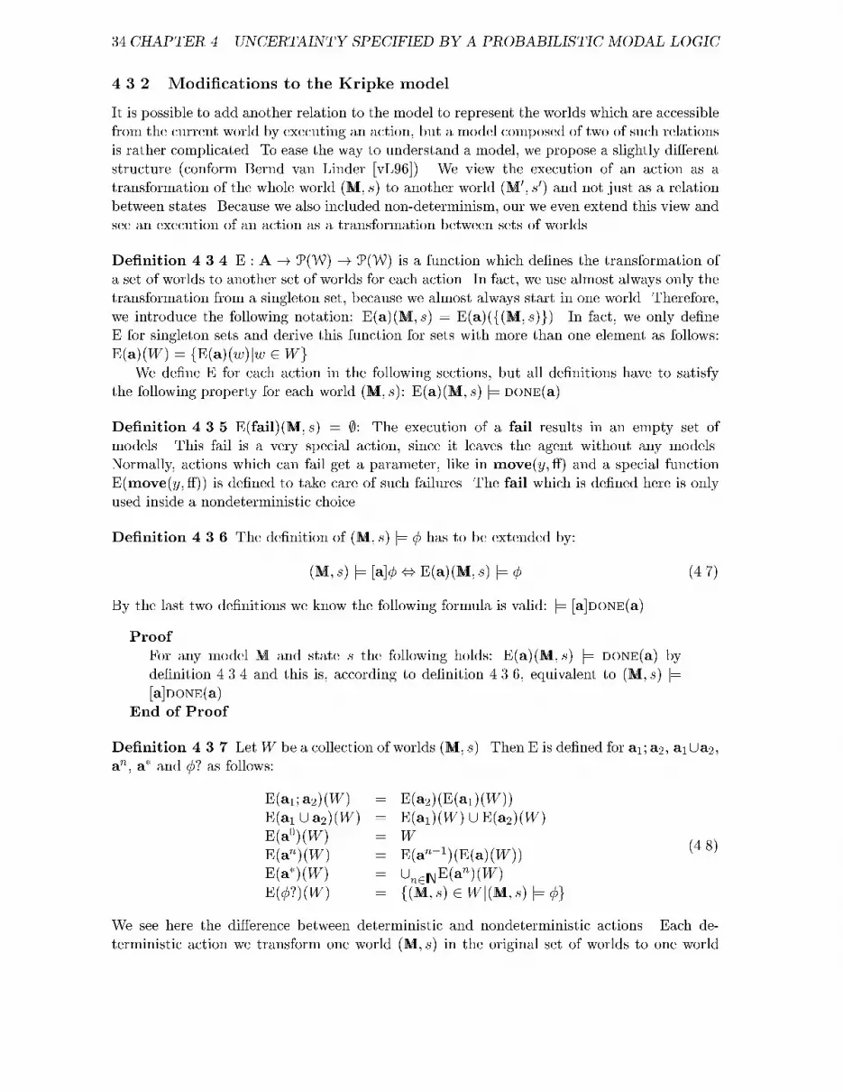
34CHAPTER 4. UNCERTAINTY SPECIFIED BY A PROBABILISTIC MODAL LOGIC4.3.2 Modi�cations to the Kripke modelIt is possible to add another relation to the model to represent the worlds which are accessiblefrom the current world by executing an action, but a model composed of two of such relationsis rather complicated. To ease the way to understand a model, we propose a slightly di�erentstructure (conform Bernd van Linder [vL96]). We view the execution of an action as atransformation of the whole world (MM; s) to another world (MM0; s0) and not just as a relationbetween states. Because we also included non-determinism, our we even extend this view andsee an execution of an action as a transformation between sets of worlds.De�nition 4.3.4 E : A! P(W) ! P(W) is a function which de�nes the transformation ofa set of worlds to another set of worlds for each action. In fact, we use almost always only thetransformation from a singleton set, because we almost always start in one world. Therefore,we introduce the following notation: E(a)(MM; s) = E(a)(f(MM; s)g). In fact, we only de�neE for singleton sets and derive this function for sets with more than one element as follows:E(a)(W ) = fE(a)(w)jw 2Wg.We de�ne E for each action in the following sections, but all de�nitions have to satisfythe following property for each world (MM; s): E(a)(MM; s) j= done(a).De�nition 4.3.5 E(fail)(MM; s) = ;: The execution of a fail results in an empty set ofmodels. This fail is a very special action, since it leaves the agent without any models.Normally, actions which can fail get a parameter, like in move(y;�) and a special functionE(move(y;�)) is de�ned to take care of such failures. The fail which is de�ned here is onlyused inside a nondeterministic choice.De�nition 4.3.6 The de�nition of (MM; s) j= � has to be extended by:(MM; s) j= [a]�, E(a)(MM; s) j= � (4.7)By the last two de�nitions we know the following formula is valid: j= [a]done(a).ProofFor any model MM and state s the following holds: E(a)(MM; s) j= done(a) byde�nition 4.3.4 and this is, according to de�nition 4.3.6, equivalent to (MM; s) j=[a]done(a).End of ProofDe�nition 4.3.7 LetW be a collection of worlds (MM; s). Then E is de�ned for a1;a2, a1[a2,an, a� and �? as follows:E(a1;a2)(W ) = E(a2)(E(a1)(W ))E(a1 [ a2)(W ) = E(a1)(W ) [ E(a2)(W )E(a0)(W ) = WE(an)(W ) = E(an�1)(E(a)(W ))E(a�)(W ) = [n2INE(an)(W )E(�?)(W ) = f(MM; s) 2W j(MM; s) j= �g (4.8)We see here the di�erence between deterministic and nondeterministic actions. Each de-terministic action we transform one world (MM; s) in the original set of worlds to one world

4.3. ADDING ACTIONS: DYNAMIC LOGIC 35T1T2position(0)obstacle(2)position(0)obstacle(3)0.80.2s T3T4position(0)obstacle(2)position(0)obstacle(3)observe(3)

0.80.2Figure 4.5: This model models B(position(0))! [observe(3)]pr(obstacle(3)) > 0:5.(MM0; s0) in the resulting set of worlds. However, a nondeterministic action creates more thanone world for each world in the original set. Since we start with one world, a sequence ofdeterministic actions results in one world.A nondeterministic action is in general a union of actions. If all but one of these actionsfail, the nondeterministic action is a sort of deterministic action after all (see de�nition 4.3.5).Example 4.3.8 The following propositions follow from the de�nitions above.1. [a1;a2]�$ [a1][a2]�2. [a1 [ a2]�$ [a1]� ^ [a2]�3. [�?]�$ (�! �)4. [a�]�$ � ^ [a][a�]�5. � ^ [a�](�! [a]�)! [a�]�Together these form the so-called Segerberg Axioms for dynamic logic, whose completenesswas proved by various authors including Rohit Parikh and Dexter Kozen [KP81].In the next section, we distinguish two types of actions. For now, we give an example for eachof these two types: observe and move. observe is a nondeterministic choice among severalobserve(c) actions, with c as the distance to the nearest obstacle. move(y) is a collectionof actions: one for each non-zero integer y. For example, if move(2) is executed, the agentmoves 2 cells to the front.Example 4.3.9 Consider the following examples:1. (MM; s) j= B(position(0)) ! [observe(3)]pr(obstacle(3)) > 0:5: If the agent believes itis at position 0 then after execution of the action observe(3) the agent believes thatthe probability of an obstacle being at position 3 is greater than 0:5. A model whichvalidates this formula is shown in �gure 4.5.2. (MM; s) j= pr(position(1)) = 0:9 ! [move(2)]pr(position(3)) = 0:9: In �gure 4.6 amodel is shown in which the following holds: If the agent believes the probability of itbeing at position 1 is 0:9 then after the execution ofmove(2), it believes the probabilityof it being at position 3 is also 0:9. In this case the agent believes it moved exactly 2.

36CHAPTER 4. UNCERTAINTY SPECIFIED BY A PROBABILISTIC MODAL LOGICs T3T4T1T2position(0)position(1)move(2)

position(3)position(2)0.90.10.10.9

Figure 4.6: This model models pr(position(1)) = 0:9! [move(2)]pr(position(3)) = 0:9.s T1 T2 T3T4observe(3)1 0.250.75 obstacle(2)Figure 4.7: This model models pr([observe(3)]pr(obstacle(2)) = 0:25) = 1.3. (MM; s) j= pr([observe(3)]pr(obstacle(2)) = 0:25) = 1: the agent believes with probabil-ity 1 that, after the execution of observe(3), it believes that the probability that thereis an obstacle at 2 is 14 , see �gure 4.7.4.4 Application: Simplebot in a linear worldIn this section we introduce a very simple robot in a very simple world. This situation isused to illustrate our theory. We distinguish two types of actions: pure informational actions,which do not change anything in the real world and actions which are really performed bythe agent. One action of each type is introduced: observe and move. Both these actionsare in practice imperfect: the informational actions don't always give the correct informationand the move action will often not move exactly the speci�ed distance. In this section weassume always �rst the actions to be perfect and thereafter give the guidelines how to handleuncertainty or imperfection.4.4.1 An exampleAssume we have a robot, called Simplebot with the following speci�cations:� Simplebot has several beliefs about its own position and the position of obstacles.� Simplebot has one sonar sensor which is always pointed towards the front.� For now Simplebot explores a world called Linearworld with the following properties:{ Linearworld is linear, therefore Simplebot can only move in one direction and isunable to turn.

4.4. APPLICATION: SIMPLEBOT IN A LINEAR WORLD 370 1 2 3 4Figure 4.8: Simplebot in Linearworld: Our simple robot with just one sensor and no turncapability in a linear world.{ To be able to talk about positions in the Linearworld in a convenient way, werepresent this world as a grid. We number the cells of this grid. To minimize thee�ect of rounding errors, we could take a very �ne grid.{ This particular Linearworld has one obstacle at position 2 and Simplebot itself isat position 0. The length of this Linearworld is �nite: grid numbers range from 0to 4. Figure 4.8 shows this world.� Simplebot is able to perform the following actions:{ observe observes a distance to the nearest obstacle in front of Simplebot. Thisaction is a nondeterministic choice among a set of observe(c) actions. observe(c)is the action which observes that the distance to the nearest obstacle is c or failsotherwise. Whether such an action fails is detected by the sonar. In this �rstexample we assume this observation is perfect. If there isn't any obstacle, theobservation with c equal to the distance to the end of the world is the only onethat doesn't fail.{ For each positive integer y Simplebot can perform move(y): move y to the front(or if y < 0, �y to the back).The value c in an observe(c) action and the parameter y of a move(y) action are thenumber of grid cells.Before the execution of an observe(c) action, the agent doesn't know what the result cwill be. Therefore we de�ne an observe action which is the nondeterministic choice amongall the possible values.De�nition 4.4.1 In general observe(c) is an informational action, which only observes thatthe distance to the nearest obstacle in the direction of the sensor is c grid cells. This actionhas no other e�ects. Suppose d is the distance to the end of the grid. We de�ne C as the setof all positive integer values between 1 and d: C = f1; 2; : : : ; dg.observe = [c2Cobserve(c), but in this example: observe = [c2f1;2;3;4gobserve(c).In a particular situation all but one of observe(c) actions will fail. Therefore, afterwards onecould say that the observe was equivalent to the observe(c) that didn't fail.De�nition 4.4.2 In general: move(y) is a performing action. After the execution of asucceeded move(y) the agent has moved y to the front or if y < 0, �y to the back. Insection 4.4.3 we discuss this action further.

38CHAPTER 4. UNCERTAINTY SPECIFIED BY A PROBABILISTIC MODAL LOGIC4.4.2 Incorporating the observe action in our languageAssume the robot believes position(0) and does a (correct) sensing action: observe(2). Asensor action will never add new states to our model. The only result of such an action is theassignment of other probabilities to some (groups of) states. In this example all states withan obstacle(1) get probability 0, just as all states without obstacle(2). The remaining statesget a new probability, so that the sum of all probabilities is still 1. The goal of this section isto de�ne the function E(observe(y)) which does exactly that.We de�ne the proposition nearest obstacle(x) for each state with propositions position(z)and obstacle(x) and x > 0. This proposition states that all cells of the grid between the currentposition of Simplebot and the nearest obstacle at position x+ z do not have an obstacle:De�nition 4.4.3position(z)! nearest obstacle(x)$ x�1̂i=1 :obstacle(z + i) ^ obstacle(z + x)! (4.9)In the Linearworld example only the obstacles in the direction of the sensor are considered,therefore x > 0.To be able to talk about the model before and after the execution of the action in aconvenient way, we use the following notation: the world before the execution is (MM; s) =((S; �;R;Pr); s) and the world after is (MM0; s0) = ((S0; �0;R0;Pr0); s0). Thus in every proof thefollowing holds: (MM0; s0) = E(observe(y))(MM; s).We would like to calculate the new probability of a state after executing an observe(y)action. Probability theory helps in de�ning such a new probability for a formula, like forexample nearest obstacle(�x). This probability can be written as a conditional probability:Pfnearest obstacle(�x)jobserved(y)g.Bayes' rule tells us how to calculate such an a posteriori probability. Suppose we havea partitioning of the set of possible result states: B = fB1; : : : ; Bng and for each 1 � i; j �n; i 6= j : Bi \ Bj = ; and suppose we would like to know the probability for each Bj ,while we already know that A. This probability, called the probability of Bj conditionedby A (PfBj jAg), is equal to the normalized probability of A conditioned by Bj times theprobability of Bj . PfBj jAg = PfAjBjg � PfBjgPi PfAjBig � PfBig (4.10)This rule is based on the de�nition of conditional probability: PfBj jAg = PfBj and AgPfAg (andtherefore also: PfAjBjg = PfBj and AgPfBjg ) and the theorem of of total probability: PfAg =Pni=1 PfAjBig � PfBig. The proof of this theorem, sometimes called the rule of elimination,can be found in any standard work on probability and statistics [Tri82]. The proof of Bayes'rule is rather straightforward: PfBj jAg = PfBj and AgPfAg= PfAjBjg�PfBjgPfAg= PfAjBjg�PfBjgPiPfAjBig�PfBig (4.11)We illustrate this rule by two examples.

4.4. APPLICATION: SIMPLEBOT IN A LINEAR WORLD 39Example 4.4.4 For example, suppose we have nine mice. Three white (B1), three grey (B2)and three black (B3) ones. One of the white ones misses an ear, two of the grey ones miss anear and all black ones miss an ear, because they like to nibble at each other. We'd like to knowthe probability that we have a white mouse (B1) conditioned that we know the mouse missesan ear (A). This is equal to the probability that a white mouse misses an ear (PfAjB1g = 13 )times the probability that we have a white mouse (13 ) divided by the sum of these productsfor all colors mice. For black this product is 33 � 13 and for grey 23 � 13 , so the sum is 23 . Thereforethe probability that we have taken a white mouse is 1923 = 16 .Example 4.4.5 Suppose we throw an ordinary dice. The probability that the result r is a 6provided that we know the result is an even number can be calculated using this rule:Pfr = 6jeveng = Pfevenjr = 6g � Pfr = 6gP6i=1 Pfevenjr = ig � Pfr = ig = 1 � 16Pi=1;3;5 0 � 16 +Pi=2;4;6 1 � 16 = 13 (4.12)We are now able to derive a rule speci�c for our model, but in fact it is the same as Bayes'rule. For this rule it doesn't matter whether observe is perfect, we come to this later. De�neX as the set of all grid numbers in front of the robot. For any �x 2 X:Lemma 4.4.6 Psfnearest obstacle(�x)jobserved(y)g == Psfobserved(y)jnearest obstacle(�x)g�Psfnearest obstacle(�x)gPx2X Psfobserved(y)jnearest obstacle(x)g�Psfnearest obstacle(x)g (4.13)The one step proof derives this lemma directly from Bayes' rule (equation (4.10)).Compare this formula with the de�nition of Bel(distance = t; s0) in section 3.2. It is notvery di�cult to see that both approaches have the same Bayesian basis.We want to de�ne the function Pr0 such that it satis�es this version of Bayes' rule. We thinkBayes' rule is a good way to model the change of probabilities. In the following de�nition thevariables with a quote are the new ones, which are derived from the old ones and observed(y)is the proposition that states that the last executed action was observe(y).De�nition 4.4.7 We de�ne E for observe:E(observe(y))((S; �;R;Pr); s) = ((S0; �0;R0;Pr0); s0) (4.14)with S0 = S, R0 = R and s0 = s. For each state t there exist precisely one �xt such that(MM; t) j= nearest obstacle(�x) (if not we take xt to be equal to the largest cell number inthe grid). The probability measure Pr0 between the states s0 and t0 after the execution ofobserve(y) is de�ned as follows:Pr0(s0; t0) = Psfobserved(y)jnearest obstacle( �xt)g � Pr(s; t)Px2X (Psfobserved(y)jnearest obstacle(x)g � Pr(s; [[nearest obstacle(x)]]s))(4.15)and the truth assignment de�ned as follows for each �0 2 S0:�0(�0)(p) = ( if p = done(observe(y)) and �0 = s0 then ttotherwise �(�)(p) (4.16)

40CHAPTER 4. UNCERTAINTY SPECIFIED BY A PROBABILISTIC MODAL LOGICThe term Psfobserved(y)jnearest obstacle( �xt)g de�nes the probability that a distance yis observed, when the distance to the nearest obstacle is assumed to be �xt. In fact, thisexpresses the error measure of the sensor and this should be de�ned seperately. We come tothis later (equations (4.20) and (4.24)). The denominator in the de�nition above looks ratherdi�cult, but it just normalizes all the fractions so they sum up till 1. The result of applyingthis de�nition is a redistribution of the probabilities: some of the probabilities are 0 becausethe nearest obstacle in that particular world ( �xt) is out of range concerning the observeddistance (y). In other words: Psfobserved(y)jnearest obstacle( �xt)g = 0. The probabilities ofall the other worlds rise because they should still sum up till 1.Example 4.4.8 We show how this de�nition can be used to calculate the new probabili-ties, Pr0. Suppose we have the probabilities as shown in �gure 4.3 and the agent does anobserve(2) action. Suppose furthermore Psfobserved(2)jnearest obstacle(2)g = 0:5 andPsfobserved(2)jnearest obstacle(3)g = 0:25. (Now, we are running ahead of what we havetold, because this implicitely means that we cope with a noisy sensor.) The new probabilitiesare calculated as follows:Pr0(s0; T 01) = Psfobserved(2)jnearest obstacle(2)g�Pr(s;T1)Px2f2;3g�Pr(s;T1)(Psfobserved(2)jnearest obstacle(x)g�Pr(s;[[nearest obstacle(x)]]s))= 0:5�0:50:5�0:8+0:25�0:2 = 0:250:45Pr0(s0; T 02) = Psfobserved(2)jnearest obstacle(2)g�Pr(s;T2)Px2f2;3g(Psfobserved(2)jnearest obstacle(x)g�Pr(s;[[nearest obstacle(x)]]s))= 0:150:45Pr0(s0; T 03) = Psfobserved(2)jnearest obstacle(3)g�Pr(s;T3)Px2f2;3g(Psfobserved(2)jnearest obstacle(x)g�Pr(s;[[nearest obstacle(x)]]s))= 0:050:45 (4.17)Theorem 4.4.9 De�nition 4.4.7 satis�es the instance of Bayes' rule from lemma 4.4.6. Inother words: Pr0(s0; [[nearest obstacle(�x)]]s0) == Psfobserved(y)jnearest obstacle(�x)g�Psfnearest obstacle(�x)gPx2X Psfobserved(y)jnearest obstacle(x)g�Psfnearest obstacle(x)g (4.18)ProofWe express Pr0(s0; [[nearest obstacle(�x)]]s0) in the sum over all states in the set ofstates T 0 = [[nearest obstacle(�x)]]s0 using de�nition 4.2.3. Here we �ll in de�ni-tion 4.4.7. Then we rewrite this fraction using de�nitions 4.2.3 again and equa-tion 4.5.Pr0(s0; [[nearest obstacle( �x)]]s0) ==Pt02T 0 Pr0(s0; t0) ==Pt02T 0 Psfobserved(y)jnearest obstacle(�x)g�Pr(s;t)Px2X(Psfobserved(y)jnearest obstacle(x)g�Pr(s;[[nearest obstacle(x)]]s)) == Psfobserved(y)jnearest obstacle(�x)g�(Pt02T 0 Pr(s;t))Px2X(Psfobserved(y)jnearest obstacle(x)g�Pr(s;[[nearest obstacle(x)]]s)) == Psfobserved(y)jnearest obstacle(�x)g�Pr(s;[[nearest obstacle(�x)]]sPx2X(Psfobserved(y)jnearest obstacle(x)g�Pr(s;[[nearest obstacle(x)]]s)) == Psfobserved(y)jnearest obstacle(�x)g�Psfnearest obstacle(�x)gPx2X(Psfobserved(y)jnearest obstacle(x)g�Psfnearest obstacle(x)g) (4.19)

4.4. APPLICATION: SIMPLEBOT IN A LINEAR WORLD 41End of ProofDirectly from theorem 4.4.9 and lemma 4.4.6, we get the following equation:Corollary 4.4.10 Pr0(s0; [[nearest obstacle(x)]]s0) = Psfnearest obstacle(x)jobserved(y)gThis is exactly how we wanted to have Pr0 de�ned.A perfect sensor actionTo be able to use de�nition 4.4.7 we have to de�ne the conditional probabilities for eachintegers x and y, Psfobserved(y)jnearest obstacle(x)g. As our observations are perfect wede�ne these probabilities as follows for any state s:Psfobserved(y)jnearest obstacle(x)g = ( if x� y = 0 then 1:0otherwise 0 (4.20)Example 4.4.11 Consider the following examples.1. Consider a Linearworld of size �ve. Simplebot is at position 0 and there is no obstacleat position 0. Take V as the set of all possible combinations of obstacles in the gridpositions 1, 2, 3 and 4. There are 16 groups of states reachable from the currentworld (MM; s); a group of states for each element of V . Take i as the number of perfectobserve(2) actions. In the table 4.1 we show the probabilities for each group of statesbefore (Pr(V )) and after (Pr(i)(V )) i observe(2) actions.The following formulae, derived from de�nition 4.4.7, have been used (with X =f1; 2; 3; 4g:Pr(1)(V ) = Psfobserved(2)jnearest obstacle(min(V ))g � Pr(V )Px2X(Psfobserved(2)jnearest obstacle(x)g � Pr(s; [[nearest obstacle(x)]]s))(4.21)Pr(2)(V ) = Ps0fobserved(2)jnearest obstacle(min(V ))g � Pr(1)(V )Px2X(Ps0fobserved(2)jnearest obstacle(x)g � Pr(s0; [[nearest obstacle(x)]]s0))(4.22)In this formula min(V ) symbolizes the smallest element of V and thus the position ofthe nearest obstacle.It does not suprise us that the only state-collections with a positive probability arethose which model nearest obstacle(2), because all the other counters are a product ofPsfobserved(2)jnearest obstacle(x)g for x 6= 2 and for a perfect sensor, this probabilityis 0. Neither does it suprise us that a second observe(2) action did not add anyinformation, since the �rst action was perfect and already gave all the information.From table 4.1 and equations (4.1) and (4.9), we are able to calculate �i and �(1)i fori = 1; 2; 3 or 4 in the following formula: (MM; s) j= pr(nearest obstacle(i)) = �i before(�i) and after (�(1)i ) the observe(2) action was completed. In table 4.2, we also addedPsfobserved(2)jnearest obstacle(i)g, so the values can be easily veri�ed.We calculated these values as follows:�(j)i = XV 2fV jV 2P(f1;2;3;4g)^min(V )=igPr(j)(V ) (4.23)

42CHAPTER 4. UNCERTAINTY SPECIFIED BY A PROBABILISTIC MODAL LOGICTable 4.1: The probabilities of a group of states V after 1 and after 2 times the execution ofa perfect observe(2) action. V Pr(V ) Pr(1)(V ) Pr(2)(V )116 0 01 116 0 02 116 14 142; 1 116 0 03 116 0 03; 1 116 0 03; 2 116 14 143; 2; 1 116 0 04 116 0 04; 1 116 0 04; 2 116 14 144; 2; 1 116 0 04; 3 116 0 04; 3; 1 116 0 04; 3; 2 116 14 144; 3; 2; 1 116 0 0Table 4.2: The probabilities of nearest obstacle(i) for i = 1; : : : ; 4 after 1 and 2 observe(2)actions, calculated using table 4.1.i Psfobserved(2)jnearest obstacle(i)g �i �(1)i �(2)i1 0 12 0 02 1 14 1 13 0 18 0 04 0 116 0 0

4.4. APPLICATION: SIMPLEBOT IN A LINEAR WORLD 4300.10.20.30.40.50.6

-2 -1 0 1 2Figure 4.9: The probability distribution of Psfobserved(y)jnearest obstacle(x)g2. From the example above, it is easy to see that the following formula is valid: (MM; s) j=pr(nearest obstacle(2)) = 14 ^ position(0) ! [observe(2)]pr(nearest obstacle(2)) = 1:if the agent believes the nearest obstacle to be two positions ahead with probability 14and the agent is at position 0, then, after execution of a perfect observe(2) action, theagent believes that this probability is 1.A noisy sensor actionSuppose the sensor of Simplebot is not perfect. We assume there exists a probability distri-bution which describes the error of the sonar. An example of such a distribution can be foundin �gure 4.9.For now we use the following discrete normal distribution to de�ne the conditional prob-ability Psfobserved(y)jnearest obstacle(x)g for any state s:Psfobserved(y)jnearest obstacle(x)g = approxnormal(x� y)approxnormal(i) = 8>>><>>>: if i = �1 then 0:25if i = 0 then 0:5if i = 1 then 0:25otherwise 0:0 (4.24)Consider a Linearworld of size �ve. Simplebot is at position 0 and there is no obstacle atposition 0. Take V as the set of all possible combinations of obstacles in the grid positions1, 2, 3 and 4. There are 16 states reachable from the current world (MM; s); a state for eachelement of V . In table 4.3 we show the probabilities for each state before (Pr(V )) and after(Pr(i)(V )) i observe(2) actions with noise. The same formulae as in the previous examplehave been used.From table 4.3 and equations (4.1) and (4.9), we are able to calculate �i and �0i fori = 1; 2; 3; 4 in the following formula: (MM; s) j= pr(nearest obstacle(i)) = �i before (�i) andafter (�0i) the observe(2) action was completed. In table 4.4, we also added the value ofPsfobserved(2)jnearest obstacle(i)g, so the calculations using de�nition 4.4.7 can be easilyveri�ed.We see that the probability that the nearest obstacle is at position 2, increases with thenumber of observe actions. This fact leaves us the opportunity to demand a certain certaintybefore executing an action.

44CHAPTER 4. UNCERTAINTY SPECIFIED BY A PROBABILISTIC MODAL LOGICTable 4.3: The probabilities of a group of states V after 1 and after 2 times the execution ofa noisy observe(2) action. V Pr(V ) Pr(1)(V ) Pr(2)(V )116 0 01 116 118 1262 116 218 4262; 1 116 118 1263 116 118 1263; 1 116 118 1263; 2 116 218 4263; 2; 1 116 118 1264 116 0 04; 1 116 118 1264; 2 116 218 4264; 2; 1 116 118 1264; 3 116 118 1264; 3; 1 116 118 1264; 3; 2 116 218 4264; 3; 2; 1 116 118 126Table 4.4: The probabilities of nearest obstacle(i) for i = 1; : : : ; 4 after 1 and 2 observe(2)actions, calculated using table 4.2.i Psfobserved(2)jnearest obstacle(i)g �i �(1)i �(2)i �(3)i1 14 12 49 413 4212 12 14 49 813 16213 14 18 19 113 1214 0 116 0 0 0

4.4. APPLICATION: SIMPLEBOT IN A LINEAR WORLD 45

00.20.40.60.81

0 0.5 1 1.5 2 2.5 3 3.5 4

� 33 3 3 3

�0 ++ +

+ +

�00 22 2

2 2�000 �

��

� �Figure 4.10: The probability of the nearest obstacle being at positions 1, 2, 3 and 4 before anyobservations (�), after one observation (�(1)), two observations (�(2)) and three observations(�(3)). It is easy to see that the probability of the nearest obstacle existing at position 2increases.4.4.3 Incorporating a move action in our languageIn this section we de�ne E(move(y)). To simplify matters, we �rst de�ne a move(1) action.The perfect execution of this action results in a world in which the robot has moved one cellin the grid to the front.When a robot executes a move command, the result could be one out of the followingsituations.� The robot has moved one cell to the front. We de�ne this to be a move(1; tt) action.� The robot stopped during the movement, because an obstacle blocked its way. Wede�ne this to be a move(1;�) action.Therefore we de�ne the move(1) to be the nondeterministic choice among a move(1; tt) anda move(1;�).De�nition 4.4.12 move(1) :=move(1; tt) [move(1;�).We describe now how the model changes by the di�erent types of move actions.Perfect moveAmove(1; tt) retains all the states except the ones in which there should have been a collision(x � 1 in nearest obstacle(x)). These states get a probability of 0. The probabilities forthe other states are redistributed. The propositions for a state � changes as follows: eachposition(z�) becomes position(z� + 1).

46CHAPTER 4. UNCERTAINTY SPECIFIED BY A PROBABILISTIC MODAL LOGICDe�nition 4.4.13 We de�ne E as follows for a perfect move:E(move(1; tt))((S; �;R;Pr); s) = ((S0; �0;R0;Pr0); s0) withS0 = S � fsj(MM; s) j= nearest obstacle(x) for x = 0; 1g, s0 = s and �0, R0 and Pr0 de�ned inthe following way.For any state � in our model with this application there exists precisely one z� 2 ZZ suchthat (MM; �) j= position(z�). Since no other atomic propositions are changed by move, wede�ne for each �0 2 S0:�0(�0)(p) = 8>>><>>>: if p = done(move(1; tt)) and �0 = s0 then ttif p = position(z�) then �if p = position(z� + 1) then ttotherwise �(�)(p)The new accessibility relation is almost the same as the old one: R0(s0; t0) , (R(s; t) ands0; t0 2 S0). When we de�ne T to be the set of all old states t that are successors of s bythe new relation R0 (T := ftjR0(s; t)g), Pr0 can be de�ned as: Pr0(s0; t0) = Pr(s;t)Pr(s;T ) . Thedenominator makes sure the new probabilities sum up till one.A move(1;�) changes the model in the opposite way: all states in which there shouldhave been a collision remain and the probabilities are redistributed for these states. Since therobot has failed to move, no propositions should be adjusted.De�nition 4.4.14 We de�ne E as follows for a move without noise:E(move(1;�))((S; �;R;Pr); s) = ((S0; �0;R0;Pr0); s0) withS0 = S � fsj(MM; s) j= nearest obstacle(x) for x = 2; : : :g, �0 = �, s0 = s and R0 and Pr0de�ned as follows.The new accessibility relation is almost the same as the old one: R0(s0; t0) , R(s; t) ands0; t0 2 S0. When we de�ne T := ftjR0(s; t)g, it is rather easy to de�ne Pr0: Pr0(s; t) = Pr(s;t)Pr(s;T ) .Again, the denominator is just added to normalize the probabilities.Suppose the agent executes y timesmove(1; tt). Probably this will occur often. Thereforewe name this move(y; tt).De�nition 4.4.15 move(y; tt),movey(1; tt)In the same way we de�ne move(y;�), meaning that the agent actually moved y� 1, butcould not move one further.De�nition 4.4.16 move(y;�),move(y � 1; tt);move(1;�)Finally, we are able to de�ne move(y) as a nondeterministic choice among move(y; tt)and a couple of move(y;�):De�nition 4.4.17 move(y),move(y; tt) [ [i=1;:::;ymove(i;�)Theorem 4.4.18 For any y 2 IN, y 6= 0 and move without noise the following holds:E(move(y; tt))((S; �;R;Pr); s) = ((S0; �0;R0;Pr0); s0) whereS0 = S � fsj(MM; s) j= nearest obstacle(x) for x � yg

4.4. APPLICATION: SIMPLEBOT IN A LINEAR WORLD 47, s0 = s and �0, R0 and Pr0 as de�ned in the following way.For any state � in our model there exists precisely one z� 2 ZZ such that (MM; �) j=position(z�). No other atomic propositions are changed by move, therefore, for each �0 2 S0,�0 shows as follows:�0(�0)(p) = 8>>><>>>: if p = done(move(y; tt)) and �0 = s0 then ttif p = position(z�) then �if p = position(z� + y) then ttotherwise �(�)(p)The new accessibility relation is almost the same as the old one: R0(s0; t0), R(s; t) and s0; t0 2S0. When we de�ne T := ftjR0(s; t)g, Pr0 is equal to: Pr0(s0; t0) = Pr(s;t)Pr(s;T ) . The denominatormakes sure the new probabilities sum up till one.ProofThis theorem is proven with induction to y. The basic case is when y = 1. Thetheorem is then exactly the same as de�nition 4.4.13 and therefore trivially valid.The induction hypothesis sounds as follows: suppose the theorem is valid fory = n� 1, then the theorem is also valid for y = n.Suppose the theorem is valid for y = n � 1. We split the execution ofmove(n; tt): move(n � 1; tt);move(1; tt). We notate (MM00; s00) as the interme-diate model E(move(n � 1; tt))(MM; s) and (MM0; s0) = ((S0; �0;R0;Pr0); s0) as theresulting model E(move(1; tt))(MM00; s00).S00 = S � fsj(MM; s) j= nearest obstacle(x) for x � n � 1g and S0 = S00 �fs00j(MM00; s00) j= nearest obstacle(x) for x � 1g by de�nition 4.4.13. We knowthat (MM00; s00) j= position(zs+n�1)^�(n�1)�i��1:obstacle(zs+n�1+ i) (by thede�nition of S00 and nearest obstacle) and (MM; s) j= position(zs), so (MM00; s00) j=position(zs+n�1)^nearest obstacle(1)^�(n�1)�i��1:obstacle(zs+n�1+ i) isequivalent to (MM; s) j= position(zs)^nearest obstacle(n�1+1) by de�nition 4.4.3.Therefore, S0 = S � fsj(MM; s) j= nearest obstacle(x) for x � n� 1g�fs00j(MM00; s00) j= nearest obstacle(1)g == S � fsj(MM; s) j= nearest obstacle(x) for x � n� 1g�fsj(MM; s) j= nearest obstacle(n� 1 + 1)g == S � fsj(MM; s) j= nearest obstacle(x) for x � ngand s0 = s00 = s. About �00 and �0 we know:�00(s00)(p) = 8><>: if p = position(zs) then �if p = position(zs + n� 1) then ttotherwise �(s)(p)and �0(s0)(p) = 8><>: if p = position(zs00) then �if p = position(zs00 + 1) then ttotherwise �00(s00)(p)

48CHAPTER 4. UNCERTAINTY SPECIFIED BY A PROBABILISTIC MODAL LOGICzs00 = zs + n� 1 thus the above two equations can be combined to:�0(s0)(p) = 8>>>>><>>>>>: if p = position(zs00) then �if p = position(zs + n� 1 + 1) then ttelse if p = position(zs) then �else if p = position(zs + n� 1) then ttotherwise �(s)(p)The fourth choice is overwritten by the �rst and the �rst is obsolete, because�(s)(position(z)) is only true for z = zs. Therefore, this is equivalent to�0(s0)(p) = 8><>: if p = position(zs + n) then ttif p = position(zs) then �otherwise �(s)(p)Since R0(s0; t0), R00(s00; t00) and s0; t0 2 S0 and R00(s00; t00), R(s; t) and s00; t00 2S00, we know that R0(s0; t0) , R(s; t) and s00; t00 2 S00 and s0; t0 2 S0 and thusR0(s0; t0), R(s; t) and s0; t0 2 S0.Finally, we derive Pr0(s0; t0) as follows: Pr0(s0; t0) is equal to the normalizedvalues of Pr00(s00; t00) and Pr00(s00; t00) is equal to the normalized value of Pr(s; t),so Pr0(s0; t0) is equal to the normalized values of Pr(s; t) (with T = ftjR0(s; t)g:Pr0(s0; t0) = Pr(s;t)Pr(s;T ) . Now, the induction hypothesis is proven and thereby thetheorem except for done(move(y; tt)). This last one can be done by addinga de�nition like: (MM; s00) j= done(move(y � 1); tt) and E(move(1; tt))(MM; s00) j=done(move(1; tt)) so E(move(1; tt))(MM; s00) j= done(move(y�1; tt);move(1; tt))which is equivalent to (MM; s0) j= done(move(y; tt)).End of ProofIf move(y; tt) is noisy, move(y; tt) is not equal anymore to movey(1; tt), because manyshort moves probably create a larger error than one large move due to extra slipping whilestarting and braking. Therefore such a theorem does not hold is move(y; tt) is noisy.Example 4.4.19 We prove three valid formulae to illustrate the possibilities of this language.1. j= position(2)! [move(5; tt)]position(7): If the agent is at position 2, it is at position7 after the execution of move(5; tt).ProofSuppose we have a world (MM; s) such that (MM; s) j= position(2).We know that zs = 2 and y = 5. Now, theorem 4.4.18 tells us the following:�0(s0)(position(7)) = �0(s0)position(2 + 5) = �0(s0)(position(zs + y) = tt.Thus E(move(5; tt))(MM; s) j= position(7). Using de�nition 4.3.6 we knowthat (MM; s) j= [move(5; tt)]position(7).Because we supposed for a random world (MM; s) that (MM; s) j= position(2),j= position(2)! [move(5; tt)]position(7) holds.End of Proof

4.4. APPLICATION: SIMPLEBOT IN A LINEAR WORLD 492. j= pr(position(2)) = 0:9 ^B(nearest obstacle(3))! [move(2)](pr(position(2)) = 0:9 _pr(position(3)) = 0:9 _ pr(position(4)) = 0:9): If the agent believes with probability0:9 that it is at position 2 and it believes the nearest obstacle to be 3 cells ahead (atposition 5), then after the execution of move(2) the agent believes it is at position 2with probability 0:9 or at position 3 with probability 0:9 or at position 4 with probability0:9. See also example 4.4.20 and �gure 4.11 for a slightly di�erent example.ProofSuppose we have a world (MM; s) such that (MM; s) j= pr(position(2)) � 0:9 ^B(nearest obstacle(3)).With T = ftjR(s; t) and (MM; t) j= position(2) ^ nearest obstacle(3)g weknow thatPt2T Pr(s; t) = 0:9. By de�nition 4.4.17 we know thatmove(2),move(2; tt) [move(2;�) [move(1;�). Because we deal here with a nonde-terministic action, we get a set of worlds as result. In fact we get a set with amodel for each of the three deterministic actions of which the nondeterministicmove(2) consists.(MM01; s01) = E(move(2; tt))(MM; s). De�ne T = ftjR(s; t)g and de�ne T 0 =ft0jR0(s0; t0)g. S0 = S�fsj(MM; s) j= nearest obstacle(x) for x = 0; 1g and T \fsj(MM; s) j= nearest obstacle(x) for x = 0; 1g = ; because for all t such thatR(s; t): (MM; t) j= nearest obstacle(3). So, using theorem 4.4.18 we concludethat T 0 = T . And therefore Pt02ft0jR0(s0;t0) and (MM0;t0)j=position(4)g Pr0(s0; t0) =Pt2ftjR(s;t) and (MM;t)j=position(2)g Pr(s; t) = 0:9, so (MM01; s01) j= pr(position(4)) =0:9.(MM02; s02) = E(move(1;�))(MM; s). Just as above, T 0 = T and now � isn'tchanged (see de�nition 4.4.14), so (MM02; s02) j= pr(position(2)) = 0:9.(MM03; s03) = E(move(2;�))(MM; s). Sincemove(2;�),move(1; tt);move(1;�),the result is a mix of the two situations described above. In an analog waywe can derive: (MM03; s03) j= pr(position(3)) = 0:9.Using de�nitions 4.2.3 and 4.3.4, we see that f(MM01; s01); (MM02; s02); (MM03; s03)g j=pr(position(2)) = 0:9 _ pr(position(3)) = 0:9 _ pr(position(4)) = 0:9, sowe conclude: (MM; s) j= [move(2)](pr(position(2)) = 0:9 _ pr(position(3)) =0:9 _ pr(position(4)) = 0:9).End of Proof3. j= B(position(2)) ^ B(nearest obstacle(6))) ^ B(nearest obstacle(1))): If the agent believes it is atposition 2 and the nearest obstacle is 6 cells ahead, then after a failed move of 4, itbelieves it is at position 5 and the nearest obstacle is at position 1. (The move failedbecause of the unknown obstacle at position 6.)ProofSuppose that (MM; s) j= B(position(2)) ^ B(nearest obstacle(6)) for a world(MM; s).We use theorem 4.4.18 again. We know that for all t such that R(s; t):zt = 2 by de�nition 4.2.4. We split move(4;�) according to de�nition 4.4.16:move(3; tt);move(1;�). We write (MM00; s00) = E(move(3; tt))(MM; s) and(MM0; s0) = E(move(1;�))(MM00; s00). By theorem 4.4.18 it holds for y = 3, thatfor all t such that R(s; t): �00(t00)(position(5) = �00(t00)(position(zs + y) = tt.

50CHAPTER 4. UNCERTAINTY SPECIFIED BY A PROBABILISTIC MODAL LOGICT1T20:10:90:90:10:90:1

0:90:1move(1;�)move(2;�)move(2; tt)

T3T4 T5T6T7T8t3 t2t1s

position(4) position(3)position(2)position(2)

Figure 4.11: This model validates pr(position(2)) = 0:9 ! [move(2)](pr(position(2)) =0:9 _ pr(position(3)) = 0:9 _ pr(position(4)) = 0:9).T1T20:10:9s position(2) T3position(2)position(3)position(4)move(1;�)move(2; tt)move(2;�) T4T5Figure 4.12: This model validates pr(position(2)) = 0:9 ! pr([move(2)](position(2) _position(3) _ position(4))) = 0:9.De�nition 4.4.14 tells us �0 = �00 and therefore for all t0 such that R(s0; t0):(MM0; t0) j= position(5) and thus (MM0; s0) j= B(position(5).De�nition 4.4.14 tells us also: S0 = S�fsj(MM; s) j= nearest obstacle(x) for x =2; : : :g, so for all states t: (MM0; s0) j= nearest obstacle(1) and thus (MM0; s0) j=B(nearest obstacle(1)).By simple manipulation of de�nition 4.2.3 we derive: (MM0; s0) j= B(position(5)^B(nearest obstacle(1)) and since we supposed to have a world (MM; s) such that(MM; s) j= B(position(2))^B(nearest obstacle(6)), we now know j= B(position(2))^B(nearest obstacle(6))! [move(4;�)]B(position(5))^B(nearest obstacle(1))is valid in all worlds.End of ProofIn fact, for any y the following holds: j= [move(y;�)]B(nearest obstacle(1).Example 4.4.20 The following two formulae are almost alike, but their models are quitedi�erent. The �rst formula is the most usual one. In its model the execution of a move(2)can be seen as a transformation between models.

4.4. APPLICATION: SIMPLEBOT IN A LINEAR WORLD 511. (MM; s) j= pr(position(2)) = 0:9) = 0:9 _ pr(position(3)) = 0:9 _ pr(position(4)) = 0:9): Ifthe agent believes with probability 0:9 that it is at position 2, then after the executionof move(2) the agent believes it is at position 2 with probability 0:9 or at position 3with probability 0:9 or at position 4 with probability 0:9. This model can be seen in�gure 4.11.2. (MM; s) j= pr(position(2)) = 0:9! pr([move(2)](position(2)_position(3)_position(4))) =0:9: If the agent believes with probability 0:9 that it is at position 2, then it believeswith probability 0:9 that after the execution ofmove(2) it is at position 2 or at position3 or at position 4. This model can be seen in �gure 4.12.Adding noiseIt is possible the robot does a move(y; tt) but in the real world just moves somewhat moreor less. This means extra states have to be introduced for each state with position(z). Inthe new model there should not just be one state with everything the same except for aposition(z + y), but also states with position(z + y � 1) and position(z + y + 1) and so on.We name these states, based on s, si and they have all the same propositions as s, but forposition which is position(z + y + i) with i 2 ZZ. New states which have an obstacle at thesame position as the agent believes himself to be are removed.De�nition 4.4.21 We de�ne a formula which states how much the agent has moved in realityduring the execution of a move(y; tt).position(z)! (real move(y + i)$ [move(y; tt)]position(z + y + i))The formula real move(y) is only used in context of Psfreal move(y + i)jmoved(y; tt)g,which is the probability that the agent has really moved y+ i where it should have moved y.This conditional probability is a function and a property of the robot. If this function is de�nedto be one if i = 0 and zero otherwise, move is perfect. If this function is de�ned in any otherway, we call the move noisy. In our example, we de�ne Psfreal move(y + i)jmoved(y; tt)gto be equal to approxnormal(i), which is de�ned by equation (4.24). In practice often the noiseand thus this function is dependent on the distance travelled.Because noise is introduced, a move(y; tt) is not exactly the same anymore as a sequenceof y times move(1; tt). This depends on the de�nition of Psfreal move(y+ i)jmoved(y; tt)g.Therefore we now de�ne E for each y.De�nition 4.4.22 We de�ne E as follows for any positive integer y:E(move(y; tt))((S; �;R;Pr); s) = ((S0; �0;R0;Pr0); s0) with S0 = fsijs 2 S and i 2 ZZg, s0 = sand �0, R0 and Pr0 as de�ned as follows:For any state s in our model there exists one zs 2 ZZ such that (MM; s) j= position(zs). �0is de�ned for each si 2 S0 as follows:�0(si)(p) = 8>>><>>>: if p = done(move(y; tt)) and si = s0 then ttif p = position(zs + y + i) then ttif p = position(x) and x 6= zs + y + i then �otherwise �(s)(p)

52CHAPTER 4. UNCERTAINTY SPECIFIED BY A PROBABILISTIC MODAL LOGICTable 4.5: The probabilities of groups of states de�ned by V = fv1; v2g after the execution of1 and 2 noisy move(1) actions which resulted in moved distance in the real world of v1 andv2. V Pr(1)(V ) Pr(2)(V )0; 0 14 1160; 1 14 180; 2 14 1161; 0 12 181; 1 12 141; 2 12 182; 0 14 1162; 1 14 182; 2 14 116The new accessibility relation is almost the same as the old one: R0(s0; ti), R(s; t) and s0; ti 2S0. When we de�ne T := ftjR(s; t) and s; t 2 Sg we de�ne Pr0 as follows:Pr0(s; ti) = Psfreal move(y + i)jmoved(y; tt)g � Pr(s; t)Pt2T Pi2ZZ Psfreal move(y + i)jmoved(y; tt)g � Pr(s; t)In fact, this is almost the same as de�nition 4.4.13, but now the new probability for statet0 has to be divided among the ti's. Because we suppose the noise is random, the valuePsfreal move(y + i)jmoved(y; tt)g is independent of the state t. Therefore we can just mul-tiply this by the probability of state t. The denominator, again, is just added to ensurenormalization.A move(y;�) changes the model as follows: �rst all the changes (like above) for a noisymove(y � 1; tt) are done. Thereafter the model is changed in the same way as while using aperfect move(1;�) command. Indeed, we assume that the robot is perfectly able to establishwhether the move command succeeded or not. So all states without a nearest obstacle(1)are removed.Example 4.4.23 Consider a Linearworld of size �ve. Simplebot is at position 0 and thereis no obstacle at all. We execute two consecutive noisy move(1) actions. Take V as the setof all possible combinations of two consecutive real moved distances: 0, 1, or 2. Two suchvalues de�ne a group of states. There are 3 � 3 groups of states reachable from the currentworld (MM; s); a group for each element of V . In table 4.5 we show the probabilities for eachgroup after (Pr(i)(V )) i move(1) actions.When we summarize these results we get the probabilities for position after 1 and 2move(1) actions as shown in table 4.6.As we can see, the probabilities become lower after more move actions. This is exactlythe reverse of what happened after several observe actions. However, this is not unexpected:a move actions does introduce uncertainty and an observe action tries to remove it.We calculate the probability of a proposition by summing over all the states in the modelwhich validates this proposition. Now, we introduce a way to de�ne and visualize probabilities

4.4. APPLICATION: SIMPLEBOT IN A LINEAR WORLD 53Table 4.6: The probabilities of position(i) for i = 0; : : : ; 4 after 0, 1 and 2 move(1)'s. Theseresults are calculated using table 4.5.i pr(position(i)) [move(1)]pr(position(i)) [move(1)][move(1)]pr(position(i))0 1 14 1161 0 12 142 0 14 383 0 0 144 0 0 116for certain propositions in a more natural and compact way. The probabilities for, for example,obstacle can be drawn in a probability map. In this map the probability pr(obstacle(x)) isassigned to the cell x for each x.De�nition 4.4.24 A proposition scheme is a function which accepts certain parameters andreturns a proposition. A mappable proposition scheme, in short mps, is a proposition schemewhich accepts only coordinates to create a proposition.mps = ZZn ! PDe�nition 4.4.25 We de�ne a probability map for a world (MM; s) to be a function for acertain mappable proposition scheme p : mps from an element in the space to a probability. nis the dimension of the space. probmaps = mps! ZZn ! [0; 1]We also de�ne a special version of a probability map. This version is called a probabilitydistribution. Some mappable proposition schemes, like position, are only valid for one positionin s. Thus the sum of the probabilities of all the states in which this proposition holds forany location should be exactly 1.De�nition 4.4.26 We de�ne a probability distribution, probdiss, as a special version of aprobability map (de�nition 4.4.25), such that for a mps p:Xz2ZZn probdiss(p)(z) = 1The following should hold for the associated model (MM; s):X(t;x1;:::;xn)2f(t;x1;:::;xn)jR(s;t)^(MM;t)j=p(x1;:::;xn)^x2ZZngPr(s; t) = 1 (4.25)Both a probability map for obstacle and a probability distribution for position can beseen in the left side of �gure 4.14.We also introduce a new way to visualize a collection of states. In �gure 4.13 the collectionof all states t is shown in which the following propositions hold: position(0), for all x 6= 0::position(x), obstacle(2), for all x 6= 2: :obstacle(2).

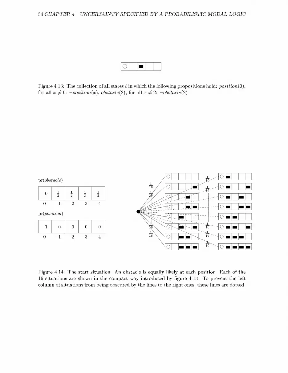
54CHAPTER 4. UNCERTAINTY SPECIFIED BY A PROBABILISTIC MODAL LOGIC

Figure 4.13: The collection of all states t in which the following propositions hold: position(0),for all x 6= 0: :position(x), obstacle(2), for all x 6= 2: :obstacle(2)

0 1 2 3 40 1 2 3 4

pr(obstacle)pr(position) 116116

11611612 120 0 001

0 12 12 116116116116116Figure 4.14: The start situation. An obstacle is equally likely at each position. Each of the16 situations are shown in the compact way introduced by �gure 4.13. To prevent the leftcolumn of situations from being obscured by the lines to the right ones, these lines are dotted.

4.5. THE TWO-DIMENSIONAL WORLD 55

0 1 2 3 40 1 2 3 400 49 69 49

00001pr(position)pr(obstacle) 29191919

2919019

Figure 4.15: The model after one observe(3) action.Example 4.4.27 Let's again take a look at our Simplebot example from �gure 4.8. In thisexample neither move nor observe is perfect. Suppose Simplebot believes it is at position 0and it assigns the same probability (0:5) for obstacle to be true to each other cell in the world.The probability maps for obstacle and position are shown in �gure 4.14. The correspondingKripke structure is shown next to this �gure 4.14.First Simplebot observes that the distance to the nearest obstacle is 3 (observe(3)). Theresulting model is shown in �gure 4.15. All states with a distance to the nearest obstaclewhich is too small or too large get zero probability and are removed from the model. Thisaction is an erroneous observation, because the nearest obstacle is at position 4 and Simplebotat 0, but Simplebot doesn't know this and just continues. Then Simplebot moves 2 to thefront. During this move Simplebot does not crash into any obstacles, so the move succeeds(move(2; tt)). In �gure 4.16 can be seen that many new states have been introduced becauseof the noise in the move action, but some states also have been removed, because in thoseworlds their would have been a crash (move(y;�), which didn't occur. Finally, Simplebot doessome (correct) observations (observe(2)), see �gure 4.17 and 4.18. After these observationsSimplebot believes three situations to be equally likely: it is at position 2 and the obstacleat 4, it is at position 1 and there is an obstacle at 3 and it is at position 1 and there areobstacles at 3 and 4. You could say Simplebot detects that it has had an erroneous input andthe possible situations are that the �rst observation was wrong or that it has not moved 2,but 1.4.5 The two-dimensional worldWe have seen it is possible to specify actions in a one dimensional world using the languageintroduced in section 4.2. Of course, it is nice to know that this is possible, but in fact it isnot really useful. Therefore we try to extend this method to a two-dimensional grid world.This extension includes the introduction of a turn command, a direction proposition, a more

56CHAPTER 4. UNCERTAINTY SPECIFIED BY A PROBABILISTIC MODAL LOGIC0 1 2 3 40 1 2 3 4

pr(obstacle)pr(position)0 1220

00920 1020 1200

420 1420 120220420220120220120420

120120120

Figure 4.16: The model after Simplebot has executed a move(2; tt) action.

0 1 2 3 40 1 2 3 4

pr(obstacle)pr(position)0 0 1826 1626

0426

0 1326 1226 126426126426426426426126

126126126126

Figure 4.17: The probabilities are changed because of new observations: observe(2).

4.5. THE TWO-DIMENSIONAL WORLD 570 1 2 3 40 1 2 3 4

pr(obstacle)pr(position)0 0

00138138

1381381381388388384388384381638 1382138438 2638 2438

Figure 4.18: Another observation keeps the probabilities changing (observe(2)).realistic model of the sonar sensor and some solutions to simple geometrical di�culties.We do not extend our model to the third dimension, because our primary goal was touse this language for a mobile robot and most mobile robots can move rather well in ourthree-dimensional world without dealing with the third, upward, dimension.Figure 4.19 shows an example of a two-dimensional grid world of size 6 times 6. Next tothis grid a circle is shown. This circle shows the directions the robot is able to point to. Justlike the world is divided into cells, the directions are divided into small parts. In this examplewe choose one part to be one (integer) degree. The propositions position and obstacle areslightly modi�ed. Instead of just position(z) it is now also allowed to state position(z1; z2),meaning that the robot is at cell (z1; z2).We introduce a new command, turn to make our robot change direction. The actionturn(deg) makes it turn deg degrees clockwise. The proposition direction(r) states thedirection the robot points to in degrees. In our �gures direction(0) is heading to the right(eastward).4.5.1 Linear sonar beamWe would like to change as few things as possible, but we should at least change the de�nitionof nearest obstacle.De�nition 4.5.1 We de�ne w to be the coordinates of the nearest obstacle in the directionof the sonar and V to be all the points between w and the robot, see �gure 4.20. Furthermorewe use the function round which returns the nearest integer of its argument.w = (round(z1 + x � cos(r)); round(z2 + x � sin(r)))V = f(round(z1 + d � cos(r)); round(z2 + d � sin(r)))j0 < d < xg � fwgposition(z) ^ direction(r)! (nearest obstacle(x)$ ^v2V :obstacle(v) ^ obstacle(w))

58CHAPTER 4. UNCERTAINTY SPECIFIED BY A PROBABILISTIC MODAL LOGIC

14

0 1 3 42 5 0235 015 degreesr

Figure 4.19: A two-dimensional grid world with a direction diagram.

xV w

Figure 4.20: We model the sensor here with a straight line. If any obstacle intersects withthis line, the distance to the obstacle is returned.

4.5. THE TWO-DIMENSIONAL WORLD 59V W

x�

Figure 4.21: The sonar segment with angle �. The set of cells W are all the cells at distancex within the sector. The set V are the cells within the sector which are closer to the agentthan x.Example 4.5.2 In �gure 4.19 z = (1; 2), r = 15 and x = 4, so w = (round(1 + 4 �0:966); round(2 + 4 � 0:259)) = (5; 3) and V = f(round(1 + d � 0:966); round(2 + d � 0:259))j0 <d < 4g � fwg = f(2; 2); (3; 2); (3; 3); (4; 3); (5; 3)g � f(5; 3)g = f(2; 2); (3; 2); (3; 3); (4; 3)g.Assuming the agent is at position z and turned to direction r, nearest obstacle(x) isequivalent to :obstacle(2; 2)^:obstacle(3; 2)^:obstacle(3; 3)^:obstacle(4; 3)^obstacle(5; 3).4.5.2 Sonar segmentUnfortunately, sensors are not as simple as suggested by the previous section. The sonarsensors in, for example, a Pioneer [Int], chirp their sound to a whole sector in front of thesonar and are also able to detect the returning sound from di�erent angles. Therefore weintroduce a somewhat more sophisticated sensor model.Figure 4.21 shows a model of the sonar segment. The angle of this segment, �, is a propertyof the sensor. All objects in the sector re ect the sound and the sensor measures the timebetween sending and receiving. Using the speed of sound, the distance to the nearest obstacleinside this sector can be calculated. We need to rede�ne nearest obstacle to implement thisnew model:De�nition 4.5.3 We de�ne W to be the points at distance x in the direction of the sonarwhich belong to the arc of the sector. And we de�ne V to be all the points inside the sector,see �gure 4.21.W = f(round(z1 + x � cos(r + �)); round(z2 + x � sin(r + �)))j � � � � � �gV = f(round(z1 + d � cos(r + �)); round(z2 + d � sin(r + �)))j � � � � � � ^ 0 < d < xg �Wposition(z)^direction(r)! (nearest obstacle(x)$ ^v2V :obstacle(v)^(_w2Wobstacle(w)))

60CHAPTER 4. UNCERTAINTY SPECIFIED BY A PROBABILISTIC MODAL LOGICExample 4.5.4 Take a look at �gure 4.21. The agent is at position (1; 2) and is turned todirection 15. Suppose the angle width of the sector, � is equal to 10. The agent observes an ob-stacle at distance x = 4, soW = f(round(1+4�cos(15+�)); round(2+4�sin(15+�))j�10 � � �10g = f(5; 2); (5; 3); (5; 4)g and V = f(round(1+d�cos(15+�)); round(2+d�sin(15+�)))j�10 �� � 10^ 0 < d < xg�W = f(2; 2); (2; 3); (3; 2); (3; 3); (4; 2); (4; 3); (4; 4); (5; 2); (5; 3); (5; 4)g�W = f(2; 2); (2; 3); (3; 2); (3; 3); (4; 2); (4; 3); (4; 4)g. When we assume that position(1; 2) anddirection(15) hold, we can conclude that nearest obstacle(4) is equivalent to :obstacle(2; 2)^:obstacle(2; 3) ^:obstacle(3; 2) ^:obstacle(3; 3) ^:obstacle(4; 2) ^:obstacle(4; 3) ^l:obstacle(4; 4) ^ (obstacle(5; 2) _ obstacle(5; 3) _ obstacle(5; 4)).With the new, two-dimensional de�nition for nearest obstacle, the de�nition of E(observe)can stay the same as in de�nition 4.4.7.4.5.3 Move and turnThere are also some changes to the move command necessary. The robot moves in thedirection it is turned to. Therefore we rede�ne de�nition 4.4.2.De�nition 4.5.5 Assume the robot was at position zs and turned to direction r. (Remember:E(move(y; tt))((S; �;R;Pr); s) = ((S0; �0;R;Pr0); s0), s0 = s.) We de�ne S0 to be the same setof states as in de�nition 4.4.22: S0 = fsijs 2 S and i 2 ZZg.For any state s in our model there exists a zs 2 ZZ such that (MM; s) j= position(zs). �0 isde�ned for each si 2 S0 as follows:�0(si)(p) = 8>>>>>>><>>>>>>>:

if p = done(move(y; tt)) and si = s0 then ttif p = position(round(zs1 + (y + i) � cos(r));round(zs2 + (y + i) � sin(r))) then ttif p = position(x) and x 6= (round(zs1 + (y + i) � cos(r));round(zs2 + (y + i) � sin(r))) then �otherwise �(s)(p)R0 and Pr0 are de�ned as in de�nition 4.4.22.We de�ne E(turn) the same way as we did for E(move). Then the question arises whethera turn can fail. If we say so, some extra work has to be done concerning the size and shapeof the robot. If not, we should at least assume the robot is circular. Right now we are notvery interested in the geometrical issues that arise with a non circular robot, so we make thatassumption. The resulting de�nition of E(turn) follows:De�nition 4.5.6 E(turn(y))((S; �;R;Pr); s) = ((S0; �0;R0;Pr0); s0) with S0 = fsijs 2 S and i 2ZZg, R0 = R and s0 = s.For any state s in our model there exists a zs 2 ZZ such that (MM; s) j= direction(zs). �0 isde�ned for each si 2 S0 as follows:�0(si)(p) = 8>>><>>>: if p = done(turn(y)) and si = s0 then ttif p = direction(zs + y + i) then ttif p = direction(x) and x 6= zs + y + i then �otherwise �(s)(p)

4.6. IMPLEMENTATION 61The new accessibility relation is almost the same as the old one: R0(s; ti), R(s; t) and s; ti 2S0. When we de�ne T := ftjR(s; t) and s; t 2 Sg it is rather easy to de�ne Pr0:Pr0(s; ti) = Pr(s; t) � Psfreal turn(y + i)jturned(y; tt)gPt2T Pi2ZZ Pr(s; ti) � Psfreal turn(y + i)jturned(y; tt)gThe de�nition of real turn is analog to the de�nition of real move ( 4.4.21) and it isonly used for the conditional probability, like with move and observe. The conditionalprobability is a property of the robot, but for our examples we use the following de�nition:Psfreal turn(y + i)jturned(y; tt)g = approxnormal(i)4.6 ImplementationWe would like to represent the beliefs of an agent using the language proposed in this article.Since both the syntax and the semantics have been made very clear, we expect less errorsfrom a system based on a logic. There is, however, one major disadvantage of using modelslike the one we de�ned in section 4.2.2. The size of these models is exponential in the sizeof the propositions. We have, for a grid of size n �m, about 2n�m di�erent worlds while justlooking at the obstacles. When we add propositions for the position of the agent, we shouldsquare this amount.4.6.1 Probability mapsMany applications use probability maps as described in section 4.4.3. At �rst sight these mapslook a lot like our models. Both assign a probability to propositions. But there is a majordi�erence between the two. Given a state s, probability maps assign a probability to eachproposition for each cell in the grid map. Our models assign a probability to each accessible,possible world, i.e. to each combination of proposition values. It is always possible to constructa probability map from a model, but there are several models which all map to the sameprobability map. In �gure 4.22 we show two models which both have the same probabilitymaps (see the left ones �gure 4.23). In these �gures it is also shown that the di�erencebetween the models which map to the same probability map can be very important and leadto very di�erent results. So, probability maps are an e�cient way to model probabilities, butthey are certainly not as powerful as our variant of the Kripke model.First we de�ne a function model2probmap which maps a model to a probability map. Thisis rather easy, because we already de�ned in de�nition 4.4.25 that a probability map ofa mappable proposition scheme p (mps, see de�nition 4.4.24) is a function which maps aprobability to each location x. The meaning of such a value assigned to a location is theprobability of p(x).De�nition 4.6.1 The type of the function model2probmap is:model2probmap :W! mps! ZZn ! [0; 1]and the function itself is de�ned as:model2probmap(MM; s)(p)(x) = Xt2ftjR(s;t)^(MM;t)j=p(x)gPr(s; t)

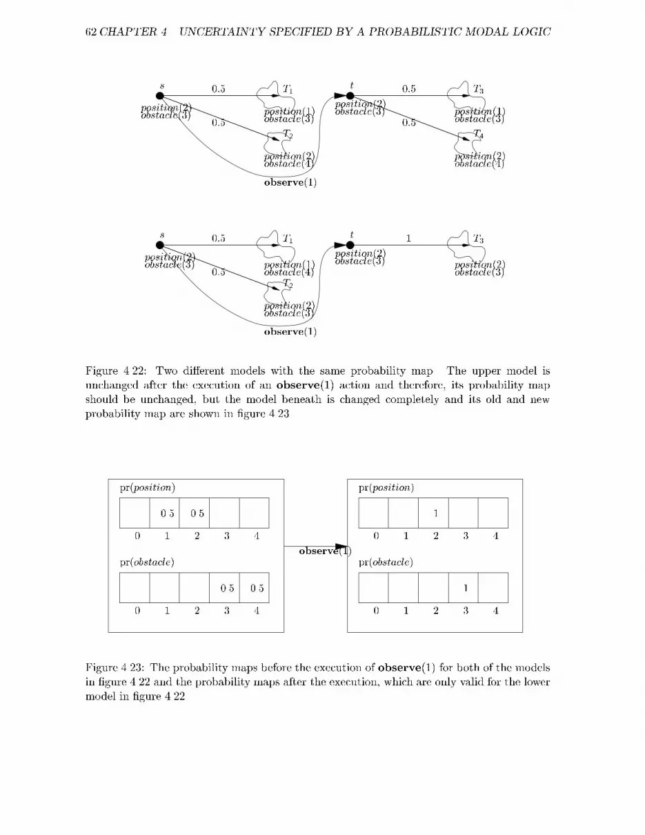
62CHAPTER 4. UNCERTAINTY SPECIFIED BY A PROBABILISTIC MODAL LOGICobserve(1)observe(1)

0:5 T1T2position(2) 0:5sobstacle(3) position(1)obstacle(4)position(2)obstacle(3)

0:5 T1T20:5 0:50:5 T3T4obstacle(3)1 T3position(2)

s tt

position(1)obstacle(3)position(2)obstacle(4) position(1)obstacle(3)position(2)obstacle(4)position(2)obstacle(3) position(2)obstacle(3)position(2)obstacle(3)

Figure 4.22: Two di�erent models with the same probability map. The upper model isunchanged after the execution of an observe(1) action and therefore, its probability mapshould be unchanged, but the model beneath is changed completely and its old and newprobability map are shown in �gure 4.23.observe(1)pr(obstacle)

pr(position)0.50.5 0.5

0.5 pr(position)pr(obstacle) 1

11 2 3 400 1 2 3 4 0 1 2 3 4

0 1 2 3 4Figure 4.23: The probability maps before the execution of observe(1) for both of the modelsin �gure 4.22 and the probability maps after the execution, which are only valid for the lowermodel in �gure 4.22.

4.6. IMPLEMENTATION 63s t1t2t3tn

�2�3�n�1

Figure 4.24: The general form of a model which is the result of probmap2model.This de�nition also de�nes a mapping from a model to a probability distribution as de�nedin de�nition 4.4.26. This depends on whether the probabilities of this proposition in the modelsum till one.To cope with probability maps as we did with our models, we also need the reversefunction probmap2model which de�nes a model using a probability map. As we said before,several functions of this type exists which satis�es for any probability map pms: pms =model2probmap(probmap2model(pms)). In the same way we choose to de�ne a probmap2model andtake a set of worlds, such that for each model MM and state s from this set the following holds:(MM; s) = probmap2model(model2probmap((MM; s))). The special property of the models in thisset is that all the propositions are independent of each other. Under this assumption, thereexists only one probmap2model function which meets our demands.De�nition 4.6.2 probmap2model : probmaps !WLet pms be the probability map of the mps p based on a k � l grid. We construct a modelMM in the following way: First create one state s; this is the current state the agent is in.Furthermore create states ti and de�ne the function �(ti) for i = 1 : : : 2kl, such that for eachstate ti one of the 2kl combinations of the k � l propositions is true. Create the relation R suchthat R(s; ti) for i = 1 : : : 2kl. De�ne Pr(s; t) = �(i;j)2f(i;j)2ZZ2j(MM;t)j=p(i;j)gpms(p)(i; j). Theresulting model is a very simple model which always looks like the one in �gure 4.24: onestate s and many direct successor states, but none of them has a successor themselves. Allthe states ti have probability �i = Pr(s; ti).Since any probability distribution is a probability map, this de�nition is also correct forprobability distributions.Now we are able to use probability maps as the basis for our reasoning. To derive aprobability map as the result of the execution of an action, we just have to calculate themodel from the probability map, transform this model with the function E and create aprobability map from the new model (see �gure 4.25):

64CHAPTER 4. UNCERTAINTY SPECIFIED BY A PROBABILISTIC MODAL LOGICpms pm0sE0(a)probmap2model(MM; s) (MM0; s0)model2probmapE(a)Figure 4.25: This diagram shows the way E0 is de�ned by equation (4.26).E0 : A! P(probmap)! P(probmap)E0(a)(fpmg) = model2probmap(E(a)(probmap2model(pms)))E0(a)(PMs) = fE0(a)(fpmsg)jpms 2 PMsg (4.26)For convenience, we allow the function E0(a) to take a single probability map as well assets, just like we did with E: E0(a)(pms) = E0(a)(fpmsg).Of course the derivation of a new probability map in this way would take just as much timeas it would have if we used only the models. Fortunately, we are able to derive E0 directly,but the result is not very attractive. It is, however, far more e�cient than the original.The e�ect of actions on probability mapsWe show the e�ect of a move action on a probability distribution of an mps like position,since this turns out to be the clearest mapping. The function E0(observe(y))(mps)(obstacle)can also be de�ned, but the result is rather complicated and it does not introduce somethingnew, therefore this function is not included here.Theorem 4.6.3 Suppose the agent is headed towards direction r. Suppose we have a proba-bility distribution of position, called pms. The new probability of position(z1; z2) is equal tothe sum of the probabilities of several starting positions times the probability that the agenthas actually moved the distance between this starting position and (z1; z2). The set of startingpositions is de�ned by X = f(round(z1 + (i� y) � cos(r)); round(z2 + (i� y) � sin(r)); i)ji 2 ZZg.Using this set and d = p(z1 � x1)2 + (z2 � x2)2, the new probability distribution is as follows:E0(move(y; tt))(pms)(position)(z1; z2) ==P(x1;x2)2X pms(x1; x2) � Pfreal move(d)jmoved(y)gBecause almost always Pfreal move(d)jmoved(y)g 6= 0 for just a small constant set of values,this mapping is linear in the size of the probability distribution, in terms of the beginning ofthis section: n �m.ProofLet (z1; z2) be given. Consider the probability of position(z1; z2) after the execu-tion ofmove(y; tt). This probability is equal to the probability of the set of stateswhich validates this formula. Simple mathematics tells us that for this set of statesthe following holds: 8i 2 ZZ9zs 2 ZZ2 : (z1 = zs1 + round((y + i) � cos(r))) ^ (z2 =zs2+round((y+i) �sin(r))). Using de�nition 4.5.5 we conclude that the zs's de�nedfor each i 2 ZZ represent the di�erent starting positions before the move(y).

4.6. IMPLEMENTATION 65

Figure 4.26: The Pioneer 1 with a camera.By theorem 4.4.18 we know that the probabilities for the sets of states de�nedby all the zs's are calculated by multiplying the probability of the original setof states, position(zs1; zs2), with the probability that the agent has really movedto the new position de�ned by the new set of states, Pfreal move(d)jmoved(y)gwith d = p(z1 � zs1)2 + (z2 � zs2)2.So the probability of position(z1; z2) after the move is equal to the sum ofall the probabilities of the sets of states position(zs1; zs2) as de�ned above. Thisproves the theorem.End of Proof4.6.2 A Pioneer in the real worldWe started this research to try to �nd a way to model the reasoning of a real robot in arealistic way. Only one way exists to prove that our language as proposed in this chapter issuited for this purpose. The language should be implemented on a real robot and should beused to control this robot. In this subsection we summarize a couple of issues that will arisewhen implementing this language on a Pioneer [Int].A Pioneer 1 is a mobile robot from ActivMedia. The most simple model has two largewheels and one small one. The two large ones can be controlled independently to turn thePioneer. This robot also has seven sonar sensors: one at the left side, one at the right sideand �ve at the front in slightly di�erent angles. This robot can be seen in �gure 4.26. Inaddition to the sonars, this Pioneer also has a camera, but we only use the sonars to test ourlanguage. Sonar sensors are one of the most noisiest sensors available, so this robot is a verygood test subject.

66CHAPTER 4. UNCERTAINTY SPECIFIED BY A PROBABILISTIC MODAL LOGICThe following problems immediately arise when trying to �t our language to this realworld robot.� We have to de�ne the size of the environment and the size of one cell in a grid. Theproduct of these values de�nes the size of the probability maps and thus the speed ofthe calculations, but if the size of the environment is too small, the agent will at somepoint cross its boundaries and be unable to store its observations. And if the size ofone cell is too large, the agent will be unable to detect narrow corridors. A cell size ofabout 1 cm seems accurate enough and for indoor environments, a size between 10 and100 m square should be su�cient.� In this chapter we assumed the size of the robot to be less than the size of one cell ofthe grid, but in general it is very unlikely someone should use such large cells or such asmall robot. Our results, however, are easily convertable to a multi-cell robot situation.We should change only two things. First, the interpretation of position(z) should be:the center of the robot is at position z. Second, the interpretation of a failed move(move(y;�)) should change: instead of assuming an obstacle to be at position z + y,we should assume an obstacle to be at position z + y + nose size � 1, with nose sizebeing the distance from the center of the robot to the nose.� We also assumed that the shape of the robot is a perfect circle, but the shape of thePioneer isn't. However, with a few simple changes our language can cope with thisproblem. The turn should be executed as if the Pioneer was a perfect circle with adiameter equal to the length of the Pioneer, but the move should conclude there areno obstacles at a path behind itself with the width of the Pioneer.� The Pioneer has more than one sonar. This is no real problem. There will just be a lotof observe actions within few seconds.� The sonars are placed in di�erent angles and positions relative to the robot's origin, sowe should de�ne a new E(observe) which accounts for a relative position and direction.This is rather straightforward, because we could treat this as if the agent has movedand turned to that relative position.� A real robot is able to turn and move simultaneously. After some geometrical exercisesit should be possible to de�ne a curved move or something like that. However, the usefor all this hard work is limited. The Pioneer can do almost as much without thesestrange moves as with a curved move, except for some rare situation in which a curvedcorridor with the width of the Pioneer exists in the environment.� We assumed a move to be noisy in the distance travelled, but a move can also disturbthe direction in which the robot is turned. We should de�ne a new E(move) to accountfor this change in direction and the changes in position which are the consequence ofthis change in direction. Because the noise will be larger when the moved distance isgreater, the e�ect of a move will be that the new positions within the outer arc of asector get a greater probability.� Probability maps do not have the same expressibility as the Kripke models. Because weignored the dependence between obstacle and position, we must introduce another wayto couple these propositions. This way has been used by several other methods. It is

4.6. IMPLEMENTATION 67called self-relocation. Using the current readings of the sonars and the global obstacleprobability map, the position map is updated, such that the probabilities are moreconcentrated around the most probable position.� We never mentioned anything about planning in this chapter. This chapter concentratedon representing the knowledge of an agent, but to create a complete control system fora Pioneer we should also develop a system to plan ahead and to take decisions based onthe current knowledge of the environment. An article of Brafman and others [BLMS97]on motion planning under uncertainty might be a good start to introduce planning inthis language.� We mapped the real world to a grid. This method is often used and worked quite well,but it still would be very neat if real values could be used instead of grid cell coordinates.� Two other aspects of the real world haven't been accounted for. When a sonar sendsout a signal it is possible that the signal is not re ected directly back to the robot.This is called specular re ection. When the robot does not move and gets multipletimes exactly the same information, it tells us very little. In our approach we assumedthat more times the same information increases the probability of this information. Ingeneral this is not true because of specular re ection. This problem is solved probablyas well as possible by Konolige [Kon96] [Kon97].As can be seen from the length of this list, we have not �nished this quest for a logic-drivenrobot yet.

68CHAPTER 4. UNCERTAINTY SPECIFIED BY A PROBABILISTIC MODAL LOGIC

Chapter 5Discussion and future work5.1 Comparing to related workIn this chapter we �rst compare the logical language we introduced in chapter 4 with thework described in chapters 1, 2 and 3. We start with the methods from chapter 2, which areall implemented and working. Unfortunately, these methods do not result in correct behaviorin all situations. By testing and trial and error it can be established when they do or do notwork. This approach is not only very time consuming, it also gives very few insights in themobile robot control-problem. Exactly the collecting of these insights is the goal of manylogical approaches.Shanahan's method as described shortly in section 3.1 is such a logical approach. Com-paring to ours, we see a few advantages of his method the major being that continuous changeis incorporated and that a working implementation exists. However, he works with sensorsthat are not noisy and no suggestions are made how to handle the uncertainty introducedby for example sonars. Existing methods which includes reasoning about multiple agents,opportunities and abilities [vLvdHM98] are based on modal logic, like our approach. So, weget these extentions almost for free. Shanahan uses a simpli�cation of the circumscriptiveevent calculus [Sha95] and probably will have to do some more work to include these notions.The situation calculus approach of Bacchus, Halpern and Levesque as described in sec-tion 3.2 is much more the same as our approach. Situation calculus also uses a sort of possibleworld semantics like modal logic, except for the history of situations which is implicit in asituation of the situation calculus. Uncertainty is included by assigning a probability to situ-ation transitions, almost in the same way as we do. However, in their article in 1995 [BHL95],their approach did not include noisy e�ectors like we took care of in section 4.4.3. Anotherdi�erence is that we did pay some attention to the extension of the application of our logicallanguage to the second dimension (see section 4.5) and we did pay attention to some otherimplementation issues (section 4.6). So our language is not just a translation of their approachfrom situation calculus to modal logic, so that it is easier to combine with other modalities;it is really far more extensive.Halpern did also introduce a logical language based on modal logic which includes prob-abilities as summarized in section 3.3. At �rst, this language seems even more the same asours, because both approaches use modal logic. However, he did not introduce actions andtheir results and the way uncertainty should be handled in connection with mobile robots isnot taken care of in his article. Therefore everything starting from section 4.3 is new from69

70 CHAPTER 5. DISCUSSION AND FUTURE WORKthe viewpoint of a logic of knowledge, probability and time [Hal97].Finally we would like to compare our logical language to another logical language based onmodal logics, the KARO-framework as summarized in section 3.4. Although this frameworkis made to �t an agent and even multiple agents, very few adaptations are made to make it�t to a real-world robot. The results of actions are very important in this framework, butprobabilities are not introduced, so the unreliability of the results of actions cannot be stated.Therefore no attention is paid to problems concerning noisy sensors and noisy e�ectors. Itmight be a could idea to incorporate our logical language in this framework, so the beni�tsof both are combined.5.2 DiscussionModal logic is certainly powerful enough to specify both actions and uncertainty. It is possibleto combine these modalities with others like abilities and opportunities [vLvdHM98] and toextend it to a multi-agent approach to create a very complete and powerful language toexpress statements about agents. It should even be possible to de�ne rules in this languagewhich specify avoidance behavior or planning as described in chapter 1. In fact the wholecontrol system could be implemented in this language. Of course these are interesting topicsfor future research, but before starting to use this language to control an agent, it is wiseto understand the problems which arise when trying to implement such a language and theaccompanying mechanism to perform the reasoning automatically.The most di�cult of these problems is the exponential size of the models in terms ofthe number of propositions. The solution we presented in section 4.6 is rather ad hoc andloses one of the nicest properties of a modal logic. The possible worlds implicitly de�nethe dependence between propositions and in this solution we supposed all propositions to beindependent. Maybe another e�cient solution exists which conserves more of the propertiesof modal logic.5.3 Future researchAs should be clear from section 4.6.2 a lot of research still can be done in this area. First,we would like to pay some more attention to the goal of the logical language as proposed inthis document. Should it only be used to describe agents and their actions on a meta-levelor should it also be used to control the agent in real-time? If so, we have to �nd a way toimplement this language e�ciently and then it is also very interesting to see how rules onhow to control the agent can be stated in this language.Another interesting topic is how opportunities and abilities can be introduced or howthis language can be extended to use it for multi-agent systems. Some of the problemsmentioned in 4.6.2 require some research and �nally we would like to have an axiomatizingfor our language, so we will be able to prove statements in our language without translatingeverything to the models. Probably we will encounter the frame-problem here and have to�nd out which of the existing solutions can be used to solve it in our case.We think this research is one step more towards a method using logic to describe agentsand agents' behaviors in a realistic and detailed way.

Bibliography[BFHS96a] W. Burgard, D. Fox, D. Hennig, and T. Schmidt. Estimating the ab-solute position of a mobile robot using position probability grids. InProceedings of the Thirteenth National Conference on Arti�cial Intelli-gence and the Eighth Innovative Applications of Arti�cial Intelligence Con-ference, pages 896{901, Menlo Park, 1996. AAAI Press / MIT Press.http://www.informatik.uni-bonn.de/~fox/rhino/publications.html.[BFHS96b] W. Burgard, D. Fox, D. Hennig, and T. Schmidt. Position tracking withposition probability grids. In Proceedings of the 1st Euromicro Workshopon Advanced Mobile Robots (EUROBOT'96), Germany, 1996. Kaiserslautern.http://www.informatik.uni-bonn.de/~fox/rhino/publications.html.[BHL95] F. Bacchus, J.Y. Halpern, and H.J. Levesque. Reasoning about noisy sensors inthe situation calculus. In Proceedings of the 14th International Joint Conferenceon Arti�cial Intelligence, pages 1933{1940, 2929 Campus Dr., Suite 260, SanMateo, CA, 94403, USA, 1995. Morgan-Kaufmann.[BLMS97] R.I. Brafman, J.-C.L. Latombe, Y. Moses, and Y. Shoham. Ap-plications of a logic of knowledge to motion planning under un-certainty. Journal of the ACM, 44(5):633{668, september 1997.http://robotics.stanford.edu/users/brafman/publications.html.[FHMV95] R. Fagin, J.Y. Halpern, Y. Moses, and M.Y. Vardi. Reasoning about Knowledge.MIT Press, Cambridge, Mass., 1995.[Gn96] J. Ga�os and A. Mart�� n. Mobile robot localization using fuzzy maps. InA. Ralescu and T. Martin, editors, Fuzzy Logic in Arti�cial Intelligence, volume1188 of Lecture Notes on Arti�cial Intelligence, pages 207{224. Springer Verlag,1996.[Gol82] R. Goldblatt. Axiomatizing the Logic of Computer Programming, volume 130of Lecture Notes on Computer Science. Springer Verlag, New York, NY, USA,1982.[Gol86] R. Goldblatt. Logics of Time and Computation, volume 7 of Center for the Studyof Language and Information lecture notes. Center for the Study of Languageand Information, Stanford, 1986.[Hal97] J.Y. Halpern. A logical approach to reasoning about uncertainty: a tutorial.In X. Arrazola, K. Korta, and F.J Pelletier, editors, Discourse, Interaction andCommunication. Kluwer, 1997. http://www.cs.cornell.edu/home/halpern.71

72 BIBLIOGRAPHY[Int] Real World Interface. Mobile robots from activmedia and real world interface.http://www.activmedia.com/RealWorld/.[KL95] G.N. Kartha and V. Lifschitz. A simple formalization of actions using cicum-scription. In Proceedings of the International Joint Conference on Arti�cialIntelligence 95, pages 1970{1975, 1995.[KLC98] L.P. Kaelbling, M.L. Littman, and A.R. Cassandra. Planning and actingin partially observable stochastic domains. Arti�cial Intelligence, 101, 1998.http://www.cs.brown.edu/~lpk/pomdp-ai.ps.[KMRS97] K. Konolige, K.L. Myers, E.H. Ruspini, and A. Sa�otti. The Saphira architec-ture: A design for autonomy. Journal of experimental & theoretical arti�cialintelligence: JETAI, 9(1):215{235, 1997.[Kon96] K. Konolige. A re�ned method for occupancy grid interpretation. In Proceed-ings of the International Workshop on Reasoning with Uncertainty in Robotics(RUR-95), volume 1093 of Lecture Notes on Arti�cial Intelligence, pages 338{352. Springer Verlag, 1996.[Kon97] K. Konolige. Improved occupancy grids for map building. Autonomous Robots,4(4), October 1997.[KP81] D. Kozen and R. Parikh. An elementary proof of completeness for pdl. Theo-retical Computer Science, 14:113{118, 1981.[Lau98] J.-P. Laumond, editor. Robot Motion Planning and Control, volume 229 ofLecture Notes in Control and Information Sciences. Springer Verlag, 1998.[ME85] H.P. Moravec and A.E. Elfes. High resolution maps from wide angle sonar. InProceedings of the IEEE International Conference on Robotics and Animation,pages 116{121. IEEE Computer Society Press, 1985.[Mey89] J.-J.Ch. Meyer. Using programming concepts in deontic reasoning. InR. Bartsch, J. van Benthem, and P. van Emde Boas, editors, Seman-tics and Contextual Expression, pages 117{145. FORIS Publications, Dor-drecht/Riverton, 1989.[Mor88] H.P. Moravec. Sensor fusion in certainty grids for mobile robots. AI Magazine,pages 61{74, Summer 1988.[MvdH95] J.-J.Ch. Meyer and W. van der Hoek. Epistemic Logic for AI and ComputerScience, volume 41 of Cambridge Tracts in Theoretical Computer Science. Cam-bridge University Press, 1995.[PNDW96] D. Pagac, M.N. Nebot, and H. Durrant-Whyte. An evidential approach toprobabilistic map-building. In Reasoning with Uncertainty in Robotics, volume1093 of Lecture Notes on Arti�cial Intelligence, pages 164{170. Springer Verlag,1996. http://mecharea.me.su.oz.au/papers/dan-ICRA96/icra96.htm.

BIBLIOGRAPHY 73[Saf97] A. Sa�otti. The uses of fuzzy logic in autonomous robot navi-gation: a catalogue raisonn�e. Soft Computing, 1(4):180{197, 1997.http://iridia.ulb.ac.be/saffiotti/papers.html.[Sha76] G. Shafer. A mathematical theory of evidence. Princeton University Press, 1976.[Sha95] M.P. Shanahan. A circumscriptive calculus of events. Arti�cial Intelligence,77:249{284, 1995.[Sha96a] M.P. Shanahan. A Logical Account of the Common Sense Informatic Situationfor a Mobile Robot. 1996. http://www.dcs.qmw.ac.uk/~mps/pubs.html. Thisunpublished work is a combination of [Sha96b] and [Sha96c].[Sha96b] M.P. Shanahan. Noise and the common sense informatic situation for a mobilerobot. In Proceedings of AAAI 96, pages 1098{1103, 1996.[Sha96c] M.P. Shanahan. Robotics and the common sense informatic situation. In Pro-ceedings of ECAI 96, pages 684{688, 1996.[Sho93] Y. Shoham. Agent oriented programming. Journal on Arti�cial Intelligence,60(1):51{92, 1993.[SKR95] A. Sa�otti, K. Konolige, and E.H. Ruspini. A multivalued logic approach tointegrating planning control. Arti�cial Intelligence, 76(1{2):481{526, 1995.[SW96] A. Sa�otti and L.P. Wesley. Perception-based self-localization using fuzzy loca-tions. In Reasoning with Uncertainty in Robotics, volume 1093 of Lecture Noteson Arti�cial Intelligence, pages 368{385. Springer Verlag, 1996.[TBF97] S. Thrun, B. Burgard, and D. Fox. A probabilistic approach to concurrentmapping and localization for mobile robots. Machine Learning / AutonomousRobots, 1997. http://www.cs.cmu.edu/~thrun/papers/index.html.[Tri82] K. Trivedi. Probability & Statistics with reliability, queuing and Computer Sci-ence applications. Prentice-Hall, Inc., Eaglewood Cli�s, 1982.[vB88] J. v. Benthem. A manual of intensional logic, volume 1 of Center for the Studyof Language and Information lecture notes, pages 49{53. Center for the Studyof Language and Information, Stanford, 1988.[vdH92] W. van der Hoek. Modalities for Reasoning about Knowledge and Quantities.PhD thesis, University of Amsterdam, Amsterdam, 1992.[vL96] B. van Linder.Modal Logics for Rational Agents. PhD thesis, Utrecht University,Utrecht, 1996.[vLvdHM98] B. van Linder, W. van der Hoek, and J.-J.Ch. Meyer. Formalizing abilities andopportunities of agents. Fundamental Informaticae, 34(1,2):53{101, 1998.