Spectrophotometric variable selection by mutual information

www.elsevier.com/locate/chemolab

Chemometrics and Intelligent Laboratory Systems 74 (2004) 243–251

Spectrophotometric variable selection by mutual information

N. Benoudjita,1, D. Franc�oisb,2, M. Meurensc,3, M. Verleysena,*,4

aUniversite catholique de Louvain (UCL), Microelectronics Laboratory (DICE), Place du Levant 3, 1348 Louvain-la-Neuve, BelgiumbCESAME, Avenue Georges Lemaitre 4, B-1348 Louvain-la-Neuve, Belgium

cSpectrophotometric Laboratory (BNUT), Place Croix du Sud 2/8, B-1348 Louvain-la-Neuve, Belgium

Received 3 December 2003; received in revised form 27 January 2004; accepted 21 April 2004

Available online 24 July 2004

Abstract

Spectrophotometric data often comprise a great number of numerical components or variables that can be used in calibration models.

When a large number of such variables are incorporated into a particular model, many difficulties arise, and it is often necessary to reduce the

number of spectral variables. This paper proposes an incremental (Forward–Backward) procedure, initiated using an entropy-based criterion

(mutual information), to choose the first variable. The advantages of the method are discussed; results in quantitative chemical analysis by

spectrophotometry show the improvements obtained with respect to traditional and nonlinear calibration models.

D 2004 Elsevier B.V. All rights reserved.

Keywords: Spectrophotometric variable selection; Mutual information; Spectrophotometry

1. Introduction product, from spectral data measured on various wave-

The infrared spectra of agricultural and food products

contain information that presents an analytical interest.

However, the extraction of this information is not immediate

and requires almost always a rather complex mathematical

treatment. Indeed, the spectra are the result of an interaction

of light with matter that cannot completely be described

from a theoretical point of view.

This paper focuses particularly on the application of

chemometrics in the field of analytical chemistry. Chemo-

metrics (or multivariate analysis) consists of finding a

relationship between two groups of variables, often called

dependent and independent variables. In infrared spectros-

copy for instance, chemometrics consists of the prediction

of a quantitative variable (the obtention of which is delicate,

requiring a chemical analysis and a qualified operator), such

as the concentration of a component present in the studied

0169-7439/$ - see front matter D 2004 Elsevier B.V. All rights reserved.

doi:10.1016/j.chemolab.2004.04.015

* Corresponding author. Tel.: +32-10-47-25-51; fax: +32-10-47-25-98.

E-mail addresses: [email protected] (N. Benoudjit),

[email protected] (D. Franc�ois), [email protected]

(M. Meurens), [email protected] (M. Verleysen).1 Tel.: +32-10-47-25-40; fax: +32-10-47-25-98.2 Tel.: +32-10-47-80-02; fax: +32-10-47-21-80.3 Tel.: +32-10-47-37-26; fax: +32-10-47-37-28.4 Michel Verleysen is a Senior Research Associate of the Belgian

F.N.R.S. (National Fund For Scientific Research).

lengths or wave numbers (several hundreds, even several

thousands).

From a chemometric point of view, the spectrum

obtained in infrared spectroscopy is a complex function that

depends on both the physical and chemical properties of the

sample [1], and has remarkable characteristics that require

specific methods for their treatment.

The spectrophotometric data may often comprise more

independent variables (spectral data) than observations

(spectra or samples). This case is rather less encountered

in other applications of statistics. Collinearity of the inde-

pendent variables is typical for spectrophotometric data, that

is, certain independent variables can be practically repre-

sented as a linear combination of other independent ones;

this is the source of many problems in direct application of

many statistical methods, such as the multiple linear regres-

sion (MLR) [2–6]. Studies have shown that if collinearity is

present among variables, the prediction results can get poor

(see for example Refs. [4,7]). This limitation has promoted

other alternative linear methods to offset the problems

generated by the strong redundancy between variables.

Several alternatives that are able to adapt to this collinearity

were developed, such as stepwise multiple linear regression

(SMLR) [3,8–11], principal component regression (PCR)

[5,6,10,12,13], partial least square regression (PLSR)

[3,6,10,12–16], and so forth.

N. Benoudjit et al. / Chemometrics and Intelligent Laboratory Systems 74 (2004) 243–251244

In analytical chemistry, a lot of linear calibration methods

(mentioned above) are applied to solve quantitative prob-

lems with the argument that the relation between the chem-

ical composition and the measured signal is linear [17].

However, there are many situations where nonlinearity is

present. For instance, Miller [18] discusses important sour-

ces of nonlinearity in near-infrared spectroscopy, namely

� deviations from the Beer–Lambert law, which are typical

of highly absorbing samples;� nonlinear detector responses;� drifts in the light source;� interactions between analytes;� nonlinearity between diffuse reflectance/transmittance

data and chemical data.

When the nonlinearity is significant, one can use truly

nonlinear calibration techniques, for example, artificial

neural networks (ANN).

The purpose of this study is to predict the concentration

(dependent variable) of analyte present in a studied product

from independent variables, which are spectral data mea-

sured on various wavelengths. Because spectrophotometric

data have specific characteristics (a.o. collinearity), it is

necessary to select independent variables among the candi-

dates to build a still suitable model with only few variables.

The objective of variable selection is three-fold: improving

prediction performances, providing faster and more cost-

effective prediction, and providing a better understanding of

the underlying process that generated the data [19].

In Ref. [20], we proposed a procedure for spectral data

selection in infrared spectroscopy based on the combination

of three principles: linear or nonlinear regression, incremen-

tal procedure for variable selection, and use of a validation

set. This procedure allows on one hand to benefit from the

advantages of nonlinear methods to predict chemical data

(there is often a nonlinear relationship between dependent

and independent variables), and on the other hand to avoid

the overfitting phenomenon, one of the most crucial prob-

lems encountered with nonlinear models. In this paper, we

suggest to improve this method by a judicious choice of the

first spectral data, which have a very high influence on the

selection of other variables and on the final performances of

the prediction.

In the first iteration of the incremental procedure, a

model is built with only one independent variable. Although

the intrinsic dimensionality of the spectra is less than the

hundreds of variables used to describe them, one variable is

definitely not enough to rightly characterize a spectrum. As

a consequence, building a regression model with only one

independent variable hardly makes sense; its expected

results are very poor and should not be used ‘‘as-is’’ to

initiate the incremental procedure. That is why we suggest

not to build any model in the first iteration but rather trust a

model-independent criterion for the choice of the first

spectral variable.

The idea is to use a measure of the mutual informa-

tion between the spectral data (independent variables)

and the concentration of analyte (dependent variable) to

select the first variable; indeed, this measure allows to

identify the variable (spectral data) having the highest

relation to the analyte. Once the first variable is selected

the incremental procedure (forward–backward selection,

FBS) [20] is used to select the next spectral variables.

If the idea of using a mutual information criterion for

the choice of the other spectral data can also seem

relevant, its implementation becomes more and more

difficult when the number of selected variables increases.

Indeed, we will see in the next section that estimating the

mutual information between a group of k variables and

another one requires the estimation of a (k + 1)-dimension-

al joint probability density function (pdf). As k increases,

that estimation gets less and less accurate because of the

lack of sufficient number of examples and the inherent so-

called ‘‘empty space phenomenon’’ [21]. We will thus

limit the use of mutual information criterion to the crucial

choice of the first spectral variable; we will see in the

Results section that it is advantageous to combine the

two approaches.

Furthermore, the variable selected by mutual information

can have a good interpretation from the spectrochemical

point of view and does not depend on the data distribution in

the training and validation sets. On the other hand, the

traditional chemometric linear methods such as PCR or

PLSR produce new variables that do not have an obvious

interpretation from the spectrochemical point of view.

In this work, we will first explain how mutual informa-

tion can be used to assess the importance of each variable

(spectral data) with respect to the calibration model. Then,

we will propose the new variable selection method based on

the combination of two ideas: the mutual information to

select the first variable and then the application of the FBS-

radial basis function network (RBFN) method [20] to select

the next ones. Lastly, we will present a comparison of

prediction results between the improved and PCR, PLSR,

and FBS-RBFN methods.

2. Mutual information

In this section, we will explain how the mutual informa-

tion can be used to assess the relevance of an independent

variable to predict a dependent variable.

2.1. Definitions

The first goal of a prediction model is to minimize the

uncertainty on the dependent variable. A good formalization

of the uncertainty of a random variable is given by Shannon

and Weaver’s [22] information theory. While first devel-

oped for binary variables, it has been extended to contin-

uous variables.

N. Benoudjit et al. / Chemometrics and Intelligent Laboratory Systems 74 (2004) 243–251 245

The uncertainty of a random variable y with values v in a

finite set D can be measured by its entropy H:

HðyÞ ¼ �XvaD

Pðy ¼ vÞ � logPðy ¼ vÞ: ð1Þ

To illustrate this concept, let us suppose that in an

extreme case all values v a D have null probability except

one, say v*, which has a probability equal to 1, that is,

Pðy ¼ vÞ ¼1 if v ¼ v*

0 otherwise:

8<: ð2Þ

The entropy is thus H(y) = 0; indeed there is absolutely

no uncertainty since y always has value v*.

Suppose on the other hand that all values in D are

equiprobable:

bvaD : Pðy ¼ 0Þ ¼ 1

#Dð3Þ

Uncertainty is then maximal since no value is more

probable than others. In this case, it is possible to show

that the entropy is maximal too: H(y) = log #D.

When the value of another variable xi with values vV inDV is known, one can define the conditional entropy:

Hðy j xiÞ ¼ �X

vVaDV

Pðxi ¼ vVÞXvaD

Pðy ¼ v j xi ¼ vVÞ

� logPðy ¼ v j xi ¼ v VÞ: ð4Þ

This represents the uncertainty on y when xi is known.

The difference between the uncertainty on y and the

uncertainty on the same variable knowing xi is called the

mutual information between xi and y:

Iðy; xiÞ ¼ HðyÞ � Hðy j xiÞ ð5Þ

It represents the decreasing of uncertainty on y when xi is

known. Reexpressing P(y = vjxi = vV) as P(y = v^xi = vV)/P(xi = vV), one can show that

Iðy; xiÞ ¼X

vaD;vVaDV

Pðy ¼ v ^ xi ¼ vVÞ

� logPðy ¼ v ^ xi ¼ vVÞ

Pðy ¼ vÞ � Pðxi ¼ vVÞ ð6Þ

This formulation shows that the mutual information

between xi and y is zero if and only if xi and y are

statistically independent. Furthermore, the mutual informa-

tion is not affected by any variable transformation and does

not make any assumption on the underlying relationship

between xi and y.

The concepts of entropy, conditional entropy and mutual

information, can be extended to the continuous case (set D

of infinite size).

The uncertainty of a continuous random variable y with

probability density function (pdf) f (y) is given by:

HðyÞ ¼ �Z

f ðyÞlog f ðyÞdy ð7Þ

and the conditional entropy when xi is known:

Hðy j xiÞ ¼�Z

f ðxiÞZ

f ðy j xiÞ � log f ðy j xiÞdydxi: ð8Þ

The mutual information between variables y and xi may

be expressed by [23,24]:

I ¼Z

hðxi; yÞ � log hðxi; yÞf ðxiÞ � gðyÞ

dxidy; ð9Þ

where f (xi) and g(y) are the marginal probability densities of

variables xi and y, respectively, and h(xi, y) is the joint

probability density function of xi and y.

Since

f ðxiÞ ¼Z

hðxi; yÞdy; ð10Þ

and

gðyÞ ¼Z

hðxi; yÞdxi; ð11Þ

we only need to estimate h(xi, y) to estimate the mutual

information between xi and y.

2.2. Estimation of the mutual information

As we saw in the previous section, estimating the mutual

information between xi and y requires the estimation of the

joint probability density function of xi and y. This estimation

has to be carried on the data set. Histogram- and kernel-

based pdf estimations are among the most commonly used

[25]. In this study, we used histogram estimation for its

reduced computation requirements.

Because we need to estimate the joint density h(y, xi), we

must construct a bidimensional histogram {hk,j}(1V kVm,

1V jV n) approximating the bidimensional pdf surface with

a set of rectangular tiles (cells) {[ak, ak + 1]� [bj, bj + 1]}.

The procedure starts by building the set of tiles as a

bidimensional grid [a1,. . ., am + 1]� [b1,. . ., bn + 1] spanning

the Cartesian product of the respective ranges of xi and y.

Then, the number of pairs (xi, y) that fall into a particular

cell [ak, ak + 1]� [bj, bj + 1] has to be counted:

hk; j ¼ #fðxi; yÞAakVxi < akþ1 and bj V y < bjþ1g: ð12Þ

The sizes (ak + 1� ak) and (bj + 1� bj) of the cells are

important parameters that have to be chosen carefully. If the

cells are too large, the approximation will not be precise

enough; if they are too small, most of them will be empty

and the approximation will not be sufficiently smooth. Even

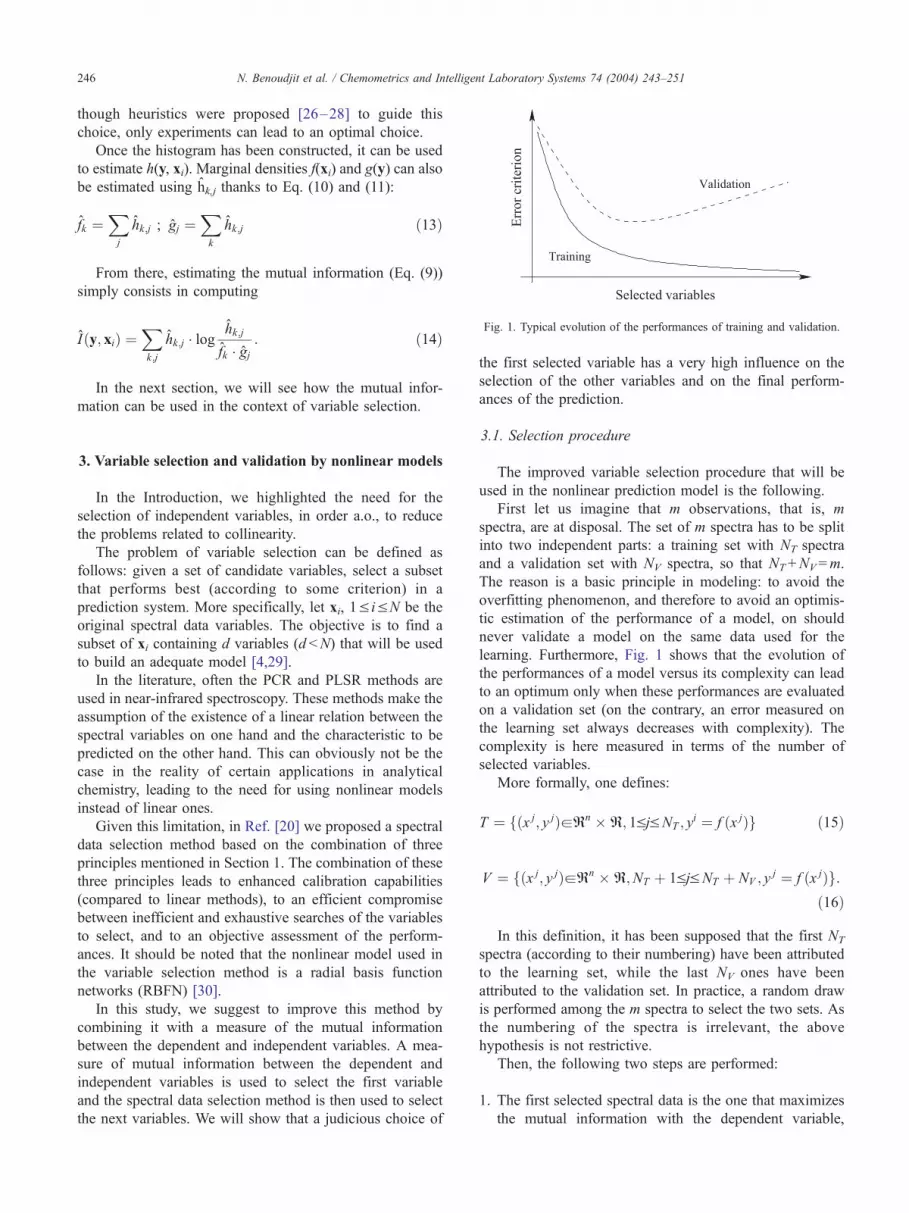
Fig. 1. Typical evolution of the performances of training and validation.


though heuristics were proposed [26–28] to guide this

choice, only experiments can lead to an optimal choice.

Once the histogram has been constructed, it can be used

to estimate h(y, xi). Marginal densities f(xi) and g(y) can also

be estimated using hk,j thanks to Eq. (10) and (11):

fk ¼Xj

hk;j ; gj ¼Xk

hk;j ð13Þ

From there, estimating the mutual information (Eq. (9))

simply consists in computing

Iðy; xiÞ ¼Xk;j

hk;j � loghk;j

fk � gj: ð14Þ

In the next section, we will see how the mutual infor-

mation can be used in the context of variable selection.

3. Variable selection and validation by nonlinear models

In the Introduction, we highlighted the need for the

selection of independent variables, in order a.o., to reduce

the problems related to collinearity.

The problem of variable selection can be defined as

follows: given a set of candidate variables, select a subset

that performs best (according to some criterion) in a

prediction system. More specifically, let xi, 1V iVN be the

original spectral data variables. The objective is to find a

subset of xi containing d variables (d <N) that will be used

to build an adequate model [4,29].

In the literature, often the PCR and PLSR methods are

used in near-infrared spectroscopy. These methods make the

assumption of the existence of a linear relation between the

spectral variables on one hand and the characteristic to be

predicted on the other hand. This can obviously not be the

case in the reality of certain applications in analytical

chemistry, leading to the need for using nonlinear models

instead of linear ones.

Given this limitation, in Ref. [20] we proposed a spectral

data selection method based on the combination of three

principles mentioned in Section 1. The combination of these

three principles leads to enhanced calibration capabilities

(compared to linear methods), to an efficient compromise

between inefficient and exhaustive searches of the variables

to select, and to an objective assessment of the perform-

ances. It should be noted that the nonlinear model used in

the variable selection method is a radial basis function

networks (RBFN) [30].

In this study, we suggest to improve this method by

combining it with a measure of the mutual information

between the dependent and independent variables. A mea-

sure of mutual information between the dependent and

independent variables is used to select the first variable

and the spectral data selection method is then used to select

the next variables. We will show that a judicious choice of

the first selected variable has a very high influence on the

selection of the other variables and on the final perform-

ances of the prediction.

3.1. Selection procedure

The improved variable selection procedure that will be

used in the nonlinear prediction model is the following.

First let us imagine that m observations, that is, m

spectra, are at disposal. The set of m spectra has to be split

into two independent parts: a training set with NT spectra

and a validation set with NV spectra, so that NT+NV=m.

The reason is a basic principle in modeling: to avoid the

overfitting phenomenon, and therefore to avoid an optimis-

tic estimation of the performance of a model, on should

never validate a model on the same data used for the

learning. Furthermore, Fig. 1 shows that the evolution of

the performances of a model versus its complexity can lead

to an optimum only when these performances are evaluated

on a validation set (on the contrary, an error measured on

the learning set always decreases with complexity). The

complexity is here measured in terms of the number of

selected variables.

More formally, one defines:

T ¼ fðx j; y jÞaRn �R; 1VjVNT ; y

i ¼ f ðx jÞg ð15Þ

V ¼ fðx j; y jÞaRn �R;NT þ 1VjV NT þ NV ; y

j ¼ f ðx jÞg:ð16Þ

In this definition, it has been supposed that the first NT

spectra (according to their numbering) have been attributed

to the learning set, while the last NV ones have been

attributed to the validation set. In practice, a random draw

is performed among the m spectra to select the two sets. As

the numbering of the spectra is irrelevant, the above

hypothesis is not restrictive.

Then, the following two steps are performed:

1. The first selected spectral data is the one that maximizes

the mutual information with the dependent variable,


according to the estimation method detailed in the

previous section.

2. Other spectral data are selected according to the

forward–backward selection procedure with RBF net-

works (FBS-RBFN) [20]: Forward selection: once k variables have been selected

(k = 1 in the first iteration), p� k models with k + 1

variables (the selected k and, respectively, each of the

other ones) are built and compared according to an

error criterion on a validation set; the variable

corresponding to the minimum of the error criterion

is added. The ‘forward’ process is repeated for k = 2,

3,. . ., until the value of the error criterion (on the

validation set) increases. Backward selection: it consists of eliminating the

least significant spectral data already selected in the

‘forward’ stage. If q spectral variables were selected

after the ‘forward’ stage, q models are built by

removing, respectively, one of the selected variables.

Fig. 2. Near-infrared reflectance

The error criterion on a validation set is calculated

for each of these models, and the one with the

lowest error is selected. Once the model is chosen,

we compare its error to the error of the model

obtained at the preceding stage. If the error criterion

corresponding to the new model is lower, then the

selected spectral variable is not significant and may

be removed. The process is then repeated on the

remaining spectral variables. The backward selection

is stopped when the lowest error among all models

calculated at a specific step is higher than the error

at the previous step.

It should be noted that during Step 1, we only need the

training set since the computation of the mutual information

does not require the estimation and the comparison of

models. On the other hand, for Step 2, it is necessary to

use other data (validation set) independent from the training

set for the computation of the error criterion.

spectra of three data sets.

Table 1

Number of selected variables and their corresponding NMSEV for the three

data sets

Data set Calibration model Number of variables NMSEV

Orange juice PCR 42 0.2596

PLSR 16 0.2435

FBS-RBFN 13 0.0703

MI + FBS-RBFN 36 0.0313

Milk powder PCR 10 0.9250

PLSR 7 0.8758

FBS-RBFN 6 0.5309

MI + FBS-RBFN 18 0.4816

Apple PCR 7 0.6721

PLSR 4 0.6029

FBS-RBFN 8 0.2787

MI + FBS-RBFN 12 0.2321


3.2. Error criterion

As mentioned in Step 2 above, the respective errors of

several models must be evaluated on data independent from

the one used for learning, that is, data from a validation set.

Fig. 3. Spectrum of the mutual information between the indep

The error criterion can be chosen as the normalized mean

square error (NMSEV) defined as [31]:

NMSEV ¼

1

NV

RNTþNV

j¼NTþ1ðy j � y jÞ2

1

NT þ NV

RNTþNV

i¼1 ðyi � yÞ2; ð17Þ

where y j is the value predicted by the model and y j is the

actual value corresponding to jth spectrum.

3.3. Data sets

Three data sets were chosen to illustrate this study. The

first data set relates to the determination of sugar (saccha-

rose concentration) by near-infrared reflectance spectrosco-

py in orange juice samples (see Fig. 2a). In this case, the

training and validation sets contain 150 and 68 dry extract

spectra, respectively, with 700 spectral variables that are

the absorbances (log 1/R) at 700 wavelengths between

1100 and 2500 nm (where R is the light reflectance on

the sample surface). The second data set consists of near-

endent and dependent variables for the three data sets.

Fig. 4. Predicted value in function of measured value in the orange juice

data set.

Fig. 5. Predicted value in function of measured value in the milk powder

data set.


infrared spectra of milk powder obtained in the wavelength

range from 1100 to 2500 nm at regular intervals of 2 nm

(see Fig. 2b). The y value to predict is the water content in

the milk powder. The training and validation sets consist of

27 and 10 samples, respectively, with 700 spectral varia-

bles that are the absorbance (log 1/R) at 700 wavelengths.

The third data set concerns the near-infrared reflectance

spectra of apples and the prediction of the crushing force

that should be employed to insert an object (stem or

marble) in the skin of an apple to determine if it is too

ripe or not (see Fig. 2c). This force is proportional to the

firmness of the flesh. If an apple is not too ripe and is well

crunching, it will be firm and the crushing force will be

high. The apple spectra are measured by near-infrared

reflectance spectroscopy. The training and validation sets

contain 225 and 112 spectra, respectively, with 110 spectral

variables that are the absorbance (log 1/R) at 110 wave-

lengths between 1100 and 2190 nm.

4. Results and discussion

We applied the new variable selection method described

in Section 3 to the three data sets (orange juice, milk

powder, and apple).

In Table 1, the predictive ability of the PCR, PLSR, FBS-

RBFN, and MI + FBS-RBFN models is compared in terms

of normalized mean square error (NMSEV) on a validation

set. The new method presented in this paper is denoted

MI + FBS-RBFN, for mutual information and forward–

backward selection with radial-basis function networks.

Fig. 3 shows the spectrum of mutual information be-

tween the independent variables and the dependent one on

the training set for the three data sets. In the case of the

orange juice data set (see Fig. 3a), the first selected variable

by the MI + FBS-RBFN method is x690. This variable

corresponds to the end of the spectrum where the absor-

bance (log 1/R) is high, that is, where the relationship is less

Fig. 6. Predicted value in function of measured value in the apple data set.


linear according to the hypothesis of the shortening of the

optical path [32]. In the case of the milk powder (see Fig.

3b), the first selected variable by this method is x625 that

corresponds to the fat situated in the last of the spectra

shown in Fig. 2b; the specialists know that there is an

inverse relationship between the fat and water. The variable

selected by the mutual information method corresponding to

the fat does not suffer from the spectral interference that

undergo the other variables and the other constituents in the

spectra of the milk powder. In the case of the apple data set,

the first selected variable by the mutual information method

is x52 (see Fig. 3c). Concerning this last data set, no

spectrochemical explanation is available to justify this

choice.

About the MI + FBS-RBFN procedure, after the selection

of the first variable, we tested radial-basis function networks

[30] with 1 to 20 centers (neurons) for the three data sets in

the hidden layer. The best results were obtained with,

respectively, 5, 1, and 13 centers in the hidden layer and,

respectively, 36, 18, and 12 selected variables for the three

data sets.

Fig. 4 shows the relationship between the predicted

saccharose concentration in orange juice and the actual

concentration with the FBS-RBFN and MI + FBS-RBFN

variable selection methods. Fig. 4b shows the improvement

obtained with the use of the MI + FBS-RBFN procedure

compared to the FBS-RBFN procedure. Figs. 5 and 6

represent the same improvement obtained for the milk

powder and apple data sets respectively.

It should be noted that the set of selected variables by

MI + FBS-RBFN is different from the set of selected vari-

ables by the FBS-RBFN procedure for each of the three

data sets.

Finally, we can conclude that the choice of the first

selected variable has a very high influence on the perform-

ances of the final model, thus showing the interest of the

combination of both approaches: the mutual information to

select the first variable and the application of the FBS-

RBFN method to select the next ones. The first variable

selected by the mutual information method does not depend

on the data distribution in training and validation sets.

5. Conclusions

In the context of infrared spectroscopy, it has been shown

that the use of nonlinear modeling on adequately selected

variables can be beneficial for the quality of a prediction

based on the spectral variables. In this paper, we suggested a

way to improve the incremental FBS-RBFN method by a

judicious choice of the first spectral data, which has a large

influence on the final performances of the prediction. The

idea is to use a measure of the mutual information between

the spectral data (independent variables) and the concentra-

tion of analyte (dependent variable) to select the first

variable; then an incremental method (FBS-RBFN) is used

to select the next spectral variables. This combined method

is shown to offer enhanced performances compared to the

use of the FBS-RBFN method alone and to various linear

methods; it also offers a better independence to a specific

choice of training and validation sets, and a better interpret-

ability from a spectrochemical point of view.

Acknowledgements

The authors thank Mohamed Hanafi from ENITIAA/

INRA (Unit of Sensometry and Chemometrics), Nantes

(FRANCE), for having provided the apple data set.

References

[1] M. Blanco, J. Coello, H. Iturriaga, S. Maspoch, C. de la Pezuelo, Near

infrared spectroscopy in the pharmaceutical industry, Analyst 123

(1998) 135R–150R.


[2] D. Belsley, E. Kuh, R. Welsch, Regression Diagnostics: Identifying

Influential Data and Sources of Collinearity, Wiley, New York, 1980.

[3] D. Bertrand, E. Dufour, La spectroscopie infrarouge et ses applica-

tions analytiques, Collection Sciences Et Techniques Agroalimen-

taires, first ed., TEC & DOC editions, Paris, 2000.

[4] T. Eklove, P. Martenson, I. Lundstrom, Selection of variables for

interpreting multivariate gas sensor data, Analytica Chimica Acta

381 (1999) 221–232.

[5] P. Geladi, Some recent trends in the calibration literature, Chemo-

metrics and Intelligent Laboratory Systems 60 (2002) 211–224.

[6] H. Martens, T. Naes, Multivariate Calibration, Wiley, Chiches-

ter, 1989.

[7] J.M. Sutter, J.H. Kalivas, Comparison of forward selection, backward

elimination, and generalized simulated annealing for variable selec-

tion, Microchemical 47 (1993) 60.

[8] N. Draper, H. Smith, Applied Regression Analysis, Wiley, New

York, 1981.

[9] R. Gunst, R. Mason, Regression Analysis and its Applications, Mar-

cel Dekker, New York, 1980.

[10] D.L. Massart, B.G.M. Vandeginste, L.M.C. Buydens, S. De Jong,

P.J. Lewi, J. Smeyers-Verbeke, Handbook of Chemometrics and

Qualimetrics: Part A, first ed., Elsevier, Amsterdam, 1997.

[11] R.H. Myers, Classical and Modern Regression with Applications,

second ed., PWS-Kent Pub., Boston, MA, USA, 1990.

[12] P. Geladi, B.R. Kowalski, Partial least squares regression: a tutorial,

Analytica Chimica Acta 185 (1986) 1–17.

[13] D.J. Hand, Construction and Assessment of Classification Rules,

Wiley, New York, 1997.

[14] A. Hoskuldsson, PLS regression methods, Journal of Chemometrics 2

(1988) 211–228.

[15] M. Tenenhaus, La regression PLS theorie et pratique, Editions Tech-

nip, Paris, 1998.

[16] S. Wold, H. Martens, H. Wold, The multivariate calibration problem

in chemistry solved by the PLS method, in: A. Ruhe, B. Kagstrom

(Eds.), Proc. Conf. Matrix Pencils, Lecture Notes in Mathematics,

Springer, Heidelberg, 1983, pp. 286–293.

[17] V. Centner, O.E. Noord, D.L. Massart, Detection of nonlinearity

in multivariate calibration, Analytica Chimica Acta 376 (1998)

153–168.

[18] C.E. Miller, Sources of non-linearity in near-infrared methods, NIR

News 4 (6) (1993) 3–5.

[19] I. Guyon, A. Elisseeff, An introduction to variable and feature selec-

tion, Journal of Machine Learning Research 3 (2003) 1157–1182.

[20] N. Benoudjit, E. Cools, M. Meurens, M. Verleysen, Chemometric

calibration of infrared spectrometers: selection and validation of var-

iables by non-linear models, Chemometrics and Intelligent Laboratory

Systems Elsevier 70 (1) (2004) 47–53.

[21] D.W. Scott, J.R. Thompson, Probability density estimation in higher

dimension, in: S.R. Douglas (Ed.), Computer Science and Statistics,

Proceedings of the Fifteenth Symposium on the Interface, North Hol-

land-Elsevier, Amsterdam, 1983, pp. 173–179.

[22] C.E. Shannon, W. Weaver, The Mathematical Theory of Communi-

cation, University of Illinois Press, Urbana, IL, 1949.

[23] C.H. Chen, Statistical Pattern Recognition, Spartan Books, Washing-

ton D.C., 1973.

[24] S. Haykin, Neural Networks: A Comprehensive Foundation, second

ed., Prentice-Hall, Uppes Saddle River, NJ, 1999.

[25] D.W. Scott, Multivariable Density Estimation: Theory, Practice, and

Visualization, Wiley, New-York, 1992.

[26] B.V. Bonnlander, A.S. Weigend, Selecting input variables using

mutual information and nonparametric density estimation, Proceed-

ings of International Symposium on Artificial Neural Networks

(ISANN’94), 1994.

[27] A.J. Izenman, Recent developments in nonparametric density estima-

tion, Journal of the American Statistical Association 86 (413) (1991)

205–224.

[28] D. Scott, On optimal and data-based histograms, Biometrika 66

(1979) 605–610.

[29] A.J. Miller, Subset Selection in Regression, Chapman & Hall, Lon-

don, 1990.

[30] N. Benoudjit, M. Verleysen, On the kernel widths in radial-basis

function networks, Neural Processing Letters 18 (2) (October 2003)

139–154 (Kluwer).

[31] A.S. Weigend, N.A. Gershnfeld, Time Series Prediction: Forecasting

the Future and Understanding the Past, Addison-Wesley, Reading,

MA, USA, 1994.

[32] M. Meurens, Acquisition et traitement du signal spectrophotometri-

que. In La spectroscopie infrarouge et ses applications analytiques, D.

Bertrand et E. Dufour, Paris, 2000, Collection sciences et techniques

agroalimentaires, Editions TEC & DOC, pp. 199–211.

Documents

Spectrophotometric variable selection by mutual information