arX

iv:1

107.

4371

v1 [

astr

o-ph

.CO

] 2

1 Ju

l 201

1Draft version July 25, 2011Preprint typeset using LATEX style emulateapj v. 11/10/09

STAR FORMATION RATES AND STELLAR MASSES OF Hα SELECTED STAR-FORMING GALAXIES ATZ=0.84: A QUANTIFICATION OF THE DOWNSIZING.

Vıctor Villar, Jesus GallegoDepartamento de Astrofısica, Facultad de CC. Fısicas, Universidad Complutense de Madrid, E-28040 Madrid, Spain

Pablo G. Perez-GonzalezDepartamento de Astrofısica, Facultad de CC. Fısicas, Universidad Complutense de Madrid, E-28040 Madrid, Spain Associate

Astronomer at Steward Observatory, The University of Arizona, 933 N Cherry Avenue, Tucson, AZ 85721, USA

Guillermo Barro, Jaime ZamoranoDepartamento de Astrofısica, Facultad de CC. Fısicas, Universidad Complutense de Madrid, E-28040 Madrid, Spain

Kai NoeskeSpace Telescope Science Institute, 3700 San Martin Drive, Baltimore, MD 21218, USA

David C. KooLick Observatory, University of California, Santa Cruz, CA 95064, USA

Draft version July 25, 2011

ABSTRACT

In this work we analyze the physical properties of a sample of 153 star forming galaxies at z∼0.84,selected by their Hα flux with a NB filter. B-band luminosities of the objects are higher than those oflocal star forming galaxies. Most of the galaxies are located in the blue cloud, though some objects aredetected in the green valley and in the red sequence. After the extinction correction is applied virtuallyall these red galaxies move to the blue sequence, unveiling their dusty nature. A check on the extinctionlaw reveals that the typical extinction law for local starbursts is well suited for our sample but withE(B-V)stars=0.55 E(B-V)gas. We compare star formation rates (SFR) measured with different tracers(Hα, FUV and IR) finding that they agree within a factor of three after extinction correction. We finda correlation between the ratios SFRFUV /SFRHα, SFRIR/SFRHα and the EW(Hα) (i.e. weightedage) which accounts for part of the scatter. We obtain stellar mass estimations fitting templates tomulti-wavelength photometry. The typical stellar mass of a galaxy within our sample is ∼1010M⊙.The SFR is correlated with stellar mass and the specific star formation rate (sSFR) decreases with it,indicating that massive galaxies are less affected by star formation processes than less massive ones.This result is consistent with the downsizing scenario. To quantify this downsizing we estimated thequenching mass MQ for our sample at z∼0.84, finding that it declines from MQ ∼1012M⊙ at z∼0.84to MQ ∼8×1010 M⊙ at the local Universe.

Subject headings: galaxies: evolution – galaxies: high redshift – galaxies: starburst

1. INTRODUCTION

During the last two decades the cosmic Star For-mation History of the Universe has been widely stud-ied in order to better constraint galaxy formationand evolution models. Large-area surveys as wellas the use of larger telescopes have consolidated ourknowledge at low-intermediate redshifts (z=0.0-1.0)(see Hopkins & Beacom 2006). Several measurementsexist at higher redshifts (Perez-Gonzalez et al. 2005;Geach et al. 2008; Reddy & Steidel 2009; Hayes et al.2010) and at present we have started to probe the mostdistant Universe at z∼7–8 (Bouwens et al. 2009, 2010).In general, the Star Formation Rate density (SFRd)

vvillar,j.gallego@fis.ucm.espgperez@fis.ucm.esgbarro,jzamorano@fis.ucm.esnoeske@stsci.edukoo@ucolick.org

history from the Local Universe to z∼1 is well accepted.Near z∼1, where the rise in SFRd from the local Universeslows down, there are several measurements obtainedthrough samples selected in a variety of ways and usingdifferent Star Formation Rate (SFR) tracers. Resultsfrom Hα, UV and IR agree reasonably, although withhigher dispersion than at lower redshifts (Garn et al.2010) . This scattering is originated (at least partially)due to the two aforementioned processes: the sample se-lection or/and the SFR estimation. The estimations ofthe SFRd at this redshift have been measured mainlythrough UV (Lilly et al. 1996; Connolly et al. 1997;Cowie et al. 1999; Wilson et al. 2002; Schiminovich et al.2005), IR (Flores et al. 1999; Le Floc’h et al. 2005;Perez-Gonzalez et al. 2005) and Hα (Glazebrook et al.1999; Yan et al. 1999; Hopkins et al. 2000; Tresse et al.2002; Doherty et al. 2006; Villar et al. 2008; Sobral et al.2009; Ly et al. 2011). Therefore, it is important to con-

2

straint the potential differences that arise when one oranother tracer is used to estimate SFRs.Estimations of SFR through the UV flux are very sen-

sitive to the extinction correction. The UV also probeolder populations than Hα, thus being more sensitive torecent star formation history (Calzetti et al. 2005). TheIR on the other hand is not affected by extinction butis very model dependent (Barro et al. 2011a,b). More-over, it is not well understood how the old populationof stars contributes to the IR emission, but it could bea significant fraction (da Cunha et al. 2008; Salim et al.2009). The Hα line is one of the best estimators as itis sensitive only to very young stars, not affected by re-cent star formation history, which may still be detectedby UV or IR. It has the problem that at z>0.5 it movesto the near Infrared (nIR) domain, where large amountsof spectroscopy are still difficult to obtain, though sev-eral nIR multi-object spectrographs for 8-10 meter classtelescopes are coming in the next years. In addition,different methods have been used for measuring the to-tal Hα line flux, which could lead to discrepancies ifsome effects are not properly corrected. On one hand wehave spectroscopy, long- or multi- slit or through fibers,where aperture corrections are needed to recover the to-tal flux (see for example Doherty et al. 2006; Erb et al.2006). On the other hand we have the slitless spec-troscopy (Yan et al. 1999; Hopkins et al. 2000) and nar-row band (Villar et al. 2008; Sobral et al. 2009; Ly et al.2011) techniques, which have the advantage that the to-tal flux of the object is recovered and no aperture cor-rections are needed. Although it is needed to correctfrom the Nitrogen contribution if the filter is not narrowenough, this effect is easier to estimate than aperturecorrections. Obviously, the extinction is also importantat this wavelength, though less than in the UV.Thus, the Hα estimator is the best suited to study the

instantaneous star formation. As mentioned before theproblem is that at this redshift the line is observed inthe nIR and little data is available up to date. Then, itis also interesting to asses if UV and IR provide SFRscomparable to those of Hα, given the large amount ofdata in these wavelengths available today.The selection methods of the samples are also different

and target different populations. Selecting the sample inthe UV for example, implies a bias against very obscuredgalaxies, which may not be detected unless very deepobservations are carried out. On the other hand, the IRselected samples will favor the selection of objects withlarge amounts of dust, missing the blue and dust-freeobjects. Selections based in the Hα line will select theobjects with ongoing star formation and thus only starforming galaxies (and AGN) will be selected.Thus, to study the population of galaxies that are ac-

tively forming stars it is necessary to have a well definedsample of star forming galaxies and one of the best tech-nique today is the use of narrow band filters targetingHα.A population of star forming galaxies selected in this

way is ideal to study the SFR sequence, which refersto the correlation that exists between SFR and stellarmass. This correlation has been found at a wide range ofredshifts although there has been found evolution withrespect to this parameter (see Dutton et al. 2010, for areview). While the slope is almost constant, the SFR ze-

ropoint increase from the local Universe to redshift z∼2.From this redshift on, the trend remains almost constantwith little evolution. There exist some discrepancy in theslope, which is somewhat lower than unity in all cases(see for example Noeske et al. 2007b; Elbaz et al. 2007;Salim et al. 2007).However, some works do not find this correlation.

Caputi et al. (2006) do not find any trend for their MIPSselected sample at z∼2. More recently, Sobral et al.(2010) did not find any evidence of this sequence for theirHiZELS sample at z∼0.84, selected with a narrow-bandfilter targeting Hα.This correlation implies that the slope of specific SFR

(sSFR) versus mass is higher than -1. Obviously, if nocorrelation between stellar mass and SFR is found theslope of sSFR vs. stellar mass is simply -1. The slope ofthis correlation is very important, as it tells us how de-creases the importance of star formation over the alreadyformed stellar mass.In this work we use a narrow band selected sample of

star forming galaxies at z∼0.84, presented in Villar et al.(2008), to compare SFRs obtained from different tracersand to study the relation between stellar mass and SFR.The sample is very well suited for this study as: i) it isdirectly selected by star formation, so we are not biasingthe population of star forming galaxies; ii) the use ofthe narrow band filter technique provides us reliable HαSFRs to compare with FUV and IR estimations.This paper is structured as follows. In Section 2, we

present the sample and the available datasets. In Sec-tion 3, we describe the methods used to get rid of AGNcontaminants. Absolute magnitudes and color are pre-sented in Section 4. Section 5 presents a comparison ofSFRs obtained through different estimators as well as acheck on the extinction law more suited to our sample.Section 6 presents the stellar masses and their relationwith star formation rate. Finally, we summarize our re-sults and conclusions in Section 7.Throughout this paper we use AB magnitudes. We

adopt the cosmology H0 = 70 km s−1 Mpc1, Ωm = 0.3and Ωλ = 0.7.

2. DATA

2.1. Sample

This paper analyzes an Hα selected sample of galaxiesat z=0.84. The objects are selected by their emission inthe Hα+[NII] line and are thus selected due to intensestar formation (except when activity at nuclei level ispresent). The sample was first described in Villar et al.(2008, hereafter V08) and the reader is referred to thatpaper for full details on the sample selection criteria. Abrief summary of the process is presented here.The sample was built using narrow and broad band

images in the J band of the near infrared. The narrow-band filter used in this work is J-continuum (Jc) centeredat 1.20µm, corresponding to Hα at z=0.84. The searchwas performed using the near-infrared camera OMEGA-20001 of the 3.5m telescope at the Calar Alto Spanish-German Astronomical Center (CAHA). OMEGA-2000 isequipped with a 2k×2k Hawaii-2 detector with 18µm pix-els (0′′45 on the sky, 15′×15′ field of view). Three point-ings were observed, two in the Extended Groth Strip

1 http://www.mpia-hd.mpg.de/IRCAM/O2000/index.html

3

(EGS) and another one in the GOODS-North field, cov-ering a whole area of ∼0.174 deg2, and reaching 70%completeness at a line flux of ∼1.5×10−16 erg s−1 cm−2.In a first step, 239 emission line candidates were se-

lected (once excluded the stars) by their flux excess inthe narrow band, showing a J-JC colour excess signif-icance nσ > 2.5 in one or several apertures. Spectro-scopic and photometric redshifts were then used to ruleout contaminants, either emission line galaxies at otherredshifts or objects selected by spectral features or noise.First, the sample was cross-checked against redshift cata-logs on GOODS-N and EGS fields. A total of 76 objectswere confirmed as genuine Hα emitters in the narrowband redshift range, 43 in the Extended Groth Strip and33 in GOODS-N. Contaminants were mainly emissionline galaxies at other redshifts, including a small sampleof [OIII]λλ4959,5007 emitters at z∼1.4, and a few ob-jects not selected by line emission. The accuracy select-ing emission line galaxies was very high, around ∼90%.Spectroscopic redshifts were only available for 98 objectsin the sample, therefore photometric redshifts were usedto get rid of interlopers for the rest of the sample. Thequality of the estimated photometric redshifts was veryhigh, with 86% of the objects in the whole EGS and 90%of the objects in GOODS-N (with reliable spectroscopicredshifts) within σz/(1 + z) <0.1. Considering the pho-tometric redshifts, a total of 89 objects, 64 in the EGSand 25 in GOODS-N, were added to the final sample.Since the original paper was published new spectro-

scopic data has been made public, increasing the num-ber of confirmed sources in 18 objects, for a total of 94.Only two objects are found to be incorrectly classified asHα emitters, which has been removed from the sample.Thus, the selection efficiency found in the original sampleremains very similar.The final sample of Hα emitters at z=0.84 contains 165

objects, 107 in the EGS and 58 in GOODS-N, 94 (57%) of them confirmed by optical spectroscopy (after in-cluding three objects with low quality spectroscopic red-shift). However, due to insufficient complementary data,we have discarded 12 objects. Hence, the sample used inthis paper is composed of 153 objects.Line fluxes have been recomputed using the formal-

ism described in Pascual et al. (2007) (hereafter P07),introducing the Nitrogen contribution in the filters ef-fective widths. This forces us to assume an initial valuefor the nitrogen contribution, setting it to the averagevalue found in V08: I([NII]λ6584)/I(Hα)=0.26. Thisprovides an initial estimate of the Hα line flux, withoutnitrogen contribution. With the equivalent width, we canestimate the nitrogen contribution, given the correlationbetween EW(Hα) and I([NII]λ6584)/I(Hα) found inthe local SDSS sample (see P07). We then reestimatethe nitrogen contribution and compute again the lineflux and equivalent width. The latter provides a newestimation of the Nitrogen contribution. The process isrepeated until it converges, usually in two or three steps.The line flux estimation through the narrow and broad

band filters assumes a most likely redshift for the object,i.e. we assume a redshifted wavelength for the emissionline based in the shape of the filter and in the cosmology(see Pascual et al. 2007). In fact, the objects distributealong the wavelength range covered by the narrow band

0.825 0.830 0.835 0.840 0.845 0.850z

0.2

0.0

0.2

0.4

0.6

0.8

log(f

z spec/f

z)

Fig. 1.— Line flux ratio between those computed with the indi-vidual spectroscopic redshift and with the average redshift. Thenarrow band filter shape is represented by the continuous line. Theshaded region comprises the redshift range where the filter trans-mission is above 80%, where most of the objects are detected. Thedotted line represents the Hα line surrounded by the Nitrogen lines.

filter, being most likely detected near the filter’s cen-tral wavelength, where the transmission is high. Thus,assuming a most likely redshift for the objects seems rea-sonably for the majority of them. However, for the ob-jects that are selected in the wings of the filter, where thetransmission falls abruptly, the recovered fluxes differ sig-nificantly. Even in the regions of high transmission, therecould be important effects due to the presence of the ni-trogen lines. We can correct these effects introducingthe real redshift, which we know for half the sample, inthe equations to compute the line flux (see Pascual et al.2007).In figure 1 we compare the line fluxes estimated with

the real redshift versus the ones estimated in the gen-eral way. The narrow-band filter shape is also shown asreference. It can be seen that, for the objects that fallin the wings of the filter, the line flux is clearly subes-timated. It is worth noting also that a significant lineflux fraction is lost even when the transmission is high,as is the case of the objects with higher redshifts withinthe shaded region in the figure, where the transmissionis always above 80%. This is due to the fact that the[NII]λ6584A line, which is the most intense of the twonitrogen lines, shifts to wavelengths where the transmis-sion of the filter is very reduced, and hence, if we do nottake this effect into account, we overcorrect the nitrogencontribution, estimating fainter line fluxes. The effect isalso present at shorter wavelengths, though in that case isthe other Nitrogen line ([NII]λ6548A) the one shifted towavelengths with lower transmission. However, as thisline is 3× weaker than the other one, the effect is lesspronounced.The amount of extinction for each galaxy was esti-

mated through the FIR to UV flux ratio or the UV slopewhen the FIR data was not available (see V08). Weused the extinction law derived by Calzetti et al. (2000).As new data is available now, specially regarding MIPS24µm, we have recomputed the extinctions for all the ob-jects, considering, in addition, the results on the check

4

on the extinction law (see section 5.1). The median ex-tinction for our sample is 1.24m in Hα, adopting valuesbetween 0m and 3.8m. Once applied these corrections,Hα luminosities and star formation rates were computed.

2.2. Additional data

In order to estimate the different properties ana-lyzed in this paper, we use several additional data setssampling a wide range of the electromagnetic spec-trum, from the Far Ultraviolet (GALEX FUV) to theMid Infrared (MIPS 24µm). These complementarydata sets have been collected as part of the UCMRainbow database (see V08, Perez-Gonzalez et al. 2008;Barro et al. 2011a, for details), and have been gatheredin part by the AEGIS (Davis et al. 2007) and GOODS(Dickinson & GOODS Legacy Team 2001) projects.Briefly, in the EGS we have used optical data gath-

ered with MegaCam at the 4m Canada France HawaiiTelescope (CFHT), covering the following bands: u∗, g’,r’, i’, and z’. We have also used B, R, and I imagesobtained with the same telescope but with the cameraCFHT 12k, as described in Coil et al. (2004). Deep op-tical R band data taken with SuprimeCam at Subaru8m as part of the Subaru Suprime-Cam Weak-LensingSurvey (Miyazaki et al. 2007) are also available. In thedomain of the near infrared, images in the J band wereobtained with Omega2000, as part of the data necessaryto make the sample selection, and K-band images ob-tained with Omega prime (Barro et al. 2009). Both in-struments were located at the 3.5m telescope at CAHA.Space-based optical images acquired with the AdvancedCamera for Surveys (ACS) on board HST are available intwo bands: F606W and F814W (hereafter V606 and i814).The Galaxy Evolution Explorer (GALEX, Martin et al.2005) provides ultraviolet deep images in the far ultravi-olet (FUV; 153 nm) and the near ultraviolet (NUV; 231nm). The space observatory Spitzer observed the EGSfield at 3.6, 4.5, 5.8, and 8 µm with the IRAC instrumentand in 24 µm with MIPS (Barmby et al. 2008).In GOODS-N we made use of deep optical and near

infrared images (UBVRIzHKs, Capak et al. 2004), aswell as our own J- and K-band images, both of them ob-tained with Omega2000 (see V08 and Barro et al. 2009,for details). As in the case of the EGS, space based obser-vatories provide us with ultraviolet and infrared data, aswell as high resolution additional optical data. GALEXobserved the region in Far- and Near- Ultraviolet chan-nels. Spitzer observed in the mid infrared (3.6 to 8 µm;IRAC) and in the far infrared (24 µm; MIPS). The ACSon board the HST adds optical data in four bands F435B(B435), F606W (V606), F775W (i775), and F850LP (z850).

3. AGN CONTAMINANTS

The selection of a sample through the Hα line is sensi-ble to Active Galactic Nuclei (AGN) contamination, asthey are also powerful emitters in this line. Althoughboth AGN and SFR could contribute together to theflux, disentangling both components is out of the scopewith the available data. Thus, we will remove the objectsclassified as AGN from our sample.In this work we detect the presence of 13 (8%) AGN us-

ing two complementary methods: X-ray luminosity andmid-IR colors.

3 2 1 0 1 2

[5.8]-[8.0]

0.8

0.6

0.4

0.2

0.0

0.2

0.4

[3.6]-[4

.5]

Fig. 2.— IRAC color-color plots for the selected sample withphotometry in the four bands. The wedge delimited by the dashedpolygon encloses the emitters powered by an AGN (open triangles).Seven objects (filled triangles), that fall outside this wedge, withpositive [3.6]-[4.5] color have been also considered AGNs becausethey have a rising SED and the errors make them compatible withbeing located inside the wedge.

3.1. X-ray luminosity

We have cross-correlated our sample with the avail-able X-ray catalogs in the EGS and GOODS-N fields.In the EGS fields we have the AEGIS-X X-ray catalog(Laird et al. 2009), which covers a large area within theEGS. Observations were made with the Chandra X-rayobservatory with nominal exposure time of 200ks. InGOODS-N we have used the catalog created by Laird etal. from observations taken by Chandra with an expo-sure time of 2Ms (Alexander et al. 2003). We find threeX-ray counterparts in the EGS and four in GOODS-N,within a 2′′ search radius. The three objects in the EGSpresent high X-ray fluxes (LX >6×1042erg s−1), reveal-ing their AGN nature. In GOODS-N, due to the depthof the observations, we find three objects whose X-rayluminosities are compatible with an star formation ori-gin. The derived SFRs, using the calibration given byRanalli et al. (2003), agree within a factor of three withthe Hα derived ones. Thus we have only discarded thefour objects with X-ray luminosities whose origin couldonly be attributed to an AGN.

3.2. Mid Infrared colors

Some AGN are heavily obscured and even the deep-est X-ray observations can miss a significant fraction ofthem (Park et al. 2010). In this case the X-ray emissionis absorbed by the circumnuclear dust and re-emitted inthe infrared. One way to detect these obscured AGNsis looking at their mid-IR colors. The color criterion de-fined by Stern et al. (2005) is based in the differences inthe mid IR emission shown by star-forming galaxies andAGNs. The star-forming galaxies SED peaks at 1.6µm,falling at longer wavelengths (Garn et al. 2010). In thecase of an AGN the emission do not decreases at longerwavelengths, due to the re-emission of light absorbed bythe circumnuclear region in the mid-IR. Unfortunatelythe distinction becomes less pronounced at our redshift,as pointed out by Stern et al. (2005).In figure 2 we show the objects that fulfill the crite-

5

26242220181614

MB

0

5

10

15

20

25

30

35

40

45

N

Fig. 3.— Histogram of rest-frame B-band absolute magnitudes.The thick line shows the distribution for the z∼0.84 sample. Thedashed line correspond to the UCM local sample, selected also bytheir Hα emission.

rion (inside the dashed polygon), which are AGNs, aswell as the rest of the objects, which are pure star form-ing galaxies. A total of three galaxies fall within thewedge defined by Stern et al. Seven other objects withpositive [3.6]-[4.5] color fall relatively close to this wedge(except one), although do not fulfill the criterion. Wehave decided to consider these objects as AGN contam-inants, given that photometry errors could have placedthem outside the region and that they have a rising SED([3.6]-[4.5]>0). Only one of these ten objects have anX-ray counterpart.We note that this classification could be selecting star

forming galaxies instead of AGNs, as pointed out byDonley et al. (2008). We decided to exclude them allto make sure we are not introducing any AGN.Another way to check the presence of obscured AGN

is through the power-law criterion (Alonso-Herrero et al.2006). We do not find any galaxy showing this charac-teristic power-law shape in the mid-IR SED.

4. PHOTOMETRIC PROPERTIES

The histogram of rest-frame B-band magnitudes forour sample is shown in figure 3. The median of thedistribution is MB=-20.5m, reaching the most luminousobjects MB=-22.5m. The standard deviation of the dis-tribution is 0.9m. For comparison we also show in thefigure the UCM local sample of star forming galaxiesZamorano et al. (1994, 1996), selected also by the Hαline flux. In the local sample no galaxies brighter thanMB ∼-22 are detected, suggesting that star forminggalaxies at z∼0.84 are more luminous than their localanalogous. The volume sample in each survey is verydifferent: 105 Mpc3 for the typical object in the UCM,while for our sample the surveyed volume is ∼15×103

Mpc3. However, given the larger volume explored in theUCM survey with respect to our survey, it is clear thatstar forming galaxies at z∼0.84 are in general brighter inthe B band.A clear bimodality in the color of galaxies was first

found by Strateva et al. (2001) analyzing the optical col-ors of the SDSS sample. Galaxies divide mainly intwo groups: the blue cloud and the red sequence. The

0 1 2 3 4 5 6

(NUV-R)restframe

0

10

20

30

40

50

N

Fig. 4.— Histogram of rest-frame NUV-R colors for our sample.The black line represents the sample without applying the correc-tion for extinction. The dashed line shows the distribution oncethe extinction has been corrected. It can be seen that most ob-jects fall in the blue cloud ((NUV-R)<3.5). Before the extinctioncorrection is applied some objects fall in the green valley (3.5<(NUV-R)<4.5) and in the red sequence ((NUV-R)>4.5). After itis applied only two objects remain outside the blue cloud.

blue cloud is populated by star forming galaxies whereasgalaxies with no recent star formation fill the red se-quence. This bimodality is also present at higher red-shifts (Willmer et al. 2006; Faber et al. 2007). An inter-mediate region, the green valley, was identified using theNUV-R color (Wyder et al. 2007). The galaxies withinthis group are either in a transition phase from the bluecloud to the red sequence, due to the shutdown of starformation; or are star forming galaxies with high extinc-tion (Martin et al. 2007; Salim et al. 2007). In figure 4we depict the NUV-R color for our sample. Most of thesample belong to the blue cloud (NUV-R<3.5), in agree-ment with their star-forming nature. However, somegalaxies fall in the green-valley (3.5<NUV-R<4.5) anda few of them in the red sequence (NUV-R>4.5). Thiscan be explained due to the high extinction present inthese galaxies and, indeed, when the extinction is cor-rected only two galaxies fall outside the blue cloud. Oneof them is not confirmed by optical spectroscopy so itmight not be a real z∼0.84 emitter. In fact, its photo-z χ2 distribution does not present a clear peak at thatredshift but a flatter distribution. The other one, al-though confirmed by optical spectroscopy, is very closeto another galaxy (<2′′) and its photometry might beaffected.

5. STAR FORMATION RATES

This work uses the Hα luminosity as the principal es-timator of the instantaneous SFR of galaxies. The Hαline flux has been used to select the sample, making itvery suitable to study star formation processes, as it hasbeen selected by this property. However, star formationinvolves physical processes whose imprint become ob-servable along a wide range of the electromagnetic spec-trum: X-rays, ultraviolet, forbidden recombination lines([O II]λ3727), far infrared, radio, etc. In this work, inaddition to Hα, given the depth and coverage of the multiwavelength data available, we estimate SFRs through Far

6

Ultraviolet and Far Infrared luminosities. Each tracer isaffected by different phenomenons and is originated bydifferent physical mechanisms, related (at least in part)with star formation processes. Thus, the different resultsobtained with different tracers could yield some informa-tion about the properties of the galaxy that hosts thestar formation processes.The Hα line is produced due to the recombination pro-

cesses in ionized hydrogen present in the clouds of gasand dust that surround the newly formed stars. Themassive stars of type O and B produce an intense radi-ation field capable of ionize the hydrogen atoms. Whenthe equilibrium is reached, the recombination of the freeelectrons with the ionized hydrogen produce several emis-sion lines, being the Hα line one of the most luminousin the visible. To obtain the star formation rate fromthe Hα luminosity (LHα

) we apply the relation given byKennicutt (1998):

SFRHα(M⊙ yr−1) = 7.9× 10−42LHα(erg s−1) (1)

where a Salpeter (1955) IMF has been considered. Hαtraces directly the SFR and has very low dependence onmetallicity or on ionization conditions of the gas cloud.Among the adverse effects the most important are theextinction and the escape fraction of ionizing photons.The former is common to optical indicators and extinc-tions as high as ∼4 magnitudes in the Hα line can befound in our sample, although the median extinction is1.24 magnitudes. The latter implies a subestimation ofthe star formation rate if the escape fraction is high.Fractions up to 50% have been measured for individualHII regions (Oey & Kennicutt 1997). However, this frac-tion turns out to be much lower when the whole galaxyis considered (which is our case) decreasing to less than3% as measured by Leitherer et al. (1995). Another ad-verse effect recently shown by Lee et al. (2009) is theunderestimation of star formation rate for dwarf galax-ies. Nevertheless, this effect appears for star formationrates below 0.03 M⊙yr

−1, two orders of magnitude lowerthan our lowest star formation rate, so it does not affectthe estimations for our samples.Ultraviolet emission comes directly from young massive

stars formed in the star formation region. To computethe UV SFRs we use the following calibration Kennicutt(1998):

SFRFUV (M⊙ yr−1) = 1.4× 10−28LFUV (erg s−1Hz−1)(2)

where LFUV is the FUV luminosity spectral density. Al-though we apply it to the UV flux in 1500A, the calibra-tion is valid in the 1500-2800 A range, as the spectrumis nearly flat in that regime.The dust in a galaxy absorbs part of the radiation

emitted at short wavelengths and re-emits it in the IR.This absorption is more intense at shorter wavelengths.Given that young stars radiate most of their luminos-ity in the ultraviolet, there exists a correlation betweenIR luminosity and star formation. The correlation be-tween luminous regions in Hα and in IR confirmed thevalidity of the latter as a valid star formation tracer(see Devereux et al. 1997, for details). More recently,observations carried out with the Spitzer space tele-

scope, with improved resolution, confirmed those results(Calzetti et al. 2005; Perez-Gonzalez et al. 2006).The calibration of the infrared emission as a star for-

mation tracer is not simple as it depends on several fac-tors: geometrical distribution and optical thickness ofthe dust, fraction of emission coming from old stars, etc.In the ideal case the star forming regions would be sur-rounded by dust clouds, opaque enough to re-radiate allthe region luminosity. However, these ideal conditionsdiffer from the real scenario, due in part to the afore-mentioned factors. This complicates the calibration andincreases the dispersion.Given the infrared luminosity LIR(8-1000µm), the fol-

lowing relation can be used to estimate the star formationrate (Kennicutt 1998):

SFRIR(M⊙yr−1) = 1.71× 1010LIR(L⊙) (3)

where LIR corresponds to the total infrared luminositybetween 8 and 1000 µm.The great advantage of this tracer is that it is not af-

fected by extinction. However, the estimations are sen-sitive to other factors like the dust spatial distribution,old stellar population contribution, etc. Moreover, it isnecessary to estimate the total infrared luminosity inthe range 8-1000 µm. In general, this is done with afew measurements in the infrared, usually with wave-lengths shorter than 24µm. Recent works have demon-strated that a better relation exists between Hα and fluxat 24µm (see, for example, Perez-Gonzalez et al. 2006;Calzetti et al. 2007; Rieke et al. 2009; Kennicutt et al.2009). However, this wavelength is not available for ourz=0.84 sample, because the MIPS observed 24µm dataturns into restframe ∼13µm.

5.1. Dust attenuation

In order to properly compare the SFRs it is necessaryto correct the effect introduced by the extinction. InV08 we computed the extinction using the dust flux toUV flux ration and the UV slope when the IR data wasnot available. This provided us the attenuation in theFUV band, from which the attenuation at the Hα linewas estimated assuming a Calzetti et al. (2000) extinc-tion law, given the star-forming nature of our sample.This law considers that the nebular emission is more ex-tincted than the stellar emission: E(B-V)stars= γ E(B-V)gas, with γ=0.44. However, this factor may be differ-ent for different populations and/or dust geometry andmay depend on redshift. Garn et al. (2010) found forthe S09 sample that γ ∼0.5, slightly higher than thetypical value. Erb et al. (2006) found that, in order toreconcile their SFR estimations in the UV and Hα fortheir z∼2 UV selected sample, the same color excesshas to be affecting both the gas and stars, i.e. γ ∼1.Yoshikawa et al. (2010), using a sample of BzK selectedgalaxies at z∼2, found that their data was consistentwith the original γ=0.44 value, although galaxies withlow SFRs are consistent with γ=1.The γ factor arises from the fact that the UV and the

nebular emission have different spatial origins, due to thedifferent population of stars each one is tracing. Whereasthe nebular emission is originated from very massive andyoung stars, the UV emission is originated by less mas-sive and older stars. Thus, this factor might be different

7

depending on the star formation history of the galaxies.Moreover, the extinction law may be different than thatof Calzetti et al. (2000). Thus, it is important to esti-mate this value for our sample and, if possible, to verifythe suitability of the Calzetti et al. (with the same ordifferent γ) extinction law for our sample.We tackle this problem estimating the extinction law

in the UV regime and in the Hα line. Thanks to thelarge amount of optical broad-band data available wecan obtain several estimations of the SFR (affected byextinction) at different wavelengths within the UV, inaddition to the Hα estimation. If we assume that everydifferent SFR estimation, once corrected for extinction,shall give the same SFR, we can obtain the extinction ineach wavelength comparing to the total SFR:

SFRtotal=SFRuncorUVn

100.4κ(UVn)E(B−V )stars (4)

SFRtotal=SFRuncorHα 100.4κ(Hα)E(B−V )gas (5)

where as SFRtotal we use the SFR given by the IR(8-1000µm), UVn represents each different UV wavelength.Thus, we can obtain κ(λ) for different wavelengths:

κ(UVn)=2.5

E(B − V )starslog

(

SFRtotal

SFRuncorUVn

)

(6)

=2.5

γ E(B − V )gaslog

(

SFRtotal

SFRuncorUVn

)

(7)

κ(Hα)=2.5

E(B − V )gaslog

(

SFRtotal

SFRuncorHα

)

(8)

where we have everything related to the color excess inthe gas E(B-V)gas through the γ factor. At this pointwe are interested in the shape of the extinction law andis therefore necessary to get rid of the amount of extinc-tion, parametrized by E(B-V)gas for each galaxy. We

normalize then by the value at 6563A:

κ6563(UVn)=1

γ

log

(

SFRtotal

SFRuncorUVn

)

log

(

SFRtotal

SFRuncorHα

)(9)

κ6563(Hα)=1 (10)

where γ is not known and therefore we can only mea-sure empirically γ · κ(UVn). If we fit these values to aextinction law we can obtain this factor, which was ouroriginal goal.In our sample there are data available for four bands in

the UV rest-frame within the range 1900-3000A, wherethe spectrum is almost flat once the dust effect has beenremoved and we can use the Kennicutt (1998) calibra-tion. In both EGS and GOODS-N there are observa-tions at ∼1950A and ∼2400A. There exist an aditionalthird band in each field but with different wavelength:∼2650A in EGS and ∼2950A in GOODS-N. Thus, wesample four different wavelengths in the UV. There are72 objects for which all the UV and infrared needed datais available.

2000 3000 4000 5000 6000

λRF (A)

0.5

1.0

1.5

2.0

γk6563(λ)

Calzetti et al. 2000 R=4.0

Cardelli et al. 1989 R=3.1

Fig. 5.— Derived reddening curve for our sample (filled cir-cles). The continuos line represents the Calzetti extinction lawwith γ=0.55. The dotted line corresponds to the Cardelli extinc-tion law with γ=0.46. The open circles represent the reddeningthat would have the stellar continuum for each extinction law andtheir corresponding γ values.

There are two things we want to check: a) which isthe γ factor appropriate for our sample? and b) is theCalzetti et al. extinction law suitable for our sample? Toanswer these questions we fit two different extinction lawsto the data: the aforementioned Calzetti et al. extinctionlaw and the Cardelli et al. (1989) one. The fitting pro-cess gives us the γ factor needed to make the UV and Hαmeasurements consistent and it allow also to check whichextinction law provide a better agreement with the data,through the computation of the χ2 value of each fit.In figure 5 we show the γ · κ(UVn) obtained computing

the median of the different UV measurements. We alsoshow the Calzetti and Cardelli extinction laws that bestfit to the data points. The Calzetti extinction law is moreconsistent with our measurements. We obtain the follow-ing χ2 values for each fit: χ2

Cal00=0.2 versus χ2Car89=0.6.

These values are below one, due to the large errors we areworking with. We consider that the Calzetti et al. law isbest suited for our sample, as the residuals are lower andwe are dealing with the same uncertainties. In both casesa heavier attenuation in the nebular gas than in the stel-lar continuum is needed, i.e a γ factor lower than one.We obtain γCal00=0.55±0.20 and γCar89=0.46±0.17. Ifwe do the analysis on a galaxy by galaxy basis we ob-tain similar results. The extinction analysis on individ-ual galaxies and the relation with other properties willbe presented in a future paper.If we repeat this process discarding all objects not con-

firmed by spectroscopy we obtain very similar results.In this case the number of galaxies is reduced to 57and we obtain γCal00=0.56±0.20 and γCar89=0.47±0.17.The χ2 values for each fit are now: χ2

Cal00=0.4 versusχ2Car89=1.4. A comparison among results (from this and

other sections) for the whole sample and that only con-taining spectroscopically confirmed objects is shown inTable1.To summarize, the Calzetti et al. extinction law is well

suited for our sample with γ=0.55, a value slightly higherthan the original 0.44 value. We have assumed this ex-

8

0.1 1 10 100 1000

SFRH(Myr1 )

0.1

1

10

100

1000

SFRFUV(M

yr

1)

0.1 1 10 100 1000

0.1

1

10

100

1000

SFRFUV(M

yr

1)

0.1 1 10 100 1000

SFRH(Myr 1 )

0.01

0.1

1

10

100

SFRFUV/SFRH

Fig. 6.— Comparison of SFRs inferred from Hα luminosity andFUV luminosity. Top: No extinction correction applied. Bottom:Extinction correction applied to both tracers. Filled circles areobjects confirmed by optical spectroscopy, whereas open circlesare objects without spectroscopic confirmation. We show also theSFRFUV /SFRHα ratio versus SFRHα.

tinction law with this γ factor on the dust attenuationestimations.

5.2. Comparison of SFR tracers

5.2.1. Ultraviolet

In this section we compare the FUV derive SFR withthat coming from the Hα luminosity. The reader shouldnote that in this section we use the FUV luminosity(1500A), which has not been used in the computationof γ in the previous subsection, thus assuring the inde-pendence of the results.The comparison between Hα and FUV star formation

rates is plotted in figure 6. Top figure shows SFRs esti-mated without extinction corrections. Objects confirmedby optical spectroscopy are shown as filled circles whereas

2 1 0 1 2

log(SFRFUV/SFRH)

0

5

10

15

20

25

30

35

N

Fig. 7.— Histogram of the ratio SFRFUV /SFRHα in logarithmicscale. Most of the objects concentrate around the unity ratio.There are also wings on both sides of the distribution, with someextreme cases where SFR is over(sub)-estimated up to 10-100. Thetail of objects for which the UV sub-estimates the SFR is moreextended than in the case of the Hα. The dashed lines encloses theobjects whose SFRs agree within a factor of three.

the objects lacking spectroscopic confirmation are shownas empty circles. The effect of the reddening is clearlyvisible as FUV SFRs are, in general, lower than thoseobtained through Hα. The median value and standarddeviation for the FUV estimates are 〈SFRFUV 〉=1.5+3.3

−0.9

M⊙yr−1, while for the Hα line we find 〈SFRHα〉=3.5+3.2

−1.7

M⊙yr−1. Objects not confirmed by spectroscopy show a

higher dispersion, although compatible with that of theconfirmed objects once a few outliers are removed.In the bottom panel of figure 6 we show the effect

of applying the extinction corrections. The SFR rangespans considerably, going from 2-10 M⊙yr

−1 when theeffect of extinction is not corrected to 2-300 M⊙yr

−1

when it is corrected. Estimations coming from bothtracers now agree within a factor of 3. The statisticalvalues are in this case: 〈SFRFUV 〉=10+21

−7 M⊙yr−1 and

〈SFRHα〉=11+22−7 M⊙yr

−1. The good agreement corrob-orates that our extinction corrections are working welland that these galaxies do not host star forming regionstotally attenuated in the UV but visible in Hα, at leastglobally. There still can be regions totally obscured bothin UV and in the optical, which will only arise in IRobservations. We will explore this possibility in section5.2.2.To explore in more detail the differences between both

tracers we study the SFRFUV /SFRHα ratio for eachobject. The median value is 〈SFRFUV /SFRHα〉=0.89,which tells us that the Hα line yields slightly higher val-ues than the FUV for the star formation rate, althoughcompatible considering the errors. As we use the FUVluminosity, which has not been used in the computationof γ, it is possible to have ratios below or above one. Asthe FUV is at shorter wavelength, the higher extinctioncould totally attenuate more regions than at higher wave-lengths, thus underestimating the SFR. If we use SFRsobtained from 2800A instead, the ratio SFR2800/SFRHα

becomes one, as this wavelength is in the regime usedin the extinction law check. The number of objects is

9

also different as objects used in the extinction sectionmust have IR data. The distribution of ratios is shownin figure 7. Although the agreement is quite good, with90% of the objects within a factor of three, there areobjects whose SFR is overestimated by Hα, with a fewin the opposite case. If we consider only our spectro-scopic confirmed sample we find almost the same results:〈SFRHα〉=14+23

−9 M⊙yr−1 and 〈SFRFUV /SFRHα〉=0.87.

The general agreement between both tracers is alsofound in the local Universe (Salim et al. 2007). At z∼2Erb et al. (2006) also compared these tracers for a sam-ple of Lyman-break galaxies (Steidel et al. 1996, 1999)selected through the UnGR criterion (Adelberger et al.2004; Steidel et al. 2004). Their result shows goodagreement between both tracers with a dispersion sim-ilar to that of our sample. At that same red-shift, Yoshikawa et al. (2010) find that both tracers areroughly consistent, although SFRs measured with Hα aresystematically larger by 0.3 dex.

5.2.2. Infrared

Infrared SFRs are very interesting to check if Hα islosing substantial star formation due to dust attenuation.Top panel in figure 8 shows the comparison between bothtracers before applying any extinction correction. Notsurprisingly, Hα sub-estimates systematically the SFR.There is a large scattering, which reflects the differentattenuation that suffer each galaxy. It is worth notingthat we only have infrared luminosities for the fractionof the sample detected with MIPS (100/140, 71%). TheIR limiting flux for a completeness of 80% is 83µJy inour surveyed fields, which translates into ∼10 M⊙yr

−1

for our redshift.The median and standard deviation is

〈SFRHα〉=4.1+3.7−1.9 M⊙yr

−1 for Hα while for the IR

we obtain 〈SFRIR〉=15+34−11 M⊙yr

−1. As in the case ofUV, we do not observe systematic differences betweenspectroscopically confirmed and not confirmed objects.Once the extinction corrections are applied (see bot-

tom panel of figure 8) we find 〈SFRHα〉=15+29−10 M⊙yr

−1,which agrees very well with the IR derive value. If wework with the ratios of SFRs we find that Hα providesslightly higher estimates (〈SFRIR/SFRHα〉=0.95), butin agreement with IR estimates within uncertainties. Infigure 9 we show the SFRIR/SFRHα distribution. In thefigure it can be seen that Hα estimates are systematicallyabove the IR estimates. However, for 91% of the objects,the star formation rates agree within a factor of 3. Ifwe consider only our spectroscopic confirmed sample wefind very similar results (see table 1): 〈SFRHα〉=17+30

−10

M⊙yr−1 and 〈SFRIR/SFRHα〉=0.96.

5.3. Exploring the scatter

It is interesting to explore the reasons that originatethe discrepancies between different tracers. The Hα lineis only produced when the star forming region includesstars with masses above 10 M⊙. Thus, only star formingregions aging less than 20 Myr are detectable throughthis line, since older regions would not have stars mas-sive enough to photoionize the surrounding gas. Thereare other factors that could affect, such as metallicity,fraction of ionizing photons that escape, etc. This setof conditions do not hold for the other tracers, which

1 10 100 1000

SFRH(Myr1 )

1

10

100

1000

SFRFIR(M

yr

1)

1 10 100 1000

1

10

100

1000

SFRFIR(M

yr

1)

1 10 100 1000

SFRH(Myr1 )

0.01

0.1

1

10

100

SFRFIR/SFRH

Fig. 8.— Comparison of SFRs inferred from Hα luminosity andIR luminosity. Top: No extinction correction applied. Bot-tom: Extinction correction applied to Hα. Filled circles are ob-jects confirmed by optical spectroscopy, whereas open circles areobjects without spectroscopic confirmation. We show also theSFRIR/SFRHα ratio versus SFRHα.

have their own. Ultraviolet, for example, is more sen-sible to less massive stars, being more affected by thestar formation history of the galaxy. Infrared is alsoaffected by the star formation history as evolved starscan make a significant fraction of the infrared emission(da Cunha et al. 2008). Kennicutt et al. (2009) find that50% of the infrared emission in the local galaxies withinthe SINGS sample come from evolved stars. At higherredshifts, Salim et al. (2009) find for a sample with z<1.4and with star formation (NUV-R<3.5), that the infraredflux fraction originated by intermediate and old stars canbe as high as 60%, with a typical value ∼40%.The calibration of the different tracers implies the as-

sumption of a star formation history. This could leadto discrepancies when comparing different tracers. As ameasure of star formation history we use the Hα equiv-

10

2 1 0 1 2

log(SFRIR/SFRH)

0

5

10

15

20

25

30

N

Fig. 9.— Histogram of the ratio SFRIR/SFRHα in logarithmicscale. Most of the objects concentrate around the unity ratio,though in general the IR estimates are higher than those obtainedwith Hα. The dashed lines encloses the objects whose SFRs agreewithin a factor of three.

alent width. It is interesting to check if there is anysystematic difference depending on age or star forma-tion history. The equivalent width is defined as thequotient between the Hα flux, which measures the rel-evance of the recently formed population, and the con-tinuum flux under the line (by wavelength unit), whichmeasures the contribution of the stars formed before.It is also related to the age of the star forming region(Perez-Gonzalez et al. 2003). In figure 10 we show theSFRFUV /SFRHα ratio versus the Hα equivalent width.There exists an anti-correlation among both magnitudes,with the best fit given by:

log(SFRFUV

SFRHα

) = (1.45±0.64)−(0.72±0.29)×log(EWHα)

(11)When the equivalent width is low, the weight of the

young stars is less significant compared to that of theold population. In this case, the UV provides higher starformation rates than Hα, as it is more sensitive to olderstars. As we move towards higher equivalent widths, therecently formed stars become more and more importantover the old population. For the higher EW values theUV subestimates the SFRs compared to Hα.If we repeat this methodology regarding Hα and the

IR, we obtain similar results. An anti-correlation existsbetween the ratio SFRIR/SFRHα and EW(Hα) (see fig-ure 11), which is described by the best linear fit as:

log(SFRIR

SFRHα

) = (1.09±0.76)−(0.52±0.35)×log(EWHα)

(12)Again, as we move towards higher EW(Hα), i.e. to

higher contributions of young stars, the SFRIR/SFRHα

ratio decreases. We have also plotted the local UCMsample of star forming galaxies. These galaxies are lo-cated in the same region as the z∼0.84 sample, so the ef-fect of the star formation history on the SFRIR/SFRHα

ratio is similar at both redshifts. In both cases, con-straining to the spectroscopically confirmed sample,

10 100 1000

EWH(

A)

0.1

1

10

SFRFUV/SFRH

Fig. 10.— SFRFUV /SFRHα ratio versus EW(Hα). The lineis the best linear fit to the data in logarithmic scale. Thehigh EW(Hα) objects tend to have lower SFRFUV /SFRHα ra-tios whereas the lower EW(Hα) objects have tend to have higherratios.

yields compatible results within errors. We note thatthe significance of both relations is not very high as er-rors are large, due to measurement errors, different starformation histories, etc.Several authors (Perez-Gonzalez 2003; Flores et al.

2004; Hammer et al. 2005) found a correlation betweenthis ratio and the IR luminosity in the Local Universe.The authors argued that the more luminous is a galaxyin the infrared the more affected by extinction, to thepoint that the optical tracers could lose an importantfraction of star formation, with some regions totallyobscured by extinction. This would explain the sub-estimation of the SFR when measured by optical esti-mators, even when applying extinction corrections. Athigher redshift Cardiel et al. (2003) found a similar be-havior for their sample at z=0.8. In figure 12 we repre-sent the SFRIR/SFRHα ratio versus the infrared lumi-nosity LIR(8-1000µm). We find the same behavior re-ported by these authors: the Hα estimator starts to sub-estimate the SFR (with respect to IR) when we move tohigher LIR(8-1000µm). The dependency it is not a selec-tion effect as the limits of our sample would allow us todetect galaxies with higher and lower ratios (see figure).No dependency is found between the extinction of theobjects (coded with different colors in the figure) andthe degree of sub-estimation. One would expect somekind of dependency, as the obscured regions in the op-tical are visible in the IR, although it does not discardthis scenario.The best linear fit, excluding the 5% extreme values,

is given by:

log

(

SFRIR

SFRHα

)

= −(2.61±2.17)+(0.23±0.19)×log

(

LIR

L⊙

)

(13)which can be seen in the figure as a thick line.This result agrees with previous results, with the IR

providing higher SFRs as we move towards higher IR lu-minosities. We note that uncertainties are large and inthis case, where we are representing x/y vs. x, a small

11

10 100 1000

EWH!("

A)

0.1

1

10

SF

RIR

/SF

RH

#

UCM z=0 PG03

Fig. 11.— SFRIR/SFRHα ratio versus EW(Hα). The line is thebest linear fit to the data in logarithmic scale. The high EW(Hα)objects tend to have lower SFRIR/SFRHα ratios whereas the lowerEW(Hα) objects have tend to have higher ratios. The crosses rep-resent the UCM sample of local star forming galaxies, which showthe same trend.

correlation would arise from random scatter. However,the slope of such correlation is always below 0.1 withinthe range of our values, as we have checked generatingrandom samples. We have plotted the UCM local sampleas a reference, with its best linear fit as a dotted line infigure 12. Both samples present very similar slopes whenfitted, but there is an offset between them. For the UCMsample the IR starts to provide higher SFRs for lowerIR luminosities than for the z∼0.84 sample. If we con-sider that the change in the SFRIR/SFRHα ratio is dueto the increment of Hα luminosity totally obscured bydust, at higher IR luminosity more regions would be to-tally obscured by dust. Then, the difference between thelocal relation and that at z∼0.84 presented in Figure 12could be explained by a change in the number and sizeof star forming regions. These should be less numerousat z=0.84, although larger, given that SFRs are higherin the sample at z=0.84 than in the local sample. Thus,Hα luminosity would be higher for each region and thedust would not totally attenuate that region. Only invery luminous galaxies in the IR with large amounts ofdust it would be possible to totally attenuate some starforming regions in the visible.Thus, we have two possible effects that could explain

the scatter when comparing SFRs coming from Hα andIR: a) contribution of the evolved population and b) pres-ence of star forming regions totally attenuated by dust.However, figure 12 can be explained as well taking into

account the contribution of the evolved population tothe IR. We have shown that the SFRIR/SFRHα ratio in-creases with the IR luminosity and that there is an offsetin that relation between the local Universe and z∼0.84.But, the dependency of that ratio with the EW(Hα), i.e.with the weighted age, is independent of redshift. Then,we can consider that the same SFRIR/SFRHα ratio im-plies the same weighted age at z=0 and at z∼0.84. Onthe other hand, galaxies with the same weighted age havehigher infrared luminosity at z=0.84 than at z=0, as de-picted in figure 12. As their IR luminosity is higher, thestar formation rate is higher, and, as the weighted age is

1010 1011 1012 1013

LIR(L$)

0.1

1

10

100

SF

RIR

/SF

RH

%

UCM (PG03)

0<A(H&)<1

1<A(H&)<2

2<A(H&)<3

3<A(H&)<4

4<A(H&)

Fig. 12.— SFRIR/SFRHα ratio as a function of IR luminosity.The extinction is color coded as can be seen in the legend. Thefilled circles are confirmed by spectroscopy whereas the open circlesare not. The thick line represents the best linear fit to the data(see text). The red line is our selection limit. We could detect onlyobjects below this line. The UCM local sample of star forminggalaxies is represented by the crosses. The dotted gray line is thebest linear fit to this sample.

the same, the underlying population has to be more lumi-nous, i.e. more massive. This is in agreement with whatcan be expected from the downsizing (Cowie et al. 1996)scenario, where star formation moves from more massivegalaxies at higher redshifts to less massive galaxies atlower redshifts (see section 6).Although the effect of age could explain the observed

difference, probably both age and extreme attenuationof some regions are contributing.

6. STELLAR MASSES

The stellar mass is one of the most important prop-erties of a galaxy, as it provides a robust measurementof the scale of the galaxy and it is also an indicator ofthe past star formation. The estimate of stellar massis obtained from the best fitting template to the SEDof each galaxy. The template provides mass-to-light ra-tios for each observed band and a stellar mass is com-puted for each one. The final value is the average ofthe values obtained for each observed band, being theassociated error the standard deviation of the distribu-tion of stellar masses. The results are more reliable thanthose obtained through a single mass-to-light ratio, as itis less sensitive to the star formation history or errors inphotometry or templates. For more details on the pro-cedure see Perez-Gonzalez et al. (2008) and Barro et al.(2011b).Stellar masses were obtained with the PEGASE 2.0

(Fioc & Rocca-Volmerange 1997) stellar population syn-thesis models, a Salpeter (1955) initial mass function(IMF) and the Calzetti et al. (2000) extinction law.Different stellar population models (Bruzual & Charlot2003; Maraston 2005, Charlot & Bruzual 2009), IMFs(Kroupa 2001; Chabrier 2003) or extinction laws willprovide different estimates. The models used here pre-dict the largest stellar masses, although all models areroughly consistent within a factor of 2. For a detailedcomparison between the different models we refer the

12

8.0 8.5 9.0 9.5 10.0 10.5 11.0 11.5 12.0

Log (M/M')

0

5

10

15

20

25

30

N

Fig. 13.— Histogram of stellar masses for our sample. The com-pleteness falls below 1010M⊙.

reader to Barro et al. (2011b).In figure 13 we present the histogram of masses for

our sample. The median and standard deviation for thedistribution are M⋆=1.4+4.6

−1.1×1010M⊙. At the same red-shift, the typical mass found by Perez-Gonzalez et al.(2008) for an IRAC selected sample is M∗

⋆=1.6 ×1011M⊙.The typical mass of an star-forming galaxy (to the limitof our sample) is ten times lower than the typical massof the global population of galaxies. Sobral et al. (2010)(hereafter S10) find a typical mass M⋆=2.25×1010M⊙

(after scaling from a Chabrier to a Salpeter IMF) fortheir HiZELS sample at z=0.84, in very good agreementwith ours, given that both limiting fluxes are very simi-lar.The loss of the low mass population of star forming

galaxies is clear in the histogram, with the number ofgalaxies starting to decrease below ∼ 1010 M⊙. Thiseffect is produced by the limiting line flux reached inour selection process, given the correlation between stel-lar mass and star formation found in the Local Universe(Brinchmann et al. 2004, hereafter B04) and at higherredshifts up to z∼6 (Noeske et al. 2007b; Elbaz et al.2007; Daddi et al. 2007; Stark et al. 2009).The SFR-M⋆ correlation for our sample is shown in

figure 14, where the Hα SFR versus the stellar mass isrepresented. The completeness level (red dashed line)is estimated performing simulations of the whole selec-tion process and taking into account the extinction. Thisprocess involves several steps which are explained in de-tail in appendix A. The SFR-M⋆ relations obtainedfrom Dutton et al. (2010), from the samples presented inNoeske et al. (2007b) at z∼0.8 and in Elbaz et al. (2007)at z∼1.0, in good agreement with our sample, are over-plotted. In addition, the UCM local sample of star form-ing galaxies (Perez-Gonzalez et al. 2003) and the SDSSDR4 galaxies classified as star forming in B04 are alsoshown. The slope for these samples are similar to ours,although the SDSS is steeper. There is a shift in SFR be-tween the local ones and that at z∼0.84. For a given massthe sample at z∼0.84 presents higher (∼ ×5.5) star for-mation rates than the local sample. Another way to see itis that for a given star formation rate, the galaxies in the

past were less massive than local galaxies. This differencebetween the local Universe and z∼0.84 clearly shows thatstar formation changes as the Universe evolves. Con-trary to our result, S10 do not find any relation betweenSFR and stellar mass. This is intriguing as the selectiontechnique and line flux reached are very similar in bothsurveys.In this type of comparisons between our sample and

the local samples one could think that we are just watch-ing the tail of the distribution for the z∼0.84 sample,which lead us to the wrong conclusion that an evolu-tionary effect is present. In V08 we computed the Hαluminosity function and we also estimated the complete-ness limit. The results showed that we start to lose asubstantial fraction of objects one order of magnitudebelow L∗(Hα) (obtained from the LF fit to a Schechterfunction). We were 50% complete for log L(Hα) > 42.0,which in terms of L∗(Hα) is log(L(Hα)/L∗(Hα)) ∼ -1.0.Therefore, we conclude that we are not observing therare galaxies in the tail of the distribution. On the otherhand, the UCM sample is considered complete down tolog L(Hα) ∼ 40.7, which in terms of L∗(Hα) (for thisredshift) is log (L(Hα)/L∗(Hα)) ∼ -1.2. Thus we arereaching very similar Hα luminosities for both samplesin terms of L∗(Hα). Another argument supporting thisconclusion is that we detect essentially the same popula-tion as samples selected in UV or IR at the same redshift(see V08)It is also interesting to compare with a sample

purely selected in stellar mass, as that presented inPerez-Gonzalez et al. (2008). The median values of thissample at z=0.8-1.0 fall very close to our best fit, be-ing compatible within errors. However, the differencebetween our best fit and the median values of that sam-ple increases as we move to higher masses, presentingthe mass selected sample lower SFRs. Although thistrend is very weak and, given the errors, could even notbe present, is consistent with the downsizing scenario(Cowie et al. 1996): the fraction of galaxies with verylow star formation seem to increase as we move to highermasses, decreasing the median SFR in the mass selectedsample. At low masses the effect is less pronounced asgalaxies are undergoing strong star formation episodesand are still very active in general.The SFR-M⋆ correlation allows us to estimate the mass

range in which we can consider our sample unbiased.The cut between the SFR 50% completeness level andthe lower envelope in the SFR-M⋆ distribution gives usthe stellar mass range within we can consider our sam-ple free of biases. The lower envelope is the best linearfit shifted downwards to enclose 95% of the data con-firmed by spectroscopy (90% within lower and upper en-velope). In practice it is an iterative process: first wefit the data above and below initial mass limits, then wefind the new mass limits in the intersection between thelower envelope and the completeness curve, and the pro-cedure is repeated until the mass limits used in the fitand the ones obtained converge. This gives us a lowerlimit of ∼1010M⊙ and no upper limit, indicating that weare limited by explored volume on the upper side, as wedo not detect any galaxy above ∼3×1011M⊙. As men-tioned before, the derived correlation is in good agree-ment with Noeske et al. (2007b) and Elbaz et al. (2007),both at a similar redshift. Moreover, we find that the

13

8.5 9 9.5 10 10.5 11 11.5 12Log (M/M⊙)

-1

-0.5

0

0.5

1

1.5

2

2.5

3

log SFR (M

⊙yr−

1)

UCM z=0 PG03

Perez-Gonzalez 08

Brinchmann 04

Elbaz 07

Noeske 07

Fig. 14.— Hα star formation rate versus mass. The circles represent our sample: filled for the spectroscopic confirmations and open forthe remainder. The red dashed line represents the 50% completeness level. The best fit within mass completeness limits is shown as a solidline, with the dashed lines enclosing 90% of the data. The filled region are the best fits obtained by Elbaz et al. (2007) and Noeske et al.(2007b) (compiled in Dutton et al. 2010). The mass selected sample values at z=0.8-1.0 obtained by (Perez-Gonzalez et al. 2008, PG08)are represented by the blue crosses. The UCM (crosses) and SDSS (blue colormap) local samples are also shown.

scatter is ∼0.3 dex, which is the typical value found inother studies and seems to be almost constant with red-shift (Dutton et al. 2010). However, the lower envelopeand the 50% completeness limit are close, and thus it isstill possible that the observed correlation is produced bythe selection effect. To rule out this possibility we simu-late fake samples of galaxies following different SFR-M∗

relations. First we simulate a population of galaxies fol-lowing the linear relation derived from our sample. Weassign to each galaxy a random stellar mass. Given thisstellar mass we compute the SFR with the linear rela-tion derived from the real sample, adding gaussian noiseto simulate the scatter (σ=0.3). Once we have this fakepopulation we check if the galaxies would be detectedconsidering the completeness curves (measured for differ-ent completeness levels) and the volume sampled. Afterrepeating the fitting process considering the complete-ness curve as well as the lower envelope, we obtain thatthe results are in good agreement with the input, withrelative errors within 10% for the slope and 20% for theconstant term. The same process is repeated 20 timesto avoid biases due to rare distributions. When a flatter

relation (20% less steep) is used we find similar results,although in some cases the lower envelope is so low thatit does not cut the completeness curve and no measurecan be obtained. Thus, given the SFR-M⋆ relation andthe limits of our sample we can be confident that we willnot introduce any substantial bias when inferring massrelated properties using the sample within those masslimits.Figure 14 could be interpreted as going against down-

sizing, as galaxies at z∼0.84 have higher SFRs than localones, independently of their stellar mass. The key con-cept here is not the absolute SFR, but the sSFR, whichis the SFR per unit of stellar mass, and thus is a goodindicator of the impact that the star formation has in thegalaxy. In figure 15 we represent the sSFR for our sam-ple and for the SDSS and UCM local samples. Now it isclear the change in star formation as we move towardsthe local Universe, as well as the shift in star formationfrom more massive to less massive galaxies, consideringthe evolutionary impact of the SFR processes.There exists an anti-correlation between the sSFR and

the stellar mass, evidencing that star formation processes

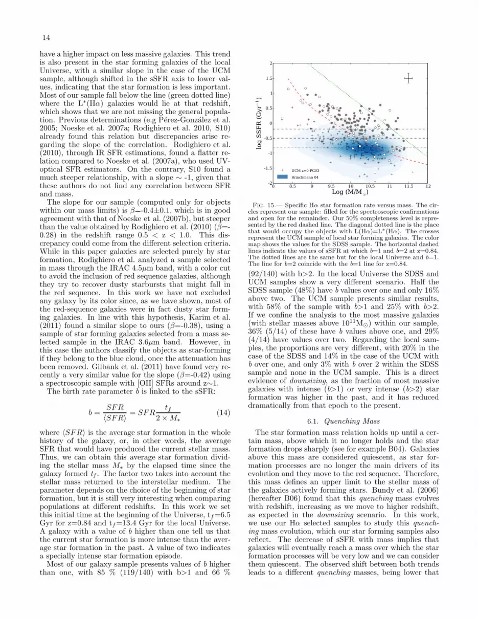
14

have a higher impact on less massive galaxies. This trendis also present in the star forming galaxies of the localUniverse, with a similar slope in the case of the UCMsample, although shifted in the sSFR axis to lower val-ues, indicating that the star formation is less important.Most of our sample fall below the line (green dotted line)where the L∗(Hα) galaxies would lie at that redshift,which shows that we are not missing the general popula-tion. Previous determinations (e.g Perez-Gonzalez et al.2005; Noeske et al. 2007a; Rodighiero et al. 2010, S10)already found this relation but discrepancies arise re-garding the slope of the correlation. Rodighiero et al.(2010), through IR SFR estimations, found a flatter re-lation compared to Noeske et al. (2007a), who used UV-optical SFR estimators. On the contrary, S10 found amuch steeper relationship, with a slope ∼ -1, given thatthese authors do not find any correlation between SFRand mass.The slope for our sample (computed only for objects

within our mass limits) is β=-0.4±0.1, which is in goodagreement with that of Noeske et al. (2007b), but steeperthan the value obtained by Rodighiero et al. (2010) (β=-0.28) in the redshift range 0.5 < z < 1.0. This dis-crepancy could come from the different selection criteria.While in this paper galaxies are selected purely by starformation, Rodighiero et al. analyzed a sample selectedin mass through the IRAC 4.5µm band, with a color cutto avoid the inclusion of red sequence galaxies, althoughthey try to recover dusty starbursts that might fall inthe red sequence. In this work we have not excludedany galaxy by its color since, as we have shown, most ofthe red-sequence galaxies were in fact dusty star form-ing galaxies. In line with this hypothesis, Karim et al.(2011) found a similar slope to ours (β=-0.38), using asample of star forming galaxies selected from a mass se-lected sample in the IRAC 3.6µm band. However, inthis case the authors classify the objects as star-formingif they belong to the blue cloud, once the attenuation hasbeen removed. Gilbank et al. (2011) have found very re-cently a very similar value for the slope (β=-0.42) usinga spectroscopic sample with [OII] SFRs around z∼1.The birth rate parameter b is linked to the sSFR:

b =SFR

〈SFR〉= SFR

tf2×M∗

(14)

where 〈SFR〉 is the average star formation in the wholehistory of the galaxy, or, in other words, the averageSFR that would have produced the current stellar mass.Thus, we can obtain this average star formation divid-ing the stellar mass M∗ by the elapsed time since thegalaxy formed tf . The factor two takes into account thestellar mass returned to the interstellar medium. Theparameter depends on the choice of the beginning of starformation, but it is still very interesting when comparingpopulations at different redshifts. In this work we setthis initial time at the beginning of the Universe, tf=6.5Gyr for z=0.84 and tf=13.4 Gyr for the local Universe.A galaxy with a value of b higher than one tell us thatthe current star formation is more intense than the aver-age star formation in the past. A value of two indicatesa specially intense star formation episode.Most of our galaxy sample presents values of b higher

than one, with 85 % (119/140) with b>1 and 66 %

8 8.5 9 9.5 10 10.5 11 11.5 12

Log (M/M⊙)

-2

-1.5

-1

-0.5

0

0.5

1

1.5

2

log SSFR (Gyr−1)

UCM z=0 PG03

Brinchmann 04

Fig. 15.— Specific Hα star formation rate versus mass. The cir-cles represent our sample: filled for the spectroscopic confirmationsand open for the remainder. Our 50% completeness level is repre-sented by the red dashed line. The diagonal dotted line is the placethat would occupy the objects with L(Hα)=L∗(Hα). The crossesrepresent the UCM sample of local star forming galaxies. The colormap shows the values for the SDSS sample. The horizontal dashedlines indicate the values of sSFR at which b=1 and b=2 at z=0.84.The dotted lines are the same but for the local Universe and b=1.The line for b=2 coincide with the b=1 line for z=0.84.

(92/140) with b>2. In the local Universe the SDSS andUCM samples show a very different scenario. Half theSDSS sample (48%) have b values over one and only 16%above two. The UCM sample presents similar results,with 58% of the sample with b>1 and 25% with b>2.If we confine the analysis to the most massive galaxies(with stellar masses above 1011M⊙) within our sample,36% (5/14) of these have b values above one, and 29%(4/14) have values over two. Regarding the local sam-ples, the proportions are very different, with 20% in thecase of the SDSS and 14% in the case of the UCM withb over one, and only 3% with b over 2 within the SDSSsample and none in the UCM sample. This is a directevidence of downsizing, as the fraction of most massivegalaxies with intense (b>1) or very intense (b>2) starformation was higher in the past, and it has reduceddramatically from that epoch to the present.

6.1. Quenching Mass

The star formation mass relation holds up until a cer-tain mass, above which it no longer holds and the starformation drops sharply (see for example B04). Galaxiesabove this mass are considered quiescent, as star for-mation processes are no longer the main drivers of itsevolution and they move to the red sequence. Therefore,this mass defines an upper limit to the stellar mass ofthe galaxies actively forming stars. Bundy et al. (2006)(hereafter B06) found that this quenching mass evolveswith redshift, increasing as we move to higher redshift,as expected in the downsizing scenario. In this work,we use our Hα selected samples to study this quench-ing mass evolution, which our star forming samples alsoreflect. The decrease of sSFR with mass implies thatgalaxies will eventually reach a mass over which the starformation processes will be very low and we can considerthem quiescent. The observed shift between both trendsleads to a different quenching masses, being lower that

15

8 9 10 11 12 13

Log (M/M⊙)

7

8

9

10

11

12

log td (yr)

UCM z=0 PG03

Fig. 16.— Doubling time td versus stellar mass. The circles rep-resent our sample: filled for the spectroscopic confirmations andopen for the remainder. The 50% completeness level is representedby the red dashed line. The crosses represent the UCM local sam-ple of star forming galaxies. The dashed horizontal line indicatesthe doubling time at which we consider a galaxy at z=0.84 as qui-escent. The dotted horizontal line represents the same but for thelocal Universe. Best linear fits computed for both samples are alsoshown.

at the local Universe.With our data it is possible to estimate an upper limit

for the quenching mass. For the sake of clarity we aregoing to use the doubling time td, which is analogous tothe sSFR and is defined as:

td =M∗

SFR (1 −R)=

1

SSFR (1−R)(15)

where R is the fraction of mass returned to the interstel-lar medium which is generally assumed to be ∼0.5 (Bell2003).The doubling time tells us how long will take for that

galaxy to duplicate its stellar mass if its current star for-mation stays constant. Galaxies with a large doublingtime will evolve slowly whereas galaxies with a smallone will evolve quickly. Doubling times versus mass forour sample and the local UCM sample are shown in fig-ure 16. In order to estimate the quenchingmass we definea galaxy as quiescent if its doubling time is higher thanwhat we define as quenching time: tQ = 3 × tH , wheretH is the Hubble time. To obtain the typical mass whichcorresponds to the quenching time we performed severalsteps. First, we simulated 1000 realizations of our sam-ple, varying randomly the values of SFR and mass withintwice the errors, i.e., each object will have values ran-domly distributed in the intervals [M-2∆M, M+2∆M]and [SFRHα-2∆SFRHα, SFRHα+2∆SFRHα]. Second,we do a linear fit of td versus mass only with the objectswhose simulated mass fall above our mass limit. For eachof these fits we compute the quenching mass as the massat which the doubling time td is equal to the quenchingtime tQ. The final quenching mass MQ is the medianof the whole distribution of quenching masses, with theerror determined by the standard deviation of the dis-tribution. The same process has been followed for theUCM sample.We obtain that MQ=1.0+0.6

−0.4×1012M⊙

0 0.2 0.4 0.6 0.8 1.0 1.2 1.4z

10.0

10.5

11.0

11.5

12.0

12.5

log M

Q

B06. ColorB06. SFR([OII])B06. Morphology

This workThis work (No ext)

Fig. 17.— Evolution of the quenching mass limit MQ. Red cir-cles represent the results obtained in this work for the Hα selectedsamples at z∼0.84 and the local Universe. The orange circles arethe estimated quenching masses when no extinction correction isconsidered. The rest of the points correspond to the B06 work ac-cording to the different criteria employed: black squares for mor-phology, green crosses for [OII]λ3727A SFRs and blue triangles forthe (U-B) color.

(log (MQ/M⊙)=12.0±0.2) for the z∼0.84 sample and

MQ=7.9+1.9−1.5×1010M⊙ (log (MQ/M⊙)=10.9±0.1) for the

local sample. If we consider only the spectroscopicallyconfirmed sample we obtain log (MQ/M⊙)=12.2±0.2,slightly higher although compatible within errors. In thecase of z∼0.84 the quenching mass is outside the rangeof masses detected, given the limit on the detection ofmassive galaxies imposed by sampled volume and theequivalent width limit of the survey, which prevents usfrom selecting objects with lower sSFRs. These massesare upper limits, given that at high stellar massesthe correlation between doubling time and mass willbreak as a consequence of quenching. Galaxies withhigher td than predicted by the correlation will appearas the quenching takes over, possibly lowering theaverage quenching mass, specially in the case of z∼0.84,where no galaxies around MQ have been detected. Inorder to detect these galaxies it would be necessary tosurvey larger volumes. In addition, the simulations (seesection 6) show that we may overestimate the quenchingmass at z∼0.84 by ∼0.1 dex, due to the completenesslimits. However, these simulations also shows that wewould be able to detect quenching masses ∼0.5 dex lower(SFR-M∗ slope 20% lower), with a similar dispersion.Our quenchingmass estimation for the local Universe is

in very good agreement with the stellar mass (∼7×1010

M⊙; scaled from a Kroupa to a Salpeter IMF) abovewhich Kauffmann et al. (2003) found a rapid increase inthe fraction of galaxies with old population in the SDSSlocal sample. This change, detected by a transition fromlower values of Dn(4000) to higher values, is also seen asa change in the slope of the µ∗-M∗ (surface stellar massdensity versus stellar mass) correlation. Our result atz∼0.84 is higher than those estimated by B06 at a simi-lar redshift. In their work, they used three different ap-proaches: morphology, U-B color and SFRs derived from[OII] equivalent width. Through the morphology crite-rion they obtained MQ ∼8×1011M⊙ whereas both color

16

TABLE 1Comparison between total and confirmed samples.

Property Total Sample Confirmed Sample(1) (2) (3)

γ Calzetti et al.(2000) 0.55 0.56〈SFRHα〉 11+22

−7M⊙yr−1 14+23

−9M⊙yr−1

〈SFRFUV /SFRHα〉 0.89 0.87〈SFRIR/SFRHα〉 0.95 0.96log (MQ/M⊙) 12.0±0.2 12.2±0.2

Note. — (1) Measured property (2) Value obtained using thewhole sample (3) Value obtained using the sample confirmedwith optical spectroscopy

and SFR criteria provide lower masses∼1011 M⊙ (see fig-ure 17). We have scaled B06 masses from the ChabrierIMF to the Salpeter IMF used in this work adding 0.25dex. Our result is in good agreement with their morphol-ogy based estimation but it is higher than those based incolor or SFR. B06 attributed this difference to a longertimescale in the processes that transform late types intoearly types. However our value is solely based in starformation and no morphology considerations have beendone. One of the caveats of their SFR and color measure-ments is that extinction was not corrected. Therefore,dusty starbursts would appear redder and with lowerSFRs, as they would be classified as red or non-star form-ing galaxies, which translates in lower quenching masses.If we estimate again MQ for our Hα selected sam-ples, but this time without applying the extinction cor-rection, we obtain lower values: MQ=7.6+1.7

−1.4×1010M⊙

log MQ/M⊙=10.88±0.09) for the z∼0.84 sample and

MQ=1.3+0.2−0.2×1010M⊙ (log MQ/M⊙=10.13±0.05) for

the local sample. The effect of the extinction is veryhigh, and is enough to account for the difference betweenB06 morphology and color/SFR estimations. Our resultis also consistent with the work by Perez-Gonzalez et al.(2008), where they found that at z∼0.8 all the stellarmass has been already assembled for objects more mas-sive than M⋆=1012M⊙ and almost fully assembled forobjects with stellar mass in the range 1011.7-1012M⊙.The quenching masses estimated through this method

rely on the definition of tQ, however, independently ofthis parameter, we find a strong evolution between thelocal Universe and z∼0.84. In the local Universe, galaxieswith mass higher than 1011M⊙ are quiescent and theirevolution is limited to interactions with other galaxiesvia dry mergers (or other processes not involving massivestar formation), whereas at z∼0.84, galaxies with massin the range ∼1011− ∼1012M⊙ are still under strong starformation processes. This is, again, in good agreementwith the downsizing scenario. Despite we do not haveenough data to constrain the MQ evolution with red-shift we find that our results are compatible with theparametrization given by B06, i.e MQ ∝(1+z)4.5. Theadded value is that we have extended the redshift base-line to the local Universe, using samples selected uni-formly.

7. SUMMARY AND CONCLUSIONS

In this work we have analyzed the properties of anHα selected sample of star-forming galaxies at z∼0.84,focusing on the star formation and stellar mass.

We have discarded the AGN contaminants throughtwo criteria: X-ray luminosities and IRAC colors. Wefind seven counterparts in X-ray, though three of thempresent very low fluxes, compatible with being originatedby star formation processes. Thus, we only discard thefour objects with fluxes high enough to have an AGN ori-gin. Using IRAC colors we find another ten objects (oneof them already detected in X-rays) that fulfill the cri-terion to be considered AGN. A total of thirteen objectsare finally discarded.The objects of our sample present a median MB=-

20.5±0.9m, brighter by more than one magnitude thanthe UCM local sample of star forming galaxies. Mostof the galaxies belong to the blue sequence with a smallfraction of objects in the green valley and the red se-quence. Once the extinction corrections are applied allthese red objects except two move to the blue sequence,unveiling their dusty nature.A check on the extinction law reveals that the

Calzetti et al. (2000) extinction law is appropriate forour objects, but with E(B-V)stars=0.55 E(B-V)gas.The Hα SFR, without applying the extinction correc-

tion, presents values in the range 2–10 M⊙. We have alsoestimated SFRs with FUV and IR. In the first case, thenon-extinction corrected FUV underestimates the SFRwith respect to Hα. The opposite case is given for theIR, which overestimates the SFR with respect to Hα.These discrepancies are mainly driven by the extinction.Once we apply the extinction correction to both FUVand Hα estimations, all SFR tracers agree within a fac-tor of three and the highest SFRs reach several hundredssolar masses per year.The scattering between the different tracers are cor-

related with the Hα equivalent width. This can be ex-plained through the different weighted age of the objects(which is related to the EW) and the fact that FUV anIR SFRs are sensitive to a longer time range than Hα,being more affected by older populations.We have estimated stellar masses for our sample, find-

ing that the median value is M⋆=1.4+4.6−1.1 × 1010M⊙, in

good agreement with the result obtained by S10 for asample selected with similar criteria as ours. The typicalmass found by Perez-Gonzalez et al. (2008) for an IRACselected sample at this redshift is ten times higher thanthis value.Our sample shows a trend between SFR and stellar

mass. The slope of this trend is in good agreement withthe value obtained by Noeske et al. (2007a) and is flat-ter than the Elbaz et al. (2007) result. The trend is verysimilar to that of the local Universe, although shifted tohigher values of SFR. This indicates that, for the samestellar mass M∗, star forming galaxies at z∼0.84 are un-der stronger star formation episodes than their local anal-ogous.The sSFR shows a negative correlation with stellar

mass. The star formation in more massive galaxies, al-though with higher SFR, has less impact than in lessmassive ones, due to the large stellar mass alreadyformed. The same trend is observed in the local Uni-verse, though shifted to lower sSFRs. This is in goodagreement with the downsizing scenario, in which mas-sive galaxies are formed earlier than less massive ones.The fraction of massive galaxies (M∗ >1011M⊙) under-

17

going strong star formation processes (b>2), ∼29% atz∼0.84 against <3% at the local Universe, also supportsthis scenario.Finally, we have quantified the downsizing estimating

the quenching mass at z∼0.84 and at the local Universebased on the Hα star formation rate. We find thatMQ=1.0+0.6

−0.4×1012M⊙ (log (MQ/M⊙)=12.0±0.2)

at z∼0.84 and MQ=7.9+1.9−1.5×1010M⊙ (log

(MQ/M⊙)=10.9±0.1) in the local Universe. Theevolution since the local Universe is out of doubt,with an increase in the quenching mass of an order ofmagnitude.

We thank Armando Gil de Paz for helpful discussionsand comments. We acknowledge support from the Span-ish Programa Nacional de Astronomıa y Astrofısica un-der grant AYA2009-10368. Partially funded by the Span-ish MICINN under the Consolider-Ingenio 2010 Programgrant CSD2006- 00070: First Science with the GTC.VV acknowledges support from the AstroMadrid Pro-gram CAM S2009/ESP-1496:“Astrofısica y Desarrollos

Tecnologicos en la Comunidad de Madrid” funded bythe Comunidad de Madrid and the European Union.PGP-G acknowledge support from the Ramon y CajalProgram financed by the Spanish Government and theEuropean Union. This work is based in part on obser-vations made with the Spitzer Space Telescope, whichis operated by the Jet Propulsion Laboratory, Caltechunder NASA contract 1407. GALEX is a NASA SmallExplorer launched in 2003 April. We gratefully acknowl-edge NASAs support for construction, operation, andscientific analysis of the GALEX mission. This researchhas made use of the NASA/IPAC Extragalactic Database(NED) which is operated by the Jet Propulsion Labora-tory, California Institute of Technology, under contractwith the National Aeronautics and Space Administra-tion. Based in part on data collected at Subaru Telescopeand obtained from the SMOKA, which is operated by theAstronomy Data Center, National Astronomical Obser-vatory of Japan. We acknowledge Edward L. Wright forhis world wide web cosmology calculator (Wright 2006),which has been used during the preparation of this paper.

REFERENCES

Adelberger, K. L., Steidel, C. C., Shapley, A. E., Hunt, M. P.,Erb, D. K., Reddy, N. A., & Pettini, M. 2004, ApJ, 607, 226

Alexander, D. M. et al. 2003, AJ, 126, 539Alonso-Herrero, A. et al. 2006, ApJ, 640, 167Barmby, P., Huang, J., Ashby, M. L. N., Eisenhardt, P. R. M.,

Fazio, G. G., Willner, S. P., & Wright, E. L. 2008, ApJS, 177,431

Barro, G. et al. 2009, A&A, 494, 63—. 2011a, ApJS, 193, 13—. 2011b, ApJS, 193, 30Bell, E. F. 2003, ApJ, 586, 794Bouwens, R. J. et al. 2009, ApJ, 705, 936—. 2010, ArXiv e-printsBrinchmann, J., Charlot, S., White, S. D. M., Tremonti, C.,

Kauffmann, G., Heckman, T., & Brinkmann, J. 2004, MNRAS,351, 1151, B04

Bruzual, G., & Charlot, S. 2003, MNRAS, 344, 1000Bundy, K. et al. 2006, ApJ, 651, 120, B06Calzetti, D., Armus, L., Bohlin, R. C., Kinney, A. L., Koornneef,

J., & Storchi-Bergmann, T. 2000, ApJ, 533, 682Calzetti, D. et al. 2007, ApJ, 666, 870—. 2005, ApJ, 633, 871Capak, P. et al. 2004, AJ, 127, 180Caputi, K. I. et al. 2006, ApJ, 637, 727Cardelli, J. A., Clayton, G. C., & Mathis, J. S. 1989, ApJ, 345,

245Cardiel, N., Elbaz, D., Schiavon, R. P., Willmer, C. N. A., Koo,

D. C., Phillips, A. C., & Gallego, J. 2003, ApJ, 584, 76Chabrier, G. 2003, PASP, 115, 763Coil, A. L., Newman, J. A., Kaiser, N., Davis, M., Ma, C.,

Kocevski, D. D., & Koo, D. C. 2004, ApJ, 617, 765Connolly, A. J., Szalay, A. S., Dickinson, M., Subbarao, M. U., &

Brunner, R. J. 1997, ApJ, 486, L11+Cowie, L. L., Songaila, A., & Barger, A. J. 1999, AJ, 118, 603Cowie, L. L., Songaila, A., Hu, E. M., & Cohen, J. G. 1996, AJ,

112, 839da Cunha, E., Charlot, S., & Elbaz, D. 2008, MNRAS, 388, 1595Daddi, E. et al. 2007, ApJ, 670, 156Davis, M. et al. 2007, ApJ, 660, L1Devereux, N., Duric, N., & Scowen, P. A. 1997, AJ, 113, 236Dickinson, M., & GOODS Legacy Team. 2001, in Bulletin of the

American Astronomical Society, Vol. 33, Bulletin of theAmerican Astronomical Society, 820–+

Doherty, M., Bunker, A., Sharp, R., Dalton, G., Parry, I., &Lewis, I. 2006, MNRAS, 370, 331

Donley, J. L., Rieke, G. H., Perez-Gonzalez, P. G., & Barro, G.2008, ApJ, 687, 111

Dutton, A. A., van den Bosch, F. C., & Dekel, A. 2010, MNRAS,405, 1690

Elbaz, D. et al. 2007, A&A, 468, 33Erb, D. K., Steidel, C. C., Shapley, A. E., Pettini, M., Reddy,

N. A., & Adelberger, K. L. 2006, ApJ, 647, 128Faber, S. M. et al. 2007, ApJ, 665, 265Fioc, M., & Rocca-Volmerange, B. 1997, A&A, 326, 950Flores, H., Hammer, F., Elbaz, D., Cesarsky, C. J., Liang, Y. C.,

Fadda, D., & Gruel, N. 2004, A&A, 415, 885Flores, H. et al. 1999, ApJ, 517, 148Garn, T. et al. 2010, MNRAS, 402, 2017Geach, J. E., Smail, I., Best, P. N., Kurk, J., Casali, M., Ivison,

R. J., & Coppin, K. 2008, MNRAS, 388, 1473Gilbank, D. G. et al. 2011, MNRAS, 414, 304Glazebrook, K., Blake, C., Economou, F., Lilly, S., & Colless, M.

1999, MNRAS, 306, 843Hammer, F., Flores, H., Elbaz, D., Zheng, X. Z., Liang, Y. C., &

Cesarsky, C. 2005, A&A, 430, 115Hayes, M., Schaerer, D., & Ostlin, G. 2010, A&A, 509, L5+Hopkins, A. M., & Beacom, J. F. 2006, ApJ, 651, 142Hopkins, A. M., Connolly, A. J., & Szalay, A. S. 2000, AJ, 120,

2843Karim, A. et al. 2011, ApJ, 730, 61Kauffmann, G. et al. 2003, MNRAS, 341, 54Kennicutt, R. C. et al. 2009, ApJ, 703, 1672Kennicutt, Jr., R. C. 1998, ARA&A, 36, 189Kroupa, P. 2001, MNRAS, 322, 231Laird, E. S. et al. 2009, ApJS, 180, 102Le Floc’h, E. et al. 2005, ApJ, 632, 169Lee, J. C. et al. 2009, ArXiv e-printsLeitherer, C., Ferguson, H. C., Heckman, T. M., & Lowenthal,

J. D. 1995, ApJ, 454, L19+Lilly, S. J., Le Fevre, O., Hammer, F., & Crampton, D. 1996,

ApJ, 460, L1+Ly, C., Lee, J. C., Dale, D. A., Momcheva, I., Salim, S.,

Staudaher, S., Moore, C. A., & Finn, R. 2011, ApJ, 726, 109Maraston, C. 2005, MNRAS, 362, 799Martin, D. C. et al. 2005, ApJ, 619, L1—. 2007, ApJS, 173, 342Miyazaki, S., Hamana, T., Ellis, R. S., Kashikawa, N., Massey,

R. J., Taylor, J., & Refregier, A. 2007, ApJ, 669, 714Noeske, K. G. et al. 2007a, ApJ, 660, L47—. 2007b, ApJ, 660, L43Oey, M. S., & Kennicutt, Jr., R. C. 1997, MNRAS, 291, 827Park, S. Q. et al. 2010, ApJ, 717, 1181Pascual, S., Gallego, J., & Zamorano, J. 2007, PASP, 119, 30, P07Perez-Gonzalez, P. G. 2003, PASP, 115, 1353

18

Perez-Gonzalez, P. G., Gil de Paz, A., Zamorano, J., Gallego, J.,Alonso-Herrero, A., & Aragon-Salamanca, A. 2003, MNRAS,338, 525, PG03

Perez-Gonzalez, P. G. et al. 2006, ApJ, 648, 987—. 2005, ApJ, 630, 82—. 2008, ApJ, 675, 234Ranalli, P., Comastri, A., & Setti, G. 2003, A&A, 399, 39Reddy, N. A., & Steidel, C. C. 2009, ApJ, 692, 778Rieke, G. H., Alonso-Herrero, A., Weiner, B. J., Perez-Gonzalez,

P. G., Blaylock, M., Donley, J. L., & Marcillac, D. 2009, ApJ,692, 556

Rodighiero, G. et al. 2010, A&A, 518, L25+Salim, S. et al. 2009, ApJ, 700, 161—. 2007, ApJS, 173, 267Salpeter, E. E. 1955, ApJ, 121, 161Schiminovich, D. et al. 2005, ApJ, 619, L47Sobral, D. et al. 2009, MNRAS, 398, 75Sobral, D., Best, P. N., Smail, I., Geach, J. E., Cirasuolo, M.,

Garn, T., & Dalton, G. B. 2010, MNRAS, 1657, S10Stark, D. P., Ellis, R. S., Bunker, A., Bundy, K., Targett, T.,

Benson, A., & Lacy, M. 2009, ApJ, 697, 1493Steidel, C. C., Adelberger, K. L., Giavalisco, M., Dickinson, M.,

& Pettini, M. 1999, ApJ, 519, 1Steidel, C. C., Giavalisco, M., Pettini, M., Dickinson, M., &

Adelberger, K. L. 1996, ApJ, 462, L17+

Steidel, C. C., Shapley, A. E., Pettini, M., Adelberger, K. L., Erb,D. K., Reddy, N. A., & Hunt, M. P. 2004, ApJ, 604, 534

Stern, D. et al. 2005, ApJ, 631, 163Strateva, I. et al. 2001, AJ, 122, 1861Tresse, L., Maddox, S. J., Le Fevre, O., & Cuby, J.-G. 2002,

MNRAS, 337, 369Villar, V., Gallego, J., Perez-Gonzalez, P. G., Pascual, S., Noeske,

K., Koo, D. C., Barro, G., & Zamorano, J. 2008, ApJ, 677, 169,V08

Willmer, C. N. A. et al. 2006, ApJ, 647, 853Wilson, G., Cowie, L. L., Barger, A. J., & Burke, D. J. 2002, AJ,

124, 1258Wright, E. L. 2006, PASP, 118, 1711Wyder, T. K. et al. 2007, ApJS, 173, 293Yan, L., McCarthy, P. J., Freudling, W., Teplitz, H. I., Malumuth,

E. M., Weymann, R. J., & Malkan, M. A. 1999, ApJ, 519, L47Yoshikawa, T. et al. 2010, ApJ, 718, 112Zamorano, J., Gallego, J., Rego, M., Vitores, A. G., & Alonso, O.

1996, ApJS, 105, 343Zamorano, J., Rego, M., Gallego, J. G., Vitores, A. G.,

Gonzalez-Riestra, R., & Rodriguez-Caderot, G. 1994, ApJS, 95,387

19

18 19 20 21 22 23 24

J mag.

8.0

8.5

9.0

9.5

10.0

10.5

11.0

11.5

12.0

Log (M/M

⊙)

Barro et al. 2011

Fig. 18.— Stellar mass versus J band magnitude. The circles represent our sample: filled for the spectroscopic confirmations and openfor the remainder. The small dots are the objects within our redshift range from the Barro et al. (2011a) mass selected sample. The dashedline is the best linear fit for the mass selected sample.

APPENDIX

COMPLETENESS LEVEL AS A FUNCTION OF STELLAR MASS

The SFR completeness level for our sample depends on the stellar mass, due to the selection process, which isbasically a selection in equivalent width. In V08 we simulated the selection process to determine the completenesslevel versus the line flux, but without considering the dependence on stellar masses, as it was unnecessary. The processconsisted in the introduction of simulated galaxies in the real images to check wether or not they were recovered bythe selection method. Fake galaxies were created with different line and continuum fluxes, sizes and inclinations in thereal images. The outcome was the line flux completeness level.The problem we need to address here is at which SFR, corrected for attenuation, the completeness level is 50% as a

function of stellar mass. The main problem is that we need to relate the stellar mass and extinction to the observables,i.e. the broad-band and narrow-band magnitudes. Intuitively, one may think that exists a correlation between thestellar mass and the broad band magnitude. Indeed, as can be seen in figure 18, there is a correlation between thestellar mass and the J magnitude for our sample. However, it might be affected by selection biases, so we also checkthis relation with another sample. For this double-check we use the mass selected sample from the AEGIS databasepresented in Barro et al. (2011a) and Barro et al. (2011b). If we take all the objects with spectroscopic redshift withinthe limits of our sample we obtain a very similar relation. The best fit to the data gives: M∗=23.36 - 0.636 mJ .With this correlation we can assign a stellar mass for an object given its J band flux. Thus, we can check the fraction

of objects selected for a certain line-flux, defined by their emission in the broad and narrow band filters, and a stellarmass, estimated from the broad band flux. The line flux is transformed to SFR applying the corresponding calibration(equation 1) and applying a mean correction for the nitrogen contribution (I([NII]λ6584)/I(Hα)=0.26). At the endwe have a completeness level for each combination of SFR and stellar mass. From this we can obtain the SFR 50%completeness level as a function of mass.However, this completeness does not take into account the attenuation affecting the SFR measurement. To correct

this effect we can apply the extinction correction to the SFR completeness level:

SFR(M∗)corrected50% =SFR(M∗)uncorrected50% 100.4A(Hα) (A1)

where SFR(M∗)uncorrected50% is the Hα SFR for which we are 50% complete at stellar mass M∗.The question that arises now is which amount of extinction to apply. The immediate solution is to apply the

20

mean(median) extinction correction obtained for the sample. However, it is well known that the amount of extinctiondepends on the total SFR. This fact has been shown for the Sobral et al. (2009) sample by Garn et al. (2010). Inparticular these authors find that A(Hα)= 0.73 + 0.44 logSFR(IR). As we saw in section 5.2.2, we can assume thatthe IR derived SFR is equal to the extinction corrected Hα SFR, and thus we can write:

SFR(M∗)corrected50% =SFR(M∗)uncorrected50% 100.4 (a+b×logSFR(M∗)corrected50%

) (A2)

=SFR(M∗)uncorrected50% 10a′+b′×logSFR(M∗)corrected

50% (A3)

with a=0.73, b=0.44, a′=0.4×a and b′=0.4×b. We can find the value of SFR obtaining:

logSFR(M∗)corrected50% =logSFR(M∗)uncorrected50% + a′

1− b′(A4)

This equation gives us the completeness level at 50% considering that the extinction depends on the total SFR. Thecomputed completeness curve is shown in figure 14.