Embed Size (px)
Citation preview
Norwegian School of EconomicsBergen, Spring 2018
Statistical Arbitrage Trading withImplementation of Machine Learning
An empirical analysis of pairs trading on the Norwegian stock market
Hakon Andersen & Hakon Tronvoll
Supervisor: Tore Leite
Master Thesis in Financial Economics
Norwegian School of Economics
This thesis was written as a part of the Master of Science in Economics and BusinessAdministration at NHH. Please note that neither the institution nor the examiners areresponsible - through the approval of this thesis - for the theories and methods used, or
results and conclusions drawn in this work.

Abstract
The main objective of this thesis is to analyze whether there are arbitrage opportunities on
the Norwegian stock market. Moreover, this thesis examines statistical arbitrage through coin-
tegration pairs trading. We embed an analytic framework of an algorithmic trading model
which includes principal component analysis and density-based clustering in order to extract
and cluster common underlying risk factors of stock returns. From the results obtained we
statistically prove that pairs trading on the Oslo Stock Exchange Benchmark Index does not
provide excess return nor favorable Sharpe ratio. Predictions from our trading model are also
compared with an unrestricted model to determine appropriate stock filtering tools, where we
find that unsupervised machine learning techniques have properties which are beneficial for
pairs trading.

Acknowledgements
We would like to direct our appreciation towards our supervisor, Prof. Tore Leite, for valuable
input and guidance throughout this process. Also, we would like show gratitude towards Bard
Tronvoll for his reflections and insights.
Last, we would like to thank all our friends at NHH who have been supportive throughout the
years.
Contents
Abstract ii
Acknowledgements ii
1 Introduction 1
1.1 Background . . . . . . . . . . . . . . . . . . . . . . . . . . . . . . . . . . . . . . 1
1.2 The Aim of this Thesis . . . . . . . . . . . . . . . . . . . . . . . . . . . . . . . . 2
1.3 Structure of Thesis . . . . . . . . . . . . . . . . . . . . . . . . . . . . . . . . . . 3
2 Theoretical Frameworks 4
2.1 The Efficient-Market Hypothesis . . . . . . . . . . . . . . . . . . . . . . . . . . . 4
2.1.1 Pure Arbitrage vs. Statistical Arbitrage . . . . . . . . . . . . . . . . . . 7
2.2 The Arbitrage Pricing Theory . . . . . . . . . . . . . . . . . . . . . . . . . . . . 10
2.3 Pairs Trading . . . . . . . . . . . . . . . . . . . . . . . . . . . . . . . . . . . . . 12
2.3.1 Empirical Evidence of Pairs Trading . . . . . . . . . . . . . . . . . . . . 14
3 Research Design and Methodology 16
3.1 Overview of the Research Design . . . . . . . . . . . . . . . . . . . . . . . . . . 16
3.2 Stage 1: Data Management . . . . . . . . . . . . . . . . . . . . . . . . . . . . . 18
iv
CONTENTS v
3.3 Stage 2: Stock Filtering . . . . . . . . . . . . . . . . . . . . . . . . . . . . . . . 19
3.3.1 Machine Learning . . . . . . . . . . . . . . . . . . . . . . . . . . . . . . . 19
3.3.2 Principal Component Analysis . . . . . . . . . . . . . . . . . . . . . . . . 20
3.3.3 Density-Based Spatial Clustering of Applications with Noise . . . . . . . 24
3.3.4 t-Distributed Stochastic Neighbor Embedding . . . . . . . . . . . . . . . 25
3.4 Stage 3: Identifying Mean-Reversion . . . . . . . . . . . . . . . . . . . . . . . . 27
3.4.1 The Cointegration Approach . . . . . . . . . . . . . . . . . . . . . . . . . 27
3.5 Stage 4: Trading Setup and Execution . . . . . . . . . . . . . . . . . . . . . . . 30
3.5.1 Trading Signals and Execution . . . . . . . . . . . . . . . . . . . . . . . . 30
3.5.2 Training and Testing Periods . . . . . . . . . . . . . . . . . . . . . . . . 31
3.5.3 Transaction costs . . . . . . . . . . . . . . . . . . . . . . . . . . . . . . . 33
3.5.4 Performance Measures and Hypothesis Testing . . . . . . . . . . . . . . . 34
3.6 Research Design Review . . . . . . . . . . . . . . . . . . . . . . . . . . . . . . . 36
4 Results 37
4.1 Determining the Number of Principal Components . . . . . . . . . . . . . . . . 37
4.2 Cluster Discovering . . . . . . . . . . . . . . . . . . . . . . . . . . . . . . . . . . 39
4.3 Summary of the Results . . . . . . . . . . . . . . . . . . . . . . . . . . . . . . . 42
4.3.1 Summary of the Results Without Transaction Costs . . . . . . . . . . . . 42
4.3.2 Summary of the Results with Transaction Costs . . . . . . . . . . . . . . 46
4.3.3 Comparing the Strategy with an Unrestricted Model . . . . . . . . . . . 48
4.4 Empirical Summary . . . . . . . . . . . . . . . . . . . . . . . . . . . . . . . . . . 49
5 Discussion 50
5.1 The Efficient-Market Hypothesis . . . . . . . . . . . . . . . . . . . . . . . . . . . 50
5.2 The Arbitrage Pricing Theory . . . . . . . . . . . . . . . . . . . . . . . . . . . . 52
5.3 Pairs Trading . . . . . . . . . . . . . . . . . . . . . . . . . . . . . . . . . . . . . 53
5.4 Discussion Summary . . . . . . . . . . . . . . . . . . . . . . . . . . . . . . . . . 55
6 Conclusion 56
6.1 Summary . . . . . . . . . . . . . . . . . . . . . . . . . . . . . . . . . . . . . . . 56
6.2 Limitations and Future Work . . . . . . . . . . . . . . . . . . . . . . . . . . . . 57
References 59
7 Appendices 65
7.1 The different forms of market efficiency . . . . . . . . . . . . . . . . . . . . . . . 65
7.2 Returns, Volatility and Sharp ratio . . . . . . . . . . . . . . . . . . . . . . . . . 66
7.2.1 Return and volatility calculation . . . . . . . . . . . . . . . . . . . . . . 66
7.2.2 Return, Volatility and Sharpe Ratio for each stock pair . . . . . . . . . . 66
7.3 Clusters formed . . . . . . . . . . . . . . . . . . . . . . . . . . . . . . . . . . . . 71
7.4 Python Code . . . . . . . . . . . . . . . . . . . . . . . . . . . . . . . . . . . . . 73
7.4.1 Stage 1: Data Management . . . . . . . . . . . . . . . . . . . . . . . . . 73
7.4.2 Stage 2: Stock Filtering . . . . . . . . . . . . . . . . . . . . . . . . . . . 74
7.4.3 Stage 3: Identifying Mean-Reversion . . . . . . . . . . . . . . . . . . . . 76
7.4.4 Stage 4: Trading Setup and Execution . . . . . . . . . . . . . . . . . . . 82
7.5 First principal component vs. OSEBX . . . . . . . . . . . . . . . . . . . . . . . 93
vi

List of Tables
3.1 Total transaction costs per trade for all stock pairs expressed in BPS . . . . . . 33
3.2 Review of the Research Design . . . . . . . . . . . . . . . . . . . . . . . . . . . . 36
4.1 Stocks in clusters from training period 1 . . . . . . . . . . . . . . . . . . . . . . 41
4.2 Summary statistics of portfolio without transaction costs . . . . . . . . . . . . . 42
4.3 One-tailed t-test on portfolio alpha without transaction costs . . . . . . . . . . . 44
4.4 Two-tailed t-test on portfolio beta . . . . . . . . . . . . . . . . . . . . . . . . . . 45
4.5 Summary statistics of portfolio with transaction costs . . . . . . . . . . . . . . . 46
4.6 One-tailed t-test on portfolio alpha with transaction costs . . . . . . . . . . . . . 47
4.7 Summary statistics of Unrestricted and Restricted model without transaction costs 48
7.1 Different forms of market efficiency . . . . . . . . . . . . . . . . . . . . . . . . . 65
7.2 Equal weighted portfolio period 1 . . . . . . . . . . . . . . . . . . . . . . . . . . 66
7.3 Equal weighted portfolio period 2 . . . . . . . . . . . . . . . . . . . . . . . . . . 67
7.4 Equal weighted portfolio period 3 . . . . . . . . . . . . . . . . . . . . . . . . . . 67
7.5 Equal weighted portfolio period 4 . . . . . . . . . . . . . . . . . . . . . . . . . . 68
7.6 Equal weighted portfolio period 5 . . . . . . . . . . . . . . . . . . . . . . . . . . 68
7.7 Equal weighted portfolio period 6 . . . . . . . . . . . . . . . . . . . . . . . . . . 69
vii

7.8 Equal weighted portfolio period 7 . . . . . . . . . . . . . . . . . . . . . . . . . . 69
7.9 Equal weighted portfolio period 8 . . . . . . . . . . . . . . . . . . . . . . . . . . 70
viii

List of Figures
2.1 Dependency structure of two assets with the same underlying factors . . . . . . 11
3.1 Overview of research design . . . . . . . . . . . . . . . . . . . . . . . . . . . . . 16
3.2 Overview of training and testing periods . . . . . . . . . . . . . . . . . . . . . . 32
4.1 Determining the number of principle components . . . . . . . . . . . . . . . . . 38
4.2 Clusters formed in all training periods . . . . . . . . . . . . . . . . . . . . . . . 40
4.3 Visualization of clusters formed from training period 1 . . . . . . . . . . . . . . 41
4.4 Value development for pairs trading strategy and benchmark index . . . . . . . 43
4.5 Daily return distribution over the sample period . . . . . . . . . . . . . . . . . . 45
4.6 Strategy with and without transaction costs compared to benchmark . . . . . . 47
4.7 Restricted and Unrestricted model comparison . . . . . . . . . . . . . . . . . . . 49
7.1 Clusters formed in all training periods . . . . . . . . . . . . . . . . . . . . . . . 71
7.2 Linear relationship between filtered stocks . . . . . . . . . . . . . . . . . . . . . 78
7.3 MHG-WWIB stock pair . . . . . . . . . . . . . . . . . . . . . . . . . . . . . . . 79
7.4 Engle-Granger first step . . . . . . . . . . . . . . . . . . . . . . . . . . . . . . . 81
7.5 Trading Positions . . . . . . . . . . . . . . . . . . . . . . . . . . . . . . . . . . . 85
7.6 MHG-WWIB Pair Return . . . . . . . . . . . . . . . . . . . . . . . . . . . . . . 86
ix

7.7 Pairs cumulative returns from period 1 . . . . . . . . . . . . . . . . . . . . . . . 89
7.8 Portfolio - period 1 . . . . . . . . . . . . . . . . . . . . . . . . . . . . . . . . . . 92
7.9 First principal components vs. OSEBX . . . . . . . . . . . . . . . . . . . . . . . 93
x

Chapter 1
Introduction
1.1 Background
Has someone ever told you that there is no such thing as a free lunch? This is a knowledgeable
proverb expressing the idea that it is impossible to get something for nothing. In mathematical
finance, the term is used to describe the principle of no-arbitrage, which states that it is not
possible to make excess profit without taking risk and without a net investment of capital
(Poitrast, 2010). The recent development of modern technological novelties has aided the idea
of no-arbitrage because it has disrupted the economic infrastructure and the working conditions
in the financial markets. Two important interrelated technological shifts have been crucial to
this progress. First, advanced computer technology has enabled investors to automate their
trading through sophisticated trading algorithms. Second, stock exchanges have structured
themselves in a completely computerized way which makes access to capital easier than ever
(Avolio et al., 2002). These are all contributions which have led to increased market efficiency
and transparency and, one can wonder if the progress has come so far that it has created a
perfectly efficient market where the idea of no-arbitrage is, in fact, a striking reality?
Although this may be the new outlook, market inefficiencies may arise every now and then.
The problem is just to identify such rare situations before they disappear. On these premises,
financial institutions are now allocating huge resources to develop trading algorithms which
1

can locate such scarce market inefficiencies. As a consequence, learning to understand these
algorithms can give you the skills to leverage market information in a way that disproves the
notion of no-arbitrage. Therefore, by understanding and analyzing the intersection between
trading algorithms and mathematical finance, might there be a free lunch after all?.
1.2 The Aim of this Thesis
In the attempt to investigate if there is a ”free lunch” in the market, we want to identify
stocks which have deviated from its relatively fundamental value. Moreover, we seek to develop
an algorithmic trading model capitalizing on the notion of statistical arbitrage. This will be
executed through the trading strategy known as pairs trading.
Pairs trading is a relative value statistical arbitrage strategy that takes a position in the spread
between two stocks which prices have historically moved in tandem (Gatev et al., 2006). More
specifically, one enters a long position in one stock and a short position in the other. Positions
are executed simultaneously. The spread between the two stocks forms a stationary process,
where trading signals are based on deviations from the long-term equilibrium spread. If the
spread deviates from its historical equilibrium, we act and capitalize on the temporary incon-
sistency in the belief it will revert back in the nearest future. Since stock prices are assumed to
follow a stochastic process, the strategy only needs to account for the relative price relationship
between the stocks. This implies that the long position is entered in the understanding that
the stock is relatively undervalued compared to the other and, must, therefore, be balanced by
a short position (Harlacher, 2016). Hence, pairs trading gives no indications that stocks are
mispriced in absolute terms because it bets on the relative relationship between two stocks to
be mean-reverting (Harlacher, 2016).
In the last decades, various scholars have demonstrated unique methods of constructing a pairs
trading strategy with declining profitability in recent time mainly due to improved technology.
Nevertheless, the vast majority of the documented studies have been carried out in the US equity
markets, thus leaving us with a scarce amount of research outside the region. This academic
2
ambiguity has further triggered our interest to undertake a study aiming to acquire knowledge
on the profitability of such a strategy in Norway. To scrutinize the search of statistical arbitrage,
we implement techniques of unsupervised machine learning to effectively filter stocks. The Oslo
Stock Exchange Benchmark Index is the considered stock universe and has been used to measure
the performance from the period of January 2013 to December 2017. Thus, to see if algorithmic
pairs trading is profitable in Norway, we impose the following research question:
Can algorithmic pairs trading with machine learning generate excess return?
In the pursuit of the research question, we have constructed our research design as a four stage
process. The interrelated stages are i) data management, ii) stock filtering, iii) identifying
mean-reversion, and iv) trading setup and execution. Below is an outline of the study of these
stages.
The first stage of the research design encompasses the process of data sampling and manage-
ment, where we implement stock return and fundamental ratios. For the stock filtering process,
we embed three different methods of unsupervised machine learning techniques to find natural
clusters of common underlying risk factors. In the third stage, clustered stocks are tested for
cointegration as a mean to identify mean-reversion. For the last, we instrument trading signals
and thresholds for buy and sell.
1.3 Structure of Thesis
The thesis is organized as follows: Chapter 2 outlines the theoretical frameworks for this thesis.
In Chapter 3, we present our research design and the methodology used. In Chapter 4, we
present the empirical results obtained. From there, Chapter 5 discusses the results in light of
the theoretical frameworks. Last, in Chapter 6, we conclude our findings.
3
Chapter 2
Theoretical Frameworks
2.1 The Efficient-Market Hypothesis
The ”free lunch” principle is supported by the Efficient-Market Hypothesis (EMH), which
states that transactions in an efficient market are at its correct value because all information
is reflected in the price (Fama, 1970). The theory thus provides a theoretical indication of the
outcome of our research question because one cannot exploit mispriced stocks when there are
none. Moreover, Jensen (1978) contributes to the definition by defining market efficiency as,
”A market is said to be efficient if it is impossible to make a profit by trading on a set of
information, Ωt”
From the definition, as outlined by Jensen (1978) and Fama (1970), market efficiency relies on,
i) the information set adapted, Ωt, and ii) the ability to exploit this information. The former
criteria postulate that market efficiency exists in three various forms on the basis of the infor-
mation set, namely the weak, semi-strong and strong. If Ωt only contains past information, the
EMH is at its weak form (Timmermann and Granger, 2004). The semi-strong form indicates
that the information set includes all past and present public information. Such information
includes fundamental data such as product line, quality of management, balance sheet compo-
sition and earning forecasts (Bodie et al., 2014). Last, if Ωt contains both public and private
4
information, the EMH is in its strong form (Malkiel, 2005). For a more detailed description of
all forms of market efficiency, see Appendix 7.1.
For the second criteria, the EMH implies the idea of no-arbitrage. A situation where an
investor is not able to obtain excess return from the information set because it reflects all
relevant information. Moreover, Fama (1970) elevates the concept as,
E(P j,t+1 | Ωt) = [1 + E(Rj,t+1 | Ωt)]Pjt (2.1)
where E is the expected value, Pjt is the price of stock j at time t. Rj,t+1 is the stock return
defined by (Pj,t+1−Pjt)/(Pjt). The tildes indicates that Pj,t+1 and Rj,t+1 are random variables
in the given time, conditional on the information set Ωt. Equation (2.1) simply states that
the expected stock price at time t + 1 is a function of the expected return and the price at
time t. Fama (1970) then argues that this has a major empirical impact because it rules out
any possibility to expect excess returns. Because of this, the expected value should, therefore,
reflect the actual value and we can define,
Zj,t+1 = Rj,t+1 − E(Rj,t+1 | Ωt) (2.2)
then,
E(Zj,t+1 | Ωt) = 0 (2.3)
where equation (2.3) is the excess market return of the stock at t + 1. Moreover, it is the
difference between the observed return and the expected return with the property that the
excess value is zero. Fama (1970) describes this condition as a fair game, an uncertain situation
in which the differences between expected and actual outcomes show no systematic relations
(Law and Smullen, 2008). If we describe α(Ωt) = [α1(Ωt)+α2(Ωt)+ ...+αn(Ωt)] as the amount
of capital invested in each of the n available stocks based on the information Ωt, Fama (1970)
5
now argues that the excess market value at time t+ 1 is,
E(Vj,t+1) =n∑j=1
αj(Ωt)E(Zj,t+1 | Ωt) = 0 (2.4)
where the total excess market value is a fair game with a value of zero. This is because
rational investors are able to gather relevant information and thus, investors do not have any
comparative advantage. Hence, the expected value thus equals the observed value, meaning
that there is no such thing as a free lunch. As aforementioned, Fama (1970) outlines that
stock prices fully reflect all information. Some information is expected and some unexpected.
The unexpected portion of this information arrives randomly, and the stock price is adjusted
according to this new information. Fama (1970) outlines this as a random walk. He describes
successive price changes to be independent and identically distributed such that,
Pjt = Pj,t−1 + µt (2.5)
where µt is a white noise process with a mean of zero and variance σ2. This means, that under
the rubric of the EMH, Pjt is said to be marginal because the best forecast of all values Pj,t+1
is the current price Pt (Pesaran, 2010). The random walk model then becomes,
f(Rj,t+1 | Ωt) = f(Rj,t+1) (2.6)
with f indicating the probability density function. The model of the random walk is an impor-
tant concept for our research because it states that we cannot determine the precise return in
advance. Over the long run, stock returns are consistent with what we expect, given their level
of risk. However, in the short-run, fluctuations can affect the long-run prospect (Fama, 1970).
Nevertheless, there is empirical evidence that sheds doubts about the efficiency of markets and
the unpredictability of stock prices. Moreover, various scholars ample evidence of excess return
predictably caused by a long-term equilibrium between the relative prices of two financial time
series. Any deviations from this relative equilibrium state are coming from a temporary shock
6
or reaction from the market and thus, creating arbitrage opportunities (Bogomolov, 2013). In
the 1980’s, Poterba and Summers (1988) documented this contrarian-strategy, which indicates
that underperforming stocks (losers) yielded substantially better returns than the overperform-
ers (winners). This was an indication of mean-reversion, an idea that the stocks would revert
back to its equilibrium form after an event. Moreover, the authors examined 17 different foreign
equity markets, analyzing the statistical evidence bearing on whether transitory components
justifies a large portion of the variance in common stock returns. They concluded that the
explanation of the mean-reverting behavior was due to time-varying returns and speculative
bubbles which caused stock prices to deviate from its fundamental values (Poterba and Sum-
mers, 1988).
Furthermore, mean-reversion can also be discovered in light of investment behavior. De Bondt
and Thaler (1985) conducted a market research on investment behavior, analyzing the links
between mean-reversion and overreaction in the market. Their hypothesis proclaimed that
individuals tend to put more effort on news pointing in the same direction, resulting in the
systematical mispricing of stock prices. This irrational behavior, as pointed out by De Bondt
and Thaler (1985), is ameliorated by successive price movements in opposite course to its correct
market value. Thus, acting on underpriced losers and overpriced winners yielded cumulative
abnormal returns over the investment period. Thus, discovering a substantial weak form of
market inefficiencies.
2.1.1 Pure Arbitrage vs. Statistical Arbitrage
We have now outlined the concept of the Efficient-Market Hypothesis where the idea of no-
arbitrage is a central element. We, therefore, deliberate in greater detail the concept of arbitrage
and its distinction from statistical arbitrage.
The concept of arbitrage, as outlined by Do and Faff (2010), is a strategic process that capitalizes
on inconsistencies in assets prices without any form of risk or net investment. The notion refers
to buying an asset in one market and simultaneously selling it in another at a higher price,
thus profiting from the temporary differences in the two prices. In more detail, Bjork (1998)
7
defines a pure arbitrage possibility as a self-financing portfolio h where the value process has
a deterministic value at t=0 and a positive stochastic value Vt at time t ≥ 0. If we let hi(t)
denote the number of shares in the portfolio, and Si(t) the price of a stock which trades in
continuous time, than the value of the portfolio will be,
Vt =n∑i=1
hi(t)Si(t) (2.7)
Then the portfolio∑n
i=1 hi(t) is said to be self-financing if,
dVt =n∑i=1
hi(t)dSi(t) (2.8)
The derived equation indicates that when new prices S(t) are manifested at time t, one re-
balances the portfolio (Bjork, 1998). The re-balancing consists of purchasing new assets through
the sale of old assets which already exists in the portfolio. Moreover, the self-financing portfolio
can consist of long and short positions in several risky assets which results in a zero initial cost.
This means that the portfolio is self-financing because there is no exogenous infusion or removal
of money (Lindstrom et al., 2015). On the premise of self-financing strategies, Bjork (1998)
defines arbitrage as a portfolio h with a cumulative discounted value such that,
V h0 = 0 (2.9)
P (V hT ≥ 0) = 1 (2.10)
P (V hT > 0) > 0 (2.11)
where equation (2.9) states that the portfolio is self-financed and has a zero initial cost. The
second property (2.10) states that there is a 100% probability of a portfolio value of zero or
greater. Furthermore, (2.11) expresses that there is always a probability of obtaining a dis-
counted cumulative terminal value of greater than zero. This means that arbitrage is considered
a risk-free profit after transaction costs (Bjork, 1998).
8
Nevertheless, in the financial markets, an investor looking for an arbitrage opportunity typically
engages in a trade that involves some degree of risk. In the specific case where these risks are
statistically assessed through the use of mathematical models, it is appropriate to use the term
statistical arbitrage (Lazzarino et al., 2018). Following the definition of Hogan et al. (2004), a
statistical arbitrage is where the overall expected payoff is positive, but there is a probability of
a negative outcome. Only when the time aspect approaches infinity and we repeat the process
continuously, the negative payoff will converge towards zero. Given a stochastic process of the
trading value on a probability space Ω, F, P, Hogan et al. (2004) outlines four conditions for
a statistical arbitrage portfolio,
V h0 = 0 (2.12)
limt→∞
E[V ht ] > 0 (2.13)
limt→∞
P (V ht ) < 0 = 0 (2.14)
limt→∞
V ar[V ht ]
t= 0 if P (V h
t < 0) > 0, ∀t <∞ (2.15)
where the first property inherent in a zero initial cost strategy i.e it is self-financing (2.12).
Furthermore the strategy, in the limit, has a positive expected discounted cumulative cash flow
(2.13) and, a probability of a loss approaching zero (2.14). Last, the average variance (over
time) is converging to zero if the probability of a loss does not become zero in finite time (2.15).
The last equation is only employed if there is a positive probability of losing money, because
if P (V ht < 0) = 0 , ∀t ≥ T with T < ∞, it describes the basic arbitrage as outlined by Bjork
(1998). Hence, a statistical arbitrage will accumulative riskless profit in the limit.
9
2.2 The Arbitrage Pricing Theory
In the second theoretical point of departure, we will outline the Arbitrage Pricing Theory (APT)
as a mean to discover the ”free lunch”. As first outlined by Ross (1975), the APT is based on
the idea that stock returns can be predicted using a linear model of multiple systematic risk
factors. Ross (1975) describes these factors as economic risk factors such as business cycles,
interest rate fluctuations, inflation rules etc. According to Ross (1975), the exposure of these
factors will affect a stocks risk and hence, its expected return. While pure arbitrage imposes
restrictions on prices observed at a specific point in time, the APT seeks to explain expected
returns at different points in time (Poitrast, 2010). Because of this, any deviation from the
theoretical optimum can be seen as a mispriced stock. As described by Vidyamurthy (2004)
and Harlacher (2016), the theory uncover the heart of pairs trading because stocks with the
same risk exposure will provide the same long-run expected return and, therefore, the APT
may serve as a catalyst to identify arbitrary opportunities.
This line of thinking will be the basis of our statistical arbitrage strategy. If we are able to
identify stocks with similar risk profile, any deviation from the APT expectation will be an
opportunity to capitalize on relative mispriced stocks. Moreover, Harlacher (2016) outlines the
relationship as presented in Figure 2.1, where the co-movement between two stocks only exists
due to their common relation to underlying factors.
In greater detail, the APT structure the expected return of a stock in the following way,
ri = βo +k∑j=1
βi,jFj + ui (2.16)
where Fj can be seen as a factor, and βi,j as the risk exposure of that factor. The βo together
with ui are interpreted as the idiosyncratic part of the observed return. In addition to this
linear dependence structure as outlined by Harlacher (2016) and Ross (1975), there are other
assumptions pertaining to this model:
10
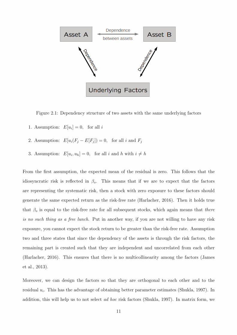
Figure 2.1: Dependency structure of two assets with the same underlying factors
1. Assumption: E[ui] = 0, for all i
2. Assumption: E[ui(Fj − E[Fj]) = 0, for all i and Fj
3. Assumption: E[ui, uh] = 0, for all i and h with i 6= h
From the first assumption, the expected mean of the residual is zero. This follows that the
idiosyncratic risk is reflected in βo. This means that if we are to expect that the factors
are representing the systematic risk, then a stock with zero exposure to these factors should
generate the same expected return as the risk-free rate (Harlacher, 2016). Then it holds true
that βo is equal to the risk-free rate for all subsequent stocks, which again means that there
is no such thing as a free lunch. Put in another way, if you are not willing to have any risk
exposure, you cannot expect the stock return to be greater than the risk-free rate. Assumption
two and three states that since the dependency of the assets is through the risk factors, the
remaining part is created such that they are independent and uncorrelated from each other
(Harlacher, 2016). This ensures that there is no multicollinearity among the factors (James
et al., 2013).
Moreover, we can design the factors so that they are orthogonal to each other and to the
residual ui. This has the advantage of obtaining better parameter estimates (Shukla, 1997). In
addition, this will help us to not select ad hoc risk factors (Shukla, 1997). In matrix form, we
11
can rewrite (2.16) as,
ri = βo + βTi Fj + ui (2.17)
where ui is a vector of random variables and Fj is a (k + 1) vector of random factors. If
we normalize the variables, we get E[Fj] = 0 and E[ui] = 0, then the factor model implies
E[ri] = βo. If this relationship truly exists with the underlying assumptions, Harlacher (2016)
outlines the variance and the covariance of the stocks as,
V ar(ri) = βTi V βi + σ2i (2.18)
Cov(ri, rh) = βTi V βh (2.19)
with σ2i = E[u2
i ], and V being a (k+ 1)× (k+ 1) matrix with the covariance factor changes. As
aforementioned, we will in this thesis utilize the APT to extract the underlying risk factors to
better seek arbitrage opportunities. Moreover, we will follow the line of thinking of Chamberlain
and Rothschild (1983) by using the principal component analysis to estimate and extract the
common underlying factors by composing the eigenvectors. This will be the initial foundation
when forming our research design for conducting a pairs trading strategy.
2.3 Pairs Trading
In the world of finance, pairs trading is considered the origin of statistical arbitrage (Avellaneda
and Lee, 2008). It is a statistical arbitrage strategy which matches a long position with a short
position of two stocks with relatively similar historical price movements. Even though there are
several approaches to pairs trading, this thesis will analyze pairs trading through the concept
of cointegration, as presented by Vidyamurthy (2004). Jaeger (2016) argues that cointegration
between two stocks implies that there is a weak form of market efficiency because it opens for
arbitrary situations based on historical information. This statistical relationship is, therefore,
necessary to explain why there can be a presence of pairs trading (Jaeger, 2016).
12
If Yt and Xt denotes the corresponding prices of two stocks with the same stochastic process,
Avellaneda and Lee (2008) models the system on differentiated form as,
dYtYt
= dαt + βdXt
Xt
+ dSt (2.20)
Where St is a stationary process and the cointegrated spread. This means that the spread
between the two stocks do not drift apart too much and in the ideal case, the spread has a
constant mean over time. If the spread deviates from its historical mean, we act and capitalize
on the temporary inconsistency. During trading, limits are set on the top and bottom of the
spread. If it ever goes below or above a particular normalized spread score, one will go long or
short in the spread. In more detail, by entering a long position in the spread, the investor buys
one unit of stock Yt and short β units of stock Xt, which implies that the spread St is below
the equilibrium average (Avellaneda and Lee, 2008). Consequently, an opposite position will
be entered if one goes short in the spread. This implies that one buy the relatively undervalued
stock and sell the relatively overvalued stock in such portion that the total position is non-
sensitive to overall market movements i.e the portfolio beta becomes zero (Harlacher, 2016).
Once a trading signal like this occurs, a reversion to the historical mean is expected. The
position will be closed when convergence is close to the mean (Kakushadze, 2014).
In light of the efficient-market hypothesis, if a cointegrated relationship between two stocks is
identified we can expect two outcomes: i) the relationship may cease to exists and the weak
form of market-efficiency holds true, which will result in a profit loss. This could be a result of
news or shocks related to any of the stocks, and the recovery of such an event might last longer
than the estimated trading period, or utmost, never at all. ii) The cointegrated relationship is,
in fact, true and we will trade in the spread levels (Jaeger, 2016), which will result in a rejection
of the weak-form of market efficiency.
In theory, pairs trading cannot be justified under the efficient market hypothesis. This needs
to be violated through a mean-reverting behavior of stock prices, which ensures a relative long-
term equilibrium between two stocks (Jaeger, 2016). The question is then if there are such
13
violations of the efficiency of markets, and what have scholars and investors historically done?
2.3.1 Empirical Evidence of Pairs Trading
It was not until the work of Gatev et al. (1999) that the first empirical strategy of mean-reversion
was used on pairs trading. In the article, they employed a method named the distance approach,
a technique engaging in deviations between normalized prices. In their study, they back-tested
a pairs trading strategy on U.S equities, in the period of 1967 to 1997. Their strategy yielded
excess return of 11%, robust for any transaction costs. Notwithstanding, the article of Gatev
et al. (1999) extended the notion of its ancestors in that it deliberated the importance of mean
reversion for generating pairs trading profits. The same article was reproduced in 2006 where
they expanded the data period by five years, still with positive results.
Succeeding the study of Gatev et al. (2006), Do and Faff (2010) replicated the study by ex-
panding the sample period by seven years. With the growing popularity of pairs trading and
the technological advancement in the financial markets, they wanted to analyze whether the
strategy could still produce excess return. Do and Faff (2010) argued that the increased com-
petition among arbitrageurs would result in situations where even the smallest opportunity
would be exploited. In addition, the arbitrageurs would face risks such as fundamental risk and
synchronization risk which all work to prevent arbitrage. In their study, they revealed declining
profits of pairs trading over the sample period. This was because of fewer convergence prop-
erties, higher arbitrage risk, and increased market efficiency. However, consistent with Gatev
et al. (2006), Do and Faff (2010) claimed that pairs trading worked particularly well in time
of financial crisis. This aspect is further investigated by Acharya and Pedersen (2005) which
found that the profitability of pairs trading is negatively correlated with market liquidity.
In recent years, the advent of computer power and statistical methods has contributed to more
advanced methods to the field of pairs trading. Some of these are through various machine
learning techniques. The most cited article to include a principal component analysis (PCA)
in pairs trading was conducted by Avellaneda and Lee (2008). In their training period, they
used PCA as a mean to decompose and extract risk components, as a way to sort out the
14

idiosyncratic noise. The strategy yielded excess returns but received critique since the authors
experimented with different threshold for entry and exit signals. PCA has also been used for
portfolio optimization, as described in Tan (2012) where he gained positive results in terms of
portfolio efficiency.
15

Chapter 3
Research Design and Methodology
This chapter introduces the main data and methodology used in our research design. The first
sub-chapter gives a brief explanation of the different stages of our research design. Further
on, we present each stage process with its respective theoretical and methodical concepts. All
methodological work is conducted in the open source program Python and the python code for
each stage are presented in Appendix 7.4.
3.1 Overview of the Research Design
For our research design, our main goal is to create an algorithm suitable for an efficient pairs
trading strategy. To make our research design more transparent and easy to follow, we have
designed it as an interrelated four stage process. The figure below describes the process of the
different stages.
Stage 1-3 are stages which seeks to find valid and suitable stock pairs. Stage 4 isthe last stage process where we enter trading positions.
Figure 3.1: Overview of research design
16

Stage one encompasses the process of data sampling and management. The data sample consists
of daily returns and fundamental ratios of all companies at The Oslo Stock Exchange Benchmark
Index. In this way, we can analyze price pattern and movements through the dimensions of
price data and fundamental ratios.
In the second stage, we have structured our data through different unsupervised machine learn-
ing techniques. This is done so we can extract and cluster common underlying risk factors of
stock returns. The first unsupervised method is a principal component analysis, a tool used
for dimensionality reduction and factor analysis. We then apply a density-based clustering
technique, a method for discovering unknown subgroups in the data. Last, we try to visualize
the data through t-Distributed Stochastic Neighbor Embedding.
In the third stage of the research design, we seek to find mean-reversion among stock pairs in
the clusters. This is done through the cointegration method, namely by following the procedure
of the Engle-Granger two-step approach.
For the last stage, we implement the trading procedure. By generating trading signals on rolling
z-scores, we test the strategy out-of-sample based on identified cointegrated stock pairs.
17

3.2 Stage 1: Data Management
The first stage in our research design encompasses the process of data sampling and manage-
ment. The data set consists of daily historical closing prices adjusted for dividends and stock
splits. This is also the common practice in the pairs trading literature. We use adjusted closing
prices because corporate actions do not change the actual value to investors. This enables us to
examine historical returns in an accurate way and we avoid false trading signals, as documented
by Broussard and Vaihekoski (2012). Seeking to move beyond conventional return perspectives,
we have decided to bring fundamental accounting ratios into our analysis as insightful and sta-
bilizing indicators of mean-reversion. The fundamental ratios are: debt-to-equity, return on
invested capital and revenue growth. By implementing fundamental values, we can create more
robust clusters and stock pairs. The three fundamentals ratios are chosen due to its power of
revealing companies profitability and financial health.
The universe considered is The Oslo Stock Exchange Benchmark Index (OSEBX). The sample
period starts from January 2013 and ends in December 2017. During the sample period, we
consider the 67 stocks that are listed on the exchange today, yielding 2211 possible pairs to
trade. Since the index is revised semiannually, with changes implemented on 1 December and
1 June, the number of possible pairs will change during the sample period. Choosing OSEBX,
which comprises the most traded stocks in Norway, ensures an acceptable level of liquidity. The
liquidity in the stocks is an essential factor because pair trading strategy involves short-selling.
Moreover, we do not include stocks that were de-listed during the sample period for multiple
reasons. First, less liquid stocks may be difficult to short and add greater operational costs
(bid-ask spread). Second, it is easier to work with and structure stock-data that has the full
price-series. Last, stocks that have been listed for several years, are considered to be more solid
and will most likely be possible to trade in the nearest future.
All price-series data are gathered from Yahoo Finance and verified by comparison with data
from Bloomberg and Amadeus 2.0. The financial ratios are assembled from Bloomberg. In
addition to adjusting for stock splits and dividends, we have cleansed missing data by using
previous closing prices. We do this for facilitating an effortless back-testing.
18

3.3 Stage 2: Stock Filtering
In the second stage of our research design, we seek to filter the stocks into clusters suitable for
pairs trading. We do this by extracting common underlying risk factors. In the process of stock
filtering, we will use three different unsupervised techniques within machine learning. These
are Principal Component Analysis, Density-Based Clustering, and t-SNE.
3.3.1 Machine Learning
The concept of machine learning refers to a set of tools for modeling, predicting and under-
standing complex datasets (James et al., 2013). The tools for understanding complex data
can be classified as supervised or unsupervised (James et al., 2013). Supervised learning is
defined as learning from examples, or past experiences. The notion is that for each variable,
xi i = 1, ..., n there is a comparable dependent variable yi. The objective of supervised learn-
ing is therefore to fit a model that accurately can predict the response of future observations.
Statistical models such as linear regression, logistic regression and support vector machines are
all examples of supervised learning techniques.
In contrast, unsupervised learning describes a situation were every variable, xi i = 1, ..., n
, has no associated response or dependent variable yi (James et al., 2013). In these types of
situations, it is not possible to fit a regression model (since there is no response variable to
predict). This is referred to as an unsupervised situation. Clustering and principal component
analysis are types of unsupervised learning.
19
3.3.2 Principal Component Analysis
In the search of exploiting statistical arbitrage, we will search for stocks with the same sys-
tematic risk-exposure. This is because they will generate the same long-run expected return
according to the Arbitrage Pricing Theory (Ross, 1975). Any deviations from the theoreti-
cal expected stock return can therefore be seen as a mispriced stock and, help us to places
trades accordingly. In the process of extracting these common underlying risk factors for each
stock, we use the Principal Component Analysis (PCA) on stock returns as described by Jolliffe
(2002).
In the PCA process, we create new variables known as principal components. These are con-
structed in a way that the first component accounts for as much of the variance of the data as
possible. Then, the second component will try to explain as much of the remaining variability
as possible, and so forth (James et al., 2013). As described by Avellaneda and Lee (2008),
each component can be seen as representing a risk factor. Since the first component explains
the most variance of the underlying data, it can be said that this factor represents the largest
sources of systematic risk.
In the search for the principal components, we convert the stock-data to standardized returns
in line with the process of Avellaneda and Lee (2008), in the following matrix,
A = Yik =Rik − Rik
σi(3.1)
where Rik represents the stock returns
Rik =Si(to−(k−1)∆t) − Si(to−(k∆t))
Si(to−(k∆t))
k = 1, . . . ,M, i = 1, . . . , N (3.2)
In equation (3.2) we use historical closing prices of N stocks at OSEBX, going back M days,
where Sit is the adjusted closing price of stock i at time t and ∆t = 1/250 since we operate
with 250 trading days per year.
20
Since PCA creates a new feature subspace that maximizes the variance along the axes, it makes
sense to standardize the data. Even though we have common units, their variances may be very
different, and scaling is therefore necessary (James et al., 2013). From matrix A, we compute
the correlation matrix,
ρij =1
M − 1
M∑k=1
YikYjk (3.3)
The reason we create a correlation matrix from the returns, and not from the raw price data, is
that a return correlation-matrix gives us a better understanding of price co-movements. From
the correlation matrix, we need to extract the eigenvectors and eigenvalues in order to create our
principal components. The eigenvectors determine the directions of the new feature space and
the eigenvalues of their variance (Raschka, 2017). There are two main forms of extracting the
eigenvalues and eigenvectors, namely through an eigendecomposition (see Puntanen S. (2011)
or through a Singular Value Decomposition (SVD). In our algorithm, the latter approach is
incorporated for greater computational efficiency (Sandberg, 2004). The SVD is a standard
tool in linear algebra and matrix analysis, see Goulb and Van Loan (1996) and Madsen et al.
(2004) for details on its computation and properties. Trough the SVD theorem, we decompose
our matrix A as follows,
A = USV T (3.4)
where U is an orthogonal matrix where the columns are the left singular vectors, S is a diagonal
matrix with singular values, and V is the transposed orthogonal matrix which has rows that
are the right singular vectors. By multiplying the matrix with the transposed matrix AT , we
get,
ATA = V S2V T (3.5)
The left-hand side of equation (3.5) is the same as our correlation matrix ρij. Since the cor-
21
relation matrix ρij is symmetric to ATA, the columns of V now contains the eigenvectors of
ATA and the eigenvalues are the squares of the singular values in S. This tells us that the
principal components of matrix A are the eigenvectors of ρij, and by performing SVD on ATA,
the principal components will be in the columns of matrix V. Now, we project the eigenvectors
onto the original return series. This projection will result in a new subspace which corresponds
to our principal components,
Fj =N∑i=1
φjiRik (3.6)
We refer to the φji as the loadings of the principal components. Correlation between the original
variables and the factors is the key to understanding the underlying nature of a particular
factor (Goulb and Van Loan, 1996). We have notated the principal components as Fj for
connecting them to equation (2.16), which outlined expected stock returns as a linear model
of multiple systematic risk factors, as described in the Arbitrage Pricing Theory. However, the
factors from equation (3.6) cannot be interpreted as economic risk factors, but as new factors
which captures the underlying variance from the dataset. Moreover, the loadings make up the
principal component loading vector, which we constrain so that their sum of squares is equal
to one, ensuring non-arbitrarily large variance (James et al., 2013).
Determining the number of Principal Components
Since we are reducing the observations into principal components, we must analyze how much
of the information in the data is lost by projecting the observations into a new subspace (James
et al., 2013). We are therefore interested in knowing the proportion of variance explained (PVE)
by each principal component. As outlined by James et al. (2013) the total variance in the data
set is defined as,
p∑j=1
V ar(Rj) =
p∑j=1
1
n
n∑i=1
R2ij (3.7)
22

and the variance of the mth component is
1
n
N∑i=1
F 2im =
1
n
N∑i=1
(
p∑j=1
φjmRij)2 (3.8)
Therefore, the PVE of the principal component is given by
PV E =
∑Ni=1(∑p
j=1 φjmRij)2∑p
j=1
∑ni=1R
2ij
(3.9)
We use the PVE equation (3.9) as outlined by James et al. (2013) to determine the number
of principal components we want to use in our new subspace. Here, we want the number of
principal components to be as small as possible. That is, if we can capture the variation with
just a few components, it would bring a simpler description of the data. On the other hand,
to avoid any loss of information, we want to capture as much variation as possible. Meaning
that we must allow for many components. The question of how many principal components
one need is still inherently ambivalent, and will depend much on the specific area of application
and also on the data set used (James et al., 2013). Kim and Jeong (2005) outlines how the
components can be described in three parts:
1. The first principal component captures the greatest variance and thus, represents the
market risk.
2. The succeeding number of principal components represent synchronized fluctuations that
only happens to a group of stocks.
3. The remaining principal components indicates random fluctuations in the stocks.
On this basis, we need to determine the number of components which enables us to capture
part 1 and 2 but leaving out part 3. In the study of Avellaneda and Lee (2008), they selected
the number of components that explained 55 percent of the total variance and argued that it
would perform better than a predefined number of components. Others, such as Bai and Ng
(2002) advocate a penalty function of selected factors to penalize for potential overfitting.
23

In this thesis, the number of components will be determined by the point at which the marginal
proportion of variance explained from each principal component is small and insignificant, a
technique known as elbowing, as described by James et al. (2013). It is worth noticing that
this technique is ad hoc. Furthermore, we do not conduct all the PCA steps by hand, but as
an integrated algorithm in Python. For further details on Python coding, see Appendix 7.4.2.
3.3.3 Density-Based Spatial Clustering of Applications with Noise
After the extraction of the principal components, we now seek to cluster the components,
combined with the fundamental ratios, into regions of high density. This will help us to discover
any hidden patterns, as we cluster stocks together with similar risk profiles. This process is done
through the clustering technique Density-Based Spatial Clustering of Applications with Noise
(DBSCAN), a technique developed by Ester et al. (1996). We use DBSCAN, as an alternative
to K-nearest neighbors, because it does not require a predefined number of clusters in advance
as described in Trana et al. (2012).
In DBSCAN, the goal is to identify dense regions, which can be measured by the number
of objects close to a given point (Ester et al., 1996). The concept is based around density
reachability, where a point q is density reachable by another point p if the distance between the
points is below a certain threshold e, and p is enclosed by sufficiently many points (Raschka,
2017). The DBSCAN algorithm consists therefore of two main parameters. The first parameter,
e, reflects the radius of the neighbors around a given data point. The second parameter, minPts,
represents the minimum number of points we want to have in our cluster. By definition, q is
considered to be density-reachable by p if there exists a progression of p1, p2, . . . , pn, such that
p1 = p and, pi+1 is directly density-reachable from p1 (Ester et al., 1996). As a general rule,
the parameter of minPts can be derived from the number of dimensions (D) in the data set, as
minPoints ≥ D + 1. However, the variable must at least contain three points, otherwise, the
technique would yield the same as hierarchical clustering (Ester et al., 1996). For e, one must
balance the choice between outliers and number of clusters formed.
The process of DBSCAN starts with an arbitrary data point, where the e-neighbors are gath-
24
ered. If the amount complies with minPts, a cluster is formed. Otherwise, it is classified as
noise. Then iterate the process until all density-connected clusters are formed. The exact
Python code is given in Appendix 7.4.2.
3.3.4 t-Distributed Stochastic Neighbor Embedding
Once we have clustered our data, we need to find a way to visualize it. The problem at hand
is that we are dealing with a data set consisting of numerous dimensions and observations.
Computers have no problem processing that many dimensions. However, we humans are limited
to three dimensions utmost. Therefore, we seek to reduce the number of dimensions into a
two-dimensional set, in a way that we can gain confidence in the DBSCAN output. We will
do this by using the nonlinear dimensionality technique known as t-Distributed Stochastic
Neighbor Embedding (t-SNE), as first introduced by van der Maaten and Hinton (2008). The
unsupervised statistical learning algorithm is appropriate for embedding high-dimensional data
in low-dimension visualization (Derksen, 2006).
We refer to the original high dimensional data set as X, where a data point is a point xi. For
our new (low) dimensional data set, we referred to this as Y, with a map point yi. In the t-SNE
process, we still want to conserve the structure of the data. In more detail, if two data points
are close together we also want the corresponding map points to be close too. Therefore, let
|xi − xj| to be the distance among the data points, and |yi − yj| the gap within the map points.
We can now define the conditional probability of the data points as,
pj|i =exp
(− |xi − xj|2 /2σ2
i
)∑k 6=i
exp(− |xi − xk|2 /2σ2
i
) (3.10)
The equation tells us how close the data points xi and xj are to each other, given a Gaussian
distribution with variance σ2. This means that the probability distribution is constructed in
such a way that similar objects have a high probability of being picked, while non-similar
objects have a low probability of being chosen (Jaju, 2017). From this, we generate the joint
25
probabilities,
pij =pj|i + pi|j
2N(3.11)
We also define a similar matrix of our map points,
qij =exp(|yi − yj|2)∑
k 6=i
exp(|yi − yk|2)(3.12)
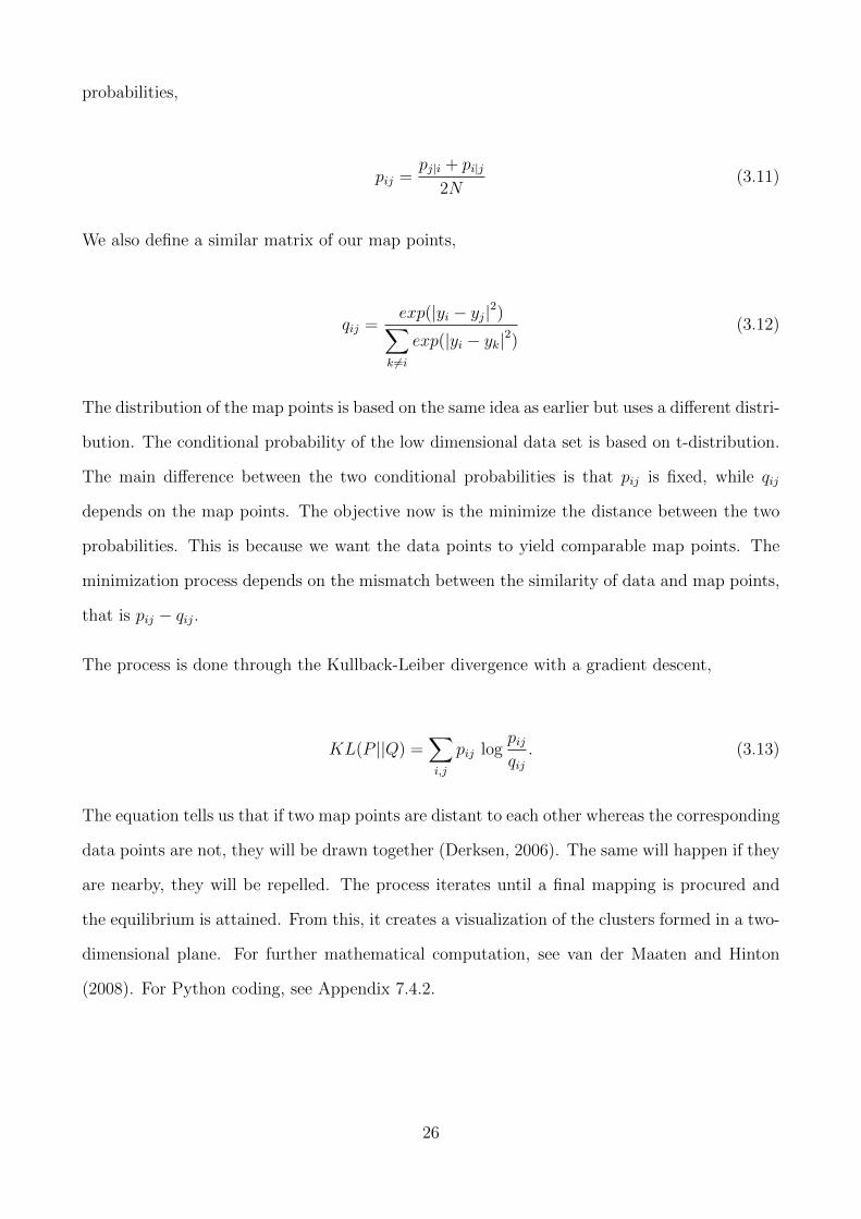
The distribution of the map points is based on the same idea as earlier but uses a different distri-
bution. The conditional probability of the low dimensional data set is based on t-distribution.
The main difference between the two conditional probabilities is that pij is fixed, while qij
depends on the map points. The objective now is the minimize the distance between the two
probabilities. This is because we want the data points to yield comparable map points. The
minimization process depends on the mismatch between the similarity of data and map points,
that is pij − qij.
The process is done through the Kullback-Leiber divergence with a gradient descent,
KL(P ||Q) =∑i,j
pij logpijqij. (3.13)
The equation tells us that if two map points are distant to each other whereas the corresponding
data points are not, they will be drawn together (Derksen, 2006). The same will happen if they
are nearby, they will be repelled. The process iterates until a final mapping is procured and
the equilibrium is attained. From this, it creates a visualization of the clusters formed in a two-
dimensional plane. For further mathematical computation, see van der Maaten and Hinton
(2008). For Python coding, see Appendix 7.4.2.
26
3.4 Stage 3: Identifying Mean-Reversion
In the third stage of our research design, we seek to find mean-reversion among stocks in the
clusters discovered in the previous stage. This will be identified by cointegration. Below is a
description of the elements regarding cointegration.
3.4.1 The Cointegration Approach
In this thesis, the cointegration approach for pairs trading has been chosen, following the
framework of Vidyamurthy (2004).
Stationarity
A time series is stationary when the parameters of the underlying data do not change over
time (Wooldridge, 2009). Wooldridge (2009) describes stationary as a stochastic process xt ∈
t = 1, 2... where every moment in time, the joint distribution of (x1, x2, ..., xm) is the same as
the joint distribution of (x1+h, x2+h, ..., xm+h) for all integers h ≥ 1. The definition is referred
to as a strict stochastic stationary process. Nevertheless, a weaker form of stationarity is more
commonly applied in finance due to its practical application on data samples. On this basis,
this thesis will engage in a weak stochastic stationary process. The process is weak stationary
if, for all values, the following is true:
• E(Yi(t)) = µ (Constant mean)
• var(Yi(t)) = σ2 (Constant variance)
• cov(Yi(t), Yi+s(t) = cov(yt, yi−s(t)) = γ (Covariance depends on s, not t)
The weak form of a stochastic stationary process needs to have constant mean and variance.
The most important feature is that the process has a constant mean. If the spread between
the stock pair deviates from the mean, we can capitalize by trading on this. Furthermore,
27
Wooldridge (2009) outlines that the covariance only concentrates on the first two moments of
a stochastic process. Hence, the structure does not change over time.
Non-stationary time series is referred to as random walks or random walks with a drift (Wooldridge,
2009). Random walks slowly wander upwards or downwards, but with no real pattern, while
random walks with a drift show a definite trend either upwards or downwards. As a rule of
thumb, non-stationary time series variables, which stock price series often are, should not be
used in regression models, in order to avoid spurious regression. However, most time series can
be transformed into a stationary process. This is done by differencing the time series, in such a
way that the values projects change and not absolute values. If a time series becomes stationary
after d times, it is referred to as an I(d). If Yi(t) and Xi(t) are non-stationary I(1) variables,
and a linear combination of them Si(t) = Yi(t)−βXi(t)−α is a stationary I(0) process (i.e. the
spread is stationary), then the set of Yi(t) and Xi(t) time series are cointegrated (Wooldridge,
2009).
Cointegration
Cointegration implies that Yi(t) and Xi(t) share similar stochastic trends, and since they both
are I(1) they never diverge too far from each other. The cointegrated variables exhibits a long-
term equilibrium relationship defined by Yi(t) = α+βXi(t) + Si(t), where Si(t) is the equlibrium
error, which represents short-term deviations from the long-term relationship (Wooldridge,
2009).
For pairs trading, the intuition is that if we find two stocks Yi(t) and Xi(t) that are I(1) and
whose prices are cointegrated, then any short-term deviations from the spread mean, Si, can be
an opportunity to place trades accordingly, as we bet on the relationship to be mean reverting.
When testing the spread for cointegration, we define the spread as,
Si(t) = Yi(t)− βXi(t) + αi (3.14)
28
When testing for cointegration, the Engle-Granger two-step method has been used1.
• Two steps in the Engle-Granger method:
1. Estimate the cointegration relationship using OLS.
2. Test the spread for stationarity
The Augmented-Dickey-Fuller (ADF) test2 is used to verify cointegration. Below is the general
formulation of the ADF test:
∆Si(t) = α + βt+ γSi(t−1) + δ1∆Si(t−1) +k∑i=1
θi∆St−i + εt, (3.15)
In our approach, the model of order 1 has been kept for all stock pairs. In addition, the ADF
statistics depends on whether an intercept and/or a linear trend are included (MacKinnon,
2010). The pairs trading strategy involves taking positions in the stock themselves, therefore
the intercept term is excluded. Thus, the ADF formulation we use is the following:
∆St = γSt−1 + θ∆St−1 + εt (3.16)
The null hypothesis is that there is no cointegration, the alternative hypothesis is that there
is a cointegrated relationship. If the p-value is small, below 5%, we reject the hypothesis that
there is no cointegrated relationship.
• Test: γ coefficient p-values:
– If γ p-value < 0.05: stationary time series with 95% of statistical confidence.
– if γ p-value > 0.05: time series non-stationary with 95% of statistical confidence.
1For a detailed description of the method, see (Engle and Granger, 1987)2For detailed information see (Dickey and Fuller, 1979)
29
3.5 Stage 4: Trading Setup and Execution
In the final stage of our research design, we seek to execute the trading algorithm and evaluate
the results. As stated in several studies, the general rule is to trade the positions when they
exceed a certain threshold. In this thesis, we have followed a similar trading procedure as
proposed by Caldeira and Moura (2013) and Avellaneda and Lee (2008).
3.5.1 Trading Signals and Execution
In the trading strategy, we focus on the spread-process Si(t) (3.14), but as aforementioned
neglecting the intercept term αi. This is because we only take position in the stocks themselves,
Yi(t) and Xi(t) accordingly. As described by Perlin (2009), a z-score is generated,
Zi =Si(t)− Siσeq,i
(3.17)
where,
Si =1
w
i−1∑j=i−w
Si(t) (3.18)
The z-score tells us the distance from the equilibrium spread in units of the equilibrium standard
deviation. The z-score is used for generating trading signals and positions. In this thesis, we
will utilize a rolling z-score to capture shifts in the spread. According to Reverre (2001) the
length of the rolling-window should be short enough to be reactive to shifts and long enough
to appear reasonably efficient in stripping noise out. On this basis and the fact that we are
trading on a six months basis, we have settled on a 10-day rolling z-score (w=10). Once 10
days of information is gathered, the trading algorithm begins. On that basis, we analyze if the
z-score is inside or outside the trading thresholds. This means that the portfolio is re-balanced
with 10 days of historical data.
30
The trading strategy is described as follows,
• Long Spread Trade:
– Enter long position: Previous (Z-Score > - 2) −− > Current (Z-Score < -2).
– Exit long position: Previous (Z-Score < +1) −− > Current (Z-Score > -1).
• Short Spread Trade:
– Enter short position: Previous (Z-Score < + 2) −− > Current (Z-Score > +2).
– Exit short position: Previous (Z-Score > +1) −− > Current (Z-Score < + 1).
We enter a trade position when the z-score exceeds ±2 and closes the position when it drops
below +1, and above −1 which is similar to Gatev et al. (2006), Andrade et al. (2005) and
Do and Faff (2010). The reason for trading within these thresholds are as follows: when the
z-score is far away from its equilibrium, we have reason to believe it will drift back again to
its equilibrium (because the spread was stationary in the past). On the other side, closing the
trade when the score passes the lower bound also makes sense since most stocks have some
sort of deviations. The portfolio is rebalanced every day to maintain the desired level of asset
allocation from our rolling z-score. If two stocks in a pair suddenly drift in opposite directions,
the portfolio can end up with significant risk exposure. We, therefore, rebalance our portfolio
as a mean to ensure that the portfolio is close to market-neutral, as documented by Do and
Faff (2010). For algorithmic development, see Appendix 7.4.4.
3.5.2 Training and Testing Periods
When testing a trading algorithm on historical data, it is crucial to reserve a time period for
testing purposes because it gives us an opportunity to see how the model would have performed
in a real-life situation. That is why we have divided the sample period into training (in-sample)
and testing (out-of-sample) periods.
31
In this thesis, we use a one year window for the training period and six months for the testing
period. This sums up to eight training and testing periods in total. The length of training
and backtesting periods is similar to the approach done by Caldeira and Moura (2013). When
deciding the duration of the training and testing periods, there is no finite answer. One should
make sure that the training period is long enough to determine if a cointegrated relationship
exists between the stocks. Similarly, the testing period should be long enough for trading
opportunities to occur.
The first training period is the year of 2013. Immediately after this period, the first test period
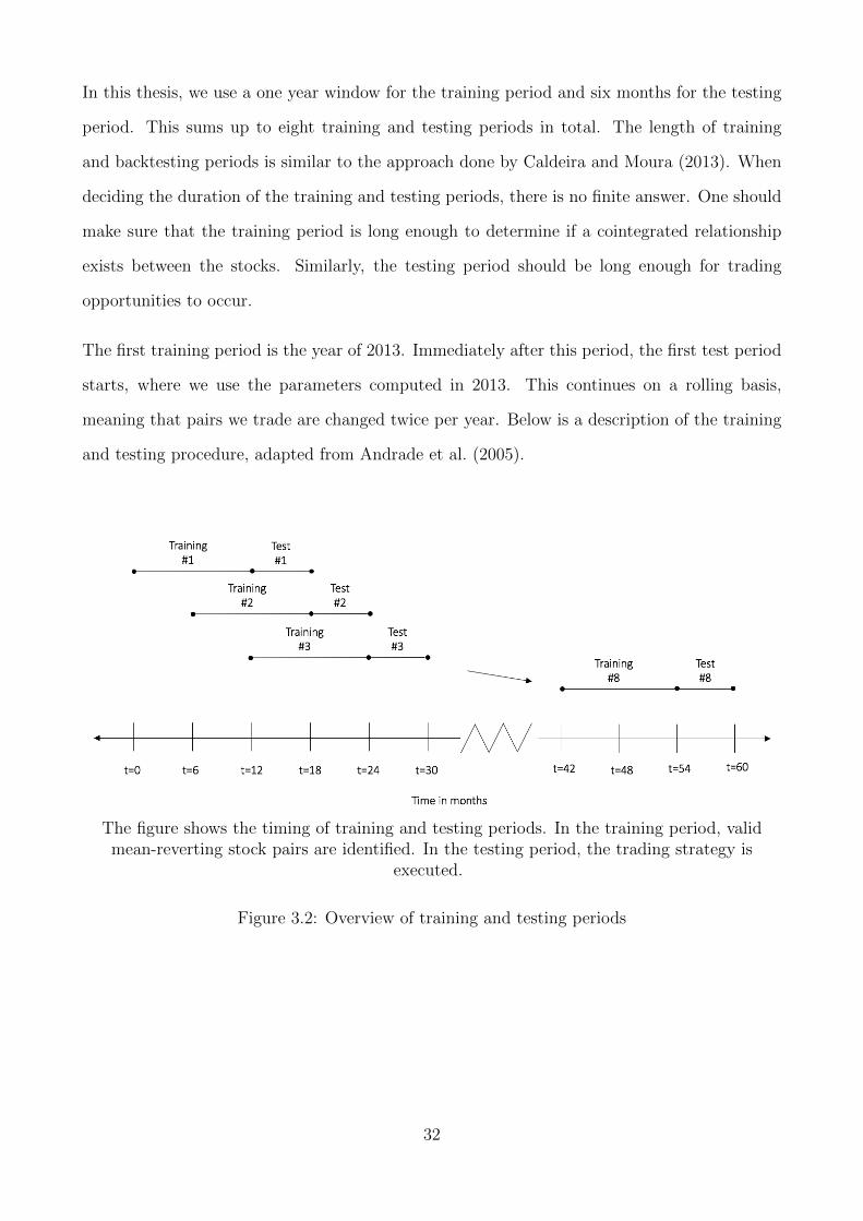
starts, where we use the parameters computed in 2013. This continues on a rolling basis,
meaning that pairs we trade are changed twice per year. Below is a description of the training
and testing procedure, adapted from Andrade et al. (2005).
The figure shows the timing of training and testing periods. In the training period, validmean-reverting stock pairs are identified. In the testing period, the trading strategy is
executed.
Figure 3.2: Overview of training and testing periods
32
3.5.3 Transaction costs
In order to correctly assess the performance of the pairs trading strategy, the impact of transac-
tion costs must be taken into consideration. According to Thapa and Sunil (2010), transaction
costs are decomposed into commission, fees, and slippage. However, since we are trading on
adjusted closing prices, we can disregard any slippage fees. Using the price model of Nordnet,
one of the largest trading platforms in Norway, the commission is settled at 4.9 basis points
(BPS) and fees at 0.25 BPS (Nordnet, 2018). In pairs trading, the simultaneous opening of a
long- and short position means transaction costs are occurring twice, thus commission is settled
at 9.8 BPS and fees at 0.5 BPS.
In addition, we have included short-sale rental costs as mentioned in Caldeira and Moura (2013).
In the Norwegian equity market, the annual short fee rate is 450 BPS (Nordnet, 2018). There
are 250 trading days per year, which gives us a daily shortage fee of 1.8 BPS. From the training
period analysis, we estimated an average trading position to last four days. This gives us an
average shortage fee of 7.2 BPS for each position. However, since shortage fees are only paid
when closing a position, this cost should not be included when entering a position. Thus, we
divide the shortage fee by two to represent the average trading cost1. This gives a rental fee of
3.6 BPS per trade. Assuming a continuation of this property for the testing periods, the total
transaction cost is 13.9 BPS (0.139%) per trade for every stock pair.
In this thesis, we have decided to disregard the fixed costs of NOK 250 per short position
(Nordnet, 2018) and tax implications. The fixed costs are in this model insignificant to the
overall returns and, taxes will be pertaining any profit no matter what the revenue stream.
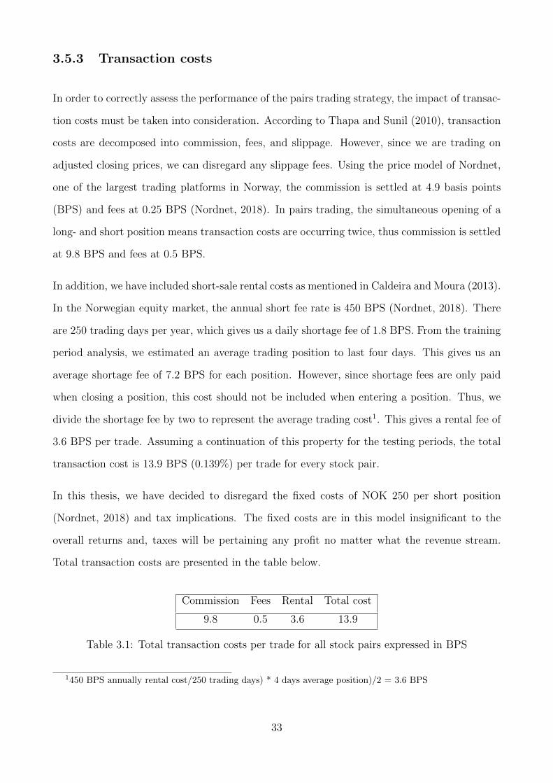
Total transaction costs are presented in the table below.
Commission Fees Rental Total cost
9.8 0.5 3.6 13.9
Table 3.1: Total transaction costs per trade for all stock pairs expressed in BPS
1450 BPS annually rental cost/250 trading days) * 4 days average position)/2 = 3.6 BPS
33
3.5.4 Performance Measures and Hypothesis Testing
The return metric used is the nominally change in NOK of each stock pairs over the testing
period. All stock pairs that were identified as cointegrated, will make up an equally weighted
portfolio. In addition, the risk is defined as fluctuations in stock pairs returns measured by its
standard deviation. This allows us to apply the Sharpe ratio (SR), as defined by,
SRi =Ri −Rf
σi(3.19)
with Ri denoting the return of a stock pair, and Rf the risk-free rate. The risk-free rate is
incorporated as 10-year Norwegian government bond with 1,95 % p.a as of 18.04.2018 (Norwe-
gian Central Bank, 2018). The standard deviation of a pair is denoted with σi. The Sharpe
ratio is measuring the risk premium per unit of risk (Bodie et al., 2014)
Apart from Sharpe ratio, we also present the measure of alpha, α, as obtained from the Capital
Asset Pricing Model (CAPM). The theory states that one can only obtain excess return if one
is willing to take risk. As according to Markowitz (1953), this can only be acquired by bearing
systematic or market risk. The theory describes the relationship between risk and reward as,
E[Ri]−Rf = βi(E[Rm]−Rf ) (3.20)
where βi = Cov(Ri,Rm)
σ2M
and E[Rm] denotes the expected market return. The βi denotes the
covariance between our stock pair and the market, over the market variance. This tells us
that βi describes the systematic risk captured by our stock pair. So, on the basis of CAPM, it
gives us a relationship between the expected excess return and risk premium. Knowing this,
we rearrange (3.20) to obtain the alpha,
αi = E[Ri]−Rf − βi(E[Rm]−Rf ) (3.21)
The alpha tells us how much better or worse our pairs trading strategy performed relative to
its benchmark i.e how well it performed relative to other securities with similar risk exposure.
34

That is why this metric can be used to determine whether our strategy is able to generate excess
return. On this premises, to see if there are arbitrage opportunities, we impose the following
hypothesis:
H0: There are no arbitrage opportunities
H1: There are arbitrage opportunities
We will utilize a one sample t-test to conclude whether there is arbitrage and to see if the
strategy provided excess return. Since we are concerned with positive excess return only, we
will employ a one-sided t-distribution.
35
3.6 Research Design Review
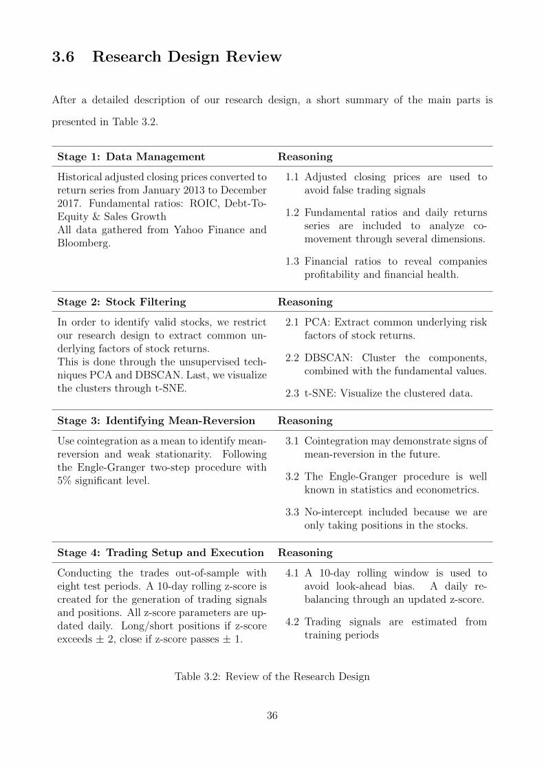
After a detailed description of our research design, a short summary of the main parts is
presented in Table 3.2.
Stage 1: Data Management Reasoning
Historical adjusted closing prices converted toreturn series from January 2013 to December2017. Fundamental ratios: ROIC, Debt-To-Equity & Sales GrowthAll data gathered from Yahoo Finance andBloomberg.
1.1 Adjusted closing prices are used toavoid false trading signals
1.2 Fundamental ratios and daily returnsseries are included to analyze co-movement through several dimensions.
1.3 Financial ratios to reveal companiesprofitability and financial health.
Stage 2: Stock Filtering Reasoning
In order to identify valid stocks, we restrictour research design to extract common un-derlying factors of stock returns.This is done through the unsupervised tech-niques PCA and DBSCAN. Last, we visualizethe clusters through t-SNE.
2.1 PCA: Extract common underlying riskfactors of stock returns.
2.2 DBSCAN: Cluster the components,combined with the fundamental values.
2.3 t-SNE: Visualize the clustered data.
Stage 3: Identifying Mean-Reversion Reasoning
Use cointegration as a mean to identify mean-reversion and weak stationarity. Followingthe Engle-Granger two-step procedure with5% significant level.
3.1 Cointegration may demonstrate signs ofmean-reversion in the future.
3.2 The Engle-Granger procedure is wellknown in statistics and econometrics.
3.3 No-intercept included because we areonly taking positions in the stocks.
Stage 4: Trading Setup and Execution Reasoning
Conducting the trades out-of-sample witheight test periods. A 10-day rolling z-score iscreated for the generation of trading signalsand positions. All z-score parameters are up-dated daily. Long/short positions if z-scoreexceeds ± 2, close if z-score passes ± 1.
4.1 A 10-day rolling window is used toavoid look-ahead bias. A daily re-balancing through an updated z-score.
4.2 Trading signals are estimated fromtraining periods
Table 3.2: Review of the Research Design
36
Chapter 4
Results
4.1 Determining the Number of Principal Components
The result from the PCA is presented in Figure 4.1. The figure describes the results from
training period 1. In the screen plot to the left, we can see the proportion of variance explained
by each of the principal components. On the right, we can see the cumulative proportion of
variance explained.
Along the y-axis is the proportion of variance explained, as explained by equation (3.9). Re-
member that we standardized our data in the stock filtering process, which means that each
variable has a mean of zero and variance of one. Because they have been standardized, each
variable contributes to one unit of variance to the total variance in the data.
From Figure 4.1, we can see that the first five components explain roughly 40 % of the total
variance, while 33 of the components (of the 50 total) is necessary to capture 95% of the variance.
Not surprisingly, the proportion of variance explained exhibits a logarithmic relationship with
the number of components which means that the marginal explanation of each component is
diminishing. This is because each component can be seen as representing a risk factor and it is
natural to think that different risk factors have different impact of the variance. Furthermore,
the first component is similar to the market risk (Avellaneda and Lee, 2008). For further
visualization of the first principal component, see Appendix 7.5.
37
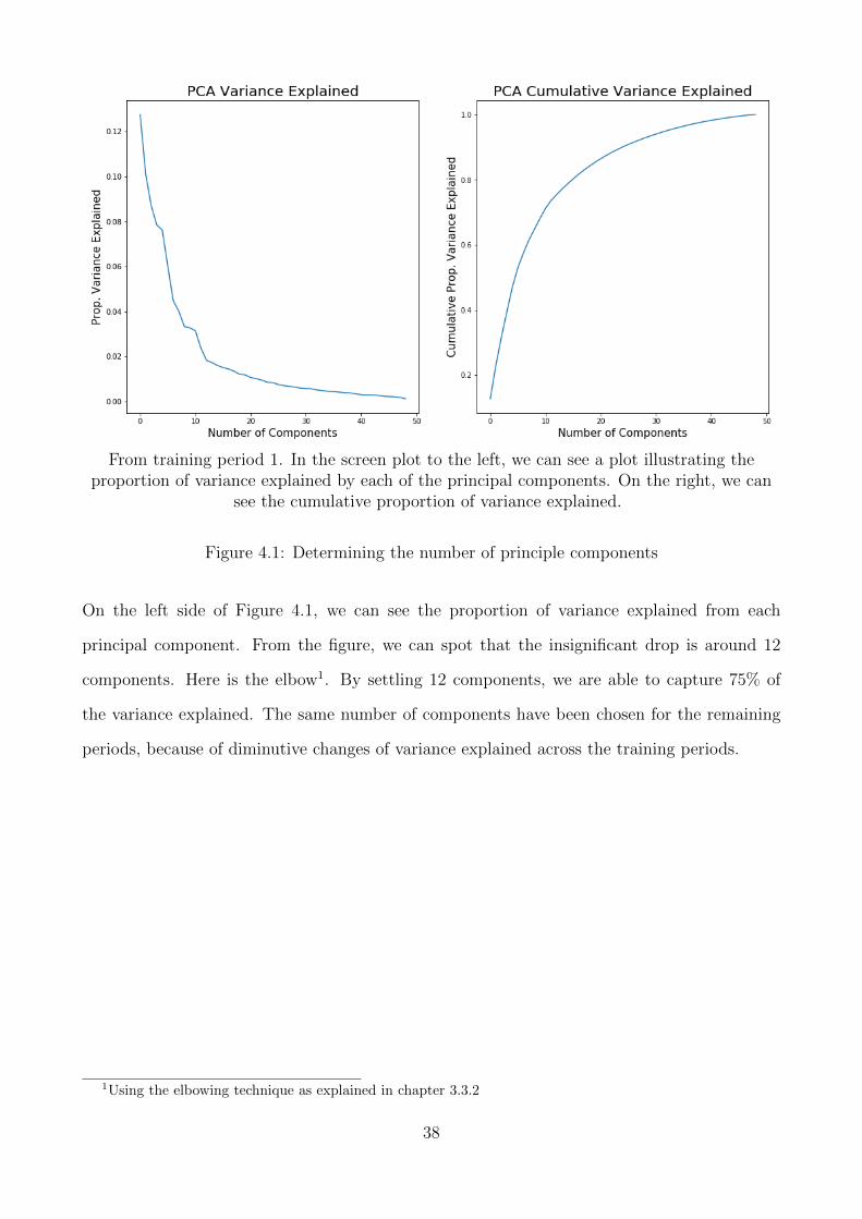
From training period 1. In the screen plot to the left, we can see a plot illustrating theproportion of variance explained by each of the principal components. On the right, we can
see the cumulative proportion of variance explained.
Figure 4.1: Determining the number of principle components
On the left side of Figure 4.1, we can see the proportion of variance explained from each
principal component. From the figure, we can spot that the insignificant drop is around 12
components. Here is the elbow1. By settling 12 components, we are able to capture 75% of
the variance explained. The same number of components have been chosen for the remaining
periods, because of diminutive changes of variance explained across the training periods.
1Using the elbowing technique as explained in chapter 3.3.2
38

4.2 Cluster Discovering
Upon cluster analysis, we projected the new PCA subspace together with the financial ratios
into regions of high density. The radius of each clusters e, where settled to 1.5. After trial
and error, this number was chosen to find the point which minimized the maximum distance
to all cluster points. For the minimum number of points, we settled minPts to 3. This was
chosen because we wanted to ensure that stocks with similar risk profile was clustered together.
Although the number of clusters will vary by the choice of e and minPts, these values are chosen
for all periods to be consistent.
On the whole, we identified one or two clusters for every training period. The clusters did,
however, differ in size and content from each training period. When visualizing the clusters,
the t-SNE algorithm was implemented on the DBSCAN output, providing us with Figure 4.2.
For a detailed description of all clusters formed, see Appendix 7.3.
39
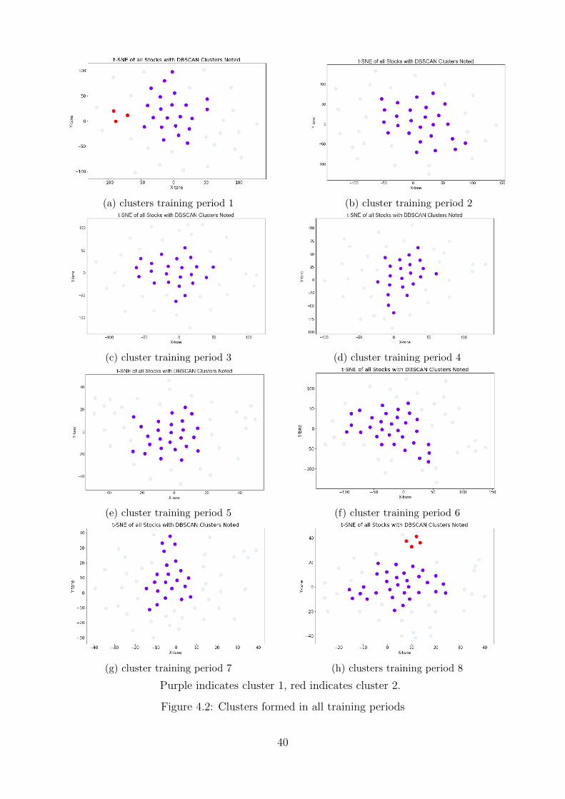
(a) clusters training period 1 (b) cluster training period 2
(c) cluster training period 3 (d) cluster training period 4
(e) cluster training period 5 (f) cluster training period 6
(g) cluster training period 7 (h) clusters training period 8
Purple indicates cluster 1, red indicates cluster 2.
Figure 4.2: Clusters formed in all training periods
40
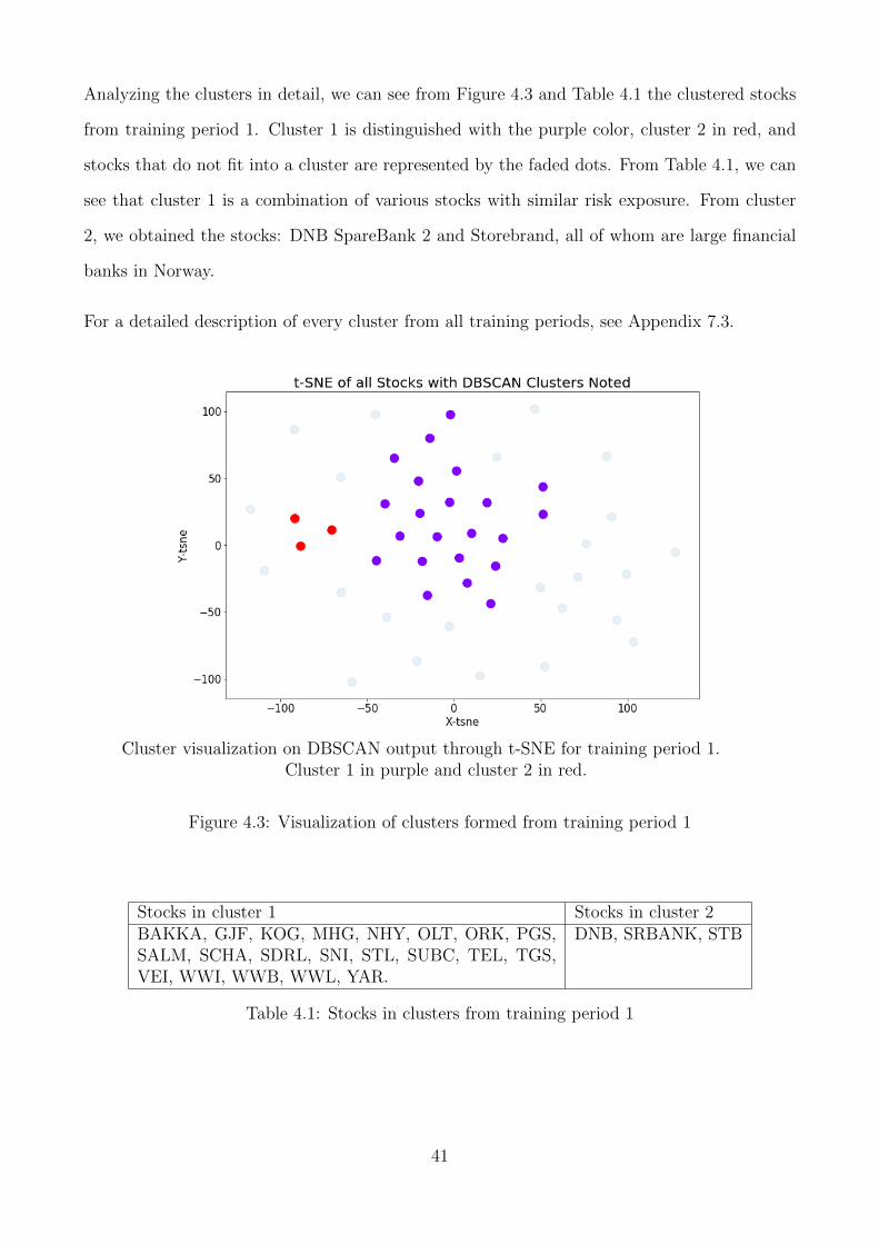
Analyzing the clusters in detail, we can see from Figure 4.3 and Table 4.1 the clustered stocks
from training period 1. Cluster 1 is distinguished with the purple color, cluster 2 in red, and
stocks that do not fit into a cluster are represented by the faded dots. From Table 4.1, we can
see that cluster 1 is a combination of various stocks with similar risk exposure. From cluster
2, we obtained the stocks: DNB SpareBank 2 and Storebrand, all of whom are large financial
banks in Norway.
For a detailed description of every cluster from all training periods, see Appendix 7.3.
Cluster visualization on DBSCAN output through t-SNE for training period 1.Cluster 1 in purple and cluster 2 in red.
Figure 4.3: Visualization of clusters formed from training period 1
Stocks in cluster 1 Stocks in cluster 2BAKKA, GJF, KOG, MHG, NHY, OLT, ORK, PGS,SALM, SCHA, SDRL, SNI, STL, SUBC, TEL, TGS,VEI, WWI, WWB, WWL, YAR.
DNB, SRBANK, STB
Table 4.1: Stocks in clusters from training period 1
41
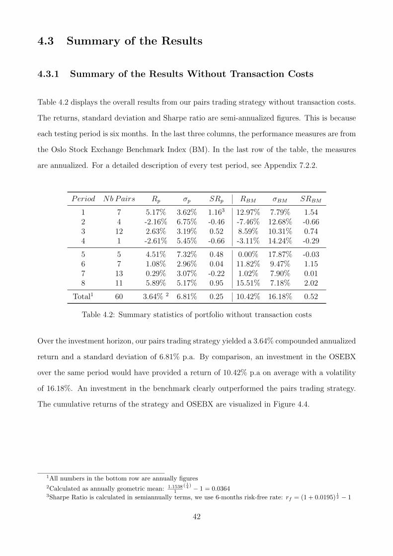
4.3 Summary of the Results
4.3.1 Summary of the Results Without Transaction Costs
Table 4.2 displays the overall results from our pairs trading strategy without transaction costs.
The returns, standard deviation and Sharpe ratio are semi-annualized figures. This is because
each testing period is six months. In the last three columns, the performance measures are from
the Oslo Stock Exchange Benchmark Index (BM). In the last row of the table, the measures
are annualized. For a detailed description of every test period, see Appendix 7.2.2.
Period Nb Pairs Rp σp SRp RBM σBM SRBM
1 7 5.17% 3.62% 1.163 12.97% 7.79% 1.542 4 -2.16% 6.75% -0.46 -7.46% 12.68% -0.663 12 2.63% 3.19% 0.52 8.59% 10.31% 0.744 1 -2.61% 5.45% -0.66 -3.11% 14.24% -0.29
5 5 4.51% 7.32% 0.48 0.00% 17.87% -0.036 7 1.08% 2.96% 0.04 11.82% 9.47% 1.157 13 0.29% 3.07% -0.22 1.02% 7.90% 0.018 11 5.89% 5.17% 0.95 15.51% 7.18% 2.02
Total1 60 3.64% 2 6.81% 0.25 10.42% 16.18% 0.52
Table 4.2: Summary statistics of portfolio without transaction costs
Over the investment horizon, our pairs trading strategy yielded a 3.64% compounded annualized
return and a standard deviation of 6.81% p.a. By comparison, an investment in the OSEBX
over the same period would have provided a return of 10.42% p.a on average with a volatility
of 16.18%. An investment in the benchmark clearly outperformed the pairs trading strategy.
The cumulative returns of the strategy and OSEBX are visualized in Figure 4.4.
1All numbers in the bottom row are annually figures2Calculated as annually geometric mean: 1.1538
1
( 14 ) − 1 = 0.0364
3Sharpe Ratio is calculated in semiannually terms, we use 6-months risk-free rate: rf = (1 + 0.0195)12 − 1
42
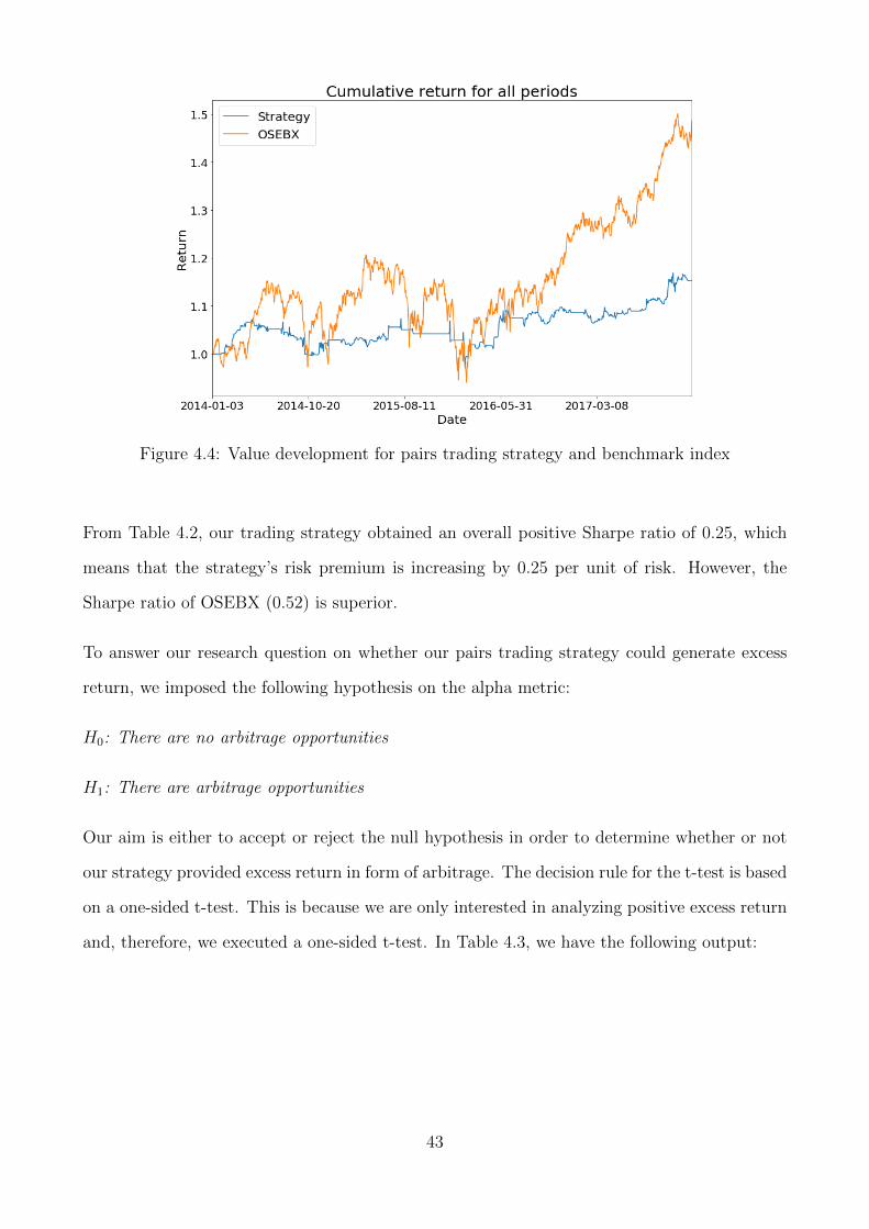
Figure 4.4: Value development for pairs trading strategy and benchmark index
From Table 4.2, our trading strategy obtained an overall positive Sharpe ratio of 0.25, which
means that the strategy’s risk premium is increasing by 0.25 per unit of risk. However, the
Sharpe ratio of OSEBX (0.52) is superior.
To answer our research question on whether our pairs trading strategy could generate excess
return, we imposed the following hypothesis on the alpha metric:
H0: There are no arbitrage opportunities
H1: There are arbitrage opportunities
Our aim is either to accept or reject the null hypothesis in order to determine whether or not
our strategy provided excess return in form of arbitrage. The decision rule for the t-test is based
on a one-sided t-test. This is because we are only interested in analyzing positive excess return
and, therefore, we executed a one-sided t-test. In Table 4.3, we have the following output:
43
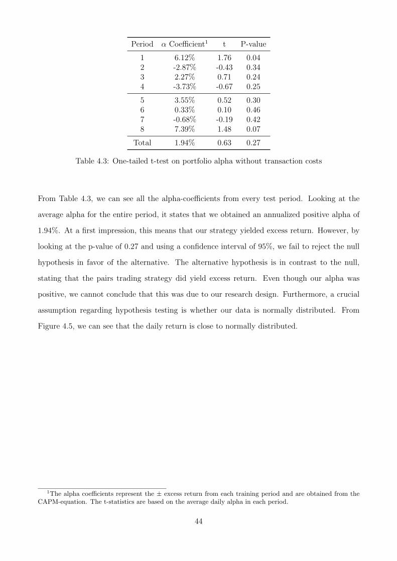
Period α Coefficient1 t P-value
1 6.12% 1.76 0.042 -2.87% -0.43 0.343 2.27% 0.71 0.244 -3.73% -0.67 0.25
5 3.55% 0.52 0.306 0.33% 0.10 0.467 -0.68% -0.19 0.428 7.39% 1.48 0.07
Total 1.94% 0.63 0.27
Table 4.3: One-tailed t-test on portfolio alpha without transaction costs
From Table 4.3, we can see all the alpha-coefficients from every test period. Looking at the
average alpha for the entire period, it states that we obtained an annualized positive alpha of
1.94%. At a first impression, this means that our strategy yielded excess return. However, by
looking at the p-value of 0.27 and using a confidence interval of 95%, we fail to reject the null
hypothesis in favor of the alternative. The alternative hypothesis is in contrast to the null,
stating that the pairs trading strategy did yield excess return. Even though our alpha was
positive, we cannot conclude that this was due to our research design. Furthermore, a crucial
assumption regarding hypothesis testing is whether our data is normally distributed. From
Figure 4.5, we can see that the daily return is close to normally distributed.
1The alpha coefficients represent the ± excess return from each training period and are obtained from theCAPM-equation. The t-statistics are based on the average daily alpha in each period.
44
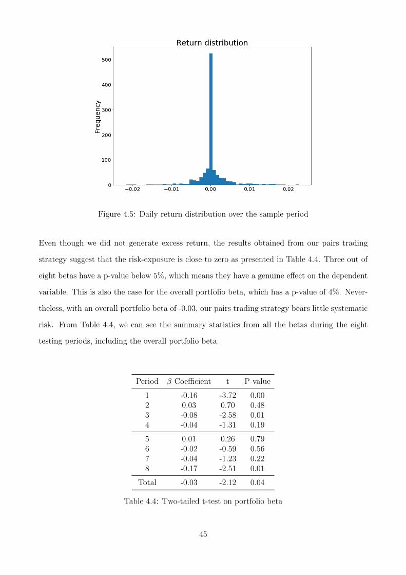
Figure 4.5: Daily return distribution over the sample period
Even though we did not generate excess return, the results obtained from our pairs trading
strategy suggest that the risk-exposure is close to zero as presented in Table 4.4. Three out of
eight betas have a p-value below 5%, which means they have a genuine effect on the dependent
variable. This is also the case for the overall portfolio beta, which has a p-value of 4%. Never-
theless, with an overall portfolio beta of -0.03, our pairs trading strategy bears little systematic
risk. From Table 4.4, we can see the summary statistics from all the betas during the eight
testing periods, including the overall portfolio beta.
Period β Coefficient t P-value
1 -0.16 -3.72 0.002 0.03 0.70 0.483 -0.08 -2.58 0.014 -0.04 -1.31 0.19
5 0.01 0.26 0.796 -0.02 -0.59 0.567 -0.04 -1.23 0.228 -0.17 -2.51 0.01
Total -0.03 -2.12 0.04
Table 4.4: Two-tailed t-test on portfolio beta
45
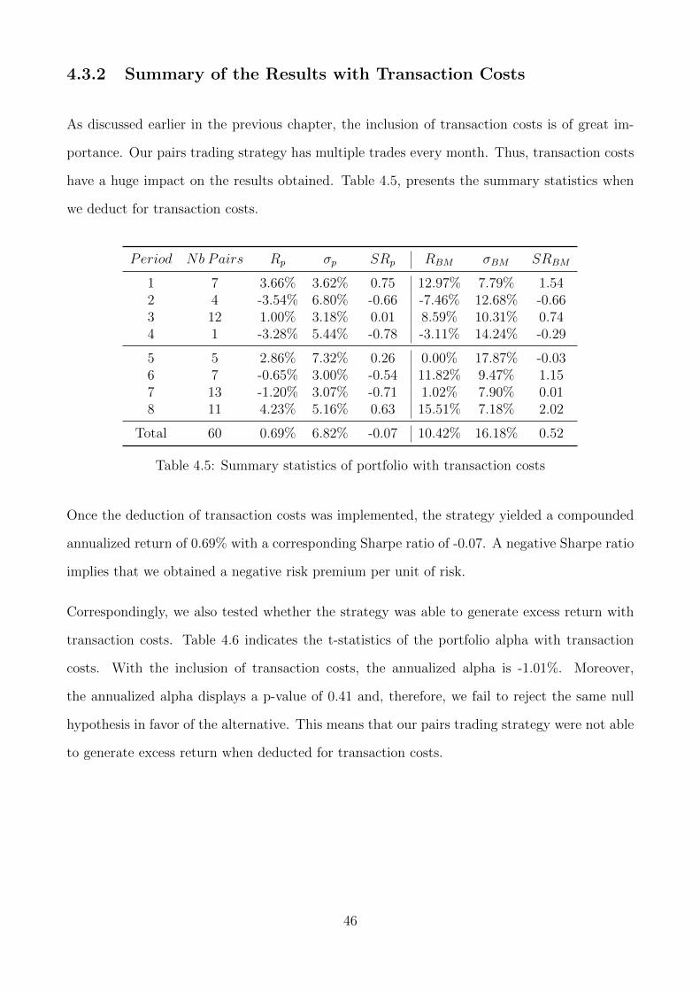
4.3.2 Summary of the Results with Transaction Costs
As discussed earlier in the previous chapter, the inclusion of transaction costs is of great im-
portance. Our pairs trading strategy has multiple trades every month. Thus, transaction costs
have a huge impact on the results obtained. Table 4.5, presents the summary statistics when
we deduct for transaction costs.
Period Nb Pairs Rp σp SRp RBM σBM SRBM
1 7 3.66% 3.62% 0.75 12.97% 7.79% 1.542 4 -3.54% 6.80% -0.66 -7.46% 12.68% -0.663 12 1.00% 3.18% 0.01 8.59% 10.31% 0.744 1 -3.28% 5.44% -0.78 -3.11% 14.24% -0.29
5 5 2.86% 7.32% 0.26 0.00% 17.87% -0.036 7 -0.65% 3.00% -0.54 11.82% 9.47% 1.157 13 -1.20% 3.07% -0.71 1.02% 7.90% 0.018 11 4.23% 5.16% 0.63 15.51% 7.18% 2.02
Total 60 0.69% 6.82% -0.07 10.42% 16.18% 0.52
Table 4.5: Summary statistics of portfolio with transaction costs
Once the deduction of transaction costs was implemented, the strategy yielded a compounded
annualized return of 0.69% with a corresponding Sharpe ratio of -0.07. A negative Sharpe ratio
implies that we obtained a negative risk premium per unit of risk.
Correspondingly, we also tested whether the strategy was able to generate excess return with
transaction costs. Table 4.6 indicates the t-statistics of the portfolio alpha with transaction
costs. With the inclusion of transaction costs, the annualized alpha is -1.01%. Moreover,
the annualized alpha displays a p-value of 0.41 and, therefore, we fail to reject the same null
hypothesis in favor of the alternative. This means that our pairs trading strategy were not able
to generate excess return when deducted for transaction costs.
46
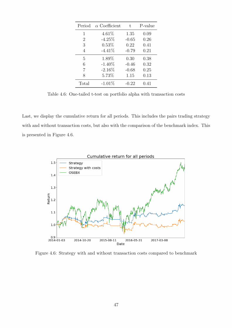
Period α Coefficient t P-value
1 4.61% 1.35 0.092 -4.25% -0.65 0.263 0.53% 0.22 0.414 -4.41% -0.79 0.21
5 1.89% 0.30 0.386 -1.40% -0.46 0.327 -2.16% -0.68 0.258 5.73% 1.15 0.13
Total -1.01% -0.22 0.41
Table 4.6: One-tailed t-test on portfolio alpha with transaction costs
Last, we display the cumulative return for all periods. This includes the pairs trading strategy
with and without transaction costs, but also with the comparison of the benchmark index. This
is presented in Figure 4.6.
Figure 4.6: Strategy with and without transaction costs compared to benchmark
47
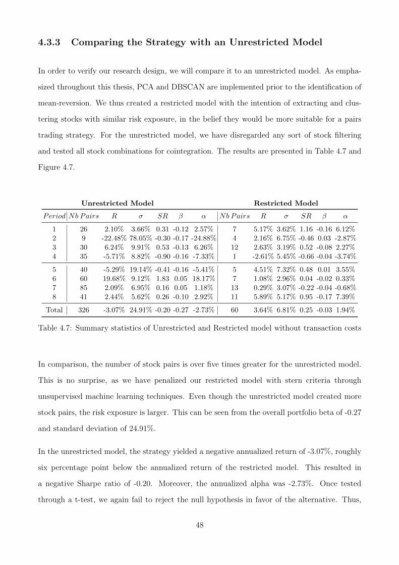
4.3.3 Comparing the Strategy with an Unrestricted Model
In order to verify our research design, we will compare it to an unrestricted model. As empha-
sized throughout this thesis, PCA and DBSCAN are implemented prior to the identification of
mean-reversion. We thus created a restricted model with the intention of extracting and clus-
tering stocks with similar risk exposure, in the belief they would be more suitable for a pairs
trading strategy. For the unrestricted model, we have disregarded any sort of stock filtering
and tested all stock combinations for cointegration. The results are presented in Table 4.7 and
Figure 4.7.
Unrestricted Model Restricted Model
Period Nb Pairs R σ SR β α Nb Pairs R σ SR β α
1 26 2.10% 3.66% 0.31 -0.12 2.57% 7 5.17% 3.62% 1.16 -0.16 6.12%2 9 -22.48% 78.05% -0.30 -0.17 -24.88% 4 2.16% 6.75% -0.46 0.03 -2.87%3 30 6.24% 9.91% 0.53 -0.13 6.26% 12 2.63% 3.19% 0.52 -0.08 2.27%4 35 -5.71% 8.82% -0.90 -0.16 -7.33% 1 -2.61% 5.45% -0.66 -0.04 -3.74%
5 40 -5.29% 19.14% -0.41 -0.16 -5.41% 5 4.51% 7.32% 0.48 0.01 3.55%6 60 19.68% 9.12% 1.83 0.05 18.17% 7 1.08% 2.96% 0.04 -0.02 0.33%7 85 2.09% 6.95% 0.16 0.05 1.18% 13 0.29% 3.07% -0.22 -0.04 -0.68%8 41 2.44% 5.62% 0.26 -0.10 2.92% 11 5.89% 5.17% 0.95 -0.17 7.39%
Total 326 -3.07% 24.91% -0.20 -0.27 -2.73% 60 3.64% 6.81% 0.25 -0.03 1.94%
Table 4.7: Summary statistics of Unrestricted and Restricted model without transaction costs
In comparison, the number of stock pairs is over five times greater for the unrestricted model.
This is no surprise, as we have penalized our restricted model with stern criteria through
unsupervised machine learning techniques. Even though the unrestricted model created more
stock pairs, the risk exposure is larger. This can be seen from the overall portfolio beta of -0.27
and standard deviation of 24.91%.
In the unrestricted model, the strategy yielded a negative annualized return of -3.07%, roughly
six percentage point below the annualized return of the restricted model. This resulted in
a negative Sharpe ratio of -0.20. Moreover, the annualized alpha was -2.73%. Once tested
through a t-test, we again fail to reject the null hypothesis in favor of the alternative. Thus,
48
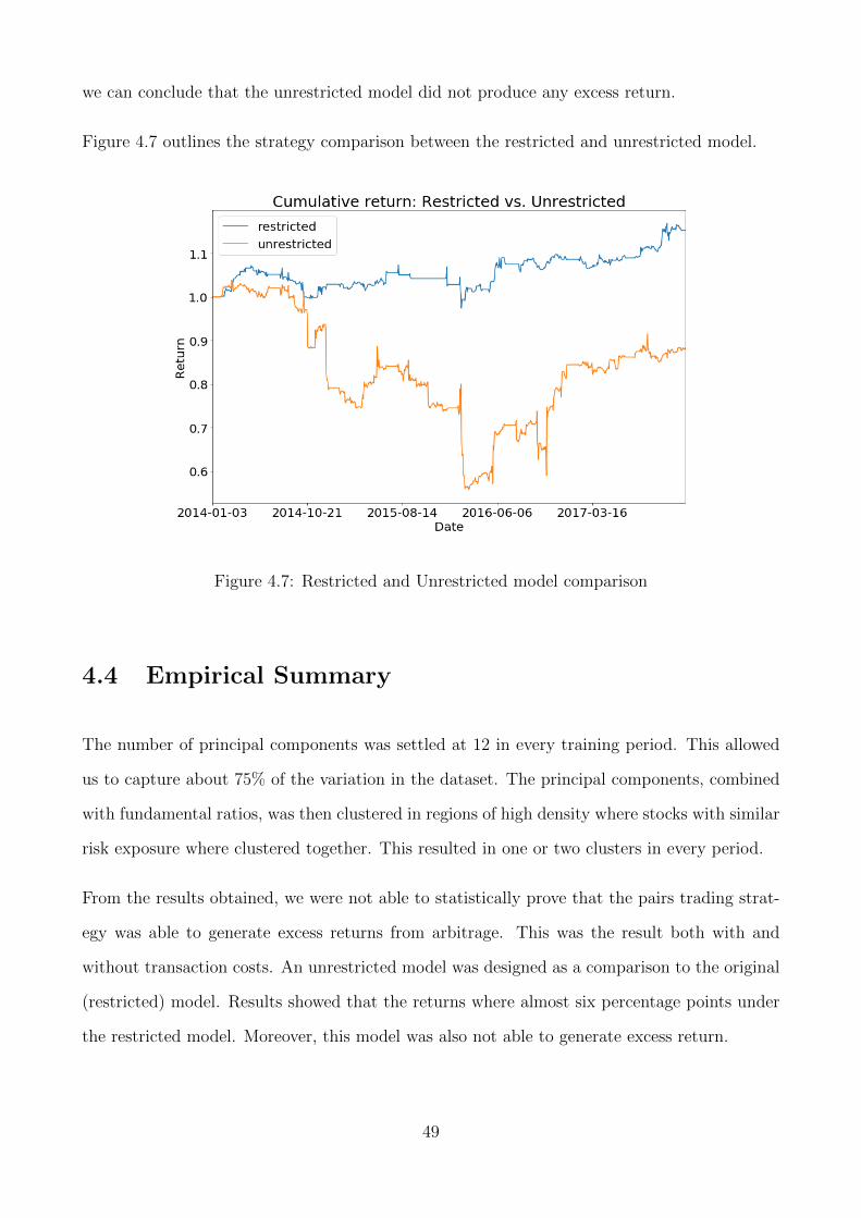
we can conclude that the unrestricted model did not produce any excess return.
Figure 4.7 outlines the strategy comparison between the restricted and unrestricted model.
Figure 4.7: Restricted and Unrestricted model comparison
4.4 Empirical Summary
The number of principal components was settled at 12 in every training period. This allowed
us to capture about 75% of the variation in the dataset. The principal components, combined
with fundamental ratios, was then clustered in regions of high density where stocks with similar
risk exposure where clustered together. This resulted in one or two clusters in every period.
From the results obtained, we were not able to statistically prove that the pairs trading strat-
egy was able to generate excess returns from arbitrage. This was the result both with and
without transaction costs. An unrestricted model was designed as a comparison to the original
(restricted) model. Results showed that the returns where almost six percentage points under
the restricted model. Moreover, this model was also not able to generate excess return.
49
Chapter 5
Discussion
In this chapter, we will try to reconnect the empirical findings with the outlined theoretical
frameworks. The main theoretical frameworks are the efficient-market hypothesis, the arbitrage
pricing theory, and pairs trading. We have therefore structured the discussion in this manner.
5.1 The Efficient-Market Hypothesis
The first theoretical point of departure was the efficient-market hypothesis (EMH), which stated
that the value of a transaction is at its correct value because all of the information is fully
reflected in the price (Fama, 1970). Moreover, the theory outlines the concept of no-arbitrage,
stating that stock prices follow a random walk and, as a consequence, one cannot exploit
mispricing of stocks. Our empirical results support this theory. The purpose of t-testing the
alpha of the portfolio was to determine if our statistical arbitrage strategy were able to generate
excess return on the Norwegian stock market. Even though we obtained an alpha of 1.94%,
we failed to reject the null hypothesis in favor of the alternative and the alpha was therefore
not statistically significant. Thus, our findings are in line with Fama (1970) and the EMH.
This means that changes in stock prices cannot be reflected in algorithms, while excess return
is gained as luck rather than an outcome of a correct prediction (Degutis and Novickyt, 2014).
Furthermore, our study leads to the questioning of exactly how efficient the Norwegian stock
50

market was during our sample period. As aforementioned, Fama (1970) outlines three kinds of
market efficiency based on the information set, namely the weak, semi-strong and strong. The
strong form postulates that all information, both public and private is reflected in the stock
price. It is hard to argue for the latter because this implies that stock prices also includes inside
information. Because of this uncertainty, the Norwegian stock market cannot be described as
having a strong market efficiency. On the contrary, we can conclude that the OSEBX is
an example of the weak-form efficiency since we were not able to generate excess return on
historical data. The question is whether we can characterize it to be on the semi-strong form,
where stock prices reflect both past and present public information. Bodie et al. (2011) argues
that the semi-strong form is where all investors do not interpret the information in the same way,
possibly leading to adverse situations from technical or fundamental analysis. We will, therefore,
conclude that the Norwegian stock market is at a semi-strong form because even though we
were not able to generate an overall positive portfolio alpha, there where some periods with
positive significant results, which gives indications that there are arbitrage opportunities every
now and then.
Looking at the empirical results from a broader perspective, we can see that investing in
an actively managed portfolio will not outperform the market. Since we conclude that the
Norwegian stock market is (semi-form) efficient, there is no incentive to spend resources to
gather information and trade on it. Looking at the evidence, there is not much research in
favor of active management. Some studies reveal that active management before cost may give
the same return as passive investing. However, when deducting for costs associated with active
management, it turns out that passive management gives the highest return (Fama and French,
2010), which is consistent with our results.
51
5.2 The Arbitrage Pricing Theory
Having discussed the results in light of the EMH, the second theoretical point of departure
was the Arbitrage Pricing Theory. In our pairs trading strategy, we sought to extract common
underlying risk factors of stock returns in the understanding that these could lead to more
robust cointegrated stock pairs. This was because the APT uncovered the heart of pairs trading
because it stated that stocks with similar risk exposure would yield the same return and, as
a consequence, one could use the APT theory as a catalyst to find mispriced stocks and place
trades accordingly (Harlacher, 2016).
In the pursuit of extracting the underlying risk factors, we used the principal component anal-
ysis to avoid ad hoc choices of factors. Nevertheless, in PCA, the components obtained are
uninterpretable because completely new variables are created in a new subspace. This means
that we have to trust that our research design is conducted in an adequate manner without
any form of misspecifications. Moreover, when deciding the number of factors (principal com-
ponents), we looked for the point at which the eigenvalues dropped and became insignificant,
namely an ad hoc choice of the number of factors. This could, therefore, bias our results in a
way that we captured too much or too little of the explained variance. Because almost half of
the cointegrated pairs ceased to exist out-of-sample, it gives us an indication that the number
and nature of the extracted factors were collected on false premises.
Notwithstanding, when we compared our strategy against the unrestricted model, it gives us
confidence that PCA and DBSCAN were able, to a certain degree, to filter out stocks suitable
for pairs trading. In the words of Avellaneda and Lee (2008), PCA decomposes and extract
risk components, as a way to sort out the idiosyncratic noise. Clearly, this is evident in the
restricted model when comparing it to the unrestricted model. Under those circumstances, we
can infer that the cointegrated relationship between the stocks in the unrestricted model has
further disintegrated out-of-sample compared to our restricted model. In this regard, we have
reason to believe that filtering out stocks by using unsupervised machine learning techniques and
including financial ratios are in fact beneficial when designing a statistical arbitrage strategy.
52

5.3 Pairs Trading
The last theoretical point of departure, was the empirical evidence of pairs trading. During our
investment horizon, a total of 60 pairs were traded, 35 of which ended with positive returns.
This proves that almost half of all pairs diverged more than desired out-of-sample and nega-
tively affected the overall performance. This confirms the unfavorable profits due to diverging
properties and advances in technology as documented by Do and Faff (2010). There may be
various reasons for declining profits, but we will outline three distinct motives presented in
previous literature, which we believe is relevant to our strategy.
1. First, a disintegration between two cointegrated stocks can be due to a structural shock or
break, as first outlined by Hamilton (1992). This means that the stocks are still inherently
cointegrated, but with different parameter values which our model is not able to capture.
2. Second, De Bondt and Thaler (1985) argue that stock returns have a tendency to reverse
itself over the long run. They call it the reversal effect, an effect in which losers rebound and
winners fade back. Thus, if our testing periods are too short, we may not be able to generate
profit from stock pairs that take longer to converge back to their long-term mean.
3. Last, the original article of Gatev et al. (1999), which has been in circulation for a long
time, may have contributed to a great enthusiasm for the use of pairs trading strategies among
sophisticated investors. Increased competition coupled with the development of technology,
might have vanished the profitability away.
In the light of pairs trading as a relative value investment, the strategy may, therefore, have
seen its glory days. As more and more investors use similar strategies and chase the same price
discrepancies, such mispricing will be eliminated more quickly, thus leading to lower returns.
Therefore, it does not come as a surprise that we were not able to achieve excess return.
As presented in the results, we found that our pairs trading strategy is close to market neutral
with an overall portfolio beta of -0.03, which is in accordance with Gatev et al. (2006). On
the contrary, we saw great fluctuations in the OSEBX over the sample period. This is likely
53

to be linked with the historical volatility in oil prices. Since the Norwegian stock market is
heavily exposed to the oil and gas industry, it is reasonable to assume that the high alteration
in the oil and gas industry was probably rippling over to other sectors, resulting in negative
repercussions and skepticism among equity investors at the OSEBX at the beginning of the
sample period.
Nevertheless, our pairs trading risk-exposure remained stable throughout the turmoil. It also
generated higher returns than the OSEBX in three out of the first five testing periods. This is
to some extent consistent with what we mentioned in the empirical evidence of pairs trading.
Namely that the strategy works particularly well in times of uncertainty and financial crises.
During such adverse situations, there is usually a shortage of liquidity which can cause stock
prices to deviate from its fundamental value. Stocks which usually follows the same stochas-
tic process can suddenly diverge because liquidity is of dire constraints in the market. Such
situations can be a good opportunity to increase pairs trading activities. By conducting pairs
trading in these situations, one can take the role as an intermediary or liquidity provider. This
is because we buy the underperforming stock and sell the stocks that do relatively well. Thus,
we can see that the return from our pairs trading strategy was negatively correlated in times of
financial turmoil, as outlined by Acharya and Pedersen (2005). From these findings, we believe
pairs trading can be used as a mean to hedge systematic risk, especially in times of financial
distress.
Although Do and Faff (2010) found declining profit in pairs trading, we hoped that the per-
formance of our strategy would match the results obtained by Avellaneda and Lee (2008) and
Avalon et al. (2017), which found favorable results with the use of unsupervised machine learn-
ing techniques. However, the studies of both (Avellaneda and Lee, 2008) and (Avalon et al.,
2017) were conducted on the S&P 500. This is considered to be the most liquid and traded stock
market in the world. It is, therefore, natural that such a strategy would yield different results
on the Norwegian stock market. A market with more homogeneous companies. Conducting
the algorithmic trading model as presented in this thesis may, therefore, be more beneficial for
a larger stock universe. With a larger stock universe, PCA and DBSCAN would most likely
result in a larger number of clusters, which again could provide more robust stock pairs.
54

5.4 Discussion Summary
Based on our analysis, the results are in accordance with the efficient-market hypothesis (EMH).
Even though we obtained a relative market-neutral strategy with a beta close to zero, we were
not able to gain a statistically significant excess return on the Norwegian stock market. With the
rise of algorithmic trading and advanced computerized systems to analyze stock movements,
we hoped to capitalize on market inefficiencies and asymmetric information on which such
technology could bring. On the contrary, because of the improved technological novelties, it
seems that the market is more efficient than we sought out. This means that the efficient-
market hypothesis relevancy is more present than ever and, as a consequence, we can conclude
that there is no such thing as a free lunch.
55
Chapter 6
Conclusion
6.1 Summary
At the beginning of this thesis, we outlined the idea of no-arbitrage saying that there is no
such thing as a free lunch. Determined to use statistical algorithms to find a free lunch on the
Norwegian stock market, we imposed the following research question:
Can algorithmic pairs trading with machine learning generate excess return?
Our main purpose was, therefore, to establish and create a pairs trading algorithm to capitalize
on market inefficiencies. In the seek of the research question we used three unsupervised
machine learning techniques to extract and cluster stocks with the same underlying risk factors.
Thereafter, we identified cointegration among the stocks and placed trades accordingly. Based
on the empirical results obtained, we can draw the following conclusion:
1. There seems not to be any arbitrage opportunities on the Norwegian stock market.
2. The stock market is efficient in the semi-strong form.
3. Pairs trading is a market-neutral strategy with almost no exposure to systematic risk
4. Unsupervised machine learning techniques have properties which are beneficial for a pairs
trading strategy
56
We found that the strategy is close to market neutral with a statistically significant beta value
of -0.03. Notwithstanding, with the implementation of transaction costs, the strategy only
obtained an alpha of -1.02% and return of 0.69% p.a. Thus, we statistically concluded that
pairs trading do not generate excess return on the Norwegian stock market in the sample period
from January 2013 to December 2017. This is in line with the efficient-market hypothesis.
Nevertheless, our strategy outperformed an unrestricted model based solely on cointegration.
This reveals that extracting common underlying factors of stock returns and cluster them into
regions of high density have properties that are beneficial for selecting stocks for a pairs trading
strategy. On these premises, we can, therefore, inform and verify: there is no such thing as a
free lunch.
6.2 Limitations and Future Work
One of the limitations of our research is that we have applied our research design on the
Norwegian stock market over a relatively short period of time. We only conclude that there
seems not to be any arbitrage on the Norwegian stock market in the given period. Longer or
other sample periods could have provided different conclusions. Second, we concluded to use
the same parameters in the machine learning algorithms for all periods. This could have biased
our results as periods most likely changes throughout time.
Furthermore, during our pairs trading analysis, we identified aspects which can be considered
in future work. We will outline the five aspects which we believe are the most relevant.
First, the strategy could be examined over a longer period or in two different decades. This
could potentially give us an indication if there is declining profitability of pairs trading on the
Norwegian stock market.
Second, since our strategy relies on cointegrated stocks in-sample, they may lose this relation-
ship out of sample. As a result, adding adaptive trading rules could be taken into account.
Adding a stop-loss function to our algorithm could probably make the strategy more robust.
57

Third, we assume that all stocks at the OSEBX are possible to short. This is not necessarily
always the case in real life due to the liquidity in the stock themselves. Therefore, adding
liquidity requirements to the model could be investigated in greater detail.
Fourth, in our thesis, we used adjusted closing prices since this is the common practice in
the pairs trading literature. Implementing intra-day prices instead of closing prices would
potentially give a more realistic view of the trade executions and transaction costs.
Last, the use of machine learning in pairs trading was very useful compared to an unrestricted
model. However, it did not help us to achieve excess returns. It would, therefore, be interesting
to see if other techniques would have provided better results. This could be through the use of
the supervised techniques Support Vector Machines or Neural Networks. In greater detail, these
techniques allow us to categorize unlabeled data and is one of the most widely used clustering
algorithms in industrial applications.
58
References
Acharya, V. and Pedersen, L. (2005). Asset pricing with liquidity risk. The Journal of Financial
Economics, 77:375–410.
Andrade, S. C., Pietro, V. d., and Seasholes, M. S. (2005). Understanding the Profitability of
Pairs Trading. UC Berkeley Working paper.
Avalon, G., Becich, M., Cao, V., Jeon, I., Misra, S., and Puzon, L. (2017). Multi-factor
Statistical Arbitrage Model. Stanford University.
Avellaneda, M. and Lee, J.-H. (2008). Statistical arbitrage in the u.s. equities market. Quan-
titative Finance, 10(7):761–782.
Avolio, G. D., Gildor, E., and Shleifer, A. (2002). Technology, information production, and
market efficiency. Economic Policy for the Information Economy. Federal Reserve Bank of
Kansas City.
Bjork, T. (1998). Arbitrage theory in continuous time. Oxford University Press Inc, Great
Clarendon Street, Oxford OX2 6DP.
Bodie, Z., Kane, A., and Marcus, A. (2011). Investments and Portfolio Management. McGraw
Hill/Irwin, New York.
Bodie, Z., Kane, A., and Marcus, A. (2014). Investments. McGraw-Hill Education, 2 Penn
Plaza, New York, NY 10121, 10th edition.
Bogomolov, T. (2013). Pairs trading based on statistical variability of the spread process.
Quantitative Finance, 13(9):1411–1430.
59
Broussard, J. P. and Vaihekoski, M. (2012). Profitability of pairs trading strategy in an illiq-
uid market with multiple share classes. The Journal of International Financial Markets,
22(5):1188–1201.
Caldeira, J. and Moura, G. (2013). Selection of a portfolio of pairs based on cointegration: A
statistical arbitrage strategy. Rev. Bras. Financas (Online), Rio de Janeiro, 11(1):49–80.
Chamberlain, G. and Rothschild, M. (1983). Arbitrage, factor structure, and mean-variance
analysis on large asset markets. Econometrica, 51:1281–304.
De Bondt, W. F. M. and Thaler, R. (1985). Does the stock market overreact? The Journal of
Finance, 40(3):361–372.
Degutis, A. and Novickyt, L. (2014). The efficient market hypothesis: A critical review of
literature and methodology. Ekonomika, 92(2).
Derksen, L. (2006). Visualising high-dimensional datasets using pca and t-sne in python.
Retrieved from: https://medium.com/@luckylwk/visualising-high-dimensional-datasets-
using-pca-and-t-sne-in-python-8ef87e7915b.
Dickey, D. A. and Fuller, W. A. (1979). Distribution of the estimators for autoregressive time
series with a unit root. Journal of the American Statistical Association.
Do, B.-H. and Faff, R. W. (2010). Does simple pairs trading still work? The Financial Analyst
Journal, 66(4):83–95.
Engle, R. and Granger, C. (1987). Co-integration and error correction: Representation, esti-
mation, and testing. Econometrica, 55(2):251–276.
Ester, M., Kriegel, H.-P., Sander, J., and Xu, X. (1996). A density-based algorithm for discov-
ering clusters in large spatial databases with noise. Proceedings of the Second International
Conference on Knowledge Discovery and Data Mining, 96:226–231.
Fama, E. F. (1970). Efficient capital markets: A review of theory and empirical work. The
Journal of Finance, 25(2):383–417.
60
Fama, E. F. and French, K. R. (2010). Luck versus skill in the crosssection of mutual fund
returns. The Journal of Financial, 65(5).
Gatev, E., Goetzmann, W. N., and Geert Rouwenhorst, K. (1999). Pairs trading: Performance
of a relative value arbitrage rule. Working paper, Yale School of Managements International
Center for Finance.
Gatev, E., Goetzmann, W. N., and Geert Rouwenhorst, K. (2006). Pairs trading: Performance
of a relative value arbitrage rule. Review of Financial Studies, 19(2):797–827.
Goulb, G. H. and Van Loan, C. F. (1996). Matrix Computations. The Johns Hopkins University
Press, 2715 North Charles Street.
Hamilton, J. D. (1992). Time Series Analysis. Princeton University Press, Princeton.
Harlacher, M. (2016). Cointegration Based Algorithmic Pairs Trading. PhD thesis, University
of St. Gallen.
Hogan, S., Jarrow, R., Teo, M., and Warachka, M. (2004). Testing market efficiency using
statistical arbitrage with applications to momentum and value strategies. The Journal of
Financial Economics, 73(3):525–565.
Jaeger, M. (2016). Dynamic cointegration based pairs trading. Master’s thesis, Copenhagen
Business School.
Jaju, S. (2017). Comprehensive guide on t-sne algorithm with implementation in r and python.
Retrieved from: https://www.analyticsvidhya.com/blog/2017/01/t-sne-implementation-r-
python/.
James, G., Witten, D., Travor, H., and Tibshirani, R. (2013). An Introduction to Statistical
Learning - with Applications in R. Springer, New York.
Jensen, M. (1978). Some anomalous evidence regarding market efficiency. The Journal of
Financial Economics, 6(2):95–101.
Jolliffe, I. (2002). Principal Component Analysis. Springer-Verlag, New York.
61
Kakushadze, Z. (2014). Mean-reversion and optimization. The Journal of Asset Management,
16(1):14–40.
Kim, D.-H. and Jeong, H. (2005). Systematic analysis of group identification in stocks markets.
The Physical Review, 72:046133.
Larkin, J. (2017). Pairs trading with machine learning. Quantopian Inc.
Retrieved from: https://www.quantopian.com/posts/pairs-trading-with-machine-learning.
Law, J. and Smullen, J. (2008). A Dictionary of Finance and Banking. Oxford University
Press, 4th edition.
Lazzarino, M., Berrill, J., and evi, A. (2018). What Is Statistical Arbitrage? Theoretical
Economics Letters, 8:888–908.
Lindstrom, E., Madsen, H., and Nielsen, J. N. (2015). Statistics for Finance. Taylor and Francis
Group.
Mackenzie, D. and Margenot, M. (2018). Introduction to pairs trading.
Retrieved from: https://www.quantopian.com/lectures/introduction-to-pairs-trading.
MacKinnon, J. G. (2010). Critical values for cointegration tests. Queens Economics Department
Working Paper No. 1227.
Madsen, R. E., Hansen, L. K., and Winther, O. (2004). Singular value decomposition
and principal component analysis. Technical report, Neural Networks. Retrieved from:
http://www2.imm.dtu.dk/pubdb/p.php?4000.
Malkiel, B. (2005). Reflections on the efficient market hypothesis: 30 years later. The Financial
Review, 40(1):1–9.
Markowitz, H. (1953). Portfolio selection. The Journal of Finance, 7(1):77–91.
Nordnet (2018). Prismodeller.
Retrieved from: https://www.nordnet.no/tjenester/prisliste.html.
62

Norwegian Central Bank (2018). Government bonds annual average.
Retrieved from: https://www.norges-bank.no/en/Statistics/Interest-rates/Government-
bonds-annual/.
Perlin, M. (2009). Evaluation of pairs trading strategy at the brazilian financial market. The
Journal of Derivatives and Hedge Funds, 15:122–136.
Pesaran, M. H. (2010). Predictability of asset returns and the efficient market hypothesis.
Discussion papaer, University of Cambridge.
Poitrast, G. (2010). Arbitrage: Historical perspectives. Encyclopedia of Quantitative Finance.
Poterba, J. and Summers, L. (1988). Mean reversion in stock prices: Evidence and implications.
The Journal of Financial Economics, 22:22–59.
Puntanen S., Styan G.P.H., I. J. (2011). Eigenvalue Decomposition. In: Matrix Tricks for
Linear Statistical Models. Springer, Berlin, Heidelberg.
Raschka, S. (2017). Python Machine Learning: Learning and Deep Learning with Python,
scikit-learn and TensorFlow. Packt, New York, 2nd edition.
Reverre, S. (2001). The Complete Arbitrage Deskbook. McGraw-Hill Education, 1st edition.
Rosenius, N. and Sjoholm, G. (2013). Arbitrage opportunities on the omxs: How to capitalize
on the ex-dividend effect. Master’s thesis, Ume School of Business and Economics.
Ross, S. (1975). The arbitrage theory of capital asset pricing. The Journal of Economic Theory,
13(3):341–360.
Sandberg, H. (2004). Model Reduction for Linear Time-Varing Systems. Department of Auto-
matic Control, Lund Institute of Technology (LTH).
Shukla, R. (1997). An empiricists guide to the arbitrage pricing theory. Syracuse University
Syracuse, NY 13244.
Tan, J. (2012). Principal component analysis and portfolio optimization. Available at SSRN:
https://ssrn.com/abstract=2213687 or http://dx.doi.org/10.2139/ssrn.2213687.
63
Thapa, C. and Sunil, S. P. (2010). International equity portfolio allocations and transaction
costs. The Journal of Banking and Finance, 34(11):2627–2638.
Timmermann, A. and Granger, C. W. (2004). Efficient market hypothesis and forecasting. The
International Journal of Forecasting, 20:15–27.
Trana, T. N., Nguyen, T. T., Willemsz, T. A., van Kessel, G., Frijlink, H. W., and van der
Voort Maarschalk, K. (2012). A density-based segmentation for 3d images, an application
for x-ray micro-tomography. Analytica Chimica Acta, 725:14–21.
van der Maaten, L. and Hinton, G. (2008). Visualizing data using t-sne. The Journal of
Machine Learning Research, 9:2579–2605.
Vidyamurthy, G. (2004). Pairs Tading: Quantitative Methods and Analysis. John Wiley and
Sons, Canada.
Wooldridge, J. M. (2009). Introductory Econometrics. South-Western Cengage Learning, 5191
Natorp Boulevard Mason, OH 45040 USA, 4th edition.
64
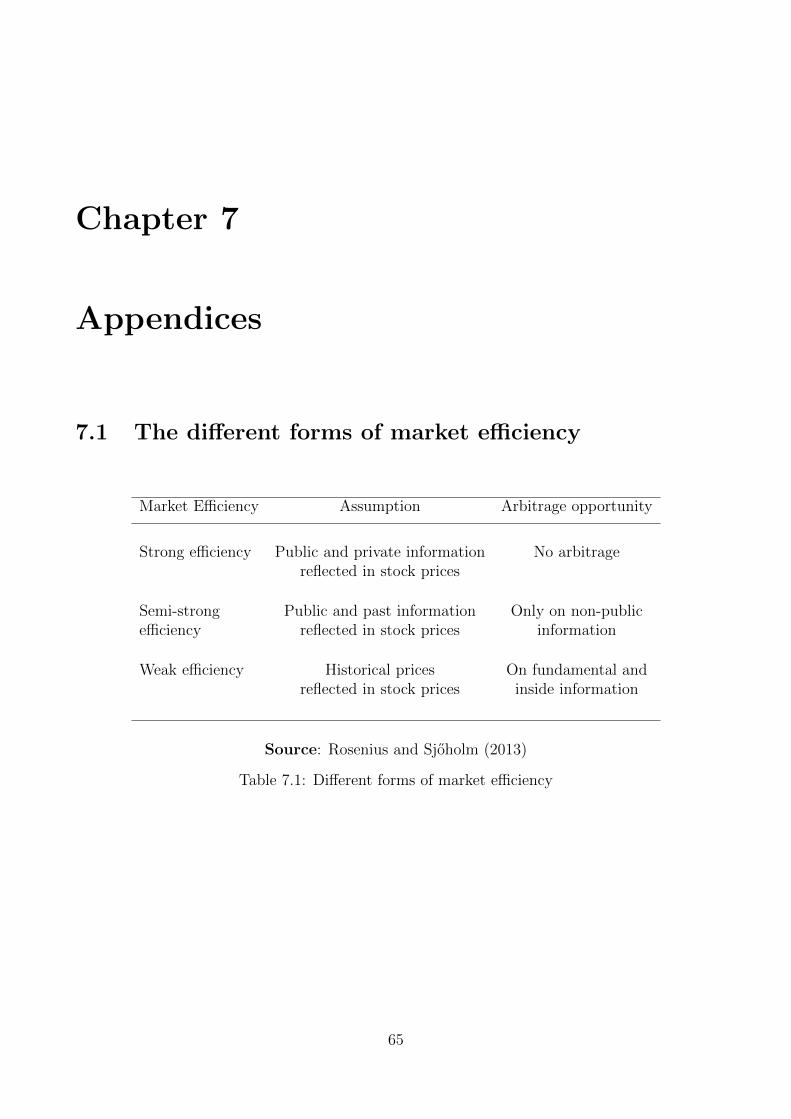
Chapter 7
Appendices
7.1 The different forms of market efficiency
Market Efficiency Assumption Arbitrage opportunity
Strong efficiency Public and private information No arbitragereflected in stock prices
Semi-strong Public and past information Only on non-publicefficiency reflected in stock prices information
Weak efficiency Historical prices On fundamental andreflected in stock prices inside information
Source: Rosenius and Sjoholm (2013)
Table 7.1: Different forms of market efficiency
65
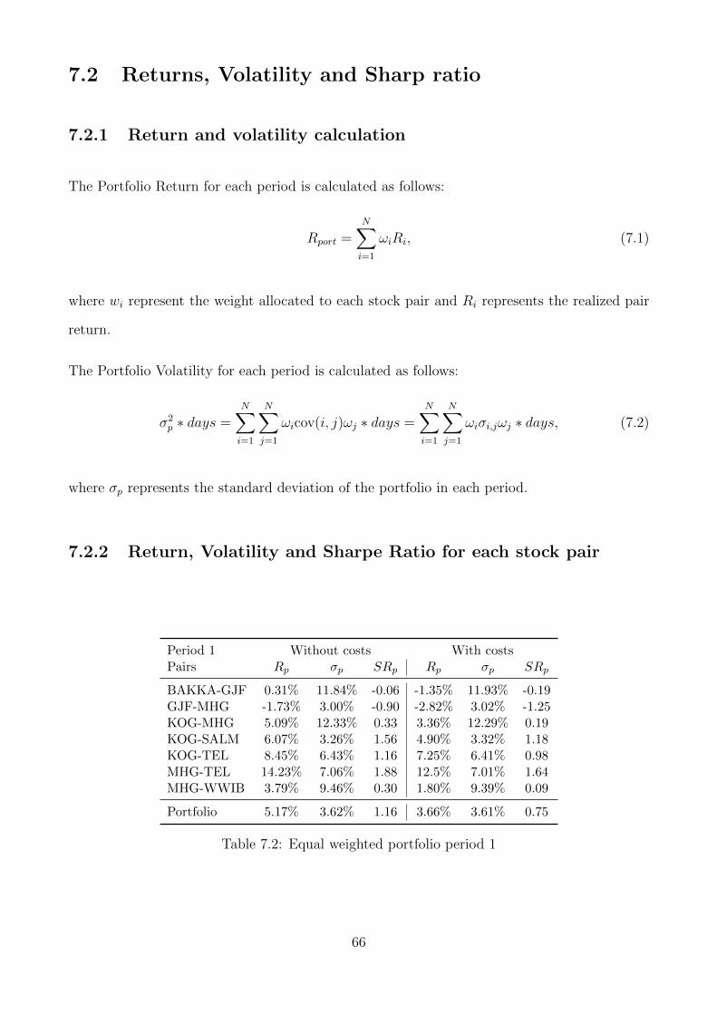
7.2 Returns, Volatility and Sharp ratio
7.2.1 Return and volatility calculation
The Portfolio Return for each period is calculated as follows:
Rport =N∑i=1
ωiRi, (7.1)
where wi represent the weight allocated to each stock pair and Ri represents the realized pair
return.
The Portfolio Volatility for each period is calculated as follows:
σ2p ∗ days =
N∑i=1
N∑j=1
ωicov(i, j)ωj ∗ days =N∑i=1
N∑j=1
ωiσi,jωj ∗ days, (7.2)
where σp represents the standard deviation of the portfolio in each period.
7.2.2 Return, Volatility and Sharpe Ratio for each stock pair
Period 1 Without costs With costsPairs Rp σp SRp Rp σp SRp
BAKKA-GJF 0.31% 11.84% -0.06 -1.35% 11.93% -0.19GJF-MHG -1.73% 3.00% -0.90 -2.82% 3.02% -1.25KOG-MHG 5.09% 12.33% 0.33 3.36% 12.29% 0.19KOG-SALM 6.07% 3.26% 1.56 4.90% 3.32% 1.18KOG-TEL 8.45% 6.43% 1.16 7.25% 6.41% 0.98MHG-TEL 14.23% 7.06% 1.88 12.5% 7.01% 1.64MHG-WWIB 3.79% 9.46% 0.30 1.80% 9.39% 0.09
Portfolio 5.17% 3.62% 1.16 3.66% 3.61% 0.75
Table 7.2: Equal weighted portfolio period 1
66
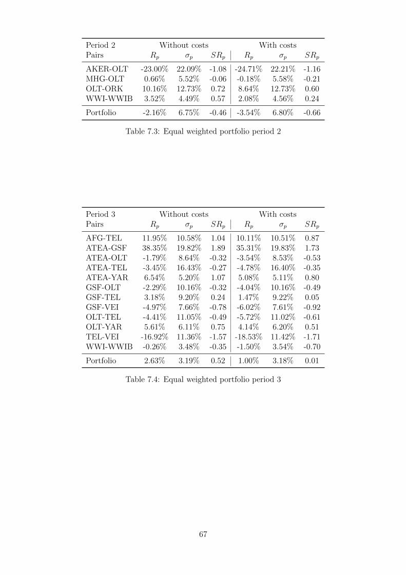
Period 2 Without costs With costsPairs Rp σp SRp Rp σp SRp
AKER-OLT -23.00% 22.09% -1.08 -24.71% 22.21% -1.16MHG-OLT 0.66% 5.52% -0.06 -0.18% 5.58% -0.21OLT-ORK 10.16% 12.73% 0.72 8.64% 12.73% 0.60WWI-WWIB 3.52% 4.49% 0.57 2.08% 4.56% 0.24
Portfolio -2.16% 6.75% -0.46 -3.54% 6.80% -0.66
Table 7.3: Equal weighted portfolio period 2
Period 3 Without costs With costsPairs Rp σp SRp Rp σp SRp
AFG-TEL 11.95% 10.58% 1.04 10.11% 10.51% 0.87ATEA-GSF 38.35% 19.82% 1.89 35.31% 19.83% 1.73ATEA-OLT -1.79% 8.64% -0.32 -3.54% 8.53% -0.53ATEA-TEL -3.45% 16.43% -0.27 -4.78% 16.40% -0.35ATEA-YAR 6.54% 5.20% 1.07 5.08% 5.11% 0.80GSF-OLT -2.29% 10.16% -0.32 -4.04% 10.16% -0.49GSF-TEL 3.18% 9.20% 0.24 1.47% 9.22% 0.05GSF-VEI -4.97% 7.66% -0.78 -6.02% 7.61% -0.92OLT-TEL -4.41% 11.05% -0.49 -5.72% 11.02% -0.61OLT-YAR 5.61% 6.11% 0.75 4.14% 6.20% 0.51TEL-VEI -16.92% 11.36% -1.57 -18.53% 11.42% -1.71WWI-WWIB -0.26% 3.48% -0.35 -1.50% 3.54% -0.70
Portfolio 2.63% 3.19% 0.52 1.00% 3.18% 0.01
Table 7.4: Equal weighted portfolio period 3
67
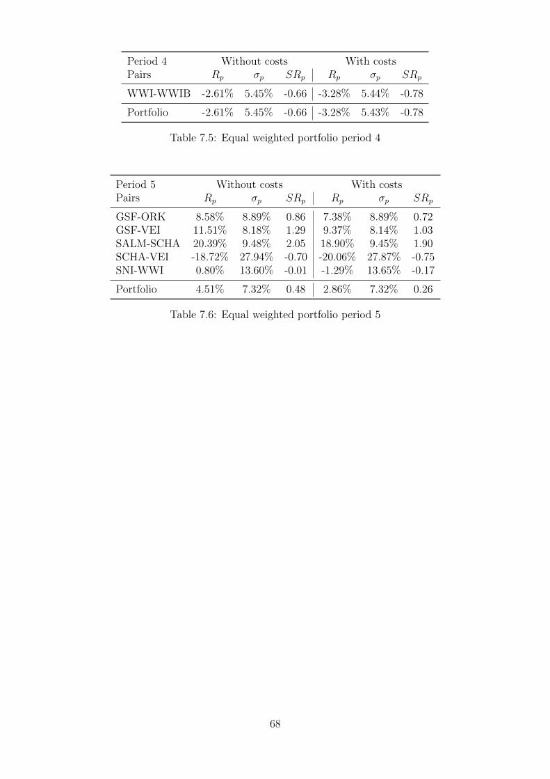
Period 4 Without costs With costsPairs Rp σp SRp Rp σp SRp
WWI-WWIB -2.61% 5.45% -0.66 -3.28% 5.44% -0.78
Portfolio -2.61% 5.45% -0.66 -3.28% 5.43% -0.78
Table 7.5: Equal weighted portfolio period 4
Period 5 Without costs With costsPairs Rp σp SRp Rp σp SRp
GSF-ORK 8.58% 8.89% 0.86 7.38% 8.89% 0.72GSF-VEI 11.51% 8.18% 1.29 9.37% 8.14% 1.03SALM-SCHA 20.39% 9.48% 2.05 18.90% 9.45% 1.90SCHA-VEI -18.72% 27.94% -0.70 -20.06% 27.87% -0.75SNI-WWI 0.80% 13.60% -0.01 -1.29% 13.65% -0.17
Portfolio 4.51% 7.32% 0.48 2.86% 7.32% 0.26
Table 7.6: Equal weighted portfolio period 5
68
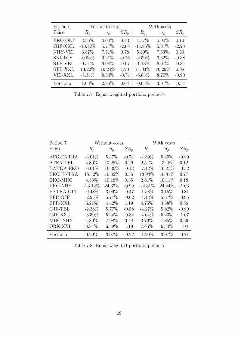
Period 6 Without costs With costsPairs Rp σp SRp Rp σp SRp
EKO-OLT 3.56% 6.00% 0.43 1.57% 5.90% 0.10GJF-XXL -10.72% 5.71% -2.06 -11.96% 5.81% -2.23NHY-VEI 6.87% 7.51% 0.78 5.39% 7.53% 0.59SNI-TGS -0.53% 9.21% -0.16 -2.59% 9.32% -0.38STB-VEI 0.54% 6.08% -0.07 -1.13% 6.07% -0.34STB-XXL 13.22% 10.24% 1.20 11.03% 10.29% 0.98VEI-XXL -5.38% 8.54% -0.74 -6.83% 8.70% -0.90
Portfolio 1.08% 2.96% 0.04 -0.65% 3.01% -0.54
Table 7.7: Equal weighted portfolio period 6
Period 7 Without costs With costsPairs Rp σp SRp Rp σp SRp
AFG-ENTRA -3.01% 5.47% -0.74 -4.39% 5.40% -0.99ATEA-TEL 4.80% 13.25% 0.29 2.51% 13.15% 0.12BAKKA-EKO -6.01% 16.36% -0.43 -7.42% 16.25% -0.52EKO-ENTRA 15.52% 16.82% 0.86 13.93% 16.81% 0.77EKO-MHG 4.53% 10.18% 0.35 2.81% 10.11% 0.18EKO-NHY -23.12% 24.39% -0.99 -24.31% 24.44% -1.03ENTRA-OLT -0.48% 3.09% -0.47 -1.58% 3.15% -0.81EPR-GJF -2.25% 5.71% -0.62 -4.43% 5.67% -0.95EPR-XXL 6.21% 4.42% 1.19 4.75% 4.38% 0.86GJF-TEL -2.38% 5.77% -0.58 -4.27% 5.82% -0.90GJF-XXL -3.30% 5.24% -0.82 -4.64% 5.23% -1.07MHG-NHY 4.80% 7.98% 0.48 3.79% 7.85% 0.36ORK-XXL 8.84% 6.59% 1.19 7.65% 6.44% 1.04
Portfolio 0.29% 3.07% -0.22 -1.20% 3.07% -0.71
Table 7.8: Equal weighted portfolio period 7
69
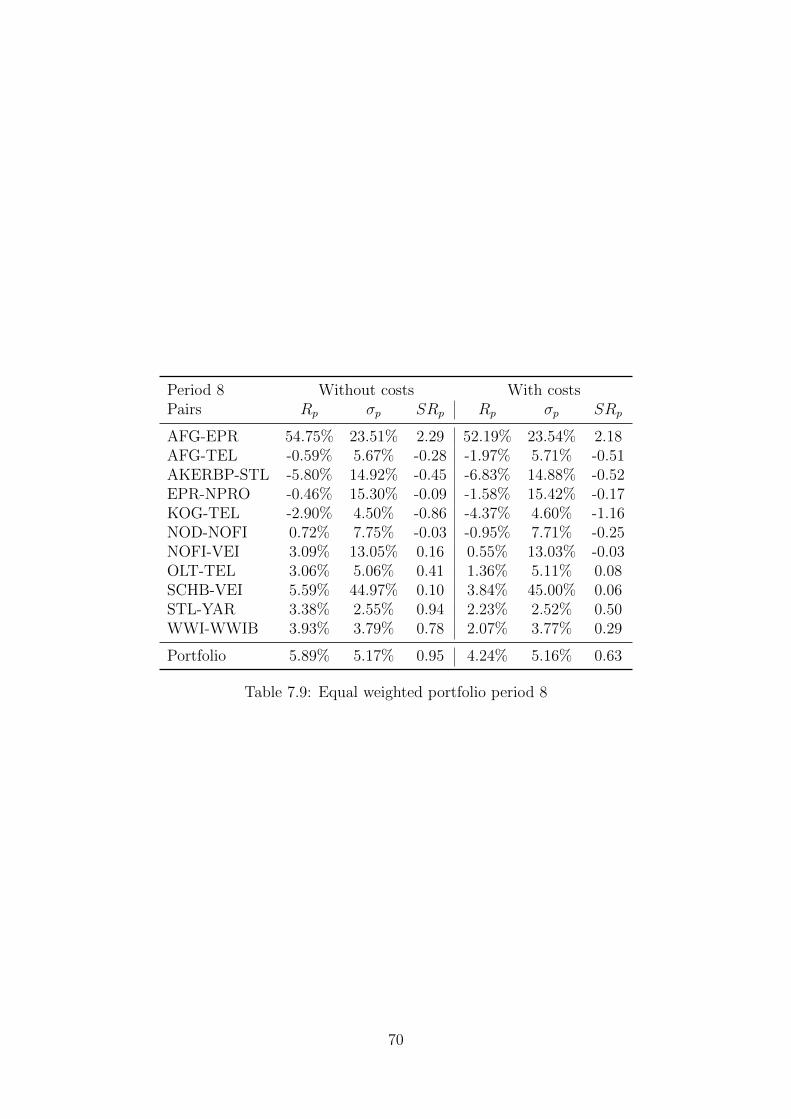
Period 8 Without costs With costsPairs Rp σp SRp Rp σp SRp
AFG-EPR 54.75% 23.51% 2.29 52.19% 23.54% 2.18AFG-TEL -0.59% 5.67% -0.28 -1.97% 5.71% -0.51AKERBP-STL -5.80% 14.92% -0.45 -6.83% 14.88% -0.52EPR-NPRO -0.46% 15.30% -0.09 -1.58% 15.42% -0.17KOG-TEL -2.90% 4.50% -0.86 -4.37% 4.60% -1.16NOD-NOFI 0.72% 7.75% -0.03 -0.95% 7.71% -0.25NOFI-VEI 3.09% 13.05% 0.16 0.55% 13.03% -0.03OLT-TEL 3.06% 5.06% 0.41 1.36% 5.11% 0.08SCHB-VEI 5.59% 44.97% 0.10 3.84% 45.00% 0.06STL-YAR 3.38% 2.55% 0.94 2.23% 2.52% 0.50WWI-WWIB 3.93% 3.79% 0.78 2.07% 3.77% 0.29
Portfolio 5.89% 5.17% 0.95 4.24% 5.16% 0.63
Table 7.9: Equal weighted portfolio period 8
70
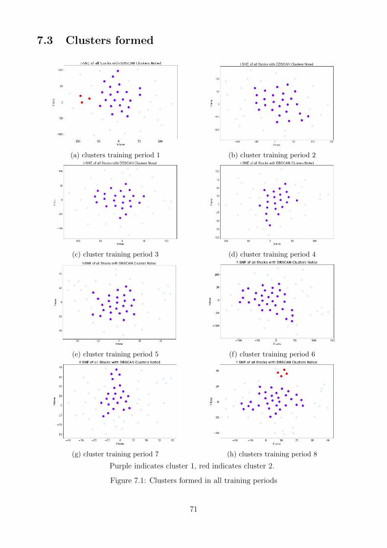
7.3 Clusters formed
(a) clusters training period 1 (b) cluster training period 2
(c) cluster training period 3 (d) cluster training period 4
(e) cluster training period 5 (f) cluster training period 6
(g) cluster training period 7 (h) clusters training period 8
Purple indicates cluster 1, red indicates cluster 2.
Figure 7.1: Clusters formed in all training periods
71
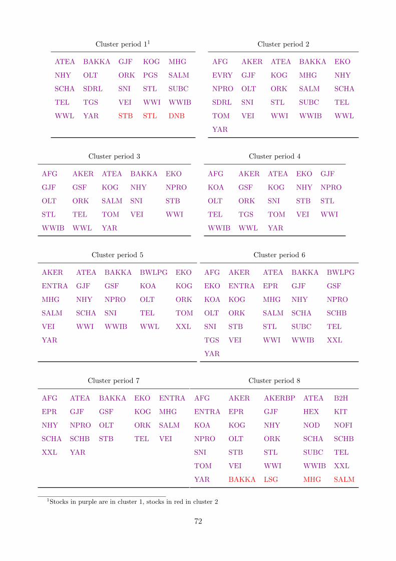
Cluster period 11
ATEA BAKKA GJF KOG MHG
NHY OLT ORK PGS SALM
SCHA SDRL SNI STL SUBC
TEL TGS VEI WWI WWIB
WWL YAR STB STL DNB
Cluster period 2
AFG AKER ATEA BAKKA EKO
EVRY GJF KOG MHG NHY
NPRO OLT ORK SALM SCHA
SDRL SNI STL SUBC TEL
TOM VEI WWI WWIB WWL
YAR
Cluster period 3
AFG AKER ATEA BAKKA EKO
GJF GSF KOG NHY NPRO
OLT ORK SALM SNI STB
STL TEL TOM VEI WWI
WWIB WWL YAR
Cluster period 4
AFG AKER ATEA EKO GJF
KOA GSF KOG NHY NPRO
OLT ORK SNI STB STL
TEL TGS TOM VEI WWI
WWIB WWL YAR
Cluster period 5
AKER ATEA BAKKA BWLPG EKO
ENTRA GJF GSF KOA KOG
MHG NHY NPRO OLT ORK
SALM SCHA SNI TEL TOM
VEI WWI WWIB WWL XXL
YAR
Cluster period 6
AFG AKER ATEA BAKKA BWLPG
EKO ENTRA EPR GJF GSF
KOA KOG MHG NHY NPRO
OLT ORK SALM SCHA SCHB
SNI STB STL SUBC TEL
TGS VEI WWI WWIB XXL
YAR
Cluster period 7
AFG ATEA BAKKA EKO ENTRA
EPR GJF GSF KOG MHG
NHY NPRO OLT ORK SALM
SCHA SCHB STB TEL VEI
XXL YAR
Cluster period 8
AFG AKER AKERBP ATEA B2H
ENTRA EPR GJF HEX KIT
KOA KOG NHY NOD NOFI
NPRO OLT ORK SCHA SCHB
SNI STB STL SUBC TEL
TOM VEI WWI WWIB XXL
YAR BAKKA LSG MHG SALM
1Stocks in purple are in cluster 1, stocks in red in cluster 2
72
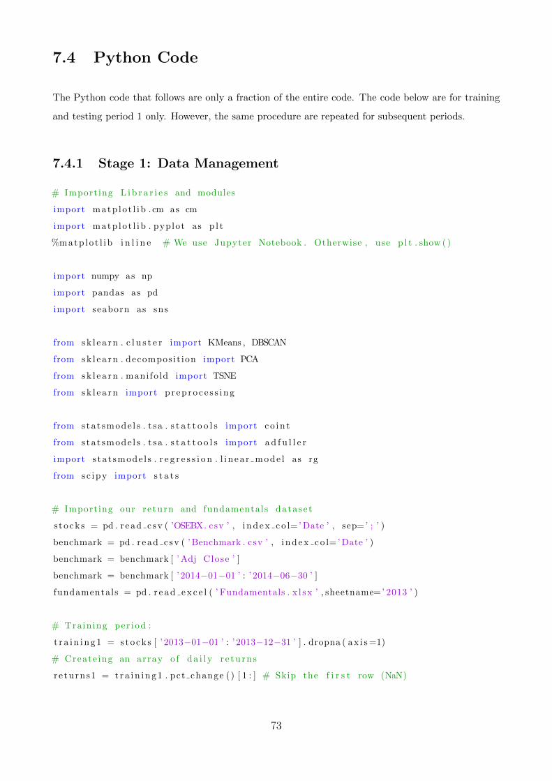
7.4 Python Code
The Python code that follows are only a fraction of the entire code. The code below are for training
and testing period 1 only. However, the same procedure are repeated for subsequent periods.
7.4.1 Stage 1: Data Management
# Importing L i b r a r i e s and modules
import matp lo t l i b . cm as cm
import matp lo t l i b . pyplot as p l t
%matp lo t l i b i n l i n e # We use Jupyter Notebook . Otherwise , use p l t . show ( )
import numpy as np
import pandas as pd
import seaborn as sns
from s k l ea rn . c l u s t e r import KMeans , DBSCAN
from s k l ea rn . decomposit ion import PCA
from s k l ea rn . mani fo ld import TSNE
from s k l ea rn import p r e p r o c e s s i n g
from stat smode l s . t sa . s t a t t o o l s import c o i n t
from stat smode l s . t sa . s t a t t o o l s import a d f u l l e r
import s ta t smode l s . r e g r e s s i o n . l i n ea r mode l as rg
from sc ipy import s t a t s
# Importing our re turn and fundamentals datase t
s t o ck s = pd . r ead c sv ( ’OSEBX. csv ’ , i n d e x c o l=’ Date ’ , sep=’ ; ’ )
benchmark = pd . r ead c sv ( ’ Benchmark . csv ’ , i n d e x c o l=’ Date ’ )
benchmark = benchmark [ ’ Adj Close ’ ]
benchmark = benchmark [ ’ 2014−01−01 ’ : ’ 2014−06−30 ’ ]
fundamentals = pd . r e a d e x c e l ( ’ Fundamentals . x l sx ’ , sheetname=’ 2013 ’ )
# Training per iod :
t r a i n i n g 1 = s tock s [ ’ 2013−01−01 ’ : ’ 2013−12−31 ’ ] . dropna ( a x i s =1)
# Create ing an array o f d a i l y r e tu rn s
r e turns1 = t r a i n i n g 1 . pct change ( ) [ 1 : ] # Skip the f i r s t row (NaN)
73
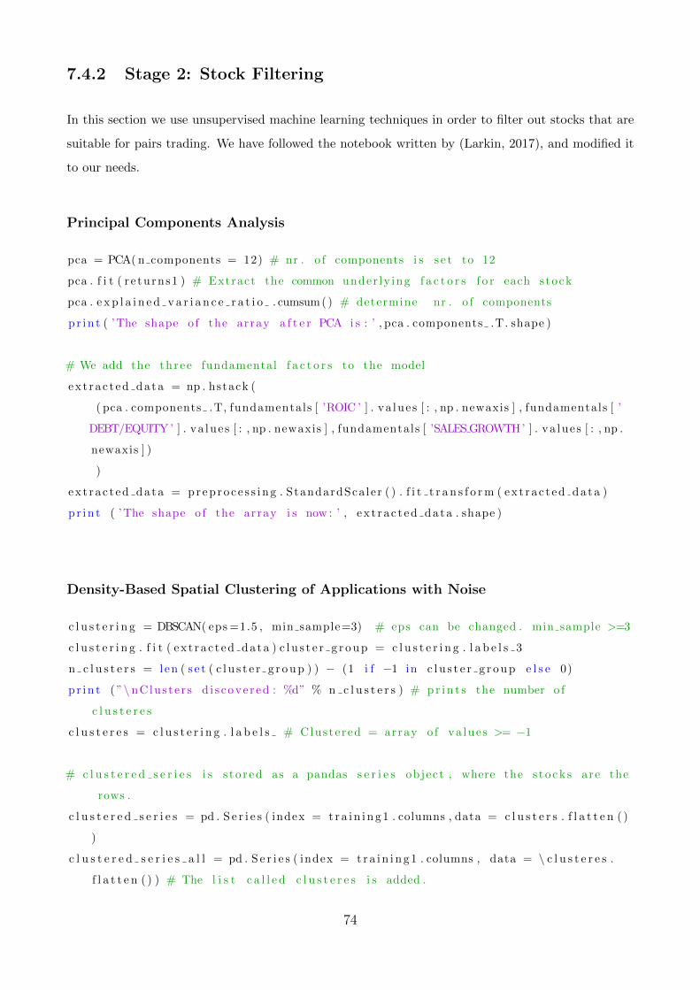
7.4.2 Stage 2: Stock Filtering
In this section we use unsupervised machine learning techniques in order to filter out stocks that are
suitable for pairs trading. We have followed the notebook written by (Larkin, 2017), and modified it
to our needs.
Principal Components Analysis
pca = PCA( n components = 12) # nr . o f components i s s e t to 12
pca . f i t ( r e turns1 ) # Extract the common under ly ing f a c t o r s f o r each stock
pca . e x p l a i n e d v a r i a n c e r a t i o . cumsum( ) # determine nr . o f components
p r i n t ( ’The shape o f the array a f t e r PCA i s : ’ , pca . components .T. shape )
# We add the three fundamental f a c t o r s to the model
ex t rac t ed data = np . hstack (
( pca . components .T, fundamentals [ ’ROIC ’ ] . va lue s [ : , np . newaxis ] , fundamentals [ ’
DEBT/EQUITY ’ ] . va lue s [ : , np . newaxis ] , fundamentals [ ’SALES GROWTH’ ] . va lue s [ : , np .
newaxis ] )
)
ex t rac t ed data = p r e p r o c e s s i n g . StandardSca ler ( ) . f i t t r a n s f o r m ( ex t rac t ed data )
p r i n t ( ’The shape o f the array i s now : ’ , ex t rac t ed data . shape )
Density-Based Spatial Clustering of Applications with Noise
c l u s t e r i n g = DBSCAN( eps =1.5 , min sample=3) # eps can be changed . min sample >=3
c l u s t e r i n g . f i t ( ex t rac t ed data ) c l u s t e r g r o u p = c l u s t e r i n g . l a b e l s 3
n c l u s t e r s = len ( s e t ( c l u s t e r g r o u p ) ) − (1 i f −1 in c l u s t e r g r o u p e l s e 0)
p r i n t ( ”\ nClus te r s d i s cove r ed : %d” % n c l u s t e r s ) # p r i n t s the number o f
c l u s t e r e s
c l u s t e r e s = c l u s t e r i n g . l a b e l s # Clustered = array o f va lue s >= −1
# c l u s t e r e d s e r i e s i s s to r ed as a pandas s e r i e s object , where the s to ck s are the
rows .
c l u s t e r e d s e r i e s = pd . S e r i e s ( index = t r a i n i n g 1 . columns , data = c l u s t e r s . f l a t t e n ( )
)
c l u s t e r e d s e r i e s a l l = pd . S e r i e s ( index = t r a i n i n g 1 . columns , data = \ c l u s t e r e s .
f l a t t e n ( ) ) # The l i s t c a l l e d c l u s t e r e s i s added .
74
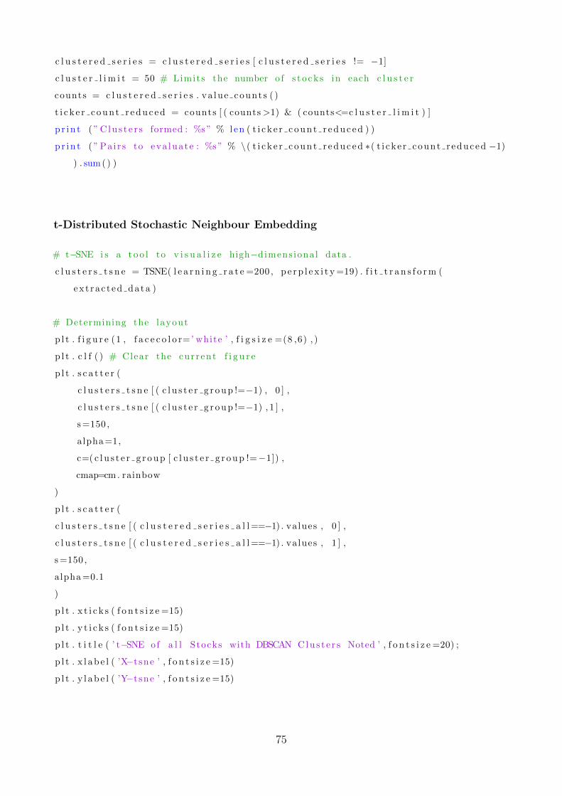
c l u s t e r e d s e r i e s = c l u s t e r e d s e r i e s [ c l u s t e r e d s e r i e s != −1]
c l u s t e r l i m i t = 50 # Limits the number o f s t o ck s in each c l u s t e r
counts = c l u s t e r e d s e r i e s . va lue count s ( )
t i c k e r c o u n t r e d u c e d = counts [ ( counts>1) & ( counts<=c l u s t e r l i m i t ) ]
p r i n t ( ” C lu s t e r s formed : %s ” % len ( t i c k e r c o u n t r e d u c e d ) )
p r i n t ( ” Pa i r s to eva luate : %s ” % \( t i c k e r c o u n t r e d u c e d ∗( t i cke r count r educed −1)
) . sum ( ) )
t-Distributed Stochastic Neighbour Embedding
# t−SNE i s a t o o l to v i s u a l i z e high−dimens iona l data .
c l u s t e r s t s n e = TSNE( l e a r n i n g r a t e =200 , p e r p l e x i t y =19) . f i t t r a n s f o r m (
ex t rac t ed data )
# Determining the layout
p l t . f i g u r e (1 , f a c e c o l o r=’ white ’ , f i g s i z e =(8 ,6) , )
p l t . c l f ( ) # Clear the cur rent f i g u r e
p l t . s c a t t e r (
c l u s t e r s t s n e [ ( c l u s t e r g r o u p !=−1) , 0 ] ,
c l u s t e r s t s n e [ ( c l u s t e r g r o u p !=−1) , 1 ] ,
s =150 ,
alpha =1,
c=( c l u s t e r g r o u p [ c l u s t e r g r o u p !=−1]) ,
cmap=cm. rainbow
)
p l t . s c a t t e r (
c l u s t e r s t s n e [ ( c l u s t e r e d s e r i e s a l l ==−1) . values , 0 ] ,
c l u s t e r s t s n e [ ( c l u s t e r e d s e r i e s a l l ==−1) . values , 1 ] ,
s =150 ,
alpha =0.1
)
p l t . x t i c k s ( f o n t s i z e =15)
p l t . y t i c k s ( f o n t s i z e =15)
p l t . t i t l e ( ’ t−SNE of a l l Stocks with DBSCAN Clus t e r s Noted ’ , f o n t s i z e =20) ;
p l t . x l a b e l ( ’X−t sne ’ , f o n t s i z e =15)
p l t . y l a b e l ( ’Y−t sne ’ , f o n t s i z e =15)
75
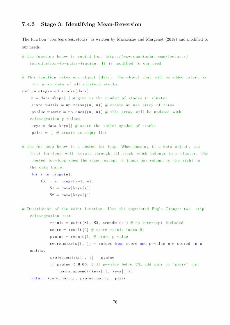
7.4.3 Stage 3: Identifying Mean-Reversion
The function ”cointegrated−stocks” is written by Mackenzie and Margenot (2018) and modified to
our needs.
# The func t i on below i s copied from https : //www. quantopian . com/ l e c t u r e s /
in t roduct i on−to−pa i r s−t rad ing . I t i s modi f i ed to our need
# This func t i on takes one ob j e c t ( data ) . The ob j e c t that w i l l be added l a t e r , i s
the p r i c e data o f a l l c l u s t e r d s to ck s .
de f c o i n t e g r a t e d s t o c k s ( data ) :
n = data . shape [ 1 ] # g ive us the number o f s t o ck s in c l u s t e r
s co r e mat r i x = np . z e ro s ( ( n , n) ) # c r e a t e an n∗n array o f z e r o s
pva lue matr ix = np . ones ( ( n , n) ) # t h i s array w i l l be updated with
c o i n t e g r a t i o n p−va lue s
keys = data . keys ( ) # s t o r e the t i c k e r symbol o f s t o ck s
p a i r s = [ ] # c r e a t e an empty l i s t
# The f o r loop below i s a nested for−loop . When pass ing in a data object , the
f i r s t for−loop w i l l i t e r a t e through a l l s tock which be longs to a c l u s t e r . The
nested for−loop does the same , except i t jumps one column to the r i g h t in
the data frame .
f o r i in range (n) :
f o r j in range ( i +1, n) :
S1 = data [ keys [ i ] ]
S2 = data [ keys [ j ] ]
# Desc r ip t i on o f the c o i n t func t i on : Uses the augmented Engle−Granger two− s tep
c o i n t e g r a t i o n t e s t .
r e s u l t = co i n t ( S1 , S2 , trend=’ nc ’ ) # no i n t e r c e p t inc luded .
s co r e = r e s u l t [ 0 ] # s t o r e r e s u l t index [ 0 ]
pvalue = r e s u l t [ 1 ] # s t o r e p−value
s co r e mat r i x [ i , j ] = va lue s from sco r e and p−value are s to r ed in a
matrix .
pva lue matr ix [ i , j ] = pvalue
i f pvalue < 0 . 0 5 : # I f p−value below 5%, add pa i r to ” p a i r s ” l i s t
p a i r s . append ( ( keys [ i ] , keys [ j ] ) )
r e turn score matr ix , pvalue matr ix , p a i r s
76
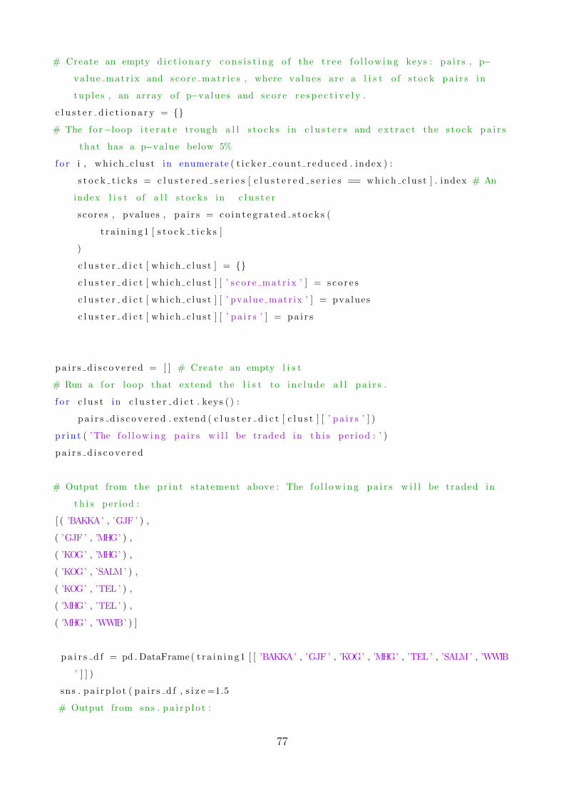
# Create an empty d i c t i o n a r y c o n s i s t i n g o f the t r e e f o l l o w i n g keys : pa i r s , p−
va lue matr ix and sco r e mat r i c s , where va lue s are a l i s t o f s tock p a i r s in
tup le s , an array o f p−va lue s and s co r e r e s p e c t i v e l y .
c l u s t e r d i c t i o n a r y =
# The for−loop i t e r a t e trough a l l s t o ck s in c l u s t e r s and e x t r a c t the s tock p a i r s
that has a p−value below 5%
f o r i , wh i ch c lu s t in enumerate ( t i c k e r c o u n t r e d u c e d . index ) :
s t o c k t i c k s = c l u s t e r e d s e r i e s [ c l u s t e r e d s e r i e s == whi ch c lu s t ] . index # An
index l i s t o f a l l s t o ck s in c l u s t e r
s co re s , pvalues , p a i r s = c o i n t e g r a t e d s t o c k s (
t r a i n i n g 1 [ s t o c k t i c k s ]
)
c l u s t e r d i c t [ wh i ch c lu s t ] =
c l u s t e r d i c t [ wh i ch c lu s t ] [ ’ s co r e mat r i x ’ ] = s c o r e s
c l u s t e r d i c t [ wh i ch c lu s t ] [ ’ pva lue matr ix ’ ] = pvalues
c l u s t e r d i c t [ wh i ch c lu s t ] [ ’ p a i r s ’ ] = p a i r s
p a i r s d i s c o v e r e d = [ ] # Create an empty l i s t
# Run a f o r loop that extend the l i s t to in c lude a l l p a i r s .
f o r c l u s t in c l u s t e r d i c t . keys ( ) :
p a i r s d i s c o v e r e d . extend ( c l u s t e r d i c t [ c l u s t ] [ ’ p a i r s ’ ] )
p r i n t ( ’The f o l l o w i n g p a i r s w i l l be traded in t h i s per iod : ’ )
p a i r s d i s c o v e r e d
# Output from the p r in t statement above : The f o l l o w i n g p a i r s w i l l be traded in
t h i s per iod :
[ ( ’BAKKA’ , ’GJF ’ ) ,
( ’GJF ’ , ’MHG’ ) ,
( ’KOG’ , ’MHG’ ) ,
( ’KOG’ , ’SALM’ ) ,
( ’KOG’ , ’TEL ’ ) ,
( ’MHG’ , ’TEL ’ ) ,
( ’MHG’ , ’WWIB’ ) ]
p a i r s d f = pd . DataFrame ( t r a i n i n g 1 [ [ ’BAKKA’ , ’GJF ’ , ’KOG’ , ’MHG’ , ’TEL ’ , ’SALM’ , ’WWIB
’ ] ] )
sns . p a i r p l o t ( p a i r s d f , s i z e =1.5
# Output from sns . p a i r p l o t :
77
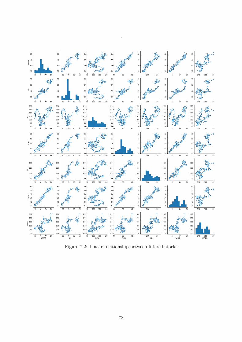
.
Figure 7.2: Linear relationship between filtered stocks
78
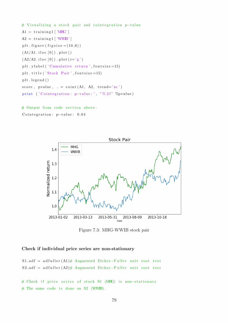
# V i s u a l i z i n g a stock pa i r and c o i n t e g r a t i o n p−value
A1 = t r a i n i n g 1 [ ’MHG’ ]
A2 = t r a i n i n g 1 [ ’WWIB’ ]
p l t . f i g u r e ( f i g s i z e =(10 ,6) )
(A1/A1 . i l o c [ 0 ] ) . p l o t ( )
(A2/A2 . i l o c [ 0 ] ) . p l o t ( c=’ g ’ )
p l t . y l a b e l ( ’ Cumulative re turn ’ , f o n t s i z e =15)
p l t . t i t l e ( ’ Stock Pair ’ , f o n t s i z e =15)
p l t . l egend ( )
score , pvalue , = c o i n t (A1 , A2 , trend=’ nc ’ )
p r i n t ( ’ Co integrat i on : p−value : ’ , ”%.2 f ” %pvalue )
# Output from code s e c t i o n above :
Co integrat i on : p−value : 0 .04
Figure 7.3: MHG-WWIB stock pair
Check if individual price series are non-stationary
S1 adf = a d f u l l e r (A1)# Augmented Dickey−F u l l e r un i t root t e s t
S2 adf = a d f u l l e r (A2)# Augmented Dickey−F u l l e r un i t root t e s t
# Check i f p r i c e s e r i e s o f s tock S1 (MHG) i s non−s t a t i o n a r y
# The same code i s done on S2 (WWIB) .
79
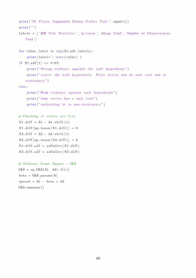
pr in t ( ”S1 Pr i c e s Augmented Dickey−F u l l e r Test : ” . upper ( ) )
p r i n t ( ”” )
l a b e l s = [ ’ADF Test S t a t i s t i c ’ , ’p−value ’ , ’#Lags Used ’ , ’Number o f Observat ions
Used ’ ]
f o r value , l a b e l in z ip ( S1 adf , l a b e l s ) :
p r i n t ( l a b e l+’ : ’+s t r ( va lue ) )
i f S1 adf [ 1 ] <= 0 . 0 5 :
p r i n t ( ” Strong ev idence aga in s t the n u l l hypothes i s ” )
p r i n t ( ” r e j e c t the n u l l hypothes i s . Pr i ce s e r i e s has no un i t root and i s
s t a t i o n a r y ” )
e l s e :
p r i n t ( ”Weak ev idence aga in s t n u l l hypothes i s ” )
p r i n t ( ” time s e r i e s has a un i t root ” )
p r i n t ( ” i n d i c a t i n g i t i s non−s t a t i o n a r y ” )
# Checking i f s e r i e s are I (1 )
S 1 d i f f = A1 − A1 . s h i f t (1 )
S 1 d i f f [ np . i snan ( S 1 d i f f ) ] = 0
S 2 d i f f = A2 − A2 . s h i f t (1 )
S 2 d i f f [ np . i snan ( S 2 d i f f ) ] = 0
S 1 d i f f a d f = a d f u l l e r ( S 1 d i f f )
S 2 d i f f a d f = a d f u l l e r ( S 2 d i f f )
# Ordinary Least Square − OLS
OLS = rg .OLS(A1 , A2) . f i t ( )
beta = OLS. params [ 0 ]
spread = A1 − beta ∗ A2
OLS. summary ( )
80
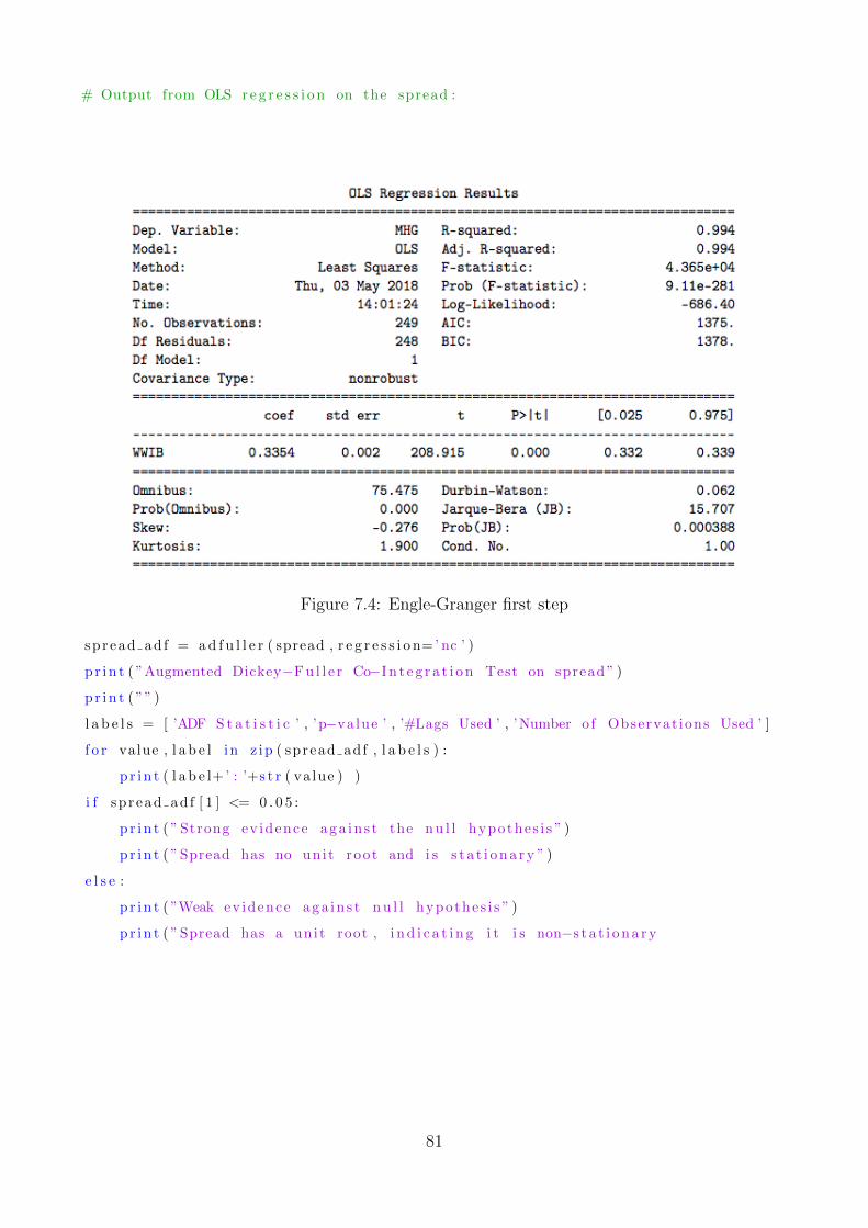
# Output from OLS r e g r e s s i o n on the spread :
Figure 7.4: Engle-Granger first step
spread ad f = a d f u l l e r ( spread , r e g r e s s i o n=’ nc ’ )
p r i n t ( ”Augmented Dickey−F u l l e r Co−I n t e g r a t i o n Test on spread ” )
p r i n t ( ”” )
l a b e l s = [ ’ADF S t a t i s t i c ’ , ’p−value ’ , ’#Lags Used ’ , ’Number o f Observat ions Used ’ ]
f o r value , l a b e l in z ip ( spread adf , l a b e l s ) :
p r i n t ( l a b e l+’ : ’+s t r ( va lue ) )
i f sp r ead ad f [ 1 ] <= 0 . 0 5 :
p r i n t ( ” Strong ev idence aga in s t the n u l l hypothes i s ” )
p r i n t ( ”Spread has no un i t root and i s s t a t i o n a r y ” )
e l s e :
p r i n t ( ”Weak ev idence aga in s t n u l l hypothes i s ” )
p r i n t ( ”Spread has a un i t root , i n d i c a t i n g i t i s non−s t a t i o n a r y
81
Augmented Dickey-Fuller Test on spread
ADF Statistic: -2.06360186303
p-value: 0.037411835533
Lags Used : 0
Number of Observations Used: 248
Strong evidence against the null hypothesis, spread has no unit root and is stationary
7.4.4 Stage 4: Trading Setup and Execution
In this section the trading algorithm is created. The steps in the trading setup are done for all stock
pairs.
# S l i c i n g out f i r s t t e s t i n g per iod and a pa i r that are c o i n t e g r a t e d .
pa i r1 = s tock s . l o c [ ’ 2014−01−01 ’ : ’ 2014−06−30 ’ , [ ’MHG’ , ’WWIB’ ] ] . dropna ( )
pa i r1 . columns = [ ’ S1 ’ , ’ S2 ’ ]
# Creat ing re turn columns f o r each stock in pa i r1
pa i r1 [ ’ S1ret ’ ] = pa i r1 [ ’ S1 ’ ] . pct change (1 )
pa i r1 . i l o c [ 0 , 2 ] = 0
pa i r1 [ ’ S2ret ’ ] = pa i r1 [ ’ S2 ’ ] . pct change (1 )
pa i r1 . i l o c [ 0 , 3 ] = 0
Creating the rolling z-score
# OLS − Regres s ion
lm pai r1 = rg .OLS( pa i r1 [ ’ S1 ’ ] , pa i r1 [ ’ S2 ’ ] ) . f i t ( )
pa i r1 b1 = lm pai r1 . params [ 0 ]
# Creat ing a new column c a l l e s ’ p a i r s p r e a d ’
pa i r1 [ ’ p a i r s p r e a d ’ ] = pa i r1 [ ’ S1 ’ ] − pa i r1 b1 ∗ pa i r1 [ ’ S2 ’ ]
# Ca l cu l a t i on the r o l l i n g 10−day covar iance
r o l l i n g p a i r c o v = pa i r1 . l o c [ : , [ ’ S1 ’ , ’ S2 ’ ] ] . \
r o l l i n g ( window=10) . cov ( pa i r1 . l o c [ : , [ ’ S1 ’ , ’ S2 ’ ] ] , pa i rw i s e=True )
82

# S l i c e mult i index dataframe to s i n g l e index dataframe o f pa i r ed s tock s
covar iance
idx = pd . I n d e x S l i c e
r o l l i n g p a i r c o v = r o l l i n g p a i r c o v . l o c [ idx [ : , ’ S1 ’ ] , ’ S2 ’ ]
# Converting Date and stock index in to date index , by making stock at index
l e v e l 1 in to a new column
r o l l i n g p a i r c o v = r o l l i n g p a i r c o v . r e s e t i n d e x ( l e v e l =1)
# Ca l cu l a t ing the 10−day r o l l i n g var iance
r o l l i n g p a i r v a r = pa i r1 [ ’ S2 ’ ] . r o l l i n g ( window=10) . var ( )
# ROLLING BETA
pa i r1 [ ’ r o l l i n g p a i r b 1 ’ ] = r o l l i n g p a i r c o v [ ’ S2 ’ ] / r o l l i n g p a i r v a r
# CALCULATION OF THE 10−DAY ROLLING SPREAD:
pa i r1 [ ’ r o l l i n g p a i r s p r e a d ’ ] = pa i r1 [ ’ S1 ’ ] − pa i r1 [ ’ r o l l i n g p a i r b 1 ’ ] ∗ pa i r1 [ ’
S2 ’ ]
10-day rolling z-score
# CALCULATION OF THE 10−DAY ROLLING Z−SCORE:
pa i r1 [ ’ r o l l i n g Z s c o r e ’ ] = ( pa i r1 [ ’ r o l l i n g p a i r s p r e a d ’ ] − \
pa i r1 [ ’ r o l l i n g p a i r s p r e a d ’ ] . r o l l i n g ( window=10) . mean
( ) ) / \
pa i r1 [ ’ r o l l i n g p a i r s p r e a d ’ ] . r o l l i n g ( window=10) . s td
( )
83
Trading Signals Algorithm
# TRADING SIGNALS ALGORITHM
# Z−s co r e the day be f o r e
pa i r1 [ ’ r o l l i n g Z s c o r e (−1) ’ ] = pa i r1 [ ’ r o l l i n g Z s c o r e ’ ] . s h i f t (1 )
# Z−s co r e two days be f o r e
pa i r1 [ ’ r o l l i n g Z s c o r e (−2) ’ ] = pa i r1 [ ’ r o l l i n g Z s c o r e ’ ] . s h i f t (2 )
pa i r1 [ ’ p a i r s i g n a l ’ ] = 0
p a i r s i g n a l = 0
# The for−loop below i s exp la ined in s e c t i o n 3.5.1−Trading s i g n a l s and execut ion
f o r i , r in enumerate ( pa i r1 . i t e r r o w s ( ) ) :
i f r [ 1 ] [ ’ r o l l i n g Z s c o r e (−2) ’ ] > −2 and r [ 1 ] [ ’ r o l l i n g Z s c o r e (−1) ’ ] < −2:
p a i r s i g n a l = −2
e l i f r [ 1 ] [ ’ r o l l i n g Z s c o r e (−2) ’ ] < −1 and r [ 1 ] [ ’ r o l l i n g Z s c o r e (−1) ’ ] > −1:
p a i r s i g n a l = −1
e l i f r [ 1 ] [ ’ r o l l i n g Z s c o r e (−2) ’ ] < 2 and r [ 1 ] [ ’ r o l l i n g Z s c o r e (−1) ’ ] > 2 :
p a i r s i g n a l = 2
e l i f r [ 1 ] [ ’ r o l l i n g Z s c o r e (−2) ’ ] > 1 and r [ 1 ] [ ’ r o l l i n g Z s c o r e (−1) ’ ] < 1 :
p a i r s i g n a l = 1
e l s e :
p a i r s i g n a l = 0
pa i r1 . i l o c [ i , 10 ] = p a i r s i g n a l
# TRADING POSITIONS : 1 = LONG SPREAD TRADE, −1 = SHORT SPREAD TRADE
pa i r1 [ ’ p o s i t i o n ’ ] = 0
p o s i t i o n = 0
f o r i , r in enumerate ( pa i r1 . i t e r r o w s ( ) ) :
i f r [ 1 ] [ ’ p a i r s i g n a l ’ ] == −2:
p o s i t i o n = 1
e l i f r [ 1 ] [ ’ p a i r s i g n a l ’ ] == −1:
p o s i t i o n = 0
e l i f r [ 1 ] [ ’ p a i r s i g n a l ’ ] == 2 :
p o s i t i o n = −1
e l i f r [ 1 ] [ ’ p a i r s i g n a l ’ ] == 1 :
p o s i t i o n = 0
e l s e :
p o s i t i o n = pa i r1 . l o c [ : , ’ p o s i t i o n ’ ] [ i −1]
pa i r1 . i l o c [ i , 11 ] = p o s i t i o n
84
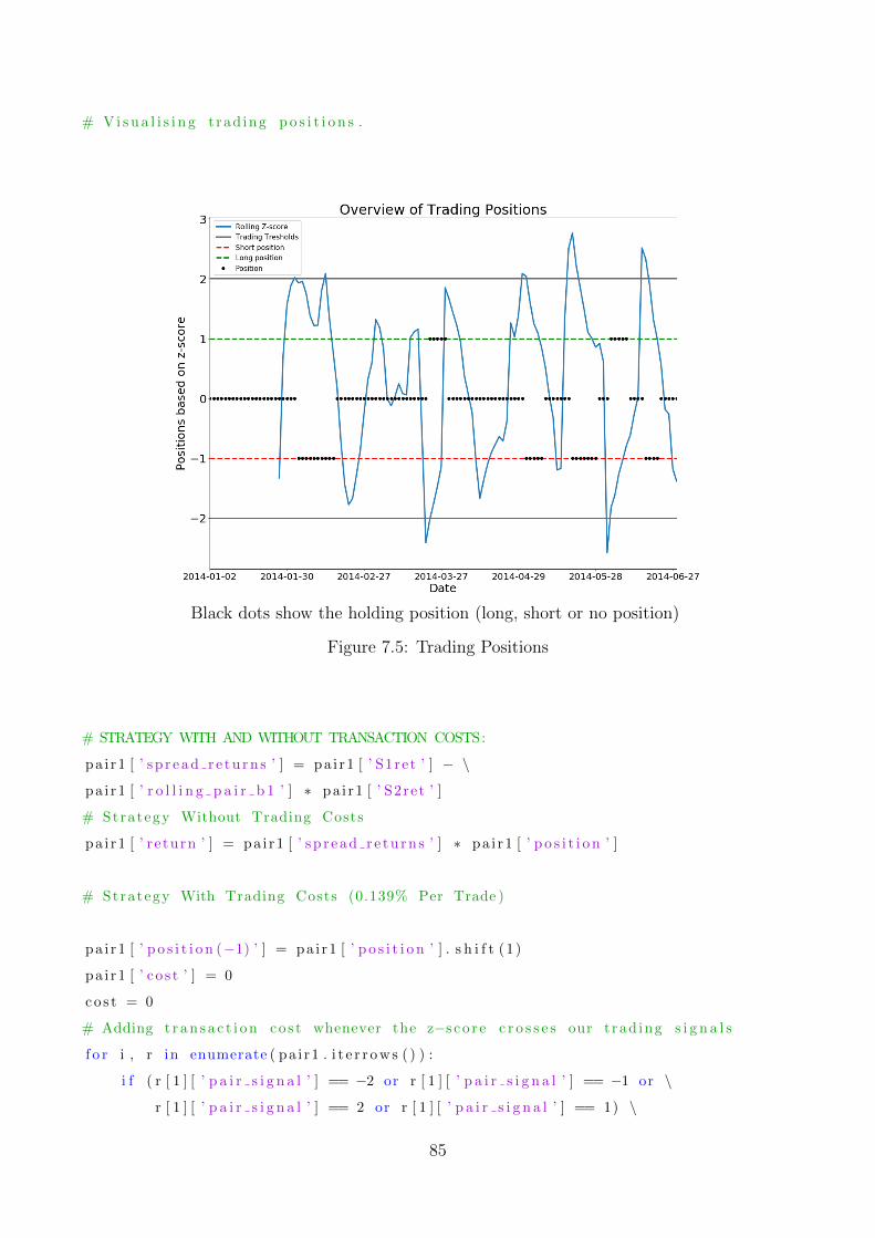
# V i s u a l i s i n g t rad ing p o s i t i o n s .
Black dots show the holding position (long, short or no position)
Figure 7.5: Trading Positions
# STRATEGY WITH AND WITHOUT TRANSACTION COSTS:
pa i r1 [ ’ s p r ea d r e tu rn s ’ ] = pa i r1 [ ’ S1ret ’ ] − \
pa i r1 [ ’ r o l l i n g p a i r b 1 ’ ] ∗ pa i r1 [ ’ S2ret ’ ]
# Strategy Without Trading Costs
pa i r1 [ ’ r e turn ’ ] = pa i r1 [ ’ s p r ea d r e tu rn s ’ ] ∗ pa i r1 [ ’ p o s i t i o n ’ ]
# Strategy With Trading Costs (0.139% Per Trade )
pa i r1 [ ’ p o s i t i o n (−1) ’ ] = pa i r1 [ ’ p o s i t i o n ’ ] . s h i f t (1 )
pa i r1 [ ’ c o s t ’ ] = 0
co s t = 0
# Adding t r a n s a c t i o n co s t whenever the z−s co r e c r o s s e s our t rad ing s i g n a l s
f o r i , r in enumerate ( pa i r1 . i t e r r o w s ( ) ) :
i f ( r [ 1 ] [ ’ p a i r s i g n a l ’ ] == −2 or r [ 1 ] [ ’ p a i r s i g n a l ’ ] == −1 or \
r [ 1 ] [ ’ p a i r s i g n a l ’ ] == 2 or r [ 1 ] [ ’ p a i r s i g n a l ’ ] == 1) \
85
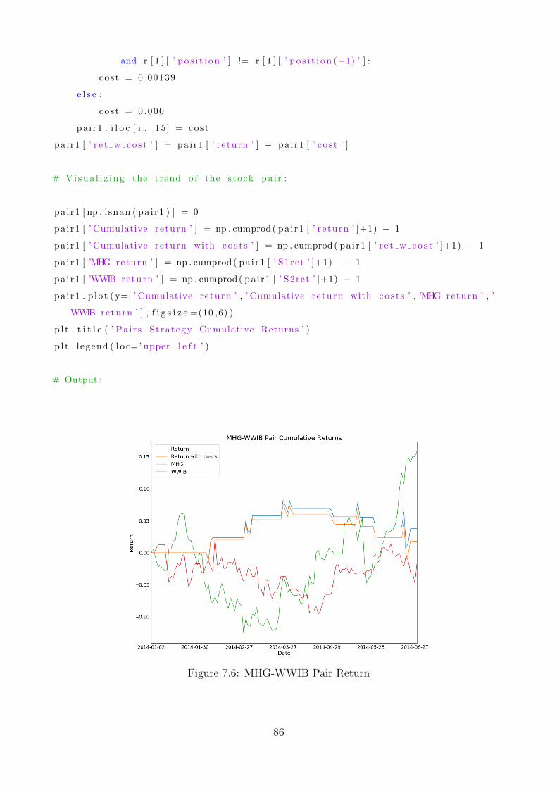
and r [ 1 ] [ ’ p o s i t i o n ’ ] != r [ 1 ] [ ’ p o s i t i o n (−1) ’ ] :
c o s t = 0.00139
e l s e :
co s t = 0.000
pa i r1 . i l o c [ i , 15 ] = co s t
pa i r1 [ ’ r e t w c o s t ’ ] = pa i r1 [ ’ r e turn ’ ] − pa i r1 [ ’ c o s t ’ ]
# V i s u a l i z i n g the trend o f the s tock pa i r :
pa i r1 [ np . i snan ( pa i r1 ) ] = 0
pa i r1 [ ’ Cumulative re turn ’ ] = np . cumprod ( pa i r1 [ ’ r e turn ’ ]+1) − 1
pa i r1 [ ’ Cumulative re turn with c o s t s ’ ] = np . cumprod ( pa i r1 [ ’ r e t w c o s t ’ ]+1) − 1
pa i r1 [ ’MHG return ’ ] = np . cumprod ( pa i r1 [ ’ S1ret ’ ]+1) − 1
pa i r1 [ ’WWIB return ’ ] = np . cumprod ( pa i r1 [ ’ S2ret ’ ]+1) − 1
pa i r1 . p l o t ( y=[ ’ Cumulative re turn ’ , ’ Cumulative re turn with c o s t s ’ , ’MHG return ’ , ’
WWIB return ’ ] , f i g s i z e =(10 ,6) )
p l t . t i t l e ( ’ Pa i r s Strategy Cumulative Returns ’ )
p l t . l egend ( l o c=’ upper l e f t ’ )
# Output :
Figure 7.6: MHG-WWIB Pair Return
86
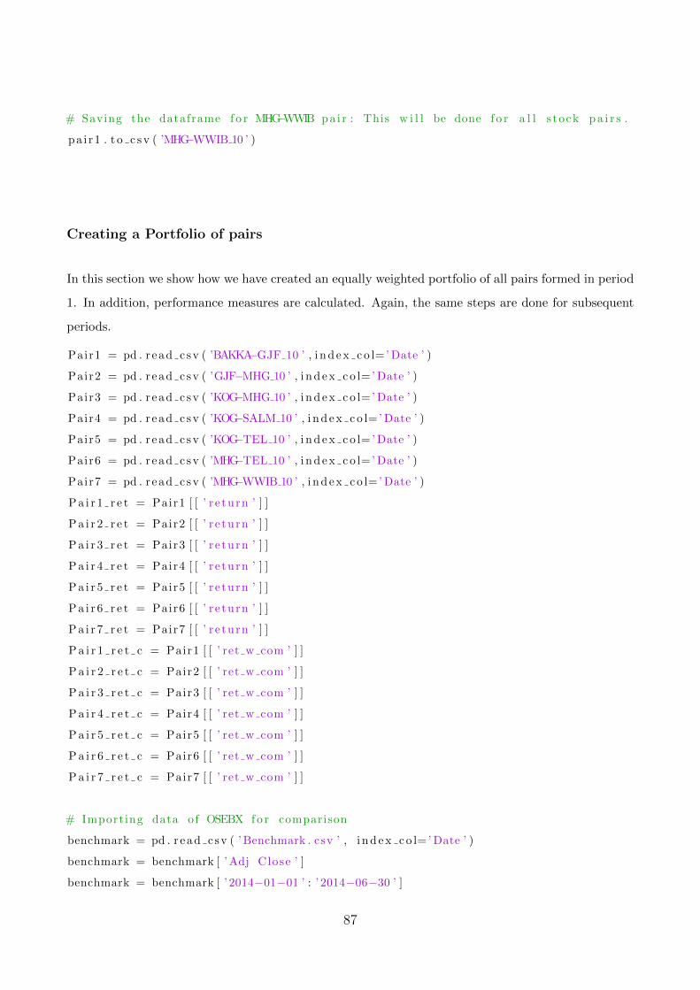
# Saving the dataframe f o r MHG−WWIB pa i r : This w i l l be done f o r a l l s tock p a i r s .
pa i r1 . t o c s v ( ’MHG−WWIB 10 ’ )
Creating a Portfolio of pairs
In this section we show how we have created an equally weighted portfolio of all pairs formed in period
1. In addition, performance measures are calculated. Again, the same steps are done for subsequent
periods.
Pair1 = pd . r ead c sv ( ’BAKKA−GJF 10 ’ , i n d e x c o l=’ Date ’ )
Pair2 = pd . r ead c sv ( ’GJF−MHG 10 ’ , i n d e x c o l=’ Date ’ )
Pair3 = pd . r ead c sv ( ’KOG−MHG 10 ’ , i n d e x c o l=’ Date ’ )
Pair4 = pd . r ead c sv ( ’KOG−SALM 10 ’ , i n d e x c o l=’ Date ’ )
Pair5 = pd . r ead c sv ( ’KOG−TEL 10 ’ , i n d e x c o l=’ Date ’ )
Pair6 = pd . r ead c sv ( ’MHG−TEL 10 ’ , i n d e x c o l=’ Date ’ )
Pair7 = pd . r ead c sv ( ’MHG−WWIB 10 ’ , i n d e x c o l=’ Date ’ )
P a i r 1 r e t = Pair1 [ [ ’ r e turn ’ ] ]
P a i r 2 r e t = Pair2 [ [ ’ r e turn ’ ] ]
P a i r 3 r e t = Pair3 [ [ ’ r e turn ’ ] ]
P a i r 4 r e t = Pair4 [ [ ’ r e turn ’ ] ]
P a i r 5 r e t = Pair5 [ [ ’ r e turn ’ ] ]
P a i r 6 r e t = Pair6 [ [ ’ r e turn ’ ] ]
P a i r 7 r e t = Pair7 [ [ ’ r e turn ’ ] ]
P a i r 1 r e t c = Pair1 [ [ ’ ret w com ’ ] ]
P a i r 2 r e t c = Pair2 [ [ ’ ret w com ’ ] ]
P a i r 3 r e t c = Pair3 [ [ ’ ret w com ’ ] ]
P a i r 4 r e t c = Pair4 [ [ ’ ret w com ’ ] ]
P a i r 5 r e t c = Pair5 [ [ ’ ret w com ’ ] ]
P a i r 6 r e t c = Pair6 [ [ ’ ret w com ’ ] ]
P a i r 7 r e t c = Pair7 [ [ ’ ret w com ’ ] ]
# Importing data o f OSEBX f o r comparison
benchmark = pd . r ead c sv ( ’ Benchmark . csv ’ , i n d e x c o l=’ Date ’ )
benchmark = benchmark [ ’ Adj Close ’ ]
benchmark = benchmark [ ’ 2014−01−01 ’ : ’ 2014−06−30 ’ ]
87
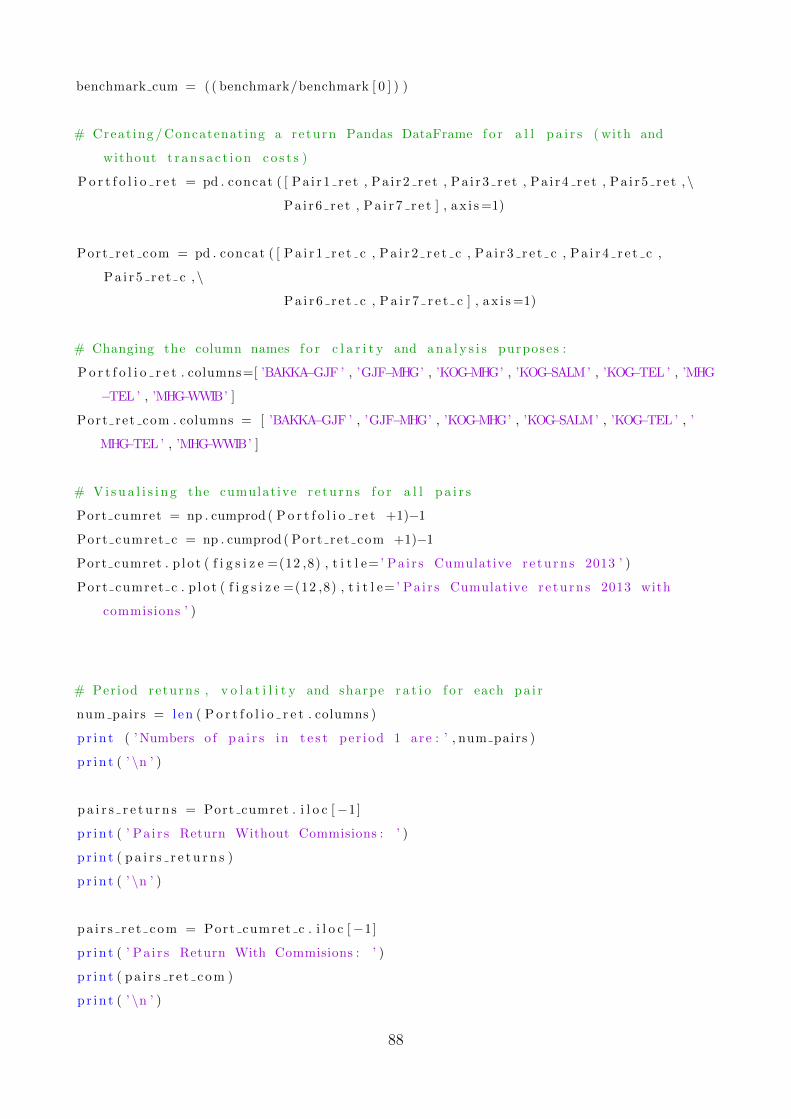
benchmark cum = ( ( benchmark/benchmark [ 0 ] ) )
# Creat ing / Concatenating a return Pandas DataFrame f o r a l l p a i r s ( with and
without t r a n s a c t i o n c o s t s )
P o r t f o l i o r e t = pd . concat ( [ Pa i r1 r e t , Pa i r2 r e t , Pa i r3 r e t , Pa i r4 r e t , Pa i r5 r e t ,\
Pa i r6 r e t , P a i r 7 r e t ] , a x i s =1)
Port ret com = pd . concat ( [ P a i r 1 r e t c , P a i r 2 r e t c , P a i r 3 r e t c , P a i r 4 r e t c ,
P a i r 5 r e t c ,\
P a i r 6 r e t c , P a i r 7 r e t c ] , a x i s =1)
# Changing the column names f o r c l a r i t y and a n a l y s i s purposes :
P o r t f o l i o r e t . columns=[ ’BAKKA−GJF ’ , ’GJF−MHG’ , ’KOG−MHG’ , ’KOG−SALM’ , ’KOG−TEL ’ , ’MHG
−TEL ’ , ’MHG−WWIB’ ]
Port ret com . columns = [ ’BAKKA−GJF ’ , ’GJF−MHG’ , ’KOG−MHG’ , ’KOG−SALM’ , ’KOG−TEL ’ , ’
MHG−TEL ’ , ’MHG−WWIB’ ]
# V i s u a l i s i n g the cumulat ive r e tu rn s f o r a l l p a i r s
Port cumret = np . cumprod ( P o r t f o l i o r e t +1)−1
Port cumret c = np . cumprod ( Port ret com +1)−1
Port cumret . p l o t ( f i g s i z e =(12 ,8) , t i t l e=’ Pa i r s Cumulative r e tu rn s 2013 ’ )
Port cumret c . p l o t ( f i g s i z e =(12 ,8) , t i t l e=’ Pa i r s Cumulative r e tu rn s 2013 with
commisions ’ )
# Period returns , v o l a t i l i t y and sharpe r a t i o f o r each pa i r
num pairs = len ( P o r t f o l i o r e t . columns )
p r i n t ( ’ Numbers o f p a i r s in t e s t per iod 1 are : ’ , num pairs )
p r i n t ( ’ \n ’ )
p a i r s r e t u r n s = Port cumret . i l o c [−1]
p r i n t ( ’ Pa i r s Return Without Commisions : ’ )
p r i n t ( p a i r s r e t u r n s )
p r i n t ( ’ \n ’ )
p a i r s r e t c o m = Port cumret c . i l o c [−1]
p r i n t ( ’ Pa i r s Return With Commisions : ’ )
p r i n t ( p a i r s r e t c o m )
pr in t ( ’ \n ’ )
88
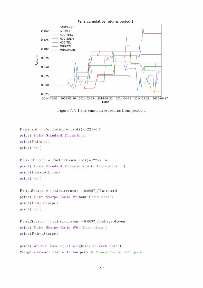
Figure 7.7: Pairs cumulative returns from period 1
P a i r s s t d = P o r t f o l i o r e t . s td ( ) ∗122∗∗0.5
p r i n t ( ’ Pa i r s Standard Dev iat ions : ’ )
p r i n t ( P a i r s s t d )
p r i n t ( ’ \n ’ )
Pa i r s s td com = Port ret com . std ( ) ∗122∗∗0.5
p r i n t ( ’ Pa i r s Standard Dev iat ions with Commisions : ’ )
p r i n t ( Pa i r s s td com )
pr in t ( ’ \n ’ )
Pa i r s Sharpe = ( p a i r s r e t u r n s −0.0097)/ P a i r s s t d
p r in t ( ’ Pa i r s Sharpe−Ratio Without Commisions ’ )
p r i n t ( Pa i r s Sharpe )
p r i n t ( ’ \n ’ )
Pa i r s Sharpe = ( p a i r s r e t c o m −0.0097)/ Pa i r s s td com
pr in t ( ’ Pa i r s Sharpe−Ratio With Commisions ’ )
p r i n t ( Pa i r s Sharpe )
p r i n t ( ’We w i l l have equal we ight ing in each pa i r ’ )
We ight s in each pa i r = 1/ num pairs # A l l o c a t i o n to each pa i r :
89
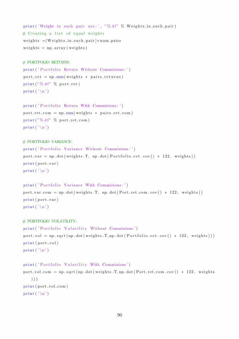
pr in t ( ’ Weight in each pa i r are : ’ , ”%.4 f ” % Weight s in each pa i r )
# Creat ing a l i s t o f equal weights
weights =[ We ight s in each pa i r ]∗ num pairs
weights = np . array ( weights )
# PORTFOLIO RETURNS:
p r i n t ( ’ P o r t f o l i o Return Without Commisions : ’ )
p o r t r e t = np . sum( weights ∗ p a i r s r e t u r n s )
p r i n t ( ”%.4 f ” % p o r t r e t )
p r i n t ( ’ \n ’ )
p r i n t ( ’ P o r t f o l i o Return With Commisions : ’ )
por t re t com = np . sum( weights ∗ p a i r s r e t c o m )
pr in t ( ”%.4 f ” % port re t com )
pr in t ( ’ \n ’ )
# PORTFOLIO VARIANCE:
p r in t ( ’ P o r t f o l i o Variance Without Commisions : ’ )
po r t var = np . dot ( weights .T, np . dot ( P o r t f o l i o r e t . cov ( ) ∗ 122 , weights ) )
p r i n t ( por t var )
p r i n t ( ’ \n ’ )
p r i n t ( ’ P o r t f o l i o Variance With Commisions : ’ )
port var com = np . dot ( weights .T, np . dot ( Port ret com . cov ( ) ∗ 122 , weights ) )
p r i n t ( por t var )
p r i n t ( ’ \n ’ )
# PORTFOLIO VOLATILITY:
p r in t ( ’ P o r t f o l i o V o l a t i l i t y Without Commisions ’ )
p o r t v o l = np . s q r t (np . dot ( weights .T, np . dot ( P o r t f o l i o r e t . cov ( ) ∗ 122 , weights ) ) )
p r i n t ( p o r t v o l )
p r i n t ( ’ \n ’ )
p r i n t ( ’ P o r t f o l i o V o l a t i l i t y With Commisions ’ )
port vo l com = np . s q r t (np . dot ( weights .T, np . dot ( Port ret com . cov ( ) ∗ 122 , weights
) ) )
p r i n t ( port vo l com )
pr in t ( ’ \n ’ )
90

# SHARPE RATIO:
p r in t ( ’ Sharpe−Ratio Without Commisions : ’ )
SR = ( po r t r e t −0.0097) / p o r t v o l
p r i n t (SR)
p r in t ( ’ \n ’ )
p r i n t ( ’ Sharpe Ratio With Commisions : ’ )
SR = ( port ret com −0.0097) / port vo l com
pr in t (SR)
# For−loop f o r p o r t f o l i o without commisions :
f o r p a i r s d f in ( Pa i r1 r e t , Pa i r2 r e t , Pa i r3 r e t , Pa i r4 r e t , Pa i r5 r e t , Pa i r6 r e t ,
P a i r 7 r e t ) :
p a i r s d f [ ’Normed Return ’ ] = np . cumprod ( p a i r s d f [ ’ r e turn ’ ]+1)
# For−loop f o r p o r t f o l i o with commisions :
f o r p a i r s d f 2 in ( P a i r 1 r e t c , P a i r 2 r e t c , P a i r 3 r e t c , P a i r 4 r e t c , P a i r 5 r e t c ,
P a i r 6 r e t c , P a i r 7 r e t c ) :
p a i r s d f 2 [ ’Normed Return ’ ] = np . cumprod ( p a i r s d f 2 [ ’ ret w com ’ ]+1)
# For−loop f o r p o r t f o l i o without commisions :
f o r p a i r s d f , a l l o in z ip ( ( Pa i r1 r e t , Pa i r2 r e t , Pa i r3 r e t , Pa i r4 r e t , Pa i r5 r e t ,
Pa i r6 r e t , P a i r 7 r e t ) , we ights ) :
p a i r s d f [ ’ A l l o c a t i o n ’ ] = p a i r s d f [ ’Normed Return ’ ]∗ a l l o
# For−loop f o r p o r t f o l i o with commisions :
f o r p a i r s d f 2 , a l l o 2 in z ip ( ( P a i r 1 r e t c , P a i r 2 r e t c , P a i r 3 r e t c , P a i r 4 r e t c ,
P a i r 5 r e t c , P a i r 6 r e t c , P a i r 7 r e t c ) , weights ) :
p a i r s d f 2 [ ’ A l l o c a t i o n ’ ] = p a i r s d f 2 [ ’Normed Return ’ ]∗ a l l o 2
a l l p a i r s i n p o r t = [ P a i r 1 r e t [ ’ A l l o c a t i o n ’ ] , P a i r 2 r e t [ ’ A l l o c a t i o n ’ ] , P a i r 3 r e t [ ’
A l l o ca t i o n ’ ] , P a i r 4 r e t [ ’ A l l o c a t i o n ’ ] ,\
P a i r 5 r e t [ ’ A l l o c a t i o n ’ ] , P a i r 6 r e t [ ’ A l l o c a t i o n ’ ] , P a i r 7 r e t [ ’
A l l o ca t i o n ’ ] ]
po r t f o l i o cum = pd . concat ( a l l p a i r s i n p o r t , a x i s =1)
a l l p a i r s i n p o r t 2 = [ P a i r 1 r e t c [ ’ A l l o c a t i on ’ ] , P a i r 2 r e t c [ ’ A l l o c a t i on ’ ] ,
P a i r 3 r e t c [ ’ A l l o c a t i on ’ ] , P a i r 4 r e t c [ ’ A l l o c a t i on ’ ] ,\
P a i r 5 r e t c [ ’ A l l o c a t i on ’ ] , P a i r 6 r e t c [ ’ A l l o c a t i on ’ ] ,
P a i r 7 r e t c [ ’ A l l o c a t i on ’ ] ]
91
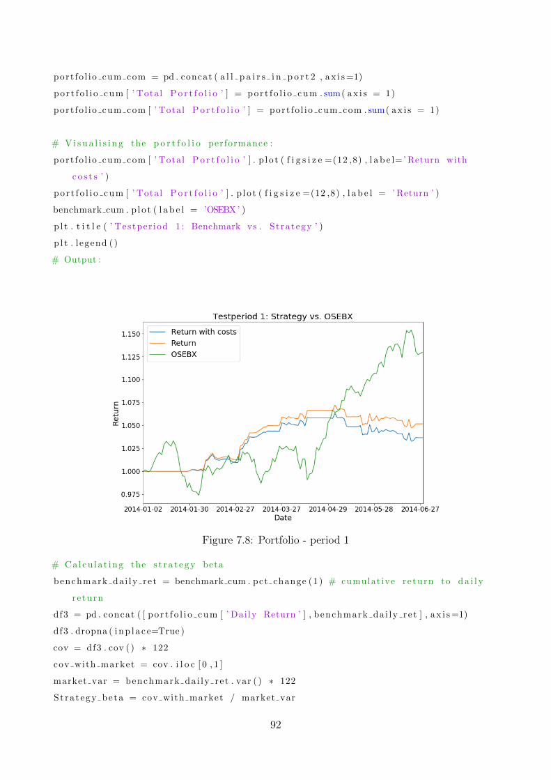
port fo l io cum com = pd . concat ( a l l p a i r s i n p o r t 2 , a x i s =1)
po r t f o l i o cum [ ’ Total P o r t f o l i o ’ ] = por t f o l i o cum . sum( a x i s = 1)
port fo l io cum com [ ’ Total P o r t f o l i o ’ ] = port fo l io cum com . sum( a x i s = 1)
# V i s u a l i s i n g the p o r t f o l i o performance :
port fo l io cum com [ ’ Total P o r t f o l i o ’ ] . p l o t ( f i g s i z e =(12 ,8) , l a b e l=’ Return with
c o s t s ’ )
po r t f o l i o cum [ ’ Total P o r t f o l i o ’ ] . p l o t ( f i g s i z e =(12 ,8) , l a b e l = ’ Return ’ )
benchmark cum . p l o t ( l a b e l = ’OSEBX’ )
p l t . t i t l e ( ’ Testper iod 1 : Benchmark vs . St rategy ’ )
p l t . l egend ( )
# Output :
Figure 7.8: Portfolio - period 1
# Calcu l a t ing the s t r a t e g y beta
benchmark da i ly re t = benchmark cum . pct change (1 ) # cumulat ive re turn to d a i l y
re turn
df3 = pd . concat ( [ po r t f o l i o cum [ ’ Dai ly Return ’ ] , benchmark da i ly re t ] , a x i s =1)
df3 . dropna ( i n p l a c e=True )
cov = df3 . cov ( ) ∗ 122
cov with market = cov . i l o c [ 0 , 1 ]
market var = benchmark da i ly re t . var ( ) ∗ 122
St ra t egy be ta = cov with market / market var
92
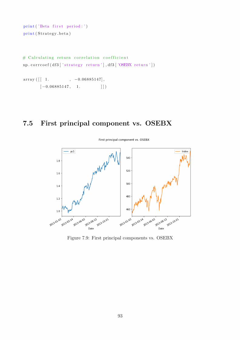
pr in t ( ’ Beta f i r s t per iod : ’ )
p r i n t ( S t ra t egy be ta )
# Ca l cu l a t ing return c o r r e l a t i o n c o e f f i c i e n t
np . c o r r c o e f ( df3 [ ’ s t r a t e g y return ’ ] , df3 [ ’OSEBX return ’ ] )
array ( [ [ 1 . , −0.06885147] ,
[−0.06885147 , 1 . ] ] )
7.5 First principal component vs. OSEBX
Figure 7.9: First principal components vs. OSEBX
93


