Embed Size (px)
Citation preview

“EnerMarket: jem080307nm” — 2008/6/18 — 21:17 — page 3 — #1
The Journal of Energy Markets (3–33) Volume 1/Number 2, Summer 2008
Performance of statistical arbitragein petroleum futures markets
Amir H. AlizadehFaculty of Finance, Cass Business School, 106 Bunhill Row, London EC1Y 8TZ, UK;email: [email protected]
Nikos K. NomikosFaculty of Finance, Cass Business School, 106 Bunhill Row, London EC1Y 8TZ, UK;email: [email protected]
This paper investigates the intermarket and intercommodity linkages ofpetroleum and petroleum product futures markets and proposes tradingstrategies based on the combination of fundamental and technical analy-ses. These trading strategies use the cointegration between futures prices asfundamental relationships and implement technical trading rules to deter-mine timing of long-short positions. The robustness of the trading strategiesis also tested using the stationary bootstrap approach. Our results indi-cate that expected market prices in the relative form (spreads) incorporateinefficiencies, which can be translated to abnormal profits through appro-priate trading strategies even when high levels of transaction costs (bid-askspreads) are considered.
1 INTRODUCTION
Energy markets function with a unique structure of supply and demand mecha-nisms, which introduce a degree of complexity along with significant levels ofuncertainty. After the two oil price crises in the 1970s, individual investors andenergy market participants have always been faced with high levels of volatility,which in turn create the opportunity for large profits from speculation on oil prices.However, at the same time, this volatility can also lead to large losses if investmentstrategies are implemented at the wrong phase of the cycle. Within this setting, theformulation of sound trading strategies in the petroleum futures market is essentialand can make the difference between success and failure of investment decisions.
The main body of literature on physical and derivatives oil markets concentrateson issues such as price discovery, market interrelationships and hedging effective-ness. For example, the issue of price discovery and efficiency has been investigatedby Crowder and Hamed (1993), who find that West Texas Intermediate (WTI)
The author would like to thank Mr Panos Pouliasis for meticulous research assistance. Thehelpful comments of participants at the 2006 Energy Risk Europe Conference in London arealso appreciated. The usual disclaimer applies.
1234567891011121314151617181920212223242526272829303132333435363738394041424344N
3

“EnerMarket: jem080307nm” — 2008/6/18 — 21:17 — page 4 — #2
4 A. H. Alizadeh and N. K. Nomikos
futures are unbiased forecasts of the realized spot prices. Other studies investigatethe causal relationship between oil spot and futures prices. For example, Silvapulleand Moosa (1999) report that oil spot and futures prices react simultaneously tothe arrival of new information to the market. Haigh and Holt (2002) account forvolatility spillovers between the crude, unleaded gasoline and heating oil markets,by using a multivariate error correction GARCH model to simultaneously link allthree futures and spot markets and further estimate the minimum variance hedgeratio for the crack spread.1 Making an allowance for transaction costs and carryingout in- and out-of-sample tests, they report substantial risk reduction comparedwith alternative hedging strategies.
A number of studies also investigate linkages between physical and futurescrude oil markets in different geographical locations. For instance, Ewing andHarter (2000) provide evidence that Brent blend and Alaska North Slope crudeoil prices move together over time and react similarly to shocks in the world oilmarket. Milonas and Henker (2001) investigate the relationship between Brentand WTI, modeling the two futures spread as a function of the convenience yieldsof the two contracts. They use convenience yields as surrogates for supply anddemand conditions in the two markets and find that they can explain the variationin the intercrude spread. Alizadeh and Nomikos (2004) find that WTI futures andfreight rates are cointegrated, whereas physical Brent and Nigerian Bonny, as wellas the spread between futures and physical prices, are not related to freight rates.This is violating the cost of carry relationship, which in turn indicates the existenceof arbitrage opportunities. The findings of these studies indicate that oil marketsaround the world are linked and prices move together over time.
A common feature of all those studies is that they either concentrate on the rela-tionship between spot and futures prices in one market or investigate the linkagesbetween spot and futures prices in different markets. Given the exacerbated volatil-ity of oil prices, the global nature of energy commodities and the frequent supplychain disruptions and demand shocks, the oil market attracts a lot of interest fromspeculators. Consequently, the issue of whether profitable trading opportunitiesexist has been investigated extensively in the market.
Girma and Paulson (1999) investigate the profitability of trading opportuni-ties for petroleum futures spreads traded on the New York Mercantile Exchange(NYMEX). They find that crack spread series are stationary and can be used to setup profitable moving average (MA) trading rules. They argue that the existence ofstrong long-term relationship among the spreads can justify the use of MA rules toidentify departures from equilibrium; otherwise, if the spread is non-stationary, itwill deviate without boundaries, and its use for either risk management or specula-tion will involve a high degree of uncertainty. However, although they report profits
1 A crack spread is the simultaneous purchase (sale) of crude oil futures and sale (purchase) ofpetroleum product futures. The crack spreads are 3:2:1 crack (ie, three barrels of crude oil againsttwo barrels of gasoline and one barrel of heating oil), 1:1:0 gasoline crack and 1:0:1 heating oilcrack, and their magnitude reflects the cost of refining crude oil into petroleum products plusany profit/loss to refineries.
1234567891011121314151617181920212223242526272829303132333435363738394041424344N
The Journal of Energy Markets Volume 1/Number 2, Summer 2008

“EnerMarket: jem080307nm” — 2008/6/18 — 21:17 — page 5 — #3
Performance of statistical arbitrage in petroleum futures markets 5
significantly different from zero, overall, the employed trading rules might not beas good as they promise and, as they state, “one cannot be certain that these oppor-tunities still exist” if a different sample is used. Consequently, their analysis ismerely a historical evaluation of risk arbitrage opportunities in petroleum futuresspreads, because results from technical trading rules are prone to data snoop-ing. The same drawbacks are also evident in another study of the crack spreadrelationship by Poitras and Teoh (2003). They explore day trading opportunitiesin the NYMEX market, using opening and closing (settlement) prices. Overall,they report net transaction fees profits, subject to some filter size that regulatesthe sensitivity of the trade signals to the actual decision of initiating a position.Other empirical studies that concentrate on commodities spread trading includeWahab et al (1994) for the gold-silver spread, Johnson et al (1991) for the crushspread in the soybean complex, Emery and Liu (2002) for spark spreads con-structed from NYMEX contracts and Liu (2005) for spreads among hog, corn andsoybean meal futures.
The study by Dunis et al (2006a) employs an alternative procedure by modelingand forecasting the spread. The data set used was comprised of daily closing pricesof NYMEX WTI and Intercontinental Exchange (ICE) Brent. They use five tradingmodels: fair value cointegration, MA, autoregressive moving average (ARMA),genaralized autoregressive conditional heteroskedasticity (GARCH) and the neuralnetwork regression.2 The sample (1995–2004) is split into two periods, one forin-sample and one for out-sample testing. The best models proved to be theARMAand the MA. However, the question whether the results would be qualitatively thesame, using a different data set is not answered (data snooping).
This paper’s objective is to investigate the relationship between the differentpairs of petroleum and petroleum products futures spreads and utilize these link-ages to establish trading strategies that make use of statistical arbitrage tradingopportunities. Till now, literature has been focused on investigating linkages inthe WTI – Brent futures or the NYMEX 3:2:1 crack spread, the unleaded gasolineand/or the heating oil crack spread. However, such strategies have been evalu-ated on the basis of their historical performance. Since technical trading strategiesare prone to data snooping, one should confirm the robustness of such strategies,using also out-of-sample tests, before making inferences. In this study, in orderto discount the possibility of data snooping bias, we use bootstrap simulations.In addition, another important question that has not been investigated in the oilspreads market literature is whether the profits produced by different strategies aresignificantly greater than other benchmark strategies. The profitability and risk-return characteristics of the employed trading strategies are compared with a simple
2 The study by Dunis et al (2006b) focuses on artificial neural networks. In this study, threeneural network models are used, namely multi-layer perceptron, recurrent and higher orderneural network. They examine trading strategies for an equally weighted portfolio of six spreads,containing WTI, Brent, Unleaded Gasoline and Heating oil futures contracts. The best out-of-sample model is the recurrent neural network with a transitive filter.
1234567891011121314151617181920212223242526272829303132333435363738394041424344N
Research Paper www.thejournalofenergymarkets.com
“EnerMarket: jem080307nm” — 2008/6/18 — 21:17 — page 6 — #4
6 A. H. Alizadeh and N. K. Nomikos
benchmark strategy, where one has a long position in the petroleum futures market,all the time. This comparison enables us to assess whether the dynamic strategy offrequent rebalancing according to signals specified by the behavior of price differ-entials among petroleum futures is superior to static trading strategies. In doing so,we also consider the direction of causality and lead or lag relationships betweenthese two markets. Furthermore, we also provide a framework for identifying devi-ations from long-run relationships among different petroleum futures markets thatmay lead to profitable trading positions. Hence, the intention of this paper is fillingthe gap in the oil market literature by providing evidence for trading opportunities.The study is concentrated on the intermarket and intercommodity linkages betweenthe possible combinations of two NYMEX and two ICE futures contracts, namelyWTI crude oil and NYMEX heating oil and ICE Brent crude oil and ICE gas oil,respectively. In- and out-of-sample tests of the suggested strategies versus alter-native benchmarks validate inferences about the performance of such strategies.
The structure of this paper is as follows: Sections 2 and 3 present the statisticalmethodology and the empirical model of this study, respectively; the propertiesof the data are discussed in Section 4; Section 5 offers the empirical results; andSections 6 and 7 describe the performance of the employed strategies and theconclusions, respectively.
2 STATISTICAL METHODOLOGY
To investigate the relationship between the cross combinations of the petroleumfutures contracts, causality and error correction is of paramount importance. Thepairs’ causal relationship can be examined by using the following vector errorcorrection model (VECM) (Johansen (1988)):
�Xt =p−1∑
i=1
�i�Xt−1 + �Xt−1 + εt, εt ∼ N(0, �) (1)
where Xt is a 2 × 1 vector of futures prices, each being I(1) such that the firstdifferenced series are I(0); � denotes the first difference operator; �i and � are2 × 2 coefficient matrices measuring the short- and long-run adjustment of thesystem to changes in Xt, respectively; and εt is a 2 × 1 vector of the vector ofGaussian stationary white noise processes with constant covariance matrix �.
The following steps are involved in our analysis. First, the existence of a sta-tionary relationship between different pairs of futures prices is investigated in theVECM of Equation (1) through the λmax and λtrace statistics (Johansen (1988)),which test for the rank (�). The rank (�) in turn determines the number of cointe-grating relationships. If � has a full rank, that is 2, then all the variables in Xt areI(0) and the appropriate modeling strategy is to estimate a vector autoregressive(VAR) model in levels. If rank (�) = 0, � is a 2 × 2 null matrix and the VECMof Equation (1) is reduced to a VAR model in first differences. On the other hand,if � has a reduced rank, that is, then there exists one cointegrating vector and the
1234567891011121314151617181920212223242526272829303132333435363738394041424344N
The Journal of Energy Markets Volume 1/Number 2, Summer 2008

“EnerMarket: jem080307nm” — 2008/6/18 — 21:17 — page 7 — #5
Performance of statistical arbitrage in petroleum futures markets 7
coefficient matrix � can be decomposed as � = αβ′, where α and β′ are 2 × 1vectors. Using this factorization, β′ represents the vector of cointegrating param-eters and α is the vector of error correction coefficients measuring the speed ofconvergence to the long-run steady state.
Second, if the pairs of futures prices are cointegrated, then causality mustexist in at least one direction (Granger (1986)). A time series, say WTIt , is said toGranger cause another time series, say Brentt , if the present values of Brentt can bepredicted more accurately by using past values of WTIt than by not doing so, con-sidering also other relevant information including past values of Brentt (Granger(1969)). If both WTIt and Brentt Granger cause each other, then there is a two-wayfeedback relationship between the two markets. The VECM of Equation (1) pro-vides a framework for valid inference in the presence of I(1) variables. Moreover,modeling the series using the Johansen (1988) procedure results in more efficientestimates of the cointegrating relationship than the Engle and Granger (1987)estimator (see Gonzalo (1994)). In addition, Johansen (1988) tests are shown tobe fairly robust to the presence of non-normality (Cheung and Lai (1993)) andheteroskedastic disturbances (Lee and Tse (1996)).
If F1,t and F2,t are the logprices of the two legs of the constructed spread at time t,the comovement and linkage between petroleum futures contracts can be examinedusing the VECM of Equation (1). The short-run price dynamics are expressed bythe lagged cross-market terms, whereas the long-run price processes are reflectedin the cointegration vector. The important element of the established cointegratingrelationship is the error correction term (ECT), which can be regarded as the spreadbetween logfutures prices (β1F1,t − β2F2,t − β0). In particular, the intercept termin the ECT, β0, represents the long-run equilibrium relationship or the averagespread.3
3 TRADING STRATEGIES
The aim of the cointegration analysis is to investigate the relationship betweenthe different pairs of petroleum futures and then to develop a trading strategy thatutilizes this relationship to identify investment timing opportunities. Therefore, wemake use of the historical correlation and cointegration of the prices as indicators ofmarketmovementsand, consequently, assignals forbuyingand/orsellingdecisions.
In practice, one can devise limitless trading rules and strategies, as there aremultiple combinations of relationships between variables that can produce a tradingsignal and multiple parameterizations for a given family of rules. For instance,there are different combinations of MA rules reflecting different time spans in theestimation of MA prices; similarly, there are numerous parameterizations of filterrules, depending on how many standard deviations one allows before reversinga position. As it is beyond scope of this study to evaluate an exhaustive set of
3 If rank (�) = 0, spreading is not justified because zero rank means that the two-leggedpositions will tend to drift apart over time.
1234567891011121314151617181920212223242526272829303132333435363738394041424344N
Research Paper www.thejournalofenergymarkets.com

“EnerMarket: jem080307nm” — 2008/6/18 — 21:17 — page 8 — #6
8 A. H. Alizadeh and N. K. Nomikos
trading rules, we focus our efforts on three simple cases of MA rules, based ondifferent petroleum futures spreads, to identify departures of the differential fromthe long-run equilibrium relationship.
MA trading strategies are based on the comparison of one fast (short) and oneslow (long) MA of the spread of futures prices. For example, one such strategyis to compare a three-month MA of the spread with a one-week MA of the sameseries. In this setting, in any given month, a positive difference between the three-month MA and the one-week MA of the spread indicates a buy decision. This isbecause when the three-month MA is greater than the one-week MA, this can beinterpreted as the series being below the long-run average (which is representedby the three-month MA). Consequently, this implies that the spread is lower thanits long-run average or, alternatively, that the futures prices of the one commodityare undervalued relative to the other.
4 DESCRIPTION OF THE DATA AND PRELIMINARY ANALYSIS
Thedataset for this studycomprisesweekly futuresprices for fourenergycommodi-ties: NYMEX WTI crude oil, NYMEX heating oil, ICE Brent crude oil and ICEgas oil, covering the period August 9, 1989, to September 20, 2006, resulting 894weekly observations. Futures prices are Wednesday prices; when a holiday occurson Wednesday, Tuesday’s observation is used. Data is collected from Datastream.
Nowadays, there are two major exchanges providing oil-derivative contracts:NYMEX and ICE in London. Other exchanges that trade oil-related contractsare the Tokyo Commodity Exchange (TOCOM) since 1999 (crude oil, gas oil,gasoline and kerosene futures) and the Dubai Mercantile Exchange (DME) since2006, which constitutes the first energy futures exchange in the Middle East. Thisstudy concentrates on NYMEX and ICE futures, where the data set is sufficientfor a weekly based analysis. NYMEX WTI contracts are traded for all deliverieswithin the next 30 consecutive months as well as for specific long-dated deliveriessuch as 36, 48, 72 and 84 months from delivery. Each contract is traded until theclose of business on the third business day prior to the 25th calendar day of themonth preceding the delivery month. NYMEX heating oil contracts are traded forall deliveries within the next 18 months and each contract of NYMEX heating oil isterminated on the last business day of the month preceding the delivery month. ICEBrent crude oil contracts are traded for all deliveries within the next 30 consecutivemonths and then half-yearly out to a maximum of seven years. Each contract istraded until the close of business on the business day immediately preceding the15th day prior to the first day of the delivery month. ICE gas oil contracts aretraded for all deliveries for 12 consecutive months forward, then quarterly out to24 months and then half-yearly out to 36 months. Contracts expire two businessdays prior to the 14th calendar day of the delivery month.
Since the contracts’ expiration dates are not matching, it is assumed that theinvestor will roll over to the front month pair of contracts, the first day of the lasttrading month. For instance, the February 2001 ICE Brent crude oil contract (for
1234567891011121314151617181920212223242526272829303132333435363738394041424344N
The Journal of Energy Markets Volume 1/Number 2, Summer 2008

“EnerMarket: jem080307nm” — 2008/6/18 — 21:17 — page 9 — #7
Performance of statistical arbitrage in petroleum futures markets 9
delivery in March 2001) expired on Tuesday, January 16, and the February 2001NYMEX heating oil contract (for delivery in March 2001) expired on Wednesday,January 30. Consequently, the spread is constructed as February 2001 ICE crudeoil – NYMEX heating oil. Switching to the front month pair of contracts occurssimultaneously on the first day of the expiration month for those contracts; thatis on Wednesday, January 3, 2001, when the spread becomes March 2001 ICEcrude oil – NYMEX heating oil, we call this spread the one-month spread. Thisway we ensure that the spreads are measured at the same point in time and wealso avoid problems associated with thin trading and expiration effects, as thesespreads are always liquid. In the same way, for the two-month spread, rollingover occurs on the first day of the month preceding the expiration month and soon. Having constructed the four continuous time series for the futures contracts,futures prices are then converted to the same unit of measure; that is US dollarsper barrel (US$/bbl). Prices are then transformed to natural logarithms, and thenthe spreads are constructed, as discussed above.
Descriptive statistics of the one-, two-, three- and four-month spreads indicatethat the spread series are serially correlated, heteroskedastic and non-normal. Inaddition, unit root tests reveal that all crude and petroleum futures prices aredifference stationary. The spread series, on the other hand, are stationary, indicatingthat the VECM specification is the appropriate tool to uncover the relationshipsand mean-reverting properties of the spread series.4
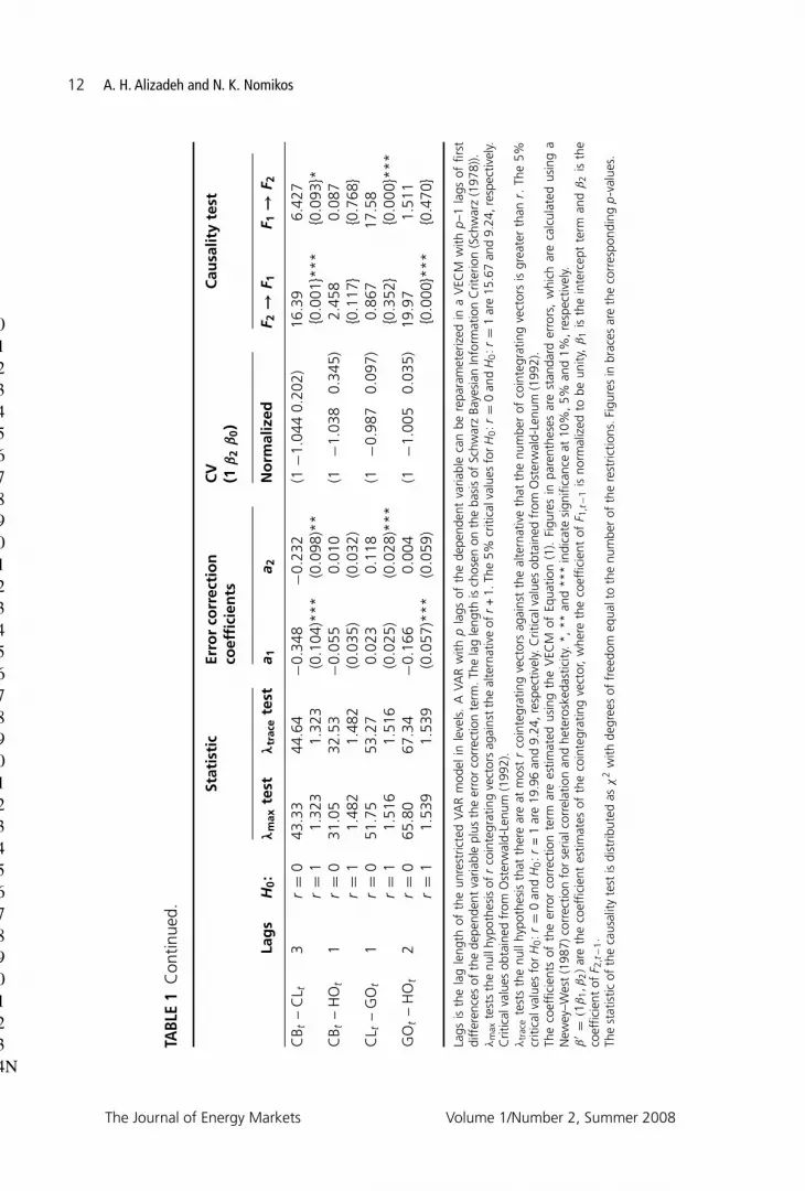
5 EMPIRICAL RESULTS
Cointegration techniques are employed next to investigate the existence of along-run relationship between the time series. The lag length of the VECM ofEquation (1) is chosen on the basis of the Schwarz Bayesian Information Crite-rion (SBIC) (Schwarz (1978)). Johansen (1988) cointegration tests, presented inTable 1, indicate that all oil futures prices stand in a long-run relationship with eachother. Since this condition is met, the pairs of futures prices evolve in proximity toone another, and any deviation from this relationship signals a trading opportunity,as cointegration implies that this departure will be restored. The normalized coef-ficient estimates of the cointegrating vector β′ = (β1β2β0) represent this long-runrelationship between the series. Since the asymptotic distributions of the cointe-gration test statistics are dependent upon the presence of deterministic terms inthe VECM, it is important to validate the inclusion or not of constant and/or lineartrends in the system. Likelihood ratio tests5 indicate that an intercept term shouldbe included in the long-run relationship. The inclusion of an intercept term is alsojustified on the basis that it may capture the impact of constant parameters such
4 To save space, descriptive statistics are not presented but are available from the authors.5 These tests follow Johansen (1991). The results are not presented here and are available fromthe authors.
1234567891011121314151617181920212223242526272829303132333435363738394041424344N
Research Paper www.thejournalofenergymarkets.com

“EnerMarket: jem080307nm” — 2008/6/18 — 21:17 — page 10 — #8
10 A. H. Alizadeh and N. K. Nomikos
TABL
E1
Joha
nsen
coin
tegr
atio
nte
sts
for
petr
oleu
mfu
ture
ssp
read
s.
Stat
isti
cEr
ror
corr
ecti
on
CV
Cau
salit
yte
stco
effi
cien
ts(1
β2
β0)
Lag
sH
0:
λm
axte
stλ
trac
ete
sta 1
a 2N
orm
aliz
edF 2
→F 1
F 1→
F 2
Pane
lA:O
ne-m
onth
futu
res
CB t
–G
Ot
2r
=0
33.3
134
.76
0.01
60.
091
(1−1
.012
0.23
7)1.
510
16.8
4r
=1
1.45
81.
458
(0.0
25)
(0.0
25)*
**{0
.470
}{0
.000
}***
CL t
–H
Ot
1r
=0
40.0
841
.89
−0.0
040.
077
(1−0
.978
0.07
8)0.
024
10.1
4r
=1
1.81
01.
810
(0.0
27)
(0.0
24)*
**{0
.878
}{0
.001
}***
CB t
–C
L t3
r=
028
.99
30.6
5−0
.096
−0.0
04(1
−1.0
440.
205)
1.68
38.
537
r=
11.
653
1.65
3(0
.079
)(0
.076
){0
.641
}{0
.036
}**
CB t
–H
Ot
1r
=0
42.6
344
.24
0.00
60.
090
(1−1
.022
0.29
1)0.
058
16.0
2r
=1
1.61
01.
610
(0.0
25)
(0.0
22)*
**{0
.810
}{0
.000
}***
CL t
–G
Ot
1r
=0
55.4
857
.35
0.00
40.
106
(1−0
.971
0.03
6)0.
026
14.1
1r
=1
1.86
81.
868
(0.0
25)
(0.0
28)*
**{0
.872
}{0
.000
}***
GO
t–
HO
t2
r=
055
.33
56.8
6−0
.025
0.14
2(1
−1.0
060.
040)
14.4
810
.95
r=
11.
529
1.52
9(0
.061
)(0
.052
)***
{0.0
01}*
**{0
.004
}***
Pane
lB:T
wo-
mon
thfu
ture
sC
B t–
GO
t2
r=
025
.27
26.7
50.
013
0.07
5(1
−1.0
160.
253)
1.10
717
.44
r=
11.
485
1.48
5(0
.026
)(0
.024
)***
{0.5
75}
{0.0
00}*
**C
L t–
HO
t1
r=
032
.12
33.8
00.
021
0.08
3(1
−0.9
790.
085)
0.74
510
.79
r=
11.
679
1.67
9(0
.025
)(0
.025
)***
{0.3
88}
{0.0
01}*
**C
B t–
CL t
3r
=0
33.1
734
.74
−0.2
20−0
.127
(1−1
.045
0.20
7)10
.81
4.04
5r
=1
1.57
61.
576
(0.0
85)
(0.0
82)
{0.0
13}*
*{0
.256
}C
B t–
HO
t1
r=
033
.07
34.6
00.
005
0.07
1(1
−1.0
250.
301)
0.03
08.
122
r=
11.
532
1.53
2(0
.026
)(0
.025
)***
{0.8
63}
{0.0
04}*
**
1234567891011121314151617181920212223242526272829303132333435363738394041424344N
The Journal of Energy Markets Volume 1/Number 2, Summer 2008

“EnerMarket: jem080307nm” — 2008/6/18 — 21:17 — page 11 — #9
Performance of statistical arbitrage in petroleum futures markets 11
TABL
E1
Con
tinue
d.
Stat
isti
cEr
ror
corr
ecti
on
CV
Cau
salit
yte
stco
effi
cien
ts(1
β2
β0)
Lag
sH
0:
λm
axte
stλ
trac
ete
sta 1
a 2N
orm
aliz
edF 2
→F 1
F 1→
F 2
CL t
–G
Ot
1r
=0
50.9
752
.63
0.02
10.
113
(1−0
.977
0.05
7)0.
765
16.1
3r
=1
1.66
81.
668
(0.0
24)
(0.0
28)*
**{0
.382
}{0
.000
}***
GO
t–
HO
t2
r=
058
.46
59.9
9−0
.049
0.12
9(1
−1.0
030.
032)
13.5
57.
901
r=
11.
523
1.52
3(0
.059
)(0
.054
)**
{0.0
01}*
*{0
.019
}**
Pane
lC:T
hree
-mon
thfu
ture
sC
B t–
GO
t2
r=
022
.03
23.6
60.
005
0.06
4(1
−1.0
200.
269)
1.10
018
.58
r=
11.
633
1.63
3(0
.027
)(0
.024
)***
{0.5
78}
{0.0
00}*
**C
L t–
HO
t1
r=
026
.60
28.1
70.
017
0.07
1(1
−0.9
830.
101)
0.39
07.
263
r=
11.
570
1.57
0(0
.028
)(0
.027
)***
{0.5
33}
{0.0
07}*
**C
B t–
CL t
3r
=0
37.3
238
.71
−0.2
91−0
.189
(1−1
.044
0.20
2)14
.04
4.57
0r
=1
1.39
31.
393
(0.0
96)*
**(0
.099
)*{0
.003
}***
{0.2
06}
CB t
–H
Ot
1r
=0
29.8
831
.41
−0.0
160.
047
(1−1
.029
0.31
7)0.
295
2.73
5r
=1
1.53
01.
530
(0.0
29)
(0.0
29)*
{0.5
87}
{0.0
98}*
CL t
–G
Ot
1r
=0
50.6
152
.15
0.02
80.
120
(1−0
.983
0.07
9)1.
229
16.7
2r
=1
1.53
71.
537
(0.0
25)
(0.0
29)*
**{0
.268
}{0
.000
}***
GO
t–
HO
t2
r=
064
.31
65.8
5−0
.123
0.06
5(1
−1.0
040.
032)
15.1
03.
618
r=
11.
539
1.53
9(0
.063
)*(0
.062
){0
.001
}***
{0.1
64}
Pane
lD:F
our-
mon
thfu
ture
sC
B t–
GO
t2
r=
021
.10
22.9
6−0
.014
0.04
7(1
−1.0
260.
291)
0.37
412
.58
r=
11.
857
1.85
7(0
.028
)(0
.024
)**
{0.8
29}
{0.0
02}*
**C
L t–
HO
t1
r=
025
.28
26.8
8−0
.013
0.03
5(1
−0.9
900.
122)
0.29
41.
867
r=
11.
595
1.59
5(0
.024
)(0
.026
){0
.588
}{0
.171
}
1234567891011121314151617181920212223242526272829303132333435363738394041424344N
Research Paper www.thejournalofenergymarkets.com
“EnerMarket: jem080307nm” — 2008/6/18 — 21:17 — page 12 — #10
12 A. H. Alizadeh and N. K. Nomikos
TABL
E1
Con
tinue
d.
Stat
isti
cEr
ror
corr
ecti
on
CV
Cau
salit
yte
stco
effi
cien
ts(1
β2
β0)
Lag
sH
0:
λm
axte
stλ
trac
ete
sta 1
a 2N
orm
aliz
edF 2
→F 1
F 1→
F 2
CB t
–C
L t3
r=
043
.33
44.6
4−0
.348
−0.2
32(1
−1.0
440.
202)
16.3
96.
427
r=
11.
323
1.32
3(0
.104
)***
(0.0
98)*
*{0
.001
}***
{0.0
93}*
CB t
–H
Ot
1r
=0
31.0
532
.53
−0.0
550.
010
(1−1
.038
0.34
5)2.
458
0.08
7r
=1
1.48
21.
482
(0.0
35)
(0.0
32)
{0.1
17}
{0.7
68}
CL t
–G
Ot
1r
=0
51.7
553
.27
0.02
30.
118
(1−0
.987
0.09
7)0.
867
17.5
8r
=1
1.51
61.
516
(0.0
25)
(0.0
28)*
**{0
.352
}{0
.000
}***
GO
t–
HO
t2
r=
065
.80
67.3
4−0
.166
0.00
4(1
−1.0
050.
035)
19.9
71.
511
r=
11.
539
1.53
9(0
.057
)***
(0.0
59)
{0.0
00}*
**{0
.470
}
Lags
isth
ela
gle
ngth
ofth
eun
rest
ricte
dVA
Rm
odel
inle
vels
.A
VAR
with
pla
gsof
the
depe
nden
tva
riabl
eca
nbe
repa
ram
eter
ized
ina
VEC
Mw
ithp
–1la
gsof
first
diff
eren
ces
ofth
ede
pend
ent
varia
ble
plus
the
erro
rco
rrec
tion
term
.The
lag
leng
this
chos
enon
the
basi
sof
Schw
arz
Baye
sian
Info
rmat
ion
Crit
erio
n(S
chw
arz
(197
8)).
λm
axte
sts
the
null
hypo
thes
isof
rco
inte
grat
ing
vect
ors
agai
nst
the
alte
rnat
ive
ofr
+1.
The
5%cr
itica
lval
ues
for
H0:r
=0
and
H0:r
=1
are
15.6
7an
d9.
24,r
espe
ctiv
ely.
Crit
ical
valu
esob
tain
edfr
omO
ster
wal
d-Le
num
(199
2).
λtr
ace
test
sth
enu
llhy
poth
esis
that
ther
ear
eat
mos
tr
coin
tegr
atin
gve
ctor
sag
ains
tth
eal
tern
ativ
eth
atth
enu
mbe
rof
coin
tegr
atin
gve
ctor
sis
grea
ter
than
r.Th
e5%
criti
calv
alue
sfo
rH
0:r
=0
and
H0:r
=1
are
19.9
6an
d9.
24,r
espe
ctiv
ely.
Crit
ical
valu
esob
tain
edfr
omO
ster
wal
d-Le
num
(199
2).
The
coef
ficie
nts
ofth
eer
ror
corr
ectio
nte
rmar
ees
timat
edus
ing
the
VEC
Mof
Equa
tion
(1).
Figu
res
inpa
rent
hese
sar
est
anda
rder
rors
,w
hich
are
calc
ulat
edus
ing
aN
ewey
–Wes
t(1
987)
corr
ectio
nfo
rse
rialc
orre
latio
nan
dhe
tero
sked
astic
ity.*
,**
and
***
indi
cate
sign
ifica
nce
at10
%,5
%an
d1%
,res
pect
ivel
y.β
′ =(1
β1,β
2)
are
the
coef
ficie
ntes
timat
esof
the
coin
tegr
atin
gve
ctor
,w
here
the
coef
ficie
ntof
F 1,t
−1is
norm
aliz
edto
beun
ity,β
1is
the
inte
rcep
tte
rman
dβ
2is
the
coef
ficie
ntof
F 2,t
−1.
The
stat
istic
ofth
eca
usal
ityte
stis
dist
ribut
edas
χ2
with
degr
ees
offr
eedo
meq
ualt
oth
enu
mbe
rof
the
rest
rictio
ns.F
igur
esin
brac
esar
eth
eco
rres
pond
ing
p-v
alue
s.
1234567891011121314151617181920212223242526272829303132333435363738394041424344N
The Journal of Energy Markets Volume 1/Number 2, Summer 2008
“EnerMarket: jem080307nm” — 2008/6/18 — 21:17 — page 13 — #11
Performance of statistical arbitrage in petroleum futures markets 13
as premia and discounts, insurance charges, and quality and location differentialsfor the different types of the oil commodities.
Along with the normalized coefficients of the unrestricted cointegrating vectors,Table 1 reports the estimated error correction coefficients from the VECM. Thestandard errors are corrected for heteroskedasticity and serial correlation using theNewey–West (1987) method, for all the regressions. The speed of adjustment offutures prices to their long-run relationship, measured by the α1 and α2 estimatedcoefficients, is expected to be negative in the first equation and positive in thesecond equation. This implies that in response to a positive deviation from theirlong-run relationship at period t − 1, ie, F1,t−1 − β2F2,t−1 − β0 > 0, the futuresprice of the first (second) leg of the spread will decrease (increase) in value, inorder to restore the long-run equilibrium. As it can be seen in Table 1, all thesignificant error correction coefficients have the correct sign, with the exceptionof the three- and four-month intercrude spread.
More rigorous investigation of the interactions between the variables can beobtained by performing Granger causality tests. According to the Granger (1986)representation theorem, if two prices are cointegrated, causality must exist inat least one direction. Several observations merit attention regarding the jointdynamics of the price processes. The complex structure of the oil market impliesthat great caution should be taken when making inferences about causality, becauseits direction is not known a priori. The assumption that crude oil prices are expectedto Granger cause petroleum product prices can be based on the fact that, first,crude oil prices are determined by the worldwide supply and demand as opposedto refined products where regional supply and demand dynamics are important.6
Of course, refined products are linked to the international market through crudeoil prices, which represent a significant input production cost. Second, demandfor, say WTI crude oil, is not likely to be driven by the demand for heating oilalone, since a substantial amount of the refined crude oil is transformed to otherproducts such as gasoline, naphtha and kerosene. Test for the joint significance ofthe lagged cross-market returns and ECT confirm the above setting;7 that is theexistence of one-way relationship, with crude oil leading the information discoveryprocess – in the equations for either NYMEX or ICE crude oil futures paired withICE gas oil and NYMEX heating oil across all maturities. The exceptions arethe four-month ICE Brent (NYMEX heating oil and NYMEX WTI) heating oilpairs where there is no significant lead–lag relationship. Finally, the estimates ofthe error correction coefficients, overall, in terms of magnitude and significance,
6 Crude oil dominates the world trade because its transportation is carried in large vessels andeconomies of scale are achieved. On the other hand, transportation of higher-value refinedproducts is carried in smaller vessels, is more expensive and usually is a restricted service forshorter distance routes. In general, refineries are located next to demand sources to avoid theneed for transportation, government import–export barriers, etc.7 Nevertheless, it is not unlikely for the refined product prices to pull crude oil prices, sincedemand for crude oil is derived from petroleum products’ demand, which in turn is generatedfrom transportation, industrial and residential needs.
1234567891011121314151617181920212223242526272829303132333435363738394041424344N
Research Paper www.thejournalofenergymarkets.com

“EnerMarket: jem080307nm” — 2008/6/18 — 21:17 — page 14 — #12
14 A. H. Alizadeh and N. K. Nomikos
indicate that, basically, heating oil and gas oil prices move to adjust the long-runequilibrium, whereas crude oil prices are not responsive to departures from thelong-run mean of the differential.
In the intercrude market, the first nearby spread indicates that Brent has explana-tory power on WTI futures only in the short run, but the two are not responsive tothe differential. When the horizon increases to two-, three- and four-month futures,the picture is reversed and now NYMEX WTI Granger causes ICE Brent futures,at 5% significance level. This is expected since the United States reflects by farthe largest oil consumer and importer of crude oil, and this dependency intro-duces a high degree of sensitivity of the international market to the US oil prices,which perhaps makes the WTI market dominant in terms of information discovery(see, for instance, Lin and Tamvakis (2001)). However, this is not reflected in theone-month futures prices. This can be explained by the fact that the volatility offutures prices increase as time to maturity approaches (Samuelson (1965)), becausefutures prices tend to converge to the actual spot prices and the contracts becomemore sensitive to information flows, resulting an interruption of the core lead–lagrelationship. Error correction coefficients in the Brent futures equation have thecorrect negative sign, and they are all significant except the one-month case. Thisindicates that in response to a positive shock, the price will decrease to restore thelong-run mean (spread is constructed as log-Brent minus log-WTI). In the WTIfutures equation, error correction coefficients for the three- and four-month spreadsare also negative and at 5% significance level. However, the magnitude is lowercompared with Brent, indicating that the degree of responsiveness of WTI to thespread is inferior and, actually, adjustment to restore the long-run equilibrium ismainly due to ICE Brent crude futures price movements.
In addition, Granger causality tests in Table 1 indicate that ICE gas oil is not onlyGranger caused by NYMEX heating oil, but also Granger causes NYMEX heatingoil for the one- and two-month spreads. This two-way feedback relationship holdsat 1% and 5% significance level for the one- and two-month futures, respectively.The error correction estimates have the correct sign, negative for the ICE petroleumproduct and positive for the NYMEX petroleum product, to ensure convergence inthe long run. The long-run equilibrium relationship is restored after adjustment ofheating oil prices in the one- and two-month futures prices, whereas in the three-and four-month case heating oil prices are not responsive to the differential and anypossible adjustment originates from the ICE gas oil market. One would normallyexpect response to the differential mainly from the gas oil market because it issmaller than the US heating oil market. Another reason is that, since the demandfor crude oil is driven by the demand for refined products and since the UnitedStates is the biggest importer of crude oil, increased demand in the United States ismore likely to put pressure in oil prices. Hence, ICE gas oil market is more likelyto be driven by the US market. However, the change in pattern from the shorter-to the longer-term maturities may be due to the fact that uncertainty of futureexpectations regarding prices, demand, supply, inventories and unknown weather
1234567891011121314151617181920212223242526272829303132333435363738394041424344N
The Journal of Energy Markets Volume 1/Number 2, Summer 2008

“EnerMarket: jem080307nm” — 2008/6/18 — 21:17 — page 15 — #13
Performance of statistical arbitrage in petroleum futures markets 15
conditions is relatively higher in the longer term but the responsiveness of prices tonew information is slower, and slower is the price transmission mechanism as well.
6 PERFORMANCE OF MOVING AVERAGE TRADING RULES
The trading strategy employed in this paper, which combines the fundamental rela-tionship between variables with technical trading rules, is based on the deviationof the spread from its long-run mean. In order to determine the timing of buy orsell, we devise four MA series using the differential between log futures prices:one fast [MA(1)] and three slow [MA(4), MA(8) and MA(12)]. The differencebetween the two constructed MA series is then used as an indicator that signalswhether to buy or sell in the petroleum futures spread. The signals are based onthe sign of the difference between the slow and the fast MA in such a way that apositive difference is a buy signal, while a negative difference is a sell signal. Forinstance, regarding the ICE – NYMEX intercrude spread (constructed as log-Brentminus log-WTI), if MA(8) > MA(1), then a long position on the spread will beinitiated by purchasing one ICE Brent crude oil contract and selling one NYMEXWTI crude oil contract. The position will be held until the relationship betweenthe two MA series is inverted, ie, MA(8) < MA(1). Then, simultaneously, the longposition will be closed and a short position on the ICE – NYMEX intercrude spreadwill be initiated.8 For comparison purposes, we also consider the performance ofa benchmark buy and hold strategy. The performance of this strategy reflects theincome of an investor who maintains a long outright position on the petroleumfutures market (across the whole sample period).
One important element when evaluating dynamic trading strategies is theincurred transaction cost that these strategies involve, arising from the frequentrebalancing of the portfolio of interest. For the purposes of this study, a transactioncost of 0.2% for every round trip of initiating and reversing trade is deemed reason-able. Our assumption is comparable with other studies in the literature (Dunis et al(2006b); Poitras and Teoh (2003); and Girma and Paulson (1999)). Commissioncharges (ie, any fixed fees such as brokerage and other transaction fees), on theother hand, are very low and, usually, are negligible.9
8 The exercise was repeated for the historical and bootstrap simulations, using different filterrules. We used rolling windows for standard deviations, in order to filter the signal for entryand exit points in the market. For instance, in the ICE – NYMEX intercrude spread, a longposition on the spread will be initiated if MA(8) > MA(1) + Xσ , where X is the number ofstandard deviation units. The position will be held until the relationship between the two MAseries becomes MA(8) > MA(1) – Xσ , where a short position will be initiated simultaneously.Then, the long position will be closed and a short position on the ICE – NYMEX intercrudespread will be initiated. Application of such filters did not change the results qualitatively, but ingeneral, as the filter size increased, annualized returns decreased. The filters used were ±0.25σ ,±0.5σ , ±σ and ±1.5σ , and results are available from the authors upon request.9 For instance, in the NYMEX division, the half-turn trading fee is approximately between 0.04and 0.18 cents per barrel subject to whether the trade is undertaken by a member or non-memberof the exchange (see www.nymex.com).
1234567891011121314151617181920212223242526272829303132333435363738394041424344N
Research Paper www.thejournalofenergymarkets.com

“EnerMarket: jem080307nm” — 2008/6/18 — 21:17 — page 16 — #14
16 A. H. Alizadeh and N. K. Nomikos
TABL
E2
His
toric
alan
dbo
otst
rap
sim
ulat
ion
ofth
ree-
,tw
o-an
don
e-m
onth
MA
trad
ing
stra
tegi
es.
Thre
e-m
on
thst
rate
gy
(MA
12vs
MA
1)Tw
o-m
on
thst
rate
gy
(MA
8vs
MA
1)O
ne-
mo
nth
stra
teg
y(M
A4
vsM
A1)
Shar
pe
RSh
arp
eR
Shar
pe
RM
ean
Shar
pe
imp
rove
-M
ean
Shar
pe
imp
rove
-M
ean
Shar
pe
imp
rove
-R
etSD
rati
om
ent
Ret
SDra
tio
men
tR
etSD
rati
om
ent
Pane
lA:O
nem
onth
CB t
–G
Ot
18.1
918
.08
1.00
60.
762*
**20
.60
18.0
31.
142
0.88
2**
*25
.60
(17.
84)
1.43
51.
212
***
CL t
–H
Ot
4.57
315
.75
0.29
00.
015
5.85
915
.74
0.37
20.
094
8.79
715
.69
0.56
10.
264
CB t
–C
L t3.
659
9.46
90.
386
0.16
06.
632
9.43
10.
703
0.37
4*
11.0
29.
308
1.18
40.
856
***
CB t
–H
Ot
6.00
916
.66
0.36
10.
086
4.53
516
.68
0.27
2−0
.030
7.09
316
.64
0.42
60.
164
CL t
–G
Ot
19.9
319
.41
1.02
70.
862*
**24
.42
19.2
81.
267
1.09
3**
*30
.03
19.1
11.
571
1.34
9**
*G
Ot
–H
Ot
23.0
115
.20
1.51
31.
296*
**27
.12
15.0
31.
804
1.58
2**
*29
.17
14.9
61.
950
1.73
7**
*
Pane
lB:T
wo
mon
thC
B t–
GO
t18
.88
15.7
11.
202
0.92
0**
*20
.85
15.6
51.
332
1.09
0**
*27
.71
15.4
01.
800
1.57
7**
*C
L t–
HO
t−1
.461
12.4
6−0
.117
−0.3
800.
293
12.4
50.
024
−0.2
166.
927
12.3
70.
560
0.29
5*C
B t–
CL t
3.10
87.
840
0.39
70.
075
3.73
87.
817
0.47
80.
144
4.49
57.
851
0.57
20.
246
CB t
–H
Ot
7.22
813
.17
0.54
90.
224
8.02
513
.16
0.61
00.
299
7.20
213
.18
0.54
60.
211
CL t
–G
Ot
18.6
116
.66
1.11
70.
934
***
20.5
216
.61
1.23
51.
046
***
26.1
216
.43
1.59
01.
352
***
GO
t–
HO
t25
.35
13.4
41.
886
1.55
4**
*26
.87
13.3
62.
011
1.71
9**
*24
.82
13.4
91.
840
1.58
0**
*
Pane
lC:T
hree
mon
thC
B t–
GO
t20
.23
14.7
71.
370
1.12
6**
*24
.68
14.6
11.
689
1.42
3**
*29
.06
(14.
42)
2.01
51.
730
***
CL t
–H
Ot
−4.2
8510
.70
−0.4
00−0
.570
−3.0
2610
.70
−0.2
83−0
.497
5.55
610
.63
0.52
30.
223
CB t
–C
L t3.
468
7.45
50.
465
0.12
73.
266
7.45
60.
438
0.09
34.
380
7.43
70.
589
0.17
2C
B t–
HO
t1.
914
11.6
40.
164
−0.0
073.
695
11.6
50.
317
0.06
710
.21
11.5
40.
885
0.46
4*
CL t
–G
Ot
19.0
915
.33
1.24
61.
053
***
21.7
315
.24
1.42
61.
227
***
26.7
615
.05
1.77
91.
552
***
GO
t–
HO
t26
.83
12.7
42.
106
1.80
7**
*28
.42
12.6
82.
242
1.99
8**
*27
.50
12.7
32.
160
1.87
3***
1234567891011121314151617181920212223242526272829303132333435363738394041424344N
The Journal of Energy Markets Volume 1/Number 2, Summer 2008

“EnerMarket: jem080307nm” — 2008/6/18 — 21:17 — page 17 — #15
Performance of statistical arbitrage in petroleum futures markets 17
TABL
E2
Con
tinue
d.
Thre
e-m
on
thst
rate
gy
(MA
12vs
MA
1)Tw
o-m
on
thst
rate
gy
(MA
8vs
MA
1)O
ne-
mo
nth
stra
teg
y(M
A4
vsM
A1)
Shar
pe
RSh
arp
eR
Shar
pe
RM
ean
Shar
pe
imp
rove
-M
ean
Shar
pe
imp
rove
-M
ean
Shar
pe
imp
rove
-R
etSD
rati
om
ent
Ret
SDra
tio
men
tR
etSD
rati
om
ent
Pane
lD:F
our
mon
thC
B t–
GO
t21
.50
14.2
51.
509
1.22
2***
24.6
714
.12
1.74
71.
470*
**27
.73
13.9
81.
983
1.67
5***
CL t
–H
Ot
−6.0
5910
.04
−0.6
04−0
.782
−3.5
9410
.03
−0.3
58−0
.654
2.30
510
.03
0.23
0−0
.107
CB t
–C
L t3.
833
7.65
60.
501
0.14
14.
878
7.61
50.
641
0.27
85.
986
7.58
50.
789
0.33
8C
B t–
HO
t0.
903
11.0
50.
082
−0.1
851.
733
11.0
60.
157
−0.2
136.
791
11.0
00.
617
0.21
0C
L t–
GO
t19
.67
14.5
21.
355
1.11
4***
21.8
614
.45
1.51
31.
252*
**25
.33
14.3
11.
770
1.54
6***
GO
t–
HO
t24
.75
12.3
22.
009
1.69
6***
25.6
712
.28
2.09
01.
762*
**26
.16
12.2
92.
129
1.85
9***
Pane
lE:B
uyan
dho
ldst
rate
gies
On
em
on
thTw
om
on
thTh
ree
mo
nth
Fou
rm
on
th
Mea
nSh
arp
eM
ean
Shar
pe
Mea
nSh
arp
eM
ean
Shar
pe
Ret
SDra
tio
Ret
SDra
tio
Ret
SDra
tio
Ret
SDra
tio
CB t
6.71
931
.00
0.21
76.
907
29.1
00.
237
7.15
027
.68
0.25
87.
400
25.8
90.
286
GO
t6.
980
32.0
50.
218
7.19
829
.90
0.24
17.
352
28.1
30.
261
7.47
026
.89
0.28
1C
L t6.
276
31.5
10.
199
6.46
929
.37
0.22
06.
724
27.7
40.
242
7.07
226
.22
0.27
0H
Ot
6.66
232
.28
0.20
66.
787
29.2
70.
232
6.90
327
.08
0.25
57.
005
25.2
40.
278
Mea
nRe
tar
eth
e%
annu
aliz
edre
turn
san
dSD
are
the
%an
nual
ized
stan
dard
devi
atio
ns.
Shar
pera
tios
are
calc
ulat
edus
ing
the
form
ula
R/S
TD.
Mea
nRe
t,SD
and
Shar
pera
tios
are
thos
efr
omth
ehi
stor
ical
sim
ulat
ion
ofth
edi
ffer
ent
stra
tegi
es.
Impr
ovem
ent
inSh
arpe
ratio
isth
eex
cess
Shar
pera
tioof
the
spre
adM
A-b
ased
trad
ing
com
pare
dw
ithth
ebu
yan
dho
ldst
rate
gyof
petr
oleu
mfu
ture
s,ac
ross
1,00
0si
mul
atio
ns.
The
1,00
0re
aliz
atio
nsof
the
trad
ing
stra
tegi
esar
eba
sed
onth
est
atio
nary
boot
stra
pof
Polit
isan
dRo
man
o(1
994)
.**
*,**
and
*m
easu
reth
esi
gnifi
canc
ele
velf
orw
hich
we
can
reje
cta
one-
tail
test
onth
enu
llth
atSh
arpe
ratio
sar
eno
tdi
ffer
ent
betw
een
the
MA
and
BHst
rate
gies
at1%
,5%
and
10%
sign
ifica
nce
leve
l,re
spec
tivel
y.H
isto
rical
and
boot
stra
psi
mul
atio
nis
perf
orm
edas
sum
ing
tran
sact
ion
cost
sof
0.2%
.
1234567891011121314151617181920212223242526272829303132333435363738394041424344N
Research Paper www.thejournalofenergymarkets.com
“EnerMarket: jem080307nm” — 2008/6/18 — 21:17 — page 18 — #16
18 A. H. Alizadeh and N. K. Nomikos
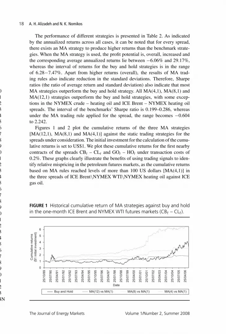
The performance of different strategies is presented in Table 2. As indicatedby the annualized returns across all cases, it can be noted that for every spread,there exists an MA strategy to produce higher returns than the benchmark strate-gies. When the MA strategy is used, the profit potential is, overall, increased andthe corresponding average annualized returns lie between −6.06% and 29.17%,whereas the interval of returns for the buy and hold strategies is in the rangeof 6.28−7.47%. Apart from higher returns (overall), the results of MA trad-ing rules also indicate reduction in the standard deviations. Therefore, Sharperatios (the ratio of average return and standard deviation) also indicate that mostMA strategies outperform the buy and hold strategy. All MA(4,1), MA(8,1) andMA(12,1) strategies outperform the buy and hold strategies, with some excep-tions in the NYMEX crude – heating oil and ICE Brent – NYMEX heating oilspreads. The interval of the benchmarks’ Sharpe ratio is 0.199–0.286, whereasunder the MA trading rule applied for the spread, the range becomes −0.604to 2.242.
Figures 1 and 2 plot the cumulative returns of the three MA strategies[MA(12,1), MA(8,1) and MA(4,1)] against the static trading strategies for thespreads under consideration. The initial investment for the calculation of the cumu-lative returns is set to US$1. We plot these cumulative returns for the first nearbycontracts of the spreads CBt – CLt and GOt – HOt under transaction costs of0.2%. These graphs clearly illustrate the benefits of using trading signals to iden-tify relative mispricing in the petroleum futures markets, as the cumulative returnsbased on MA rules reached levels of more than 100 US dollars [MA(4,1)] inthe three spreads of ICE Brent\NYMEX WTI\NYMEX heating oil against ICEgas oil.
FIGURE 1 Historical cumulative return of MA strategies against buy and holdin the one-month ICE Brent and NYMEX WTI futures markets (CBt – CLt ).
0
1
2
3
4
5
6
25/1
0/89
25/0
7/90
25/0
4/91
25/0
1/92
25/1
0/92
25/0
7/93
25/0
4/94
25/0
1/95
25/1
0/95
25/0
7/96
25/0
4/97
25/0
1/98
25/1
0/98
25/0
7/99
25/0
4/00
25/0
1/01
25/1
0/01
25/0
7/02
25/0
4/03
25/0
1/04
25/1
0/04
25/0
7/05
25/0
4/06
Buy and Hold MA(12) vs MA(1) MA(8) vs MA(1)
Date
Cum
ulat
ive
retu
rns
($1
initi
al in
vest
men
t)
MA(4) vs MA(1)
1234567891011121314151617181920212223242526272829303132333435363738394041424344N
The Journal of Energy Markets Volume 1/Number 2, Summer 2008

“EnerMarket: jem080307nm” — 2008/6/18 — 21:17 — page 19 — #17
Performance of statistical arbitrage in petroleum futures markets 19
FIGURE 2 Historical cumulative return of MA strategies against buy andhold in the one-month ICE Gas oil and NYMEX heating oil futures markets(GOt – HOt ).
0
20
40
60
80
100
120
140
25/1
0/89
25/0
7/90
25/0
4/91
25/0
1/92
25/1
0/92
25/0
7/93
25/0
4/94
25/0
1/95
25/1
0/95
25/0
7/96
25/0
4/97
25/0
1/98
25/1
0/98
25/0
7/99
25/0
4/00
25/0
1/01
25/1
0/01
25/0
7/02
25/0
4/03
25/0
1/04
25/1
0/04
25/0
7/05
25/0
4/06
Buy and Hold MA(12) vs MA(1) MA(8) vs MA(1) MA(4) vs MA(1)
Date
Cum
ulat
ive
retu
rns
($1
initi
al in
vest
men
t)
7 DATA SNOOPING AND THE STATIONARY BOOTSTRAP
The results in Section 6 are encouraging regarding the performance of our proposedtrading strategies. However, an important issue that arises when evaluating tradingrules is that of data snooping. According to Sullivan et al (1999) and White (2000),data snooping occurs when a data set is used more than once for data selection andinference purposes. In other words, using the same data set frequently for testingtrading strategies may increase the probability of having satisfactory results purelydue to chance or due to the use of posterior information rather than the superiorability of the trading strategies.
The method most commonly used in the literature to assess the performanceof trading strategies and test for data snooping is bootstrap. The bootstrap, intro-duced by Efron (1979), is a resampling method that uses the empirical distributionof the statistic of interest, rather than the theoretical distribution implied by thestatistical theory, to conduct statistical inference. The main advantage of bootstrapis that it can approximate the properties of the sampling distribution of the under-lying statistic even when such a distribution is not parametrically defined, or theunderlined statistic is complex and not easy to obtain. Bootstrap techniques havealso been used by Brock et al (1992), who test whether trading results from sometrading rules can be explained by time-series models, and Sullivan et al (1999),who use bootstrap to test the joint performance of several technical rules.
However, when ordinary bootstrap techniques are applied to serially dependentobservations, as in the case of petroleum and petroleum product futures prices, theresampled series will not retain the statistical properties of the original data set andyield inconsistent results and statistical inference (see Ruiz and Pascual (2002)).
1234567891011121314151617181920212223242526272829303132333435363738394041424344N
Research Paper www.thejournalofenergymarkets.com

“EnerMarket: jem080307nm” — 2008/6/18 — 21:17 — page 20 — #18
20 A. H. Alizadeh and N. K. Nomikos
In view of that, we employ the stationary bootstrap method of Politis and Romano(1994). This procedure is based on resampling blocks of random length, where thelength of each block follows a geometric distribution. This procedure generatesrandom samples that preserve the serial dependence property of the original seriesand are also stationary. This is important since our proposed trading strategy relieson the premise that the differentials of the futures prices under study are stationary;see Appendix for technical details.
Therefore, in order to assess the performance of our trading strategies, weuse the stationary bootstrap technique to regenerate random paths that futuresprices may have possibly followed over the sample period, while maintaining thedistributional properties of the original series. We then implement the proposedtrading strategies using the simulated prices’ series which, in turn, generate adistribution of trading statistics under the different trading rules. Therefore, ourapproach in using bootstrap is different from the previous literature in the sensethat we bootstrap to generate paths of the spread series and subsequently assessthe profitability of MA-based trading rules. This approach follows Alizadeh andNomikos (2006).
We start by bootstrapping the logdifference series. Then these bootstrappedseries are transformed back into levels to construct the spreads that are used totrigger buy and sell decisions based on the MA trading strategies. In implementingthese strategies, we consider 0.2% transaction costs. As benchmark models, wealso consider the buy and hold trading strategy in which one is always long ineither leg of the spread and, hence, benefits from a possible income irrespectiveof the level and fluctuation of the spread. Both the MA and the two buy and holdstrategies (two legs of the spread) are implemented for each one of the 1,000bootstrapped series, thus generating a series of empirical distributions of meanreturns and Sharpe ratios. Under the null hypothesis that a dynamic strategy is nobetter than a buy and hold strategy, or, equivalently, that there is no information orsignals in the original spread series, the profit from the MA strategies should beno better than the profit from the buy and hold strategies.
The results of the bootstrap simulations are reported in Table 2 in terms ofimprovement in Sharpe ratios. The mean annualized returns (obtained as the meanreturn from the trading strategies implemented on the 1,000 bootstrapped series)and average Sharpe ratio across the bootstrapped series are not presented heresince they are very similar to those observed in the empirical series under thesame trading rule. Furthermore, the comparative performance is also similar;for instance, the higher returns come from the three spreads that include ICEgas oil in the one leg, ie, ICE Brent\NYMEX WTI\NYMEX heating oil ver-sus ICE gas oil, whereas the worst performance is achieved by the four-monthNYMEX crude – heating oil spread for the MA(12,1) strategy. Overall, theMA-based trading rules seem to outperform the static investment tactics bothin terms of increasing average returns and in terms of the Sharpe ratios. Buy andhold oil futures strategies’ Sharpe ratios vary from 0.220 to 0.307. MA(12,1)-based Sharpe ratios lie between −0.782 and 1.807, MA(8,1) from −0.351 to
1234567891011121314151617181920212223242526272829303132333435363738394041424344N
The Journal of Energy Markets Volume 1/Number 2, Summer 2008

“EnerMarket: jem080307nm” — 2008/6/18 — 21:17 — page 21 — #19
Performance of statistical arbitrage in petroleum futures markets 21
2.281 and the MA(4,1) spread strategy has a better downside limit with Sharperatios in the range of 0.195–2.156. In all MA rules and maturities, the highestSharpe ratio is achieved by the ICE gas oil – NYMEX heating oil spread. Withthe exception of the MA(12,1)- and MA(8,1)-based strategies of the NYMEXcrude – heating oil spread and ICE Brent – NYMEX heating oil spread, allthe differences in the Sharpe ratios have a positive sign, denoting improve-ment. For example, the Sharpe ratios of the ICE gas oil – NYMEX heating oilspread reveal a more than eightfold increase compared with the buy and holdstrategies.
More formal statistical tests are conducted by testing whether the excess per-formance of the Sharpe ratio, based on the bootstrap simulations, is significantlydifferent from zero. More specifically, for each simulated series, we estimate theexcess Sharpe ratio of the MA trading strategy relative to the buy and hold strategy.We then construct the p-values for the tests in Table 2. These are simply calcu-lated as the ratio of frequency of occurrence of negative excess Sharpe ratios overthe total number of simulations (1,000 replications) and reflect significance level,for which the null hypothesis that there is no significant difference between theSharpe ratios can be rejected, using a one-tail test. Overall, these results indicatethat the MA strategies can provide significant increases in Sharpe ratios com-pared with the ordinary buy and hold strategies. More specifically, four out ofsix, one-month spreads achieve significantly higher Sharpe ratios compared withthe buy and hold strategy. The same is true for the two- and three-month case,whereas in the case of four-month spreads, the figure is reduced to three out of six.Overall, p-values provide additional support for the robustness of the superiorityof the MA trading strategies compared with buy and hold benchmarks. Signif-icantly higher Sharpe ratios at 1% significance level are achieved in the one-,two-, three- and four-month spreads of ICE Brent, NYMEX WTI and heatingoil against ICE gas oil for all MA strategies as well as the one-month MA(4,1)strategy for the ICE – NYMEX intercrude spread. Significance is also achievedat 10% significance level for the latter spread [MA(8,1) strategy] as well as forthe one- and two-month MA(4,1) strategy of NYMEX WTI – heating oil andfinally for the three-month MA(4,1) strategy of ICE Brent – NYMEX heatingoil spread.
Figures 3 and 4 plot the distributions of returns of three MA strategies[MA(12,1), MA(8,1) and MA(4,1)] against the static trading strategies using thebootstrap technique for the spreads under consideration. We plot these distribu-tions for the first nearby contracts of the spreads CBt – CLt and GOt – HOt , undertransaction costs of 0.2%. These graphs clearly illustrate the benefits of usingtrading signals to identify relative mispricing in the petroleum futures markets,as the distribution of simulated returns based on MA rules show relatively lowerdispersion, in all cases, and significant shifts to the right, in three out of six cases(the three spreads that include ICE gas oil).
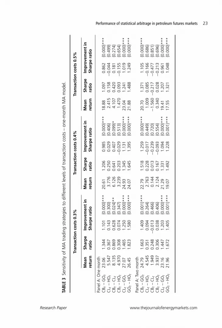
Provided that transaction costs are a significant trading cost factored in dynamictrading strategies and, also, given that these costs are subject to variations,
1234567891011121314151617181920212223242526272829303132333435363738394041424344N
Research Paper www.thejournalofenergymarkets.com

“EnerMarket: jem080307nm” — 2008/6/18 — 21:17 — page 22 — #20
22 A. H. Alizadeh and N. K. Nomikos
FIGURE 3 Bootstrapped distribution of returns of MA strategies against buyand hold in the one-month ICE Brent and NYMEX WTI futures markets(CBt – CLt ).
�0.2 �0.1 0.0 0.1Spread
0.2 0.3 0.40
5
10
15
Boo
tstra
pped
pro
babi
lity
dist
ribut
ion
of re
turn
s (%
)
20
25HOLD_STRATEGYMA(4) STRATEGYMA(8) STRATEGYMA(12) STRATEGY
FIGURE 4 Bootstrapped distribution of return of MA strategies against buy andhold in the one-month ICE gas oil and NYMEX heating oil futures markets(GOt – HOt ).
�0.16 �0.08 0.00 0.08 0.16 0.24 0.32 0.400.0
2.5
5.0
7.5
10.0
12.5
15.0HOLD_STRATEGYMA(4) STRATEGYMA(8) STRATEGYMA(12) STRATEGY
Spread
Boo
tstra
pped
pro
babi
lity
dist
ribut
ion
of re
turn
s (%
)
depending on the type of trader (eg, member or non-member) and the market(ie, United States, United Kingdom or both) involved, the performance of theMA trading strategies is tested, applying different sets of transaction costs in thebootstrap simulation, through sensitivity analysis.10 Table 3 reports the results
10 For economy of space, sensitivity analysis results present the outcome of the simulation of theone-month-based MA strategy that proved to be (overall) the best, under the 0.2% transactioncosts’ case. Another reason is that the specific strategy is expected to have the higher degree ofsensitivity to transaction costs, as the fastest MA [MA(4,1)] requires more frequent rebalancingof the portfolio. Sometimes, the number of trades increases to double compared with MA(12,1)or MA(8,1) strategy. Results, regarding the number of trades in both historical and bootstrapsimulations as well as sensitivity analysis, are available from the authors upon request.
1234567891011121314151617181920212223242526272829303132333435363738394041424344N
The Journal of Energy Markets Volume 1/Number 2, Summer 2008
“EnerMarket: jem080307nm” — 2008/6/18 — 21:17 — page 23 — #21
Performance of statistical arbitrage in petroleum futures markets 23
TABL
E3
Sens
itivi
tyof
MA
trad
ing
stra
tegi
esto
diff
eren
tle
vels
oftr
ansa
ctio
nco
sts
–on
e-m
onth
MA
mod
el.
Tran
sact
ion
cost
s0.
3%Tr
ansa
ctio
nco
sts
0.4%
Tran
sact
ion
cost
s0.
5%
Mea
nSh
arp
eIm
pro
vem
ent
inM
ean
Shar
pe
Imp
rove
men
tin
Mea
nSh
arp
eIm
pro
vem
ent
inre
turn
rati
oSh
arp
era
tio
retu
rnra
tio
Shar
pe
rati
ore
turn
rati
oSh
arp
era
tio
Pane
lA:O
nem
onth
CB t
–G
Ot
23.0
61.
344
1.10
1{0
.000
}***
20.6
11.
206
0.98
5{0
.000
}***
18.8
81.
097
0.86
2{0
.000
}***
CL t
–H
Ot
5.54
70.
367
0.14
3{0
.300
}3.
776
0.25
00.
029
{0.4
06}
2.41
50.
158
−0.0
44{0
.499
}C
B t–
CL t
8.13
50.
869
0.62
8{0
.024
}**
6.12
60.
641
0.40
7{0
.099
}*4.
107
0.42
00.
181
{0.2
74}
CB t
–H
Ot
4.97
00.
308
0.07
4{0
.347
}3.
239
0.20
3−0
.029
{0.5
13}
1.47
00.
093
−0.1
55{0
.654
}C
L t–
GO
t27
.07
1.46
51.
250
{0.0
00}*
**24
.93
1.34
51.
131
{0.0
00}*
**23
.04
1.24
11.
019
{0.0
00}*
**G
Ot
–H
Ot
26.4
51.
823
1.58
0{0
.000
}***
24.0
71.
645
1.39
5{0
.000
}***
21.8
81.
488
1.24
9{0
.000
}***
Pane
lA:T
wo
mon
thC
B t–
GO
t24
.79
1.66
31.
409
{0.0
01}*
**22
.79
1.51
81.
259
{0.0
00}*
**20
.70
1.37
11.
105
{0.0
00}*
**C
L t–
HO
t4.
545
0.35
10.
094
{0.2
64}
2.76
30.
228
−0.0
17{0
.449
}1.
009
0.08
5−0
.166
{0.6
86}
CB t
–C
L t1.
949
0.24
8−0
.013
{0.4
66}
0.14
40.
013
−0.2
39{0
.720
}−1
.560
−0.2
17−0
.477
{0.8
51}
CB t
–H
Ot
3.93
70.
306
0.03
8{0
.406
}2.
124
0.16
7−0
.093
{0.5
54}
0.34
00.
028
−0.2
13{0
.696
}C
L t–
GO
t23
.16
1.44
71.
203
{0.0
00}*
**21
.29
1.33
11.
094
{0.0
00}*
**19
.41
1.20
70.
961
{0.0
00}*
**G
Ot
–H
Ot
21.9
61.
672
1.40
5{0
.001
}***
19.0
71.
492
1.22
8{0
.001
}***
17.5
51.
321
1.04
8{0
.000
}***
1234567891011121314151617181920212223242526272829303132333435363738394041424344N
Research Paper www.thejournalofenergymarkets.com

“EnerMarket: jem080307nm” — 2008/6/18 — 21:17 — page 24 — #22
24 A. H. Alizadeh and N. K. Nomikos
TABL
E3
Con
tinue
d. Tran
sact
ion
cost
s0.
3%Tr
ansa
ctio
nco
sts
0.4%
Tran
sact
ion
cost
s0.
5%
Mea
nSh
arp
eIm
pro
vem
ent
inM
ean
Shar
pe
Imp
rove
men
tin
Mea
nSh
arp
eIm
pro
vem
ent
inre
turn
rati
oSh
arp
era
tio
retu
rnra
tio
Shar
pe
rati
ore
turn
rati
oSh
arp
era
tio
Pane
lC:T
hree
mon
thC
B t–
GO
t25
.89
1.83
41.
550
{0.0
00}*
**23
.57
1.67
61.
383
{0.0
00}*
**21
.79
1.53
31.
241
{0.0
02}*
**C
L t–
HO
t3.
108
0.30
10.
016
{0.4
09}
1.24
30.
133
−0.1
47{0
.643
}−0
.050
−0.0
54−0
.324
{0.8
06}
CB t
–C
L t1.
510
0.19
2−0
.084
{0.5
45}
−0.4
33−0
.084
−0.3
74{0
.756
}−2
.519
−0.3
69−0
.653
{0.8
60}
CB t
–H
Ot
6.60
70.
586
0.29
5{0
.155
}4.
754
0.42
40.
154
{0.3
02}
3.01
10.
269
−0.0
070.
458
CL t
–G
Ot
24.4
31.
674
1.41
7{0
.000
}***
22.3
41.
525
1.26
3{0
.000
}***
20.1
21.
373
1.10
0{0
.000
}***
GO
t–
HO
t24
.35
1.97
41.
684
{0.0
00}*
**21
.87
1.76
71.
486
{0.0
00}*
**19
.78
1.58
21.
297
{0.0
00}*
**
Pane
lD:F
our
mon
thC
B t–
GO
t24
.34
1.80
21.
497
{0.0
00}*
**22
.06
1.63
91.
330
{0.0
00}*
**19
.92
1.47
11.
167
{0.0
00}*
**C
L t–
HO
t0.
001
0.00
2−0
.280
{0.7
37}
−1.6
71−0
.177
−0.4
64{0
.834
}−3
.436
−0.3
60−0
.650
{0.8
75}
CB t
–C
L t2.
435
0.32
40.
015
{0.4
51}
0.45
20.
034
−0.2
62{0
.680
}−1
.532
−0.2
49−0
.557
{0.8
25}
CB t
–H
Ot
3.63
10.
342
0.04
0{0
.407
}1.
938
0.18
5−0
.109
{0.5
69}
0.27
00.
026
−0.2
72{0
.705
}C
L t–
GO
t23
.48
1.70
41.
409
{0.0
00}*
**21
.21
1.52
51.
234
{0.0
01}*
**19
.10
1.37
21.
088
{0.0
01}*
**G
Ot
–H
Ot
23.4
11.
972
1.65
8{0
.000
}***
21.2
71.
783
1.50
4{0
.001
}***
18.7
81.
567
1.24
7{0
.000
}***
See
note
sin
Tabl
e2.
1234567891011121314151617181920212223242526272829303132333435363738394041424344N
The Journal of Energy Markets Volume 1/Number 2, Summer 2008

“EnerMarket: jem080307nm” — 2008/6/18 — 21:17 — page 25 — #23
Performance of statistical arbitrage in petroleum futures markets 25
for transaction costs in the range of 0.3%, 0.4% and 0.5%, respectively, for all thematurities of each spread trading strategies, based on the fastest MA.
One first important observation is that the three out of the six spreads, namelyCBt – GOt , CLt – GOt and GOt – HOt , produce significantly higher (at 1% signif-icance level) Sharpe ratios than the buy and hold strategies, even in the high zoneof 0.5% transaction costs. The annualized returns are in the range of 18.9–23.0%,which means more than twofold to fourfold increase compared with the buy andhold strategies. This implies that in the specific three spread markets, the mean-reverting tendencies, as implied by the fair value of the spread (estimated usingJohansen (1988) cointegration procedure), are not fully impounded in the expec-tations of the market and abnormal excess returns become possible. Regarding theother three spreads, CLt – HOt , CBt – CLt and CBt – HOt , relative mispricingis also discernible, subject to transaction costs. When transaction costs are 0.3%and 0.4% significantly higher Sharpe ratios are also achieved by the one-monthintercrude CBt – CLt spread.
Finally, one vital question that arises is why some spreads perform better thanothers and how we can identify these trading opportunities. Although petroleumfutures prices move together in the long run, as indicated byλtrace andλmax statisticsof Johansen (1988) cointegration tests (Table 1), they tend to show a differentbehavior in the short run. Long-run comovements are due to the fact that theseprices are driven by the same underlying factor, which are the conditions prevailingin the world oil markets. Highly correlated assets are possible to generate tradingopportunities by simultaneously taking opposite positions in these assets and profitfrom the divergence or convergence in prices. Divergence of futures prices occursmainly in the short run and can be attributed to seasonal factors, changes in regionalsupply/demand and flow of new information. This pattern is also shown in Figures 5and 6, where the 52-week rolling correlation is plotted. The strength of these short-run comovements is determined by the correlation coefficient of changes in futuresprices. High correlation between the legs of the pair in the long run, together withthe relatively lower correlation in the short run, are two of the essential indicatorsone should examine before initiating a spread trading strategy, since these measuresprovide information on the frequency of divergence from the aforementioned long-run relationship. Another important indicator is the level of volatility of both pricesand returns, which determines the degree of divergence from the aforementionedlong-run relationship. Normally, we would expect the higher the correlation in thelong run and the lower the correlation in the short run to produce the best possibleoutcome. However, the volatility effect cannot be neglected because the individualrelationship between correlation and standard deviation is market specific andindicates that it would be more appropriate to adjust these coefficients in order toget a relative measure, subject to the levels of volatility both in the longer and inthe shorter term. This is based on the fact that in spite of the theoretical negativerelationship between correlation and volatility (that is the higher the correlation,the lower the volatility), the strength of this relationship, the “steepness” of theslope between these two measures and the existence or not of non-linearities are
1234567891011121314151617181920212223242526272829303132333435363738394041424344N
Research Paper www.thejournalofenergymarkets.com

“EnerMarket: jem080307nm” — 2008/6/18 — 21:17 — page 26 — #24
26 A. H. Alizadeh and N. K. Nomikos
FIGURE 5 Time-varying correlation in levels and first differences between theone-month ICE Brent and NYMEX WTI futures markets (CBt − CLt ).
0
0.2
0.4
0.6
His
toric
al c
orre
latio
n(5
2-w
eek
rolli
ng w
indo
w)
0.8
1
07/0
3/90
02/1
2/90
29/0
8/91
25/0
5/92
19/0
2/93
16/1
1/93
13/0
8/94
10/0
5/95
04/0
2/96
31/1
0/96
28/0
7/97
24/0
4/98
19/0
1/99
16/1
0/99
12/0
7/00
08/0
4/01
03/0
1/02
30/0
9/02
27/0
6/03
23/0
3/04
18/1
2/04
14/0
9/05
11/0
6/06
Correlation in levels Correletion in first difference
Date
FIGURE 6 Time-varying correlation in levels and first differences between theone-month ICE gas oil and NYMEX heating oil futures markets (GOt − HOt ).
0
0.2
0.4
0.6
0.8
1
07/0
3/90
02/1
2/90
29/0
8/91
25/0
5/92
19/0
2/93
16/1
1/93
13/0
8/94
10/0
5/95
04/0
2/96
31/1
0/96
28/0
7/97
24/0
4/98
19/0
1/99
16/1
0/99
12/0
7/00
08/0
4/01
03/0
1/02
30/0
9/02
27/0
6/03
23/0
3/04
18/1
2/04
14/0
9/05
11/0
6/06
Correlation in levels Correletion in first difference
His
toric
al c
orre
latio
n(5
2-w
eek
rolli
ng w
indo
w)
Date
of paramount importance. Hence, long- and short-run correlation justifies pairstrading and long- and short-run volatility includes information on the potentialprofitability of the spread under study, on the grounds that as the spread deviatesfrom the long-run equilibrium, the probability of convergence is increased alongwith the probability of achieving higher profits. Table 4 reports the followingcorrelation volatility ratio:
CVR = ρF1,F2/σ(F1−F2)
ρdF1,dF2/σ(dF1−dF2)
(2)
1234567891011121314151617181920212223242526272829303132333435363738394041424344N
The Journal of Energy Markets Volume 1/Number 2, Summer 2008

“EnerMarket: jem080307nm” — 2008/6/18 — 21:17 — page 27 — #25
Performance of statistical arbitrage in petroleum futures markets 27
TABL
E4
Long
-an
dsh
ort-
term
unco
nditi
onal
corr
elat
ions
betw
een
petr
oleu
mfu
ture
s.
Thre
e-m
on
thst
rate
gy
Two
-mo
nth
stra
teg
yO
ne-
mo
nth
stra
teg
yC
VR
CV
R(M
A12
vsM
A1)
(MA
4vs
MA
1)(M
A12
vsM
A1)
Co
rrel
atio
nSt
and
ard
Dev
iati
on
rati
ora
nk
Shar
pe
Ran
kSh
arp
eR
ank
Shar
pe
Ran
kLe
vels
Ret
urn
sSp
read
Ch
ang
esin
rati
ora
tio
rati
osp
read
Pane
lA:O
nem
onth
CB t
–G
Ot
1.00
63
1.14
23
1.43
53
0.99
070.
8316
0.41
70.
184
0.52
83
CL t
–H
Ot
0.29
06
0.37
25
0.56
15
0.99
110.
8774
0.39
80.
158
0.44
96
CB t
–C
L t0.
386
40.
703
41.
184
40.
9983
0.95
560.
210
0.09
70.
485
4C
B t–
HO
t0.
361
50.
272
60.
426
60.
9911
0.86
060.
409
0.16
90.
475
5C
L t–
GO
t1.
027
21.
267
21.
571
20.
9890
0.80
640.
444
0.19
80.
549
2G
Ot
–H
Ot
1.51
31
1.80
41
1.95
01
0.99
720.
8741
0.22
40.
158
0.80
11
Pane
lB:T
wo
mon
thC
B t–
GO
t1.
202
21.
332
21.
800
20.
9922
0.85
290.
383
0.16
10.
488
3C
L t–
HO
t−0
.117
60.
024
60.
560
50.
9926
0.90
900.
360
0.12
50.
379
6C
B t–
CL t
0.39
75
0.47
85
0.57
24
0.99
880.
9644
0.18
50.
081
0.45
04
CB t
–H
Ot
0.54
94
0.61
04
0.54
66
0.99
290.
8991
0.36
70.
134
0.40
25
CL t
–G
Ot
1.11
73
1.23
53
1.59
03
0.99
090.
8300
0.40
00.
171
0.51
02
GO
t–
HO
t1.
886
12.
011
11.
840
10.
9979
0.88
400.
193
0.14
10.
825
1 1234567891011121314151617181920212223242526272829303132333435363738394041424344N
Research Paper www.thejournalofenergymarkets.com
“EnerMarket: jem080307nm” — 2008/6/18 — 21:17 — page 28 — #26
28 A. H. Alizadeh and N. K. Nomikos
TABL
E4
Con
tinue
d.
Thre
e-m
on
thst
rate
gy
Two
-mo
nth
stra
teg
yO
ne-
mo
nth
stra
teg
yC
VR
CV
R(M
A12
vsM
A1)
(MA
4vs
MA
1)(M
A12
vsM
A1)
Co
rrel
atio
nSt
and
ard
Dev
iati
on
rati
ora
nk
Shar
pe
Ran
kSh
arp
eR
ank
Shar
pe
Ran
kLe
vels
Ret
urn
sSp
read
Ch
ang
esin
rati
ora
tio
rati
osp
read
Pane
lC:T
hree
mon
thC
B t–
GO
t1.
370
21.
689
22.
015
20.
9920
0.85
160.
361
0.14
90.
482
3C
L t–
HO
t−0
.400
6−0
.283
60.
523
60.
9937
0.92
300.
329
0.10
80.
352
6C
B t–
CL t
0.46
54
0.43
84
0.58
95
0.99
910.
9635
0.17
30.
077
0.46
04
CB t
–H
Ot
0.16
45
0.31
75
0.88
54
0.99
400.
9112
0.34
10.
118
0.37
85
CL t
–G
Ot
1.24
63
1.42
63
1.77
93
0.99
130.
8344
0.36
50.
153
0.49
92
GO
t–
HO
t2.
106
12.
242
12.
160
10.
9964
0.87
490.
182
0.13
60.
851
1
Pane
lD:F
our
mon
thC
B t–
GO
t1.
509
21.
747
21.
983
20.
9939
0.84
320.
345
0.14
80.
506
3C
L t–
HO
t−0
.604
6−0
.358
60.
230
60.
9945
0.92
320.
307
0.10
10.
356
6C
B t–
CL t
0.50
14
0.64
14
0.78
94
0.99
910.
9565
0.17
00.
079
0.48
64
CB t
–H
Ot
0.08
25
0.15
75
0.61
75
0.99
450.
9102
0.32
90.
113
0.37
55
CL t
–G
Ot
1.35
53
1.51
33
1.77
03
0.99
330.
8294
0.33
80.
150
0.53
12
GO
t–
HO
t2.
009
12.
090
12.
129
10.
9980
0.87
500.
182
0.13
10.
795
1
Rank
ing
isca
rrie
dou
tby
rank
ing
the
perf
orm
ance
ofth
esp
read
sun
der
stud
y,ac
cord
ing
toth
eir
hist
oric
alSh
arpe
ratio
s.Th
era
tiois
calc
ulat
edas
inEq
uatio
n(2
).
1234567891011121314151617181920212223242526272829303132333435363738394041424344N
The Journal of Energy Markets Volume 1/Number 2, Summer 2008

“EnerMarket: jem080307nm” — 2008/6/18 — 21:17 — page 29 — #27
Performance of statistical arbitrage in petroleum futures markets 29
where ρF1,F2 and ρdF1,dF2 are the loglevel (long run) and logchange (short run)correlations between the legs of the spread, ie, F1 and F2, respectively. σ(F1−F2)
is the variance (long run) of a portfolio consisting of F1 and F2 and σ(dF1−dF2)
is the variance (short run) of changes in the spread series. As it can be seen inTable 4, this ratio is able to distinguish the most profitable petroleum spreads fromthe unprofitable ones. However, this ratio is only a relative measure that can pro-vide a broad indicator since a spread trading strategy is not considered successfulunless transaction costs are covered and the benchmark strategy is outperformed.Consequently, this ratio can be used only in combination with fundamental andtechnical analyses. For instance, the two spreads of CBt – HOt and GOt – HOt
display similar correlation dynamics both in the long (0.991 vs 0.997) and in theshort run (0.861 vs 0.874). However, for the first spread, the bootstrap exerciseresulted in annualized returns not more than 7% and 3% under 0.3% and 0.5%transaction costs, respectively. On the other hand, the GOt – HOt , spread realizedreturns in excess of 17.5%, in the conservative case of 0.5% transaction costs.This is an example of the effect of volatility on the aforementioned ratio. CBt –HOt has significantly greater volatility than GOt – HOt in the long run, whereasfor the changes in the spread (short run), the volatility ratio is reduced and isnot significantly different (at 5% significance level)11 for the one- and two-monthspread, resulting a stronger correlation in the long run for the GOt – HOt spread.Time-varying correlation based on a 52-week rolling window indicated that inthe case of one-month CBt – HOt , the minimum value was 0.41, whereas for theGOt – HOt spread the same figure is 0.88. This is also evident in Table 1 where coin-tegration is stronger in the GOt – HOt pair, according to λtrace and λmax statistics.On the other hand, in the case of the CBt – HOt , speed of adjustment coefficientsare of less magnitude, indicating lower responsiveness to the differential, and inthe three- and four-month case, there is no causality at 5% significance level.
8 CONCLUSIONS
In this study, we tested the performance of MA trading strategies in the petroleumfutures markets. In particular, we utilized linkages between different pairs ofpetroleum futures and devised strategies to identify timing for statistical arbitrage.Error correction models were employed to discover the fundamental drivers of themarket and causality direction. Using the cointegration relationship, we furtherdeveloped a trading strategy that is based on the deviation of oil futures spreadsfrom their long-run mean, combining both the NYMEX and the ICE markets. Theturning points are identified using MA trading rules, which are used as indicatorsfor buy and sell opportunities. Simple MA trading strategies proved to be able to
11 F-tests of equality of variance for the a) spread and b) changes in spread resulted in thefollowing statistics (p-values): a) One-month: 3.327 (0.000), two-month: 3.603 (0.000), three-month: 3.543 (0.000) and four-month: 3.081 (0.000) b) One-month: 1.144 (0.045), two-month:1.119 (0.093), three-month: 1.315 (0.000) and four-month: 1.357 (0.000).
1234567891011121314151617181920212223242526272829303132333435363738394041424344N
Research Paper www.thejournalofenergymarkets.com

“EnerMarket: jem080307nm” — 2008/6/18 — 21:17 — page 30 — #28
30 A. H. Alizadeh and N. K. Nomikos
improve Sharpe ratios and provided evidence that statistical arbitrage opportuni-ties are present in all the combinations of petroleum futures spreads under study,subject to transaction costs. Allowing for variation in transaction costs, maturi-ties of futures prices and MA windows, three out of six spreads proved to bevery profitable having realized annualized returns of 18.2–30.0%. Namely, ICEBrent versus gas oil, NYMEX WTI versus ICE gas oil and NYMEX heating oilversus ICE gas oil achieved annualized returns of 17–29%, after accounting fordata snooping; this corresponds to Sharpe ratios from 1.00 to 2.28 (3–10 timesimprovement compared with the buy and hold strategies). Less profitable, yet sig-nificant improvement from the employment of technical trading rules, proved tobe the one-month intercrude differential.
By and large, our results revealed that the relationship between petroleumfutures prices can be used for investment timing, and investors can benefit fromtechnical trading rules, had these rules been based on sound fundamental argu-ments. The high volatility and high long-run correlation of petroleum futuresrenders the use of spread trading strategies, where relatively lower-margin require-ments and risk exposure along with netting effects can offset the high bid–askspreads. The rationale behind spread trading is based on the mean-reverting prop-erties of the differential, which are described by the time aggregation of bothcorrelation (which justifies pairs trading) and volatility (which includes informa-tion on the potential profitability of the spread). Hence, the long- and short-runcorrelation and volatility dynamics can provide a good indicator whether statisticalarbitrage opportunities are open. Overall, the results indicate that simple MA indi-cators are able to exploit statistical arbitrage opportunities among futures prices,and by using such indicators, market agents may be able to obtain superior gains,measured in terms of annualized returns and increase in Sharpe ratios.
APPENDIX
Here, we present the algorithm that is used to implement the stationary bootstrap re-sampling technique of Politis and Romano (1994). The description of the algorithmhere follows from Appendix C of Sullivan et al (1999).
The stationary bootstrap is calculated as follows: given the original sample of Tobservations, X(t), t = {1, . . . , T}, we start by selecting a “smoothing parameter”,q = qT , 0 < qT ≤ 1, TqT → ∞ as T → ∞, and from the bootstrapped series,X(t)*, as follows:
1) At t = 1, select X(1)* at random, independently and uniformly from{X(1), . . . , X(t)}. Say for instance that X(1)* is selected to be the Jthobservation in the original series, X(1)* = X(J), where 1 ≤ J ≤ T .
2) Increment t by 1. If t > T , then stop. Otherwise draw a standard uniformrandom variable U independently of all other random variables.
1234567891011121314151617181920212223242526272829303132333435363738394041424344N
The Journal of Energy Markets Volume 1/Number 2, Summer 2008

“EnerMarket: jem080307nm” — 2008/6/18 — 21:17 — page 31 — #29
Performance of statistical arbitrage in petroleum futures markets 31
(a) If U < q, then select X(2)* at random, independently from{X(1), . . . , X(T)}.
(b) If U > q, then expand the block by setting X(2)* = X(J + 1), so thatX(2)* is the next observation in the original series following X(J). IfJ + 1 > T , then reset J + 1 to 1, so that the block continues from thefinal observation in the sample.
3) Repeat Step 2 until we reach X(T)*.4) Repeat Steps 1–3 1,000 times.
Therefore, the stationary bootstrap resamples blocks of varying length from theoriginal data, where the block length follows a geometric distribution, with meanblock length 1/q. In general, given that X(t)* is determined by the Jth observationX(J), in the original series, then X(t + 1)* will be equal to the next observation inthe block X(J + 1) with probability 1–q and picked at random from the originalobservations with probability q. Regarding the choice of q, a large value of q isappropriate for data with little dependence, and a smaller value of q is appropriatefor data that exhibit serial dependence. The value of q chosen in our experimentsis 0.1, corresponding to a mean block length of 10. This follows other studies inthe literature, most notably Sullivan et al (1999). Furthermore, we also performsensitivity tests with different values of q and find that the results presented in thissection are not sensitive to the choice of q.
REFERENCES
Alizadeh, A. H., and Nomikos, N. (2004). The cost of carry, causality and arbitrage betweenoil futures and tanker freight markets. Transportation Research, Part E 40, 297–316.
Alizadeh, A. H., and Nomikos, N. (2006). Investment timing and trading strategies in thesale and purchase market for ships. Transportation Research, Part B 41(1), 126–143.
Brock, W., Lakonishok, J., and LeBaron, B. (1992). Simple technical trading rules and thestochastic properties of stock returns. Journal of Finance 47(5), 1731–1764.
Cheung, Y., and Lai, K. (1993). A cointegration test for oil futures market efficiency. TheJournal of Futures Markets 13, 933–941.
Crowder, W., and Hamed, A. (1993). A cointegration test for oil futures market efficiency.The Journal of Futures Markets 13, 933–941.
Dunis, C. L., Laws, J., and Evans, B. (2006a). Trading futures spreads: an application ofcorrelation and threshold filters. Applied Financial Economics 16, 903–914.
Dunis, C. L., Laws, J., and Evans, B. (2006b). Trading futures spreads portfolios:application of higher order and recurrent networks. Working Paper, Centre for Interna-tional Banking, Economics and Finance (CIBEF) and Liverpool John Moores University(JMU), UK.
Efron, B. (1979). Bootstrap methods: another look at the jackknife. Annals of Statistics 7,1–26.
Emery, G. W., and Liu, Q. (2002). An analysis of the relationship between electricity andnatural-gas futures prices. The Journal of Futures Markets 22, 95–122.
1234567891011121314151617181920212223242526272829303132333435363738394041424344N
Research Paper www.thejournalofenergymarkets.com

“EnerMarket: jem080307nm” — 2008/6/18 — 21:17 — page 32 — #30
32 A. H. Alizadeh and N. K. Nomikos
Engle, R. F., and Granger, C. W. (1987). Cointegration and error correction: representation,estimation, and testing. Econometrica 55, 251–276.
Ewing, B., and Harter, C. (2000). Co-movements of Alaska North Slope and UK Brentcrude oil prices. Applied Economic Letters 7, 555–558.
Girma, P. B., and Paulson, A. S. (1999). Risk arbitrage opportunities in petroleum futuresspreads. The Journal of Futures Markets 19, 931–955.
Gonzalo, J. (1994). Five alternative methods of estimating long-run equilibrium relation-ships. Econometrica 60, 203–233.
Granger, C. (1969). Investigating causal relations by econometric models and cross-spectralmethods. Econometrica 37, 424–438.
Granger, C. (1986). Developments in the study of cointegrated variables. Oxford Bulletinof Economics and Statistics 48, 213–227.
Haigh, M. S., and Holt, M. T. (2002). Crack spread hedging: accounting for time-varyingvolatility spillovers in the energy futures markets. Journal of Applied Econometrics 17,269–289.
Johansen, S. (1988). Statistical analysis of cointegrating vectors. Journal of EconomicDynamics and Control 12, 231–254.
Johansen, S. (1991). Estimation and hypothesis testing of cointegrating vectors in Gaussianvector autoregressive models. Econometrica 59, 1551–1558.
Johansen, S., and Juselius, K. (1991). Maximum likelihood estimation and inferenceon cointegration – with applications to the demand for money. Oxford Bulletin ofEconomics and Statistics 52, 169–211.
Johnson, R. L., Zulauf, C. R., Irwin, S. H., and Gerlow, M. E. (1991). The soybean complexspread: an examination of market efficiency from the viewpoint of production process.The Journal of Futures Markets 1, 565–596.
Lee, T., and Tse, Y. (1996). Tests with conditional heteroscedasticity. Journal of Economet-rics 73, 401–410.
Lin, X. S., and Tamvakis, M. (2001). Spillover effects in energy futures markets. EnergyEconomics 23, 43–56.
Liu, Q. (2005). Price relations among hog, corn, and soybean meal futures. The Journal ofFutures Markets 25, 491–514.
Milonas, N., and Henker, T. (2001). Price spread and convenience yield behaviour in theinternational crude oil market. Applied Financial Economics 11, 23–26.
Newey, W., and West, K. (1987). A simple positive semi-definite, heteroscedasticity andautocorrelation consistent covariance matrix. Econometrica 55, 703–708.
Osterwald-Lenum, M. (1992). A note with the quantiles of the asymptotic distribution ofthe ML cointegration rank test statistics. Oxford Bulletin of Economics and Statistics 54,461–472.
Poitras, G., and Teoh, A. (2003). The crack spread: day trading the oil futures complex.Derivatives Use, Trading & Regulation 9, 102–116.
Politis, D. N., and Romano, J. P. (1994). The stationary bootstrap. Journal of the AmericanStatistical Association 89(428), 1303–1314.
Ruiz, E., and Pascual, L. (2002). Bootstrapping financial time series. Journal of EconomicSurveys 16, 271–300.
Samuelson, P. A. (1965). Proof that properly anticipated prices fluctuate randomly.Industrial Management Review 6, 41–63.
1234567891011121314151617181920212223242526272829303132333435363738394041424344N
The Journal of Energy Markets Volume 1/Number 2, Summer 2008

“EnerMarket: jem080307nm” — 2008/6/18 — 21:17 — page 33 — #31
Performance of statistical arbitrage in petroleum futures markets 33
Schwarz, G. (1978). Estimating the dimension of a model. Annals of Statistics 6, 461–464.
Silvapulle, P., and Moosa, I. (1999). The relationship between spot and futures prices:evidence from the crude oil market. The Journal of Futures Markets 19, 175–193.
Sullivan, R., Timmermann, A., and White, H. (1999). Data-snooping, technical trading ruleperformance, and the bootstrap. Journal of Finance 54(5), 1647–1691.
Wahab M., Cohn, R., and Lashgari, M. (1994). The gold–silver spread: integration, coin-tegration, predictability, and ex-ante arbitrage. The Journal of Futures Markets 14,709–756.
White, H. (2000). A reality check for data snooping. Econometrica 68, 1097–1126.
1234567891011121314151617181920212223242526272829303132333435363738394041424344N
Research Paper www.thejournalofenergymarkets.com

“EnerMarket: jem080307nm” — 2008/6/18 — 21:17 — page 34 — #32


