מאמריםמאמריםמאמריםמאמרים סדרתסדרתסדרתסדרת DISCUSSION PAPER SERIES

31905 חיפה ,הכרמל הר ,לכלכלה החוג ,חיפה אוניברסיטת University of Haifa, Department of Economics, Mt. Carmel, Haifa 31905 Israel

http://hevra.haifa.ac.il/econ/index.html

Sticky Prices and Sequential Trade

Benjamin Eden

Discussion Paper No. 01-05 July 2001

STICKY PRICES AND SEQUENTIAL TRADE

Benjamin Eden*

The University of Haifa

July 2001

I consider a cash-in-advance model in which agents arrive at the

market-place sequentially and choose goods according to McFadden's

random utility maximization model. I allow for price dispersion and a

two stage production process to get a positive relationship between

money and output. It is argued that a single-sticky-price model does not

deliver a monotonic relationship between money and output. The paper

thus makes a connection between the sticky-price literature and the

uncertain and sequential trade model.

JEL Classification numbers: E000, E300, E400.

Mailing address: Department of Economics, The University of Haifa, Haifa

31905, Israel.

E-mail: b.eden@econ.haifa.ac.il

2

1. INTRODUCTION

Sticky price models attribute the short run real effects of money

to the presence of price rigidities. It is typically assumed that (a)

prices do not adjust immediately to changes in the money supply and (b)

there is a commitment on the part of the firm to supply any quantity

demanded at the not fully adjusted prices.

The failure to fully adjust all prices to changes in the money

supply is often rationalized by the existence of fixed menu type cost

for changing nominal prices. Akerlof and Yellen (1985) and Blanchard and

Kiyotaki (1987) show that even when these fixed menu costs are small

they can cause large aggregate effects in a monopolistically competitive

environment.

The second assumption about the commitment of firms to supply any

quantity demanded has received less attention. Here I show that once

this assumption is relaxed, we may get a negative rather than a positive

relationship between money and output. This is shown in a

monopolistically competitive, cash-in-advance environment in which

buyers arrive at the market-place sequentially and choose a single brand

according to McFadden's random utility maximization model. The reason

for this somewhat surprising result is in the assumption that money

earned today is spent in the next period. Therefore, when a seller

observes a high money supply in the current period he expects a high

next period price level and a low real wage.

To overcome this difficulty I assume a two stage production

process and allow for many prices. In equilibrium sellers know exactly

for which realizations of the money supply they will satisfy demand. We

3

may therefore think of sellers as making a contingent demand satisfying

commitments. This type of demand satisfying behavior is rather

realistic. Stores often hit a capacity constraint and do not satisfy the

entire demand. They may also require buyers who arrive "late" to pay a

higher price. For example, a store may declare an item on "sale" and

commits to satisfy demand when the money supply is low. If the money

supply is high some buyers will not be able to find the item at the

sale-price and will have to buy it at the higher list-price. It may be

argued that the proposed model is more realistic than the single-sticky-

price model. More importantly, it yields an unambiguous positive

relationship between money and output.

The proposed model is a version of the uncertain and sequential

trading (UST) model in Eden (1994), Lucas and Woodford (1994), Bental

and Eden (1996), Woodford (1996) and Williamson (1996). In previous UST

models buyers who arrive at the market-place can see all supply offers

and buy at the cheapest available offer. In equilibrium sellers face a

tradeoff between the price and the probability of making a sale: a

seller who quotes a high price will make sale with low probability. The

fraction of output sold at a given price is therefore zero or unity.

This aspect has been criticized as unrealistic and more importantly it

poses a difficulty in applying the model to explain micro data (see,

Eden [forthcoming]). Here buyers do not always buy at the cheapest

available price and therefore in equilibrium some quantity of the more

expensive goods will always be sold. The tradeoff that arises in

equilibrium is between the average fraction of output sold and the price

rather than between the probability of making a sale and the price.

4

2. A STICKY PRICE MODEL

I consider a cash-in-advance model in which the typical

household is a worker/shopper pair. To simplify, I assume that the

single period utility function of the representative household is given

by c - v(L) where c denotes consumption and L denotes the labor input

supplied by the worker. The cost function v( ) has the standard

properties (v' > 0 and v'' > 0 everywhere). The household's discount

factor is given by 0 < β < 1. I use the beginning of the period money

supply (per household) as the unit of account and call it a normalized

dollar.1

At the beginning of the period the household starts with m

normalized dollars (in equilibrium m = 1) and gets a transfer of x

normalized dollars, where -1 ≤ x ≤ ∞ is the random rate of change in

the money supply. It is assumed that x is i.i.d with a density function

φ(x).

There is a large number (n) of households. Each worker produces a

different brand of the consumption good using a constant returns to

scale technology: One unit of output per unit of labor. The typical

worker first chooses his price. He then observes the money supply shock

x and then chooses output.

Buyers arrive sequentially and in equilibrium each spends 1 + x

normalized dollars on a single brand. I follow McFadden (2000) random

1 Thus, I divide all nominal magnitudes by the pre-transfer money

supply.

5

utility maximization model and assume that when n brands are available

the probability of choosing brand i is:

(1) Prob(i) = w i/Σnk=1 w

k,

where w i = exp(bZ

i), Z

i is a vector of attributes of brand i and b is a

vector of parameters.

I start from the case in which the only relevant attribute of a

brand is its relative price:

(2) w i = exp[α(p/p i)],

where p i is the price of brand i and p is the average price of all other

brands. It will be shown that under (2) the demand for brand i is

similar to what one gets when employing the Dixit-Stiglitz (1977)

utility function, which is more common in the macro literature. Here I

use the random utility maximization model because of the possibility to

introduce non-price competition. This will be attempted later.

Assuming that all other sellers quote the price p and that all the

n alternatives are available, the probability that the buyer will buy

brand i at the price p i is (approximately)

2:

(3) exp[α(p/p i)]/n[exp(α)].

2 The exact expression is: exp[α(p/p i)]/{(n-1)[exp(α)] + exp[α(p/p i)]}.

This is equal to (3) when n is large.

6

Note that when p i = p, the probability that the buyer will choose brand

i is 1/n. When p i > p the probability of choosing brand i is less than

1/n but is greater than zero. This is the monopolistic competition

aspect of the environment.

Seller i expects that other sellers will satisfy demand when

x ≤ ζ, where ζ is a cut-off parameter that will be determined in

equilibrium. Therefore when he observes x ≤ ζ, he assigns the

probability (3) to the event that a buyer will choose his product. He

can then choose whether to satisfy demand or not.

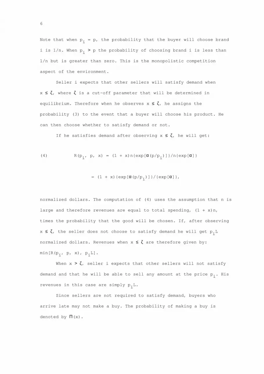
If he satisfies demand after observing x ≤ ζ, he will get:

(4) R(p i, p, x) = (1 + x)n{exp[α(p/p i)]}/n{exp[α]}

= (1 + x){exp[α(p/p i)]}/{exp[α]},

normalized dollars. The computation of (4) uses the assumption that n is

large and therefore revenues are equal to total spending, (1 + x)n,

times the probability that the good will be chosen. If, after observing

x ≤ ζ, the seller does not choose to satisfy demand he will get p iL

normalized dollars. Revenues when x ≤ ζ are therefore given by:

min[R(p i, p, x), p

iL].

When x > ζ, seller i expects that other sellers will not satisfy

demand and that he will be able to sell any amount at the price p i. His

revenues in this case are simply p iL.

Since sellers are not required to satisfy demand, buyers who

arrive late may not make a buy. The probability of making a buy is

denoted by Π(x).

7

Because of symmetry all sellers face the same revenue functions

and the same maximization problem. Labor is supplied to create money

that will be spent in the next period. To set the labor choice problem,

I use V(m) to denote the maximum expected utility that a household can

obtain when it starts the period with m normalized dollars. This value

function will soon be defined by a Bellman equation.

A seller who quoted the price p i and observes that other sellers

have quoted the price p and x ≤ ζ will choose labor by solving:

(5) G(p i, p, x) = max

L≥0 - v(L)

+ Π(x)βV{min[R(p i, p, x), p iL]/(1 + x)}

+ [1 - Π(x)]βV{[m + x + min[R(p i, p, x), p iL]]/(1 + x)}.

The first row in (5) is the disutility from supplying labor. The sum of

the second and third rows is the expected future utility which depends

on the beginning of next period normalized balances. These are:

m' = min[R(p i, p, x), p

iL]/(1 + x) if the buyer makes a buy and

m' = [m + x + min[R(p i, p, x), p

iL]]/(1 + x) if he does not make a buy.

Note that we divide current normalized dollars by 1 + x to convert them

to next period's normalized dollars.

A seller who observes x > ζ will choose labor by solving:

(6) g(p i, x) = max

L≥0 - v(L) + Π(x)βV[p iL/(1 + x)]

+ [1 - Π(x)]βV[(m + x + p iL)/(1 + x)].

8

Here next period's nominal balances are given by m' = p iL/(1 + x) if the

buyer makes a buy and by m' = (m + x + p iL)/(1 + x) if he does not make

a buy.

The representative household takes the parameter ζ, the price

quoted by others, p, and the functions Π(x) and R(p i, p, x) as given

and solves the following Bellman equation:

(7) V(m) = ∫∞-1 Π(x)[(m + x)/p]φ(x)dx

+ max

p i ∫ζ-1 G(p

i, p, x)φ(x)dx + ∫∞ζ g(p

i, x)φ(x)dx

s.t. (5) and (6).

We now solve for the labor supply decisions, which takes

(p i, p, x) as given. When x ≤ ζ the individual seller solves (5). The

first order condition for this problem are:

(8) R(p i, p, x) ≥ p iL ;

(9) v'(L) ≤ βV'p i/(1 + x), with equality if R(p i, p, x) > p iL.

Condition (8) says that it is not optimal to produce more than the

quantity demanded. Condition (9) says that the marginal cost, v'(L),

must be lower than the marginal benefit. The marginal cost must equal to

the marginal benefit if there is excess demand for the firm's output.

9

When x > ζ the individual seller solves (6). Since in this region

the seller can sell as much as he wants at the price p i, the first order

condition for this problem requires that the marginal cost is equal to

the marginal benefit:

(10) v'(L) = βV'p i/(1 + x).

We can also solve for the constant marginal utility of money:

(11) V' = π/p + (1 - π)βV' = π/p(1 - β + πβ),

where π = ∫∞-1 Π(x)φ(x)dx denote the probability that the shopper will

buy. To derive (11) note that an additional unit of money will buy in

the current period with probability π and if it buys it yields 1/p

utils. With probability 1 - π the additional unit of money will not buy

and will be carried to the next period yielding βV' utils. The marginal

utility of money is a constant because we assume risk neutrality.

Equilibrium is a pair of scalars (p, ζ) and the functions

[Π(x), R(p i, p, x), L(x)] such that (4) is satisfied and

(a) Given (p, ζ) and the functions [Π(x), R(p i, p, x)], the price

p i = p and the output L(x) solve (7);

(b) Π(x) = min{1, pL(x)/(1 + x)};

(c) 1 + x = pL(x) for all x ≤ ζ and 1 + x > pL(x) for x > ζ.

Equilibrium condition (a) requires that [p, L(x)] will solve the

household's problem. Equilibrium conditions (b) and (c) require rational

10

expectations. The probability of making a buy is given by (b): In the

case of excess demand it is the ratio of nominal supply to nominal

demand. Condition (c) says that excess supply occurs when x ≤ ζ and

excess demand occurs when x > ζ. As in the disequilibrium literature the

quantity transacted is the minimum between supply and demand. (See Barro

and Grossman [1971], for example).

In an Appendix which is available upon request I show that there

exists an equilibrium if the demand elasticity α is sufficiently large.

Here I analyze the properties of the equilibrium labor supply function,

L(x).

In equilibrium we can write the first order conditions (9) - (11),

as:

(12) v'[(1 + x)/p] ≤ A/(1 + x) for x ≤ ζ,

(13) v'[L(x)] = A/(1 + x) for x > ζ,

where A = βπ/(1 - β + πβ) = pβV'. Note that the marginal benefit,

A/(1 + x), does not depend on the price p. This is because the marginal

utility of money, V', is inversely related to p.

The equilibrium marginal cost is described as a function of x by

the solid line in Figure 1. When x ≤ ζ the demand constraint is binding

and the marginal cost, v'[(1+x)/p], is less than the marginal benefits,

A/(1+x). When x > ζ, there is excess demand and the marginal cost is

equal to the marginal benefit: A/(1+x).

11

Figure 1

Since labor supply is a monotonic function of the marginal cost,

it follows that

Claim 1: The equilibrium labor supply function, L(x), is increasing when

x ≤ ζ and then decreasing when x > ζ.

This is not surprising. Since money earned today is used in the

next period, the relevant real wage is the price p deflated by next

period price level, p(1 + x) which yields 1/(1 + x). A higher

realization of x therefore implies a lower real wage which in the excess

demand region leads to less supply of labor.

Problems with the equilibrium concept: It was mentioned before that the

existence of equilibrium proof is only for the case in which the demand

elasticity α is high. The reason for the difficulty in proving

existence may be in the requirement that in equilibrium all sellers must

12

post the same price. This requirement does not make sense once we remove

the demand satisfying assumption. An individual seller may want to

choose a higher price and sell only when x > ζ and there is excess

demand.

Another problem is in the behavior of sellers in the range of

excess supply. We expect the seller to promote sales whenever he wants

to raise his price but cannot. This argument is not new. Stigler (1968)

starts his article on price and non-price competition by saying that:

"When a uniform price is imposed upon, or agreed to by, an industry,

some or all of the other terms of sale are left unregulated. The setting

of taxi-meter rates still allows competition in the quality of the

automobile. The fixing of commission rates by the New York Stock

Exchange still allows brokerage houses to compete in services such as

providing investment information". In his article he uses advertising as

a prototype of non-price variables. For other examples see, Spence

(1977) and Dixit (1979).

In the context of this paper we may note that McFadden (1978) has

found that non-price variables, like the time it takes to get on a bus,

are important in determining the probability of choosing the mode of

transportation. We may therefore expect that a bus company which want to

but cannot increase its price, will increase the frequency at which

buses arrive at the station.

In the Appendix I substitute (2) by:

(14) w i = exp[α(p/p i) - γ(Y/Y i)],

13

where Y i is the amount of labor employed by firm i, Y is the average per

firm amount of labor and γ > 0 is a parameter. The specification (14)

assumes that the firm can increase the probability that its brand will

be chosen by increasing the amount it produces relative to others. Under

one possible interpretation, we may think of the good as being sold in

many locations. The more McDonnalds are in town and the less time you

have to wait for getting serviced, the higher is the probability that

the buyer will choose McDonnalds over the alternatives.3 Advertisement

is another possible interpretation.

It is shown in the Appendix that under (14), the equilibrium labor

supply function L(x) may be decreasing in the entire range.

To overcome these difficulties I now propose a model that allows

for equilibrium price dispersion and a two stage production process.

3. A SEQUENTIAL TRADE MODEL

I assume a two stage production process. Fish restaurants may be a

good example. Fresh fish are bought and cleaned before lunch time. Then

the fish is cooked when customers actually sit down and order. We may

assume that cleaning the fish (creating capacity) occurs before the

realization of x is observed. Serving the meal occurs after the

realization of x, when demand is actually realized. Since the variable

3 Here we define goods by its physical characteristics only. In the

standard model goods are characterized by location as well. We may

therefore think of the variable Y/L as measuring the relative number

of spatially indexed goods produced by household i.

14

costs (of serving the meal) are relatively small, the restaurant will

choose to satisfy demand up to its capacity limit.

I allow for price dispersion. When there are many prices and

capacity limits, a commitment to satisfy demand may take two forms. A

store may plan to sell at the announced price up to the capacity limit.

A store may also plan to sell a certain quantity at a lower "sale" price

and then, if demand is high, to sell at a higher "list price" to late

arrivals. Our model allows for both types of demand satisfying

behavior. In general sellers can make contingent demand satisfying

commitments of the type: "I will satisfy the demand at the price qs if

the money injected to the economy is less than x s".

I keep the cash-in-advance structure of the previous section. It

is assumed that the transfer payment is done by helicopter (as in

Friedman [1969]) which drops money on the agents in the economy. This is

a process rather than a single shot. Everyone observe the money rain

("helicopter money") falling but no one knows when it will stop.

Capacity is chosen before the beginning of the money transfer process.

Capacity may then be converted to output at zero cost if there is demand

for it.

It is assumed that the total amount of transfer x may take S

possible realizations: x 1 < x 2 < ... < x S. The realization x

s occurs

with probability Π s. Buyers spend the money immediately after getting

it. They will first spend 1 + x 1 normalized dollars per seller (buyer).

Then, with probability ψ 2 = ΣSs=2 Π s a second transfer will arrive and

everyone will spend an additional amount of ∆ 2 = x 2 - x

1 normalized

dollars per seller and so on until the transfer process ends.

There are S markets. The price in market s is denoted by q s, where

15

q 1 ≤ q 2 ≤ ...≤ q S. A good supplied to market s will be bought by

fractions of the transfers: 1,...,s. Thus, if the first s transfers are

realized then all the goods supplied to market s are sold. If only

j < s transfers are realized then only a fraction of the goods supplied

to market s are sold. This is different from previous sequential trade

models in which buyers always buy at the cheapest available price and

therefore all good supplied to market s are sold if the first s

transfers are realized but none of the goods supplied to market s are

sold if only j < s transfers are realized.

The seller chooses capacity before the beginning of trade and

allocates it among the S potential markets. We may think of this

allocation as a choice of price tags: A seller who chooses the price tag

q s for a given unit supplies it to market s. We may also say that a

seller who supplies to market s is committed to satisfy the demand until

transactions in market s are completed. But this commitment is not

binding in equilibrium: Sellers make a plan which is time consistent and

have no incentive to change their plans during the trading process. The

sequential trade process is illustrated by Figure 2.

16

Figure 2

After the completion of trade in market j-1 the available price

offers are (q j, ..., q

S) and the average price offer is:

(15) p j = ΣSi=j q

i/(S+1-j).

I assume that after the completion of trade in market j-1 the

probability of choosing a good with the price tag q s (s ≥ j) is given

by: w s/ΣSi=j w

i, where w

i = exp[α(p j/q

i)]. Thus here only the relative

price play a role in the buyer's choice. Unlike the case of the single-

sticky price model in the previous section, here the main results are

robust to allowing for non-price competition.

A seller who quotes the price q s will get a fraction:

(16) F j(p

j, q

s) = exp[α(p j/q

s)]/ΣSi=j exp[α(p j/q

i)],

17

of transfer j ≤ s if it is realized.4 The expected revenue for a seller

who quotes the price q s and satisfy demand until transactions in market

s are completed is therefore:

(17) Σsj=1 ψ j∆ jF j(p

j, q

s),

normalized dollars, where ψ j = ΣSs=j Π s is the probability that transfer

j will be realized. In terms of next period's normalized dollars this

is:

(18) Σsj=1 ω jψ j∆ jF j(p

j, q

s),

where ω j = ΣSi=j Π i/ψ j(1 + x i) is the expected value of a current

normalized dollar in terms of next period's normalized dollar given that

transfer j was realized.

The quantity required for satisfying the demand at the price q s

until transactions in market s are completed is:

(19) k s = Σsj=1 ∆ jF

j(p

j, q

s)/q

s.

4 Note that when α is large,

F j(p

j, q

s) = exp[α(p j/q

s)]/ΣSi=j exp[α(p j/q

i)] approaches unity for

s = j and zero otherwise. In this case, buyers always buy at the

cheapest available price as in previous uncertain and sequential

trading (UST) models of the type studied by Eden (1994) and Lucas and

Woodford (1994).

18

The expected revenue per unit supplied at the price q s is denoted by Γ s

and is obtained by dividing (18) by (19). Thus,

(20) Γ s = q sΣsj=1 ω jψ j∆ jF

j(p

j, q

s)/Σsj=1 ∆ jF

j(p

j, q

s).

The representative household takes the prices (q 1,...,q

S), the

expected per unit revenues (Γ 1,...,Γ S) and the functions F s(p

s, q

i) as

given and chooses the quantities (k 1, ..., k

S) to solve the following

Bellman's equation:

(21) V(m) = (m + x 1)ΣSi=1 F

1(p

1, q

i)/q

i + ΣSs=2 ψ s∆ sΣSi=s F

s(p

s, q

i)/q

i

+ max

{k s} - v(ΣSs=1 k

s) + βV(ΣSs=1 Γ sk

s),

where risk neutrality is used to substitute EV(m') by V(Em').

The first order conditions for this problem are:

(22) βΓ sz = v'(ΣSs=1 k s) for all s,

where z = V' = ΣSi=1 F 1(p

1,q

i)/q

i is the expected purchasing power of a

normalized dollar held at the beginning of the period. Condition (22)

says that the benefits of supplying a unit to market s must equal to the

marginal cost.

Equilibrium is a vector (q 1,...,q

S; Γ 1,...,Γ S; k

1,...,k

S) which

satisfies (19), (20) and (22).

19

Note that the equilibrium concept is competitive in the sense that

sellers take the real price (the expected revenue per unit, Γ s) in each

market as given. Sellers equate marginal cost to the real price. We

restrict the choice of prices (markets) to the set (q 1,...,q

S). This

restriction is a problem if x s - x

s-1 are large. In what follows we will

assume that x s - x

s-1 are small so the probability distribution of x is

close to a continuous distribution.

Solving for equilibrium:

I say that market s opens when transfer s arrives. (In our

framework some goods allocated to market s are sold before transfer s

arrives and therefore market s leaks before it opens). I use

π s = Π s/ψ s-1 to denote the probability that market s will open given

that market s-1 open. I now solve for equilibrium under the assumption

that δ s = π sω s/ω s-1 is close to unity.5

We choose q S arbitrarily. We now imagine that transfer S-1 does

occur and market S-1 opens. In equilibrium all units with a price tag

q S-1 can be sold when market S-1 opens and a seller has no incentive to

change price tags. We therefore look for a price q S-1 that will make the

seller indifferent between selling the unit in market S-1, at the price

q S-1, to allocating it to market S. For this purpose we first compute

5 This is the case when the probabilility distribution of x can be

approximated by a continuous distribution with a mass point at x = xS.

20

the expected revenue (in terms of next period's normalized dollars) when

allocating the unit to market S. This is:

(23) ∆ S-1ω S-1F S-1(p

S-1, q

S) + π S∆ Sω S,

where p S-1 = (

1/2)(q S + q

S-1) is the average price when market S-1

opens; π S = Π S/ψ S-1 is the probability that market S will open given

that market S-1 open; ω S-1 = (1/2)[1/(1 + x

S-1) + 1/(1 + x

S)] and

ω S = 1/(1 + x S) are the values of a normalized dollar in terms of next

period normalized dollars.

The quantity required to satisfy demand at the price q S is:

(24) [∆ S-1F S-1(p

S-1, q

S) + ∆ S]/q

S.

The revenue per unit allocated to market S, conditional on market S-1

being opened, is obtained by dividing (23) by (24). This yields:

(25) γ S = q Sω S-1[∆ S-1F

S-1(p

S-1, q

S) + δ S∆ S]/[∆ S-1F

S-1(p

S-1, q

S) + ∆ S],

where δ S = π Sω S/ω S-1 < 1.

When market S-1 opens, the seller can sell the entire unit in

market S-1 and get for it q S-1ω S-1 next period's normalized dollars. We

require that the expected per unit revenue will be the same for both

price tags. Thus:

(26) q S-1ω S-1 = γ S.

21

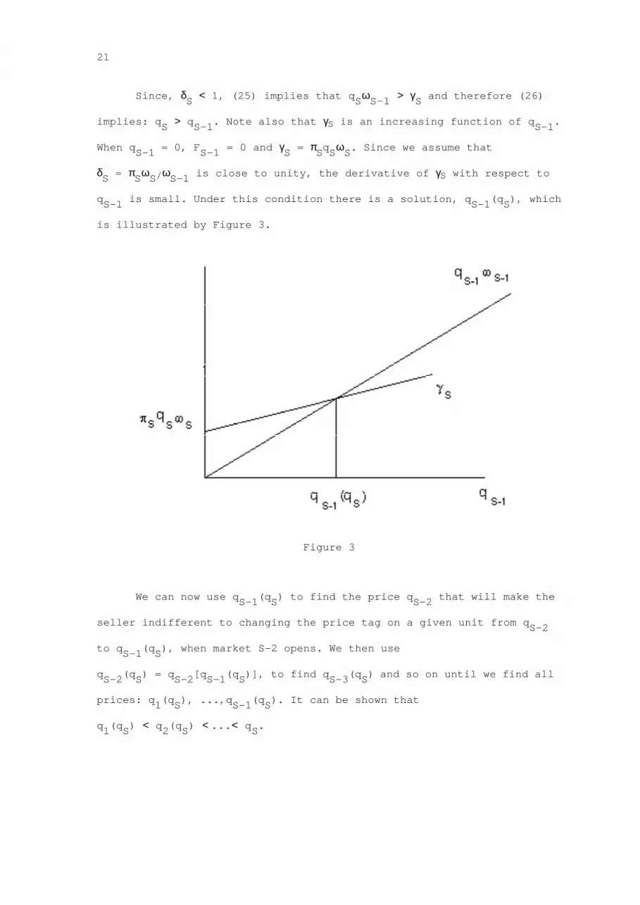
Since, δ S < 1, (25) implies that q Sω S-1 > γ S and therefore (26)

implies: q S > q S-1. Note also that γS is an increasing function of q

S-1.

When q S-1 = 0, F

S-1 = 0 and γ S = π Sq

Sω S. Since we assume that

δ S = π Sω S/ω S-1 is close to unity, the derivative of γS with respect to

q S-1 is small. Under this condition there is a solution, q

S-1(q

S), which

is illustrated by Figure 3.

Figure 3

We can now use q S-1(q

S) to find the price q

S-2 that will make the

seller indifferent to changing the price tag on a given unit from q S-2

to q S-1(q

S), when market S-2 opens. We then use

q S-2(q

S) = q

S-2[q

S-1(q

S)], to find q

S-3(q

S) and so on until we find all

prices: q 1(q

S), ...,q

S-1(q

S). It can be shown that

q 1(q

S) < q 2(q

S) < ...< q S.

22

We now use (19) to compute the total amount required to satisfy

the demand in market s:

(27) k s(q

S) = Σsj=1 ∆ jF

j[p

j(q

S), q

s(q

S)]/q

s(q

S).

Since q 1(q

S) < q 2(q

S) < ...< q S, total demand,

d(q S) = ΣSs=1k

s(q

S), is large when q

S is small. Since

q s(q

S) > δ s+1q

s+1(q

S), total demand d(q

S) is small when q

S is large.

Supply is given by (22) which can be written as:

(28) v'(k) = βΓ 1(q S)z(q

S) = βq 1(q

S)ω 1z(q

S),

where z(q S) = ΣSi=1 F

1[ΣSj=1 q

j(q

S)/S, q

i(q

S)]/q

i(q

S). Since v'(0) = 0 and

v'( ) is increasing, there exists a solution, s(q S) = k(q

S), to (28).

We now equate supply and demand:

(29) s(q S) = d(q

S).

We denote the solution to (29) by q̂ S and compute all equilibrium prices

and quantities: q s(q̂

S), k

s(q̂

S).

Note that the real wage term (the right hand side of [28]) is:

βω 1ΣSi=1 [q 1(q

S)/q

i(q

S)]F

1[ΣSj=1 q

j(q

S)/S, q

i(q

S)]. Therefore, if the

elasticity of q i with respect to qS is unity, the real wage will not be

affected by the change in q S. The intuition is that when all prices

change by the same proportion, the change in the purchasing power

completely offset the change in current prices. It is therefore possible

that supply is flat as in Figure 4.

23

Figure 4

Discussion:

There is an ongoing debate about modeling prices. Some believe

that in the real world prices are sticky. Other believe that prices are

completely flexible. Here I propose a sequential trading model that may

bridge the gap between these two approaches. In the proposed UST model

sellers announce prices in advance but do not have an incentive to

change them during the trading process: Prices look as if they are

sticky but they are not.

Some researchers argue that in the real world sellers are eager to

sell and therefore we should assume demand satisfying behavior in our

24

models. In a UST equilibrium sellers are eager to sell but not

necessarily at the cheapest price. Thus the UST framework allows for a

"new Keynsian" interpretation which assumes sticky prices and some

demand satisfying commitment. It also allows for a competitive

interpretation that assumes flexible prices. Under both interpretations

there is a positive relationship between output (capacity utilization)

and money.

The UST model in this paper is more realistic than previous UST

models. In previous UST models buyers buy at the cheapest available

price so that cheaper goods are sold first (as in Prescott [1975]). Here

buyers may buy at prices which are higher than the cheapest alternative

and therefore in equilibrium the trade-off is between average capacity

utilization and the price. This added realism is important for the

analysis of micro data.

The UST model assumes a two stage production process and allows

for price dispersion. I argue against the alternative of a single-price

single-production-stage environment. These assumptions are not

realistic. Price dispersion is observed and sellers do not always

satisfy demand at the cheapest price. More importantly, the single-

price model does not yield a monotonic relationship between money and

output. This is because in a cash-in-advance model, money earned today

is spent in the next period and therefore when sellers observe a high

money injection they expect a high next period price level and a low

real wage. The real wage effect operates in the direction of a negative

relationship between money and output. This effect becomes even more

important when sale promotion is allowed.

25

What is the importance of the real wage effect in other sticky

price models? In a Taylor (1980) or a Calvo (1983) type model it is

possible that only a small fraction of the sellers change their nominal

prices each period. In this case a seller who observes a high money

supply will not adjust his expectations about the next period price

level by much. The real wage effect may therefore be unimportant if we

keep the assumption that sellers must satisfy demand. But if we relax

this assumption we may find that the real wage effect is important

because a high money supply is likely to have a negative effect on the

probability of making a buy in the next period (the ratio of nominal

supply to nominal demand). This will reduce the real wage because there

is now a higher probability that money earned today will be spent in the

more distant future (say 2 periods from now).

Thus, I question the micro-foundation of the new-Keynsian

economics. In particular, relaxing the assumption that demand must be

satisfied at the sticky-price makes a difference in the model we studied

and is likely to make a difference in other sticky-price models. The UST

alternative has a Keynsian flavour. Sellers are eager to sell and prices

look sticky. The policy implications however are neo-classical. Capacity

utilization and welfare will be maximized when money surprises are

eliminated (see Eden [1994] for example).

26

APPENDIX: ALLOWING FOR NON-PRICE COMPETITION IN THE STICKY-PRICE MODEL

Here I allow for non-price competition by using

w i = exp[α(p/p i) - γ(Y/Y i)], where Y

i is the amount of labor employed

by firm i, Y is the average per firm amount of labor and γ > 0 is a

parameter. I show that in a single-sticky-price equilibrium the

output/money relationship may be negative under this specification.

I start by computing the revenue function in a way which is

similar to the derivation of (4). When x ≤ ζ and all other sellers quote

the price p and produce the output Y, a seller who quotes the price p i

and produces the amount Y i will get:

(A1) r(p i, Y

i, p, Y, x) = (1 + x)exp[α(p/p i) - γ(Y/Y i)]/exp(α - γ),

normalized dollars if he satisfies demand and p iY i otherwise. When

x > ζ, the seller can sell as much as he wants at the price p i.

The household takes p, ζ and the functions Π(x) and

r(p i, Y

i, p, Y, x) as given and solves (7) after replacing the revenue

function R(p i, p, x) with r(p

i, Y

i, p, Y, x). When x ≤ ζ and other

sellers satisfy demand the labor supply choice is (5). The first order

condition for this problem are given by (11) and:

(A2) v'(L) = βV'r 2/(1 + x), if r(p

i, L, p, Y, x) < p iL ;

(A3) v'(L) = βV'p i/(1 + x), if r(p i, L, p, Y, x) > p iL ;

(A4) βV'r 2/(1 + x) ≤ v'(L) ≤ βV'p i/(1 + x),

27

if r(p i, L, p, Y, x) = p iL ;

where r 2 = ∂r/∂L = (γ/L)r(p i, L, p, Y, x) = γr/L is the return to sale

promotion. Note that the return to sale promotion is proportional to

average revenues r/L.

Conditions (A2) and (A3) say that the marginal cost must equal the

real wage. The first order condition (A2) must hold when there is excess

capacity. In this case an increase in labor by one unit will increase

revenues by r 2 = γr/L current normalized dollars which will become

r 2/(1 + x) normalized dollars in the next period. Therefore the real

wage for this case is: βV'r 2/(1 + x).

Condition (A3) must hold when there is excess demand. In this

case, the real wage is: βV'p i/(1 + x).

Condition (A4) must hold when the seller satisfies demand. In this

case, if the seller increases output by one unit he will get γr/L from

his promotion efforts. If he cuts labor by one unit he will lose p i

dollars. When γr/L < p i, the marginal cost must be between the real

wage βV'r 2/(1 + x) and the real wage βV'p i/(1 + x) because at the

optimum the seller cannot benefit from either increasing output or

reducing it.

When x > ζ, there is excess demand and the seller can sell as much

as he wants at the price p i. The first order condition in this case is

(10).

Equilibrium is a pair (p, ζ) and a vector of functions

[Π(x), Y(x), L(x), r(p i, Y i, p, Y, x)] such that (A1) is satisfied and:

28

(a) Given (p, ζ) and the functions {Π(x), r[p i, Y i, p, Y(x), x]}, the

price p i = p and the output L(x) = Y(x) solve (7) after replacing R( )

by r( );

(b) Π(x) = min{1, pL(x)/(1 + x)};

(c) 1 + x ≤ pL(x) for all x ≤ ζ and 1 + x > pL(x) for x > ζ.

In equilibrium, r(p, L, p, Y, x) = 1 + x. The first order

conditions (A2) and (A4) must hold when x ≤ ζ and

1 + x ≤ pL(x). The first order condition (10) must hold when x > ζ and

1 + x > pL(x). These conditions can be written in equilibrium as:

(A5) v'(L) = γA/pL, if 1 + x < pL(x);

(A6) γA/(1 + x) ≤ v'(L) ≤ Α/(1 + x)

if 1 + x = pL(x);

(A7) v'(L) = A/(1 + x), if 1 + x > pL(x); .

where A = βπ/(1 - β + πβ).

There is a unique solution, L*, to (A5). Thus, when there is

excess supply the equilibrium labor supply does not depend on x. The

intuition is as follows. When 1 + x < pL, the benefit from increasing

labor is in promotion of sales. In equilibrium an additional unit of

labor will increase revenues by (γ/L)(1 + x) current period normalized

dollars and by (γ/L) next period's normalized dollars. Since next

period's normalized dollars is the relevant measure, the promotion

29

benefit does not depend on x and therefore when the marginal benefit is

due to sale promotion, labor supply does not depend on x.

We now distinguish between two cases: γ > 1 and γ ≤ 1. When γ ≤ 1,

the marginal cost as a function of x is given by the solid line in

Figure A1. When x ≤ pL* - 1, there is excess capacity and the marginal

benefit (due to sale promotion) is constant and is equal to the marginal

cost: γA/pL*. Capacity is fully utilized when x = pL* - 1. When

pL* - 1 ≤ x ≤ ζ, the seller satisfy demand and the marginal cost is

given by v'[(1 + x)/p]. In this region the marginal benefit from selling

an additional unit at the price p (= A/1+x) is greater than the marginal

cost but the seller does not increase output because he is constraint by

demand. When x > ζ, there is excess demand and the seller can sell as

much as he wants at the quoted price p. He therefore chooses marginal

cost equal to the marginal revenues in this range.

Figure A1

30

Since labor is a monotonic function of the marginal cost, it has

three regions as in Figure A2.

Figure A2

We now turn to the case γ > 1. In this case, condition (A6) is

never satisfied. At x = ζ, the marginal cost drops from the constant

promotion level (γA/pL*) to the unconstraint level (A/1+x). This is

illustrated by Figure A3. The implied equilibrium labor supply function

is in Figure A4.

31

Figure A3

Figure A4

We may summarize the discussion as follows.

32

Claim 2: When sale promotion is allowed labor supply is not a strictly

increasing function of x even in the excess supply range (x ≤ ζ). When

γ > 1, the equilibrium labor supply function is weakly decreasing in x

in the entire range. When γ ≤ 1, the equilibrium labor supply is not a

monotonic function of x: It is flat at first, then increasing and then

decreasing.

REFERENCES

Akerlof, George and Yellen, Janet "Can Small Deviations from Rationality

Make Significant Differences to Economic Equilibria?" The

American Economic Review, Sep. 1985, Vol. 75, pp. 708-21.

Barro Robert J. and Herschel I. Grossman., "A General Disequilibrium

Model of Income and Employment" The American Economic Review,

Vol. 61, No. 1. (Mar., 1971), pp. 82-93.

Bental, Benjamin and Benjamin Eden., "Money and Inventories in an

Economy with Uncertain and Sequential Trade", Journal of

Monetary Economics, 37 (1996) 445-459.

Blanchard Olivier Jean., and Kiyotaki Nobuhiro "Monopolistic Competition

and the Effects of Aggregate Demand" The American Economic

Review, Sep. 1987, Vol. 77, No.4, pp. 647-666.

Calvo, Guillermo A., "Staggered Prices in a Utility-Maximizing

Framework" Journal of Monetary Economics, XII (1983),383-398.

Dixit Avinash, "Quality and Quantity Competition" The Review of Economic

Studies, Vol. 46, Issue 4 (October 1979), 587-599.

Dixit, Avinash and Stiglitz, Joseph "Monopolistic Competition and

Optimum Product Diversity" The American Economic Review, June

1977, Vol. 67, pp. 297-308.

Eden, Benjamin. "The Adjustment of Prices to Monetary Shocks When Trade

is Uncertain and Sequential" Journal of Political Economy, Vol.

102, No.3, 493-509, June 1994.

33

Lucas, Robert. E., Jr. and Michael Woodford "Real Effects of Monetary

Shocks In an Economy With Sequential Purchases" Preliminary

draft, The University of Chicago, April 1994.

Manski, Charles F. "Daniel McFadden and the econometric analysis of

discrete choice" November 2000. Taken from Charles Manski's web

page, Department of Economics, Northwestern University.

McFadden Daniel "Disaggregate Behavioral Travel Demand's RUM Side: A 30-

Year Retrospective" mimeo, March 2000 (taken from McFadden's web

page, http://emlab.berkeley.edu/users/mcfadden/).

__________ "Conditional Logit Analysis of Quantitative Choice Behavior,"

in P.Zarembka (ed.), Frontiers in Econometrics, 105-142,

Academic Press: New York, 1973.

__________ "Quantitative Methods for Analyzing Travel Behavior of

Individuals: Some Recent Developments" in D.Hensher and

P.Stopher (eds.), Behavioral Travel Modelling, 279-318, Croom

Helm London: London, 1978.

Prescott, Edward. C., "Efficiency of the Natural Rate" Journal of

Political Economy, 83 (Dec. 1975): 1229-1236.

Spence Michael, "Nonprice Competition" The American Economic Review,

Vol. 67, Issue 1, Papers and proceedings, Feb. 1977, 255-259.

Stigler, George. "Price and Non-Price Competition" Journal of Political

Economy, Vol.76, Issue 1 (Jan.-Feb. 1968), 149-154.

Taylor, John B., "Aggregate Dynamics and Staggered Contracts" The

Journal of Political Economy, Vol. 88, No. 1. (Feb.,1980), pp.

1-23.

Williamson, Stephen D. "Sequential Markets and the Suboptimality of the

Friedman rule" Journal of Monetary Economics; 37(3), June 1996.

Woodford, Michael "Loan Commitments and Optimal Monetary Policy" Journal

of Monetary Economics; 37(3), June 1996, 573-605.

34