Streamwise vortices and transition to turbulence

J. Fluid Mech. (1994), vol. 264, p p . 185-212 Copyright 0 1994 Cambridge University Press

185

Streamwise vortices and transition to turbulence

By JAMES M. HAMILTON? A N D FREDERICK H. ABERNATHY

Division of Applied Sciences, Harvard University, Cambridge, MA 02138, USA

(Received 19 September 1992)

A series of experiments was conducted to determine the conditions under which streamwise vortices can cause transition to turbulence in shear flows. A specially designed obstacle was used to produce a single vortex in a water-table flow, and the design of this obstacle is discussed. Laser-Doppler velocimetry measurements of the streamwise and crossflow velocity fields were made in transitional and non-transitional flows, and flow visualization was also used. It was found that strong vortices (vortices with large circulation) lead to turbulence while weaker vortices do not. Determination of a critical value of vortex strength for transition, however, was complicated by ambiguities in calculating the vortex circulation. The profiles of streamwise velocity were found to be inflexional for both transitional and non-transitional flows. Transition in single-vortex and multi-vortex flows was compared, and no qualitative differences were observed, suggesting no significant vortex interactions affecting transition.

1. Introduction One of the goals of transition research is to develop methods for the prediction and

control of laminar-to-turbulent transition. Such methods should apply to internal and external flows, two- and three-dimensional flows, transition due to finite-amplitude and infinitesimal disturbances from any source, and transition due to surface irregularities and pressure gradients. At present, however, transition theory is principally concerned with the primary and secondary instabilities of two-dimensional laminar base flows. And while these efforts have produced a fascinating collection of instability mechanisms, there is not, as yet, any prediction scheme which incorporates these mechanisms.

Among those prediction procedures which have been proposed, the most often cited, the eN method, is used for prediction of transition in boundary layers. The eN method uses linear stability theory to determine the location at which the most unstable two- dimensional disturbances will have grown by some factor. The critical value of this amplification factor, where transition occurs, must be determined empirically. This approach would be useful if the transitional amplification factor were constant for all laminar boundary layers and test conditions, yet this does not appear to be the case. For example, Horstmann, Quast & Redeker (1990) found, for both wind-tunnel and flight tests of an airfoil, that an amplification factor of about e13.5 corresponded to the observed location of transition. The values obtained by Obara & Holmes (1985) in flight tests of a different airfoil were significantly larger: el5 to el’. In addition, Obara & Holmes concluded that transition in their experiments occurred owing to a laminar

t Present address: 3715 Linwood Avenue, Oakland, CA 94602, USA.

186 J. M . Hamilton and F. H. Abernathy

separation bubble on the airfoil. Had no such bubble been present, the amplification factor at transition would have been even higher. The obvious flaw of the eN method is its oversimplification of the transition process. It has long been known (e.g. Klebanoff, Tidstrom & Sargent 1962) that boundary-layer transition involves three- dimensional, finite-amplitude (nonlinear) disturbances. The eN approach completely ignores these effects. Moreover, in some flows, the use of an amplification factor is completely inappropriate, as in the case of the laminar separation bubble on an airfoil, or in a linearly stable flow such as in a pipe, for which the eN method would incorrectly predict that transition would never occur.

The ideal prediction scheme would provide not only broad application and freedom from the requirement of empirical calibration, but would also offer insight into methods of transition control. Any (hypothetical) scheme which incorporated all the known features of transition would be so complicated as to provide little useful insight. Instead, transition must be reduced to some critical process, common to all transitional flows, without which turbulence would not develop. One hint of the existence of such a critical process is the observation that transition is virtually always preceded by the appearance of streamwise vortices. Though these vortices are produced by any of a number of processes, the final disintegration of the vortex into turbulence may be due to a single mechanism. If this is the case, prediction of transition would be a matter of determining whether vortices of the proper characteristics were present in any given flow. Transition control would involve modification of streamwise vortices to cause or prevent transition, as desired.

Given the nearly universal presence of streamwise vortices in transitional flows, it is somewhat surprising that the process by which these vortices break down into turbulence has not been extensively studied. To some degree, the tendency of researchers to focus on other aspects of transition is due to a widespread belief that the breakdown mechanism is already known: the instability of the mean flow due to shear layers, or inflexions in the streamwise velocity profiles, produced by the vortices. Inflexional velocity profiles are known to be important in two-dimensional stability theory, and such profiles have indeed been observed in transition experiments. However, most of these experiments have involved flows in which transition to turbulence was inevitable, thus no comparison of transitional and non-transitional flow characteristics was possible. Consequently, many researchers have reached the implicit conclusion that inflexional velocity profiles always lead to turbulence, while others refer, instead, to ‘sharply’ or ‘steeply’ inflexional velocity profiles as the cause of breakdown. It is certainly not the case, however, that all inflexional profiles lead to turbulence, nor that breakdown requires particularly ‘ sharp ’ inflexions in the velocity profiles, as the results of the present investigation will make clear. Before proceeding with these results, however, it is useful to briefly review inflexional velocity profiles and stability theory, as well as the observations of previous investigators.

The creation of inflexions in the profiles of streamwise velocity is part of the general redistribution of momentum effected by streamwise vortices. To one side of a vortex, low-momentum fluid is advected away from the wall region, displacing faster moving fluid and creating a region of relatively low speed. On the other side of the vortex, high- momentum fluid is pushed toward the wall, producing a high-speed region. This redistribution of momentum is often described in conjunction with counter-rotating vortex pairs, but it is clear that only a single vortex is required. The wall-normal profiles of streamwise velocity in the high-speed region are more full than the average profile, while those in the low-speed region tend to be inflexional, corresponding to a three-dimensional shear-layer detached from the wall.

Streamwise vortices and transition to turbulence 187

Two-dimensional flows with this type of inflexional velocity profile satisfy the necessary conditions for instability (Rayleigh’s inflexion-point theorem and Fjerrtoft’s theorem, see e.g. Drazin & Reid 198l), and it is by analogy with two-dimensional theory that the breakdown of vortices into turbulence is often considered to be due to an inflexional instability. The classic example of an inflexional instability is the Helmholtz vortex sheet instability (Craik 1985). The inviscid base flow is two- dimensional and unbounded, and the vortex sheet is due to a velocity discontinuity. There is no inherent lengthscale in this problem, and the flow is unstable to infinitesimal disturbances of all wavelengths. In any real (viscous) flow, a lengthscale would be introduced by the finite thickness of the vortex sheet, or shear layer, and a bounded flow would possess an additional lengthscale. Such flows are easily modelled (e.g. Drazin & Reid 1981) and the results are well known: the finite thickness of the shear layer imposes a short-wavelength cutoff on the instability, and the presence of boundaries prevents the growth of disturbances with wavelengths greater than some value. When long- and short-wavelength stability regions overlap, the flow is stable to all disturbances. Thus, while an inflexional velocity pressure is a necessary condition for the instability of an inviscid, two-dimensional shear flow, it is not sufficient.

Since there is no general theory for the stability of three-dimensional flows, one must turn to experiments (either laboratory or numerical) to examine the role of streamwise vortices and inflexions in transitional flows. The most influential early study is due to Klebanoff et al. (1962). The vibrating ribbon technique was used to produce artificial disturbance waves in the boundary layer of a flat plate. As the flow evolved downstream of the ribbon, the disturbance waves developed a complicated three- dimensional structure, including ‘ longitudinal ’, or streamwise, vortices. Still further downstream, the flow underwent an ‘abrupt change in the character of the wave motion’, with the appearance of high-frequency (relative to the fundamental ribbon frequency) fluctuations of the streamwise velocity. This abrupt change was termed ‘breakdown’, and preceded the appearance of fully turbulent flow. A more recent study is due to Swearingen & Blackwelder (1987). In their experiments the centrifugal, or Gortler, instability of a flow along a concave wall was used to generate streamwise vortices. Redistribution of momentum by the vortices resulted in low- and high-speed regions and the associated inflexions in both the wall-normal and spanwise profiles of streamwise velocity. Flow breakdown was identified in several ways, including smoke-wire flow visualization and measurements of the intensity (r.m.s.) of temporal fluctuations of the streamwise velocity. The flow fields in both sets of experiments contained inflexional velocity profiles. However, neither the experiments of Klebanoff et al., nor of Swearingen & Blackwelder included any non-transitional flows; only flows which eventually became turbulent were considered. Thus, it is difficult to determine from these experiments whether inflexional velocity profiles inevitably lead to vortex breakdown and turbulent flow, or whether, as in the two-dimensional case, other parameters govern the process.

Other investigations have provided comparisons between non-transitional and transitional flows, and the experiments of Yang (1987) and Suri (1988) clearly show that inflexional velocity profiles do not necessarily produce turbulent flow. In Yang’s experiments a specially designed obstacle, placed into a water-table flow (see $2.1), was used to produce a pair of streamwise vortices spaced sufficiently far apart to prevent interaction. Yang found that while a single streamwise vortex always induced inflexions in the streamwise velocity profiles, transition occurred only when the strength, or circulation, of the vortex was above some critical value. This result helps to explain why Klebanoff et al. and Swearingen & Blackwelder always observed vortex


breakdown. In the case of Klebanoff et al. the experiments were conducted in a flow regime in which the two-dimensional waves continued to grow downstream of the vibrating ribbon. As a result, streamwise vortices produced by these waves grew in strength until breakdown occurred, regardless of the initial ribbon amplitude. In the same way, the curved wall in the experiments of Swearingen & Blackwelder caused continuous strengthening of the Gortler vortices with distance downstream until, ultimately, breakdown occurred.

Yang’s results are important not only because they challenge the assumption that any inflexion will lead directly to vortex breakdown, but also because they provide a possible basis for methods of transition prediction and control. If, indeed, the vortex strength is the sole parameter controlling transition, then accurate prediction of transition requires only a determination of the strength of vortices anticipated in a particular flow. Any number of methods can be used to make this determination, including, for example, relatively low resolution numerical simulations or empirical correlations of, say, wall roughness to vortex strength.

Unfortunately, equipment limitations prevented Yang from making direct measurements of the strength of the streamwise vortices in his experiments. Instead, measurements of the streamwise velocity field were used to deduce the vortex strength using the single vortex theory of Pearson & Abernathy (1984). Measurements in non- transitional flow suggested that the deduced vortex strength was also proportional to the depth times the velocity gradient at the wall of the unperturbed flow, and it was actually this quantity which was used in the transition experiments to infer that transition occurred above some critical value of the vortex strength.

Because of the importance of the conclusion that transition depends only on the strength of streamwise vortices in the flow, it was decided that verification by direct measurement of vortex strength in Yang’s single vortex flow would be worthwhile. At the same time, additional questions raised by Yang’s experiments could be addressed. For example, at vortex strengths approaching the critical value, evidence of a second, weaker vortex appeared. This raises the question of whether transition was not actually caused by some interaction between the two vortices. Also, Yang did not address the inflexional instability hypothesis in any detail beyond the observation that inflexions could occur without causing transition : his primary focus was on the vortex strength. Thus, he did not examine the flow for, say, rapid steepening of shear layers just before transition.

One question raised by Yang’s work and subsequently addressed by Suri (1988) concerns the universality of his conclusions: the vortex strength may be important in the single vortex flow, but what about more complicated flows? Suri used the vibrating ribbon technique to produce a complex array of streamwise vortices, also in a water- table flow. The flow regime was such that two-dimensional waves from the ribbon were always damped; thus, the maximum vortex strength achievable depended upon the original wave amplitude. Suri generally confirmed Yang’s conclusions, with only a slight modification. He found that when the strength of streamwise vortices is rapidly changing, it is not only the strength of the vortex that is important, but also the time available for the vortex to affect the flow. Unfortunately, however, Suri too was unable to make direct measurements of the crossflow, and he had to deduce the vortex strength from measurements of the streamwise velocity.

The present paper reports the results of direct measurements of the crossflow and streamwise velocities in the single-vortex flow. Two cases are examined in detail and are referred to here as the transitional flow and the non-transitional flow. In the non- transitional flow, the vortex simply decays downstream of the vortex generator, and the


flow remains laminar. In the transitional flow, the flow becomes turbulent downstream of the generator. In addition, a comparison is made of transition in the single-vortex flow and in a multiple-vortex flow. The term ‘transition’ rather than ‘breakdown’ is used throughout the remainder of this paper, since breakdown has come to denote, in the literature, an instability process with specific characteristics. The stability of the flow is not directly at issue here, as the growth or decay of small disturbances is not measured. The question, instead, is whether or not the flow becomes turbulent, and thus the term transition is more appropriate. The coordinate directions x, y and z denote the streamwise, wall-normal and spanwise directions, and the associated velocities are denoted u, v and w. Components of vorticity are given a subscript, e.g. w,. Dimensional quantities, e.g. U, are upper case, with the exception of kinematic viscosity, which is given the usual symbol v.

2. Experimental apparatus 2.1, Water-table $ow facility

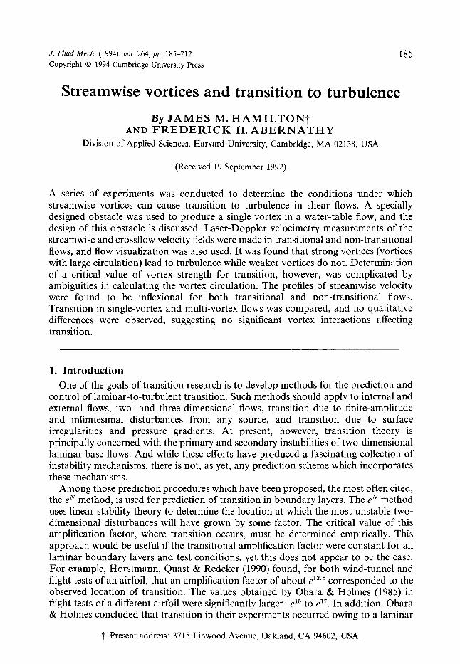
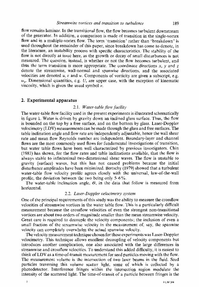
The water-table flow facility used in the present experiments is illustrated schematically in figure 1. Water is driven by gravity down an inclined glass surface. Thus, the flow is bounded on the top by a free surface, and on the bottom by glass. Laser-Doppler velocimetry (LDV) measurements can be made through the glass and free surfaces. The table inclination angle and flow rate are independently adjustable, hence the wall shear rate and mean flow Reynolds number are independent. Boundary-layer and channel flows are the most commonly used flows for fundamental investigations of transition, but water table flows have been well characterized by previous investigators. Chin (1981) has shown, for the flow rates and table inclinations available, that the flow is always stable to infinitesimal two-dimensional shear waves. The flow is unstable to gravity (surface) waves, but this has not caused problems because the initial disturbance amplitudes have been minimized. Bertschy (1979) showed that a turbulent water-table flow velocity profile agrees closely with the universal, law-of-the-wall profile, the deviation between the two being only 5-6 %.

The water-table inclination angle, 0, in the data that follow is measured from horizontal.

2.2. Laser-Doppler velocimetry system One of the principal requirements of this study was the ability to measure the crossflow velocities of streamwise vortices in the water table flow. This is a particularly difficult measurement because the crossflow velocities of even the strongest non-transitional vortices are about two orders of magnitude smaller than the mean streamwise velocity. Great care is required to decouple the velocity components; the inclusion of even a small fraction of the streamwise velocity in the measurement of, say, the spanwise velocity can completely overwhelm the actual spanwise velocity.

The velocity measurement technique chosen for these experiments was Laser-Doppler velocimetry. This technique allows excellent decoupling of velocity components but introduces another complication, one also associated with the large differences in streamwise and crossflow velocities. To understand this added difficulty, it is easiest to think of LDV as a time-of-transit measurement for seed particles moving with the flow. The measurement volume is the intersection of two laser beams in the fluid. Seed particles traversing this volume scatter light, some of which is collected by a photodetector. Interference fringes within the intersectioa region modulate the intensity of the scattered light. The time-of-transit of a particle between fringes is the

7 F L M 264

190 J. M. Hamilton and F. H. Abernathy

Foam wave damper

Flow straighteners

Overflo Pipe

Table angle adjustment

w-rate control valve

FIGURE 1. Water-table flow system.

period of the modulated intensity signal. When the fringes are oriented parallel to the flow, the time-of-transit is infinite, since particles never pass from one fringe to the next, and the measured velocity is zero. Unfortunately, when the velocity component parallel to the fringes is much greater than the normal component, the measured velocity is also zero, because the particle is unable to pass between fringes in the short time the particle resides in the measuring volume, i.e. the particle passes through the volume before crossing any fringes. To overcome this, ‘frequency shifting’ is used. The frequency of one of the beams is ‘shifted’, resulting in apparent motion of the fringes across the measuring volume. Thus, even particles moving exactly parallel to the instantaneous fringes have a measured velocity component normal to the fringes. In a sense, the fringes are now moving past the particle, rather than the particle moving between fringes. The actual velocity component normal to the fringes is simply the measured velocity minus the fringe velocity. In the water-table flow, as the streamwise velocity increases relative to the spanwise velocity, the required fringe velocity increases, and the actual spanwise velocity becomes the difference of two large numbers. If measurements could be made with infinite precision and accuracy, frequency shifted LDV measurements would be correct regardless of the relative magnitudes of the velocity components. In practice, however, measurements are uncertain and the use of frequency shifting can magnify this uncertainty. As an example, a flow in which the spanwise component of velocity is 1 YO of the streamwise component might require a fringe velocity equal to the streamwise velocity. If the velocity (particle velocity plus fringe velocity) can be measured to within 1 %, the uncertainty of the particle velocity measurement is 100 YO. Uncertainty is minimized by the use of the smallest shift feasible for the flow conditions. Also, the uncertainty tends to be lowest near the wall, where the streamwise velocity is lowest.

The LDV system used for the experiments presented here was designed and built specifically for measurement of streamwise vortices in the water-table flow. The system measured only one velocity component at a time, but the optics module could be rotated to measure either the streamwise or spanwise velocity component. Rotation of the optics module rotated the fringes in the measuring volume parallel to or perpendicular to the stream direction. Frequency shifting was used for spanwise


(4 Flow direction

1 2.5 mm r,

Water

Vortex generator

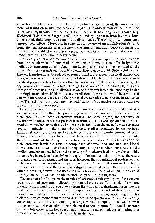
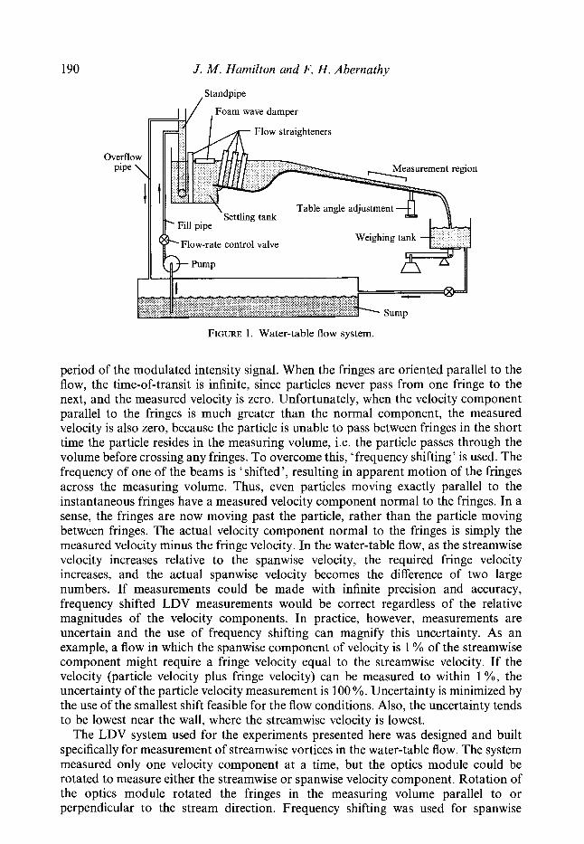
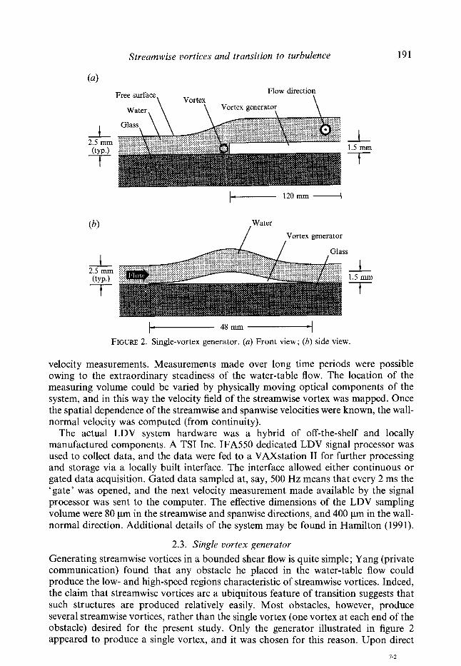
k- 48 mm -4 FIGURE 2. Single-vortex generator. (a) Front view; (b) side view.

velocity measurements. Measurements made over long time periods were possible owing to the extraordinary steadiness of the water-table flow. The location of the measuring volume could be varied by physically moving optical components of the system, and in this way the velocity field of the streamwise vortex was mapped. Once the spatial dependence of the streamwise and spanwise velocities were known, the wall- normal velocity was computed (from continuity).

The actual LDV system hardware was a hybrid of off-the-shelf and locally manufactured components. A TSI Inc. IFA550 dedicated LDV signal processor was used to collect data, and the data were fed to a VAXstation I1 for further processing and storage via a locally built interface. The interface allowed either continuous or gated data acquisition. Gated data sampled at, say, 500 Hz means that every 2 ms the ‘gate’ was opened, and the next velocity measurement made available by the signal processor was sent to the computer. The effective dimensions of the LDV sampling volume were 80 pm in the streamwise and spanwise directions, and 400 pm in the wall- normal direction. Additional details of the system may be found in Hamilton (1991).

2.3. Single vortex generator Generating streamwise vortices in a bounded shear flow is quite simple; Yang (private communication) found that any obstacle he placed in the water-table flow could produce the low- and high-speed regions characteristic of streamwise vortices. Indeed, the claim that streamwise vortices are a ubiquitous feature of transition suggests that such structures are produced relatively easily. Most obstacles, however, produce several streamwise vortices, rather than the single vortex (one vortex at each end of the obstacle) desired for the present study. Only the generator illustrated in figure 2 appeared to produce a single vortex, and it was chosen for this reason. Upon direct

1-2


measurement of the crossflow velocities, however, it has become clear that while this generator does produce a single vortex, the overall structure is more complicated than had been expected. Before presenting these results, though, it is useful to examine the mechanisms by which streamwise vortices are produced, and in particular how the single-vortex generator works.

The easiest way to describe the formation of streamwise vortices is to begin with the equation for the evolution of the streamwise component of vorticity, ox, for a general, incompressible flow

au au au 1 Dt ax az Re -- Dux - wx--+o -~uz-+-V2wx.

The Reynolds number, Re, is defined by some characteristic length and velocity. The first term on the right side of (1) represents streamwise (x) vorticity production due to stretching of vorticity-line elements, and the following two terms represent an increasing streamwise component of vorticity due to rotation of vorticity-line elements (e.g. Batchelor 1967). A two-dimensional shear flow, such as an idealized water-table flow, has only spanwise vorticity, o,. When this flow is perturbed, by a three- dimensional obstacle, say, au/i3z becomes non-zero, and streamwise vorticity can readily be produced from spanwise vorticity, as represented by the o, i3u/az term of (1). Physically, this corresponds to spanwise vorticity lines ‘wrapping’ around the obstacle, developing a streamwise orientation.

While a qualitative examination of the terms of (1) provides some insight into the production of streamwise vorticity, it is less clear when streamwise vortices form, or ‘roll-up’, from this vorticity. This question can only truly be answered by solving the equations of motion for the flow of interest. The rule of thumb, however, seems to be that concentrations of vorticity roll-up, while relatively homogeneous regions of vorticity do not. For example, when spanwise vorticity lines wrap around a hemisphere attached to the wall on the water table, the regions of streamwise vorticity are concentrated, and streamwise vortices form. Unfortunately, streamwise vortices produced by this wrapping process always seem to occur in groups of more than one vortex. Apparently, several vortices form in stagnation regions on the upstream or downstream sides of the obstacles. The Gaussian-like profile of the single vortex generator has no upstream or downstream stagnation regions ; spanwise vorticity is advected smoothly up and over the generator, and multiple vortices do not form. In this case, the primary mechanism for production of streamwise vorticity is not rotation of spanwise vorticity into the streamwise direction, as denoted by the o, au/az term of (1). Instead, streamwise vorticity is produced at the solid boundary. This process is related to the diffusive term in (I), (1/Re)V2ux.

The rate at which vorticity produced at a solid boundary diffuses into the fluid is determined by the normal gradient of vorticity at the boundary and the vorticity diffusivity, or kinematic viscosity. For a solid boundary at, say, a constant y-value the flux of streamwise vorticity, in non-dimensional term, can be shown to be (Lighthill 1963)

Thus, a spanwise pressure gradient at the wall, together with the no-slip boundary condition, creates a streamwise vorticity source at the wall. This is essentially the mechanism by which the single-vortex generator produces streamwise vorticity, though the analogy is complicated by the fact that the obstacle is not a y = const. surface.


A qualitative description of the formation of a single vortex on the water table, then, goes as follows. The portion of the flow which passes over the obstacle decelerates slightly, causing an increase in pressure relative to the fluid which passes to either side. The pressure gradient results in a spanwise flow, toward the lower pressure at the ends of the generator, and streamwise vorticity is produced in accordance with (2). This vorticity is created at the solid surface of the generator and diffuses into the fluid at a rate determined by viscosity. The end of the generator is cut off sharply (see figure 2), and spanwise flow over this edge ‘injects’ rotational fluid into the bulk of the flow creating a concentration of streamwise vorticity which rolls up to form a vortex. Thus, roll-up occurs on a timescale associated with crossflow advection rather than diffusion. This is important at very high-flow Reynolds numbers, since streamwise vorticity produced by the vortex generator will advect well downstream of the generator before diffusing appreciably into the fluid, and roll-up would not occur without the sharp end of the generator. At lower flow Reynolds numbers, streamwise vorticity quickly diffuses into the bulk of the fluid; a streamwise vortex still forms from flow over the sharp edge of the generator, but may be all but obscured by a background of diffuse vorticity.

Of course, the fact that the flow decelerates over the obstacle suggests that there is some contribution to streamwise vorticity production by the w, au/az term of (1). Vorticity produced in this way is opposite in sign to vorticity produced by the spanwise pressure gradient, and presumably reduces the circulation of the streamwise vortex somewhat. The claim that the flow decelerates over the obstacle may seem contrary to the usual expectation that flow accelerates past obstructions in incompressible flow. Deceleration is a peculiar property of the water-table flow because the upper boundary of the flow is a free surface. When the mean flow velocity exceeds the maximum (long wavelength) speed of surface waves, obstructions result in an increased height of the free surface, and a reduced flow velocity (e.g. Sabersky, Acosta & Hauptmann 1971). The ratio of average fluid velocity to the shallow-water wave speed is the Froude number, and all water-table experiments referred to here have supercritical (> 1) Froude number.

3. Experimental results 3.1. Water-table base $ow

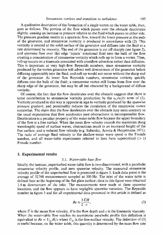
Ideally, the laminar, unperturbed water-table flow is two-dimensional, with a parabolic streamwise velocity profile, and zero spanwise velocity. The measured streamwise velocity profile of the unperturbed flow is presented in figure 3. Each data point is the average of 32768 measurements sampled at 500Hz. The inlet of the water table is defined here as the beginning of the flat glass surface; data in this figure were obtained 1.4 m downstream of the inlet. The measurements were made at three spanwise locations, and the flow appears to have negligible spanwise variation. The Reynolds number in figure 3 and for all experimental data presented in this article is defined as

3 UH Re = --,

2 v (3)

where U is the mean flow velocity, H is the flow depth and v is the kinematic viscosity. When the water-table flow reaches its asymptotic parabolic profile this definition is equivalent to Re = U,, H/v where U,, is the free-surface velocity. The definition of (3) is useful because, on the water table, this quantity is determined by the mass flow rate

I94 J. M . Hamilton and F. H. Abernathy

0.005

1 .o

0.8

0.6

Y 0.4

0.2

1 1 1 1 ~ 1 1 1 1 ~ 1 1 1 1 I I I I I I I I I I - - - - - -

- -

-

0 0.2 0.4 0.6 0.8 1.0

FIGURE 3. Water-table base flow. Streamwise velocity measurements at 3 spanwise locations relative to an arbitrary datum: A, z' = 0; 0, z' = 0.41 ; V, z' = 0.81 ; -, parabola fit to experimental data. Data obtained 1.4 m downstream of inlet. Re = 1900, 0 = 2.0", H = 2.45 mm, U , = 0.74 m s-l.

U

-0.005

-0.010

- - - - -v - - -

- - - -

I I I I I I I I I I I I I I I I I I I I I I

(at constant temperature), and is independent of the water-table angle. Also, it can be determined easily with the water-table weighing tank without direct velocity measurements. From figure 3, it appears that the flow has attained the asymptotic parabolic velocity profile, though, in fact, the flow is still developing as the flow depth


H continues to decrease slightly with distance downstream. Nevertheless, U,, is very nearly equal to $7, and the quantity

is used to normalize all streamwise velocities. The wall-normal distance in this figure is non-dimensionalized by the flow depth, H, as are all other lengths, and H i s always measured at a downstream location as close a possible to the vortex generator.

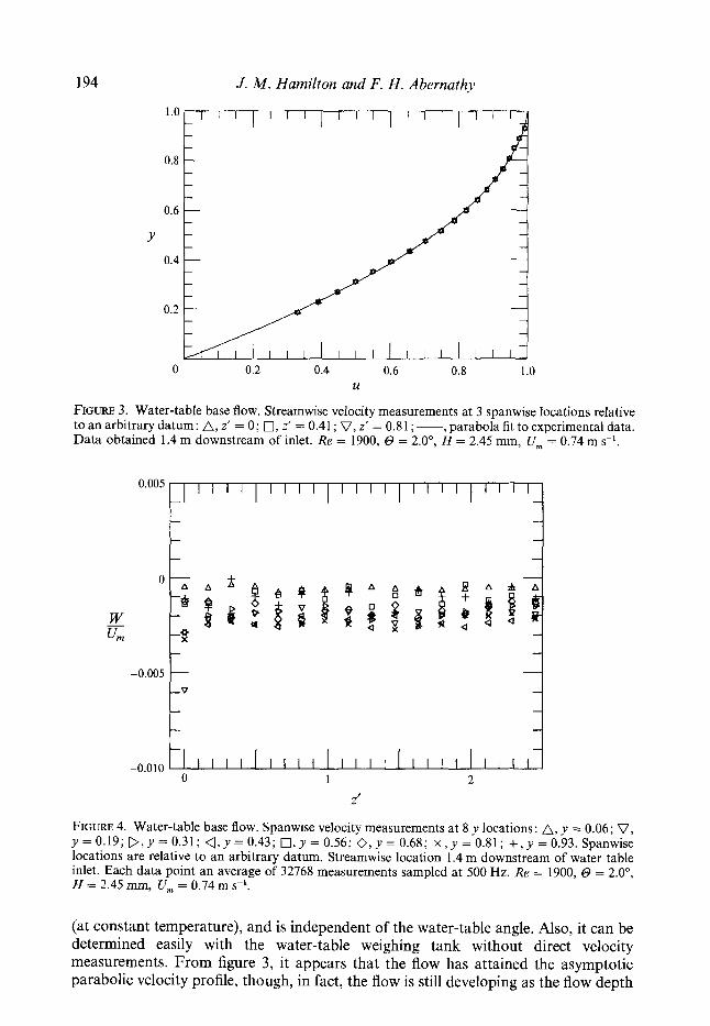
Measurements of the spanwise velocities of the unperturbed flow are presented in figure 4. These data show the spanwise velocity to be non-zero, but generally without spanwise dependence. The mean magnitude of the spanwise velocity is approximately 0.15 YO of the free-surface velocity Urn. This offset is due to a small misalignment of the LDV system such that part of the streamwise velocity is measured as spanwise velocity. As will be seen, the measured spanwise velocities of the single streamwise vortex are at least an order of magnitude larger than 0.15 % Urn, even well downstream of the generator where the vortex has decayed significantly.

3.2. Vortex crossflow measurements 3.2.1. Non-transitionalpow

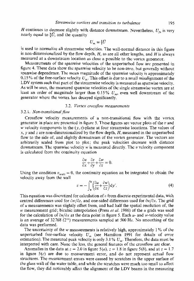
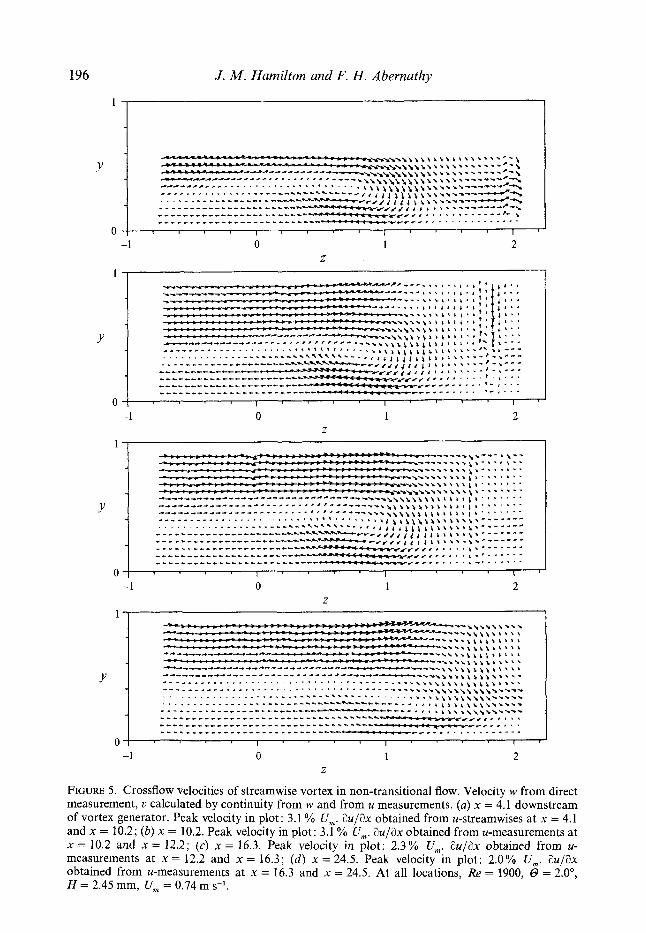
Crossflow velocity measurements of a non-transitional flow with the vortex generator in place are presented in figure 5. These figures are vector plots of the v and w velocity components in the (y, 2)-plane at four streamwise locations. The values of x, y and z are non-dimensionalized by the flow depth, H, measured in the unperturbed flow to the side of, and slightly downstream of the vortex generator. The vectors are arbitrarily scaled from plot to plot; the peak velocities decrease with distance downstream. The spanwise velocity w is measured directly. The z, velocity component is calculated from the continuity equation

au av a w ax ay a Z -+-+- = 0.

Using the condition vwazz = 0, the continuity equation an be integrated to obtain the velocity away from the wall

This equation was discretized for calculation of v from discrete experimental data, with centred differences used for aw/az, and one-sided differences used for &/ax. The grid of u measurements was slightly offset from, and had half the spatial resolution of, the w measurement grid; bicubic interpolation (Press et al. 1986) of the u grids was used for the calculation of au/ax at the data point in figure 5. Each u- and w-velocity value is an average of 32768 (215) measurements sampled at 500 Hz. No smoothing of the data was performed.

The uncertainty of the w measurements is relatively high, approximately 1 YO of the unperturbed free-surface velocity U, (see Hamilton 1991 for details of error estimation). The measured peak velocity is only 3.1 % U,. Therefore, the data must be interpreted with care. None the less, the general features of the crossflow are clear.

Anomalies in the data at z = 2.0 in figure 5(a), z = 1.8 in figure 5(b), and at z = 1.7 in figure 5(c) are due to measurement error, and do not represent actual flow structures. The measurement errors were caused by scratches in the upper surface of the glass wall of the water table, and while the scratches were much too small to affect the flow, they did noticeably affect the alignment of the LDV beams in the measuring

196 J. M. Hamilton and F. H. Abernathy

1

Y

0 -1 0 1 2

y L 0 -1 0 1 2

1

Y

0 -1 0 1

Z

2

FIGURE 5. Crossflow velocities of streamwise vortex in non-transitional flow. Velocity w from direct measurement, v calculated by continuity from w and from u measurements. (a) x = 4.1 downstream of vortex generator. Peak velocity in plot: 3.1 % Urn. &/ax obtained from u-streamwises at x = 4.1 and x = 10.2; (6) x = 10.2. Peak velocity in plot: 3.1 % Urn. &/ax obtained from u-measurements at x = 10.2 and x = 12.2; (c) x = 16.3. Peak velocity in plot: 2.3% Urn. au/ax obtained from u- measurements at x = 12.2 and x = 16.3; ( d ) x = 24.5. Peak velocity in plot: 2.0% Urn. a u p x obtained from u-measurements at x = 16.3 and x = 24.5. At all locations, Re = 1900, 0 = 2.0°, H = 2.45 mm, Urn = 0.74 m s-l.


volume. Scratches in the glass were sufficiently numerous that they could not be avoided entirely, but care was taken to obtain data only where scratches would not cause measurement errors in the core region of the vortex. This, in fact, was the primary basis for the selection of the streamwise location of the measurements in figure 5. The data set at x = 4.1 (figure 5a) is incomplete because of a slight depression of the free surface immediately downstream of the vortex generator.

The trailing edge of the vortex generator is located at x = 0, and positive x is downstream. The generator is located at z < 0, with the end of the generator at z = 0. The generator was not aligned squarely with the flow. Instead, it was rotated slightly in the positive direction about the y-axis. The origin of the coordinate system is the downstream right-hand corner of the generator, as viewed looking downstream. This point is located 1.36 m downstream of the water-table inlet. The data show that fluid which passed over the vortex generator has developed a spanwise velocity component, while the fluid which passed to the side of the generator has negligible spanwise velocity. The streamwise vortex has rolled-up between these regions. This is the mechanism described in $2. The top of the generator is at y = 0.61. Note that the vortex completely fills the region between the top of the generator and the wall, much like the recirculation region formed by flow over a backward-facing step.

Perhaps the most notable feature of these data is that the structure of the streamwise vortex remains relatively constant in the downstream direction. Even the width and height of the vortex are unchanged, and the distance from the vortex centre to the wall varies by no more than one grid length between streamwise stations. Only the magnitudes of the crossflow velocities change, as the streamwise vortex decays downstream of the generator, though the decay is not apparent in the plots because the vector lengths have been rescaled in each plot for visual clarity of the vortex structure.

The downstream decay of the crossflow, dropping from a peak cross-stream velocity of 3.1 YO Urn at x = 4.1 (figure 5a) to 2.0 Yo U, at x = 24.5 (figure 5 d ) occurs over a distance of over 20 flow depths. Spanwise variations of this magnitude occur over a much shorter lengthscale, on the order of one flow depth. Given this slow streamwise variation of the flow, a useful simplification might be to treat the velocity field as quasi- two-dimensional, that is, to assume a/& of any quantity is zero.

To test the plausibility of such an assumption, v velocities were calculated from experimental w measurements using continuity, equation (4), with the au/ax term set to zero. The results, when plotted, are virtually indistinguishable from figures 5 (and thus not replotted here), suggesting that the vortex structure is indeed well approximated with this quasi-two-dimensional assumption.

The circulation r of the vortex is defined by

with integration in the plane normal to the mean flow. The non-dimensional form of the circulation (following Pearson & Abernathy 1984 and Yang 1987) is the vortex Reynolds number Re,, defined as

r Re =L. (6)

- 2nv

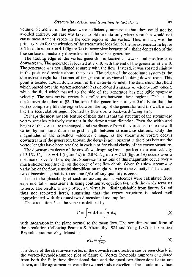
The decay of the streamwise vortex in the downstream direction can be seen clearly in the vortex-Reynolds-number plot of figure 6. Vortex Reynolds numbers calculated from both the fully three-dimensional data and the quasi-two-dimensional data are shown, and the agreement between the two methods is excellent. The circulation values

J, M . Hamilton and F. H. Abernathy

0 10 20 X

30

FIGURE 6. Vortex Reynolds number at various streamwise locations. 0, vortex Reynolds number calculated from full three-dimensional data of figure 5; a, vortex Reynolds number calculated from quasi-two-dimensional crossflow velocity data. Re = 1900, 0 = 2.0”, H = 2.45 mm. Circulation integration contour shown in figure 7.

1

FIGURE 7. Contour used for calculation of vortex Reynolds numbers in figure 6. The data in the plot are from figure 5(a).

are based on the integration contour of figure 7 (with illustrative data from figure 5a). This particular contour is of no special significance, and was chosen simply because it could be used consistently for comparison of data at all four streamwise locations for which data were obtained, even at x = 4.1. The issue of circulation contour selection is discussed in 93.4.

3.2.2. Transitional $ow Cross-flow measurements were also made in a transitional flow. The same vortex

generator was used as in the non-transitional flow; the water-table angle, 0, and the mean flow Reynolds number, Re, were increased to produce transition. Measurements were made at two streamwise locations. Transition was intermittent, with turbulent spots appearing downstream of the vortex generator every few seconds. Measurements at each data point were averaged over more than one minute (32768 samples at


1

0 -1 0 I 2

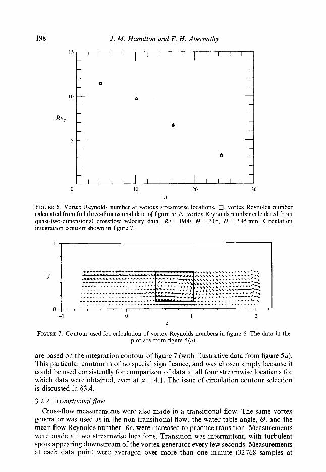
FIGURE 8. Crossflow velocities of streamwise vortex in transitional flow. Velocity w from direct measurement, u calculated by continuity from w assuming au/ax = 0. (a) x = 4.0 downstream of vortex generator. Peak velocity in plot: 2.1 % Urn; (6) x = 29.8. Peak velocity in plot: 1.5 % U,. For all data, Re = 3215, Q = 3.5", H = 2.52 mm, U , = 1.22 m s-'.

500 Hz), so that each velocity vector is associated with the generation of many turbulent spots. These measurements are plotted in figure 8. As before, these plots are based on direct measurement of w-velocity and calculation of the v-component from continuity. The continuity calculation was made assuming auli3.x = 0, which was found to be a good assumption from the non-transitional flow measurements described previously. The measurements of figure 8 (a), were made at a location upstream of any sign of turbulent spots, though flow unsteadiness was often visible (see 93.5 for description of flow-visualization technique). By the downstream location of figure 8 (b), however, the spot structure was well defined; that is, when one of the intermittent spots was generated, it was well developed (as determined by flow visualization) by the downstream measurement station, and velocity measurements were made inside the spot. These plots correspond to a mean flow Reynolds number of 3215, and a water- table inclination angle of 3.5". Note that, while the peak cross-stream velocity as a percentage of Urn is less for the transitional flow than for the non-transitional flow, the cross-stream velocity is actually greater in the transitional flow, since Urn is larger.

The dominant feature in the transitional cross-flow plots is the streamwise vortex, while in the previous plots of non-transitional flow the vortex is somewhat overshadowed by strong background shear. This is an effect of the increased Reynolds number of the transitional flow; as the rate of downstream advection increases relative to the rate of cross-stream diffusion, streamwise vorticity outside the vortex is limited to an ever thinner region near the wall at any given distance downstream of the generator. Comparison of figure 5(a) to figure 8(a) shows this particularly well, since

I I I I 1 1 1 1 I l l 1 I

t

I I I I

I

I I I I I I

L

FIGURE 9(a, b) . For caption see facing page.

both sets of measurements were made at the same location, 10 mm downstream of the vortex-generator trailing edge.

The increased mean flow velocity of the transitional flow has the secondary effect of increasing the frequency shift required for LDV measurements (see description of LDV apparatus above). This is most evident in figure 8(b), where the precision of the

I l l 1

U

I l l 1 I l l 1 I

L-

(4

1

U

0 -1 0 1 2

Z

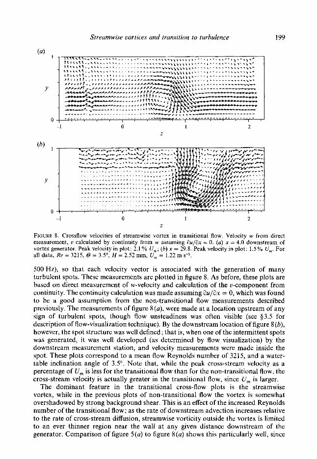
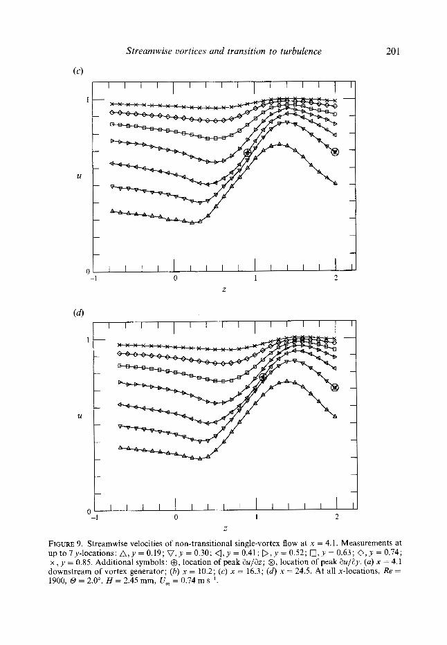
FIGURE 9. Streamwise velocities of non-transitional single-vortex flow at x = 4.1. Measurements at up to 7y-locations: A , y = 0.19; ' J , y = 0.30; 4 , y = 0.41; D , y = 0.52; 0 , y = 0.63; 0 , y = 0.74; x , y = 0.85. Additional symbols: 0, location of peak au/az; 0 , location of peak au/ay. (a) x = 4.1 downstream of vortex generator; (b) x = 10.2; ( c ) x = 16.3; ( d ) x = 24.5. At all x-locations, Re = 1900, 0=2 .0" , H=2.45mm, lJm=0.74ms-'.

202 J . M . Hamilton and F. H. Abernathy

A

0 0.2 0.4 0.6 0.8 1 .o

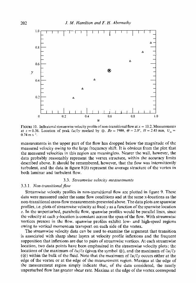
FIGURE 10. Inflexional streamwise velocity profile of non-transitional flow at x = 10.2. Measurements at z = 0.36. Location of peak au/ay marked by 0. Re = 1900, 0 = 2.0", H = 2.45 mm, Urn = 0.74 m s-l.

U

measurements in the upper part of the flow has dropped below the magnitude of the measured velocity owing to the large frequency shift. It is obvious from the plot that the measured velocities in this region are meaningless. Nearer the wall, however, the data probably reasonably represent the vortex structure, within the accuracy limits described above. It should be remembered, however, that the flow was intermittently turbulent, and the data in figure 8(b) represent the average structure of the vortex in both laminar and turbulent flow.

3.3 . Streamwise velocity measurements 3.3.1. Non-transitionaljlow

Streamwise velocity profiles in non-transitional flow are plotted in figure 9. These data were measured under the same flow conditions and at the same x-locations as the non-transitional cross-flow measurements presented above. The data plots are spanwise profiles, i.e. plots of streamwise velocity at fixed y as a function of the spanwise location z. In the unperturbed, parabolic flow, spanwise profiles would be parallel lines, since the velocity at each y-location is constant across the span of the flow. With streamwise vortices present in the flow, spanwise profiles exhibit low- and high-speed regions owing to vertical momentum transport on each side of the vortex.

The streamwise velocity data can be used to examine the argument that transition is associated with sharp shear layers at velocity profile inflexions and the frequent supposition that inflexions are due to pairs of streamwise vortices. At each streamwise location, two data points have been emphasized in the streamwise velocity plots: the locations of the maximum of au/az (given the symbol @), and the maximum of a u p y (0) within the bulk of the fluid. Note that the maximum of au/ay occurs either at the edge of the vortex or at the edge of the measurement region. Maxima at the edge of the measurement region simply indicate that, of the data considered, the nearly unperturbed flow has greater shear rate. Maxima at the edge of the vortex correspond

0.8

203

- I l l l l l ~ l l l ~ l l l A- - -

- - A - -

0.4

Y

A

0.2 A t

A

A J l I l l l l l 1 l l l l l l l I l l I

0 0.2 0.4 0.6 0.8 1 .o U

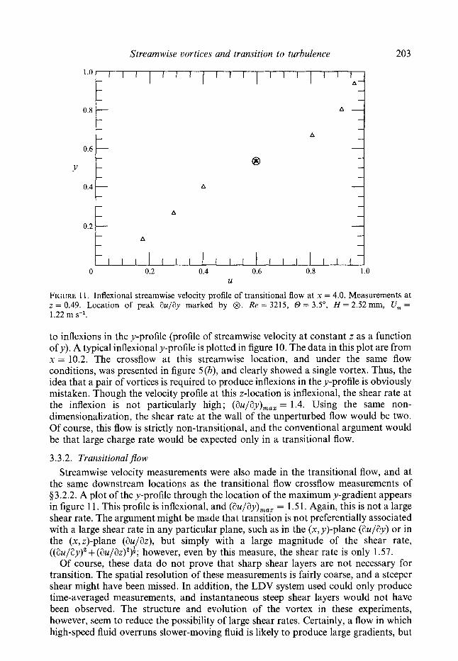
FIGURE 11. Inflexional streamwise velocity profile of transitional flow at x = 4.0. Measurements at z = 0.49. Location of peak marked by 0. Re = 3215, 0 = 3.5", H = 2.52 mm, Urn = 1.22 m s-l.

to inflexions in the y-profile (profile of streamwise velocity at constant z as a function of y) . A typical inflexional y-profile is plotted in figure 10. The data in this plot are from x = 10.2. The crossflow at this streamwise location, and under the same flow conditions, was presented in figure 5 (b), and clearly showed a single vortex. Thus, the idea that a pair of vortices is required to produce inflexions in the y-profile is obviously mistaken. Though the velocity profile at this z-location is inflexional, the shear rate at the inflexion is not particularly high; (au/~y),,, = 1.4. Using the same non- dimensionalization, the shear rate at the wall of the unperturbed flow would be two. Of course, this flow is strictly non-transitional, and the conventional argument would be that large charge rate would be expected only in a transitional flow.

3.3.2. Transitional flow Streamwise velocity measurements were also made in the transitional flow, and at

the same downstream locations as the transitional flow crossflow measurements of 43.2.2. A plot of the y-profile through the location of the maximumy-gradient appears in figure 1 1. This profile is inflexional, and (au/ay),,, = 1.5 1. Again, this is not a large shear rate. The argument might be made that transition is not preferentially associated with a large shear rate in any particular plane, such as in the (x,y)-plane (au/C)y) or in the (x,z)-plane (au/az), but simply with a large magnitude of the shear rate, ((i3u/ay)2 + (au/i3z)2))"; however, even by this measure, the shear rate is only 1.57.

Of course, these data do not prove that sharp shear layers are not necessary for transition. The spatial resolution of these measurements is fairly coarse, and a steeper shear might have been missed. In addition, the LDV system used could only produce time-averaged measurements, and instantaneous steep shear layers would not have been observed. The structure and evolution of the vortex in these experiments, however, seem to reduce the possibility of large shear rates. Certainly, a flow in which high-speed fluid overruns slower-moving fluid is likely to produce large gradients, but

204

20 - -

- 2 1 1 l 1 1 1 1 1 1 1 1 1 1 1

0 10 20 30 X

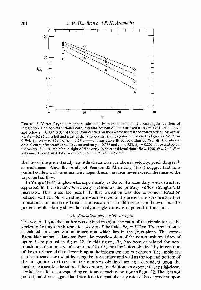
FIGURE 12. Vortex Reynolds numbers calculated from experimental data. Rectangular contour of integration. For non-transitional data, top and bottom of contour fixed at Ay = 0.221 units above and below y = 0.337. Sides of the contour centred on the z-value nearest the vortex centre, Az varies: A, Az = 0.296 units left and right of the vortex centre (same contour as plotted in figure 7); V, Az = 0.394; 0, Az = 0.493; 0, Az = 0.591. -, linear curve fit to logarithm of Re,; 0 , transitional data. Contour for transitional data centred on y = 0.356 and z = 0.628. Ay = 0.201 above and below the vortex, Az = 0.192 left and right of the vortex. Non-transitional data: Re = 1900, 0 = 2.0", H = 2.45 mm. Transitional data: Re = 3200, 0 = 3.5", H = 2.52 mm.

the flow of the present study has little streamwise variation in velocity, precluding such a mechanism. Also, the results of Pearson & Abernathy (1984) suggest that in a perturbed flow with no streamwise dependence, the shear never exceeds the shear of the unperturbed flow.

In Yang's (1987) single-vortex experiments, evidence of a secondary vortex structure appeared in the streamwise velocity profiles as the primary vortex strength was increased. This raised the possibility that transition was due to some interaction between vortices. No such structure was observed in the present measurements, either transitional or non-transitional. The reason for the difference is unknown, but the present results clearly show that only a single vortex is required for transition.

3.4. Transition and vortex strength The vortex Reynolds number was defined in (6) as the ratio of the circulation of the vortex to 271 times the kinematic viscosity of the fluid, Re, = r/271v. The circulation is calculated on a contour of integration which lies in the (y,z)-plane. The vortex Reynolds numbers calculated from the crossflow data of the non-transitional flow of figure 5 are plotted in figure 12. In this figure, Re, has been calculated for non- transitional data on several contours. Clearly, the circulation obtained by integration of the experimental data depends upon the integration contour chosen. The ambiguity can be lessened somewhat by using the free-surface and wall as the top and bottom of the integration contour, but the numbers obtained are still dependent upon the location chosen for the sides of the contour. In addition, an exponential spatial-decay law has been fit to corresponding contours at each x-location in figure 12. The fit is not perfect, but does suggest that the calculated spatial decay rate is also dependent upon


the contour chosen for calculation of the circulation. The increasing values of Re, at each x-location, and the decreasing spatial decay rates in figure 12 correspond to larger integration contours.

The in figure 12 corresponds to the circulation calculated for transitional data. While measurements were made for transitional data at two x-locations, the quality of the downstream data is too poor to make meaningful circulation measurements. The circulation shown is calculated for a single contour. The circulation was calculated on additional contours, but had the curious property of changing little for several contours clearly within the vortex, but decreasing for increasing contour dimensions outside the vortex. This suggests opposite signed vorticity surrounding the vortex, which would not be expected. This effect is probably due to the fact that the small velocities outside the vortex are not measured accurately by the LDV system, particularly at the large frequency shifts required for the transitional flow.

Despite the ambiguity in selection of the contour of integration for calculating Re,, one result is clear: the calculated value of Re, is greater in the non-transitional flow than the transitional flow, in apparent contradiction to the results of Yang (1987) and Suri (1988) who found that stronger vortices led to transition. This raises the question, is Re, the appropriate measure of vortex strength?

The problem with the definition Re, 7 l ' /2nv is that any background vorticity inside the contour of integration is included in the circulation calculation, even though this additional vorticity is not properly part of the vortex. In the present case, the streamwise vortex in the non-transitional flow is surrounded by streamwise vorticity produced by the vortex generator, but which did not roll-up as part of the vortex. There is significant circulation in this background shear, relative to the vortex, and the circulation overestimates the strength of the vortex. In the data for a transitional flow, the background shear is much less, and the circulation calculation gives a value which better represents the actual vortex strength.

A streamwise vortex and a simple crossflow shear differ in that the vortex can transport streamwise momentum normal to the wall; the crossflow shear only transports momentum parallel to the wall. In most flows, the gradients of streamwise momentum are greater normal to the wall than parallel to the wall. Thus, the streamwise vortex acts to rearrange the distribution of the streamwise momentum of the flow while any crossflow shear has relatively little effect. A useful alternative definition of the strength of the vortex would quantify the potential of the vortex for wall-normal transport of streamwise momentum, while ignoring spanwise transport. Such a definition would differentiate vortices from shear in a physically useful way.

One possible alternative definition would be to consider only the wall normal velocity in the calculation of circulation

Tr 2 vj-ds, - f (7)

where the contour of integration again lies in the (y, z)-plane, and j is the unit vector in the y-direction. The factor of 2 in (7) approximately corrects for the contribution of wk-ds in the normal definition of circulation (equation (5)) . The correction would be exact for an axisymmetric vortex if the contour were square or axisymmetric and concentric with the vortex. The associated vortex Reynolds number would be

- F Re =-.

- 2nv When this definition is used, the strength of the non-transitional and transitional


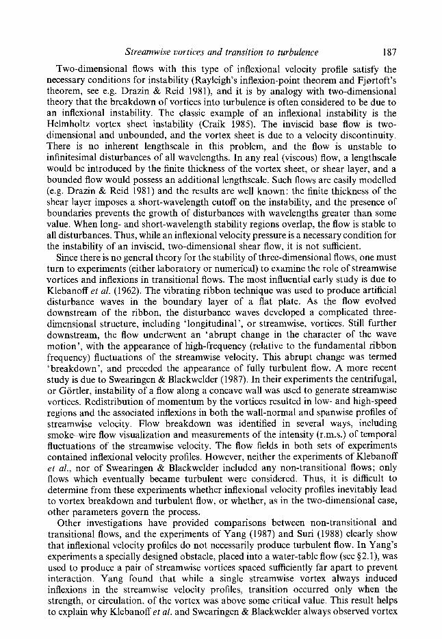
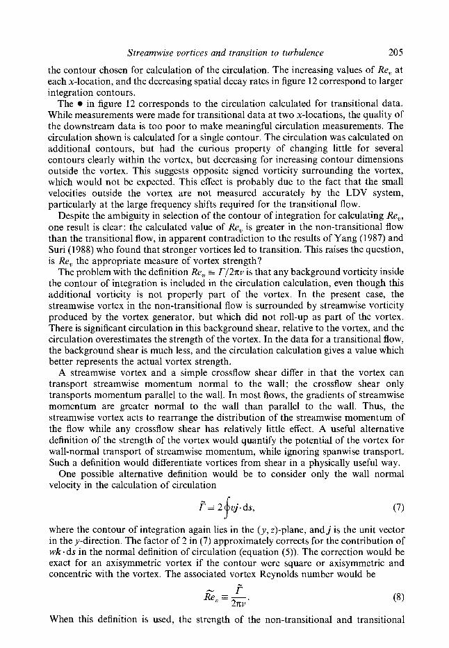
FIGURE 13. Stable flow on water table, viewed from above. The flow direction is from left to right. Generator in upper left of photograph. Only visible structures in flow are capillary waves produced by flow over the generator. Division lengths are 1 cm. Re = 2400, 0 = 2.0".

vortices calculated on similarly sized, nearly square contours become Re, = 3.4 and 10.3, respectively. The two definitions of vortex Reynolds numbers produce nearly the same values in the transitional case, reflecting the fact that there is little background vorticity to inflate the conventionally calculated value of Re,. In the non-transitional case, background vorticity produces a value of Re, which is more than twice the value obtained when only wall-normal velocity is considered. These values are calculated from the same contour used in the data of figure 12 for the transitional case, and a contour centred on y = 0.337, z = 0.757, with top and bottom 0.221 units from the centre and left-hand and right-hand sides 0.197 units from the centre for the non- transitional case.

This alternative definition of vortex strength clearly discriminates between vortex strength and vorticity, but still retains an ambiguity associated with the selection of an integration contour. A more attractive approach might be to look directly at the redistribution of streamwise momentum by the vortex. Yang (1987) used this method to deduce vortex strength because equipment limitations prevented him from measuring the crossflow directly. The present study, however, has produced much more information than was available to Yang, and a new numerical flow model was developed to take advantage of this additional information. The fundamental assumption of the numerical model was that the spatial development of the streamwise vortex could be modelled as temporal development. Thus, the model flow had no streamwise dependence @/ax of any quantity is zero) but did vary with time. The a priori motivation for this type of model rested on the observation that the structure of the vortex changes little downstream of the generator; in the non-transitional flow data


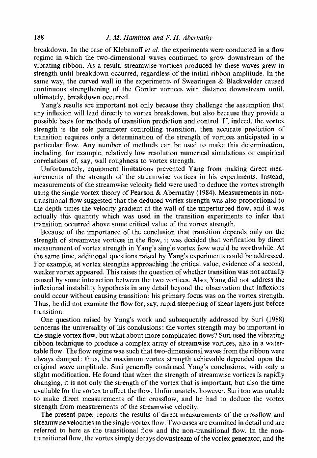
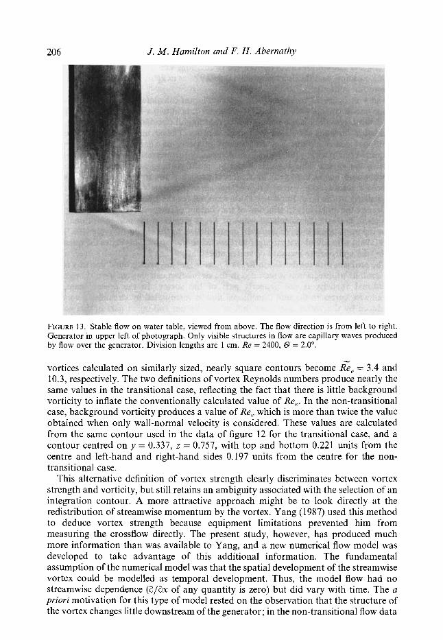
FIGURE 14. Unstable flow on water table, viewed from above. The flow direction is from left to right. Generator visible at upper left of photograph. Distortion of free-surface downstream of generator caused by flow disturbance. Disturbance subsequently decays downstream. Division lengths are 1 cm. Re = 2150, 0 = 4.0".

of figure 5, it is primarily the downstream decay of the crossflow that distinguishes one x-location from another. Unfortunately, this model did not reproduce the details of the flow adequately. Experimental data from the non-transitional flow (sg3.2.1 and 3.3.1) were used as the initial condition for the model, and it was hoped that the temporal evolution of the model would duplicate the spatial evolution of the experiment when an appropriate 'advection' velocity was used to convert time into space. It was found that the required velocity was much faster than any velocity occurring in the flow. In addition, when idealized vortices were used for initial conditions, the redistribution of momentum was found to be very dependent on the initial structure of the vortex. Thus, this particular flow model did not provide a means of separating the vortex from the background vorticity in the experimental data in any adequate or unambiguous way.

3.5. Transition and streamwise vortices ' 3.5.1. Single streamwise vortex

The free-surface of the water table is particularly useful as a flow-visualization tool. When a white screen is placed beneath the glass surface of the water table and illuminated from above, bright and dark regions corresponding to small free-surface curvature effects are observed. Convex regions (i.e. regions in which the centre of curvature lies on the liquid side of the interface) produce bright spots, while concave regions cause shadows. This visualization technique was used in the photographs of figures 13-16. The flow illumination (electronic flash) was inclined downstream at about 30" from vertical to reduce reflection of the light source from the free surface.

208 J . M. Hamilton and F. H. Abernathy

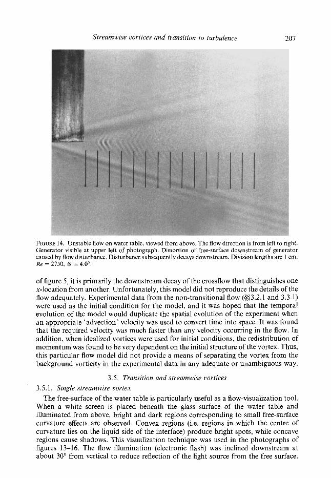
FIGURE 15. Unstable flow on water table, viewed from above. The flow direction is from left to right. Generator visible at upper left of photograph. Flow conditions same as previous figure, but this disturbance continues to grow into a turbulent spot downstream. Division lengths are 1 cm. Re = 2150, 0 = 4.0".

The flow rate and water-table inclination angles in these photographs were varied to produce the desired phenomena; there is no systematic variation of a single flow parameter from photo to photo.

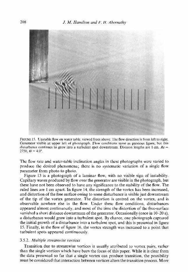
Figure 13 is a photograph of a laminar flow, with no visible sign of instability. Capillary waves produced by flow over the generator are visible in the photograph, but these have not been observed to have any significance to the stability of the flow. The ruled lines are 1 cm apart. In figure 14, the strength of the vortex has been increased, and distortion of the free surface owing to some disturbance is visible just downstream of the tip of the vortex generator. The distortion is centred on the vortex, and is observable nowhere else in the flow. Under these flow conditions, disturbances appeared almost continuously, and most of the time the distortion of the free-surface vanished a short distance downstream of the generator. Occasionally (once in 10-20 s), a disturbance would grow into a turbulent spot. By chance, one photograph captured the initial growth of a disturbance into a turbulent spot, and this is presented in figure 15. Finally, in the flow of figure 16, the vortex strength was increased to a point that turbulent spots appeared continuously.

3.5.2. Multiple streamwise vortices

Transition due to streamwise vortices is usually attributed to vortex pairs, rather than the single vortices which have been the focus of this paper. While it is clear from the data presented so far that a single vortex can produce transition, the possibility must be considered that interaction between vortices alters the transition process. More


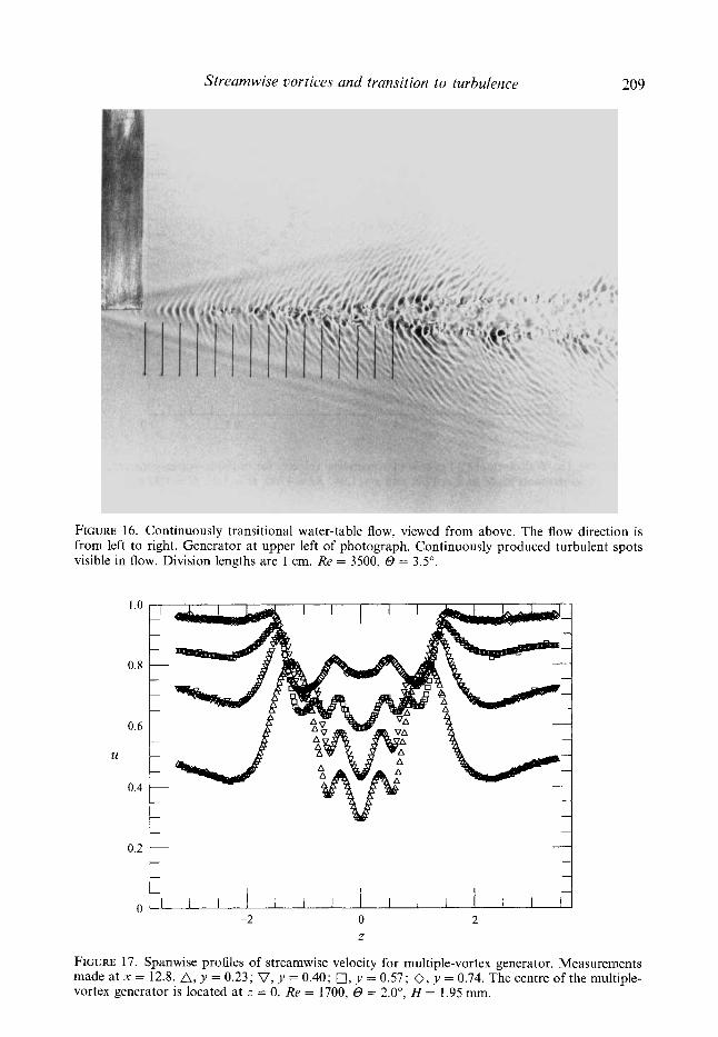
FIGURE 16. Continuously transitional water-table flow, viewed from above. The flow direction is from left to right. Generator at upper left of photograph. Continuously produced turbulent spots visible in flow. Division lengths are 1 cm. Re = 3500, 0 = 3.5".

1 .o

0.8

0.6

U

0.4

0.2

0 -2 0 2

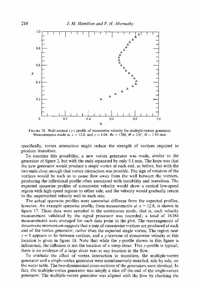
FIGURE 17. Spanwise profiles of streamwise velocity for multiple-vortex generator. Measurements made at x = 12.8. A, y = 0.23; V, y = 0.40; 0, y = 0.57; 0, y = 0.74. The centre of the multiple- vortex generator is located at z = 0. Re = 1700, @ = 2.0", H = 1.95 mm.


-I A A

0.6

Y

0.4

A A

A A A A A A A A A A

A A 1

d A A

A

0 0.2 0.4 0.6 0.8 1 .o U

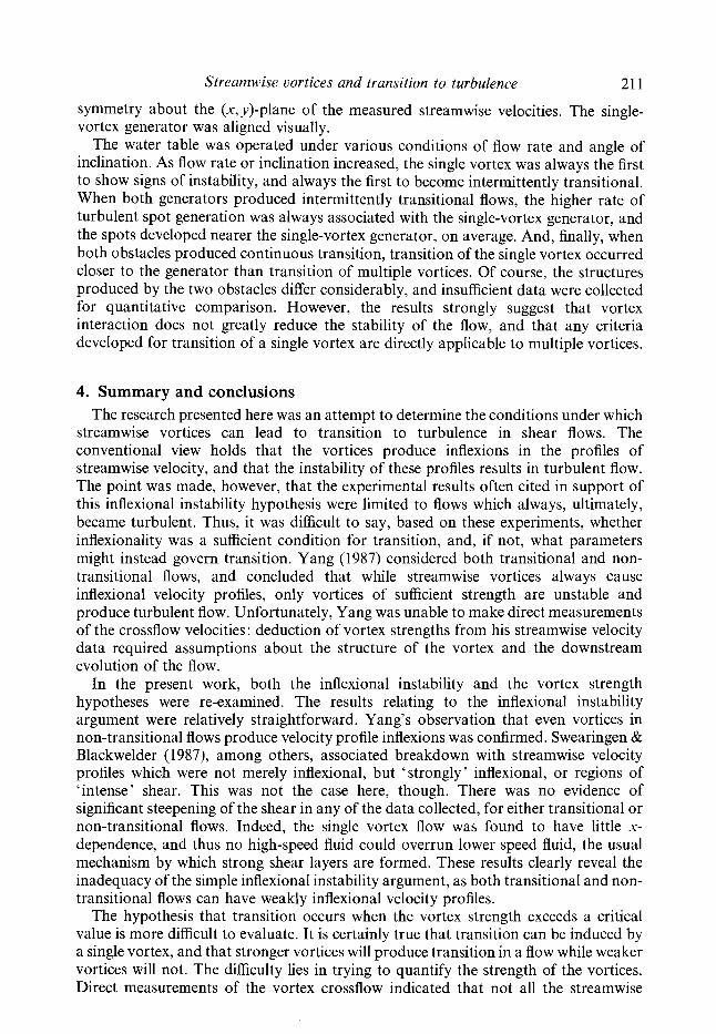
FIGURE 18. Wall-normal ( y - ) profile of streamwise velocity for multiple-vortex generator. Measurements made at x = 12.8, and z = 1.04. Re = 1700, 0 = 2.0", H = 1.95 mm.

specifically, vortex interaction might reduce the strength of vortices required to produce transition.

To examine this possibility, a new vortex generator was made, similar to the generator of figure 2, but with the ends separated by only 5.1 mm. The hope was that the new generator would produce a single vortex at each end, as before, but with the two ends close enough that vortex interaction was possible. The sign of rotation of the vortices would be such as to cause flow away from the wall between the vortices, producing the inflexional profile often associated with instability and transition. The expected spanwise profiles of streamwise velocity would show a central low-speed region with high-speed regions to either side, and the velocity would gradually return to the unperturbed velocity well to each side.

The actual spanwise profiles were somewhat different from the expected profiles, however. An example spanwise profile, from measurements at x = 12.8, is shown in figure 17. These data were sampled in the continuous mode, that is, each velocity measurement validated by the signal processor was recorded; a total of 16384 measurements were averaged for each data point in the plot. The rearrangement of streamwise momentum suggests that a pair of streamwise vortices are produced at each end of the vortex generator, rather than the expected single vortex. The region near z = 1 appears to lie between vortices, and a y-traverse of streamwise velocity at this location is given in figure 18. Note that while the y-profile shown in this figure is inflexional, the inflexion is not the location of a steep shear. This y-profile is typical; there is no evidence of a large shear rate at any location in the flow.

To evaluate the effect of vortex interaction in transition, the multiple-vortex generator and a single-vortex generator were simultaneously installed, side by side, on the water table. The two-dimensional cross-sections of the generators were identical. In fact, the multiple-vortex generator was simply a slice off the end of the single-vortex generator. The multiple-vortex generator was aligned with the flow by checking the

Streamwise vortices and transition to turbulence 21 1

symmetry about the (x, y)-plane of the measured streamwise velocities. The single- vortex generator was aligned visually.

The water table was operated under various conditions of flow rate and angle of inclination. As flow rate or inclination increased, the single vortex was always the first to show signs of instability, and always the first to become intermittently transitional. When both generators produced intermittently transitional flows, the higher rate of turbulent spot generation was always associated with the single-vortex generator, and the spots developed nearer the single-vortex generator, on average. And, finally, when both obstacles produced continuous transition, transition of the single vortex occurred closer to the generator than transition of multiple vortices. Of course, the structures produced by the two obstacles differ considerably, and insufficient data were collected for quantitative comparison. However, the results strongly suggest that vortex interaction does not greatly reduce the stability of the flow, and that any criteria developed for transition of a single vortex are directly applicable to multiple vortices.

4. Summary and conclusions The research presented here was an attempt to determine the conditions under which

streamwise vortices can lead to transition to turbulence in shear flows. The conventional view holds that the vortices produce inflexions in the profiles of streamwise velocity, and that the instability of these profiles results in turbulent flow. The point was made, however, that the experimental results often cited in support of this inflexional instability hypothesis were limited to flows which always, ultimately, became turbulent. Thus, it was difficult to say, based on these experiments, whether inflexionality was a sufficient condition for transition, and, if not, what parameters might instead govern transition. Yang (1987) considered both transitional and non- transitional flows, and concluded that while streamwise vortices always cause inflexional velocity profiles, only vortices of sufficient strength are unstable and produce turbulent flow. Unfortunately, Yang was unable to make direct measurements of the crossflow velocities : deduction of vortex strengths from his streamwise velocity data required assumptions about the structure of the vortex and the downstream evolution of the flow.

In the present work, both the inflexional instability and the vortex strength hypotheses were re-examined. The results relating to the inflexional instability argument were relatively straightforward. Yang’s observation that even vortices in non-transitional flows produce velocity profile inflexions was confirmed. Swearingen & Blackwelder (1 987), among others, associated breakdown with streamwise velocity profiles which were not merely inflexional, but ‘ strongly’ inflexional, or regions of ‘intense’ shear. This was not the case here, though. There was no evidence of significant steepening of the shear in any of the data collected, for either transitional or non-transitional flows. Indeed, the single vortex flow was found to have little x- dependence, and thus no high-speed fluid could overrun lower speed fluid, the usual mechanism by which strong shear layers are formed. These results clearly reveal the inadequacy of the simple inflexional instability argument, as both transitional and non- transitional flows can have weakly inflexional velocity profiles.

The hypothesis that transition occurs when the vortex strength exceeds a critical value is more difficult to evaluate. It is certainly true that transition can be induced by a single vortex, and that stronger vortices will produce transition in a flow while weaker vortices will not. The difficulty lies in trying to quantify the strength of the vortices. Direct measurements of the vortex crossflow indicated that not all the streamwise

212 J. M . Hamilton and F, H. Abernathy

vorticity present near a streamwise vortex ‘rolls up’ into the vortex. The remaining, ‘background’, vorticity appears to play no role in transition, but is difficult to separate from the vorticity actually associated with the vortex when calculating the vortex strength. In addition, the contour on which the strength, or circulation, is calculated is always somewhat ambiguous in regions of diffuse vorticity.

The difficulty in unambiguously identifying the vortices which will lead to transition indicates that the problem is still not well understood. The parameter(s) which governs vortex-induced transition is probably more complicated than simply the strength of the vortex. Further analysis will be required to understand adequately the nature of the single-vortex instability.

Nevertheless, the present results may be of useful, if limited, application. While an exact critical vortex strength has not been identified, it is clear that flows containing streamwise vortices of vortex Reynolds number much less than about ten are unlikely to become turbulent, while vortices of strength much greater than ten probably will produce transition. Thus, it may be possible to use the strength of streamwise vortices as the basis of a scheme to predict whether any given flow (e.g. flow in a pipe with rough walls) will become turbulent. Specific data, such as the location of transition would, however, remain beyond our ability to predict.

We particularly wish to thank Drs Anil K. Suri, Zhongmin Yang and Joseph D. Myers for many helpful discussions.

R E F E R E N C E S BATCHELOR, G. K. 1967 An Introduction to Fluid Dynamics. Cambridge University Press. BERTSCHY, J. R. 1979 Laminar and turbulent boundary layer flows of drag reducing solutions. PhD

CHIN, R. W. 1981 Stability of flows down an inclined plane. PhD thesis, Division of Applied

CRAIK, A. D. D. 1985 Wave Interactions and Fluid Flows. Cambridge University Press. DRAZIN, P. H. & REID, W. H. 1981 Hydrodynamic Stability. Cambridge University Press. HAMILTON, J. M. 1991 Streamwise vortices and transition to turbulence. PhD thesis, Division of

Applied Sciences, Harvard University. HORSTMANN, K. H., QUAST, A. & REDEKER, G. 1990 Flight and wind-tunnel investigations of

boundary-layer transition. J. Aircraft 27, 146. KLEBANOFF, P. S., TIDSTROM, K. D. & SARGENT, L. M. 1962 The three-dimensional nature of

boundary-layer instability. J. Fluid Mech. 12, 1. LIGHTHILL, M. J. 1963 In Laminar Boundary Layers (ed. L. Rosenhead), pp. 46-113. Clarendon

(reprinted by Dover). OBARA, C. J. & HOLMES, B. J. 1985 Flight-measured laminar boundary-layer transition phenomena

including stability theory analysis. N A S A TP-2417. PEARSON, C. F. & ABERNATHY, F. H. 1984 Evolution of the flow field associated with a streamwise

diffusing vortex. J . Fluid Mech. 146, 271. PRESS, W. H., FLANNERY, B. P., TEUKOLSKY, S. A. ~VETTERLING, W. T. 1986 Numerical Recipes: the

Art of Scientijc Computing. Cambridge University Press. SABERSKY, R. H., ACOSTA, A. J. & HAUPTMANN, E. G. 1971 Fluid Flow: A First Course in Fluid

Mechanics, 2nd edn. Macmillan. SURI, A. K. 1988 Streamwise vortices in shear flow transition. PhD thesis, Division of Applied

Sciences, Harvard University. SWEARINGEN, J. D. & BLACKWELDER, R. F. 1987 The growth and breakdown of streamwise vortices

in the presence of a wall. J. Fluid Mech. 182, 255. YANG, Z. 1987 A single streamwise vortical structure and its instability in shear flow. PhD thesis,

Division of Applied Sciences, Harvard University.

thesis, Division of Applied Sciences, Harvard University.

Sciences, Harvard University.

Documents

Streamwise vortices and transition to turbulence