Curved two-stream turbulent mixing layers: three-dimensional structure and streamwise evolution

J. Fluid Mech. (1994), vol. 270, pp . I-SO Copyright 0 1994 Cambridge University Press

Curved two-stream turbulent mixing layers : three- dimensional structure and streamwise evolution

By MICHAEL W. PLESNIAK‘, RABINDRA D. MEHTA’ A N D JAMES P. JOHNSTON3

School of Mechanical Engineering, Purdue University, West Lafayette, IN 47907-1288, USA Department of Aeronautics and Astronautics, JIAA Stanford University, Stanford,

CA 94305-4035, USA and Fluid Mechanics Laboratory, NASA Ames Research Center, Moffett Field, CA 94035-1000, USA

Department of Mechanical Engineering, Stanford University, Stanford, CA 94305-3030, USA

(Received 12 May 1993 and in revised form 1 December 1993)

The three-dimensional structure and streamwise evolution of two-stream mixing layers at high Reynolds numbers (Re, M 2.7 x lo4) were studied experimentally to determine the effects of mild streamwise curvature (6/R < 3 %). Mixing layers with velocity ratios of 0.6 and both laminar and turbulent initial boundary layers, were subjected to stabilizing and destabilizing longitudinal curvature (in the Taylor-Gortler sense). The mixing layer is affected by the angular momentum instability when the low-speed stream is on the outside of the curve, and it is stabilized when the streams are reversed so that the high-speed stream is on the outside. In both stable and unstable mixing layers, originating from laminar boundary layers, well-organized spatially stationary streamwise vorticity was generated, which produced significant spanwise variations in the mean velocity and Reynolds stress distributions. These vortical structures appear to result from the amplification of small incoming disturbances (as in the straight mixing layer), rather than through the Taylor-Gortler instability. Although the mean streamwise vorticity decayed with downstream distance in both cases, the rate of decay for the unstable case was lower. With the initial boundary layers on the splitter plate turbulent, spatially stationary streamwise vorticity was not generated in either the stable or unstable mixing layer. Linear growth was achieved for both initial conditions, but the rate of growth for the unstable case was higher than that of the stable case. Correspondingly, the far-field spanwise-averaged peak Reynolds stresses were significantly higher for the destabilized cases than for the stabilized cases, which exhibited levels comparable to, or slightly lower than, those for the straight case. A part of the Reynolds stress increase in the unstable layer is attributed to ‘extra’ production through terms in the transport equations which are activated by the angular momentum instability. Velocity spectra also indicated significant differences in the turbulence structure of the two cases, both in the near- and far-field regions.

1. Introduction Since plane turbulent mixing layers are often encountered in practical situations,

considerable effort has been directed toward understanding their structure and development. Following Townsend (1976), it is generally believed that after a sufficient development distance, all mixing layers should achieve a self-similar condition which is fully independent of the initial conditions. However, it is well known that considerable scatter exists in the published data on the streamwise development of free-

2 M. W. Plesniak, R. D. Mehta and J . P. Johnston

shear layers, leading to many areas of confusion (Birch & Eggers 1973; Rodi 1975). The main reason for this confusion, or, more precisely, lack of agreement, between different experiments, it that mixing layers are very sensitive to small changes in their initial and operating conditions, the effects of which often persist for relatively long distances downstream (Bell & Mehta 1993). In particular, even the structure of mixing layers generated from the relatively simple two-dimensional geometries turns out to be rather complex with a strong dependence on initial conditions (Ho & Huerre 1984).

Since the late 1970s, experimental studies have shown that mixing layers originating from laminar initial boundary layers develop a secondary structure in the form of pairs of counter-rotating streamwise vortices (Konrad 1976; Bernal & Roshko 1986; Lasheras, Choi & Maxworthy 1986). These structures are superimposed on the familiar primary structure consisting of large-scale (Kelvin-Helmholtz) spanwise vortices (Brown & Roshko 1974). The earlier results suggested that the streamwise (‘rib’) vortices first formed in the braid region connecting adjacent spanwise vortices, with their location determined by the strength and position of weak incoming disturbances fed from the initial boundary layers. Jimenez (1983) obtained time-averaged velocity measurements which showed strong spanwise ‘wrinkles’, thus confirming earlier beliefs that the streamwise structures could be spatially stationary. Some results also suggested that the scale, and hence spacing, of the streamwise vortices increased with downstream distance. Huang & Ho (1990) obtained velocity measurements which showed that the spanwise spacing of the streamwise structures doubled after a pairing of adjacent spanwise vortices. These studies and other related work on this topic (e.g. Lasheras & Choi 1988; Jimenez 1988; Jimenez, Cogollos & Bernal 1985) were all confined to the near-field region, and mostly conducted at relatively low Reynolds numbers.

The presence and role of streamwise structures in a mixing layer at high Reynolds number (Re, z 2.9 x lo4) were recently investigated by Bell & Mehta (1989a, 1992). A plane, two-stream mixing layer was generated, with a velocity ratio of 0.6, and laminar initial boundary layers which were nominally two-dimensional. Measurements of the mean streamwise vorticity indicated that small spanwise disturbances originating upstream in the boundary-layer flow were initially amplified just downstream of the first spanwise roll-up, leading to the formation of stationary streamwise vortices. The mean vorticity first appeared in clusters containing vorticity of both signs, but further downstream, it re-organized to form counter-rotating pairs. The vortex structures were then found to grow in size with downstream distance, the spanwise wavelength associated with them scaling approximately with the local mixing-layer vorticity thickness. These vortical structures also weakened downstream, with the maximum mean vorticity diffusing approximately as X-1.5. As a result, the mixing layer appeared to be nominally two-dimensional in the far-field region.

Amongst the parameters that are known to affect mixing-layer behaviour are the splitter plate geometry (Dziomba & Fiedler 1985), velocity ratio (Mehta & Westphal 1986; Mehta 1991), confining boundaries (Wood & Bradshaw 1984; Gibson & Younis 1983), initial momentum thickness (Hussain & Zedan 1978) and the free-stream turbulence intensity (Pate1 1978). In the present study, it was necessary to interchange the high- and low-speed sides to create stabilizing and destabilizing curvature in the same test section. Because of the sensitive nature of mixing layers, the effects of this minor change in initial conditions were documented (Plesniak, Bell & Mehta 1992, 1993) to ensure that the effects of curvature, and not initial condition dependence, were being studied. The interchange between the two sides resulted in small changes in the initial boundary-layer properties, and an interchange between the perturbations

Curved two-siream turbulent mixing layers 3

present in the boundary layers. The results showed that while the exact positions and shapes of the individual mean streamwise vortical structures were somewhat different for the two cases, their overall description and statistical behaviour, including their reorganization and decay was very similar. As a result, in the far-field, both mixing layers achieved similar structure, yielding comparable growth rates, Reynolds stress distributions and spectral content. The only notable differences were in the near-field Reynolds stress (peak) levels which were attributed to differences in the details of the initial spanwise vortex roll-up.

Another important parameter is the state (laminar or turbulent) of the initial boundary layers (Browand & Latigo 1979; Bell & Mehta 1990). For one thing, with both initial boundary layers tripped (turbulent), organized (spatially stationary) streamwise vorticity is not observed, and consequently the mixing layer appears to be two-dimensional in the mean (Bell & Mehta 1990). Furthermore, for two-stream mixing layers it has been found that the growth rate for the untripped (laminar) case is higher than that of the tripped case (Oster, Wygnanski & Fiedler 1977; Browand & Latigo 1979; Browand & Troutt 1985; Bell & Mehta 1990). However, the asymptotic peak Reynolds stress levels, as well as the mean velocity and turbulence profiles, appear comparable for the two cases (Browand & Latigo 1979; Bell & Mehta 1990). Bell & Mehta (1990) attributed the higher growth rate for the untripped case to the presence of spatially stationary streamwise vortices, which provide additional entrainment.

It is well known that an inviscid instability occurs in any curved flow where the angular momentum decreases away from the centre of curvature (Bradshaw 1973). A popular and widely studied example of this is the concave boundary layer, where the instability results from the no-slip condition at the wall. The instability leads to the quasi-inviscid generation of (Taylor-Gortler) streamwise roll cells which appear in counter-rotating streamwise pairs with an approximate spanwise wavelength equivalent to twice the boundary-layer thickness (Hoffmann, Muck & Bradshaw 1985; Barlow & Johnston 1988; Johnson & Johnston 1989). Substantial increases in the Reynolds stress levels and large changes in the turbulence structure occur, induced either directly by the curvature acting on the fine-scale turbulence or indirectly by the large-scale roll cells (Smits & Wood 1985). These roll cells also lead to increased skin friction and heat transfer. On the other hand, the boundary-layer flow over a convex wall experiences a stabilizing effect such that three-dimensional effects and Reynolds stress levels are suppressed (Gillis & Johnston 1983; Muck, Hoffmann & Bradshaw 1985). Pre-existing turbulence is attenuated without significant changes in the boundary-layer turbulence structure in the wall-layer region. A mixing layer with curvature in the streamwise direction is expected to experience similar effects; the layer is subjected to a destabilizing effect if the low-speed stream is on the outside of the curve and a stabilizing effect if it is on the inside of the curve.

Since the pioneering experimental work of Margolis & Lumley (1965), Wyngaard (1967) and Wyngaard et al. (1968) on the effects of longitudinal curvature on turbulent mixing layers, it is well known that curvature affects Reynolds stress production and turbulence transport. These studies showed that destabilizing curvature enhances Reynolds stress production, while stabilizing curvature inhibits production. Castro & Bradshaw (1976) investigated a highly curved single-stream mixing layer subjected to strong stabilizing curvature and found that the Reynolds stresses, triple products, energy dissipation rate and other statistical quantities decreased below the straight layer values. A ‘fairly thin shear layer’ approximation was put forth in order to help numerical modellers account for the effects of the extra rates of strain due to curvature. Gibson & Rodi (1981) implemented these suggestions in their calculation

4 M . W. Plesniak, R. D. Mehta and J . P. Johnston

utilizing a Reynolds-stress closure model. Their model was able to reproduce the suppression of turbulence by stabilizing curvature in accordance with the experimental observations of Castro & Bradshaw.

In all of the studies described above, the effects of strong curvature (SIR + 10%) were investigated. A highly curved mixing layer is formed, for example, by allowing a jet to impinge on a wall so as to turn the flow through 90" (Castro & Bradshaw 1976). The shear layer on the boundary of the jet is turned abruptly and grows by entraining ambient fluid. In contrast, a mildly curved mixing layer may be formed by merging two parallel fluid streams of different speed and gently curving the test section walls downstream of the point of merger, the trailing edge of the splitter plate. Gibson & Younis (1983) investigated a single-stream turbulent mixing layer subjected to mildly destabilizing streamwise curvature (S/R < 8 %). They found a 9 YO increase in the spreading rate and a 14 YO increase in maximum shear stress over the values measured in a straight layer.

The subject of streamwise curvature effects on mixing-layer structure has received limited attention. Wang (1 984) studied the structure of mildly curved two-stream mixing layers by performing a systematic investigation of the interaction of various instability mechanisms due to velocity ratios, curvature effects, and density effects. His results revealed that for a curved mixing layer with uniform (constant) density, the large spanwise structures that form from the Kelvin-Helmholtz instability are weakened by the Taylor-Gortler instability. The rate of vortex pairing appeared to be reduced for the curved mixing layers, although the growth rate (based on the visual thickness) of the unstable mixing layer was greater than that of the stable case. Destabilizing curvature was also found to promote three-dimensionality in the flow. In addition, Wang showed that a density difference across the mixing layer activates structures associated with the Rayleigh-Taylor instability. These structures have the finest scale and the greatest degree of three-dimensionality, a desirable situation for enhanced mixing.

Plesniak & Johnston (1989a, b) investigated the role of mild curvature (d/R < 4 %) on the structure and development of a low-Reynolds-number (Re, E 400) two-stream mixing layer developing from laminar boundary layers ( y o = V, /U, = 0.5). Flow visualization and three-component laser Doppler velocimetry (LDV) measurements showed that streamwise vortices were present in all cases, but they were strongest in the unstable case. The unstable layer developed to a state with fine-scale mixing and enhanced turbulence transport much earlier (in space) than the stable layer. Large Taylor-Gortler 'rollers' similar to those present in concave boundary layers (cf. Barlow & Johnston 1988) were not observed in the unstable mixing layer. The maximum primary Reynolds shear stress in the unstable layer was approximately twice that of the stable-layer value at most measuring stations, and the secondary shear stresses indicated the presence of the strongest streamwise vortices in the unstable layer. In addition, the growth rate of the unstable shear-layer vorticity thickness was twice that of the stable layer. The growth rate of the straight mixing layer (used for reference) was lower than that of the unstable layer, and higher than that of the stable layer. Triple correlations and higher-order moments showed that the unstable layer exhibited enhanced turbulence transport with maxima of the triple products in the unstable case two to four times as large as the corresponding values in the stable layer. In particular, the lateral transport of turbulence was greatly enhanced in the unstable layer.

So, while the issues regarding the effects of curvature on plane mixing-layer structure and streamwise development have been addressed in some of these previous

Curved two-stream turbulent mixing layers 5

investigations, several areas of confusion still remain. First, the Reynolds number in the studies of Plesniak & Johnston (1989~7, b) was rather low, and the establishment of far-field structural similarity was therefore questionable. The effects of initial conditions (boundary-layer state) on curved mixing-layer structure have not been previously investigated. In the unstable mixing layer, the role of the Taylor-Gortler effect, if present, has not been clearly established. The effect of systematic streamwise curvature on the amplification of the 'natural' streamwise (rib) vorticity has also not been investigated. In particular, is the production of the streamwise vorticity affected by curvature? How is the evolution of the vorticity affected by the two types of curvature? As shown in previous studies, the effect of stabilizing curvature is to reduce the amount of mixing and Reynolds-stress production, while destabilizing curvature results in faster shear-layer growth, enhanced mixing and elevated levels of Reynolds stresses. However, the mechanisms through which these effects are introduced are not well understood.

Accordingly, the first objective of the present study was to establish quantitatively the effects of stabilizing and destabilizing curvature on the three-dimensional structure of two-stream mixing layers. The second objective was to establish the effects of curvature on the global properties of the mixing layer such as the growth rate and development of the Reynolds stresses. The studies were to be conducted at relatively high Reynolds numbers, and at a sufficient downstream distance to ensure that the effects of initial conditions had decayed. Four different cases were investigated during the course of this research program - two layers (stable and unstable) each originating from laminar (untripped) and turbulent (tripped) initial conditions.

2. Experimental techniques The experiments were performed in a mixing-layer wind tunnel, the details of which

are given in Bell & Mehta (1989b, 1992). The wind tunnel consists of two separate legs, each independently driven by a centrifugal blower connected to a variable-speed motor. Upon exiting the blowers, air passes through wide-angle diffusers, through flow conditioners, and then through an 8 : 1 two-dimensional contraction. The two streams merge downstream of the sharp trailing edge of a tapered splitter plate. The included angle of the splitter plate is approximately I", and the trailing edge is about 0.25 mm thick. The curved test section (figure 1) has a fixed mean radius of curvature, R, of 305 cm, giving a maximum 6 / R of less than 3 %, and measures 36 cm in the cross- stream direction, 91 cm in the spanwise direction and 366 cm in length (measured along the centreline arc). Note that the constant curvature is applied immediately from the splitter-plate trailing edge, and extends to the end of the test section. One wall was slotted for probe access and allowed streamwise pressure gradient adjustment. In all the cases studied, the wall was adjusted to give a nominally zero streamwise pressure gradient (the streamwise variation in free-stream velocity was less than 1 %).

In the present experiments the two sides of the wind tunnel were run at free-stream velocities of 9 and 15 m s-', initially giving a mixing layer with a velocity difference, U, = U,- U, = 6 m s-l, and a nominal velocity ratio, r, = &/U, = 0.6 ( A = [( 1 - r J / ( 1 + r,)] = 0.25). These velocities were set just upstream of the tip of the splitter plate, before curvature is imposed. Note that for curved flows, the moment of momentum and not the velocity remains constant in the potential flow. Therefore, the velocity difference was defined as U, = [(RU),-(RU),]/R, and the velocity ratio was defined as r = (RU),/(RU), which was necessarily slightly different for the stable and unstable cases, since the initial velocity ratio was matched at X = 0. The typical local

6 M . W. Plesniak. R. D . Mehta and J . P. Johnston

I \ (Stable configuration depicted)

Two-dimensional I contraction / f

FIGURE 1 . Schematic of curved test section. All dimensions in cm.

Condition u, 899 6

(m s-l) (cm) (cm) Laminar boundary layers

High-speed side, stable case 15.0 0.40 0.053 Low-speed side, stable case 9.0 0.44 0.061 High-speed side, unstable case 15.0 0.39 0.054 Low-speed side, unstable case 9.0 0.44 0.055

High-speed side, stable case 15.0 0.92 0.093 Low-speed side, stable case 9.0 0.98 0.119 High-speed side, unstable case 15.0 0.94 0.101 Low-speed side, unstable case 9.0 0.95 0.099

TBLE 1. Initial boundary-layer properties

Turbulent boundary layers

525 362 532 322

920 700

1000 596

2.52 2.24 2.29 2.61

1.41 1.32 1.44 1.49

velocity ratio was 0.57 for the stable cases and 0.62 for the unstable cases. For the stabilizing curvature case, the stream on the outside of the curved section was operated at a free-stream velocity of 15 m s-l while that at smaller radius was run at 9 m s-l. The high- and low-speed sides were interchanged to produce the destabilizing case in the same test section. In all cases, the free-stream velocities were held constant to within 1 YO during a typical run lasting 2-4 h. The measured streamwise turbulence intensity (u'/ U,) in the free stream was approximately 0.15 YO and the transverse levels (d/ U, and w'/U,) were less than 0.05 YO. The mean core-flow was found to be uniform to within 0.5% and cross-flow angles were less than 0.25" (Bell & Mehta 1989b).

The experiments were performed with both laminar and turbulent boundary layers on the splitter plate. To create the turbulent initial conditions, the boundary layers were tripped with two-dimensional cylindrical rods (1.5 mm in diameter) glued across the span of the splitter plate about 15 cm upstream of the trailing edge. The boundary- layer properties for each set of initial conditions are tabulated in table 1. The tabulated values represent the average values computed from profiles measured at five different


spanwise locations. The spanwise variation of the tabulated properties was less than 2 Yo, indicating the absence of any strong three-dimensional disturbances in the boundary layers on the splitter plate.

Measurements were made using a cross-wire probe mounted on a three-dimensional traverse, operated by Dantec 55M 10 anemometers, and linked to a fully automated data acquisition and reduction system controlled by a MicroVax I1 computer. At a given streamwise location, the measurements were made along the local radius, with the probe tip aligned with the local streamline. The cross-wire probe (Dantec Model 55P5 1) consisted of 5 pm platinum-plated tungsten sensing elements approximately 1 mm long, and separated by approximately 1 mm. The probe was calibrated statically in the potential core of the flow (between the mixing layer and the wall boundary layer) assuming a ‘cosine-law’ response to yaw, with the effective angle determined by calibration. The analogue signals were filtered (low-pass at 30 kHz), DC offset, and amplified ( x 10) before being fed into a fast Tustin sample-and-hold A/D converter with 15 bit resolution and a multiplexer for connection to the computer. The wind- tunnel reference velocity (used for normalizing the data) and temperature were also acquired through the A/D converter. A temperature correction was applied to the hot- wire measurements to account for ambient temperature drift during the course of a data run. Individual statistics were averaged over 5000 samples obtained at a rate of 1500 samples per second, for a total sampling time of 3.33 seconds per point. The number of samples and sampling times were chosen based on an optimization between the need to minimize overall data acquisition time (to minimize hot-wire drift) and the desire to obtain adequate convergence of the mean velocities and turbulence statistics.

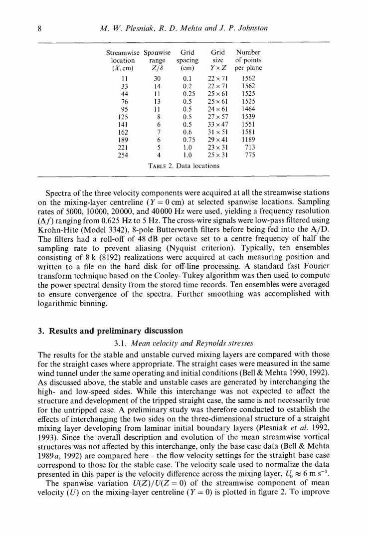
Measurements were made in cross-sectional (Y , Z)-planes with the rotatable cross- wire probe set in two orientations (uv and uw). This method yielded all three components of mean velocity, five independent components of the Reynolds stress tensor (u/wl was not measured) and selected higher-order products. Measurements were made at eleven streamwise stations within the test section. Details of the measurement grids are given in table 2, the numbers quoted are those for the untripped unstable case, but those for the other cases were not much different.

An error analysis, based on calibration accuracy and repeatability of measurements, indicates that mean streamwise velocity measurements with the cross-wire are accurate to within 2 YO, while mean cross-stream velocities are accurate to within 7 YO. Reynolds normal stress measurements are accurate to within 5 Yo, and shear stresses are accurate to within 1&15%0.

The measurements were corrected for mean streamwise velocity gradient (a U/a Y and aU/aZ) effects-details of the correction scheme are given in Bell & Mehta (1989~). The streamwise component of mean vorticity (52,) was computed using a central difference numerical differentiation of the measurements of the velocity components V and W. The overall circulation per vortical structure (0 was determined from the surface integral of the mean streamwise vorticity field over the cross-flow plane,.t with vorticity levels less than 20 % of the maximum value being set to zero in order to provide immunity from ‘noise’. The integration was performed over a rectangular ‘box’ on the measured grid that fully encompassed each identified vortex (that containing at least two closed vorticity contours, with the spacing of the contour levels equivalent to 10 % of (Q,)ma,). The mean streamwise vorticity measurements were repeatable to within about 15-20 % and the circulation measurements were repeatable to within about 20-25 %.

t The circulation was also computed by integrating along a contour r = $c V . ds, and typically agreed to within about 5 % with that given by the surface integral.

8 M. W. Plesniak, R. D. Mehta and J. P. Johnston

Streamwise Spanwise location range (X,cm) z/s

11 30 33 14 44 11 76 13 95 11

125 8 141 6 162 7 189 6 22 1 5 254 4

Grid spacing

(cm) 0.1 0.2 0.25 0.5 0.5 0.5 0.5 0.6 0.75 1 .0 1 .0

Grid size

Y X Z

22 x 71 22 x 71 25 x 61 25 x 61 24 x 61 27 x 57 33 x47 31 x51 29x41 23 x 31 25 x 31

TABLE 2. Data locations

Number of points per plane

1562 1562 1525 1525 1464 1539 1551 1581 1189 713 775

Spectra of the three velocity components were acquired at all the streamwise stations on the mixing-layer centreline ( Y = 0 cm) at selected spanwise locations. Sampling rates of 5000, 10000, 20000, and 40000 Hz were used, yielding a frequency resolution (An ranging from 0.625 Hz to 5 Hz. The cross-wire signals were low-pass filtered using Krohn-Hite (Model 3342), 8-pole Butterworth filters before being fed into the A/D. The filters had a roll-off of 48 dB per octave set to a centre frequency of half the sampling rate to prevent aliasing (Nyquist criterion). Typically, ten ensembles consisting of 8 k (8192) realizations were acquired at each measuring position and written to a file on the hard disk for off-line processing. A standard fast Fourier transform technique based on the Cooley-Tukey algorithm was then used to compute the power spectral density from the stored time records. Ten ensembles were averaged to ensure convergence of the spectra. Further smoothing was accomplished with logarithmic binning.

3. Results and preliminary discussion 3.1. Mean velocity and Reynolds stresses

The results for the stable and unstable curved mixing layers are compared with those for the straight cases where appropriate. The straight cases were measured in the same wind tunnel under the same operating and initial conditions (Bell & Mehta 1990,1992). As discussed above, the stable and unstable cases are generated by interchanging the high- and low-speed sides. While this interchange was not expected to affect the structure and development of the tripped straight case, the same is not necessarily true for the untripped case. A preliminary study was therefore conducted to establish the effects of interchanging the two sides on the three-dimensional structure of a straight mixing layer developing from laminar initial boundary layers (Plesniak et al. 1992, 1993). Since the overall description and evolution of the mean streamwise vortical structures was not affected by this interchange, only the base case data (Bell & Mehta 19890, 1992) are compared here - the flow velocity settings for the straight base case correspond to those for the stable case. The velocity scale used to normalize the data presented in this paper is the velocity difference across the mixing layer, U, % 6 m s-l.

The spanwise variation U ( Z ) / U ( Z = 0) of the streamwise component of mean velocity ( U ) on the mixing-layer centreline ( Y = 0) is plotted in figure 2. To improve


-+ X= 11 cm +, 33 cm

+ 44cm 16cm

_jc_ 9Scm 125cm

h 0

I I

. h

tu b W

+ X = 141 cm + 162 cm

-h- 189cm --+- 221 cm + 254cm

-15.0 -5.0 5.0 15.0 -15.0 -5.0 5.0 15.0

(cm> (cm) FIGURE 2. Spanwise variation of mean streamwise velocity: (a) untripped unstable case;

(b) untripped stable case; ( c ) tripped unstable case; ( d ) tripped stable case.

readability, the origin of each curve is successively shifted upward with increasing downstream distance. For the untripped curved mixing layers, the ‘wrinkles’ in the streamwise velocity are attributable to the presence of spatially stationary streamwise vortices (see Huang & Ho 1990; Bell & Mehta 1992). In the unstable mixing layer, the spanwise variation appears only quasi-periodic at first, but by X = 76 cm, a more regular and periodic variation is exhibited. The spanwise variation in U (peak-to-peak) is 13 O/O at the first station, increasing to about 15 YO at X = 3 3 4 4 cm, after which it decreases, but still exhibits a variation of about 5 % at the last two stations. In comparison, the straight mixing layer also exhibited similar variations which became very regular by X = 78 cm (Bell & Mehta 1992). In that study, a variation of 6 % was measured at X = 8 cm, increasing to a maximum of about 10 YO at X = 37-57 cm, after which it decreased again. In the far-field region (X = 250 cm), the streamwise velocity was nearly constant across the span of the mixing layer, indicating mean two- dimensionality. The stable mixing layer exhibits somewhat lower (- 8 YO) spanwise variation in U compared to the corresponding unstable mixing layer at X = 11 cm. However, the degree of variation in U decreases almost monotonically further downstream, becoming much smaller than that measured in the unstable case. All of the stations downstream of X = 95 cm exhibit nearly constant distributions of U across the stable mixing-layer span. In both cases, the spanwise wavelength of the wrinkles

10 M . W. Plesniak, R. D. Mehta and J. P. Johnston

Contour Value 1 0.0050 2 - - - - - - 0.0075 3- - - 0.0100 4 - - 0.0125 5- 0.0150 6 0.0250 7 - - - - - - 0.0350

...........

...........

(4 Untripped unstable case

0.5 E

w - 0 5 x -1 5

- 0

-3.5 -2.5 -1.5 -0.5 0.5 1 5 2 5 3.5

5 , (b)

I n

W o } x

-5 ‘ I -20 -15 -10 -5 0 5 10 15 20

Untripped stable case I I

0.5

- 0.5

-1.51 -3.5 -2.5 -1.5 -0.5 0.5 1.5 2.5 3.5

5 I I

0

-5 -20 -15 -10 -5 0 5 10 15 20

5 - 5 -

0 -

-5 -5 -

E 2, 0 - x

-

-10 1 ‘ -101 I -20 -15 -10 -5 0 5 10 15 20 -20 -15 -10 -5 0 5 10 15 20

z (cm) z ( 4 FIGURE 3. Primary shear stress ( n / V , ” ) contours: (a) X = 11 cm; (b) X = 76 cm; (c) X = 189 cm.

increases with increasing streamwise distance. This is consistent with the notion that the wavelength associated with pairs of counter-rotating streamwise vortices scales approximately with the local mixing-layer vorticity thickness (Jimenez 1983 ; Bernal & Roshko 1986; Bell & Mehta 1992).

The spanwise variation of U for both tripped cases is presented in figures 2(c) and 2(d). It is clearly evident that the variation for both cases, at all streamwise locations is minimal. The same result was also reported for the tripped straight case by Bell & Mehta (1 990). This implies that spatially stationary vorticity is not produced for the tripped cases, and, furthermore, that the imposition of curvature does not change the mixing-layer mean structure, at least in terms of producing Taylor-Gortler-type streamwise vorticity. Although this is true for the present mild curvature, this does not necessarily mean that large-scale roll cells will not be generated for stronger curvature. This possibility is further discussed in $4.1.

The distribution of the Reynolds stresses was also affected by curvature and the initial conditions. The primary shear stress (m) contours for the untripped curved cases at three stations are presented in figure 3. At X = 11 cm, local ‘islands’ of are observed in the unstable case, whereas the stable case exhibits a more conventional distribution, albeit with some small local peaks. The maximum levels for the two cases,

Curved two-stream turbulent mixing layers I 1

though, are comparable. Further downstream, at X = 76 cm, the contours for the stable case appear almost two-dimensional and exhibit lower peak levels compared to the unstable case. The contours for the unstable case have the characteristic regular wrinkles seen in the mean velocity contours. Although the distortion is reduced in the unstable case at X = 189 cm, the stable case contours still appear more two- dimensional. The disparity in peak levels between the two cases is maintained through to this station. Not surprisingly, the contours for both the curved tripped cases (not presented here) exhibited a nominally two-dimensional behaviour, although the peak levels in the unstable case were consistently _ _ higher at all streamwise locations. The contours for the normal stress components ( U ’ ~ , U ’ ~ , and z) are not presented here, since their behaviour (owing to the effects of curvature and initial conditions) is similar to that of the primary shear stress. In particular, the trend of the higher stress levels and greater degree of three-dimensionality in the unstable layer is exhibited by all of the normal stresses.

3.2. Streamwise vortex structure Since the spanwise variation in mean velocity and Reynolds stresses is attributed to the presence of spatially stationary streamwise vortices, some of the vortex properties are now examined for the untripped curved cases. Contours of mean streamwise vorticity (LIZ/ U,, cm-l) at the four streamwise locations closest to the splitter plate are compared in figure 4 for the unstable and stable cases. Different contour levels had to be selected for the two cases since the vorticity magnitudes for the stable case, at least downstream of the first station, were significantly lower. At the first station ( X = 11 cm), positive and negative mean streamwise vorticity appears in clusters in both the stable and unstable mixing layers. The clusters are similar to those observed in the straight cases (Plesniak et al. 1992), although they are not as clearly defined. At this location, the maximum vorticity levels in the stable case range from -0.5 to 0.6, and in the unstable case from -0.8 to 0.7. The vorticity in both cases decays with increasing downstream distance, as reflected by the lower maximum levels. At X = 33 cm for the unstable case, the mean streamwise vorticity appears to be organized in a nearly regular row of alternating-signed structures, whereas in the stable case, no such organization is exhibited, and the maximum mean vorticity levels are significantly lower. Further downstream at X = 44 cm, in the unstable case the streamwise vorticity appears in an array with alternating signs and contour levels between -0.15 and 0.2. Note the increase in physical lengthscale of the vortical structures, and hence the spacing between them, between the X = 33 and 44 cm stations. Also, there is a relatively large variation in the strengths of the individual vortices across the span. In the stable case at this location, the mean streamwise vorticity again appears to be randomly distributed across the span of the mixing layer, and its magnitude is bounded by the relatively low contour levels of -0.06 and 0.22. At X = 76 cm, the mean vorticity in the unstable case is now aligned in a regular array of streamwise vortices? of alternating sign (counter-rotating pairs), and again, no evidence of the structure appears in the corresponding plot for the stable mixing layer. Note that apparent structures at the edge of the stable mixing layer are remnants of noise introduced by the numerical

t One may question the use of the nomenclature vortex to describe the structures which have regions of positive and negative mean streamwise vorticity as shown here in figure 4. The maximum values of the circulatory velocity components, Vand W, in a cross-stream plane are only 0.02 to 0.04 times the average convection velocity, 12 m s-’, at X = 76 cm. Such a slowly rotating flow does not possess attributes of a true vortex. For example, it would show no detectable low pressure core. Such a structure might be better described as a vortical structure, but we follow convention in this paper and retain the term vortex used in earlier works by Bell & Mehta (1992).


Contour Value 1 0.20

0.15 2 - - - _ - - 0.10 3 ---

4 - - 0.05 5 - 0.02 6 - 0.02 7 - 0.05 8 -- - -0.10 9-- -0.15

10 - - 0.20

...........

...........

Untripped unstable case (a)

2 ‘ I -4 -3 -2 -1 0 1 2 3 4

-4 ‘ -8 -6 -4 -2 0 2 4 6 8


0.06 2 - - - - - - 0.04 3 ---

4 - - 0.02 5- 0.01 6 -0.01

- 0.02 7 - - - - - - - 0.04 8 ---

9 - - - 0.06 10 - - 0.08

...........

...........

Untripped stable case 1

0

-1

1 -4 -3 -2 -1 0 1 2 3 4

-4 -8 -6 -4 -2 0 2 4 6 8

4

“Z. - * _ _ - 1 - 6 - 4 - 2 0 2 4 6 8 - 8 - 6 - 4 - 2 0 2 4 6 8

-15 -10 -5 0 5 10 15 -15 -10 -5 0 5 10 15

( 4 (cm) FIGURE 4. Mean streamwise vorticity (QJ U, cm-l) contours: (a) X = 11 cm; (b) X = 33 cm;

(c) X = 44 cm; (d ) X= 76 cm.

differencing scheme and the contouring routine. Vorticity levels of 0.01 represent the lower limit of accuracy inherent in the differentiation - the background noise associated with this scheme.

Corresponding contour plots for the cases originating from tripped initial conditions show no evidence of organized streamwise vorticity, and are not presented here. A comparison of streamwise vorticity contours between the tripped and untripped


2 - h

v 0 - h

-2


0.006 2 - - - - - _ 0.004 3 ---

4-- 0.002 5 - 0.001 6 -0.001

- 0.002 7 - - - - - - - 0.004 8 _ _ _

9-- - 0.006

...........

...........

10 - -0.008

2 -

0 -

- -2 -

Contour Value ........... 1 0.0030 0.0020 2 - - - - - - 0.0010 3 ---

4 -- 0.0005 5 - 0.0002 6 - 0.0002

- 0.0005 7 _ _ _ _ - - 8 --- -0.0010 9 -- - 0.0020

10 - -0.0030

...........

Untripped unstable case Untripped stable case (4

4 , I 4 , I

-4 1 ' -41 I - 8 - 6 - 4 - 2 0 2 4 6 8 - 8 - 6 - 4 - 2 0 2 4 6 8

I 5 , I

n

W E 0 - 0 x

-5 I I -15 -10 -5 0 5 10 15 -15 -10 -5 0 5 10 15

J -51 I -15 -10 -5 0 5 10 15 -15 -10 -5 0 5 10 15

z (cm) z (4 FIGURE 5. Secondary shear stress (u"/U,") contours: (a) X = 33 cm; (b) X = 76 cm;

(c) X = 95 cm.

straight mixing layers was presented by Bell & Mehta (1990). The tripped curved mixing-layer streamwise vortex structure is similar to that reported for the straight layer. It is particularly significant that no streamwise vorticity is observed in the tripped unstable case. This confirms the implications of the mean velocity results that the destabilizing curvature does not generate strong (spatially stationary) streamwise vorticity through the Taylor-Gortler mechanism.

Contour plots of the secondary Reynolds shear stress (u" /U,") are presented in figure 5 at three streamwise locations - note again the different contour levels for the stable and unstable cases. As was shown by Bell & Mehta (1992) for the straight mixing layer, there is again an excellent correspondence between the contours of u" and mean streamwise vorticity. Using the Reynolds stress transport equation for u", they showed that this secondary shear stress is generated primarily through the production term, -W'2aU/aZ. Note that W'2 is relatively high along the mixing-layer centreline and aU/aZ, which is generated by the streamwise vortices, has a maximum at the


I I I I , , I l l I 5 x 100 10’ 102

x (cm>

FIGURE 6. Streamwise development of peak mean vorticity. -, untripped straight case; 0, untripped unstable case; 0, untripped stable case.

location of the vortex centre. As the mean streamwise vorticity decays with streamwise distance, aU/aZ is reduced and so is the production of m, as exhibited in figure 5. Hence, an excellent correlation between the streamwise vorticity and the secondary shear stress is produced. In fact, since is more accurately measured than 9,, it is a more precise representation of the streamwise vortex structure. At X = 33 cm, the contours corresponding to positive and negative levels of uIw/ form an array across the span of the unstable mixing layer, with a spanwise spacing of approximately 1.0 cm. A similar, less well-defined array is observed in the stable mixing layer at this location, with a spacing of approximately 1.5 cm. The greater spacing in the stable case implies that the vorticity in this case grows and diffuses faster than that in the unstable case. At X= 76 cm, the spanwise spacing between the peaks has increased to approximately 2.5 cm in both the stable and unstable mixing layers. However, the peaks in the unstable layer are more clearly defined and higher in magnitude by a factor of about five. By the next station, at X = 95 cm, the levels in the unstable case have not dropped much, although the spacing between the peaks has increased to about 2.75 cm. However, in the stable case, the levels and organization of m have dropped to a point where it may be considered to be just background ‘noise’. These results clearly show that a regular array of spatially stationary streamwise vortices is generated in both cases, only the vortices in the stable case grow and diffuse faster.

The streamwise development of the evaluated (global) streamwise vortex properties are presented in figures 6-8. Note that the data for the stable case are only plotted out to X = 76 cm, since the vorticity levels at subsequent stations are too low to allow discrimination of the streamwise vortices from the background noise. The data for the tripped cases are also not included, since no significant mean streamwise vorticity was measured in those cases.

The magnitude of the peak mean vorticity (52, /~) ,az is obtained by averaging the maximum absolute values of all the streamwise vortices at each streamwise location - the vortices are identified or verified as noted above in $2. As is evident in figure 6, the initial level of mean streamwise vorticity for the unstable case is comparable to that of the straight case. At the first station (X = 11 cm), the level for the stable case is lower by a factor of about two, but it appears possible to extrapolate back to the same value as the straight case in the very near field (note that the first measuring station for the

Curved two-stream turbulent mixing layers 15 - 0.3

8 W

G 0 .d

I I I

...

... ....

. .

'......"' ,. . , '0..

L'' ~ L,. ....... .* ... ... ...*....... ..

- 9

0 50 100 150 200

x (cm) FIGURE 7. Streamwise development of average streamwise vortex circulation. -, untripped

straight case; 0 , untripped unstable case; 0, untripped stable case.

6 I I I

0 50 100 150 200

x (cm) FIGURE 8. Streamwise development of streamwise vortex spacing. -, untripped straight case;

0, untripped unstable case; 0, untripped stable case.

curved cases is at X = 11 cm, while that for the straight layer is at X = 8 cm). The main difference between the two curved cases is in the near-field ( X < 30 cm) decay rates. The decay rate for the unstable case is initially lower than that for the straight case, while that for the stable layer is much greater. In the far field, the decay rates for the curved cases are approximately the same as that for the straight layer, which follows a X-'.5 decay. As a consequence of the difference in the near-field decay rates, the magnitude of the peak streamwise vorticity for the unstable case at the downstream stations is clearly higher than that for the straight case, whereas that of the stable case is significantly lower.

The overall characterization of a vortex is best given by its circulation. The circulation of any streamwise vortical structure observed in the present study should remain approximately constant, unless it is altered by a specific mechanism. The circulation, r/ t.&, for each identified vortex is evaluated as described above in $2, and the absolute values are then averaged over all the vortices at a given streamwise station. The average circulation per vortex for all three cases remains relatively constant with


temporary increases and decreases (figure 7). The temporary increases may be due to amalgamation of like-signed vortices (Bell & Mehta 1992), whereas the temporary decreases may be attributed to the interaction of opposite-signed vortices - viscous annihilation of vortices of the same strength or viscous amalgamation of vortices of unequal strength (Rogers & Moser 1993). The mean circulation level for the unstable case (- 0.18 cm) is clearly higher than that for the straight case ( - 0.12 cm), while that for the stable case is distinctly lower ( N 0.03 cm) - the differences are significant since they are higher than the estimated measurement uncertainty of 2&25% for this quantity. Some of the difference in circulation levels between the three cases may be due to errors introduced by the ‘boxing’ procedure used to define the region of integration. Obviously, in the cases where the vortices are relatively weak, the defined box may not encompass the entire vortex, since the vorticity magnitudes on the outskirts drop to levels equivalent to the noise in the vorticity measurement scheme. Therefore, the actual circulation may be underestimated by this procedure. However, since the large differences in r between the three cases are apparent even in the near field (X = 33 cm), where the vorticity levels are relatively high, we believe that the differences are real, and a consequence of the effects of curvature.

The spacing between the streamwise vortices, obtained by dividing the measured span by the number of identified vortices, is plotted in figure 8. The spacing seems to increase in a stepwise fashion, especially for the straight and unstable cases. In the near- field region, the spacing increases faster in the stable case, and slightly slower in the unstable case, compared to the straight case. This confirms the notion that the mean streamwise structures in the stable case grow and diffuse faster than those in the straight case. Conversely, those in the unstable case diffuse less rapidly, thus maintaining their strength. Results from previous studies have suggested that the local increase in spacing (and scale) occurs during a pairing of the spanwise vortices (Jimenez et al. 1985; Huang & Ho 1990), although an increase is not always observed at every pairing location (Bell & Mehta 1992). Recent results from a direct numerical simulation of a temporally evolving mixing layer have shown that the details of the scale change are strongly dependent on the amplitudes of the initial three-dimensional disturbances (Rogers & Moser 1993). In the present study, the local increases in spacing seem to occur close to locations where the average circulation also increases. This correspondence confirms earlier beliefs (Bell & Mehta 1992) that at least one mechanism for the increase in spacing could be the amalgamation of like-signed streamwise vortices, the others being amalgamation or annihilation of opposite-signed vortices (Rogers & Moser 1993). Clearly, for vortex amalgamation to occur, vortices in a single row (of counter-rotating pairs) would have to rotate out of the row so that two like-signed vortices end up closer together. Such a rotation is feasible because of the large variation in vortex strength along the span at a given station. Thus, the motion due to spanwise mutual self-induction would be such that the orderly row of vortices becomes irregular, thus allowing like-signed vortices to occupy adjacent positions.

3.3. Velocity spectra The effects of curvature and initial conditions are clearly apparent relatively early in the mixing-layer development. These effects are reflected in both the mean flow, in terms of the streamwise vorticity, and also in the Reynolds stress distributions. In order to further investigate the curved mixing-layer structure, velocity spectra were also measured. The u-, u- and w-component spectra measured at X = 11 cm for all four curved cases are presented in figure 9. All of the spectra presented in this paper are plotted in logarithmic coordinates, and the power spectral density (Eii) is normalized

x 10-2

10-2

10-5

10-7

10-9

x 10-2

10-2

10-3

10-4

10-5

10-7

E,, 0 2


I I I I I I I I I I I I I I I l l 1 I I I I I I l l

lo-*

10-2

10-3

10-4

10-5

10-6

10-7

10-8

10-9 10' 102 103 104

Frequency (Hz) FIGURE 9. Spectral measurements on mixing-layer centreline ( Y = Z = 0) at X = 11 cm for all four curved cases: (a) u-component; (b) v-component ; (c) w-component. -, untripped unstable case ; ---, untripped stable case; ---, tripped unstable case; . . . , tripped stable case.


(a ) 5 x 10-2

10-3

10-4

10-5

10-6

10-7

10-8

10-2

E,, 0 2

10-9 t I I I I I l l l l I I I I I I I I I I I I I 1 1 1

(b) 5 x

10-2

10-3

10-4

10-5 E,, 0 2

10-6

10-7

10-8

10-9

(4 5

E,, 0 2

x 10-2

10-2

10-3

10-4

10-5

10-6

10-7

10-8

10-9 10' 102 103

Frequency (Hz) 104

FIGURE 10. Spectral measurements on mixing-layer centreline ( Y = 2 = 0) at X = 76 cm for all four curved cases: (a) u-component; (b) v-component; (c) w-component. See figure 9 for legend.

by the variance (r2). For all three velocity components, the untripped unstable case is the only one which exhibits the characteristic fundamental peak a t f x 630 Hz, caused by the Kelvin-Helmholtz vortex roll-up. The fundamental peak is followed by some higher harmonics. The untripped stable case has a broadband distribution, quite

Curved two-stream turbulent mixing luyers 19

(a) 5 x

10-2

10-3

10-4

10-5 E,, 0 2

10-7

10-9

(b) 5 x 10-2

10-3

10-4

10-5

10-6

10-7

10-8

E,, 0 2

10-9

(c) 5 x 10-2 t

10-2

10-3

10-4

10-5

10-7

10-8

1n-9 t I I I I I I I I I I I I I I I I I I I I I I 1 1 1 1 -"

10' 102 103 Frequency (Hz)

104

FIGURE 1 1. Spectral measurements on mixing-layer centreline ( Y = 2 = 0) at X = 254 cm for all four curved cases: (a) u-component; (b) o-component; (c) w-component. See figure 9 for legend.

similar to those for the two tripped cases (which are comparable). So for the tripped cases, there does not seem to be much effect of the curvature (stabilizing versus destabilizing) on the spectral content of the mixing layer, at least in the very near field. However, the untripped cases are affected significantly, even at this early stage of their


- - ....... .... -1cm -. 3 cm 0 cm - -

I I I I I I l l 1 $ I I L I 1 1 1 1 I

1 (b) 5 x 10-2

I I I I I l l l l I I I I I l l l l I

c

10-6 10' 102 103

Frequency (Hz) FIGURE 12. Spectral measurements at X = 1 1 cm on mixing-layer centreline ( Y = 0) and varying spanwise locations for the untripped unstable case: (a) u-component ; (b) v-component ; (c) w- component.


development. It is worth noting that the differences are not due to changes in initial conditions - the spectra for the two straight cases (with initial conditions corresponding to the stable and unstable cases) both exhibited the fundamental and higher-order peaks (Plesniak et al. 1992, 1993). The implication of the spectral results is that the Kelvin-Helmholtz vortices are either weakened or become temporally variant in the untripped stable case as a result of the stabilizing curvature. It is also observed that the untripped stable case generates more small scales in the near field, making it comparable to the tripped cases where the smaller scales are injected directly from the turbulent boundary layers. Somewhat remarkably, the spectra for all four cases at X = 76 cm (figure 10) seem to exhibit very good collapse for all three components, and over the whole frequency range. However, at X = 254 cm in the far-field region (figure 1 l), there is clearly a ' peeling-off' of the profiles such that at the higher-frequency end, the unstable cases have more energy. By this station, there does not seem to be much effect of the initial boundary layers. Note the strong peak in the u-spectra at f z 40-50 Hz for both the stable cases.

Since large spanwise variations were noted in the Reynolds stress distributions (especially in the unstable case), spectra were measured along the mixing-layer centreline, at several different spanwise locations. The u-, v- and w-component spectra measured at X = 11 cm in the untripped unstable case (figure 12) all show the fundamental peak atf z 630 Hz followed by some higher harmonics. The 8-component spectra collapse quite well for the various spanwise locations, especially in the region of the fundamental peak. However, the spectra for the u-component and, in particular, the w-component do show some variations which are presumably due to the streamwise vortical structures - one would expect the w-component spectra to be affected the most by the streamwise vortices. The spanwise differences are not as apparent further downstream at X = 76 cm (figure 13). Adequate collapse is observed in all three components, especially for f > 100 Hz. Although relatively strong mean streamwise vorticity was measured at this station, it is presumably not strong enough (compared to the mixing-layer turbulence) to affect the spanwise spectral distributions. Bell & Mehta (1992) showed that the initial average streamwise vortex circulation was equivalent to approximately 10 O/O of the spanwise circulation.

The u-, u- and w-component velocity spectra for all streamwise locations and for all four curved cases are shown in figures 14-17. The untripped unstable spectra at the first station (figure 14) show a fundamental peak at f z 630 Hz, followed by higher harmonics in all three components. A slow increase in power spectral density magnitude is observed at the low-frequency end with increasing downstream distance, whereas the energy at the high-frequency end is reduced. Beyond X = 125 cm and for f > 100 Hz, a reasonable collapse of the profiles is observed, especially in the u- and w- component spectra. A slight hump a t f = 10-30 Hz is also apparent towards the end of the measurement domain, especially in the u- and w-spectra.

The spectra for the untripped stable case (figure 15) do not exhibit the fundamental peak corresponding to the Kelvin-Helmholtz roll-up, as discussed above. The trends further downstream are similar to those for the untripped unstable case with the energy at the low-frequency end increasing, and that at the higher end decreasing. The two main differences between the two untripped curved cases are that the spectra in the stable case do not appear to collapse in the far-field region and a distinct peak is visible atf = 30-50 Hz in all three components, although the one in the v-component data is the strongest.

The tripped unstable spectral data (figure 16) show trends similar to those for its untripped counterpart, except that the fundamental peak is noticeably absent at the


(b) 5 x 10-2

10-3

10-4

10-5 - E"" 0 2

10-6

10-7

10-9

(c) 5 x 10-2 t

10-9 t I I I I I I I I I I I I I I I I I I 1 I I I l I I 1

10' 102 103 1 0 4 Frequency (Hz)

FIGURE 13. Spectral measurements at X = 76 cm on mixing-layer centreline ( Y = 0) and varying spanwise locations for the untripped unstable case: (a) u-component; (b) u-component ; (c) w- component.


X

X = l l c m -. X = 162 cm 33cm -- 221 cm 76cm - 254 cm 125 cm

I I I I 1 I I I I I I 1 1 1 1 1 1 1 I I I 1111L

i

10-2

10-3

10-4

10-5

10-7

10-9 t- 1 I 1 I I IIII

10-8

I I I I 1 1 1 1 1 I I 1 I I I l l

10-2

10-2

10-3

10-4

10-5

10-6

10-7

10-8

1 n-9

104 1"

10' 1 0 2 103

Frequency (Hz) FIGURE 14. Spectral measurements on mixing-layer centreline ( Y = Z = 0) at all streamwise locations

for the untripped unstable case : (a) u-component ; (b) u-component ; (c ) w-component.

first station, as would be expected. The downstream trends are very similar to those observed in the untripped case with the spectra for X > 125 cm again showing good collapse for f > 100 Hz. A small hump at f = 20-40 Hz in the far-field region is also apparent in these results for the u- and w-components. The tripped stable spectra

24 M. W. Plesniak, R. D. Mehta and J. P. Johnston

-X= 11 cm --X= 1 6 2 cm. 33cm - - 2 2 1 cm- - - - - - 76 cm - 254 cm- - - 125 cm

(b) 5 x 10-Z10-2

10-3

10-42 E02 10-5

10-6

lo-’

10-g

1o-9

(4 5

Ewwo2

x 10-210-2

10-3

10-4

10-S

1om6

10-7

10-8

1om910’ 102 103 lo4

Frequency (Hz)

F IGURE 15. Spectral measurements on mixing-layer centrel ine (Y = Z = 0) at al l s treamwise locationsfor the untripped stable case: (a) u-component; (b) v-component; (c) w-component.

(figure 17) also show trends similar to its untripped counterpart with the higher energyshifting towards the low-frequency end and a lack of collapse of the profiles in the far-field region. A rather distinct peak atfz 45 Hz is clearly visible in the v-spectra at thedownstream stations.

Curved two-stream turbule*nt mixing layers 25

(4 5

E-!!!!02

@I 5

x 10-210-2

10-3

1o-4

10-5

10-6

10-7 -x=11an --X=I62cm33cm - - 2 2 1 c m

10-x 76cm - 2 5 4 c m

10-4

10-5

10-6

10-7

10-9 I- I I11111ll I I I t11111IO’ 102 103 lo4

Frequency (Hz)

FIGURE 16. Spectral measurements on mixing-layer centreline (Y = 2 = 0) at all streamwise locationsfor the tripped unstable case: (a) u-component; (b) v-component; (c) w-component.

A distinct peak at a frequency of 20-50 Hz is observed in all of the spectra, althoughit is more pronounced in the stable cases. A similar, but weaker, peak was alsoobserved in the spectra for the straight cases. It is proposed here that this low-frequency peak is due to the passage of the spanwise vortex roll-ups. The peak begins


X

(c) 5 x 10-2

10-2

10-3

Eww __ 10-5 0 2

10-6

lo-'

10-8

I I I I I I 1 1 1 I I I I I I I I I I I I I I l l

loL 102 10 104

Frequency (Hz) FIGURE 17. Spectral measurements on mixing-layer centreline ( Y = 2 = 0) at all streamwise locations

for the tripped stable case: (a) u-component; (b) u-component; (c) w-component.

to appear in the spectra for X > 162 cm, by which point it is estimated, based on Bell & Mehta's (1992) results for the straight case, that about four pairings of the spanwise vortices have occurred. This would give a vortex passage frequency of about 40 Hz with the fundamental peak at f M 630 Hz. The peaks are stronger in the stable case


probably because it has the least mean three-dimensionality (the streamwise vortices decay the fastest).

3.4. Mixing-layer thickness and maximum Reynolds stresses As shown above in 93.1, relatively large spanwise variations were observed in the mean velocity and Reynolds stress distributions, essentially in the untripped cases. Therefore, in order to obtain a more accurate representation of the behaviour of some of the global properties of the mixing layers, such as the thickness and peak Reynolds stresses, a spanwise averaging technique was applied to the data for all four cases. The spanwise averaged quantities were evaluated by dividing the measurements obtained on the cross-plane grid into individual Y-wise profiles or 'slices' through the mixing layer. The mixing-layer properties for each slice were then computed in the traditional manner. And finally, the slice-specific properties were algebraically averaged over all spanwise positions, giving a single value for each quantity. In effect, depending on the streamwise location, the properties were averaged over 30 to 70 individual spanwise profiles covering a spanwise extent of between 5 and 30 mixing-layer thicknesses (see Bell et al. 1992 for details of the spanwise averaging technique and its implications).

3.4.1. Mixing-layer thickness Two definitions of the mixing-layer thickness are used in the present study: the

thickness based on a data fit to the error function profile, and the vorticity thickness. The mixing-layer thickness (8) was determined using a two parameter fit to the error function velocity profile shape suggested by Townsend (1976) :

where U" = :( 1 + erf(r)),

The parameters S and 5 are determined by an optimization routine in the error function fit.

The mixing-layer vorticity thickness (8,) is defined by the following relation for the curved layers :

[ ( U R ) , - ( W , I [a(UR)/a YI,,, '

S, =

which reduces to the usual expression for straight mixing layers:

The mixing-layer growth for the stable, unstable and straight cases with untripped and tripped initial conditions is given in terms of S in figure 18(a) and in terms of 6, in figure 18(b). The curved cases are denoted by symbols, whereas lines are used for the reference straight cases. In both figures, all the mixing layers exhibit linear growth downstream of X = 76 cm. The growth rates, as given by a linear least squares fit to the data between X = 76 and 254 cm, are tabulated in table 3, with the growth rate ratios given in table 4. Downstream of X = 76 cm, the untripped unstable mixing layer has the greatest thickness and the highest growth rate, while the thickness and growth rate of the tripped straight case are the lowest. With the initial boundary layers untripped, the unstable case growth rate is higher than that of the straight case, whereas that of the stable case is lower, in agreement with the results of Plesniak & Johnston (1989a, b). Note that the two untripped straight mixing layers (with initial conditions corresponding to the unstable and stable cases) had exactly the same growth

8, = [u, - u,l/[au/a YI,,, .


I

0 50 100 150 200 250

I I I I I

0 50 100 150 200 250 x (cm>

Untripped unstable case o Tripped stable case 0 Untripped stable case ........... Tripped straight case

Untripped straight case Tripped unstable case

- - - - - - Linear fit

FIGURE 18. Streamwise development of mixing-layer thickness: (a) error function thickness; (b) vorticity thickness.

rate (Plesniak et al. 1992, 1993). The effect of tripping the boundary layers is to reduce the growth rates of the straight and unstable cases, but the growth rate of the stable case is not affected significantly. This is mainly due to the fact that spatially stationary streamwise vorticity, which is held responsible for the higher growth rate through additional entrainment (Bell & Mehta 1990), is not present in any of the tripped cases. The stable case is not affected much by the state of the boundary layers, since the mean streamwise vorticity in the untripped case decayed very rapidly with downstream distance. Note that the curvature effects still cause the tripped unstable mixing layer to grow faster than the tripped stable case. It is interesting that the growth rate of the stable cases is very close to that of the tripped straight case which in earlier studies was shown to have reached an asymptotic self-similar state (Bell & Mehta 1990, 1993).


Untripped Tripped

Case Straight Stable Unstable Straight Stable Unstable dJ/dX 0.023 0.020 0.025 0.019 0.020 0.023 dJ<“/dX 0.048 0.039 0.055 0.038 0.041 0.050

TABLE 3. Growth rates

Untripped Tripped

Stable Unstable Unstable Stable Unstable Unstable to to to to to to

Ratio straight straight stable straight straight stable dS/dX 0.87 1.09 1.25 1.05 1.21 1.15

TABLE 4. Growth rate ratios dJ,,/dX 0.8 1 1.15 1.41 1.08 1.32 1.22

3.4.2. Maximum Reynolds stresses The streamwise _ _ evolution of the maximum values of the Reynolds normal stress

components ( u ’ ~ , v‘*, and w’2) normalized by U,Z is shown in figure 19. Not surprisingly, the very near-field trends for the two initial conditions are very different, with the untripped cases showing the characteristic overshoot. The untripped mixing- layer data reveal contrasting trends at the first measurement station (X = 11 cm). Although 2 is comparable for the stable and unstable cases, ? is higher for the unstable case, whereas w/2 is higher for the stable case. The results from the equivalent straight cases showed that the near-field stress levels were generally higher for the initial conditions corresponding to the unstable case (Plesniak et al. 1992, 1993). Beyond the second station at X = 33 cm, the untripped peak normal stress levels for the unstable case are consistently higher than those for the stable case. Tripping the initial boundary layers seems to have had a minimal effect on the stable mixing layer ; the peak normal stress levels for the tripped and untripped stable mixing layer are comparable beyond the first station. This is also true for the unstable cases, but only beyond X z 100 cm - the tripped case levels are somewhat lower in the near-field. In the far-field, the peak stress levels for the two straight cases (tripped and untripped) have reached constant, and about equal, asymptotic values. For the most part, the unstable levels are higher than the straight levels while those for the stable cases are either equivalent to, or somewhat lower than, the straight levels. Note that the least difference between the stable and unstable levels is observed in the ? levels. There is some evidence that the peak stress levels for the curved cases are still changing towards the end of the measurement domain - at least the unstable case levels show a slow increase in this region.

Figure 20 (a) illustrates the streamwise evolution of the primary Reynolds shear stress (u”/U,Z) maxima. The data for the untripped straight case again exhibits the characteristic overshoot in the near field and the values for both straight cases approach about equal levels towards the end of the measurement domain. At the first station, the peak shear stress levels for both curved cases are higher than, or equivalent to, those for the straight cases. Further downstream, the peak values in the curved cases decrease and exhibit approximately constant levels in the region X = 50-150 cm,

2 F L M 270

30 M . W. Plesniuk, R. D. Mehtu and J . P. Johnston

0.08

y

I I I I I

-

a

0

s E 0.06

3 n NO .

I I

8 B

0 .. n... ..... .B. . . . . .

- 0

I I I I I

I

0 50 100 150 200 250 x (cm>

Untripped unstable case 8 Tripped unstable case 0 Untripped stable case 0 Tripped stable case

Untripped straight case ........... Tripped straight case

FIGURE 19. Streamwise develoEment of maximum normal stresses : (a) (u'"/ Ui)maz; (b) (o'z/ ui>,,,; (c) (w'z/ u,'>,,,.

Curved tt+io-stream turbulent mixing layers 31

(a) 0.03

i. 0.02 g h NO

3

- 0.01

.

0

I I I I I

I

I ‘

.... . . . . . . .... ......... 0

0

50 100 150 200 250

8 0.02 h NO

5 13 3, 0.01

0 50 100 150 200 250

x (cm> FIGURE 20. Streamwise d H o p m e n t of maximum shear stress: (a) ( ~ / U ~ ) , , , ;

(b) ( u ’ w ’ / U & ~ ~ . See figure 19 for key.

although the levels for both the unstable cases are consistently higher than those for the stable cases. Again, there is not much effect of tripping on the curved cases beyond X z 50 cm. Beyond X z 150 cm, the peak shear stress levels show a definite increasing trend for the unstable case and a decreasing one for the stable case. The trends are particularly obvious and monotonic for the tripped cases. __

The streamwise development of the peak secondary shear stress (u’w’/Ui) is shown in figure 20(b). As shown above in $3.2, the distribution of ~ corresponds very closely with that of the streamwise vorticity, and since u’w’ is more accurately measured, this figure gives an indication of the amount of three-dimensionality within the mixing layer. Since the distribution of consists of islands of maxima and minima distributed across the span, the data presented here are not spanwise averaged in the way described in 33.4. The peak plotted here is, in fact, the average of the peak positive and negative magnitudes of u/w/ measured at a given station. Quite clearly, the untripped unstable case has the highest u” levels in the near field. This is not too surprising, since the mean streamwise vorticity is also the strongest for this case. Although the peak u/w/ levels decay further downstream, they are still slightly higher for the untripped unstable case at the most downstream measurement locations,

2-2

32 M . W. Plesniuk, R. D. Mehta and J . P. Johnston

0.3

h N O s

1 % W 0.1

I I I I 1

0

a m m a .......... ' u Y 0

L I I I I I

0 50 100 150 200 250

(b) 0.2 I I I I I I

0 m , . . . . o .... . ." '6. . . . ." . . ..... 0 ...... .".O .......................... 0

0 0

1 I I I I 1

0 50 100 150 200 250

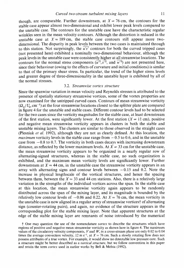
x (cm) FIGURE 21. Streamwise development of maximum derived turbulence parameters :

(a) (q2/Ui)maz; (b) (uJmaz. See figure 19 for key.

compared to those for the other cases. The peak ulWl for the untripped stable case starts off at a much lower level, but still higher than those for the tripped cases. However, beyond X = 95 cm, the peak levels for this ~ case are comparable to those for the other tripped cases. Not surprisingly, the peak u'w' levels for the three tripped cases start off relatively low and remain low, since no significant spatially stationary streamwise vorticity is generated in these cases. It is interesting to note that the u/wI level for the tripped unstable case shows a slow increase beyond X z 200 cm.

The streamwise evolution of (twice) the maximum turbulent kinetic energy, ?/ U,Z, (formed by summing the maximum spanwise-averaged normal stresses) is plotted in figure 21 (a). Downstream of X z 100 cm, all of the tripped and untripped data pairs exhibit good agreement. The stable and straight cases asymptote to approximately the same value of ?/U," of approximately 0.07. In contrast, the levels in the unstable cases, which consistently lie above the straight and stable curves, continue to increase monotonically. At the most downstream stations, the stationary streamwise vorticity is quite weak, even in the unstable case. The continued evolution of the turbulent kinetic energy is due to the destabilizing curvature, and it indicates that an asymptotic self-similar state is not established.

Figure 21 (b) is a plot of the streamwise evolution of the structure parameter formed


1 .2 , I 1

- 0.2 1.2

1 .0

0.8

0.6

0.4

0.2

0

- 0.2 -4 -2 0 2 4 -4 -2 0 2 4

17 17

U *

--8--- X = 11 cm -+-- X = 141 cm -e-- 33cm + 162cm --&- 44 cm -+-- 189 cm + 76 cm -+-- 221 cm * 95 cm --+I+-- 254 cm --+- 125cm

FIGURE 22. Mean streamwise velocity profiles in similarity coordinates for all streamwise locations : (a) untripped unstable case; (b) untripped stable case; (c) tripped unstable case; ( d ) tripped stable case.

by taking the ratio of the maximum Reynolds shear stress to the maximum turbulent kinetic energy as defined above. The structure parameter (often referred to as a,) is a measure of how efficient a turbulent flow is in producing Reynolds shear stress. Turbulent kinetic energy is extracted from the mean flow primarily by the interaction of the Reynolds shear stresses with the mean velocity gradients. Since Reynolds stress production is associated with the large-scale structures in the mixing layer, a,, reflects to what degree the large-scale structures increase correlated motions in Reynolds shear stress production. Note that the structure parameter for the tripped cases has its highest value at the first station, and decreases slightly further downstream. In contrast, the untripped cases approach the far-field values from considerably lower initial values. The straight layers (tripped and untripped) reach asymptotic values of about 0.16 in the far-field, as does the untripped stable case. The tripped stable case exhibits somewhat lower values, which appear to be evolving even at the farthest downstream stations. The tripped and untripped unstable case have levels higher than the stable and straight cases, and appear to be increasing in magnitude with streamwise distance. So the effects of curvature seem to be to accelerate the rate of production compared to that of in the unstable case, and vice versa for the stable case. The behaviour of the maximum Reynolds stresses suggests that the straight mixing layers have attained an asymptotic turbulent state by the last streamwise measuring station, while the curved mixing layers are still evolving owing to the effects of curvature. In general, the observed effects of curvature on the maximum Reynolds stresses, namely


0.05

0.04

u f 2 0.03 - -

Ui 0.02

0.01

0 0.05

0.04

2 2 0.03 -

u6 0.02

0.01

0 -4 -2 0 2 4 -4 -2 0 2 4

17 17 * X = 11 cm --O- X = 142cm -8- 33cm * 162cm --b 44cm --%- 189cm + 76cm --c 221 cm - 95 cm + 254cm - 125cm

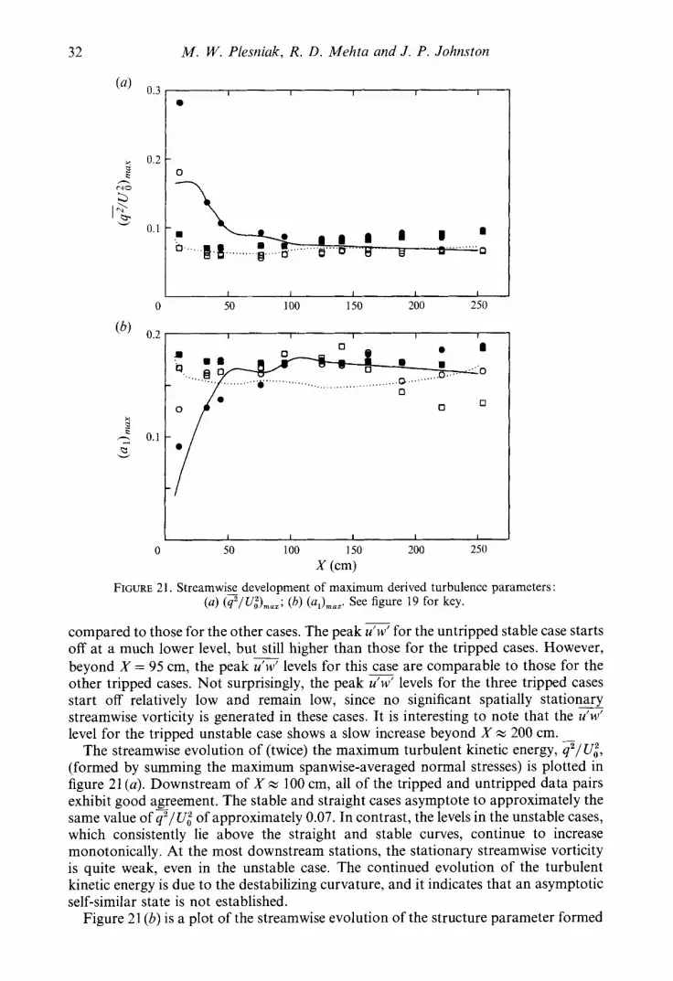
FIGURE 23. Streamwise normal stress (p/u;5) profiles in similarity coordinates for all streamwise locations : (a) untripped unstable case; (b) untripped stable case; (c) tripped unstable case; (d ) tripped stable case.

that destabilizing curvature leads to increased stress levels, whereas stabilizing curvature has a decreasing trend, are consistent with the previous observations of Margolis & Lumley (1965), Wyngaard (1967), Wyngaard et al. (1968), Castro & Bradshaw (1976), Gibson & Younis (1983), and Plesniak & Johnston (1989a, b).

3.4.3. Examination of proJile similarity In order to further examine the approach to self-similarity (or lack thereof),

spanwise-averaged profiles of mean velocity, Reynolds stresses, triple products and higher-order moments are plotted in similarity coordinates. Straight mixing-layer similarity profiles are omitted for the sake of brevity, but can be found in Bell & Mehta (1990).

Figure 22 shows profiles of the mean velocity (U*) for the untripped and tripped curved cases. Note that in all of these cases, excellent collapse is exhibited after the first measuring station. In the tripped cases, the effect of the wake is more apparent than in the untripped cases owing to the thicker boundary layers on the splitter plate. A collapse of this kind is not expected in the curved cases, since for the mixing layer to be self-similar, the quantity 6 / R which appears in the momentum equation, should remain constant. In these cases, the radius of curvature is held constant (test-section is formed by two nearly concentric circular arcs), while 6 increases with streamwise distance. Thus, &/a increases, and consequently the curvature ‘gets stronger’ with


0.05

0.04

7 2 0.03 - a 0.02

0.01

0

- G 0.02

0.01

0 -4 - 2 0 2 4 -4 -2 0 2

17 17 FIGURE 24. Cross-stream normal stress (v'"/ U i ) profiles in similarity coordinates for all streamwise locations: (a) untripped unstable case; (b) untripped stable case; (c) tripped unstable case; ( d ) tripped stable case. See figure 23 for key.

streamwise distance, but still remains relatively weak (< 3 Yo). Again, as has been found in straight mixing layers (Bell & Mehta 1990), the apparent collapse of mean velocity profiles is a poor indicator of self-similarity.

Profiles of the streamwise normal Reynolds stress (u'"/U,") are presented in figure 23. The profiles for the unstable cases clearly show higher maximum levels than those in the stable cases. In addition, the profile at the first station for the untripped unstable case exhibits a double-peaked distribution, probably caused by the orderly passage of spanwise vortices (Mehta et al. 1987), whereas that of the stable case only shows a single peak. Downstream of X = 33 cm, both unstable cases exhibit maximum values ranging from about 0.035 to 0.040. The profiles in the unstable cases also show a continuous evolution up to the last station, with the maximum level increasing monotonically with streamwise distance. In the untripped stable case, the profiles downstream of the first three stations show adequate collapse, with maximum levels ranging from 0.025 to 0.027. The tripped stable case also exhibits good collapse after the first station with a maximum level of about 0.025, but then decreases to a value of 0.023 at the last two or three stations.

The transverse normal Reynolds stresses (v,"/U,"), plotted in figure 24, show two main differences compared to the u'" results. There is a less satisfactory degree of collapse, in general, and the maximum levels among all four cases are more nearly equal, although those in the unstable cases are still slightly higher. In the untripped unstable case, downstream of the first four stations, the profiles show a peak value of about 0.023, with a moderately increasing trend exhibited at the last five stations. In the tripped unstable case, the maximum value of p/ U: increases monotonically with streamwise distance, and ranges from 0.020 to 0.025. It is interesting to note that the curves appear to group together in combinations of two or three. For example, the curves at X = 189 and 221 cm exhibit excellent collapse, as do those at X = 125, 141

36 M . W. Plesniak, R . D . Mehta and J . P. Johnston

0.05

0.04

wq 0.03 - - u; 0.02

0.01

0 0.05

I t

-2 0 2 4 -4 -2 0 2 4

77 17 FIGURE 25. Spanwise normal stress (p/ U,"), profiles in similarity coordinates for all streamwise locations: (a) untripped unstable case; (b) untripped stable case; (c) tripped unstable case; ( d ) tripped stable case. See figure 23 for key.

and 162 cm although with a different shape and maximum level. The untripped stable case exhibits values ranging from 0.018 to 0.020, while the corresponding tripped case has values in the range of 0.020 to 0.025.

The profiles of the spanwise normal Reynolds stress (w'2/ U,") are presented in figure 25. The profiles for the stable cases exhibit some degree of similarity while those for the unstable case are clearly changing, with a generally increasing trend (in peak levels) with streamwise distance in the tripped case. In addition, at the streamwise locations downstream of X = 11 cm, the overall peak levels are about 50 % higher for the unstable cases. In the stable cases, the maximum values range from about 0.017 to 0.020 while in the unstable cases they range from about 0.025 to 0.029.

Profiles of the primary Reynolds shear stress (u"/U,") are presented in figure 26. Except for the untripped stable case, which shows good collapse of the profiles downstream of X= 95 cm, the results for the other three cases clearly indicate that profile similarity has not been achieved. The tripped stable case shows a generally decreasing trend for the shear stress with the peak levels ranging from 0.012 to 0.007. On the other hand, both the unstable cases indicate an increasing trend with streamwise distance where the maximum primary shear stress values range from 0.0 14 to 0.017. With the exception of the untripped stable case, all of the mixing layers seem to be evolving throughout the test section, and the shear stress does not appear to attain an asymptotic value.

It is apparent from the profiles of the Reynolds stresses plotted in 'similarity' coordinates, that in almost all cases, the turbulence structure is still evolving right up to the end of the test section without any signs of reaching an equilibrium state. Therefore, in order to compare the effects of curvature at a representative streamwise location, the maximum values of the Reynolds stresses at X = 254 cm (the last station) are presented in table 5. Also included are the ratios of unstable to straight, stable to


0.025

0.020

0.015

- 0.010

0.005

0

- u )v/ G

- 0.005 GG

0.015

- 0.010

0.005

0

- ufv' u8

0.005 J I I -4 -2 0 2 4 -4 -2 0 2 4

77 77 FIGURE 26. Primary shear stress ( n / U , " ) profiles in similarity coordinates for all streamwise locations: (a) untripped unstable case; (b) untripped stable case; ( c ) tripped unstable case; (d ) tripped stable case. See figure 23 for key.

Untripped cases

Unstable to

Quantity Unstable Straight Stable straight u"/U," 0.041 0.030 0.028 1.38 B U ; 0.026 0.015 0.019 1.68 w'2/Ui 0.030 0.022 0.020 1.36 D U , " 0.096 0.067 0.067 1.44 u'u'/U," 0.018 0.011 0.011 1.68

Tripped cases

-

Stable Unstable to to

straight stable 0.94 1.47 1.26 1.33 0.90 1 S O 1 .oo 1.44 1.01 1.66

- u"/U," 0.040 0.033 0.027 1.22 0.82 1.49 B U , " 0.026 0.018 0.020 1.40 1.10 1.28 w"/U," 0.028 0.021 0.019 1.35 0.89 1.52 a U , " 0.094 0.072 0.065 1.30 0.91 1.43 u'v'/U," 0.017 0.012 0.008 1.43 0.71 2.01

TABLE 5. Reynolds stress maxima ratios at X = 254 cm

straight, and unstable to stable values for both the untripped and tripped cases. The unstable normal stress levels are about 1.5 times higher than the stable ones for both initial conditions. The ratio is somewhat lower for ?, mainly because the stable levels are comparable to the straight levels whereas and w'2 are lower. The untripped stable is also comparable to the untripped straight value, but since the unstable level is much higher, this gives an unstable to stable ratio of about 1.7. In contrast, for

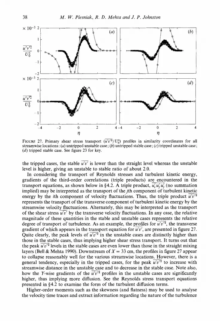
38 M . W. Plesniak. R. D. Mehta and J . P. Johnston

-4 -2 0 2 4 -4 -2 0 2 4

77 17 FIGURE 27. Primary shear stress transport ( m / U i ) profiles in similarity coordinates for all streamwise locations: (a) untripped unstable case; (b) untripped stable case; (c) tripped unstable case ; ( d ) tripped stable case. See figure 23 for key.

the tripped cases, the stable is lower than the straight level whereas the unstable level is higher, giving an unstable to stable ratio of about 2.0.

In considering the transport of Reynolds stresses and turbulent kinetic energy, gradients of the third-order correlations (triple products) are encountered in the transport equations, as shown below in $4.2. A triple product, u; uj uj’ (no summation implied) may be interpreted as the transport of the j th component of turbulent kinetic - energy by the ith component of velocity fluctuations. Thus, the triple product u‘v‘~ represents the transport of the transverse component of turbulent kinetic energy by the streamwise velocity fluctuations. Alternately, this may be interpreted as the transport of the shear stress by the transverse velocity fluctuations. In any case, the relative magnitude of these quantities in the stable and unstable cases represents ~ the relative degree of transport of turbulence. As an example, the profiles for U‘U‘’, the transverse gradient of which appears in the transport __ equation for a, are presented in figure 27. Quite clearly, the peak levels of u‘d2 in the unstable cases are distinctly higher than those in the ~ stable cases, thus implying higher shear stress transport. It turns out that the peak u’u’’ levels in the stable cases are even lower than those in the straight mixing layers (Bell & Mehta 1990). Downstream of X = 33 cm, the profiles in figure 27 appear to collapse reasonably well for the various streamwise locations. - However, there is a general tendency, especially in the tripped cases, for the peak u’u’’ to increase with streamwise distance in the unstable __ case and to decrease in the stable case. Note also, how the Y-wise gradients of the u’v’’ profiles in the unstable cases are significantly higher, thus implying more diffusion. See the Reynolds stress transport equations presented in $4.2 to examine the form of the turbulent diffusion terms.

Higher-order moments such as the skewness (and flatness) may be used to analyse the velocity time traces and extract information regarding the nature of the turbulence


-3 ' I -4 -2 0 2 4 -4 -2 0 2 4

17 17 FIGURE 28. Skewness (u-component) profiles in similarity coordinates for all streamwise locations : (a) untripped unstable case ; (b) untripped stable case; (c) tripped unstable case; (d) tripped stable case. See figure 23 for key.

in the flow. Skewness is the third moment of velocity and is a measure of the symmetry of the probability density function (PDF). The skewness profiles for the u-velocity component are compared in figure 28. It is observed that the skewness is close to zero in the free stream and at the centreline, thus indicating symmetric PDFs. The skewness attains positive values on the low-speed side and negative values on the high-speed side. Positive and negative peaks are observed between 171 = 1.0 and 1.5, with the peaks sharper in the unstable cases. The magnitudes of the extrema in the stable layers generally decrease with increasing streamwise distance to approximately 1 .O in the untripped case and 0.5 in the tripped case. The shape of the skewness profiles for the unstable layers is similar to that of the stable layers. However, the magnitude of the extrema is considerably larger, ranging from 1.5 to 2.0 in the tripped and untripped cases, respectively. The interpretation of these profiles for the u-component is that turbulence which emanates from the central, highly disturbed region of the mixing layer creates disturbances that propagate to the edges. The disturbances represent an impelling influence on the low-speed side and a retarding influence on the high-speed side. Hence, a positive skewness is observed on the low-speed side and a negative skewness on the high-speed side.

4. Further discussion 4.1. Three-dimensional structure

The primary effect of weak longitudinal curvature on two-stream mixing layers originating from laminar initial conditions is to affect the initial (near-field) decay rate of the secondary streamwise vortical structures. The role of curvature in creating the three-dimensionality observed in the initial regions of the untripped mixing layers appears to be weak or non-existent. In all three untripped cases, the initial levels of


(L?,),,, (see figure 6) are comparable (especially if the results of the curved cases are extrapolated from X = 11 cm back to X = 8 cm, as suggested above in $3.2). Thus, the present results indicate that curvature does not affect the initiation or production of mean streamwise vorticity (or three-dimensionality) in any of the cases investigated.

In the near-field regions of the untripped mixing layers (curved and straight), clusters of mean streamwise vorticity are present (see figure 4). However, at X= 11 cm, there are already differences between the stable and unstable cases in the levels and spanwise distribution of these structures. The curvature (which is applied at the origin of the mixing layer, X = 0 cm) seems to affect the development of the streamwise vorticity immediately, i.e. from the point at which the streamwise structures appear (at X % 5 cm based on the results of Bell & Mehta, 1992 for the straight case). In the straight case, where the effects of swapping high- and low-speed sides were investigated (Plesniak et al. 1992, 1993), no such differences in initial streamwise vorticity levels were observed. Thus, in the curved cases, these differences are attributable to the early effects of curvature and not to the change in initial conditions.

Therefore, in two-stream mixing layers, mild longitudinal curvature does not affect the genesis of streamwise vorticity, but influences its evolution, resulting in stronger streamwise vortices in the unstable case and weaker ones in the stable case, compared to the straight case. Consequently, the three-dimensionality is greatest for the unstable layer and weakest in the stable layer. Higher levels of Reynolds stresses accompany the greater three-dimensionality in the unstable case (see figure 3). These results are consistent with the earlier observations of Plesniak & Johnston (1989a, b).

The present results also suggest that mild curvature has no apparent effect on the mean three-dimensional structure of the tripped mixing layers, since no spatially stationary streamwise vorticity is present in any of these cases. It should be noted that, even though spatially stationary streamwise vortical structures are not observed in the tripped cases, the same mechanisms responsible for generating these structures in the untripped layers are also present in these cases. And indeed, numerical simulations of a mixing layer developing from turbulent velocity fields do show the presence of streamwise vortices, or ribs, in the early part of the development (Moser & Rogers 1992). The fact that these structures are not spatially stationary in the tripped layers is due to the turbulent initial conditions, which provide a variety of (time-varying) disturbances for amplification. Similar behaviour was reported by Bell & Mehta (1990) for straight mixing layers. However, in the curved (unstable) cases, there is the additional Taylor-Gortler instability mechanism which can potentially produce large- scale streamwise vortical structures. Although not observed here, strong curvature may have a greater effect, and may lead to the formation of streamwise vortices analogous to the Taylor-Gortler rollers observed in boundary layers on concave surfaces (cf. Barlow & Johnston 1988). Boundary layers are fundamentally different (structurally) to mixing layers in that there are no structures analogous to the Kelvin-Helmholtz spanwise rollers or relatively strong spatially stationary streamwise vortices present in boundary layers. Thus, the streamwise rollers can form, without competing with other dominant structures. In the mixing layer, the Kelvin-Helmholtz structures are always present, and the rib vortices are generated in the braid regions. The strength of the rib vortices should be dependent on that of the spanwise vortices, since the latter determines the amount of stretching in the braid region. The strength of the spanwise vortices is essentially determined by the mean shear aU/a Y which, in turn, is dependent upon the velocity difference across the mixing layer. As the velocity difference of the mixing layer is decreased, the Kelvin-Helmholtz spanwise vortices become weaker, and


this should result in weaker streamwise vortices. So, although the present study did not address the issue of structural dependence on the degree of curvature or on the mixing- layer properties, it is hypothesized here that Taylor-Gortler rollers may form in curved mixing layers when the ratio of the centrifugal to mean shear ‘forces’ exceeds a critical value. The following dimensionless parameter which expresses this ratio is proposed : ( f i / R ) / ( U,/d) where fi = :( V, + V,) is the average convection velocity. However, the critical value of this parameter cannot be prescribed without additional experiments in which the strength of curvature, velocity difference and velocity ratio are systematically varied.

There are some issues about the time-averaged measurement techniques employed in this study which should be addressed. First, structures with dimensions on the order of the cross-wire tip size (- 1 mm), or less, will obviously not be resolved in the measurements. Secondly, only spatially stationary streamwise vortical structures with long effective ‘lifetimes’ will be resolved. The secondary velocity (V and W ) field at a given streamwise location is obtained from two separate scans through the measurement grid, each typically taking about four hours to acquire. Therefore, for a structure to be identified in the mean streamwise vorticity contours, it must be spatially stationary and make a continuous contribution to the secondary velocities over the relatively long total data acquisition time. This type of contribution could come from a long continuous vortex or, as in the present case, from multiple (repetitive) streamwise vortical structures. The current model of the rib streamwise vortices is that they essentially reside in the braid regions connecting adjacent spanwise roll-ups, with their ‘phase’ locked so that each streamwise vortex makes similar (consistent) contributions to the secondary velocity measurement at a given point. For example, at X = 76 cm, the measurement of each secondary velocity is averaged over about 250 streamwise structures during the 3.33 s data acquisition time. It is, therefore, possible that some streamwise vortical structures which are either extremely small in cross-section, spatially variant or relatively short and isolated will be missed by the present measurement technique. In particular, just because the present technique does not detect any streamwise vortical structures, such as in the tripped cases, does not necessarily mean that no streamwise vorticity is generated, and that it is completely unaffected by curvature.

The limitations of the measurement technique lead to the possibility that the observed decay of mean streamwise vorticity with downstream distance may be due to a smearing caused by the meander of the structures about the detection point, rather than due to actual diffusion of vorticity. However, the balance of evidence suggests that the diffusion is real, rather than an artefact of meander. Some recent two-point correlation measurements by LeBoeuf & Mehta (1993) show that there is no measurable vortex meander, at least in the spanwise (2) direction. Correlation measurements made across the mixing layer in the cross-stream ( Y ) direction are not as easy to interpret. Since the rib vortices are inclined with respect to the streamwise direction (cf. Jimenez et al. 1985), a fixed probe will detect an apparent meander in the vertical direction at the local spanwise vortex passage frequency. This apparent meander is basically responsible for the non-circular cross-sectional shapes (elongated in the vertical direction) of the vorticity contours in figure 4. The implication of these results is that the streamwise vortical structures will not persist through to the far-field (self-similar) region, which is exactly what was observed in the temporal numerical simulations of Moser & Rogers (1992).

In order to investigate the measured effects of curvature on the decay of the mean

42 M . W. Plesniak, R. I). Mehta and J . P. Johnston

(4 5

h

v f j 0 x

-5 -15 - 10 -5 0 5 10 15

Contour Value 1 ---0.006 2 - - - -0.004 3 - - - - - -0.002 4 ......... - 0.001 5 - 0.001 6 - - 0.002 7 0.004 8 - - - - - 0.006

Contour Value 1 - - -0.005 2 - - - -0.004 3 - - - - - -0.003 4 . . ' ' " -0.002 5 - -0.001 6 - - 0.001 7 0.002 8 - - - - - 0.003

-5 1 I I I I I I -15 -10 -5 0 5 10 15

(cm) - _ FIGURE 29. Normal stress anisotropy ( ( U ' ~ - - W ' ~ ) / U ~ ) contours at X = 76 cm: (a) untripped

unstable case; (b) untripped stable case.

_ _ streamwise vorticity, the anisotropy term (0''- w ' ~ ) was examined. Bell & Mehta (1992) showed, by means of a relatively simple order-of-magnitude analysis on the mean streamwise vorticity transport - - equation, that the only significant production (or maintenance) term is az//a Y ~ Z ( U ' ~ - d2). In the idealized case, the streamwise vorticity should decay as 1/X2 if this term is negligible. It is not feasible - - to obtain the second derivative of the anisotropy parameter, but the contours of ( ~ P - W ' ~ ) for the two untripped curved cases at X = 76 cm are presented in figure 29. Note that saddle points oriented at 4.5" to the Y- and Z-axes correspond to regions - - of high production of streamwise vorticity (local maxima). Quite clearly, the (v" - w") distribution for the unstable case (figure 29a) exhibits about five such saddle points across the measured span and centred around the mixing-layer centreline, whereas these data for the stable case (figure 29b) do not appear to have any saddle points. This is at least part of the reason why the vorticity in the unstable case decays at a slower rate.

The behaviour of the streamwise vortex circulation and vortex spacing for the untripped curved cases is, in general, very similar to that of the untripped straight case. All cases exhibit approximately constant circulation with temporary increases and decreases. The increases in circulation (per vortex) occur approximately at locations where the vortex spacing also increases. As discussed above in 53.2, these are the locations where amalgamation of like-signed streamwise vortices could be taking place. The similarities in behaviour are not too surprising since, once the streamwise vorticity is formed, its subsequent evolution is not expected to be curvature dependent, although the mean vorticity decay is affected. The differences in vortex spacing between the stable and unstable cases are generally comparable to those observed for the two untripped straight cases (Plesniak et al. 1993). However, the differences in circulation levels seem to be real, although the mechanism responsible for them is not obvious.

The increased mean three-dimensionality, caused by the presence of stationary


sireamwise vortical structures, shows up clearly in the mean velocity and Reynolds stress distributions, in the form of large spanwise distortions. This is due to a direct effect of the vortical structures on the momentum and Reynolds stress transport, such that a peak is produced in the region of upwash, and a valley in that of downwash. These periodic wrinkles appear, with a wavelength that scales approximately with twice the local mixing-layer thickness. Since SZ, is strongest at a given station for the unstable layer, larger spanwise variations in mean velocity and Reynolds stresses are observed, implying more transport of momentum and Reynolds stresses in the cross-plane. Production of Reynolds stresses is also affected, since the streamwise mean velocity gradients, (e.g. aU/c?Y and aU/aZ) are modified, and additional spatial gradients of the secondary velocities are generated by the presence of the streamwise vorticity. For example, the spanwise variation in (?U/L?Y is responsible for the local peaks observed in the contours (figure 3), the dominant production term being v/"aU/c?Y. The three-dimensional Reynolds stress transport equations are presented below in 54.2, and the role of curvature in the production and transport of turbulence is discussed more

4.2. Streamwise evolution It has been shown that the growth rate in the linear region is affected by the initial conditions, namely the sate (laminar or turbulent) of the initial boundary layers (Bell & Mehta 1990). Bell & Mehta found that the straight mixing layer originating from turbulent initial boundary layers did not contain organized streamwise vorticity and had a growth rate of 0.019, approximately 20 % lower than the case with laminar initial boundary layers. Most of the growth in a mixing layer is achieved through engulfment of potential fluid during the pairing of adjacent spanwise vortices, and also through entrainment by these structures themselves. The presence of organized streamwise vorticity, riding over the spanwise vortices, adds to the entrainment process, resulting in a higher net growth rate. Of course, the state of the initial boundary layers may also affect the structure and dynamics of the spanwise vortices themselves, thereby affecting the primary entrainment, as discussed by Bell & Mehta (1993). In fact, the spectral measurements at X = 11 cm (figure 9) do show significant differences with the fundamental peak (owing to the Kelvin-Helmholtz roll-up) only apparent in the untripped case.

In the present study, it was found that both curvature and the state of the initial boundary layers affect the growth rate of the mixing layer in the region downstream of X = 76 cm. The effect of curvature is to enhance the growth rate of the unstable layer with respect to the straight and stable layers, for both initial conditions. In addition, when the initial boundary layers are untripped, and stationary streamwise vortices are observed, the growth rate is highest for the unstable case. Additional entrainment due to the relatively strong streamwise vortices can enhance the growth rate for the untripped unstable case, as discussed above. In contrast, the growth rate (and mixing-layer thickness) in the stable case seems unaffected by curvature and state of the initial boundary layers. For laminar and turbulent initial conditions, the growth rate of the stable layer is almost exactly the same as that of the tripped straight layer. Thus, it must be concluded that the streamwise vorticity in the untripped stable case decays to such a low level so quickly that it does not influence the far-field development of the mixing layer.

The increased stress levels in the unstable cases may be partly attributable to 'extra' production through terms in the Reynolds stress transport equations which are activated by the angular momentum instability. The rate of strain ratio, S =

fully.

44 M . W. Plesniak, R. D. Mehta and J . P. Johnston (U/R) / (aU/a Y ) = - (aV/U)/(aU/c?Y), may be approximated as S J R . Since S,,, increases with downstream distance and R is constant, the ratio increases monotonically with streamwise distance. In the untripped cases, this parameter (measured from X = 11 cm to X = 254 cm) ranges from 0.003 to 0.035 in the stable case, and -0.002 to -0.048 in the unstable case. For the tripped cases, the values in the stable case range from 0.003 to 0.036, and from -0.0035 to -0.043 in the unstable case. Therefore, the effects of curvature are expected to become more pronounced with increasing streamwise distance.

The effects of streamline curvature on the production of turbulent stresses can manifest themselves in two ways: (i) explicitly through terms due to the extra rates of strain, and (ii) implicitly through changes in the turbulence structure which can enhance or suppress turbulence production, often referred to as ‘ higher-order effects ’. It is well known that the explicit terms do not account for all of the enhancement or suppression which is measured in flows with streamline curvature (Bradshaw 1973). The transport equations for the Reynolds stresses and turbulent kinetic energy presented below are based on the ‘fairly thin shear layer’ approximation (Bradshaw 1973), but additionally they are three-dimensional since terms involving mean spanwise velocity ( W ) , spanwise gradients (a/aZ), and the secondary Reynolds shear stresses (m and m) are retained. The ‘fairly thin shear layer’ approximation is valid for shear layers in which the ratio of the extra rates of strain (due to streamline curvature) to the primary strain, (aV/aX)/(aU/aY), is less than 0.1.

+PD+PS+ VD+D,

+ PD + PS+ VD + D,


+ PD + VD + D (no pressure strain term),

_ _ - u’U’2 - u‘3 a -

-- (u’u’w’) --(&)’)- 1 +- -(U’U’2)-2 ( 3:Y- R az 2 - ax

+PD+PS+VD+D,

D -

a - -- (u’2w’) - 1 + - - (U’V’W‘) - - (u‘w’2) ax a - ( aiil- az +PD+PS+VD+D, (6)

where PD = pressure diffusion, PS = pressure-strain correlations, V D = viscous diffusion and D = viscous dissipation.

In (1)-(6), the terms on the first line on the right-hand side represent production or generation, those on the second line represent production arising from mean flow three-dimensionality, and those on the third line represent turbulence transport by velocity fluctuations, or turbulent diffusion. For the sake of brevity, the terms on the fourth line are represented symbolically. The double underlined terms in (l), (2) and ( 5 ) are not true production terms, but represent the effects of the rotation of the coordinate axes (Bradshaw 1973). The transport equation for the turbulent kinetic energy (equation (4)), which is invariant under coordinate rotation, does not contain any ‘false’ production terms. In general, the explicit effects of curvature are expected to be reflected in the ‘extra’ production terms (first line), while the effects of mean flow three-dimensionality due to stationary streamwise vortices (in the untripped cases) are expected to activate the terms on the second line.

For both the stable and unstable mixing layers, the coordinates are chosen such that aU/iY < 0, and consequently u1zi’> 0. For the stable case, U / R < 0 and S = (U/R)/(BU/aY) > 0 ; whereas for the unstable case U/R > 0 and S < 0. Note that since Y 4 R, the terms with the coefficient (1 + ( Y / R ) ) = ((R+ Y ) / R ) z 1 are independent of the sign of Y or R and will contribute positively to production when aU/aY < 0. The dominant ‘extra’ production term arising explicitly from curvature in the u/2 equation is --n (- U/R) . When S > 0 (stabilizing curvature), the additional term suppresses


the production of p. The opposite is true for S < 0 (destabilising curvature), where the extra term enhances the production of p. Inspection of (2) reveals that since Vand its gradients are small, there are no significant additional production terms in the transport equation for 3 due to curvature, and the term arising from the mean flow three-dimensionality is also small. The untripped unstable v” in the near field is probably higher because of the contribution of the terms involving a V/a Y and aV/aZ. These terms are attributable to the strong streamwise vorticity present in the near fields of the untripped layers. However, in the far field, the streamwise vorticity has decayed substantially, making these terms insignificant, and the tripped and untripped values of collapse and are close to the stable layer levels. The production terms in the transport equation for p arise solely from mean flow three-dimensionality. In tho near - field, where strong streamwise vorticity is present, these terms lead to production of w”, but further downstream these terms are expected to have little effect. Thus, in the far field where the mean flow is quasi-two-dimensional, streamline curvature should have little effect on 3 and p. This is reflected in the data, with little change in the magnitude of ;;T” from case to case (figure 24). The slight changes in p (figure 25) between cases must be attributed to ‘higher-order effects’ or redistribution among the components. Among all of the Reynolds normal stresses, the differences in p between the stable and unstable (both tripped and untripped) are the greatest (figure 23). These differences are attributable in part to the production term given above, but also to the additional production due __ to shear stresses multiplied by spanwise gradients of the mean velocity given by -u’w’(aU/aZ) which is expected to be significant primarily in the near field of the unstable untripped case, where the streamwise vortices cause the wrinkles in U (figure 2) and generate substantial levels of the secondary shear stress m. - Note also that the production term in the transport equation for m, i.e. - w’2((aU/i3Z), contributes to the generation of the secondary shear stress due to spanwise variations in U.

An analysis of the dominant production terms in the primary Reynolds shear stress (27) transport equation,

indicates that the extra term, -p( - U/R) , enhances production for S < 0, and suppresses - production for S > 0. Other terms such as -u‘w‘(aV/aZ) and -u’w’ (aU/aZ) are not expected to contribute significantly in the far field, since the quantities uIw/ and i3Ula.Z are multiplied by the small quantities aV/aZ and m. However, the streamwise vorticity present most strongly in the untripped unstable case causes the levels of u121’ to be somewhat higher than in the corresponding tripped case.

So, although not all of the observed changes of Reynolds stress levels in the curved cases are explained by the transport equations, the trends exhibited are consistent. The fact that there are some higher-order effects, as for example, on p, which are not accounted for in the transport equations is what makes the computation of such flows difficult. Examination of the velocity spectra further elucidates the turbulence structure.

The spectral data show some interesting trends in terms of the effects of curvature. The streamwise development results for the stable cases (figures 15 and 17) show that the spectral distributions continue to change with streamwise distance right up to the end of the measurement domain. This is not too surprising, since some of the Reynolds stresses, such as W, also show a changing trend as the curvature parameter 6 / R increases with streamwise distance. However, in the unstable case, where the Reynolds stresses indicate an even stronger changing trend in the far-field region (X > 100 cm),

Curaed two-stream turbulent mixing layers 47

the spectral distributions (figures 14 and 16) indicate a reasonable collapse at the higher-frequency end ( f > 100 Hz). The implication of these results is that while the fine-scale structures in the unstable cases have reached an equilibrium, the stable cases continue to reorganize such that the energy in the fine-scale structures decreases, hence leading to slowly decreasing stress levels. The effect of the stabilizing curvature appears to be to reorganize the spanwise vortex rollers, such that the mixing layer is dominated by these larger scales, and as discussed above, their passage, therefore, produces a stronger peak (at f z 20-50 Hz) in the downstream spectra (figure 11). On the other hand, destabilizing curvature seems to mainly affect the larger scales, with the finer scales exhibiting an asymptotic state in the downstream region. Therefore, the increasing energy in the larger scales (low-frequency end) leads to the increasing Reynolds stress levels in the unstable cases. However, a reorganization of the spanwise vortex rollers, as in the stable case, does not appear to occur, and the unstable layer at the last downstream station (X = 254 cm) is probably more three-dimensional than the stable layer. In any case, the results in figure 11 clearly show that the spectral structure of the curved mixing layers in the far-field region is independent of the initial conditions, but is dependent on the sense of curvature (stabilizing or destabilizing).

5. Conclusions A study of the effects of stabilizing and destabilizing streamwise curvature on the

three-dimensional structure and streamwise development of a two-stream mixing layer with tripped and untripped initial boundary layers has been completed. For the untripped cases, the mean streamwise vorticity results show that the main effect of the destabilizing curvature is to retard the decay of the streamwise vorticity generated by the amplification of small incoming disturbances. This results in stronger mean streamwise vorticity in the unstable case at a given streamwise location. The streamwise vorticity produces significant spanwise variations in the mean velocity and Reynolds stress distributions. In the near field, the mean streamwise vorticity also affects the spanwise spectral content of the mixing layer. The effect of the stabilizing curvature, on the other hand, is to suppress the three-dimensionality by increasing the rate of decay of the streamwise vorticity. Therefore, the spanwise variations in mean velocity and Reynolds stress distributions are much smaller in this case. The streamwise vortex spacing generally increases in a stepwise fashion, with the jumps coinciding approximately with local increases in circulation. The overall circulation for a given case remains more or less constant, although the levels for the unstable case are generally higher than those for the straight case, while those for the stable case are lower. Near-field spectral data show that stabilizing curvature also alters the details of the spanwise (Kelvin-Helmholtz) vortices.

Spatially stationary streamwise vorticity was not generated in either mixing layer developing from tripped initial boundary layers. The effects of curvature on the mean three-dimensional structure of the layers were, therefore, not as obvious as in the untripped cases. No large-scale (spatially stationary) streamwise vorticity, such as Taylor-Gortler rollers observed in concave boundary layers, was generated by the destabilizing curvature in the tripped cases, but as noted earlier, small-scale or non- stationary streamwise vortical structures may be present but not detected. However, it was noted that the curvature was relatively weak in the present study, and a dimensionless parameter representing the ratio of centrifugal to mean shear forces was proposed in $4.1. It is hypothesized that Taylor-Gortler rollers may form when a critical value of this parameter is exceeded.

48 M . W. Plesniak, R. D. Mehta and J . P . Johnston

For the untripped initial conditions, the main effects of curvature are to increase the asymptotic growth rate of the unstable case and to decrease that of the stable case, compared to that of the straight case. A part of the increase in the unstable case is attributed to the presence of stronger stationary streamwise vortices, which would result in more entrainment. The peak Reynolds stresses are correspondingly affected - those for the unstable case are significantly higher than those for the straight case, while those for the stable case are comparable, or slightly lower. The main effect of tripping the boundary layers is to reduce the growth rate for the unstable case, although it is still higher than those for the stable and straight cases, which are comparable. The peak Reynolds stresses in the far field were not affected significantly by the tripping for both curved cases. Some of the peak Reynolds stress data clearly indicate that the levels continue to change right up to the end of the measurement domain. This is not too surprising, since the curvature is applied continuously and 6 /R increases with downstream distance. A part of the increase in Reynolds stresses is attributable to extra production through terms activated by the angular momentum instability. The velocity spectral data further confirm that the turbulence structure of the stable and unstable cases is different in the far-field region.

The present results clearly show that even very mild streamwise curvature ( 6 / R < 3 %) has profound and strong effects on the mixing-layer structure and streamwise development. Furthermore, the effects appear to manifest themselves as soon as the curvature is applied. The structure of the curved mixing layer in practice is, therefore, likely to be extremely complex, with its modelling posing an unenviable task.

This research was supported by The National Science Foundation Grant NSF-CTS- 88-1 5670 and NASA Grant NCC-2-55 from the Fluid Mechanics Laboratory (FML), NASA Ames Research Center and was conducted in the FML. We are grateful to Mr David A. Briggs, Stanford University for help with some of the data acquisition and reduction, and to Dr James H. Bell, NASA Ames Research Center for many useful discussions.

R E F E R E N C E S BARLOW, R. S. & JOHNSTON, J. P. 1988 Structure of a turbulent boundary layer on a concave

BELL, J. H. & MEHTA, R. D. 1 9 8 9 ~ Three-dimensional structure of plane mixing layers. JZAA Rep.

BELL, J. J. & MEHTA, R. D. 19896 Design and calibration of the mixing layer wind tunnel. JZAA

BELL, J. H. & MEHTA, R. D. 1990 Development of a two-stream mixing layer with tripped and

BELL, J. H. & MEHTA, R. D. I992 Measurements of the streamwise vortical structures in a plane

BELL, J. H. & MEHTA, R. D. 1993 Effects of imposed spanwise perturbations on plane mixing layer

BELL, J. H., PLESNIAK, M. W. & MEHTA, R. D. 1992 Spanwise averaging of plane mixing layer

BERNAL, L. P. & ROSHKO, A. 1986 Streamwise vortex structure in plane mixing layers. J. FluidMech.

BIRCH, S . F. & EGGERS, J. M. 1973 A critical review of the experimental data for developed free turbulent shear layers. NASA SP-321.

BRADSHAW, P. 1973 Effects of streamline curvature on turbulent flow. AGARDogruph 169. BROWAND, F. K. & LATIGO, B. 0. 1979 Growth of the two-dimensional mixing layer from a

surface. J . Fluid Mech. 191, 137-176.

TR-90, Dept of Aeronautics and Astronautics, Stanford University.

Rep. TR-89, Dept of Aeronautics and Astronautics, Stanford University.

untripped boundary layers. AZAA J . 28, 2034-2042.

mixing layer. J . Fluid Mech. 239, 213-248.

structure. J . Fluid Mech. 257, 33-63.

properties. AZAA J . 30 (3), 835-837.

170, 499-525.

turbulent and nonturbulent boundary layer. Phys. Fluids 22, 101 1-1019.


BROWAND, F. K. & TROUTT, T. R. 1985 The turbulent mixing layer: geometry of large vortices. J .

BROWN, G. L. & ROSHKO, A. 1974 On density effects and large structure in turbulent mixing layers,

CASTRO, I. P. & BRADSHAW, P. 1976 The turbulence structure of a highly curved mixing layer. J.

DZIOMBA, B. & FIEDLER, H. E. 1985 Effect of initial conditions on two-dimensional free shear layers.

GIBSON, M. M. & RODI, W. 1981 A Reynolds-stress closure model of turbulence applied to the

GIBSON, M. M. & YOUNIS, B. A. 1983 Turbulence measurements in a developing mixing layer with

GILLIS, J. C. & JOHNSTON, J. P. 1983 Turbulent boundary layer flow and structure on a convex wall

Ho, C.-M. & HUERRE, P. 1984 Perturbed free shear layers. Ann. Rec. Fluid Mech. 16, 365424. HOFFMANN, P. H., MUCK, K. C. & BRADSHAW, P. 1985 The effect of concave surface curvature on

HUANG, L.-S. & Ho, C.-M. 1990 Small-scale transition in a plane mixing layer. J. Fluid Mech. 210,

HUSSAIN, A. K. M. F. & ZEDAN, M. F. 1978 Effects of the initial condition on the axisymmetric free

JIMENEZ, J. 1983 A spanwise structure in the plane mixing layer. J. Fluid Mech. 132, 319-326. JIMENEZ, J. 1988 Linear stability of a non-symmetric, inviscid, Kgrman street of small uniform

vortices. J. Fluid Mech. 189, 337-348. JIMENEZ, J., COGOLLOS, M. & BERNAL, L. P. 1985 A perspective view of the plane mixing layer. J.

Fluid Mech. 152, 125-143. JOHNSON, P. L. & JOHNSTON, J. P. 1989 The effects of grid-generated turbulence on flat and concave

turbulent boundary layers. Rep. MD-53, Thermosciences Division, Dept of Mechanical Engineering, Stanford University.

KONRAD, J. H. 1976 An experimental investigation of mixing in two-dimensional turbulent shear flows with applications to diffusion-limited chemical reactions. Project SQUID Tech. Rep. CIT- 8-PU; and PhD Thesis, California Institute of Technology, 1977.

LASHERAS, J. C. & CHOI, H. 1988 Three-dimensional instability of a plane free shear layer: an experimental study of the formation and evolution of streamwise vortices. J. Fluid Mech. 189,

LASHERAS, J. C., CHOI, H. & MAXWORTHY, T. 1986 On the origin and evolution of streamwise vortical structures in a plane, free shear layer. J. Fluid Mech. 172, 231-258.

LEBOEUF, R. L. & MEHTA, R. D. 1993 Streamwise vortex meander in a plane mixing layer. Phys. Fluids A 5, 1983-1991.

MARGOLIS, D. P. & LUMLEY, J. L. 1965 Curved turbulent mixing layer. Phys. Fluids 8, 1775-1784. MEHTA, R. D. 1991 Effect of velocity ratio on plane mixing layer development: influence of the

splitter plate wake. Esps Fluids 10 (4), 194204. MEHTA, R. D., INOUE, O., KING, L. S. & BELL, J. H. 1987 Comparison of experimental and

computational techniques for plane mixing layers. Phys. Fluids 30 (7), 20542062. MEHTA, R. D. & WESTPHAL, R. V. 1986 Near-field turbulence properties of single- and two-stream

plane mixing layers. Exps Fluids 4, 257-266. MOSER, R. D. & ROGERS, M. M. 1992 Coherent structures in a simulated turbulent mixing layer.

Presented at the IUTAM Symposium on Eddy Structure Identification in Free Turbulent Shear Flows, Oct. 12-14, Poitiers, France.

MUCK, K. C., HOFFMANN, P. H. & BRADSHAW, P. 1985 The effect of convex surface curvature on turbulent boundary layers. J. Fluid Mech. 161, 347-369.

OSTER, D., WYGNANSKI, I. J. & FIEDLER, H. E. 1977 Some preliminary observations on the effect of initial conditions on the structure of the two-dimensional turbulent mixing layer. In Turbulence in Internal Flows (ed. S. N. B. Murthy), pp. 67-87. Hemisphere, Washington, DC.

Fluid Mech. 158, 489-509.

J . Fluid Mech. 64, 775-8 16.

Fluid Mech. 73, 265-304.

J . Fluid Mech. 152, 419442.

calculation of a highly curved mixing layer. J. Fluid Mech. 103, 161-182.

mild destabilizing curvature. Esps Fluids 1, 23-30.

and its redevelopment on a flat wall. J. Fluid Mech. 135, 123-153.

turbulent boundary layers. J. Fluid Mech. 161, 371403.

47 5-500.

shear layer: effects of the initial momentum thickness. Phys. Fluids 21, 1100-1 112.

53-86.

50

PATEL, R. P. 1978 Effects of stream turbulence on free shear flows. Aero. Q. 29, 3343. PLESNIAK, M. W. & JOHNSTON, J. P. 1989a Reynolds stress evolution in curved two-stream mixing

layers. Seventh Symposium on Turbulent Shear Flows, Stanford University, August 21-23, 1989. In Turbulent Shear Flows 7, pp. 239-252. Springer, 1991.

PLESNIAK, M. W. & JOHNSTON, J. P. 19893 The effects of longitudinal curvature on turbulent two- stream mixing layers. Rep. MD-54, Thermosciences Division, Dept of Mechanical Engineering, Stanford University.

PLESNIAK, M. W., BELL, J. H. & MEHTA, R. D. 1992 Sensitivity of the structure of untripped mixing layers to small changes in initial conditions. JZAA Rep. TR-107, Dept of Aeronautics and Astronautics, Stanford University.

PLESNIAK, M. W., BELL, J. H. & MEHTA, R. D. 1993 Effects of small changes in initial conditions on mixing layer three-dimensionality. Exps Fluids 14 (4), 28G288.

RODI, W. 1975 A review of experimental data of uniform density free turbulent boundary layers. In Studies in Convection (ed. B. E. Launder), 1, 79-165. Academic.

ROGERS, M. M. & MOSER, R. D. 1993 Spanwise scale selection in plane mixing layers. J. Fluid Mech.

SMITS, A. J. & WOOD, D. H. 1985 The response of turbulent boundary layers to sudden perturbations. Ann. Rev. Fluid Mech. 17, 321-358.

TOWNSEND, A. A. 1976 Structure of Turbulent Shear Flow, pp. 188-230. Cambridge University Press.

WANG, C. 1984 The effects of curvature on turbulent mixing layers. PhD thesis, GALCIT, California Institute of Technology.

WOOD, D. H. & BRADSHAW, P. 1984 A turbulent mixing layer constrained by a solid surface. Part 2. Measurements in the wall-bounded flow. J. Fluid Mech. 139, 347-361.

WYNGAARD, J. C. 1967 An experimental investigation of the small-scale structure of turbulence in a curved mixing layer. PhD thesis, Pennsylvania State University.

WYNGAARD, J. C., TENNEKES, H., LUMLEY, J. L. & MARGOLIS, D. P. 1968 Structure of turbulence in a curved mixing layer. Phys. FZuids 11 (6) , 1251-1253.

M . W. Plesniak, R. D. Mehta and J. P. Johnston

247, 321-337.

Documents

Curved two-stream turbulent mixing layers: three-dimensional structure and streamwise evolution