Embed Size (px)
Citation preview
HAL Id: tel-01172202https://tel.archives-ouvertes.fr/tel-01172202
Submitted on 7 Jul 2015
HAL is a multi-disciplinary open accessarchive for the deposit and dissemination of sci-entific research documents, whether they are pub-lished or not. The documents may come fromteaching and research institutions in France orabroad, or from public or private research centers.
L’archive ouverte pluridisciplinaire HAL, estdestinée au dépôt et à la diffusion de documentsscientifiques de niveau recherche, publiés ou non,émanant des établissements d’enseignement et derecherche français ou étrangers, des laboratoirespublics ou privés.
Strongly correlated photons in arrays of nonlinearcavities
Alexandre Le Boité
To cite this version:Alexandre Le Boité. Strongly correlated photons in arrays of nonlinear cavities. Quantum Physics[quant-ph]. Université Paris Diderot - Paris 7, 2015. English. tel-01172202
Université Paris Diderot-Paris 7Sorbonne Paris Cité
Ecole doctorale: Physique Ile-de-France
Laboratoire Matériaux et Phénomènes Quantiques
DOCTORAT
Physique
Alexandre Le Boité
Strongly correlated photons in arrays ofnonlinear cavities
Photons fortement corrélés dans des réseaux decavités non-linéaires
Thèse dirigée par Cristiano Ciuti et Giuliano Orso
Soutenue le 06 mai 2015
JURY
M. Johann BLATTER RapporteurM. Cristiano CIUTI Directeur de thèseM. Rosario FAZIO RapporteurM. Markus HOLZMANN ExaminateurM. Giuliano ORSO Co-directeur de thèseM. Olivier PARCOLLET Examinateur

Remerciements
Je voudrais tout d’abord remercier le directeur du laboratoire, Carlo Sirtori, pour m’avoiraccueilli à MPQ pendant cette thèse.
Je suis reconnaissant à Gianni Blatter et Rosario Fazio d’avoir accepté d’être rapporteursde ma thèse. Leur mérite est d’autant plus grand qu’ils sont venus de loin pour assister à masoutenance. Un grand merci également à Markus Holzmann et Olivier Parcollet, mes autresexaminateurs, pour l’intérêt qu’ils ont porté à mon travail.
Je souhaite bien sûr remercier ici Cristiano Ciuti. De ses nombreuses qualités scien-tifiques, je retiendrai tout particulièrement son inventivité débordante et sa grande culture.On l’aura compris, ces qualités assurent la réussite du chercheur. Quand elles se doublentde qualités humaines indéniables, elles en font également un excellent encadrant : son sensde l’humour et son enthousiasme indéfectible m’auront été tout aussi précieux pendant cestrois années et demie.
J’ai également eu la chance d’être encadré par un second chercheur exceptionnel, GiulianoOrso. Qu’il en soit ici remercié. J’ai beaucoup appris de sa manière calme et assuréed’aborder les problèmes physiques, bien loin de l’image mythologique du théoricien illuminé etdéconnecté du monde réel. Je garde un souvenir ému de nos nombreuses conversations extra-scientifiques, toujours riches en anecdotes, contées avec un talent certain de la narration.Mon seul regret sera sans doute ne pas avoir rencontré les trois petits protagonistes dont ilétait souvent question...
Le dynamisme de l’équipe théorie doit aussi beaucoup à ses autres membres, que j’ai eugrand plaisir à côtoyer. Je voudrais remercier tout particulièrement ceux avec qui j’ai eula chance de collaborer directement, à commencer par Alexandre, qui s’est lancé avec moidans la “méthode du corner” pendant la dernière partie de ma thèse. Outre notre travail encommun, partager nos idées sur l’enseignement de la physique (ou le choix des meilleuresséries...) a toujours été un plaisir. Je dois même avouer que son humour, pourtant si par-ticulier, m’a beaucoup manqué après son départ. Merci également à Stefano, qui nous a
i
ii
rejoint par la suite et dont la participation cruciale au projet m’a beaucoup apporté. Merci àFlorent, dont le coup de pouce sur la fin fut salutaire et qui, j’en suis certain, fera une excel-lente thèse. Je n’oublie pas les autres membres de l’équipe, tout particulièrement Luc, Juanet notre escapade à Batimore, et Loïc, le théoricien stoïcien de la bande. Merci aussi aux“anciens”, Simon, David, Pierre et Motoaki, pour leur accueil à mes débuts dans le labora-toire. Merci aux autres thésards et post-docs du groupe, arrivés plus récemment, Jared, Mizio,Wim, Nicola et Riccardo. Merci à Mickael pour nos conversations cinémato-philosophiquesqui j’espère ne s’arrêteront pas là. Merci à Tom, Giulia, Andreas et aux autres membresde la composante info quantique. Merci à Indranil et Édouard pour nos échanges toujoursenrichissants.
Je remercie également nos collaborateurs du projet Quandyde pour nos nombreuses dis-cussions stimulantes: merci à Jacqueline Bloch, Alberto Amo et leur équipe du LPN, augroupe d’Alberto Bramati au LKB et à celui de Guillaume Malpuech à l’Institut Pascal.
S’il est vrai que la recherche est souvent un travail solitaire, les doctorants ne sont que trèsrarement seuls dans leur bureau. Je souhaite ici remercier tous les occupants du “thésarium”645B, dont j’ai déjà cité quelques-uns, pour tous les moments mémorables passés ensemble.Je n’oublierai pas nos nombreuses soirées “wine and cheese” sur la terrasse (ou plutôt chipset bière...), le mölkky entre midi et deux, l’abonnement Bein sport pour la coupe du monde etle séminaire thésard et son petit déj. Merci, donc, à Jo Buhot pour sa bonne humeur et sonsens de l’humour, à Philippe pour les raclettes “norvégiennes”, à Constance et Charlotte, mesanciennes voisines de “l’îlot central”, pour leur présence réconfortante. Merci à Siham poursa théorie des beaux gosses, à Pierre pour les BN fraise et le jus d’orange à l’eau chaude.Merci à Hélène pour sa gentillesse et sa générosité à toute épreuve. Merci, à JB, thésarddébonnaire, à Romain, Elisa, Bastien, Roméo, Pauline, Ludivine.
Merci aux permanents de l’équipe SQUAP, Alain, Marie-Aude, Max et Yann, avec quij’ai eu l’occasion de partager de nombreux déjeuners, goûters et pauses thé.
Je voudrais également remercier l’équipe administrative du laboratoire, en particulierAnne et Jocelyne, pour leur efficacité et leur gentillesse.
Merci à Irène, Chloé, Thierry, Doan, Ammara et Benjamin pour tous les momentspartagés. Merci à Colin et Dominique d’être venu me voir le jour J.
Je souhaite remercier à nouveau ma tante, Jacqueline Bloch. Son soutien et ses conseilséclairés remontent à mes tous premiers enthousiasmes pour la physique quantique et m’ont
Strongly Correlated Photons in Arrays of Nonlinear Cavities iii
accompagné jusqu’à aujourd’hui.Je voudrais remercier également mes grands-mères Adi et Myriem pour leur présence
chaleureuse le jour de ma soutenance.Merci aux Fischer, Mattout et Horowitz pour leurs encouragements et leur intérêt pour
mes travaux.
Un immense merci à mes parents et à mon frère pour leur soutien de tous les instants.Vous savoir à mes côtés m’a été pendant ces années, et me sera toujours, très précieux. Cettethèse vous doit beaucoup.
Je n’oublie pas Célia et ses nombreux conseils pratiques très appréciés.Merci à également à la famille Chan-Lang, Solène pour nos longues discussions diverses
et variées et pour ses macarons désormais célèbres, Sion pour ses conseils avisés sur maprésentation et ses leçons sur la théorie quantique des champs algébrique, et bien sûr Cynthia,谢谢你对我的好意和款待,谢谢你的支持。这几年以来,有了机会欣赏你的许多才能,因
之而感觉很幸运。
我当然也要感谢 Sophie。谢谢你在我的身边,温柔地照顾我。你的微笑、你的开朗性格总是我最好的鼓励。
Je souhaite dédier ce manuscrit à la mémoire de mes grands-pères, François Le Boité etClaude Bloch, en témoignage d’amour et d’admiration.

Résumé
Les progrès réalisés ces dernières années dans le contrôle des interactions photon-photondans les milieux optiques non-linéaires ont permis l’observation expérimentale de fluidesquantiques de lumière. Un des défis actuels du domaine est d’augmenter la force de ces in-teractions, afin d’atteindre le régime dit “fortement corrélé”. Dans un tel régime, les effets desinteractions deviennent importants dès que le système contient plus d’une particule, donnantainsi lieu à de fortes corrélations quantiques. Pour atteindre cet objectif, les réseaux de cav-ités non-linéaires sont des candidats prometteurs. Nous montrons tout d’abord (chapitre 1),que de tels réseaux de cavités peuvent être décrits par une version hors-équilibre du modèlede Bose-Hubbard dans laquelle les pertes des cavités sont compensées par un pompage laserextérieur. Les photons ayant un temps de vie fini, ces systèmes sont en effet intrinsèquementhors-équilibre et les phénomènes dissipatifs y jouent un rôle important. L’étude théoriquedes différents états stationnaires de ce modèle quantique est le sujet principal de ce travailde thèse.
Dans sa formulation la plus générale et pour un nombre arbitrairement grand de cavités,le modèle de Bose-Hubbard hors-équilibre est, comme la plupart des modèles de physiqueà N corps, trop complexe pour être résolu de manière exacte. Il devient alors nécessaire des’appuyer sur certaines approximations. En particulier, nous considérons dans un premiertemps un réseau infini et calculons les états stationnaires dans le cadre de l’approximationde champ moyen (chapitre 2 et 3). La principale hypothèse simplificatrice est d’imposer uneforme factorisée pour la matrice densité du système (ansatz de Gutzwiller). Cette approcheest d’abord appliquée (chapitre 2) au régime de faible pompage et faible dissipation [22].L’exploration de ce régime est essentielle pour une meilleure compréhension des relationsentre le modèle de Bose-Hubbard hors-équilibre et son homologue “à l’équilibre”, mieux connuet s’appliquant à des particules matérielles à l’équilibre thermique. Le modèle à l’équilibre secaractérise entre autres par une transition de phase quantique entre un état isolant de Mottet état superfluide. Dans le cadre du modèle hors-équilibre, nous identifions un équivalent
v
vi
de l’état isolant de Mott sous la forme d’un mélange statistique d’états de Fock ayant unedensité de photons deux fois moins élevée qu’un état de Fock pur, mais avec la même valeurde la fonction d’auto-corrélation d’ordre deux, g(2)(0). Ces états non-classiques de la lumièreapparaissent lorsque la fréquence du laser est à résonance avec des processus d’absorptionmulti-photons. Il est montré que ces états existent jusqu’à une valeur critique du couplageentre les cavités, au-delà de laquelle une transition vers des états (classiques) quasi-cohérentsa lieu. L’étude du régime de faible pompage et faible dissipation révèle également qu’horsdes résonances multiphotoniques, une faible densité de photon dans l’état stationnaire peutêtre associée à de fortes fluctuations dans la statistique des photons, se manifestant parun phénomène de fort groupement de photons (photon superbunching), au voisinage de larésonance à deux photons.
L’approche de champ moyen est ensuite généralisée au cas d’un pompage et d’une dis-sipation arbitraire [23] (chapitre 3). Un diagramme de phase général est établi en utilisantune solution exacte du problème à une cavité. Cette solution s’appuie sur la représentationP complexe de la matrice densité. Un des traits caractéristiques du diagramme de phase estl’apparition d’une bistabilité induite par le couplage entre les cavités. Pour une large portionde l’espace des paramètres, la théorie de champ moyen prédit en effet l’existence de deuxétats stationnaires stables. Les propriétés des deux états stationnaires dans la région bistablesont liés aux états identifiés dans le régime de faible pompage et faible dissipation. L’un estcaractérisé par une faible densité mais un fort groupement des photons (photon bunching).Dans l’autre, la densité est beaucoup plus élevée et les photons dégroupés (photon anti-bunching), en accord avec le cas des résonances multiphotoniques exposé précédemment.L’étude de la stabilité de ces solutions révèle également que dans la région monostable,pour certaines valeurs des paramètres, l’unique solution de champ moyen est instable. Cesinstabilités indiquent la formation d’une phase inhomogène dans le système.
La principale motivation derrière l’emploi de l’approximation de champ moyen est avanttout sa prédiction qualitativement correcte de la transition isolant de Mott-superfluide dumodèle à l’équilibre. Cette approximation ne peut cependant pas être contrôlée a priori etsa validité doit être testée par une comparaison avec d’autres résultats plus précis. Pource faire, nous présentons les résultats de simulations numériques exactes sur des réseaux detaille finie (chapitre 4). Le défi principal de cette approche est la dimension de l’espace deHilbert, qui croit exponentiellement avec la taille du réseau. Toute simulation numérique“brutale” d’un réseau de grande taille est alors impossible. Pour contourner cette difficulté,nous développons une nouvelle méthode consistant à résoudre l’équation maîtresse gouver-
Strongly Correlated Photons in Arrays of Nonlinear Cavities vii
nant la dynamique du système dans une “petite partie” de l’espace seulement, mais contenantles états les plus importants [24]. La précision des résultats obtenus est contrôlée en aug-mentant progressivement la dimension de cette “petite partie”, jusqu’à ce que les valeurs desdifférentes observables convergent. Appliquant cette méthode au modèle de Bose-Hubbardhors-équilibre, nous montrons que la théorie de champ moyen constitue une bonne approx-imation pour des petites valeurs du couplage entre les cavités. Des déviations significativesapparaissent lorsque le le couplage augmente et devient comparable à l’interaction photon-photon. Ces résultats numériques constituent la première étape d’un projet ambitieux etoffrent de nombreuses perspectives. En particulier, la méthode présentée, spécifiquementconçue pour des systèmes dissipatifs avec pompage extérieur, peut être appliquée à de nom-breux modèles sur réseaux. De futurs travaux pourront porter par exemple sur des réseauxà géométrie complexe, avec frustration ou désordre. L’étude des champs de jauges artificielsdans les réseaux de cavités est également envisageable et prometteuse.

Contents
Contents 1
Introduction 5
1 General introduction to quantum fluids of light 111.1 Fundamental concepts of quantum optics . . . . . . . . . . . . . . . . . . . . 13
1.1.1 Photons . . . . . . . . . . . . . . . . . . . . . . . . . . . . . . . . . . 131.1.2 Field correlation functions . . . . . . . . . . . . . . . . . . . . . . . . 171.1.3 Coherent states . . . . . . . . . . . . . . . . . . . . . . . . . . . . . . 19
1.2 Effective photon-photon interactions . . . . . . . . . . . . . . . . . . . . . . 201.2.1 Quantization of macroscopic nonlinear optics . . . . . . . . . . . . . . 211.2.2 Exciton-polaritons in a photonic box . . . . . . . . . . . . . . . . . . 231.2.3 Example of nonlinear resonators in circuit QED . . . . . . . . . . . . 261.2.4 Kerr vs Jaynes-Cummings . . . . . . . . . . . . . . . . . . . . . . . . 311.2.5 Drive and dissipation . . . . . . . . . . . . . . . . . . . . . . . . . . . 331.2.6 Effective Hamiltonian for nonlinear cavity arrays . . . . . . . . . . . . 35
1.3 Photon blockade . . . . . . . . . . . . . . . . . . . . . . . . . . . . . . . . . 361.3.1 Photon blockade in Kerr and Jaynes-Cummings Hamiltonians . . . . 371.3.2 Giant Kerr effect with 4-level atoms . . . . . . . . . . . . . . . . . . . 381.3.3 Unconventional Photon Blockade . . . . . . . . . . . . . . . . . . . . 39
1.4 Review of recent theoretical results on arrays of nonlinear cavities . . . . . . 411.4.1 Quasi-equilibrium phase transitions . . . . . . . . . . . . . . . . . . . 411.4.2 Photon Fermionization and Crystalization in Driven-Dissipative models 43
1.5 Conclusion . . . . . . . . . . . . . . . . . . . . . . . . . . . . . . . . . . . . . 45
2 Equilibrium vs driven-dissipative Bose-Hubbard model 472.1 Bose-Hubbard model at equilibrium . . . . . . . . . . . . . . . . . . . . . . . 49
1
2 CONTENTS
2.1.1 Two simple limits: J = 0 and U = 0 . . . . . . . . . . . . . . . . . . . 492.1.2 Mean-field phase diagram . . . . . . . . . . . . . . . . . . . . . . . . 51
2.2 Driven-dissipative model under weak pumping and weak dissipation . . . . . 532.2.1 Single cavity: Analytical solution . . . . . . . . . . . . . . . . . . . . 532.2.2 Coupled cavities: Mean-field solution . . . . . . . . . . . . . . . . . . 64
2.3 Conclusion . . . . . . . . . . . . . . . . . . . . . . . . . . . . . . . . . . . . . 67
3 Mean-field phase diagram of the driven-dissipative Bose-Hubbard model 69
3.1 Phase-space approach to quantum optics . . . . . . . . . . . . . . . . . . . . 713.1.1 Coherent-state representation of the density matrix . . . . . . . . . . 713.1.2 Fokker-Planck equations for generalized P -representations . . . . . . 733.1.3 Husimi and Wigner functions . . . . . . . . . . . . . . . . . . . . . . 753.1.4 Exact solution of the single-cavity problem . . . . . . . . . . . . . . . 77
3.2 Tunneling-induced bistability . . . . . . . . . . . . . . . . . . . . . . . . . . 793.2.1 Solution for arbitrary pumping and weak dissipation . . . . . . . . . 793.2.2 Bistability diagram in the general case . . . . . . . . . . . . . . . . . 823.2.3 Low Density and High Density Phases . . . . . . . . . . . . . . . . . 833.2.4 Comparison with Gross-Pitaevskii calculations . . . . . . . . . . . . . 86
3.3 Instabilities . . . . . . . . . . . . . . . . . . . . . . . . . . . . . . . . . . . . 893.3.1 Generalized Bogoliubov theory . . . . . . . . . . . . . . . . . . . . . . 903.3.2 Application to the equilibrium Bose-Hubbard model . . . . . . . . . . 913.3.3 Excitation spectrum for the driven-dissipative model . . . . . . . . . 95
3.4 Conclusion . . . . . . . . . . . . . . . . . . . . . . . . . . . . . . . . . . . . . 100
4 Exact numerical simulations on finite-size systems 101
4.1 A first approach: Selecting a corner space from the mean-field density matrix 1034.1.1 Main steps of the algorithm . . . . . . . . . . . . . . . . . . . . . . . 1044.1.2 Results . . . . . . . . . . . . . . . . . . . . . . . . . . . . . . . . . . . 107
4.2 Corner space renormalization method . . . . . . . . . . . . . . . . . . . . . . 1114.2.1 General principles of the method . . . . . . . . . . . . . . . . . . . . 1114.2.2 Results . . . . . . . . . . . . . . . . . . . . . . . . . . . . . . . . . . . 115
4.3 Conclusion and outlook . . . . . . . . . . . . . . . . . . . . . . . . . . . . . . 116
General conclusion and outlook 120
Strongly Correlated Photons in Arrays of Nonlinear Cavities 3
Appendices 120
A Wave-function Monte Carlo algorithm 123
B Projection of the operators on the corner space 127
C List of publications 129
Bibliography 131

Introduction
It is a common belief that titles of scientific PhD thesis must be utterly unintelligible toordinary mortals. Judging by the bewildered faces and blank stares I often encountered whiletrying to convince people that my subject was fascinating, I am afraid that this manuscriptis, in this respect, no exception to the rule. To make things worse, its title might evenbe puzzling for the physicist, as it contains an apparent contradiction. Indeed, how couldphotons, which are thought to be noninteracting particles, be strongly correlated? Thisparadox contributes of course to the charm of the subject.
Even before considering interacting photons, the simple fact of exploring, theoreticallyor experimentally, the particle-like behavior of light is in itself worthy of interest. Aftermore than a century of quantum mechanics, the concept of photon has become very familiarto us, but one must not forget how traumatic an experience was the introduction of lightquanta at the beginning of the XXth century. Planck himself, when he presented for the firsttime his new results explaining the law of black-body radiation, had not yet accepted allthe conceptual consequences of his discovery. He considered quanta solely as a working hy-pothesis, and described right away how calculations should be performed in case the energywas not a multiple of the elementary quantum. At that time, probably only Einstein wasready for the great quantum leap forward [1]. Needless to say, it was extremely fruitful andlead to spectacular developments. One of the many surprising ideas that emerged was thatthe particle-like behavior of light was not in contradiction with its well established wave-likenature. It was instead to be understood as part of the same phenomenon, formulated byDe Broglie in 1924 as a general wave-particle duality. Of course, what makes this principlepowerful is that it applies not only to light but to all kinds of material particles as well.Exploring the quantum world is still an on-going task and a considerable amount of workhas been devoted to designing and carrying out experiments that would provide a better un-derstanding of the wave-particle duality. One of the first remarkable success in this directionwas the observation in 1927, by Davisson and Germer of diffraction patterns, which are a
5
6 INTRODUCTION
clear evidence of wave-like behavior, with electron beams.
After having introduced the concept of wave-particle duality, gaining deeper insight onthe quantum nature of light required further theoretical developments. In particular, afirst fully quantum theory of the electromagnetic field was proposed by Dirac in 1927 [2]and later improved by Fermi [3]. Nevertheless, these first attempts in defining what wouldbecome quantum field theory suffered several flaws, such as seemingly unavoidable divergingquantities. It was only after the second world war with the breakthrough of Schwinger,Feynman and Tomonaga, that a mature theory of quantum electrodynamics was established.It turned out however, that in the field of optics, many effects involving interaction of lightwith matter, could be explained by quantizing only the matter degrees of freedom andconsidering light as a classical field. In the introduction of one of the seminal articles thatwere to lay the foundation of modern quantum optics, Roy Glauber indeed noted [4]:“Itwould hardly seem that any justification is necessary for discussing the theory of light quantain quantum theoretical terms. Yet, as we all know, the successes of classical theory in dealingwith optical experiments have been so great that we feel no hesitation in introducing opticsas a sophomore course. The quantum theory, in other words, has had only a fraction of theinfluence upon optics that optics has historically had upon quantum theory.”
The quantum nature of light gradually came to the forefront when it became possibleto perform photocounting experiments with photoelectric detectors. It was realized thatthe measure of statistical fluctuations in the photon distribution gave access to importantinformation regarding the nature of the field. For example, it was shown that photons inlaser light obey a Poissonian distribution, and that any sub-Poissonian distribution, (i.e withsmaller fluctuations), could not be explained by a classical theory. The first observation ofsuch sub-Poissonian statistics, also called photon antibunching, was reported by Kimble,Dagenais and Mandel in 1977 [5]. This was considered as the first quantum optical experi-ment. The term antibunching suggests that photons have a tendency to be emitted one byone rather than in bunches. In other words, the probability of detecting two photons at thesame time is smaller in that case than for classical light. How this phenomenon is relatedto the quantum nature of the field can be understood easily by considering the ideal case of“perfect antibuching”, for which the probability of detecting two photons at the same timegoes to zero. A perfect antibunching simply means that the light source is emitting singlephotons only, which is of course the most direct evidence of “quantumness”. Apart from itsimportant theoretical implications, the efficient emission and manipulation of single photonsis also of great practical interest. Indeed, single photons are an invaluable tool to implement
Strongly Correlated Photons in Arrays of Nonlinear Cavities 7
various quantum cryptography and quantum information protocols.
Quantum physics is already very rich at the single particle level, but is even more in-triguing in systems composed of many interacting particles. An example of such spectacularmany-body effect is the superfluidity of Helium-4. When cooled down below 2 K, the viscos-ity of liquid Helium vanishes and the fluid starts to flow without friction. This phenomenon,discovered by the Russian physicist Piotr Kapitza in 1937 [6], can be seen as a quantumeffect at a macroscopic scale. For Helium-4, the main mechanism behind superfluidity isthat of Bose-Einstein condensation (BEC). At low enough temperature, a fraction of theatoms, which, as bosons, obey the Bose-Einstein statistics, condense in the same lowest-energy quantum state. All the atoms of this condensate then behave in exactly the sameway, forming a macroscopic quantum object. A related and no less famous manifestation ofthis kind of “quantum fluid” is superconductivity. In certain materials and under a criticaltemperature, a sort of condensation mechanism involving pairs of electrons takes place, al-lowing electric current to flow without any dissipation. Generally speaking, the large numberof particles and the crucial role of interactions between them make the study of quantumfluids extremely complex. In fermionic as well as bosonic systems, to understand fully all thedifferent mechanisms behind strong quantum correlations is still one of the biggest challengeof quantum physics. Nevertheless, great progress has been made in the last decades. In par-ticular, the field of quantum fluids gained considerable momentum in the nineties with theexperimental realization of a BEC with ultra cold alkali atoms [7, 8]. Since then, cold atomshave been a very efficient platform for manipulating, controlling and testing many-particlequantum systems. In this context, many other promising routes have also been explored andin particular, the question of whether photons could behave like a quantum fluid and exhibitcollective behavior was asked. To some extent, this question is pushing the wave-particleduality one step further: light is composed of particles, but could these particles interactwith each other? As we shall see throughout this manuscript, going from a fluid composedof material particles like atoms to a photon fluid is not conceptually trivial. The first reasonis simply that photons in vacuum do not interact. It is only through the coupling of light tomatter degrees of freedom that many-body effects become significant in optical systems. Infact, all the photon-photon interactions discussed in this work are mediated by a nonlinearmedium to which light is coupled. In other words, the photons we will consider are notbare photons but photons “dressed” by the interaction with matter. Another non trivialaspect of photonic systems is that photons, unlike atoms, have a finite life time: they arecontinuously leaking out of the cavities and must be injected into the system by an external
8 INTRODUCTION
source. As a result, instead of a thermal equilibrium with a well defined number of particles,the system can only reach a steady-state, in which losses are exactly compensated by theexternal driving. As we shall see shortly, this also has important consequences.
The first studies on photon hydrodynamics were motivated by the close analogy betweenthe Gross-Pitaevskii equation describing atoms in a condensate and the equation of theelectromagnetic field in a dielectric nonlinear medium. [9, 10]. Since then, “quantum fluidsof light” in various systems and setups have attracted a great deal of interest [11]. Concerningthe genesis of this PhD thesis, some of the most influential results were those obtained insemiconductor microcavities. In these structures (which will be described in more detailsin the next chapter), it is possible, due to the confinement of the electromagnetic field,to reach so strong a coupling between light and matter that the two can no longer bedistinguished. They form instead hybrid quasiparticles called polaritons. In the last decade,tremendous experimental progress in creating and controlling polariton fluids in microcavitieshas been made, which lead to important achievements. In particular, observation of polaritonBose-Einstein condensation was reported in 2006 [12]. Superfluidity of polartions in planarmicrocavities was predicted in 2004 [13] and observed experimentally for the first time in 2009[14]. Other aspects of quantum fluids, such as the presence of quantized vortices or othertopological excitations has also been investigated [15, 16, 17, 18, 19]. In all these experiments,the observed hydrodynamic behavior resulted from the interactions of a very large numberof particles, but interactions between single photons or polaritons remained relatively weak.An important step further in the investigation of quantum many-body effects in photonfluids would be to be able to increase the strength of the interactions and enter the so-called“strongly correlated regime”, where the effect of interactions becomes significant as soon asthere is more than one particle in the system. To achieve this goal, arrays of nonlinear opticalcavities, which are the main focus of this work, are a very promising candidate. As for thephoton fluids presented above, there are exciting analogies between photons propagatingin an array of cavities and cold atoms moving in an optical lattice. In the latter case,interesting quantum many-body effects, such as the celebrated Mott-insulator-to-superfuidphase transition have already been reported [20] and one of the objective of this PhD thesiswas to determine whether a similar phenomenon could be observed with photons. Besides,apart from semiconductor microcavities, such arrays of cavities can also be implemented withsuperconducting circuits composed of microwave resonators and Josephson junctions [21].
The first chapter of this thesis manuscript is aimed at introducing the theoretical char-acterization of photon-photon interactions in more quantitive terms. In particular, we will
Strongly Correlated Photons in Arrays of Nonlinear Cavities 9
present the so-called driven-dissipative Bose-Hubbard model describing arrays of nonlinearcavities under an homogenous coherent pumping by an external laser. The last part ofChapter 1 is devoted to a short review of the most recent results in the field.
In Chapter 2, we will explore in more details the analogies between the equilibrium Bose-Hubbard model describing, e.g, atoms in an optical lattice, and its driven-dissipative version.By considering the regime of weak pumping and weak dissipation, we will be able to findthe closest equivalent of the Mott-insulator-to-superfluid transition in the driven-dissipativesystem [22].
In Chapter 3, the results of Chapter 2 are extended to arbitrary pumping and dissipationand the general mean-field phase diagram is presented [23]. In addition, the stability and col-lective excitations of the different steady-states phases are studied by including fluctuationsabove the mean-field solution.
In Chapter 4, we address the issue of how to go beyond the mean-field approximation byperforming exact numerical simulations on finite-size arrays. In particular, we implement anew method [24], specifically tailored for driven-dissipative systems that enable us to simulatelarge arrays of cavities.

Chapter 1
General introduction to quantum fluidsof light
As we have seen in the introduction, the idea of considering photons as strongly interact-ing particles is not particularly obvious and needs further clarification. This chapter aimsat introducing the key physical notions underlying the concept of effective photon-photoninteractions and the subsequent use of effective Hamiltonians to describe them. Equippedwith these theoretical tools, we will be able to present and justify the model used throughoutthis work to describe arrays of nonlinear cavities.
As a gentle introduction to the matter, we will begin with a quick review of a fewfundamental concepts of quantum optics such as photons, correlations and coherence. Then,we will move on to the central question of this chapter: how to get photons to interactwith each other. We will see that the key mechanism is the coupling of light with matterdegrees of freedom. Of course, the phenomenon of light matter-interaction does not belongexclusively to the quantum world. It is indeed already present in the classical theory ofdielectric media with nonlinear polarisability: upon elimination of matter degrees of freedom,nonlinear terms arise in the electric field equations. Building up on this consideration, we willbegin our introduction to the quantum theory of photon-photon interactions by quantizingthe classical equations of nonlinear optics. Applying these results to a single mode in aFabry-Pérot cavity we will derive the Hamiltonian that will serve as a building block for thestudies conducted in this thesis: the quantum Kerr Hamiltonian.
As suggested by the title of this manuscript, we will mainly focus in this thesis on config-urations where the effective photon-photon interaction is large enough to enter the stronglycorrelated regime. Although for the theorist it is only a matter of choosing a numerical pa-rameter, controlling the interaction strength in a real experiment is a considerable challenge.
11
12 1. GENERAL INTRODUCTION TO QUANTUM FLUIDS OF LIGHT
With current state of the art technologies there are nonetheless prominent candidates for theimplementation of strongly-correlated photonic systems [11, 21]. To show that our modelis relevant for realistic experimental setups we will derive an effective Kerr Hamiltonian fortwo of them: quantum wells in semiconducting microcavities and superconducting circuitswith Josephson junctions.
We will conclude this chapter by a survey of recent theoretical advances in the field ofnonlinear cavity arrays that will give an overview of the scientific context in which this workwas conducted.
Strongly Correlated Photons in Arrays of Nonlinear Cavities 13
1.1 Fundamental concepts of quantum optics
This section is a brief introduction to quantum optics. We begin by presenting the conceptof photon. In doing so, we shall see that second quantization (or quantum field theory),provides a unified description of light and matter degrees of freedom, which will prove highlyvaluable in the treatment of light-matter coupling.
1.1.1 Photons
The first requirement for a successful quantum theory of light is obviously to describe theelectromagnetic field in a quantum mechanical framework. Generally speaking, “quantum-ness” is introduced in optics by considering that light beams are composed of many photonswhich can be absorbed and emitted in various processes. In this simple assertion is containeda crucial property of photons that will guide us towards the right formalism: their numberis not conserved. This has obviously important theoretical consequences. In particular, asuitable framework for quantum optics must allow for particle creation and annihilation andbe convenient for manipulation of many-particle states.
The standard formulation of quantum mechanics that fulfills all these conditions is calledsecond quantization [25]. The aim of this section is not to provide a comprehensive account ofthis theoretical framework but to underline that switching from first to second quantizationcan be seen as essentially the same procedure as quantizing the electromagnetic field.
To put it in a nutshell, second quantization consists in a change of variables. Instead ofthe particles’ coordinates and spin projections, that are usually chosen as arguments of thewave-function, the independent variables are now the occupation numbers of single-particlestates. The number of particles in the single-particle state |ψ〉 is raised by the creationoperator and a†|ψ〉 and lowered by its Hermitian conjugate a|ψ〉. The symmetry postulatefor many-particle systems is included in the definition of these operators. Indeed, they actin such a way that the resulting (first-quantized) wave function is symmetric for bosonsand antisymmetric for fermions. As a result, the symmetry properties of the wave functionare transferred to creation and annihilation operators in the form of specific commutationrelations that they must obey.
The relation between the two formulations is best seen by considering creation and anni-hilation operators associated with the position representation. Let us therefore introduce theoperator a†|r〉, usually denoted by ψ†(r) that creates a particle at point r. If |φn〉 is a basisof the Hilbert space of single-particle states, for example eigenstates of the Hamiltonian, the
14 1. GENERAL INTRODUCTION TO QUANTUM FLUIDS OF LIGHT
operator ψ†(r) can be expressed as:
ψ†(r) =∑
n
φ∗n(r)a†|φn〉, (1.1)
where φn(r) is the wave-function of the state |φn〉 in the position representation. Similarlythe Hermitian conjugate, usually called “field operator” may be written as:
ψ(r) =∑
n
φn(r)a|φn〉. (1.2)
If, in addition, the particles are not interacting, the time-dependence of the field operator(in the Heisenberg picture) is simply:
ψ(r, t) =∑
n
e−iωntφn(r)a|φn〉, (1.3)
where En = ~ωn is the energy of eigenstate |φn〉. In Eq.(1.3), the motivation behind thechoice of notation for the field operator appears clearly. The left-hand side is indeed verysimilar to the decomposition of the usual wave function ψ(r) on a basis of eigenstates:
ψ(r, t) =∑
n
e−iωntφn(r)αn, (1.4)
withαn = 〈φn|ψ〉. (1.5)
The only (crucial) difference is that in Eq.(1.3), the complex amplitude αn is replaced with aannihilation operator. Looking back at Eqs.(1.3)and (1.4), we see that they actually definea quantization procedure (hence the name “second quantization”). A classical field obeyinga wave equation has been promoted to a field operator through its decomposition into or-thogonal eigenmodes.
In the light of the above derivation, introducing the photon into the theory will consist indefining properly creation and annihilation operators by quantizing a classical wave equation.For the electromagnetic field, this wave equation stems from Maxwell equations (in theabsence of charge and currents):
∇ ·B = 0, ∇× E = −∂B
∂t, (1.6)
∇ · E = 0, ∇×B =1
c2
∂E
∂t. (1.7)
Strongly Correlated Photons in Arrays of Nonlinear Cavities 15
Due to gauge invariance and partial arbitrariness in the definition of the vector potential,quantization of the electromagnetic field is in general more involved than the procedureoutlined above. A complete theory is presented in Ref.[26]. Nevertheless, if we choose anappropriate gauge and assume that the field is contained in a finite volume, the basic ideaspresented so far are sufficient. The following treatment is inspired by Ref.[27].
In the context of quantum optics, the best choice is the Coulomb gauge, in which thevector potential is transverse, i.e., fulfills the following condition:
∇ ·A(r) = 0, (1.8)
In the absence of charge, the electric field is also transverse and the scalar potential can beset to V = 0. Since in this gauge, both the electric and magnetic fields can be expressedtrough the vector potential, we will quantize the latter. The needed wave equation is:
∇2A(r, t)− 1
c2
∂A(r, t)
∂t= 0. (1.9)
We have seen in Eq.(1.3) that annihilation operators correspond to amplitudes varying intime as e−iωt with ω > 0 whereas creation operators are associated with amplitudes varyingwith negative frequencies. The first step is then to divide the vector potential into twocomplex fields varying respectively with positive and negative frequencies:
A(r, t) = A(+)(r, t) + A(−)(r, t), (1.10)
and then to expand A(+)(r, t), through a temporal Fourier transform, in terms of a discreteset of orthogonal mode functions:
A(+)(r, t) =∑
k
√~
2ωkε0αkuk(r)e−iωkt, (1.11)
where the amplitudes αk are dimensionless. The mode functions, which depend on theboundary conditions imposed on the field, are also transverse and satisfy the following equa-tion:
(∇2 +ω2k
c2)uk(r) = 0. (1.12)
From Eq.(1.11), the quantization procedure is carried on by promoting αk and α∗k to mutuallyadjoint operators:
αk → ak, (1.13)
α∗k → a†k. (1.14)
16 1. GENERAL INTRODUCTION TO QUANTUM FLUIDS OF LIGHT
Since photons are bosonic particles, these operators must satisfy the following commutationrelations:
[ak, ak′ ] = [a†k, a†k′ ] = 0, (1.15)
[ak, a†k′ ] = δkk′ . (1.16)
The quantum expression for the vector potential of a free field in the Heisenberg picture isthen:
A(r, t) =∑
k
√~
2ωkε0(akuk(r)e−iωkt + a†ku
∗k(r)eiωkt), (1.17)
and the electric field is expressed as:
E(r, t) = i∑
k
√~ωk2ε0
(akuk(r)e−iωkt − a†ku∗k(r)eiωkt). (1.18)
It is noteworthy that the complex fields E(+)(r, t) and E(−)(r, t), which are defined inthe same way as A(+)(r, t) and A(−)(r, t) in Eq.(1.10), are mathematical objects withoutprecise physical meaning in classical electrodynamics, whereas in the quantum theory, theyare associated with distinct physical processes, namely absorption and emission of photons[4]. As such, as we shall see in the following, they play an important role in the theory ofphotodetection.
The quantization scheme presented above is consistent with the more general procedureof canonical quantization. The latter is based on the Hamiltonian formalism for classicalfields. In the case of the electromagnetic field, the dynamical variables are the Ai(r, t) andtheir conjugate momentum Πi(r, t) = −ε0Ei(r, t). Quantization is performed by associatingto these variables operators that obey the following commutation relations:
[Ai(r, t),Πj(r′, t′)] = i~δ(tr)
ij (r− r′), (1.19)
where we have introduced the so-called “transverse delta function”, which has the same effecton transverse fields as the usual delta function but is compatible with the gauge conditionand Gauss law. It is a distribution defined by [28]:
δ(tr)ij (r) =
∫d3k
(2π)3eik·r(δij −
kikjk2
). (1.20)
The quantum Hamiltonian for the free electromagnetic field is then:
H =
∫d3r(
1
2ε0E
2 +1
2µ0
B2). (1.21)
Strongly Correlated Photons in Arrays of Nonlinear Cavities 17
Writing this Hamiltonian in terms of creation and annihilation operators, we recover the usualpicture of the free electromagnetic field as an infinite collection of harmonic oscillators:
H =∑
k
~ωk(a†kak +1
2). (1.22)
For a more thorough treatment of quantum electrodynamics in the Coulomb gauge the readermay consult Ref.[28].
1.1.2 Field correlation functions
The next step, after quantizing the electromagnetic field, is to describe, in a purely quantumframework, the outcome of experiments that reveal the quantum nature of the field. Oneway to study quantum properties of light is to perform photon counting experiments withone or several detectors. In such experiments, photons are usually absorbed by an electronicmedium. Regardless of the microscopic details of the photoabsorption process, the matrixelement for a transition of the field from a state |i〉 to a state |f〉, in which one photon isabsorbed, is:
〈f |E(+)(r, t)|i〉. (1.23)
In this expression we have neglected the vectorial character of the field by assuming onlyone photon polarization.
Following one of Glauber’s seminal papers [4], we define a perfect photodetector as adevice of negligible size, for which the probability of absorbing a photon is proportional tothe sum over all final states of the squared absolute values of Eq.(1.23):
p ∝∑
f
|〈f |E(+)(r, t)|i〉|2 = 〈i|E(−)(r, t)E(+)(r, t)|i〉. (1.24)
Similarly, in an experiment like the one first performed by Hanbury Brown and Twiss [29],which measures delayed photon coincidences using two detectors, the probability of detectinga photon in r at t and another one at r′ at t′ is:
pcoincid. ∝ 〈i|E(−)(r, t)E(−)(r′, t′)E(+)(r′, t′)E(+)(r, t)|i〉. (1.25)
This can be extended to the case where the initial state of the field is not known withcertainty by defining:
〈E(−)(r, t)E(−)(r′, t′)E(+)(r′, t′)E(+)(r, t)〉 = Tr[ρE(−)(r, t)E(−)(r′, t′)E(+)(r′, t′)E(+)(r, t)],
(1.26)
18 1. GENERAL INTRODUCTION TO QUANTUM FLUIDS OF LIGHT
where ρ is the field density matrix. Note that for a stationary field, this quantity dependsonly on the time delay τ = t′ − t.
Equation (1.26) is a particular example of field correlation functions that we can useto describe quantitatively the properties of light. A general definition for the nth-ordercorrelation function is:
G(n)(x1, . . . , x2n) = 〈E(−)(x1) . . . E(−)(xn)E(+)(xn+1) . . . E(+)(x2n)〉, (1.27)
where xi = (ri, ti). It is often more judicious to deal with normalized correlation functions,defined as:
g(n)(x1, . . . , x2n) =G(n)(x1, . . . , x2n)∏2ni=1
√G(1)(xi, xi))
. (1.28)
In this thesis, we will be mostly interested by electromagnetic modes confined in opticalcavities, and will focus on two correlation functions. The first one is the single-mode versionof G(1)(xi, xi), namely:
n = 〈a†a〉. (1.29)
This is simply the mean photon number. The other quantity of interest is the zero-delaysecond order correlation function:
g(2)(τ = 0) =〈a†a†aa〉〈a†a〉2 . (1.30)
As seen in Eq.(1.25), this quantity is related to the probability of detecting two photonsat the same time. It provides valuable information on the photon distribution function.Expressed in term of the mean photon number n and its variance, g(2)(0) reads:
g(2)(0) = 1 +V − nn2
, (1.31)
with V = 〈(a†a)2〉 − 〈a†a〉2. This shows that a Poissonian statistics for the photon distribu-tion, as it is the case with laser light, corresponds to g(2)(0) = 1. For a Fock state |n〉 withn photons, there is no fluctuation in the number of photons and we have:
g(2)(0) = 1− 1
n< 1, (1.32)
so that the statistics is sub-Poissonian. The inequality g(2)(0) < 1 also implies photon an-tibunching. This phenomenon, cannot be explained outside of a quantum theory of light,since a classical theory always predicts g(2)(0) ≥ 1. This correlation function is therefore
Strongly Correlated Photons in Arrays of Nonlinear Cavities 19
a useful tool for identifying “quantumness”. In particular, g(2)(0) = 0 is obtained for themost quantum of states, that is a single-photon Fock state, with a density matrix ρ = |1〉〈1|.In this case, it is impossible to detect two photons at the same time, there is a perfectantibunching of photons. In this thesis, we shall also encounter the phenomenon of photonbunching, associated with g(2)(0) > 1. It is not however, a purely quantum feature, sincethermal light also shows a super-Poissonian photon distribution with g(2)(0) = 2.
The definition of Eq.(1.28), introduced by Glauber, allowed him to give a precise meaningto the idea of optical coherence. First order coherence is, e.g., the quantity associated withthe production of interference fringes in an experiment where two modes are superposed anddetected with a single device. However, field showing such interference patterns may lackhigher-order coherence in the sense of Eq.(1.28). He called “fully coherent” a state whichsatisfies g(n)(x1, . . . , x2n) = 1, for every n ∈ N∗. A sufficient condition for a pure state |ψ〉 tobe fully coherent is that there exists a function E (+)(r, t) such that:
E(+)(r, t)|ψ〉 = E (+)(r, t)|ψ〉. (1.33)
States |α〉 that satisfy Eq.(1.33) for a single mode a:
a|α〉 = α|α〉, (1.34)
are called coherent states. As they will play a crucial role in Chapter 3, we recall some oftheir basic properties in the next subsection.
1.1.3 Coherent states
Coherent states have a wide range of applications in quantum physics, going well beyondthe subject of quantum optics [30]. These states were first introduced by Schrödinger [31]as states for which expectation values are classical sinusoidal solutions of a one-dimensionalharmonic oscillator. In this sense they can be considered as the closest to classical states.
From Eq.(1.34), we can determine their expansion in Fock space:
|α〉 = e−|α|2/2∑
n
αn√n!|n〉. (1.35)
Hence, coherent states appear as an infinite superposition of number states |n〉 which isleft unmodified (up to a complex factor) under the action of the operator annihilating aelementary quantum.
20 1. GENERAL INTRODUCTION TO QUANTUM FLUIDS OF LIGHT
One of the most important properties of coherent states is that they form an overcompletebasis. In other words, one can write a resolution of identity in terms of coherent states:
1
π
∫|α〉〈α|d2α = Id, (1.36)
but the states are not orthogonal:
〈α|β〉 = e−12|α−β|2eαβ
∗. (1.37)
An important consequence of Eq.(1.36) is that it is possible to write coherent staterepresentations of operators and density matrices. This idea will be developed further inChapter 3. For now, let us conclude this section by stating another useful properties ofcoherent states: the expectation value, in a coherent state, of any normally ordered second-quantized operator H(a†, a) is given by
〈α|H(a†, a)|α〉 = H(α∗, α). (1.38)
This equation is at the basis of the semiclassical (or Gross-Pitaevskii) approximation, inwhich second-quantized operators are replaced with complex numbers.
1.2 Effective photon-photon interactions
It is well known that the typical cross-section of photon-photon interactions in vacuum istoo small to play any significant role in realistic optical experiments. Effective interactionsbetween photons are therefore mediated by the coupling of light with matter. In this thesis wewill be interested in coupling a nonlinear medium with a single mode of the electromagneticfield confined in an optical cavity. Such nonlinear cavities can then be coupled together toform a lattice on which photons will propagate.
There are various ways to create a nonlinear medium and the microscopic model of thenonlinear cavity depends in general on the particular medium that is used. To remain asgeneral as possible in our description, we will focus on an effective Hamiltonian whose interestis threefold: it is conceptually simple, it bears strong similarities with models for materialparticles and it is sufficient to capture the essential features of many experimental setups.
In this effective model, photon-photon interaction is included as a two-body interactionterm (Kerr nonlinearity). The Hamiltonian for the cavity mode is then:
HKerr = ~ωcb†b+U
2b†b†bb. (1.39)
Strongly Correlated Photons in Arrays of Nonlinear Cavities 21
In the following we show how this Hamiltonian arises naturally in different contexts suchas the macroscopic theory of nonlinear optics, semiconductor nanostructures or supercon-ducting circuits. We conclude this section by presenting how to include an external drivingfield as well as cavity losses in the description of the system.
1.2.1 Quantization of macroscopic nonlinear optics
The idea that light-matter coupling may induce effective interactions between light beamsis not specifically quantum and is already present in the classical theory of electrodynamics.At this level of description, interaction of light with matter in a dielectric medium is takeninto account through the polarization P whose components are given by:
Pi = ε0[χ(1)ij Ej + χ
(2)ijkEjEk + χ
(3)ijklEjEkEl + ...], (1.40)
and the following Maxwell equations:
∇ ·B = 0, ∇× E = −∂B
∂t, (1.41)
∇ ·D = 0, ∇×B = µ0∂D
∂t, (1.42)
where D = ε0E + P is the displacement vector. A possible approach to the quantumtheory of nonlinear optics is to use the procedure of the previous section and quantize theseequations [32, 33]. For simplicity we will first treat the case of a nondispersive homogeneousmedium. The way to proceed is to find the Hamiltonian and impose on canonical variablescommutation relations similar to Eq.(1.19). The Hamiltonian is most easily found by writingan appropriate Lagrangian density, which in the present case is:
L = ε0[1
2(E2 − c2B2) +
1
2χ
(1)ij EiEj +
1
3χ
(2)ijkEiEjEk +
1
4χ
(3)ijklEiEjEkEl]. (1.43)
The conjugate momentum to the vector potential’s components are then given by:
Π0 =δL
δ(∂0A0)= 0, Πi =
δLδ(∂iAi)
= −Di. (1.44)
Applying to L a Legendre transform yields the following Hamiltonian:
H =
∫d3rε0[
1
2(E2 + c2B2) +
1
2χ
(1)ij EiEj +
2
3χ
(2)ijkEiEjEk +
3
4χ
(3)ijklEiEjEkEl] (1.45)
+
∫d3rD · ∇A0 (1.46)
22 1. GENERAL INTRODUCTION TO QUANTUM FLUIDS OF LIGHT
The last term may be eliminated by performing an integration by part and using the condition∇ ·D = 0. Since Ei is no longer a canonical momentum, it is more convenient to rewrite Has a function of Di. This yields:
H =
∫d3r
1
2µ0
B2 +1
2β
(1)ij DiDj +
1
3β
(2)ijkDiDjDk +
1
4β
(3)ijklDiDjDkDl, (1.47)
Where we have introduced the tensors β(j) through which we express E as a function of D:
β(1) =[ε0(1 + χ(1))]−1, (1.48)
β(2)imn =− ε0β(1)
ij β(1)kmβ
(1)ln χ
(2)jkl, (1.49)
β(3)imnp =− ε0β(1)
ij β(1)kmβ
(1)ln β
(1)qp χ
(3)jklq, (1.50)
Quantization now consists in imposing the following commutation relations:
[Ai(r, t),−Dj(r′, t′)] = i~δ(tr)
ij (r− r′). (1.51)
As we did for the free field in the previous section we can introduce annihilation and cre-ation operators by decomposing the field in orthogonal modes. The annihilation operatorcorresponding to a mode function uk(r) reads:
ak(t) =
∫d3r
1√~
u∗(r) · [√ε0ωk
2A(r, t)− i√
2ε0ωkD(r, t)]. (1.52)
From this last expression we see that the annihilation operator now contains matter degrees offreedom through its dependence on D. We are therefore in presence of a “dressed” photon, akind of hybrid light-matter excitation. We will encounter another type of hybrid light-matterexcitation in the next subsection on a more microscopic level.
Let us conclude this discussion on macroscopic nonlinear optics by showing how the KerrHamiltonian Eq.(1.39) for an optical cavity may be derived from Eq.(1.47). First, it will bepossible in a medium with χ(3) nonlinearity when the effect of χ(2) may be neglected (e.g.,in the absence of phase matching). Then if the modes frequency spacing is large relative tothe nonlinear frequency shift, a single mode approximation is appropriate and the field D
can be written as:
D(r, t) = i
√~ωcε0
2[u(r)b(t)− b†(t)u∗(r)]. (1.53)
Besides, we will consider an homogeneous and isotropic medium, for which the generaltensor β(3)
imnp is diagonal and defined by a single scalar β(3). Finally, we can perform the so-called rotating wave approximation, and neglect in the Hamiltonian all nonresonant terms
Strongly Correlated Photons in Arrays of Nonlinear Cavities 23
that generate in the Heisenberg equations of motions rapidly oscillating terms, whose effectaverage to zero. Under such circumstances, we find a Kerr Hamiltonian similar to Eq.(1.39)by injecting Eq.(1.53) into Eq.(1.47). The nonlinear coefficient is then given by:
U =3
4β(3)(~ωcε0)2
∫d3r|u(r)|4. (1.54)
The above results are valid for a nondispersive homogeneous medium. A complete theory,taking into account inhomogeneity and dispersion is presented in Ref.[34]. It is based onquantization of the dual potential Λ(r, t) instead of the usual vector potential. The existenceof this potential is guarantied by Gauss law ∇ ·D = 0 and defined as:
D = ∇×Λ, (1.55)
B = µ0[∂
∂t+∇Λ0]. (1.56)
Although the two quantization methods are equivalent, the use of the dual potential makesall calculations much more straightforward.
Dressed photons are expected to be strongly correlated if the interaction strength U ismuch larger that the width of the cavity mode, ~γ. Interaction between dressed photons inbulk materials with χ(3) nonlinearity is usually too small to have U/(~γ) 1. The nonlin-earity can be significantly higher in systems where the interaction between light and matterenters the so-called “strong coupling regime”. This regime, where the coupling strengthis much larger that the photon loss rate can be achieved in a variety of systems such asatomic gases [35, 36], semiconductor nanostructures [37, 38] and superconducting circuits[39, 40, 21]. In the following we will present two of the most promising candidates for theimplementation of cavity arrays with strong nonlinearities: semiconductor quantum wellsembedded in microcavities and superconducting circuits with nonlinear resonators based onJosephson junctions. We will see that in both cases it is possible to describe the system withan effective Kerr Hamiltonian similar to Eq.(1.39).
1.2.2 Exciton-polaritons in a photonic box
A quantum well is an heterostructure formed by layers of two types of semiconductors, eachwith a different band gap. The well itself is a thin central layer of the first semiconductor (afew nanometers), which is surrounded by two layers of the other semiconductor that acts as a“barrier material”. The materials are chosen such that both electrons and holes are confined
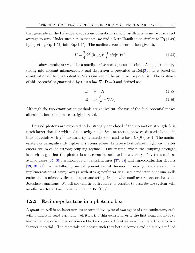
24 1. GENERAL INTRODUCTION TO QUANTUM FLUIDS OF LIGHT
inside the well: the bottom of the well’s conduction band is at a lower energy than in thesurrounding material and the bottom of its valence band at a higher energy (see Fig.(1.1)).The motion of carriers being confined in the plane of the well, a quantum well is essentiallya two-dimensional structure.
Figure 1.1: Energy of quantum states confined in a quantum well as a function of theposition along the growth direction Oz. V B is the valence band and CB the conductionband. Dashed lines represent energy levels. Eg denotes the energy gap and L the width ofthe well.
Due to Coulomb interaction, a hole of the valence band and an electron of the conductionband can form an hydrogen-like bound state called “exciton”. The creation of such (quasi)-bosonic excitation corresponds to the lowest energy optical transition of the quantum well.
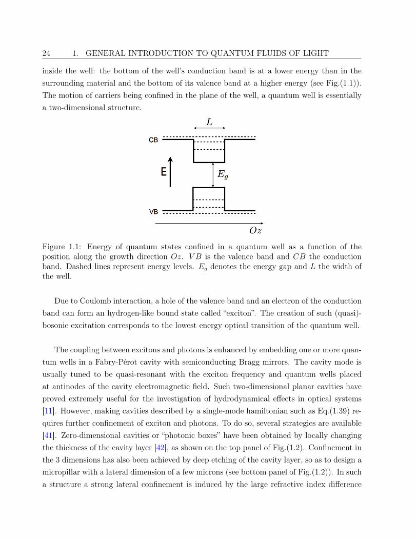
The coupling between excitons and photons is enhanced by embedding one or more quan-tum wells in a Fabry-Pérot cavity with semiconducting Bragg mirrors. The cavity mode isusually tuned to be quasi-resonant with the exciton frequency and quantum wells placedat antinodes of the cavity electromagnetic field. Such two-dimensional planar cavities haveproved extremely useful for the investigation of hydrodynamical effects in optical systems[11]. However, making cavities described by a single-mode hamiltonian such as Eq.(1.39) re-quires further confinement of exciton and photons. To do so, several strategies are available[41]. Zero-dimensional cavities or “photonic boxes” have been obtained by locally changingthe thickness of the cavity layer [42], as shown on the top panel of Fig.(1.2). Confinement inthe 3 dimensions has also been achieved by deep etching of the cavity layer, so as to design amicropillar with a lateral dimension of a few microns (see bottom panel of Fig.(1.2)). In sucha structure a strong lateral confinement is induced by the large refractive index difference
Strongly Correlated Photons in Arrays of Nonlinear Cavities 25
between air and semiconductors.
Figure 1.2: Top panels: photonic box from a microcavity with position-dependent thick-ness. (a) Scheme of a cavity with circular mesa etched on the spacer layer. (b) Schemeof the potential trap with two confined levels. (c) AFM image of a 9-µm-diameter circularmesa on the surface of the top mirror [42]. Bottom panel: coupled micropillars designed atLaboratoire de Photonique et Nanostructures in Marcoussis (France).
If the confinement is sufficiently strong, the energy spacing between confined modes ofthe field is much larger that the mode spectral width. It can also be much larger than thedetuning between the pump and the excitonic frequency. Under such circumstances, it is safeto consider only a single photonic mode and a single excitonic level [43]. The Hamiltonian(without external driving) then reads:
Hexc−ph = ~ωXd†d+ ~ωCa†a+ ~ΩR(d†a+ a†d) +~ωnl
2d†d†dd, (1.57)
where ~ωX is the exciton energy, ~ωC the photon energy, ~ΩR the coupling constant (Rabienergy) and ~ωnl the exciton-exciton interaction. The operator a† creates a photon in thecavity mode and d† an exciton.
26 1. GENERAL INTRODUCTION TO QUANTUM FLUIDS OF LIGHT
To begin with, let us first consider the quadratic part of the Hamiltonian: ~ωXd†d +
~ωCa†a+ ~ΩR(d†a+ a†d).It can be readily diagonalized by performing a unitary transformation on the operators a†
and d†. The new operators create and annihilate hybrid ligh-matter bosonic quasiparticlescalled exciton-polaritons. This polaritonic creation and destruction operators are given by:
(p†1
p†2
)=
(X C
−C X
)(d†
a†
). (1.58)
The coefficients X and C are respectively the polariton excitonic and photonic ampltudes.They obey a normalization condition: X2 + C2 = 1.
The polaritonic modes have frequencies
ω± =ωX + ωC
2±√
ΩR + (ωX − ωC
2)2. (1.59)
The lowest of these frequencies is denoted by ωLP and corresponds to the lower polaritonbranch. With these notations, excitonic and photonic amplitudes read:
C = − 1√1 + (ωLP−ωC
ΩR)2, X =
1√1 + ( ΩR
ωLP−ωC)2. (1.60)
Before rewriting the Hamiltonian of Eq.(1.57) as a function of polaritonic operators, auseful simplification may be introduced if the laser frequency is chosen to be quasi-resonantwith the lower polariton branch: one can neglect the effect of the upper branch and discardall terms containing p2 and p†2. The Hamiltonian then reads:
Hexc−ph = ~ωLPp†1p1 +
~ωnl2X4p†1p
†1p1p1. (1.61)
We see that this Hamiltonian is once again similar to Eq.(1.39). This is another example,treated at a more microscopic level, of effective interactions between dressed photons inducedby the coupling of light to a nonlinear medium.
1.2.3 Example of nonlinear resonators in circuit QED
Other very promising candidates for the experimental implementation of cavity arrays withlarge nonlinearities come from the relatively young, but prominent field of circuit quantumelectrodynamics (circuit QED). The nonlinear elements are this time superconducting cir-cuits with Josephson junctions and the role of the Fabry-Pérot cavity is played by microwave

Strongly Correlated Photons in Arrays of Nonlinear Cavities 27
transmission line resonators. Since one of the major focus of the field is quantum informationprocessing, the nonlinear elements considered in most of the literature are two-level systems(qubits). From a theoretical point of view, the interaction of such qubits with microwavephotons is well described by the Jaynes-Cummings model. This model does share some simi-larities with the Kerr Hamiltonian that will be discussed in the next subsection. For now, letus take a different route and focus on a circuit that is actually modeled by a Kerr nonlinearity.
The superconducting circuits used in circuit QED are macroscopic objects, with a sizeranging from a hundred of microns to a few millimeters, and that behave quantum mechan-ically. Macroscopic variables such as currents or voltages are still the relevant degrees offreedom, but they are described by noncommuting operators. The general procedure em-ployed to derive Hamitonians for these circuits follows the rules of canonical quantizationand is therefore not very different from the one outlined earlier in this chapter. In partic-ular the mains steps remain the same: first, one must write an appropriate Lagrangian forthe classical circuit, the corresponding classical Hamiltonian is then obtained by means of aLegendre transform. Finally, quantization is achieved by imposing canonical commutationrelations to conjugate dynamical variables. Following Girvin [44], we first illustrate theserules on the circuit with the simplest dynamics: the LC resonator.
Basics in circuit quantization: The LC resonator
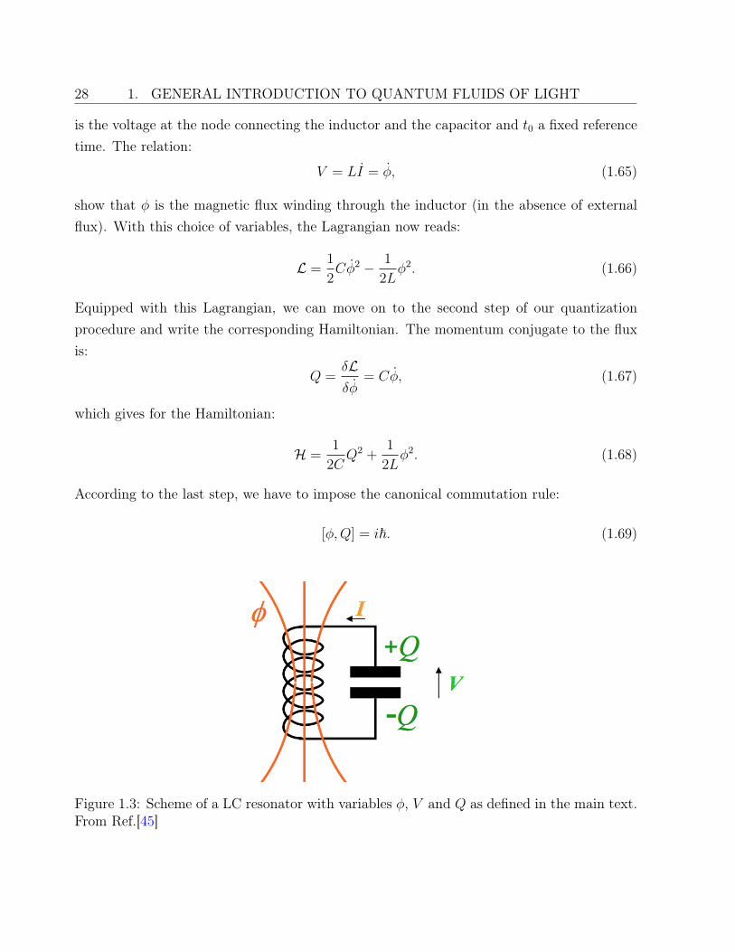
A natural choice of dynamical variables for a LC oscillator is the charge q accumulatedon the capacitor by the current I flowing through the circuit. The Lagrangian is then:
L =1
2Lq2 − 1
2Cq2. (1.62)
In this description the “kinetic part” is represented by the inductor while the “potentialenergy” is stored in the capacitor. For a reason that will become clear later when we includenonlinear elements in the circuit, it is more convenient to adopt an alternative point of viewand choose the node flux φ as a “position” variable. It is defined as follows:
φ(t) =
∫ t
t0
V (t′)dt′, (1.63)
where
V = − qC, (1.64)
28 1. GENERAL INTRODUCTION TO QUANTUM FLUIDS OF LIGHT
is the voltage at the node connecting the inductor and the capacitor and t0 a fixed referencetime. The relation:
V = LI = φ, (1.65)
show that φ is the magnetic flux winding through the inductor (in the absence of externalflux). With this choice of variables, the Lagrangian now reads:
L =1
2Cφ2 − 1
2Lφ2. (1.66)
Equipped with this Lagrangian, we can move on to the second step of our quantizationprocedure and write the corresponding Hamiltonian. The momentum conjugate to the fluxis:
Q =δLδφ
= Cφ, (1.67)
which gives for the Hamiltonian:
H =1
2CQ2 +
1
2Lφ2. (1.68)
According to the last step, we have to impose the canonical commutation rule:
[φ,Q] = i~. (1.69)
Figure 1.3: Scheme of a LC resonator with variables φ, V and Q as defined in the main text.From Ref.[45]
Strongly Correlated Photons in Arrays of Nonlinear Cavities 29
A nonlinear resonator
Capacitor and inductors are basic linear elements of a circuit. In particular, transmissionlines can be modeled by a chain of capacitors and inductors. As for nonlinear elements, theirbuilding block is the Josephson junction. Such a junction is formed by two superconductorsseparated by a thin layer of insulating material. It can be shown that under appropriateconditions, the Cooper pairs of the superconductors can tunnel through the insulating barrierwithout dissipation. Inserted in a circuit the Josephson junction acts as a nonlinear inductorgoverned by the two celebrated Josephson equations:
I = I0 sin δ, (1.70)dδ
dt=V
φ0
= V2e
~, (1.71)
with δ the difference between the phases of the two superconductors order parameter, V thevoltage applied to the junction and I0 a critical intensity depending on the superconductorenergy gap and on the resistance of the junction. We have also introduced the flux quantumφ0 = ~/2e.
Note that if we choose the set of variables defined in Eq.(1.62), where the “kinetic part”is represented by inductors and the “potential energy” by capacitors, the inclusion of aJosephson junction in the circuit would result in non-quadratic kinetic terms. Introducingthe flux variable as in Eq.(1.63) in order to avoid this complication, we find that the intensitycan be rewritten as:
I = I0 sin(φ
φ0
). (1.72)
The nonlinear inductance of the junction is characterized by
LJ =
(dI
dφ
)−1
=LJ0
cos( φφ0
), (1.73)
where LJ0 is the effective linear inductance of the junction, LJ0 = φ0/I0. Finally, in view ofwriting a Lagrangian for circuits containing Josephson junctions, we can compute the energystored in the junction, E(t) =
∫ t−∞ I(t′)V (t′)dt′, and find:
E(t) = −EJ cos(φ
φ0
), (1.74)
with EJ = I0φ0.
30 1. GENERAL INTRODUCTION TO QUANTUM FLUIDS OF LIGHT
The method of circuit quantization presented above can now be extended to more complexcircuits with n different nodes, with a Lagrangian L(φ1, φn, . . . , φ1, . . . , φn) depending on fluxvariables in the n nodes. The Lagrangian can be cast in the form L = T−V where T containsthe “kinetic energy” stemming from capacitors and V the “potential energy” that comes frominductors and Josephson junctions. The contribution of each type of element connecting thenodes n and n+ 1 has the form:
Tcapacitor =C
2(φn+1 − φn+1)2, (1.75)
Vinductor =1
2L(φn+1 − φn)2, (1.76)
VJJ = −EJ cos
((φn+1 − φn)
φ0
). (1.77)
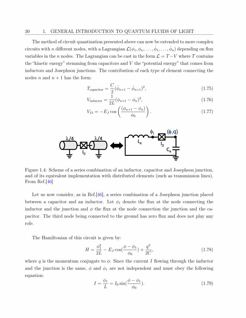
Figure 1.4: Scheme of a series combination of an inductor, capacitor and Josephson junction,and of its equivalent implementation with distributed elements (such as transmission lines).From Ref.[46]
Let us now consider, as in Ref.[46], a series combination of a Josephson junction placedbetween a capacitor and an inductor. Let φ1 denote the flux at the node connecting theinductor and the junction and φ the flux at the node connection the junction and the ca-pacitor. The third node being connected to the ground has zero flux and does not play anyrole.
The Hamiltonian of this circuit is given by:
H =φ2
1
2L− EJ cos(
φ− φ1
φ0
) +q2
2C, (1.78)
where q is the momentum conjugate to φ. Since the current I flowing through the inductorand the junction is the same, φ and φ1 are not independent and must obey the followingequation:
I =φ1
L= I0 sin(
φ− φ1
φ0
). (1.79)
Strongly Correlated Photons in Arrays of Nonlinear Cavities 31
This in turn defines a implicit relation between φ1 and φ, φ1 = g(φ). Injecting this lastexpression into the Hamiltonian and expanding it in powers of φ up to fourth order, we find:
H =φ2
2Lt+
q2
2Ce− 1
24
L3J0
L4tφ
20
φ4, (1.80)
with Lt the total inductance Lt = LJ0 + Le. Introducing now the creation and destructionoperators associated with φ and q:
φ = i
√~Ze
2(a− a†), (1.81)
q =
√~
2Ze(a+ a†), (1.82)
where the impedance Ze =√Lt/Ce, and keeping only the resonant terms, we get the Kerr
Hamiltonian:H = ~ω0a
†a+U
2a†a†aa, (1.83)
with
U = −e2ω0Ze
2
(LJ0
Lt
)3
, (1.84)
and ω0 = 1/√LtCe.
1.2.4 Kerr vs Jaynes-Cummings
As it was mentioned above, most of circuit-QED experiments focus on the interaction ofmicrowave photons with circuit elements forming a qubit, the latter being (up to a very goodapproximation) a two-level system. Under such circumstances, the most relevant effectivemodel to treat light-matter coupling is the Jaynes-Cummings model [47]. In the following,we briefly present its most important characteristics and compare it to the Kerr Hamiltonianof Eq.(1.39).
This model describes the interaction of a single mode of the electromagnetic field witha two level-system, which has a ground state |g〉 and an excited state |e〉. The Jaynes-Cummings Hamiltonian is the following:
HJC = ~ω0|e〉〈e|+ ~ωca†a+ i~Ω
2(a†|g〉〈e| − a|e〉〈g|), (1.85)
where a is, as usual the annihilation operator for photons, ωc the frequency of the corre-sponding mode, ~ω0 the energy of the state |e〉 and Ω the Rabi frequency of light-mattercoupling.
32 1. GENERAL INTRODUCTION TO QUANTUM FLUIDS OF LIGHT
If one tries to derive such a Hamiltonian from first principles, one will realize that allnonresonant terms were neglected. This rotating wave approximation is valid provided thatthe Rabi frequency Ω is much smaller than ω0 and ωc. In the so-called “ultrastrong couplingregime”, where Ω ∼ ω0, ωc, these nonresonant terms play a crucial role [48, 49, 50]. However,in the following, we will always consider the regime Ω ω0, ωc and we will thus neglecttheir effect. We mention this approximation primarily to emphasize one of its consequences,namely that the total number of excitations (photonic + matter-like) is conserved. In otherwords, the subspacesMn generated by two states of the form |n, g〉 and |n− 1, e〉 are closedunder the action of HJC.
As a result, the full energy spectrum of HJC is obtained by diagonalizing its restrictionto each of the Mn subspaces. The eigenstates of the resulting 2 × 2 Hamiltonians are thefollowing [51]:
|Ψ+,n〉 = cos θn|g, n〉+ i sin θn|e, n− 1〉, (1.86)
|Ψ−,n〉 = i sin θn|g, n〉+ cos θn|e, n− 1〉, (1.87)
with:tan 2θn =
−Ω√n
δ0 ≤ θn < π/2, (1.88)
andδ = ωc − ω0. (1.89)
The energy of these states is:
E±,n = n~ωc −δ
2± 1
2
√nΩ2 + δ2. (1.90)
As in Eq.(1.58), |Ψ±,n〉 are hybrid light-matter eigenstates and are also called dressed states.
If the Rabi frequency goes to zero while the detuning δ remains positive, then θn → 0
and we recover that within the subspaceMn, the ground state is
|Ψ−,n〉 = |e, n− 1〉, (1.91)
with the energy E−,n = n~ωc− δ. In the opposite case of negative detuning, we see from thecondition 0 < θ < π/2, that θ → π/2, and as expected the ground state is
|Ψ−,n〉 = |g, n〉, (1.92)
Strongly Correlated Photons in Arrays of Nonlinear Cavities 33
and the corresponding energy E−,n = n~ωc.The photonic and matter parts of the dressed states are equal (up to a phase) when the
cavity mode is at resonance with the e → g transition (δ = 0). In this case the energydifference, or vacuum Rabi splitting, between the two dressed levels is :
E+,n − E−,n =√nΩ. (1.93)
As it can be seen from Eq.(1.90), Kerr and Jaynes-Cummings spectra are, generallyspeaking, different [52]. The latter can nonetheless be mapped into the former, up to acertain value of n0, in the limit of large detuning n0Ω |δ|. For example, in the case of alarge negative detuning, the lowest energy states |Ψ−,n〉 are almost purely photonic and aTaylor expansion of their energy gives:
E−,n = n~ω′ +U ′
2n(n− 1), (1.94)
with an effective cavity frequency
~ω′ = ~ωc −Ω2
4|δ| , (1.95)
and a nonlinearity
U ′ =Ω4
8|δ|3 . (1.96)
To compare the two models outside of this mapping, it is convenient to define a effectivenonlinearity for the Jaynes-Cummings model as
Ueff = E−,2 − 2E−,1. (1.97)
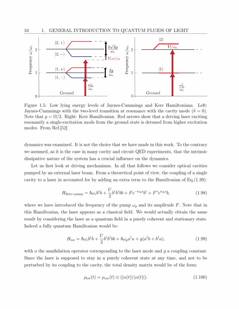
An example of energy levels of the two models illustrating this definition is shown onFig.(1.5). As we shall see when discussing the “photon blockade ”, this quantity is particularlyrelevant in the regime where only a few excited states are populated (e. g., n = 0, 1, 2).
1.2.5 Drive and dissipation
We have so far deliberately ignored the issue of driving and dissipation in our description ofa cavity. Of course, since the number of photons is not conserved, a pump-loss mechanismof some sort is always at play in optical systems. As we will see at the end of this chapter,the first theoretical investigations of cavity arrays neglected the effects of dissipation on thetime scale of simulations (and potential experiments). As a result, only quasi-equilibrium
34 1. GENERAL INTRODUCTION TO QUANTUM FLUIDS OF LIGHT
Figure 1.5: Low lying energy levels of Jaynes-Cummings and Kerr Hamiltonians. Left:Jaynes-Cummings with the two-level transition at resonance with the cavity mode (δ = 0).Note that g = Ω/2. Right: Kerr Hamiltonian. Red arrows show that a driving laser excitingresonantly a single-excitation mode from the ground state is detuned from higher excitationmodes. From Ref.[52]
dynamics was examined. It is not the choice that we have made in this work. To the contrarywe assumed, as it is the case in many cavity and circuit QED experiments, that the intrinsicdissipative nature of the system has a crucial influence on the dynamics.
Let us first look at driving mechanisms. In all that follows we consider optical cavitiespumped by an external laser beam. From a theoretical point of view, the coupling of a singlecavity to a laser in accounted for by adding an extra term to the Hamiltonian of Eq.(1.39):
HKerr+pump = ~ωcb†b+U
2b†b†bb+ Fe−iωptb† + F ∗eiωptb, (1.98)
where we have introduced the frequency of the pump ωp and its amplitude F . Note that inthis Hamiltonian, the laser appears as a classical field. We would actually obtain the sameresult by considering the laser as a quantum field in a purely coherent and stationary state.Indeed a fully quantum Hamiltonian would be:
Htot = ~ωcb†b+U
2b†b†bb+ ~ωpa†a+ g(a†b+ b†a), (1.99)
with a the annihilation operator corresponding to the laser mode and g a coupling constant.Since the laser is supposed to stay in a purely coherent state at any time, and not to beperturbed by its coupling to the cavity, the total density matrix would be of the form:
ρtot(t) = ρcav(t)⊗ (|α(t)〉〈α(t)|). (1.100)
Strongly Correlated Photons in Arrays of Nonlinear Cavities 35
Besides the evolution of α(t) must be governed by free field equations, which gives:
α(t) = 〈a(t)〉 = α0e−iωpt. (1.101)
Tracing over the laser mode in the Liouville-von Neumann equation [53]
i∂tρtot =1
~[Htot, ρtot], (1.102)
we recover the Hamiltonian of Eq.(1.98) with F = gα0 for the cavity.
The choice of a coherent pumping is not the only possible scenario. For example, a lotof works have been devoted to dissipative Bose-Einstein condensates of polaritons underincoherent pumping. As we will see shorty, one of the fundamental differences between thesetwo choices is that U(1) gauge invariance is preserved in the Hamiltonian under incoherentpumping while it is broken explicitly by a coherent pump.
Let us now turn to dissipation. Spontaneous emission processes originate from the cou-pling of the cavity mode to the external vacuum modes. This infinite collection of modesact as a Markovian bath of harmonic oscillators. Under appropriate approximation a masterequation for the cavity density matrix can be derived by starting from the Liouville-vonNeumann equation and tracing over the bath [27]. In contrast with the driving field, dissipa-tion will not be included in the Hamiltonian, since its most important effect is to break theunitarity of the system dynamics. As it is usually the case in quantum optics, the resultingmaster equation can be cast into a canonical Linblad form and expressed as:
i∂tρcav =1
~[HKerr+pump, ρcav] +
iγ
2[2bρcavb
† − b†bρcav − ρcavb†b], (1.103)
where γ is the cavity loss rate. The main goal of this thesis is to find the stationary solutionsof Eq.(1.103) extended to arrays of cavities.
1.2.6 Effective Hamiltonian for nonlinear cavity arrays
At this point we have at our disposal all the necessary ingredients for writing down aneffective Hamiltonian and a master equation for the full array of coupled cavities. Photonhopping is allowed by evanescent coupling of neighboring cavities due to their proximity. Itis included in the Hamiltonian in the from of:
Hhop = −J∑
〈i,j〉
b†ibj, (1.104)
36 1. GENERAL INTRODUCTION TO QUANTUM FLUIDS OF LIGHT
where 〈i, j〉 indicates that the sum runs over first neighbors only. Bringing Eq.(1.104) to-gether with single-cavity Kerr Hamiltonians, we obtain the driven-dissipative Bose-Hubbardmodel:
H = −Jz
∑
<i,j>
b†ibj +N∑
i=1
~ωcb†ibi +N∑
i=1
U
2b†ib†ibibi +
N∑
i=1
(Fe−iωptb†i + F ∗eiωptbi), (1.105)
where N is the number of cavities and z the lattice coordination number (number of nearestneighbors). The corresponding master equation is:
i∂tρ =1
~[H, ρ] +
iγ
2
N∑
i=1
(2biρb†i − b†ibiρ− ρb†ibi). (1.106)
The first thing to be noticed about Eq.(1.105) is that it is time-dependent. It is convenientto eliminate this time dependence by performing a unitary transformation on the densitymatrix:
ρ→ UρU †, (1.107)
where U = eiωpt∑i b†i bi . This amounts to writing the density matrix in a frame rotating at the
pump frequency ωp. In this rotating frame, the general Linblad form of the master equationremains the same but the Hamiltonian governing the dynamics is now time independent:
Hrf = −Jz
∑
<i,j>
b†ibj −N∑
i=1
~∆ωb†ibi +N∑
i=1
U
2b†ib†ibibi +
N∑
i=1
(Fb†i + F ∗bi). (1.108)
We have introduced the detuning between the pump the bare cavity frequency ∆ω = ωp−ωc.From now on, we will be exclusively studying this rotating frame Hamiltonian.
Note that the chemical potential µ, which is a key quantity for equilibrium quantumgases, is replaced in this non-equilibrium model by three other parameters, F , ∆ω and γ.This substantially enlarges the parameter space.
Before starting to investigate in details the model described by Eq.(1.108) and Eq.(1.106)(which will be the focus of the remaining chapters), we first discuss some of the most impor-tant results regarding nonlinear cavity arrays that have been obtained recently. We beginby presenting the phenomenon that has triggered a lot of these works: the photon blockade.
1.3 Photon blockade
A blockade effect analogous to the Coulomb blockade of electrons in mesoscopic quantumdots [54], occurs in a nonlinear optical cavity when the presence of a single photon is sufficient
Strongly Correlated Photons in Arrays of Nonlinear Cavities 37
to inhibit the absorption of a second one. This spectacular effect is therefore one of the mosteloquent example of strong quantum correlations in optical systems. In terms of photonemission, it means that in the ideal case, it is impossible for the cavity to emit two photons atthe same time. A perfect photon blockade thus yields perfect antibunching, i.e., g(2)(0) = 0.
1.3.1 Photon blockade in Kerr and Jaynes-Cummings
Hamiltonians
In an optical system described by the Kerr or Jaynes-Cummings Hamiltonian, the photonblockade originates from a very large photon-photon interaction. In both models, the nonlin-earity between the lowest-energy single-photon state and the lowest-energy two-photon stateis given by |E2−2E1|, where E1 and E2 are the energies of the single-photon and two-photonstates respectively. If this energy shift is much larger than the line width ~γ of the energylevels, an external laser field tuned at the single-photon frequency will not be able to injecta second photon inside the cavity. In the case of the Kerr Hamiltonian, the nonlinearitydefined above is given directly by the parameter U and the condition for photon blockadethen reads
U/(~γ) 1. (1.109)
In the Jaynes-Cummings model, this relation becomes Ω/(~γ) 1, since in this case thenonlinearity is given by Ω(1−
√2/2).
Although the principles underlying the photon blockade seem relatively simple, its exper-imental observation is a real challenge. Indeed, the strength of the effective photon-photoninteraction is always the most crucial parameter when discussing experiments on quantumfluids of light and reaching high enough nonlinearities is non trivial. In this context, thetheoretical proposal of Imamoglu et al. [55] was an important milestone. Using a morecomplex model than the ones outlined above they showed that the photon blockade regimecould be reached using a gas of 4-level atoms as a nonlinear medium. Before discussing inmore details the mechanism responsible of photon-photon interactions in this proposal, let usmention that, regarding the photon blockade with Jaynes-Cummings nonlinearities, spectac-ular results have been obtained more recently with superconducting circuits [56] and singleatoms in optical cavities [57]. Possible observation of photon blockade in semiconductormicrocavities was also proposed by Verger et al.[43].
38 1. GENERAL INTRODUCTION TO QUANTUM FLUIDS OF LIGHT
1.3.2 Giant Kerr effect with 4-level atoms
The medium considered by Imamoglu et al. [55] was an assembly of 4-level atoms embeddedin a optical cavity. A scheme of the atomic levels is presented in Fig.(1.6). They form aΛ shape with one extra level and the frequencies of the 3 → 4 and 1 → 3 transitions areassumed to be close to the cavity frequency. In addition, the 2→ 3 transition is driven by anonperturbative external laser field. In order to grasp the meaning of this choice let us firstgo back to the more general phenomenon of Kerr nonlinearities in a standard 3-level system.
Let the atoms under consideration have a ground state |a〉, an intermediate state |b〉 anda final state |c〉. In the most general case, the |a〉 → |b〉 transition is addressed by a pumplaser with a coupling Rabi frequency Ωp and the |b〉 → |c〉 transition by a signal field witha coupling frequency Ωs (see right panel of Fig.(1.6)) In the proposal of Ref.[55], signal andpump fields are in fact the same incident field. The nonlinear susceptibility χ(3) is deducedfrom the atomic polarization:
P (t) =〈er〉V
, (1.110)
which is in turn computed by solving the Bloch equations for the atoms perturbatively inthe fields. The real part of χ(3), which is responsible for photon-photon interactions, is givenby:
Re[χ(3)3−level] =
|dab|2|dbc|2ρ8~3ε0
1
∆ω2ab∆ωbc
, (1.111)
where ρ is the atomic density, dab and dbc the dipole matrix elements of the transitions and∆ωab and ∆ωbc the detuning of the lasers with respect to these transitions.
What we learn from Eq.(1.111) is that in order for the nonlinearity to be high, the de-tunings should be small. There is however an intrinsic limitation to ∆ωab and ∆ωbc: theymust be much larger than the transitions width in order to avoid absorption.
It is however possible to overcome this limitation by using the 4-level system presentedabove. Indeed, one of the effects of the laser coupling the levels 2 and 3 is a drastic reductionof absorption, known as electromagnetically induced transparency [36]. It is a consequenceof an interference effect involving the two states dressed by the external field (see Fig.(1.6),right panel). In this 4-level scheme, the real part of the nonlinear susceptibility is given by:
Re[χ(3)4−level] =
|d13|2|d24|2ρ2~3ε0
1
Ω2c∆ω42
. (1.112)
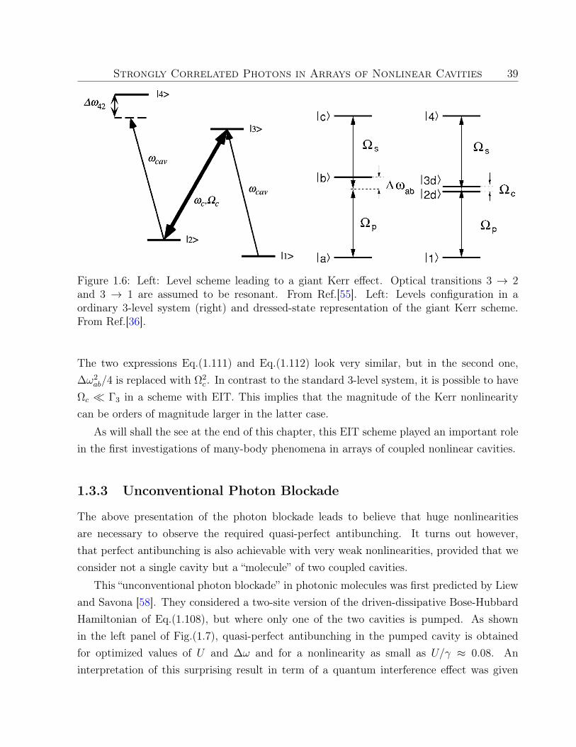
Strongly Correlated Photons in Arrays of Nonlinear Cavities 39
Figure 1.6: Left: Level scheme leading to a giant Kerr effect. Optical transitions 3 → 2and 3 → 1 are assumed to be resonant. From Ref.[55]. Left: Levels configuration in aordinary 3-level system (right) and dressed-state representation of the giant Kerr scheme.From Ref.[36].
The two expressions Eq.(1.111) and Eq.(1.112) look very similar, but in the second one,∆ω2
ab/4 is replaced with Ω2c . In contrast to the standard 3-level system, it is possible to have
Ωc Γ3 in a scheme with EIT. This implies that the magnitude of the Kerr nonlinearitycan be orders of magnitude larger in the latter case.
As will shall the see at the end of this chapter, this EIT scheme played an important rolein the first investigations of many-body phenomena in arrays of coupled nonlinear cavities.
1.3.3 Unconventional Photon Blockade
The above presentation of the photon blockade leads to believe that huge nonlinearitiesare necessary to observe the required quasi-perfect antibunching. It turns out however,that perfect antibunching is also achievable with very weak nonlinearities, provided that weconsider not a single cavity but a “molecule” of two coupled cavities.
This “unconventional photon blockade” in photonic molecules was first predicted by Liewand Savona [58]. They considered a two-site version of the driven-dissipative Bose-HubbardHamiltonian of Eq.(1.108), but where only one of the two cavities is pumped. As shownin the left panel of Fig.(1.7), quasi-perfect antibunching in the pumped cavity is obtainedfor optimized values of U and ∆ω and for a nonlinearity as small as U/γ ≈ 0.08. Aninterpretation of this surprising result in term of a quantum interference effect was given
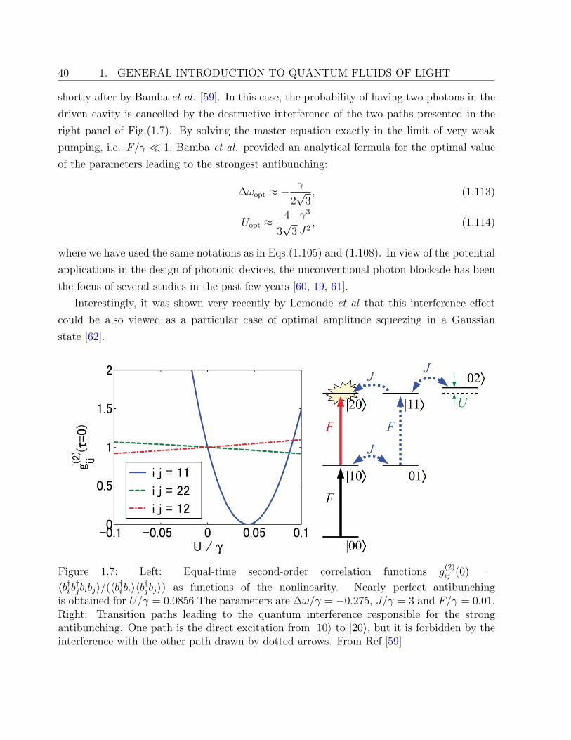
40 1. GENERAL INTRODUCTION TO QUANTUM FLUIDS OF LIGHT
shortly after by Bamba et al. [59]. In this case, the probability of having two photons in thedriven cavity is cancelled by the destructive interference of the two paths presented in theright panel of Fig.(1.7). By solving the master equation exactly in the limit of very weakpumping, i.e. F/γ 1, Bamba et al. provided an analytical formula for the optimal valueof the parameters leading to the strongest antibunching:
∆ωopt ≈ −γ
2√
3, (1.113)
Uopt ≈4
3√
3
γ3
J2, (1.114)
where we have used the same notations as in Eqs.(1.105) and (1.108). In view of the potentialapplications in the design of photonic devices, the unconventional photon blockade has beenthe focus of several studies in the past few years [60, 19, 61].
Interestingly, it was shown very recently by Lemonde et al that this interference effectcould be also viewed as a particular case of optimal amplitude squeezing in a Gaussianstate [62].
Figure 1.7: Left: Equal-time second-order correlation functions g(2)ij (0) =
〈b†ib†jbibj〉/(〈b†ibi〉〈b†jbj〉) as functions of the nonlinearity. Nearly perfect antibunchingis obtained for U/γ = 0.0856 The parameters are ∆ω/γ = −0.275, J/γ = 3 and F/γ = 0.01.Right: Transition paths leading to the quantum interference responsible for the strongantibunching. One path is the direct excitation from |10〉 to |20〉, but it is forbidden by theinterference with the other path drawn by dotted arrows. From Ref.[59]
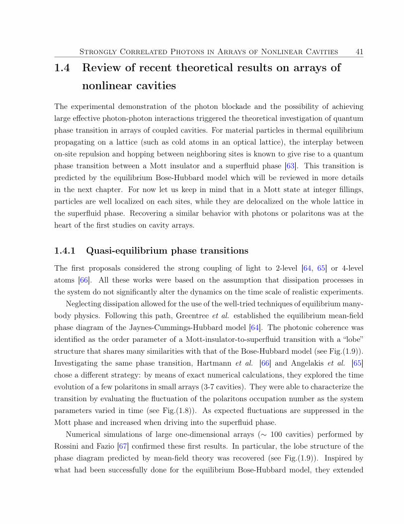
Strongly Correlated Photons in Arrays of Nonlinear Cavities 41
1.4 Review of recent theoretical results on arrays of
nonlinear cavities
The experimental demonstration of the photon blockade and the possibility of achievinglarge effective photon-photon interactions triggered the theoretical investigation of quantumphase transition in arrays of coupled cavities. For material particles in thermal equilibriumpropagating on a lattice (such as cold atoms in an optical lattice), the interplay betweenon-site repulsion and hopping between neighboring sites is known to give rise to a quantumphase transition between a Mott insulator and a superfluid phase [63]. This transition ispredicted by the equilibrium Bose-Hubbard model which will be reviewed in more detailsin the next chapter. For now let us keep in mind that in a Mott state at integer fillings,particles are well localized on each sites, while they are delocalized on the whole lattice inthe superfluid phase. Recovering a similar behavior with photons or polaritons was at theheart of the first studies on cavity arrays.
1.4.1 Quasi-equilibrium phase transitions
The first proposals considered the strong coupling of light to 2-level [64, 65] or 4-levelatoms [66]. All these works were based on the assumption that dissipation processes inthe system do not significantly alter the dynamics on the time scale of realistic experiments.
Neglecting dissipation allowed for the use of the well-tried techniques of equilibrium many-body physics. Following this path, Greentree et al. established the equilibrium mean-fieldphase diagram of the Jaynes-Cummings-Hubbard model [64]. The photonic coherence wasidentified as the order parameter of a Mott-insulator-to-superfluid transition with a “lobe”structure that shares many similarities with that of the Bose-Hubbard model (see Fig.(1.9)).Investigating the same phase transition, Hartmann et al. [66] and Angelakis et al. [65]chose a different strategy: by means of exact numerical calculations, they explored the timeevolution of a few polaritons in small arrays (3-7 cavities). They were able to characterize thetransition by evaluating the fluctuation of the polaritons occupation number as the systemparameters varied in time (see Fig.(1.8)). As expected fluctuations are suppressed in theMott phase and increased when driving into the superfluid phase.
Numerical simulations of large one-dimensional arrays (∼ 100 cavities) performed byRossini and Fazio [67] confirmed these first results. In particular, the lobe structure of thephase diagram predicted by mean-field theory was recovered (see Fig.(1.9)). Inspired bywhat had been successfully done for the equilibrium Bose-Hubbard model, they extended
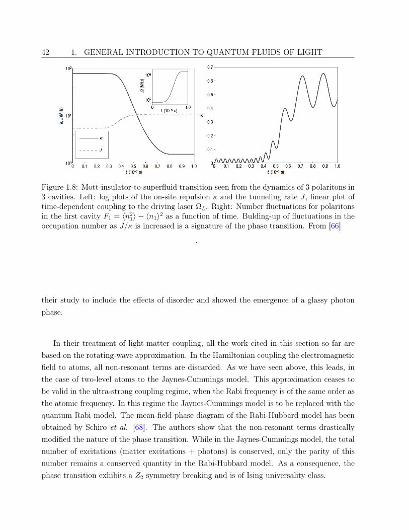
42 1. GENERAL INTRODUCTION TO QUANTUM FLUIDS OF LIGHT
Figure 1.8: Mott-insulator-to-superfluid transition seen from the dynamics of 3 polaritons in3 cavities. Left: log plots of the on-site repulsion κ and the tunneling rate J , linear plot oftime-dependent coupling to the driving laser ΩL. Right: Number fluctuations for polaritonsin the first cavity F1 = 〈n2
1〉 − 〈n1〉2 as a function of time. Bulding-up of fluctuations in theoccupation number as J/κ is increased is a signature of the phase transition. From [66]
.
their study to include the effects of disorder and showed the emergence of a glassy photonphase.
In their treatment of light-matter coupling, all the work cited in this section so far arebased on the rotating-wave approximation. In the Hamiltonian coupling the electromagneticfield to atoms, all non-resonant terms are discarded. As we have seen above, this leads, inthe case of two-level atoms to the Jaynes-Cummings model. This approximation ceases tobe valid in the ultra-strong coupling regime, when the Rabi frequency is of the same order asthe atomic frequency. In this regime the Jaynes-Cummings model is to be replaced with thequantum Rabi model. The mean-field phase diagram of the Rabi-Hubbard model has beenobtained by Schiro et al. [68]. The authors show that the non-resonant terms drasticallymodified the nature of the phase transition. While in the Jaynes-Cummings model, the totalnumber of excitations (matter excitations + photons) is conserved, only the parity of thisnumber remains a conserved quantity in the Rabi-Hubbard model. As a consequence, thephase transition exhibits a Z2 symmetry breaking and is of Ising universality class.
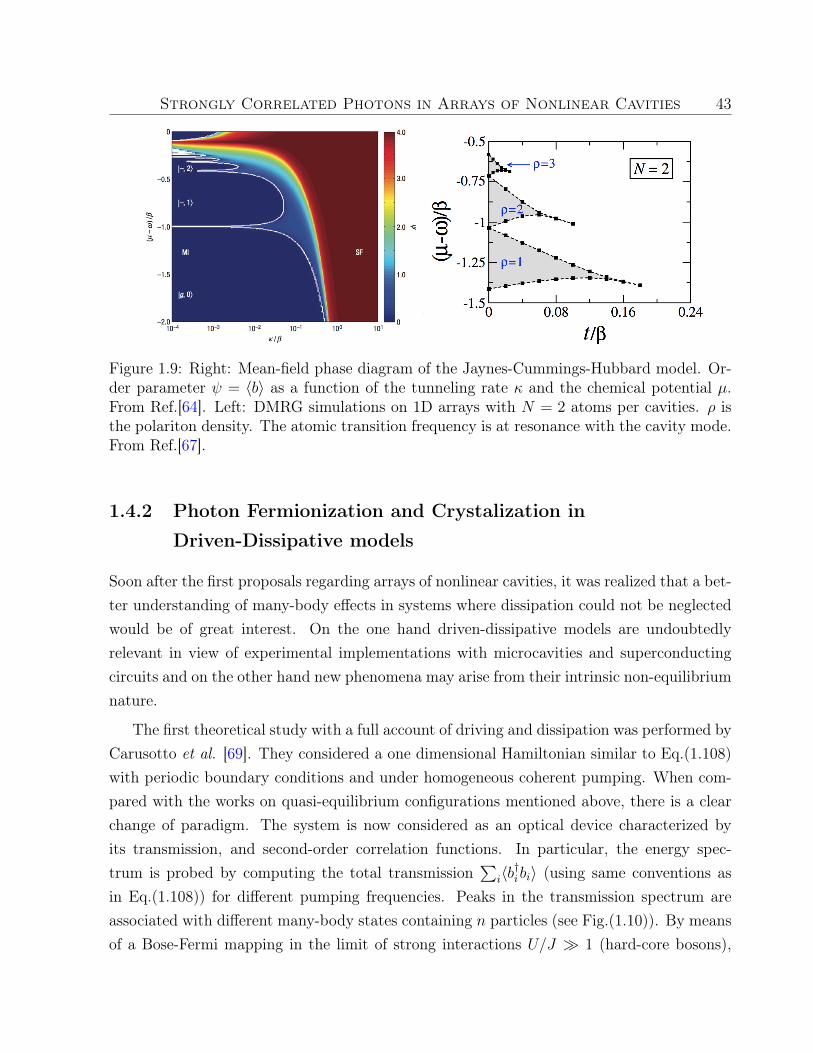
Strongly Correlated Photons in Arrays of Nonlinear Cavities 43
Figure 1.9: Right: Mean-field phase diagram of the Jaynes-Cummings-Hubbard model. Or-der parameter ψ = 〈b〉 as a function of the tunneling rate κ and the chemical potential µ.From Ref.[64]. Left: DMRG simulations on 1D arrays with N = 2 atoms per cavities. ρ isthe polariton density. The atomic transition frequency is at resonance with the cavity mode.From Ref.[67].
1.4.2 Photon Fermionization and Crystalization in
Driven-Dissipative models
Soon after the first proposals regarding arrays of nonlinear cavities, it was realized that a bet-ter understanding of many-body effects in systems where dissipation could not be neglectedwould be of great interest. On the one hand driven-dissipative models are undoubtedlyrelevant in view of experimental implementations with microcavities and superconductingcircuits and on the other hand new phenomena may arise from their intrinsic non-equilibriumnature.
The first theoretical study with a full account of driving and dissipation was performed byCarusotto et al. [69]. They considered a one dimensional Hamiltonian similar to Eq.(1.108)with periodic boundary conditions and under homogeneous coherent pumping. When com-pared with the works on quasi-equilibrium configurations mentioned above, there is a clearchange of paradigm. The system is now considered as an optical device characterized byits transmission, and second-order correlation functions. In particular, the energy spec-trum is probed by computing the total transmission
∑i〈b†ibi〉 (using same conventions as
in Eq.(1.108)) for different pumping frequencies. Peaks in the transmission spectrum areassociated with different many-body states containing n particles (see Fig.(1.10)). By meansof a Bose-Fermi mapping in the limit of strong interactions U/J 1 (hard-core bosons),
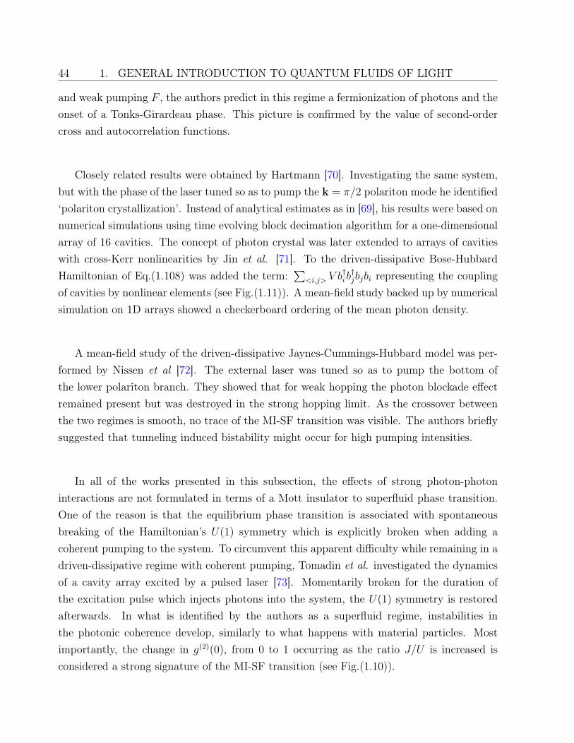
44 1. GENERAL INTRODUCTION TO QUANTUM FLUIDS OF LIGHT
and weak pumping F , the authors predict in this regime a fermionization of photons and theonset of a Tonks-Girardeau phase. This picture is confirmed by the value of second-ordercross and autocorrelation functions.
Closely related results were obtained by Hartmann [70]. Investigating the same system,but with the phase of the laser tuned so as to pump the k = π/2 polariton mode he identified‘polariton crystallization’. Instead of analytical estimates as in [69], his results were based onnumerical simulations using time evolving block decimation algorithm for a one-dimensionalarray of 16 cavities. The concept of photon crystal was later extended to arrays of cavitieswith cross-Kerr nonlinearities by Jin et al. [71]. To the driven-dissipative Bose-HubbardHamiltonian of Eq.(1.108) was added the term:
∑<i,j> V b
†ib†jbjbi representing the coupling
of cavities by nonlinear elements (see Fig.(1.11)). A mean-field study backed up by numericalsimulation on 1D arrays showed a checkerboard ordering of the mean photon density.
A mean-field study of the driven-dissipative Jaynes-Cummings-Hubbard model was per-formed by Nissen et al [72]. The external laser was tuned so as to pump the bottom ofthe lower polariton branch. They showed that for weak hopping the photon blockade effectremained present but was destroyed in the strong hopping limit. As the crossover betweenthe two regimes is smooth, no trace of the MI-SF transition was visible. The authors brieflysuggested that tunneling induced bistability might occur for high pumping intensities.
In all of the works presented in this subsection, the effects of strong photon-photoninteractions are not formulated in terms of a Mott insulator to superfluid phase transition.One of the reason is that the equilibrium phase transition is associated with spontaneousbreaking of the Hamiltonian’s U(1) symmetry which is explicitly broken when adding acoherent pumping to the system. To circumvent this apparent difficulty while remaining in adriven-dissipative regime with coherent pumping, Tomadin et al. investigated the dynamicsof a cavity array excited by a pulsed laser [73]. Momentarily broken for the duration ofthe excitation pulse which injects photons into the system, the U(1) symmetry is restoredafterwards. In what is identified by the authors as a superfluid regime, instabilities inthe photonic coherence develop, similarly to what happens with material particles. Mostimportantly, the change in g(2)(0), from 0 to 1 occurring as the ratio J/U is increased isconsidered a strong signature of the MI-SF transition (see Fig.(1.10)).
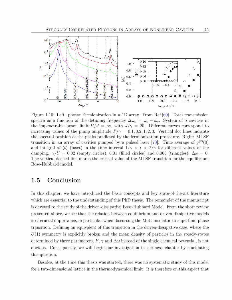
Strongly Correlated Photons in Arrays of Nonlinear Cavities 45
Figure 1.10: Left: photon fermionization in a 1D array. From Ref.[69]. Total transmissionspectra as a function of the detuning frequency ∆ωp = ωp − ωc. System of 5 cavities inthe impenetrable boson limit U/J = ∞, with J/γ = 20. Different curves correspond toincreasing values of the pump amplitude F/γ = 0.1, 0.2, 1, 2, 3. Vertical dot lines indicatethe spectral position of the peaks predicted by the fermionization procedure. Right: MI-SFtransition in an array of cavities pumped by a pulsed laser [73]. Time average of g(2)(0)and integral of 〈b〉 (inset) in the time interval 1/γ < t < 2/γ for different values of thedamping: γ/U = 0.02 (empty circles), 0.01 (filled circles) and 0.005 (triangles), ∆ω = 0.The vertical dashed line marks the critical value of the MI-SF transition for the equilibriumBose-Hubbard model.
1.5 Conclusion
In this chapter, we have introduced the basic concepts and key state-of-the-art literaturewhich are essential to the understanding of this PhD thesis. The remainder of the manuscriptis devoted to the study of the driven-dissipative Bose-Hubbard Model. From the short reviewpresented above, we see that the relation between equilibrium and driven-dissipative modelsis of crucial importance, in particular when discussing the Mott-insulator-to-superfluid phasetransition. Defining an equivalent of this transition in the driven-dissipative case, where theU(1) symmetry is explicitly broken and the mean density of particles in the steady-statesdetermined by three parameters, F , γ and ∆ω instead of the single chemical potential, is notobvious. Consequently, we will begin our investigation in the next chapter by elucidatingthis question.
Besides, at the time this thesis was started, there was no systematic study of this modelfor a two-dimensional lattice in the thermodynamical limit. It is therefore on this aspect that
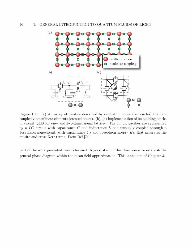
46 1. GENERAL INTRODUCTION TO QUANTUM FLUIDS OF LIGHT
Figure 1.11: (a) An array of cavities described by oscillator modes (red circles) that arecoupled via nonlinear elements (crossed boxes). (b), (c) Implementation of its building blocksin circuit QED for one- and two-dimensional lattices. The circuit cavities are representedby a LC circuit with capacitance C and inductance L and mutually coupled through aJosephson nanocircuit, with capacitance CJ and Josephson energy EJ , that generates theon-site and cross-Kerr terms. From Ref.[71].
part of the work presented here is focused. A good start in this direction is to establish thegeneral phase-diagram within the mean-field approximation. This is the aim of Chapter 3.
Chapter 2
Equilibrium vs driven-dissipativeBose-Hubbard model
When discussing results on the driven-dissipative Bose-Hubbard model with people fromthe cold-atom community, a question inevitably arises: “What happens in your model whenF and γ go both to zero?”. In this limit, it should indeed resemble more and more toits better-known equilibrium counterpart. Exploring the regime of weak pumping and weakdissipation seems therefore a good way to clarify the relation between the two models. Beforeembarking on this investigation, we will review some important results on the equilibriumBose-Hubbard model.
Originally introduced by Hubbard for the understanding of electron transport in met-als [74], its study for bosonic particles was first carried out in 1989 in a seminal paper byFisher et al. [63]. Using mean-field theory, they predicted the celebrated Mott-insulator-to-superfluid transition that we have already encountered in the preceding chapter. Theunderstanding of this phase transition was subsequently deepened by numerous theoreticalstudies using various methods, such as the random phase approximation [75], strong-couplingexpansions [76, 77, 78] or dynamical mean-field theory [79]. This model gained a renewed in-terest with the experimental observation of the transition with cold atoms in optical lattices[20]. In particular, the advent of efficient quantum Monte-Carlo algorithms for equilibriumbosonic systems allowed for very accurate numerical simulations [80, 81]. All these worksconfirmed that the results of mean-field theory were qualitatively correct.
After reviewing the mean-field phase diagram of the equilibrium Bose-Hubbard model, wewill extend this approach to the driven-dissipative model and present our results concerningthe regime of weak pumping and weak dissipation. Instead of pure Mott insulator states, wefind statistical mixtures with the same second-order coherence g(2)(0) as a Fock state with n
47
48 2. EQUILIBRIUM VS DRIVEN-DISSIPATIVE BOSE-HUBBARD MODEL
photons, but a mean photon number of n/2. These mixed states occur when n pump photonshave the same energy as n interacting photons inside the nonlinear cavity and survive upto a critical tunneling coupling strength, above which a crossover to classical coherent statetakes place. The original results presented in this chapter are published in [22].
Strongly Correlated Photons in Arrays of Nonlinear Cavities 49
2.1 Bose-Hubbard model at equilibrium
In this first section we derive the mean-field phase diagram of the equilibrium Bose-Hubbardmodel. This will give us the opportunity to go over the main features of the Mott-insulator-to-superfluid phase transition and to introduce important methods that will be extended todriven-dissipative systems.
For material particles in thermal equilibrium, the grand-canonical Bose-Hubbard Hamil-tonian is the following (~ = 1):
Heq = −Jz
∑
<i,j>
b†ibj +N∑
i=1
U
2b†ib†ibibi −
N∑
i=1
µb†ibi. (2.1)
We recognize the parameters J and U introduced previously. As for µ, it denotes thechemical potential. In this thesis, we will only consider the repulsive model, with U > 0.The physical meaning of U in this context appears more clearly when the repulsion term iswritten as a function of the number operator ni: 1
2b†ib†ibibi = 1
2ni(ni − 1). The right-hand
side of this last equation gives the number of pairs of particles at site i. The parameter U isthus the energy cost of on-site pair formation.
2.1.1 Two simple limits: J = 0 and U = 0
As all the interesting physics in this model stems from the competition between the kineticpart of the Hamiltonian governed by J and the on-site repulsion characterized by U , it isinstructive to look at the two limiting cases J = 0 and U = 0.
Isolated “Hubbard atoms”
For J = 0, all the sites are decoupled and may be seen as individual “Hubbard atoms”.The Hamiltonian reads:
∑
i
U
2ni(ni − 1)−
∑
i
µni. (2.2)
It is diagonal in real space. At zero temperature, the ground state is therefore a tensorproduct of the form:
|ψ〉MI =⊗
i
|n〉i, (2.3)
50 2. EQUILIBRIUM VS DRIVEN-DISSIPATIVE BOSE-HUBBARD MODEL
where n is the number of particles per site, whose value is fixed by the chemical potentialµ. The energy of each Hubbard atom is:
E(0)n = −µn+
1
2n(n− 1)U. (2.4)
Thus the ground state in the atomic limit is a so called Mott insulator, with the particlesperfectly localized on each site and without any fluctuations in the occupation number.It is useful to compute the energy required, in such a state, for a particle to move from onesite to the next:
∆E = E(n+ 1) + E(n− 1)− 2E(n)
=U
2(n(n+ 1) + (n− 1)(n− 2)− 2n(n− 1)) (2.5)
= U. (2.6)
This confirms the physical interpretation of U given above.
Freely propagating particles
In the opposite case where U = 0 the Hamiltonian becomes:
− J
z
∑
<i,j>
b†ibj −N∑
i=1
µni. (2.7)
It is not diagonal in real space anymore, but it is in reciprocal space. The ground stateis then a state with all the particles condensed in the one-particle zero-momentum state|k = 0〉. In real space, the state of the system reads:
|ψ〉SF =1√N !
(1√M
N∑
i=1
b†i
)N
|0〉, (2.8)
where N is the total number of particles and M the number of lattice sites. It is clearfrom the expression for |ψ〉SF that in this state, contrary to the preceding case, particlesare delocalized on the entire lattice and that on a given lattice site, the number of particlesfluctuates.
It is interesting to notice that in the thermodynamical limit N → ∞, the state |ψ〉SFcan be approximately written as a tensor product of coherent states on each site [82]:
|ψ〉SF ≈⊗
i
|α〉i, (2.9)
Strongly Correlated Photons in Arrays of Nonlinear Cavities 51
the parameter α being the same on each site, and such that |α|2 is equal to the mean particledensity.
2.1.2 Mean-field phase diagram
Equations (2.3) and (2.9) indicate that in both limits J = 0 and U = 0, the ground state isfactorized, that is, a tensor product of single-site states. This encourages to try a variationalapproach to the general problem [83]. Let us assume that the total ground state takes theform of a Gutzwiller ansatz:
|ψ〉GS =N⊗
i=1
|φ〉. (2.10)
The problem is then reduced to finding the state |φ〉 that minimizes the energy. The virtueof this approximation is that it reduces the original many-body problem to a single-siteproblem. The effective Hamiltonian Hmf for |φ〉 is derived by injecting Eq.(2.10) into thegeneral Schrödinger equation and projecting it on a single site. This procedure is actuallyequivalent to a decoupling of the sites directly inside the total Hamiltonian Heq. Indeed, theapproximation:
b†ibj ≈ 〈b†i〉bj + 〈bj〉b†i − 〈b†i〉〈bj〉, (2.11)
which is typical of mean-field theories, yields the same effective single-site Hamiltonian,namely:
Hmf = −µb†b+U
2b†b†bb− J〈b〉∗b− J〈b〉b†. (2.12)
From here, the idea is to start from the ground state at J = 0 and to treat the source termdue to the hopping appearing in Eq.(2.12) as a perturbation.
Let n be an integer such that µ/U ∈ [n − 1, n]. As seen in the previous subsection, theground state is |n〉, with the corresponding energy E(0)
n . Since our primary goal is to writea self-consistent equation for 〈b〉, we need to determine the perturbed eigenstates |φn〉 andcompute 〈φn|b|φn〉. Operators b and b† only couple |n〉 to |n − 1〉 and |n + 1〉 respectively.At first order, the expansion of |φn〉 in the unperturbed Fock basis is therefore:
|φn〉 = cn−1|n− 1〉+ cn|n〉+ cn+1|n+ 1〉, (2.13)
and the expression for 〈b〉 is:
〈φn|b|φn〉 =√ncnc
∗n−1 +
√n+ 1cn+1c
∗n. (2.14)
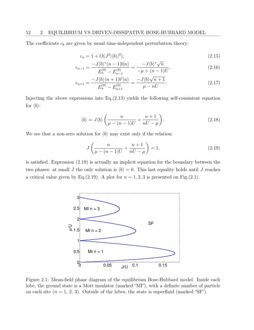
52 2. EQUILIBRIUM VS DRIVEN-DISSIPATIVE BOSE-HUBBARD MODEL
The coefficients ck are given by usual time-independent perturbation theory:
cn = 1 +O(J2|〈b〉|2), (2.15)
cn−1 =−J〈b〉∗〈n− 1|b|n〉
E(0)n − E(0)
n−1
=−J〈b〉∗√n−µ+ (n− 1)U
, (2.16)
cn+1 =−J〈b〉〈n+ 1|b†|n〉E
(0)n − E(0)
n+1
=−J〈b〉
√n+ 1
µ− nU . (2.17)
Injecting the above expressions into Eq.(2.13) yields the following self-consistent equationfor 〈b〉:
〈b〉 = J〈b〉(
n
µ− (n− 1)U+
n+ 1
nU − µ
). (2.18)
We see that a non-zero solution for 〈b〉 may exist only if the relation:
J
(n
µ− (n− 1)U+
n+ 1
nU − µ
)= 1, (2.19)
is satisfied. Expression (2.19) is actually an implicit equation for the boundary between thetwo phases: at small J the only solution is 〈b〉 = 0. This last equality holds until J reachesa critical value given by Eq.(2.19). A plot for n = 1, 2, 3 is presented on Fig.(2.1).
0 0.05 0.1 0.150
0.5
1
1.5
2
2.5
3
J/U
µ/U
SF
MI n = 3
MI n = 2
MI n = 1
Figure 2.1: Mean-field phase diagram of the equilibrium Bose-Hubbard model. Inside eachlobe, the ground state is a Mott insulator (marked “MI”), with a definite number of particleon each site (n = 1, 2, 3). Outside of the lobes, the state is superfluid (marked “SF”).
Strongly Correlated Photons in Arrays of Nonlinear Cavities 53
It is convenient to study the phase diagram in the (µ/U, J/U)-plane and write J = J/U
; µ = µ/U . Equation (2.19) expressed in terms of these normalized variables can be writtenas:
J =(µ− n+ 1)(n− µ)
µ+ 1. (2.20)
The maximal value of J on the boundary is given by the condition dJdµ
= 0. This yields:
µm =√n(n+ 1)− 1, (2.21)
Jm =1
(√n+√n+ 1)2
. (2.22)
Note that µm < n−1/2, which reflects the fact that the lobes are not symmetric with respectto µ = n− 1/2. Besides, Eq.(2.22) indicates that the size of the lobe shrinks as n increases.
2.2 Driven-dissipative model under weak pumping and
weak dissipation
While keeping in mind the results at equilibrium, we now turn to the driven-dissipative case.We recall that the Hamiltonian under consideration (in the rotating frame) is the following:
Hrf = −Jz
∑
<i,j>
b†ibj −N∑
i=1
~∆ωb†ibi +N∑
i=1
U
2b†ib†ibibi +
N∑
i=1
(Fb†i + F ∗bi), (2.23)
and that the dynamics is given by the master equation (1.106), characterized by a dissipationrate γ. In addition, we assume that F and γ are both very small when compared with thedetuning ∆ω. Without any loss of generality, we will also assume that F is real. The wayto proceed in order to find the steady-states will be the same as in the previous section: weconsider first the case of an isolated cavity with J = 0 and then treat the coupling betweensites within the mean-field approximation.
2.2.1 Single cavity: Analytical solution
At equilibrium, we have seen that the ground state of an isolated site is a pure Fock state |n〉,with n fixed by the value of the chemical potential. If we are to find some sort of equivalentin the driven-dissipative case, we must look for steady-states with a mean photon density〈b†b〉 ≥ 1. Since photon always have to be injected inside the cavity, and since in the presentcase the coupling to the external field is assumed to be very weak, the only way to have〈b†b〉 ≥ 1 is to be at resonance with multiphotonic absorption processes.
54 2. EQUILIBRIUM VS DRIVEN-DISSIPATIVE BOSE-HUBBARD MODEL
Multiphotonic resonances
Absorption of photons is resonantly enhanced when n incident laser photons have thesame energy as n photons inside the cavity. In the case of the Kerr Hamiltonian consideredso far, it means: nωp = nωc+Un(n−1)/2. Expressed in terms of the pump-cavity detuning,this relation reads:
U
∆ω=
2
n− 1. (2.24)
This energy matching condition can be satisfied for n > 1 only if ∆ω > 0. If the pump isresonant with the bare cavity frequency, i.e ∆ω = 0, only single photons can be absorbedresonantly. There is no relation between U and ∆ω in this case and the density matrix isfound by expanding the master equation in powers of F/U and γ/U . In the following, we willfocus on the more interesting case of multiphotonic resonances (n > 1) and assume ∆ω > 0.
For simplicity, let us first look at the two-photon resonance (U = 2∆ω). It appears thatin the rotating frame, the vacuum |0〉 has the same energy as the two photon-state |2〉 inthe absence of driving. This degeneracy is lifted by the coupling to the external field whoseeffect on the dynamics can be understood qualitatively in the following way. Suppose thatat time t = 0 the intra-cavity field is in the vacuum state |0〉. Since the vacuum is no longeran eigenstate of the rotating-frame Hamiltonian, but a linear combination of eigenstates
1√2(|0〉 + |2〉) and 1√
2(|0〉 − |2〉), the cavity field will start to oscillate between |0〉 and |2〉.
These Rabi oscillations will take place until the occurrence of a quantum jump, due to cavitylosses. After the emission of a first photon out of the cavity, the field is projected into thestate |1〉 and it is only after the emission of a second photon that it returns to vacuum.In that sense, the two-photon absorption process results, as expected, in the emission of aphoton “pair” out of the cavity. Since the single-photon state has a decay rate γ, the timebetween emission of photons from the same pair will be of the order of 1/γ.
If the frequency splitting between the two quasi-degenerate eigenstates is much smallerthan the dissipation rate, i.e. F 2/∆ω γ, the field will not have time to oscillate and willstay mostly in the vacuum state. In this low density regime, the average time required to ab-sorb a photon pair is much larger that the single-photon decay time 1/γ. Therefore, photonswill appear strongly bunched when compared with coherent light of the same intensity.
The time between successive pairs decreases with decreasing dissipation and photonbunching eventually disappears for F 2/∆ω γ. We will see quantitatively in the fol-lowing that the emitted light is even antibunched in this limit. Similar photon correlations
Strongly Correlated Photons in Arrays of Nonlinear Cavities 55
have also been predicted for the two-photon resonance of the Jaynes-Cummings model [84].
More quantitative results can be obtained by solving the master equation explicitly. Tofully grasp the effect of the resonance, we will assume that F/∆ω γ/∆ω. We will workis the basis formed by the eigenstates of the total Hamiltonian (up to the lowest order inF/∆ω), given by:
|a〉 =1√2
(|0〉+ |2〉), (2.25)
|b〉 =1√2
(|0〉 − |2〉), (2.26)
|c〉 = |1〉.
Since the driving term only couples Fock states |m〉 to |m ± 1〉, the coupling of |0〉 and |2〉is of order 2. The energies given by second-order perturbation theory are:
Ea 'F 2
∆ω(1 +
√2), (2.27)
Eb 'F 2
∆ω(1−
√2), (2.28)
Ec ' −∆ω. (2.29)
As expected, the energy splitting between states |a〉 and |b〉 is proportional to (F/∆ω)2. Inthe “dressed-state” basis, the dissipative term of the master equation couples populationsand coherences of the density matrix. However, in the lowest order in F/∆ω and γ/∆ω, thecoefficients ρac and ρbc vanish. The master equation in this basis reads:
∂tρaa = γ[1
2ρcc − ρaa +
1
2(ρab + ρba)], (2.30)
∂tρbb = γ[1
2ρcc − ρbb +
1
2(ρab + ρba)], (2.31)
∂tρab = ∆ω[(−i2√
2F 2
∆ω2− γ
∆ω)ρab +
γ
2∆ω], (2.32)
∂tρcc = γ[ρaa + ρbb − ρcc − (ρab + ρba)]. (2.33)
The stationary value for ρab is then:
ρab =1
2
1
1 + i2√
2F 2
γ∆ω
, (2.34)
giving:
ρab + ρba =1
1 + 8F 4
γ2∆ω2
= ξ. (2.35)
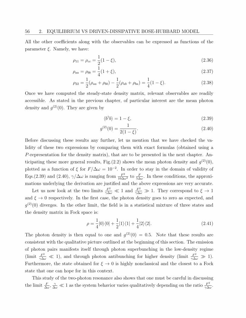
56 2. EQUILIBRIUM VS DRIVEN-DISSIPATIVE BOSE-HUBBARD MODEL
All the other coefficients along with the observables can be expressed as functions of theparameter ξ. Namely, we have:
ρ11 = ρcc =1
2(1− ξ), (2.36)
ρaa = ρbb =1
4(1 + ξ), (2.37)
ρ22 =1
2(ρaa + ρbb)−
1
2(ρab + ρba) =
1
4(1− ξ). (2.38)
Once we have computed the steady-state density matrix, relevant observables are readilyaccessible. As stated in the previous chapter, of particular interest are the mean photondensity and g(2)(0). They are given by
〈b†b〉 = 1− ξ, (2.39)
g(2)(0) =1
2(1− ξ) . (2.40)
Before discussing these results any further, let us mention that we have checked the va-lidity of these two expressions by comparing them with exact formulas (obtained using aP -representation for the density matrix), that are to be presented in the next chapter. An-ticipating these more general results, Fig.(2.2) shows the mean photon density and g(2)(0),plotted as a function of ξ for F/∆ω = 10−2. In order to stay in the domain of validity ofEqs.(2.39) and (2.40), γ/∆ω is ranging from F 2
10∆ω2 to F5∆ω
. In these conditions, the approxi-mations underlying the derivation are justified and the above expressions are very accurate.
Let us now look at the two limits F 2
γ∆ω 1 and F 2
γ∆ω 1. They correspond to ξ → 1
and ξ → 0 respectively. In the first case, the photon density goes to zero as expected, andg(2)(0) diverges. In the other limit, the field is in a statistical mixture of three states andthe density matrix in Fock space is:
ρ =1
4|0〉〈0|+ 1
2|1〉〈1|+ 1
4|2〉〈2|. (2.41)
The photon density is then equal to one and g(2)(0) = 0.5. Note that these results areconsistent with the qualitative picture outlined at the beginning of this section. The emissionof photon pairs manifests itself through photon superbunching in the low-density regime(limit F 2
γ∆ω 1), and through photon antibunching for higher density (limit F 2
γ∆ω 1).
Furthermore, the state obtained for ξ → 0 is highly nonclassical and the closest to a Fockstate that one can hope for in this context.
This study of the two-photon resonance also shows that one must be careful in discussingthe limit F
∆ω, γ
∆ω 1 as the system behavior varies qualitatively depending on the ratio F 2
γ∆ω.
Strongly Correlated Photons in Arrays of Nonlinear Cavities 57
0 0.5 1−0.01
−0.005
0
0.005
0.01
ξ
Re(<
b>
), Im
(<b
>)
0 0.5 10
0.5
1
1.5
2
ξ
ph
oto
n d
en
sity,
g2(0
)
Figure 2.2: Results for a single cavity. Left panel: real (continuous blue line) and imaginarypart (dotted-dashed red line), of the bosonic coherence 〈b〉 plotted vs ξ for F/∆ω = 10−2.The corresponding values of γ/∆ω range from F 2
10∆ω2 to F5∆ω
. Lines are the result of ex-act P -representation calculations while markers correspond to the simplified expression ofEq.(2.81). Right panel: mean photon density 〈b†b〉 (continuous blue line) and g(2)(0) (reddashed-dotted line), vs. ξ. Same conditions and conventions as in the other panel.
As one might expect, these results are not limited to n = 2. The next paragraph isdevoted to the general case with n > 2.
Generalized Fock states
In the case of n-photon resonance, the coupling between |0〉 and |n〉 is of the order n inF and the energy splitting proportional to F n/∆ωn−1. In what follows we show that a statesimilar to Eq.(2.41) may be obtained in the limit Fn
γ∆ωn−1 1.
The first thing to notice is that for n > 2, not only are the two states |0〉 and |n〉degenerate in the absence of driving, but it is also true for all the states |k〉, |q〉 withk + q = n. Instead of the two states |a〉 and |b〉 of Eq.(2.25), we have several pairs |ak〉,|bk〉 mixing |k〉 and |n− k〉. Before writing an explicit expression for the master equation inthe dressed basis, a few conclusions on the general structure of the equations can be drawnsolely from the fact that the Hamiltonian is diagonal in this basis.
In particular, generalizing Eqs.(2.30-2.33), we can write the master equation in the
58 2. EQUILIBRIUM VS DRIVEN-DISSIPATIVE BOSE-HUBBARD MODEL
dressed basis in the following way:
i∂tρjj = γ∑
pq
αjpqρpq, (2.42)
i∂tρij = (Ei − Ej)ρij + γ∑
pq
βijpqρpq, (2.43)
where i, j, p, q ∈ a1, b1, a2, b2 . . . ak, bk . . . , Ei,Ej are the energy levels of the rotating-frameHamiltonian and αjpq, βijpq are generic coefficients. From the second equation we concludethat coherences vanish in the steady-states. Indeed the smallest value for Ei − Ej is theenergy splitting between eigenstates inside the subspace |0〉, |n〉. As a consequence, in thelimit Fn
γ∆ωn−1 1, the difference Ei − Ej is always much larger than γ and the stationaryvalue for ρij goes to zero.
Taking this last result into account, the only stationary equations that remain to besolved contain only populations and may be written as:
∑
q
αjqqρqq = 0. (2.44)
Notice that in this expression, neither γ nor F appears explicitly.To go further we need to find the coefficients αjqq, which depend on the basis |ak〉, |bk〉.
In the following we show that the expression for the two-photon resonance can be readilyextended to the general case. Namely, the perturbed eigenstates, up to the lowest order inF , are:
|ak〉 =1√2
(|k〉+ |n− k〉), (2.45)
|bk〉 =1√2
(|k〉 − |n− k〉), (2.46)
for k integer and 0 ≤ k ≤ n/2.In its general formulation the problem of finding these eigenstates is solved by means
of time-independent perturbation theory with degenerate levels. To find energies, and thecorresponding eigenstates, one has to solve the so-called secular equation in each of thedegenerate subspaces [85]. More precisely, the energies are solutions of:
det[EP − heff (E)] = 0, (2.47)
where P is the projector onto the considered subspace and heff is the effective Hamiltonianinside the subspace, given by:
heff = PHP + PV QQ
EQ−HQQV P. (2.48)
Strongly Correlated Photons in Arrays of Nonlinear Cavities 59
Here we have introduced the projector Q = 1−P , and the perturbation operator V = F (b†+
b). We do not need to solve Eq.(2.47) completely to find the expression for the eigenstates.In particular, it is sufficient for our purpose to show that the effective Hamiltonian for eachsubspace has the form:
heff =
(D g
g D
). (2.49)
Indeed, such a matrix has eigenvectors similar to those of Eqs.(2.45)-(2.46).Since the unperturbed Hamiltonian has only real matrix elements and F is assumed to
be real, heff is a real matrix. It is also symmetric by definition. The only thing left to dois therefore to show that the two diagonal elements are equal. We are only interested in theleading terms in the expansion in powers F , which for the diagonal elements Dk and Dn−k
are of second order and given by [86]:
Dk =∑
n 6=k
|〈k|V |n〉|2
E(0)k − E
(0)n
=(k + 1)F 2
∆ω − kU +kF 2
−∆ω + (k − 1)U. (2.50)
Recalling the energy matching condition: U/∆ω = 2/(n− 1) we find:
Dk =−(n+ 1)F 2
∆ω(n− 2k − 1)(2k − n− 1), (2.51)
which satisfies the symmetry condition:
Dk = Dn−k, (2.52)
thereby showing that the effective Hamiltonian is of the form of Eq.(2.49). From this weconclude that the eigenstates of the full Hamiltonian, in the lowest order in F , are given byEq.(2.45) and Eq.(2.46).
The last step is to write an explicit equation for stationary populations in the basis|ak〉, |bk〉, . . . . For simplicity, we will assume that n is odd, so that there is no non-degenerate singlet, but the same reasoning is valid also for even values of n. Projecting themaster equation in the dressed basis and assuming that coherences vanish, we find:
nρakak −k + 1
2(ρak+1ak+1
+ ρbk+1bk+1)− n− k + 1
2(ρak−1ak−1
+ ρbk−1bk−1) = 0 (2.53)
nρbkbk −k + 1
2(ρak+1ak+1
+ ρbk+1bk+1)− n− k + 1
2(ρak−1ak−1
+ ρbk−1bk−1) = 0 (2.54)
60 2. EQUILIBRIUM VS DRIVEN-DISSIPATIVE BOSE-HUBBARD MODEL
In this form, these equations are valid from k = 0 to k = n−12−1. A last equation is provided
by the normalization condition Tr[ρ] = 1. We see that ak and bk play symmetric roles for allk. We have therefore:
ρakak = ρbkbk (2.55)
After this simplification, we are left with only one recurrence relation. The solution, up toa normalization constant, is provided by the binomial coefficients:
ρakak = ρbkbk =1
2nn!
k!(n− k)!=
1
2n
(n
k
). (2.56)
Since all non-diagonal coefficients of the density matrix vanish in the dressed basis, thepopulations in Fock space are given by:
〈k|ρ|k〉 =1
2(ρakak + ρbkbk) =
1
2n
(n
k
). (2.57)
Besides, it is clear that coherences between state |n〉 and |m〉 that do not belong to the samesubspace will vanish. As for coherences between |k〉 and |n− k〉, we have:
〈k|ρ|n− k〉 =1
2(ρakak − ρbkbk) = 0. (2.58)
Hence, the density matrix is also diagonal in Fock space.In conclusion, a state similar to Eq.(2.41) may be obtained in the limit Fn
γ∆ωn−1 1 andthe corresponding density matrix is:
ρ(n) =1
2n
n∑
k=0
(n
k
)|k〉〈k|. (2.59)
The state of Eq.(2.59) is characterized by:
〈b†b〉 =n
2, (2.60)
g(2)(0) = 1− 1
n. (2.61)
Note that the value of g(2)(0) is the same as in the nth-lobe of the equilibrium model (pureFock state with n photons). For this reason, we have called the mixed states of Eq.(2.59)“generalized Fock states”. From the point of view of photon statistics, these states are non-classical. However, their Wigner function has no negative part, as we will see in the following.Before getting into the details of Wigner function calculations, we emphasize that Eq.(2.59-2.61) also apply to n = 1 (∆ω = 0), in the limit F/U → 0 and γ/F → 0.
Strongly Correlated Photons in Arrays of Nonlinear Cavities 61
The Wigner transform is a way to map quantum mechanical Hermitian operators toreal functions in phase space. When applied to the density matrix it gives the Wignerfunction. This function is a quasi-probability distribution over phase space. The occurrenceof negative values is usually associated with “quantumness”. the Wigner function is definedas follows [87]:
W (β) =1
πTr[ρD(β)(−1)b
†bD(β)−1], (2.62)
where D(β) is the displacement operator, which transforms the vacuum state |0〉 into acoherent state |β〉:
D(β)|0〉 = e(βb†−β∗b)|0〉 = |β〉. (2.63)
Defined in this way, the Wigner function satisfies the normalization condition:∫W (β)d2β = 1. (2.64)
We see from Eq.(2.62) that the Wigner transform is linear in ρ. Since the density matrixρ(n) in Eq.(2.59) is a linear combination of pure Fock states, its Wigner function is a linearcombination of Fock states’ Wigner functions. The Wigner function of a Fock state with nphotons is given by [88]:
W (β) =2
π(−1)nLn(4|β|2)e−2|β|2 , (2.65)
with Ln(x) the nth Laguerre polynomial:
Ln(x) =n∑
k=0
(−1)k(n
k
)xk
k!. (2.66)
The Wigner function of ρ(n) is therefore of the form 2πe−2|β|2P (4|β|2), with P the polynomial:
P (x) =1
2n
n∑
k=0
k∑
q=0
(−1)k+q
(n
k
)(k
q
)xq
q!. (2.67)
Inverting the two summations and writing binomials coefficients explicitly we find:
P (x) =1
2n
n∑
q=0
(−1)qxq
q!
n∑
k=q
(−1)kn!
(n− k)!(k − q)!q! . (2.68)
This last expression can be simplified by rewriting the sum over k as a sum over k′ = n− k.The binomial coefficients
(nq
)and
(n−qk′
)naturally arise in the process and we get:
P (x) =1
2n
n∑
q=0
(−1)n+q
(n
q
)xq
q!
q∑
k′=0
(−1)k′(n− qk′
). (2.69)
62 2. EQUILIBRIUM VS DRIVEN-DISSIPATIVE BOSE-HUBBARD MODEL
The second sum, over k′, is non zero only if q = n. P (x) then reduces to a single monomialand its final expression is:
P (x) =xn
2nn!. (2.70)
The Wigner function for ρ(n) is then:
W (β) =2n+1|β|2nπn!
e−2|β|2 . (2.71)
Note that this function has its maximum for |β|2 = n/2, which is consistent with the factthat the mean photon number is n/2 in such a state. An interesting property of Eq.(2.71) isthat it is always positive. The effect of the statistical mixture is to suppress all the negativevalues present in each of the individual Fock states’ Wigner functions. Interestingly thesestates are quantum in terms of photon statistics (g(2)(0) < 1) but their Wigner functiondoes not take negative values. An example of Wigner function for pure and generalized Fockstates is shown on Fig.(2.3).
Driving out of multiphotonic resonances.
In the case where multiphotonic absorption processes are non resonant, the mean photonnumber is expected to be very low. In such conditions, the density matrix can be approxi-mated to lowest order in F/∆ω by a pure state [89]:
ρ = |ψ〉〈ψ|, (2.72)
with:
|ψ〉 =∑
n
cn|n〉. (2.73)
Both F/∆ω and γ/∆ω are assumed to be much smaller than one, but it is not necessary toimpose F γ. The following treatment is still valid if F/∆ω and γ/∆ω are of the sameorder of magnitude. Keeping the lowest order in F/∆ω and γ/∆ω for the coefficients cn, weobtain the following relation:
cn =F/∆ω
√ncn−1
n− n(n−1)2
U∆ω
+ inγ2∆ω
. (2.74)
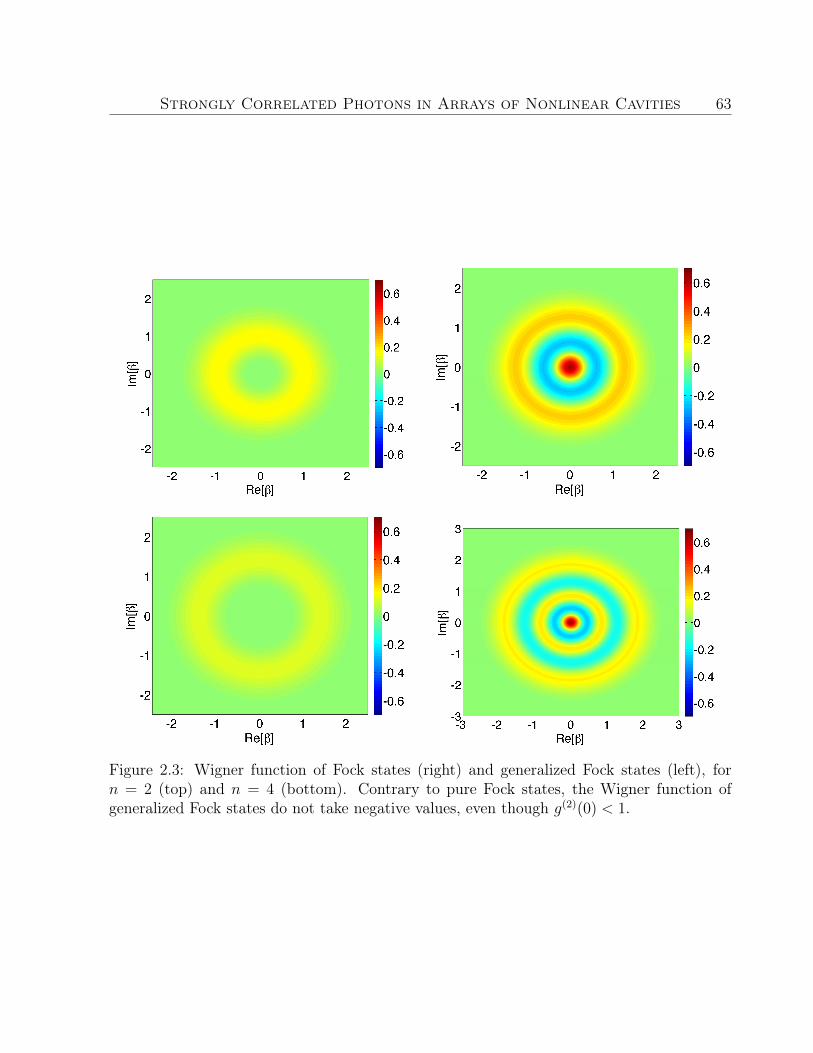
Strongly Correlated Photons in Arrays of Nonlinear Cavities 63
Figure 2.3: Wigner function of Fock states (right) and generalized Fock states (left), forn = 2 (top) and n = 4 (bottom). Contrary to pure Fock states, the Wigner function ofgeneralized Fock states do not take negative values, even though g(2)(0) < 1.
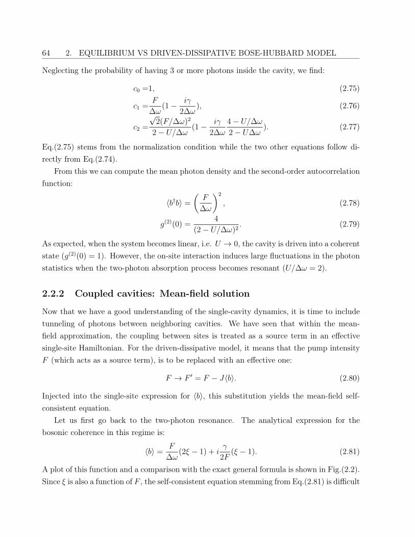
64 2. EQUILIBRIUM VS DRIVEN-DISSIPATIVE BOSE-HUBBARD MODEL
Neglecting the probability of having 3 or more photons inside the cavity, we find:
c0 =1, (2.75)
c1 =F
∆ω(1− iγ
2∆ω), (2.76)
c2 =
√2(F/∆ω)2
2− U/∆ω (1− iγ
2∆ω
4− U/∆ω2− U∆ω
). (2.77)
Eq.(2.75) stems from the normalization condition while the two other equations follow di-rectly from Eq.(2.74).
From this we can compute the mean photon density and the second-order autocorrelationfunction:
〈b†b〉 =
(F
∆ω
)2
, (2.78)
g(2)(0) =4
(2− U/∆ω)2. (2.79)
As expected, when the system becomes linear, i.e. U → 0, the cavity is driven into a coherentstate (g(2)(0) = 1). However, the on-site interaction induces large fluctuations in the photonstatistics when the two-photon absorption process becomes resonant (U/∆ω = 2).
2.2.2 Coupled cavities: Mean-field solution
Now that we have a good understanding of the single-cavity dynamics, it is time to includetunneling of photons between neighboring cavities. We have seen that within the mean-field approximation, the coupling between sites is treated as a source term in an effectivesingle-site Hamiltonian. For the driven-dissipative model, it means that the pump intensityF (which acts as a source term), is to be replaced with an effective one:
F → F ′ = F − J〈b〉. (2.80)
Injected into the single-site expression for 〈b〉, this substitution yields the mean-field self-consistent equation.
Let us first go back to the two-photon resonance. The analytical expression for thebosonic coherence in this regime is:
〈b〉 =F
∆ω(2ξ − 1) + i
γ
2F(ξ − 1). (2.81)
A plot of this function and a comparison with the exact general formula is shown in Fig.(2.2).Since ξ is also a function of F , the self-consistent equation stemming from Eq.(2.81) is difficult
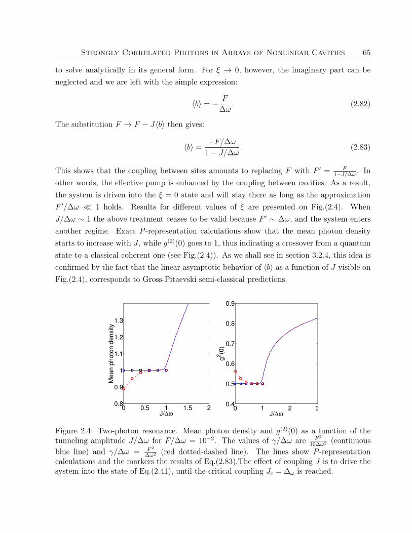
Strongly Correlated Photons in Arrays of Nonlinear Cavities 65
to solve analytically in its general form. For ξ → 0, however, the imaginary part can beneglected and we are left with the simple expression:
〈b〉 = − F
∆ω. (2.82)
The substitution F → F − J〈b〉 then gives:
〈b〉 =−F/∆ω
1− J/∆ω . (2.83)
This shows that the coupling between sites amounts to replacing F with F ′ = F1−J/∆ω . In
other words, the effective pump is enhanced by the coupling between cavities. As a result,the system is driven into the ξ = 0 state and will stay there as long as the approximationF ′/∆ω 1 holds. Results for different values of ξ are presented on Fig.(2.4). WhenJ/∆ω ∼ 1 the above treatment ceases to be valid because F ′ ∼ ∆ω, and the system entersanother regime. Exact P -representation calculations show that the mean photon densitystarts to increase with J , while g(2)(0) goes to 1, thus indicating a crossover from a quantumstate to a classical coherent one (see Fig.(2.4)). As we shall see in section 3.2.4, this idea isconfirmed by the fact that the linear asymptotic behavior of 〈b〉 as a function of J visible onFig.(2.4), corresponds to Gross-Pitaevski semi-classical predictions.
0 0.5 1 1.5 20.8
0.9
1
1.1
1.2
1.3
Mean p
hoto
n d
ensity
J/∆ω0 1 2 3
0.4
0.5
0.6
0.7
0.8
0.9
g2(0
)
J/∆ω
Figure 2.4: Two-photon resonance. Mean photon density and g(2)(0) as a function of thetunneling amplitude J/∆ω for F/∆ω = 10−2. The values of γ/∆ω are F 2
10∆ω2 (continuousblue line) and γ/∆ω = F 2
∆ω2 (red dotted-dashed line). The lines show P -representationcalculations and the markers the results of Eq.(2.83).The effect of coupling J is to drive thesystem into the state of Eq.(2.41), until the critical coupling Jc = ∆ω is reached.
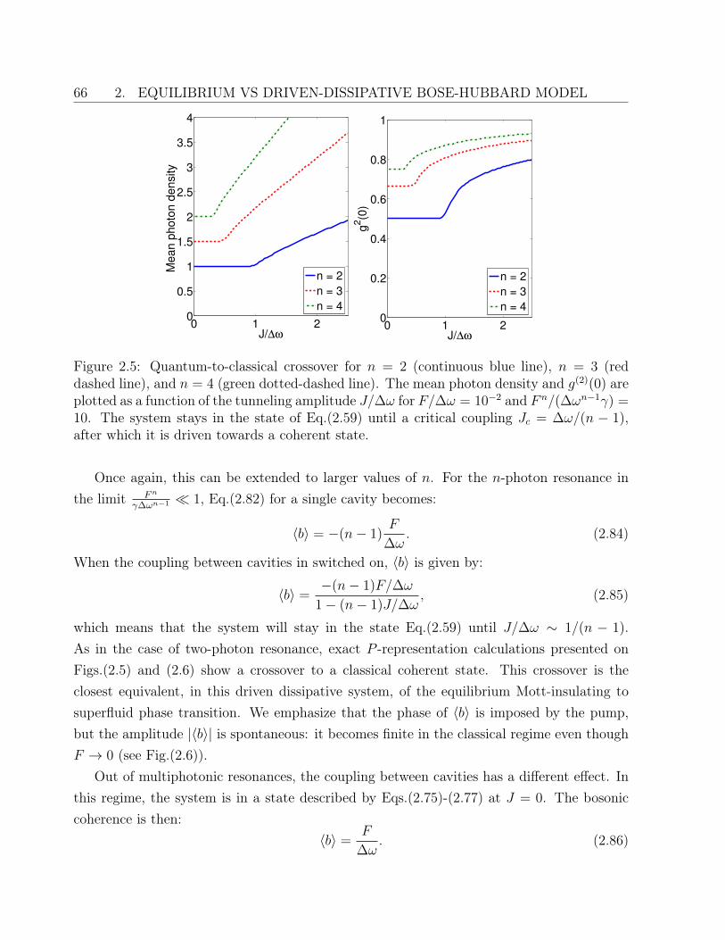
66 2. EQUILIBRIUM VS DRIVEN-DISSIPATIVE BOSE-HUBBARD MODEL
0 1 20
0.5
1
1.5
2
2.5
3
3.5
4
Mean p
hoto
n d
ensity
J/∆ω
n = 2
n = 3
n = 4
0 1 20
0.2
0.4
0.6
0.8
1
g2(0
)
J/∆ω
n = 2
n = 3
n = 4
Figure 2.5: Quantum-to-classical crossover for n = 2 (continuous blue line), n = 3 (reddashed line), and n = 4 (green dotted-dashed line). The mean photon density and g(2)(0) areplotted as a function of the tunneling amplitude J/∆ω for F/∆ω = 10−2 and F n/(∆ωn−1γ) =10. The system stays in the state of Eq.(2.59) until a critical coupling Jc = ∆ω/(n − 1),after which it is driven towards a coherent state.
Once again, this can be extended to larger values of n. For the n-photon resonance inthe limit Fn
γ∆ωn−1 1, Eq.(2.82) for a single cavity becomes:
〈b〉 = −(n− 1)F
∆ω. (2.84)
When the coupling between cavities in switched on, 〈b〉 is given by:
〈b〉 =−(n− 1)F/∆ω
1− (n− 1)J/∆ω, (2.85)
which means that the system will stay in the state Eq.(2.59) until J/∆ω ∼ 1/(n − 1).As in the case of two-photon resonance, exact P -representation calculations presented onFigs.(2.5) and (2.6) show a crossover to a classical coherent state. This crossover is theclosest equivalent, in this driven dissipative system, of the equilibrium Mott-insulating tosuperfluid phase transition. We emphasize that the phase of 〈b〉 is imposed by the pump,but the amplitude |〈b〉| is spontaneous: it becomes finite in the classical regime even thoughF → 0 (see Fig.(2.6)).
Out of multiphotonic resonances, the coupling between cavities has a different effect. Inthis regime, the system is in a state described by Eqs.(2.75)-(2.77) at J = 0. The bosoniccoherence is then:
〈b〉 =F
∆ω. (2.86)
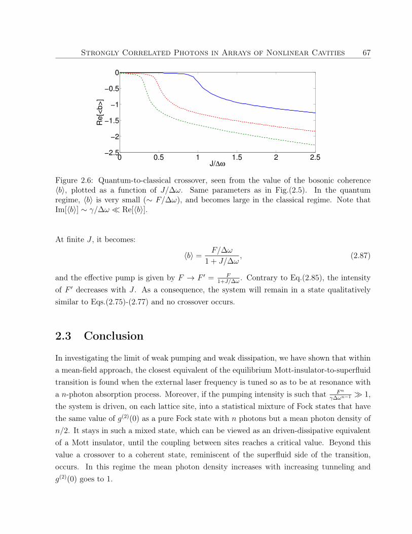
Strongly Correlated Photons in Arrays of Nonlinear Cavities 67
0 0.5 1 1.5 2 2.5−2.5
−2
−1.5
−1
−0.5
0
Re
[<b
>]
J/∆ω
Figure 2.6: Quantum-to-classical crossover, seen from the value of the bosonic coherence〈b〉, plotted as a function of J/∆ω. Same parameters as in Fig.(2.5). In the quantumregime, 〈b〉 is very small (∼ F/∆ω), and becomes large in the classical regime. Note thatIm[〈b〉] ∼ γ/∆ω Re[〈b〉].
At finite J , it becomes:
〈b〉 =F/∆ω
1 + J/∆ω, (2.87)
and the effective pump is given by F → F ′ = F1+J/∆ω
. Contrary to Eq.(2.85), the intensityof F ′ decreases with J . As a consequence, the system will remain in a state qualitativelysimilar to Eqs.(2.75)-(2.77) and no crossover occurs.
2.3 Conclusion
In investigating the limit of weak pumping and weak dissipation, we have shown that withina mean-field approach, the closest equivalent of the equilibrium Mott-insulator-to-superfluidtransition is found when the external laser frequency is tuned so as to be at resonance witha n-photon absorption process. Moreover, if the pumping intensity is such that Fn
γ∆ωn−1 1,the system is driven, on each lattice site, into a statistical mixture of Fock states that havethe same value of g(2)(0) as a pure Fock state with n photons but a mean photon density ofn/2. It stays in such a mixed state, which can be viewed as an driven-dissipative equivalentof a Mott insulator, until the coupling between sites reaches a critical value. Beyond thisvalue a crossover to a coherent state, reminiscent of the superfluid side of the transition,occurs. In this regime the mean photon density increases with increasing tunneling andg(2)(0) goes to 1.
68 2. EQUILIBRIUM VS DRIVEN-DISSIPATIVE BOSE-HUBBARD MODEL
Outside of these multiphotonic resonances, the mean-photon density is much smaller than1 and the state of the system is not as much affected by the coupling strength J , its effectbeing mainly to reduce the effective intensity of the pump. As a result, the photon statisticsis determined primely by the ratio U/∆ω. Photons are antibunched in the regime of photonblockade ( U/∆ω 1) but strongly bunched in the vicinity of the two-photon resonance(U/∆ω → 2).
These considerations encourage to distinguish between two types of steady-state phases.The first one is a “high-density phase”, with g(2)(0) ≤ 1 and a mean-photon density increasingwith the tunneling rate. The second one is a “low-density phase” with 〈b†b〉 1 and possiblylarge fluctuations in the photon statistics. We will see in the next chapter that these generalcharacteristics of the steady-states remain visible at higher pumping and dissipation.
Chapter 3
Mean-field phase diagram of thedriven-dissipative Bose-Hubbard model
In the previous chapter, we addressed the issue of driving and dissipation by solving themaster equation in the Fock basis or in a dressed basis with only a few photons per site.This approach, which enabled us to derive analytical expressions for the single-site and mean-field density matrix, is well suited for weak pumping, when the mean number of photonsinside the cavity is small. It is not efficient however, if a large number of Fock states percavity must be taken into account. In this chapter, we will consider another method basedon a coherent-state representation of the density matrix, which turns out to be much morepowerful.
We begin by a few general considerations on how to use the coherent-state basis to rep-resent operators and density matrices. Building up on the relative freedom in the choice ofa representation given by the overcompleteness of the basis, we introduce a series of repre-sentations, known as “generalized P-representations”. We will see that the main advantageof these representations is that they provide a way to map the operatorial master equationinto the better-known Fokker-Planck equation. As shown by Drummond and Walls [90],generalized P-representations provide a general solution to the problem of a single nonlinearcavity.
By applying this exact result to mean-field theory, we are able to compute the phasediagram in the general case of arbitrary pumping and dissipation. One of the importantfeatures of the mean-field phase diagram is the appearance of bistability induced by thecoupling between the cavities. For some values of the tunneling coefficient, several solutionsof the self-consistent mean-field equation are found. We will see that many of the resultsobtained in the previous chapter, in particular those regarding the role of multiphotonic
69
70 3. MEAN-FIELD PHASE DIAGRAM
resonances, are still relevant for the understanding of the steady-state phases at higherpumping and dissipation.
We then go further in our investigation of the phase diagram by studying the stability ofthe different solutions and their collective excitations. We compute the dispersion relationby linearizing the master equation around the mean-field steady state. This “generalizedBogoliubov approach” enables us to identify tunneling-induced instabilities in the phasediagram, signaling the breaking of translational symmetry in the lattice. Indeed, in certainregions of the parameter space, no stable homogeneous mean-field solutions have been found.
Throughout the chapter, P -representation calculations are compared with results ob-tained using a Gross-Pitaevskii (semi-classical) approach.
For the most part, the work presented in this chapter has been published in Ref.[23]. Thecomparison with the Gross-Pitaevskii approximation is included in Ref.[22].
Strongly Correlated Photons in Arrays of Nonlinear Cavities 71
3.1 Phase-space approach to quantum optics
Given the role that they play in the theoretical formulation of quantum optics, the set ofcoherent states seems a natural alternative to the Fock basis. As seen in Chap.1, theirexpression in Fock space is:
|α〉 = e−|α|2/2
∞∑
n=0
αn√n!|n〉. (3.1)
3.1.1 Coherent-state representation of the density matrix
The general problem of finding an expression for the density matrix in terms of coherent-state projection operators may be formulated in the following way: find a function F(α, β)
and an appropriate domain D ⊂ C2 such that
ρ =
∫ ∫
DF(α, β)|α〉〈β∗|d2αd2β. (3.2)
If the basis were not overcomplete, such a function F(α, β) would be unique and equal tothe matrix elements of ρ in this basis: 〈α|ρ|β∗〉. Besides, the integral would run over thewhole space C2. However, as we have seen, coherent states are not orthogonal and thus theproblem of finding F(α, β),D is not trivial. A consequence of the basis’ overcompletnessis that the set of all matrix elements 〈α|ρ|β∗〉 contains a lot of redundant information. Infact, it can be shown that, in this basis, the density matrix is already entirely determinedby its diagonal elements. To see this more clearly, let us write those matrix elements as
〈α|ρ|α〉 =∑
n,m
〈n|ρ|m〉e−|α|2 (α∗)n(α)m√n!m!
. (3.3)
We deduce from this expression that eαα∗〈α|ρ|α〉 acts as a kind of generating series for thematrix elements in Fock space. We find therefore:
〈n|ρ|m〉 =1√n!m!
∂n
∂α∗n∂m
∂αm(eαα
∗〈α|ρ|α〉)∣∣∣α=0
. (3.4)
Coming back to the task of finding F(α, β),D, this last result suggests to look for arepresentation based only on diagonal projection operators:
ρ =
∫PGS(α, α∗)|α〉〈α|d2α. (3.5)
This is the Glauber-Sudarshan P -representation, introduced by Glauber and Sudarshan [91,92]. It was shown to exist for all density operators but is not necessarily regular. In general
72 3. MEAN-FIELD PHASE DIAGRAM
it is expressed in terms of singular distributions such as successive derivatives of the Diracdistribution [88]. An example of such singular P function is given by the coherent statesthemselves, since the P representation of a coherent state |α0〉 is:
PGS(α, α∗) = δ(α− α0). (3.6)
At this point, it is important to keep in mind that the ultimate aim is for the representationof ρ to provide a efficient “encoding” of the system’s dynamics. More precisely, in the sameway that, projected into Fock space, the master equation yields a set of differential equationsfor the matrix elements in this basis, the same master equation will result in an equation ofmotion for the function F(α, β). In this regard, the singularity of the Glauber-Sudarshanrepresentation appears as an important drawback.
Although it may seem more “economical” in terms of information to work only withdiagonal matrix elements, it is not the only alternative. In order to make the best of therelative freedom in the choice of the function F , Drummond and Gardiner have proposed amore systematic scheme of defining representations by expanding ρ in terms of nondiagonalcoherent-state projection operators [93]. Their “generalized P -representations” are of theform:
ρ =
∫P (α, β)Λ(α, β)dµ(α, β), (3.7)
where Λ(α, β) is a projection operator:
Λ(α, β) =|α〉〈β∗|〈β∗|α〉 , (3.8)
and dµ(αβ) the integration measure, whose choice will determine the different types ofrepresentation. As a first example, let us consider:
dµ(α, β) = δ(α− β∗)d2αd2β. (3.9)
We recover in this case the Glauber-Sudarshan P -representation defined in Eq.(3.5).
Complex P-representation
The complex P -representation is defined by
dµ(α, β) = dαdβ, (3.10)
Strongly Correlated Photons in Arrays of Nonlinear Cavities 73
where α and β are two complex variables that are to be integrated on individual contoursCα and Cβ. In such a representation, ρ is therefore written as:
ρ =
∫
Cβ
∫
CαP (α, β)
|α〉〈β∗|〈β∗|α〉 dαdβ. (3.11)
Positive P-representation
Another useful representation is obtained for:
dµ = d2αd2β, (3.12)
allowing α and β to vary over the whole complex plane. One of the advantages of thisrepresentation is that it can always be chosen positive and thus be interpreted as a genuineprobability distribution over a complex phase space (α, β). More precisely, it can be shownthat its relation to matrix elements of ρ is [88]:
P (α, β) =1
4π2e−|α−β|2
4 〈12
(α + β∗)|ρ|12
(α + β∗)〉, (3.13)
which constitutes another proof that a density operator is entirely determined by coherentstates diagonal matrix elements.
3.1.2 Fokker-Planck equations for generalized P -representations
One of the most interesting features of these coherent-state representations is that when thedynamics is described by the usual quantum optical master equation, the equation of motionobtained for P (α, β) takes the form of a Fokker-Planck equation. In this respect, the useof coherent-state representation has often been seen as establishing a quantum-to-classicalcorrespondence, in the sense that the quantum master equation is mapped to the classicalproblem of diffusion in phase space. Note however that depending on the Hamiltonian, thisequation may contain terms of higher order than the usual Fokker-Planck equation and maynot be exactly solvable. The choice of representation is in fact dictated by the specific formof the resulting equation. For each of the representations, it is possible to build a “translationtable” which indicates how to convert operators acting on ρ to differential operators actingon P (α, β).
Details of the derivation will be given only for the complex P -representation, since it willbe the only one needed to solve the single cavity problem, but the procedure is essentially
74 3. MEAN-FIELD PHASE DIAGRAM
the same for the other representations. The first step is to find the action of the creation andannihilation operators on the projectors Λ(α, β). It is most easily done by using unnormalizedcoherent states (also known as Bargmann states):
||β〉 =∞∑
n=0
βn√n!|n〉 = e|β|
2/2|β〉, (3.14)
which have the following nice properties:
b||β〉 = β||β〉, (3.15)
b†||β〉 =∂
∂β||β〉. (3.16)
Expressed in terms of this new states, the projectors Λ(α, β) read:
Λ(α, β) = e−αβ||α〉〈β∗||, (3.17)
from which we deduce:
bΛ(α, β) = αΛ(α, β), (3.18)
b†Λ(α, β) = (∂
∂α+ β)Λ(α, β), (3.19)
Λ(α, β)b† = βΛ(α, β), (3.20)
Λ(α, β)b = (∂
∂β+ α)Λ(α, β). (3.21)
Injecting these last results into Eq.(3.11):
bρ =
∫
Cβ
∫
CαP (α, β)αΛ(α, β)dαdβ, (3.22)
b†ρ =
∫
Cβ
∫
CαP (α, β)(
∂
∂α+ β)Λ(α, β)dαdβ, (3.23)
ρb† =
∫
Cβ
∫
CαP (α, β)βΛ(α, β)dαdβ, (3.24)
ρb =
∫
Cβ
∫
CαP (α, β)(
∂
∂β+ α)Λ(α, β)dαdβ. (3.25)
The differential operators acting on Λ generate operations on P (α, β) by integration by part.The integration contours have then to be chosen such that the boundary terms vanish, which
Strongly Correlated Photons in Arrays of Nonlinear Cavities 75
is always possible [93]. Finally we arrive at the following “translation table”:
bρ→ αP (α, β), (3.26)
b†ρ→ (− ∂
∂α+ β)P (α, β), (3.27)
ρb† → βP (α, β), (3.28)
ρb→ (− ∂
∂β+ α)P (α, β). (3.29)
From this we see that quadratic terms in the Hamiltonian will generate first order deriva-tives whereas second order derivatives will arise from quartic terms such as photon-photoninteraction. Hence, the master equation takes the form of a Fokker-Planck equation on P :
∂tP (α) =
(∂
∂αiAi(α) +
1
2
∂
∂αi
∂
∂αjDij(α)
)P (α), (3.30)
where we have used the short-hand notation α = (α1, α2) = (α, β). The general form ofthis equation remains the same for all P representations, but for a given representation, thediffusion matrix D is not always positive definite.
Before going into the details of the implementation of Eq.(3.30) in the case of the singlenonlinear cavity, let us mention, for the sake of generality, two other phase-space functions.One is the Wigner function that we have already encountered in the preceding chapter, theother is the Q-function or Husimi function.
3.1.3 Husimi and Wigner functions
In defining the P -representation, we associated a function of complex variables to the densitymatrix by imposing the form of the decomposition of ρ, while the expression for P remainedimplicit in the definition. What then needed to be proved was the existence of such function.It is also possible to proceed in another way, by first, giving an explicit expression for thefunction and second, verify that all the properties of the operator ρ can be recovered fromthis function. Both Wigner and Husimi functions are defined this way.
Husimi function
The Husimi or Q-function is defined as follows [94]:
Q(α, α∗) =1
π〈α|ρ|α〉. (3.31)
76 3. MEAN-FIELD PHASE DIAGRAM
Since ρ is Hermitian, Q(α, α∗) is positive. Besides, the factor 1/π ensure that it is normalizedto unity: using the resolution of identity for coherent states we find
∫Q(α, α∗)d2α = 1. (3.32)
Therefore this function behaves like a probability distribution. It is well suited for calculationof averages of antinormally ordered operators:
Tr(ρbnb†m) =
∫αnα∗mQ(α, α∗)d2α. (3.33)
It is interesting to note that the density matrix in Fock space can be reconstructed fromthe Q-function, showing that all the properties of the field are contained in this function.The first step in the derivation is to show that the Q-function may be expressed as a powerseries in α and α∗ [88]:
Q(α, α∗) =∑
n,m
Qn,mαmα∗n, (3.34)
with
Qn,m = e−αα∗ 〈n|ρ|m〉π√n!m!
. (3.35)
Then, the matrix elements of the density operator are given by:
〈n|ρ|m〉 = π√n!m!
∑
r
Qn−r,m−r. (3.36)
Wigner function
Since we have already encountered the Wigner function in chapter 2 (see the definitionin Eq.(2.62)), we will just briefly add that this quasiprobability distribution is useful forcomputing symmetrically ordered products of creation and annihilation operators:
〈bnb†msym.〉 =
∫αnα∗mW (α, α∗)dα. (3.37)
We have seen that, in contrast with the Husimi function, the Wigner function may takenegative values. A Wigner function with negative value indicates that the state of theelectromagnetic field under consideration cannot be understood within a purely classicaltheory.
Strongly Correlated Photons in Arrays of Nonlinear Cavities 77
3.1.4 Exact solution of the single-cavity problem
The phase-space approach was successfully applied by Drummond and Walls to the problemof a single nonlinear cavity [90]. Using a complex P-representation for the density matrix,they were able to solve the corresponding Fokker-Planck equation and compute exactly allone-time correlation functions in the steady-state. The details of the derivation are presentedin Ref.[90], we only give here the final result:
〈(b†)j(b)j〉 =
∣∣∣∣2F
U
∣∣∣∣2j
× Γ(c)Γ(c∗)
Γ(c+ j)Γ(c∗ + j)
× F(j + c, j + c∗, 8|F/U |2)
F(c, c∗, 8|F/U |2), (3.38)
with
c = 2(−∆ω − iγ/2)/U, (3.39)
and the hypergeometric function
F(c, d, z) =∞∑
n
Γ(c)Γ(d)
Γ(c+ n)Γ(d+ n)
zn
n!, (3.40)
where Γ is the gamma special function.The coefficients of the density matrix can be computed in a similar way:
ρp,q =1√p!q!
(−2F
U
)p(−2F ∗
U
)qΓ(c)Γ(c∗)
Γ(c+ p)Γ(c∗ + q)
F(c+ p, c∗ + q, 4|F/U |2)
F(c, c∗, 8|F/U |2), (3.41)
As an illustration of the usefulness of these formulas, let us rederive in a much quicker andmore elegant manner the expression of the generalized Fock states found in Eq.(2.59), in thelimit γ F ∆ω.
In correspondence of a n-photon resonance, with n > 1, the constant c in Eq.(3.39) isgiven by
c = −(n− 1)(1 + iγ
2∆ω), (3.42)
which means that c ≈ −(n − 1) for γ ∆ω. Since the gamma function has poles at zeroand negative integer values, the quantities Γ(c + k),Γ(c∗ + k) are diverging for 0 ≤ k < n,implying that certain coefficients of the hypergeometric series (3.40) will actually diverge inthe limit γ F ∆ω.
78 3. MEAN-FIELD PHASE DIAGRAM
From the above consideration, the leading contribution in the two hypergeometric func-tions in Eq.(3.41) are given by
F(c, c∗, 2z) ' Γ(c)Γ(c∗)
Γ(c+ n)Γ(c∗ + n)
(2z)n
n!, (3.43)
and
F(c+ k, c∗ + k, z) ' Γ(c+ k)Γ(c∗ + k)
Γ(c+ n)Γ(c∗ + n)
zn−k
(n− k)!, (3.44)
respectively, where z = 4F 2/U2.Substituting Eqs.(3.43) and (3.44) into the general expression for the density matrix,
Eq.(3.41), we find
ρkk =1
2nk!
n
(n− k)!, (3.45)
which corresponds exactly to Eq.(2.59).It is also easy to see that off-diagonal terms will instead vanish in the same limit γ
F ∆ω. Indeed, a similar analysis gives for q < p (the opposite case can be treated in thesame way):
ρpq =1√p!q!
(−2F
U
)p−q1
2nn!
(n− q)!(p− q)! , (3.46)
which indeed vanishes for vanishing pump amplitude, F → 0.The expression for the bosonic coherence is obtained in a similar way. The general formula
for 〈b〉 is:
〈b〉 =F
∆ω + iγ/2× F(1 + c, c∗, 8|F
U|2)
F(c, c∗, 8|FU|2)
, (3.47)
and the leading term in the geometric function appearing in the numerator is:
F(c+ 1, c∗, 2z) ' Γ(c+ 1)Γ(c∗)
Γ(c+ 1 + n)Γ(c∗ + n)
(2z)n
n!. (3.48)
Using Eq.(3.43), we recover the result of Eq.(2.82):
〈b〉 = −(n− 1)F
∆ω. (3.49)
Apart from this new derivation, the exact formulas are of course a powerful tool for computingthe mean-field phase diagram of the model in the general case, for arbitrary pumping anddissipation.
Strongly Correlated Photons in Arrays of Nonlinear Cavities 79
3.2 Tunneling-induced bistability
The results for the single cavity can be directly applied to mean-field theory by performingthe substitution F → F ′ = F −J〈b〉 of Eq.(2.80) and solving the self-consistent equation for〈b〉 stemming from Eq.(3.47):
〈b〉 =(F − J〈b〉)∆ω + iγ/2
× F(1 + c, c∗, 8|F−J〈b〉U|2)
F(c, c∗, 8|F−J〈b〉U|2)
. (3.50)
The complete phase diagram can be extracted from Eq.(3.50) by solving the equation nu-merically. It is most easily done by starting from the exact result at J = 0 and increasing thetunneling strength step by step, taking the solution at step n as the initial value (requiredby the numerical solver), of the step n+ 1.
One of the key features of the mean-field phase diagram turned out to be “tunneling-induced” bistability. That is, due to the substitution F → F − J〈b〉 performed when con-sidering coupled cavities, the Eq.(3.50) may have multiple solutions, giving rise to severalsteady-states phases (for the same values of all the parameters). The remainder of this sec-tion will be devoted to getting a clearer understanding of this phenomenon. However, beforelooking at the most general case, it is useful to stay in the limit of weak dissipation whileallowing the pump intensity to take arbitrary values. This regime has the virtue of eliminat-ing one variable in an already large enough parameter space. Besides, upon “elimination” ofγ, the functions involved in Eq.(3.50) become real (providing the field F is assumed to bereal as well). It is therefore possible to visualize the solutions of the self-consistent equationgraphically.
3.2.1 Solution for arbitrary pumping and weak dissipation
Interestingly, it turns out that for arbitrary pumping intensity, correlation functions calcu-lated via the exact formula of Eq.(3.38) have a finite limit for γ → 0. As in the previouschapter a good starting point is the isolated cavity.
Isolated Cavity
We know from Chap. 2 that in the limit of weak dissipation, if the intensity of the pumpis also weak, the effect of multiphotonic resonances plays an important role. In particular,the resonances are visible in the form of peaks in the mean photon density when plotted as
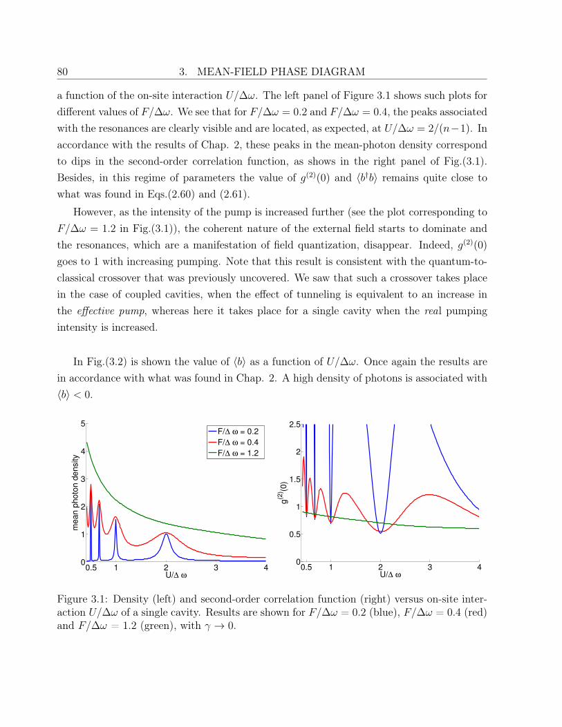
80 3. MEAN-FIELD PHASE DIAGRAM
a function of the on-site interaction U/∆ω. The left panel of Figure 3.1 shows such plots fordifferent values of F/∆ω. We see that for F/∆ω = 0.2 and F/∆ω = 0.4, the peaks associatedwith the resonances are clearly visible and are located, as expected, at U/∆ω = 2/(n−1). Inaccordance with the results of Chap. 2, these peaks in the mean-photon density correspondto dips in the second-order correlation function, as shows in the right panel of Fig.(3.1).Besides, in this regime of parameters the value of g(2)(0) and 〈b†b〉 remains quite close towhat was found in Eqs.(2.60) and (2.61).
However, as the intensity of the pump is increased further (see the plot corresponding toF/∆ω = 1.2 in Fig.(3.1)), the coherent nature of the external field starts to dominate andthe resonances, which are a manifestation of field quantization, disappear. Indeed, g(2)(0)
goes to 1 with increasing pumping. Note that this result is consistent with the quantum-to-classical crossover that was previously uncovered. We saw that such a crossover takes placein the case of coupled cavities, when the effect of tunneling is equivalent to an increase inthe effective pump, whereas here it takes place for a single cavity when the real pumpingintensity is increased.
In Fig.(3.2) is shown the value of 〈b〉 as a function of U/∆ω. Once again the results arein accordance with what was found in Chap. 2. A high density of photons is associated with〈b〉 < 0.
0.5 1 2 3 40
1
2
3
4
5
me
an
ph
oto
n d
en
sity
U/∆ ω
F/∆ ω = 0.2
F/∆ ω = 0.4
F/∆ ω = 1.2
0.5 1 2 3 40
0.5
1
1.5
2
2.5
g(2
) (0)
U/∆ ω
Figure 3.1: Density (left) and second-order correlation function (right) versus on-site inter-action U/∆ω of a single cavity. Results are shown for F/∆ω = 0.2 (blue), F/∆ω = 0.4 (red)and F/∆ω = 1.2 (green), with γ → 0.
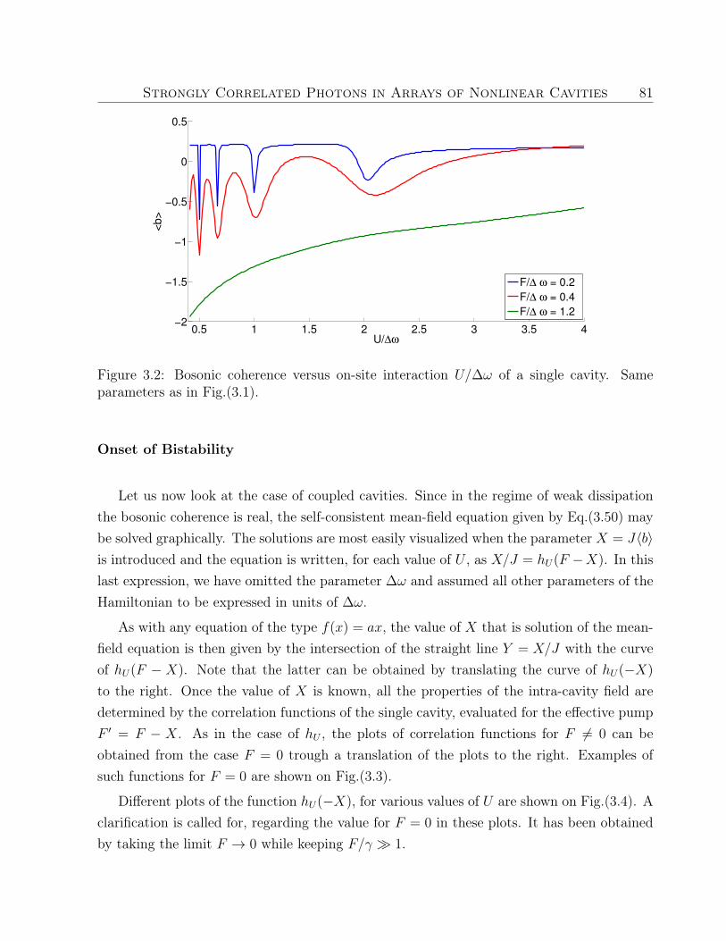
Strongly Correlated Photons in Arrays of Nonlinear Cavities 81
0.5 1 1.5 2 2.5 3 3.5 4−2
−1.5
−1
−0.5
0
0.5
<b
>
U/∆ω
F/∆ ω = 0.2
F/∆ ω = 0.4
F/∆ ω = 1.2
Figure 3.2: Bosonic coherence versus on-site interaction U/∆ω of a single cavity. Sameparameters as in Fig.(3.1).
Onset of Bistability
Let us now look at the case of coupled cavities. Since in the regime of weak dissipationthe bosonic coherence is real, the self-consistent mean-field equation given by Eq.(3.50) maybe solved graphically. The solutions are most easily visualized when the parameter X = J〈b〉is introduced and the equation is written, for each value of U , as X/J = hU(F −X). In thislast expression, we have omitted the parameter ∆ω and assumed all other parameters of theHamiltonian to be expressed in units of ∆ω.
As with any equation of the type f(x) = ax, the value of X that is solution of the mean-field equation is then given by the intersection of the straight line Y = X/J with the curveof hU(F − X). Note that the latter can be obtained by translating the curve of hU(−X)
to the right. Once the value of X is known, all the properties of the intra-cavity field aredetermined by the correlation functions of the single cavity, evaluated for the effective pumpF ′ = F − X. As in the case of hU , the plots of correlation functions for F 6= 0 can beobtained from the case F = 0 trough a translation of the plots to the right. Examples ofsuch functions for F = 0 are shown on Fig.(3.3).
Different plots of the function hU(−X), for various values of U are shown on Fig.(3.4). Aclarification is called for, regarding the value for F = 0 in these plots. It has been obtainedby taking the limit F → 0 while keeping F/γ 1.
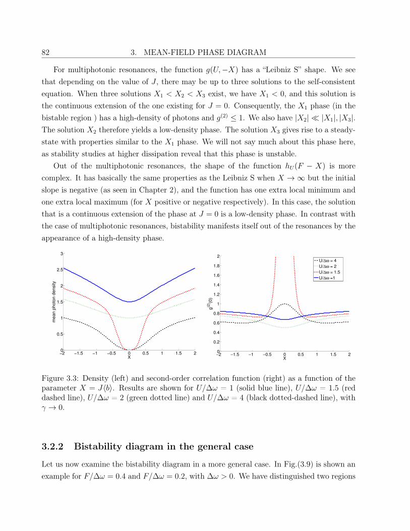
82 3. MEAN-FIELD PHASE DIAGRAM
For multiphotonic resonances, the function g(U,−X) has a “Leibniz S” shape. We seethat depending on the value of J , there may be up to three solutions to the self-consistentequation. When three solutions X1 < X2 < X3 exist, we have X1 < 0, and this solution isthe continuous extension of the one existing for J = 0. Consequently, the X1 phase (in thebistable region ) has a high-density of photons and g(2) ≤ 1. We also have |X2| |X1|, |X3|.The solution X2 therefore yields a low-density phase. The solution X3 gives rise to a steady-state with properties similar to the X1 phase. We will not say much about this phase here,as stability studies at higher dissipation reveal that this phase is unstable.
Out of the multiphotonic resonances, the shape of the function hU(F − X) is morecomplex. It has basically the same properties as the Leibniz S when X →∞ but the initialslope is negative (as seen in Chapter 2), and the function has one extra local minimum andone extra local maximum (for X positive or negative respectively). In this case, the solutionthat is a continuous extension of the phase at J = 0 is a low-density phase. In contrast withthe case of multiphotonic resonances, bistability manifests itself out of the resonances by theappearance of a high-density phase.
−2 −1.5 −1 −0.5 0 0.5 1 1.5 20
0.5
1
1.5
2
2.5
3
mean p
hoto
n d
ensity
X
−2 −1.5 −1 −0.5 0 0.5 1 1.5 20
0.2
0.4
0.6
0.8
1
1.2
1.4
1.6
1.8
2
g(2
) (0)
X
U/∆ω = 4
U/∆ω = 2
U/∆ω = 1.5
U/∆ω =1
Figure 3.3: Density (left) and second-order correlation function (right) as a function of theparameter X = J〈b〉. Results are shown for U/∆ω = 1 (solid blue line), U/∆ω = 1.5 (reddashed line), U/∆ω = 2 (green dotted line) and U/∆ω = 4 (black dotted-dashed line), withγ → 0.
3.2.2 Bistability diagram in the general case
Let us now examine the bistability diagram in a more general case. In Fig.(3.9) is shown anexample for F/∆ω = 0.4 and F/∆ω = 0.2, with ∆ω > 0. We have distinguished two regions
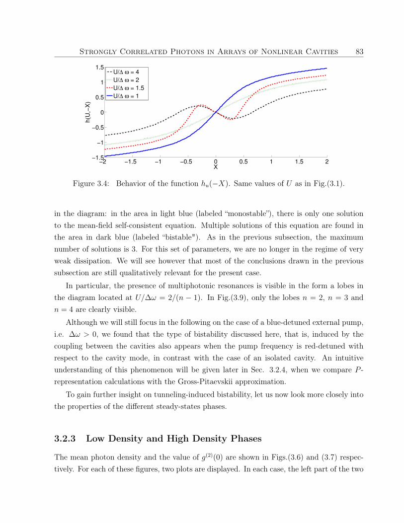
Strongly Correlated Photons in Arrays of Nonlinear Cavities 83
−2 −1.5 −1 −0.5 0 0.5 1 1.5 2−1.5
−1
−0.5
0
0.5
1
1.5
h(U
,−X
)
X
U/∆ ω = 4
U/∆ ω = 2
U/∆ ω = 1.5
U/∆ ω = 1
Figure 3.4: Behavior of the function hu(−X). Same values of U as in Fig.(3.1).
in the diagram: in the area in light blue (labeled “monostable”), there is only one solutionto the mean-field self-consistent equation. Multiple solutions of this equation are found inthe area in dark blue (labeled “bistable"). As in the previous subsection, the maximumnumber of solutions is 3. For this set of parameters, we are no longer in the regime of veryweak dissipation. We will see however that most of the conclusions drawn in the previoussubsection are still qualitatively relevant for the present case.
In particular, the presence of multiphotonic resonances is visible in the form a lobes inthe diagram located at U/∆ω = 2/(n − 1). In Fig.(3.9), only the lobes n = 2, n = 3 andn = 4 are clearly visible.
Although we will still focus in the following on the case of a blue-detuned external pump,i.e. ∆ω > 0, we found that the type of bistability discussed here, that is, induced by thecoupling between the cavities also appears when the pump frequency is red-detuned withrespect to the cavity mode, in contrast with the case of an isolated cavity. An intuitiveunderstanding of this phenomenon will be given later in Sec. 3.2.4, when we compare P -representation calculations with the Gross-Pitaevskii approximation.
To gain further insight on tunneling-induced bistability, let us now look more closely intothe properties of the different steady-states phases.
3.2.3 Low Density and High Density Phases
The mean photon density and the value of g(2)(0) are shown in Figs.(3.6) and (3.7) respec-tively. For each of these figures, two plots are displayed. In each case, the left part of the two
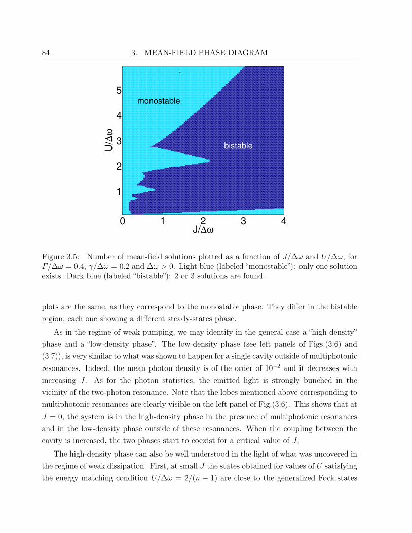
84 3. MEAN-FIELD PHASE DIAGRAM
0 1 2 3 4
1
2
3
4
5
J/∆ω
U/∆
ω
bistable
monostable
Figure 3.5: Number of mean-field solutions plotted as a function of J/∆ω and U/∆ω, forF/∆ω = 0.4, γ/∆ω = 0.2 and ∆ω > 0. Light blue (labeled “monostable”): only one solutionexists. Dark blue (labeled “bistable”): 2 or 3 solutions are found.
plots are the same, as they correspond to the monostable phase. They differ in the bistableregion, each one showing a different steady-states phase.
As in the regime of weak pumping, we may identify in the general case a “high-density”phase and a “low-density phase”. The low-density phase (see left panels of Figs.(3.6) and(3.7)), is very similar to what was shown to happen for a single cavity outside of multiphotonicresonances. Indeed, the mean photon density is of the order of 10−2 and it decreases withincreasing J . As for the photon statistics, the emitted light is strongly bunched in thevicinity of the two-photon resonance. Note that the lobes mentioned above corresponding tomultiphotonic resonances are clearly visible on the left panel of Fig.(3.6). This shows that atJ = 0, the system is in the high-density phase in the presence of multiphotonic resonancesand in the low-density phase outside of these resonances. When the coupling between thecavity is increased, the two phases start to coexist for a critical value of J .
The high-density phase can also be well understood in the light of what was uncovered inthe regime of weak dissipation. First, at small J the states obtained for values of U satisfyingthe energy matching condition U/∆ω = 2/(n − 1) are close to the generalized Fock states
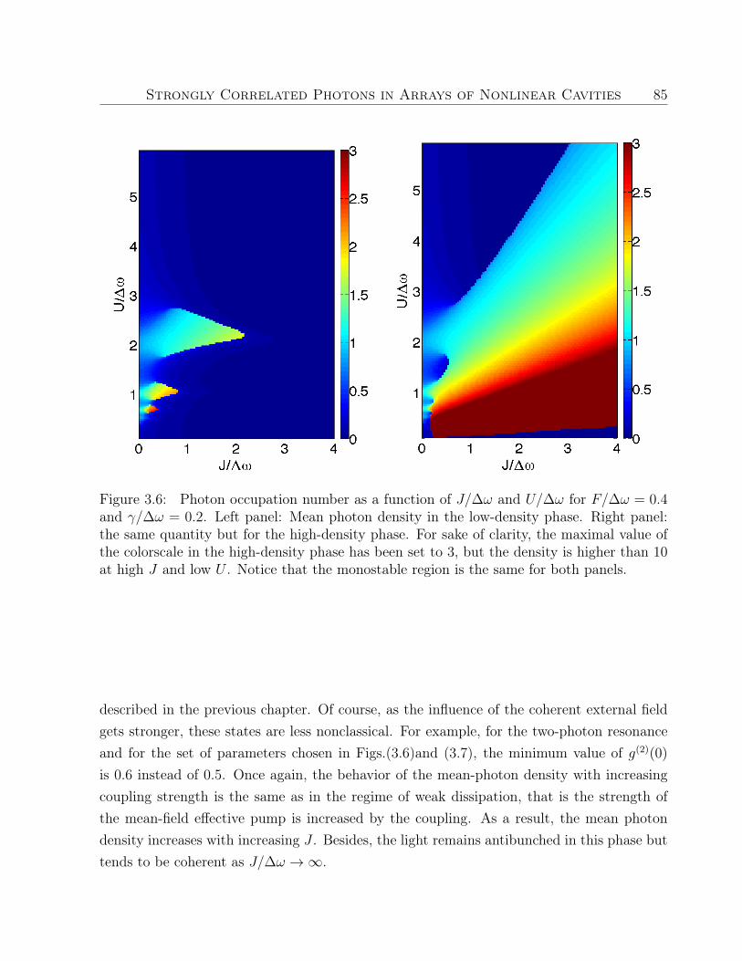
Strongly Correlated Photons in Arrays of Nonlinear Cavities 85
Figure 3.6: Photon occupation number as a function of J/∆ω and U/∆ω for F/∆ω = 0.4and γ/∆ω = 0.2. Left panel: Mean photon density in the low-density phase. Right panel:the same quantity but for the high-density phase. For sake of clarity, the maximal value ofthe colorscale in the high-density phase has been set to 3, but the density is higher than 10at high J and low U . Notice that the monostable region is the same for both panels.
described in the previous chapter. Of course, as the influence of the coherent external fieldgets stronger, these states are less nonclassical. For example, for the two-photon resonanceand for the set of parameters chosen in Figs.(3.6)and (3.7), the minimum value of g(2)(0)
is 0.6 instead of 0.5. Once again, the behavior of the mean-photon density with increasingcoupling strength is the same as in the regime of weak dissipation, that is the strength ofthe mean-field effective pump is increased by the coupling. As a result, the mean photondensity increases with increasing J . Besides, the light remains antibunched in this phase buttends to be coherent as J/∆ω →∞.
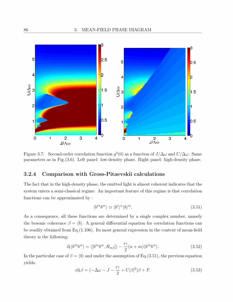
86 3. MEAN-FIELD PHASE DIAGRAM
Figure 3.7: Second-order correlation function g2(0) as a function of J/∆ω and U/∆ω. Sameparameters as in Fig.(3.6). Left panel: low-density phase. Right panel: high-density phase.
3.2.4 Comparison with Gross-Pitaevskii calculations
The fact that in the high-density phase, the emitted light is almost coherent indicates that thesystem enters a semi-classical regime. An important feature of this regime is that correlationfunctions can be approximated by :
〈b†nbm〉 ' 〈b†〉n〈b〉m. (3.51)
As a consequence, all these functions are determined by a single complex number, namelythe bosonic coherence β = 〈b〉. A general differential equation for correlation functions canbe readily obtained from Eq.(1.106). Its most general expression in the context of mean-fieldtheory is the following:
∂t〈b†nbm〉 = 〈[b†nbm, Hmf ]〉 −iγ
2(n+m)〈b†nbm〉. (3.52)
In the particular case of β = 〈b〉 and under the assumption of Eq.(3.51), the previous equationyields:
i∂tβ = (−∆ω − J − iγ
2+ U |β|2)β + F. (3.53)
Strongly Correlated Photons in Arrays of Nonlinear Cavities 87
This equation is a single-mode version of the Gross-Pitaevskii equation for the lattice system.Note that in this regime, the decoupling of neighboring sites translates into a shift in thecavity frequency, ∆ω → ∆ω + J . The steady-state value for β is:
β =F
∆ω + J − U |β|2 + iγ2
, (3.54)
which gives a third order polynomial equation for the mean photon density n = |β|2:
n
[(∆ω + J − nU)2 +
γ2
4
]= F 2. (3.55)
This equation explains the linear asymptotic behavior of n as a function of J/∆ω visible onFig.(2.4). Indeed, when F, γ,→ 0 and J →∞, we find:
n ∼ J
U, (3.56)
which agrees with the results of Fig.(2.4) and Fig.(2.5). Gross-Pitaevskii approximationis also relevant at higher pumping and dissipation, especially when the coupling betweensites and the number of photons are very high. As it as been widely use in the theory ofBose-Einstein condensates, whether with cold atoms or polaritons, it is fruitful to compareGross-Pitaevskii results with P -representation calculations presented above. For example,Fig.(3.8) shows that for large coupling between sites and in the ‘high density’ phase, Gross-Pitaevskii approximation is sufficient to capture the behavior of the mean photon density asa function of the on-site interaction U .
Gross-Pitaevskii criterium for bistability
Equation (3.55) (with J = 0) was introduced in quantum optics as part of a semi-classical theory of optical bistability in a single nonlinear cavity [90]. For some values of theparameters, Eq.(3.55) has three real and positive roots. One of them corresponds to the low-density phase and the two others to high-density phases. Up to this point, the general pictureof bistability is not very different to what was shown above for P -representation calculations.Moreover, the fact that within the Gross-Pitaevskii approximation, the coupling betweenthe cavities is equivalent to a shift in the cavity frequency explains why tunneling-inducedbistability is not restricted to ∆ω > 0 but occurs also for ∆ω < 0.
Let us now compare the two methods on a more quantitative basis. Fig.(3.9) shows thetwo bistability diagrams obtained respectively from Eq.(3.55) and generalized P -representation.
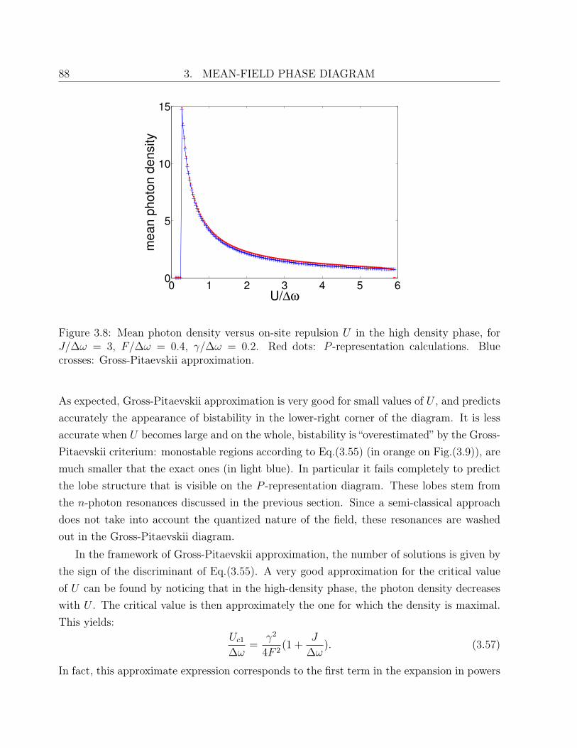
88 3. MEAN-FIELD PHASE DIAGRAM
0 1 2 3 4 5 60
5
10
15
U/∆ω
me
an
ph
oto
n d
en
sity
Figure 3.8: Mean photon density versus on-site repulsion U in the high density phase, forJ/∆ω = 3, F/∆ω = 0.4, γ/∆ω = 0.2. Red dots: P -representation calculations. Bluecrosses: Gross-Pitaevskii approximation.
As expected, Gross-Pitaevskii approximation is very good for small values of U , and predictsaccurately the appearance of bistability in the lower-right corner of the diagram. It is lessaccurate when U becomes large and on the whole, bistability is “overestimated” by the Gross-Pitaevskii criterium: monostable regions according to Eq.(3.55) (in orange on Fig.(3.9)), aremuch smaller that the exact ones (in light blue). In particular it fails completely to predictthe lobe structure that is visible on the P -representation diagram. These lobes stem fromthe n-photon resonances discussed in the previous section. Since a semi-classical approachdoes not take into account the quantized nature of the field, these resonances are washedout in the Gross-Pitaevskii diagram.
In the framework of Gross-Pitaevskii approximation, the number of solutions is given bythe sign of the discriminant of Eq.(3.55). A very good approximation for the critical valueof U can be found by noticing that in the high-density phase, the photon density decreaseswith U . The critical value is then approximately the one for which the density is maximal.This yields:
Uc1∆ω
=γ2
4F 2(1 +
J
∆ω). (3.57)
In fact, this approximate expression corresponds to the first term in the expansion in powers
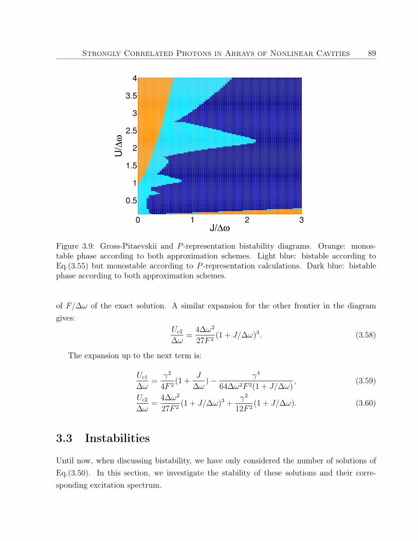
Strongly Correlated Photons in Arrays of Nonlinear Cavities 89
0 1 2 3
0.5
1
1.5
2
2.5
3
3.5
4
J/∆ω
U/∆
ω
Figure 3.9: Gross-Pitaevskii and P -representation bistability diagrams. Orange: monos-table phase according to both approximation schemes. Light blue: bistable according toEq.(3.55) but monostable according to P -representation calculations. Dark blue: bistablephase according to both approximation schemes.
of F/∆ω of the exact solution. A similar expansion for the other frontier in the diagramgives:
Uc2∆ω
=4∆ω2
27F 2(1 + J/∆ω)3. (3.58)
The expansion up to the next term is:
Uc1∆ω
=γ2
4F 2(1 +
J
∆ω)− γ4
64∆ω2F 2(1 + J/∆ω), (3.59)
Uc2∆ω
=4∆ω2
27F 2(1 + J/∆ω)3 +
γ2
12F 2(1 + J/∆ω). (3.60)
3.3 Instabilities
Until now, when discussing bistability, we have only considered the number of solutions ofEq.(3.50). In this section, we investigate the stability of these solutions and their corre-sponding excitation spectrum.
90 3. MEAN-FIELD PHASE DIAGRAM
3.3.1 Generalized Bogoliubov theory
In the theory of weakly-interacting Bose-Einstein condensates, the energy spectrum of ele-mentary excitations can be computed by taking into account small fluctuations above thecondensate and linearizing the resulting time-dependent equation. This procedure leads tothe celebrated Bogoliubov spectrum. The idea behind Bogoliubov theory can be extended todissipative systems by considering fluctuations of the density matrix around the mean-fieldsolution:
ρ =N⊗
i=1
(ρ+ δρi). (3.61)
In Bogoliubov’s original work, the key hypothesis was to assume that the operator of thecondensate mode can be approximated by a c-number. This corresponds to the Gross-Pitaevskii approximation discussed earlier. Here, we need not assume field operators to bec-numbers, the only approximation is that the density matrix remains factorized.By injecting Eq.(3.61) into the general master equation and keeping only first order termsin the fluctuations, we find linear differential equations for the coefficients of the matricesδρi. These equations are coupled in real space but decoupled in reciprocal space, due totranslational symmetry. We therefore introduce the Fourier transform of the matrices δρi:
δρk =1√N
N∑
i=1
e−ik·riδρi. (3.62)
For a 2D square lattice, the equations of evolution for δρk that stem from linearizationaround the mean-field solution are:
i∂tδρk = Lmf [δρk] + Lk[δρk], (3.63)
whereLmf [δρk] = [Hmf , δρk]− iγ
2(2bδρkb
† − b†bδρk − δρkb†b), (3.64)
andLk[δρk] = −Tk
(Tr(bδρk)[b†, ρmf ] + Tr(b†δρk)[b, ρmf ]
), (3.65)
withTk =
2J
z(cos kxa+ cos kya). (3.66)
The dispersion relation is obtained by diagonalizing the operator Lmf + Lk for every k inthe Brillouin zone. Due to dissipation, the energy spectrum is complex and the system isdynamically stable if all eigenvalues have a negative imaginary part.
Strongly Correlated Photons in Arrays of Nonlinear Cavities 91
Note that the operator Lmf is the usual Liouvillian for the effective single cavity problem.This term in Eq.(3.63) is thus independent of k. Propagation effects arise from the otherterm Lk.
Written in Fock space, Eq.(3.63) reads:
i∂tδρkn,m = [∆En −∆Em − (m+ n)
iγ
2]δρkn,m
+ (F − J〈b〉mf )(√nδρkn−1,m −
√m+ 1δρkn,m+1)
+ (F ∗ − J〈b〉∗mf )(√n+ 1δρkn+1,m −
√mδρkn,m−1)
− Tk(∑
q
√q + 1δρkq+1,q)(
√nρn−1,m −
√m+ 1ρn,m+1)
− Tk(∑
q
√q + 1δρkq,q+1)(
√n+ 1ρn+1,m −
√mρn,m−1)
+ iγ√
(n+ 1)(m+ 1)δρkn+1,m+1, (3.67)
where:
∆En = −n∆ω +Un(n− 1)
2. (3.68)
To prove that the present formalism is indeed a generalization of Bogoliubov’s theory, wefirst apply it to the equilibrium Bose-Hubbard.
3.3.2 Application to the equilibrium Bose-Hubbard model
As with the equilibrium phase diagram in the previous chapter, we begin by investigatingthe Mott insulating phase.
Excitations in the Mott phase at equilibrium
We know that at equilibrium (and zero temperature), the mean-field density matrix inthe Mott phase is a pure Fock state (the number of particles per site will be denoted by n0).Therefore, we set:
ρ = |n0〉〈n0|. (3.69)
Of course we also have in this case γ = 0 and F = 0. At this point, we need to reintroducethe chemical potential µ in order to recover equilibrium equations. From a purely formalpoint of view, all that is needed is to replace ∆ω with µ in Eq.(3.63). It should be nonetheless
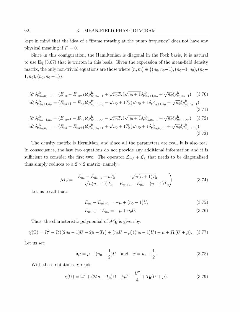
92 3. MEAN-FIELD PHASE DIAGRAM
kept in mind that the idea of a “frame rotating at the pump frequency” does not have anyphysical meaning if F = 0.
Since in this configuration, the Hamiltonian is diagonal in the Fock basis, it is naturalto use Eq.(3.67) that is written in this basis. Given the expression of the mean-field densitymatrix, the only non-trivial equations are those where (n,m) ∈ (n0, n0−1), (n0+1, n0), (n0−1, n0), (n0, n0 + 1):
i∂tδρkn0,n0−1 = (En0 − En0−1)δρkn0,n0−1 +
√n0Tk(
√n0 + 1δρkn0+1,n0
+√n0δρ
kn0,n0−1) (3.70)
i∂tδρkn0+1,n0
= (En0+1 − En0)δρkn0+1,n0
−√n0 + 1Tk(
√n0 + 1δρkn0+1,n0
+√n0δρ
kn0,n0−1)
(3.71)
i∂tδρkn0−1,n0
= (En0−1 − En0)δρkn0−1,n0
−√n0Tk(√n0 + 1δρkn0,n0+1 +
√n0δρ
kn0−1,n0
) (3.72)
i∂tδρkn0,n0+1 = (En0 − En0+1)δρkn0,n0+1 +
√n0 + 1Tk(
√n0 + 1δρkn0,n0+1 +
√n0δρ
kn0−1,n0
)
(3.73)
The density matrix is Hermitian, and since all the parameters are real, it is also real.In consequence, the last two equations do not provide any additional information and it issufficient to consider the first two. The operator Lmf + Lk that needs to be diagonalizedthus simply reduces to a 2× 2 matrix, namely:
Mk =
(En0 − En0−1 + nTk
√n(n+ 1)Tk
−√n(n+ 1))Tk En0+1 − En0 − (n+ 1)Tk
)(3.74)
Let us recall that:
En0 − En0−1 = −µ+ (n0 − 1)U, (3.75)
En0+1 − En0 = −µ+ n0U. (3.76)
Thus, the characteristic polynomial ofMk is given by:
χ(Ω) = Ω2 − Ω ((2n0 − 1)U − 2µ− Tk) + (n0U − µ)((n0 − 1)U)− µ+ Tk(U + µ). (3.77)
Let us set:
δµ = µ− (n0 −1
2)U and x = n0 +
1
2. (3.78)
With these notations, χ reads:
χ(Ω) = Ω2 + (2δµ+ Tk)Ω + δµ2 − U2
4+ Tk(U + µ). (3.79)
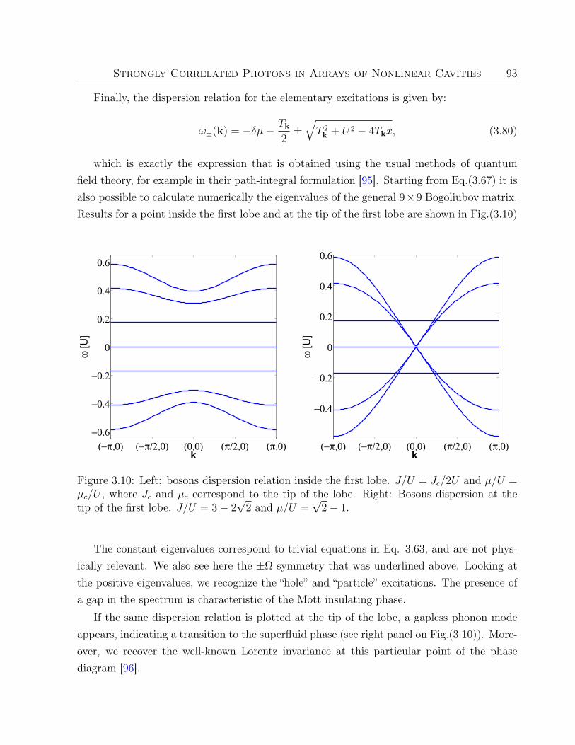
Strongly Correlated Photons in Arrays of Nonlinear Cavities 93
Finally, the dispersion relation for the elementary excitations is given by:
ω±(k) = −δµ− Tk2±√T 2k + U2 − 4Tkx, (3.80)
which is exactly the expression that is obtained using the usual methods of quantumfield theory, for example in their path-integral formulation [95]. Starting from Eq.(3.67) it isalso possible to calculate numerically the eigenvalues of the general 9×9 Bogoliubov matrix.Results for a point inside the first lobe and at the tip of the first lobe are shown in Fig.(3.10)
(−π,0) (−π/2,0) (0,0) (π/2,0) (π,0)
−0.6
−0.4
−0.2
0
0.2
0.4
0.6
k
ω [U
]
(−π,0) (−π/2,0) (0,0) (π/2,0) (π,0)
−0.4
−0.2
0
0.2
0.4
0.6
k
ω [U
]
Figure 3.10: Left: bosons dispersion relation inside the first lobe. J/U = Jc/2U and µ/U =µc/U , where Jc and µc correspond to the tip of the lobe. Right: Bosons dispersion at thetip of the first lobe. J/U = 3− 2
√2 and µ/U =
√2− 1.
The constant eigenvalues correspond to trivial equations in Eq. 3.63, and are not phys-ically relevant. We also see here the ±Ω symmetry that was underlined above. Looking atthe positive eigenvalues, we recognize the “hole” and “particle” excitations. The presence ofa gap in the spectrum is characteristic of the Mott insulating phase.
If the same dispersion relation is plotted at the tip of the lobe, a gapless phonon modeappears, indicating a transition to the superfluid phase (see right panel on Fig.(3.10)). More-over, we recover the well-known Lorentz invariance at this particular point of the phasediagram [96].
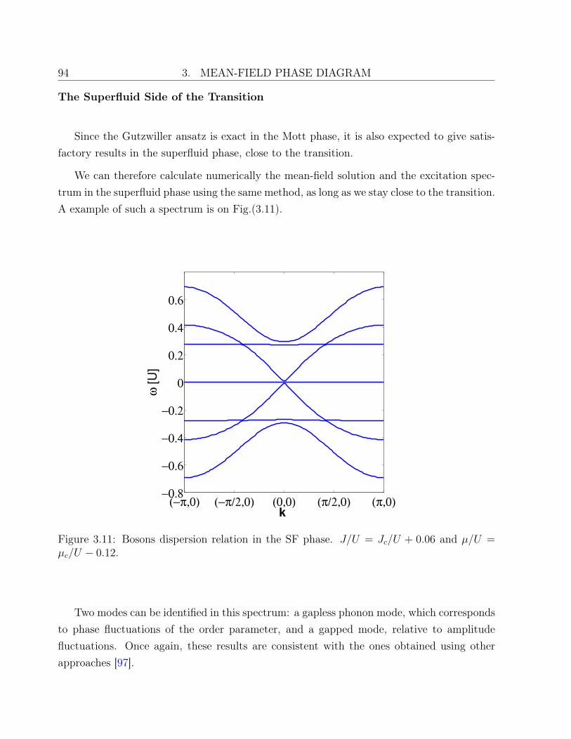
94 3. MEAN-FIELD PHASE DIAGRAM
The Superfluid Side of the Transition
Since the Gutzwiller ansatz is exact in the Mott phase, it is also expected to give satis-factory results in the superfluid phase, close to the transition.
We can therefore calculate numerically the mean-field solution and the excitation spec-trum in the superfluid phase using the same method, as long as we stay close to the transition.A example of such a spectrum is on Fig.(3.11).
(−π,0) (−π/2,0) (0,0) (π/2,0) (π,0)−0.8
−0.6
−0.4
−0.2
0
0.2
0.4
0.6
k
ω [
U]
Figure 3.11: Bosons dispersion relation in the SF phase. J/U = Jc/U + 0.06 and µ/U =µc/U − 0.12.
Two modes can be identified in this spectrum: a gapless phonon mode, which correspondsto phase fluctuations of the order parameter, and a gapped mode, relative to amplitudefluctuations. Once again, these results are consistent with the ones obtained using otherapproaches [97].
Strongly Correlated Photons in Arrays of Nonlinear Cavities 95
3.3.3 Excitation spectrum for the driven-dissipative model
Emergence of inhomogeneous phases
Equipped with the generalized Bogoliubov theory, we can now compute the excitationspectrum of the driven-dissipative model and determine the stability of the different steady-states phases. The study was carried out for the same parameters as in Fig.(3.9). Thenumber of stable solutions is shown on Fig.(3.12). As mentioned previously, in most of thebistable region, 2 out of the 3 potentially existing solutions are stable. There are howeverareas were the low-density phase becomes unstable (marked in red and yellow on Fig.(3.12)).In particular, in the region marked in red in Fig.(3.12), there is only one solution and it isunstable.
At this point, it is important to recall that within our mean-field approximation, all thesites are equivalent. Hence, we only have access to spatially homogeneous solutions. Thefact that there is no homogeneous mean-field solution for some values of the parameters, maytherefore indicate a breaking of translational symmetry and the emergence of inhomogeneousphases. Note that this kind of modulational instabilities do occur in other nonlinear opticalsystems like parametric oscillators [98].
In order to understand better this phenomenon, let us take a look at the excitationspectrum. Dispersion relations at the edge of the unstable region (points A, A’, B and B’on Fig. 3.9), are plotted on Fig. 3.13 and 3.14. We see on Fig. 3.13 and Fig. 3.14 that onthe left side of the unstable region, instabilities arise at k = (π/a, π/a). This indicates thatas we cross the unstable region from the left by increasing the coupling between cavities,an inhomogeneous density-wave steady-state occurs. Note that the other edge, the unstablek-vectors are smaller and located well inside the Brillouin zone. Another remarkable pointis that the real part of the unstable branch is zero for every k inside the Brillouin zonewhile the imaginary part is strongly dispersive. Since in the case of thermal equilibrium theexcitation spectrum is real, the existence of a purely imaginary branch is obviously relatedto dissipation. But it is interesting to note that the dispersive nature of purely imaginarybranches is a consequence of interactions. Indeed, in the low-density phase, when J U ,all eigenvalues have completely flat imaginary parts. In this regime there are two (anti-conjugate) dispersive branches whose real parts originate from the bare boson dispersion ona square lattice.
The existence of this purely imaginary branch can be seen analytically in a very lowdensity regime, assuming that there is at most one photon per site. We can then approximate
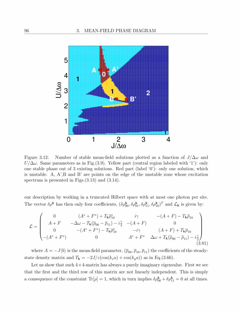
96 3. MEAN-FIELD PHASE DIAGRAM
0 1 2 3 4
1
2
3
4
5
J/∆ω
U/∆
ω
1
21
1
0
B’B
A A’
Figure 3.12: Number of stable mean-field solutions plotted as a function of J/∆ω andU/∆ω. Same parameters as in Fig.(3.9). Yellow part (central region labeled with ‘1’): onlyone stable phase out of 3 existing solutions. Red part (label ‘0’): only one solution, whichis unstable. A, A’,B and B’ are points on the edge of the unstable zone whose excitationspectrum is presented in Figs.(3.13) and (3.14).
our description by working in a truncated Hilbert space with at most one photon per site.The vector δρk has then only four coefficients, (δρk00, δρ
k01, δρ
k11, δρ
k10)T and Lk is given by:
L =
0 (A∗ + F ∗) + Tkρ∗10 iγ −(A+ F )− Tkρ10
A+ F −∆ω − Tk(ρ00 − ρ11)− iγ2−(A+ F ) 0
0 −(A∗ + F ∗)− Tkρ∗10 −iγ (A+ F ) + Tkρ10
−(A∗ + F ∗) 0 A∗ + F ∗ ∆ω + Tk(ρ00 − ρ11)− iγ2
(3.81)where A = −J〈b〉 is the mean-field parameter, (ρ00, ρ10, ρ11) the coefficients of the steady-
state density matrix and Tk = −2J/z(cos(kxa) + cos(kya)) as in Eq.(3.66).Let us show that such 4×4-matrix has always a purely imaginary eigenvalue. First we see
that the first and the third row of this matrix are not linearly independent. This is simplya consequence of the constraint Tr[ρ] = 1, which in turn implies δρk00 + δρk11 = 0 at all times.
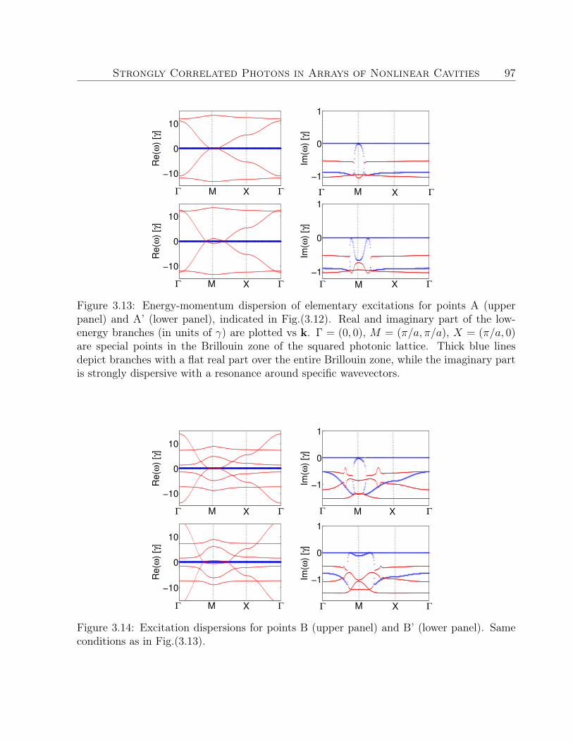
Strongly Correlated Photons in Arrays of Nonlinear Cavities 97
−10
0
10
Re
(ω)
[γ]
M ΓΓ X
−1
0
1
Im(ω
) [γ
]
ΓXMΓ
−10
0
10
Re
(ω)
[γ]
ΓXΓ M
−1
0
1
Im(ω
) [γ
]
ΓXΓ M
Figure 3.13: Energy-momentum dispersion of elementary excitations for points A (upperpanel) and A’ (lower panel), indicated in Fig.(3.12). Real and imaginary part of the low-energy branches (in units of γ) are plotted vs k. Γ = (0, 0), M = (π/a, π/a), X = (π/a, 0)are special points in the Brillouin zone of the squared photonic lattice. Thick blue linesdepict branches with a flat real part over the entire Brillouin zone, while the imaginary partis strongly dispersive with a resonance around specific wavevectors.
−10
0
10
Re
(ω)
[γ]
Γ X ΓM
−1
0
1
Im(ω
) [γ
]
ΓΓ M X
−10
0
10
Re
(ω)
[γ]
Γ X ΓM
−1
0
1
Im(ω
) [γ
]
ΓΓ M X
Figure 3.14: Excitation dispersions for points B (upper panel) and B’ (lower panel). Sameconditions as in Fig.(3.13).
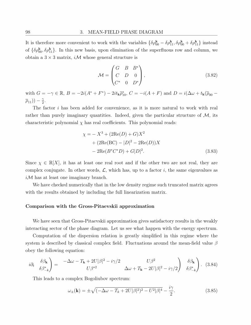
98 3. MEAN-FIELD PHASE DIAGRAM
It is therefore more convenient to work with the variables δρk00 − δρk11, δρk00 + δρk11 instead
of δρk00, δρk11. In this new basis, upon elimination of the superfluous row and column, we
obtain a 3× 3 matrix, iM whose general structure is
M =
G B B∗
C D 0
C∗ 0 D∗
, (3.82)
with G = −γ ∈ R, B = −2i(A∗ + F ∗)− 2itkρ∗10, C = −i(A + F ) and D = i(∆ω + tk(ρ00 −
ρ11))− γ2.
The factor i has been added for convenience, as it is more natural to work with realrather than purely imaginary quantities. Indeed, given the particular structure of M, itscharacteristic polynomial χ has real coefficients. This polynomial reads:
χ =−X3 + (2Re(D) +G)X2
+ (2Re(BC)− |D|2 − 2Re(D))X
− 2Re(B∗C∗D) +G|D|2. (3.83)
Since χ ∈ R[X], it has at least one real root and if the other two are not real, they arecomplex conjugate. In other words, L, which has, up to a factor i, the same eigenvalues asiM has at least one imaginary branch.
We have checked numerically that in the low density regime such truncated matrix agreeswith the results obtained by including the full linearization matrix.
Comparison with the Gross-Pitaevskii approximation
We have seen that Gross-Pitaevskii approximation gives satisfactory results in the weaklyinteracting sector of the phase diagram. Let us see what happen with the energy spectrum.
Computation of the dispersion relation is greatly simplified in this regime where thesystem is described by classical complex field. Fluctuations around the mean-field value βobey the following equation:
i∂t
(δβk
δβ∗−k
)=
(−∆ω − Tk + 2U |β|2 − iγ/2 Uβ2
Uβ∗2 ∆ω + Tk − 2U |β|2 − iγ/2
)(δβk
δβ∗−k
). (3.84)
This leads to a complex Bogoliubov spectrum:
ω±(k) = ±√
(−∆ω − Tk + 2U |β|2)2 − U2|β|4 − iγ
2. (3.85)
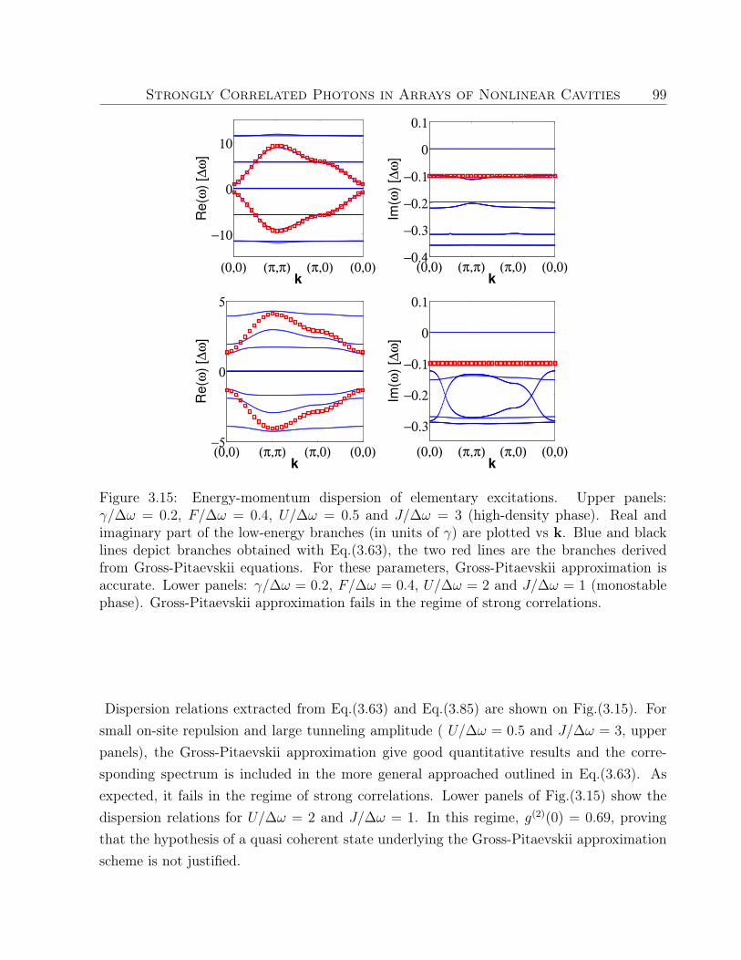
Strongly Correlated Photons in Arrays of Nonlinear Cavities 99
(0,0) (π,π) (π,0) (0,0)
−10
0
10
Re
(ω)
[∆ω
]
k(0,0) (π,π) (π,0) (0,0)
−0.4
−0.3
−0.2
−0.1
0
0.1
Im(ω
) [∆
ω]
k
(0,0) (π,π) (π,0) (0,0)−5
0
5
Re
(ω)
[∆ω
]
k(0,0) (π,π) (π,0) (0,0)
−0.3
−0.2
−0.1
0
0.1
Im(ω
) [∆
ω]
k
Figure 3.15: Energy-momentum dispersion of elementary excitations. Upper panels:γ/∆ω = 0.2, F/∆ω = 0.4, U/∆ω = 0.5 and J/∆ω = 3 (high-density phase). Real andimaginary part of the low-energy branches (in units of γ) are plotted vs k. Blue and blacklines depict branches obtained with Eq.(3.63), the two red lines are the branches derivedfrom Gross-Pitaevskii equations. For these parameters, Gross-Pitaevskii approximation isaccurate. Lower panels: γ/∆ω = 0.2, F/∆ω = 0.4, U/∆ω = 2 and J/∆ω = 1 (monostablephase). Gross-Pitaevskii approximation fails in the regime of strong correlations.
Dispersion relations extracted from Eq.(3.63) and Eq.(3.85) are shown on Fig.(3.15). Forsmall on-site repulsion and large tunneling amplitude ( U/∆ω = 0.5 and J/∆ω = 3, upperpanels), the Gross-Pitaevskii approximation give good quantitative results and the corre-sponding spectrum is included in the more general approached outlined in Eq.(3.63). Asexpected, it fails in the regime of strong correlations. Lower panels of Fig.(3.15) show thedispersion relations for U/∆ω = 2 and J/∆ω = 1. In this regime, g(2)(0) = 0.69, provingthat the hypothesis of a quasi coherent state underlying the Gross-Pitaevskii approximationscheme is not justified.
100 3. MEAN-FIELD PHASE DIAGRAM
3.4 Conclusion
In this chapter we presented an efficient method for computing the mean-field phase diagramof the driven-dissipative Bose-Hubbard model in the most general case. This method is basedon an analytical solution for the single-site problem, relying on the use of the complex P -representation.
An important feature of the mean-field phase diagram is tunneling-induced bistability.In a wide region of the diagram, the theory predicts the existence of two stable steady-states(for the same value of all the parameters). Interestingly, these two stable phases share greatsimilarities with the two types of steady-states found in Chap.2 at weak pumping and weakdissipation. Indeed, one of the phases has a high-density of photon and g(2)(0) ≤ 1. Besides,for values of U/∆ω corresponding to multiphotonic resonances and for weak tunneling rates,the light is strongly antibunched. The other phase is a low-density phase that exhibitssuperbunching near the two-photon resonance.
Remarkably, the study of stability revealed that for certain values of the parameters,collective excitations with a purely imaginary energy-momentum dispersion trigger modula-tional instabilities at specific wavevectors. This type of instabilities indicates the emergenceof inhomogeneous phases in the system.
It is noteworthy that the prediction of tunneling-induced bistability is not specific to theP -representation mean-field theory. Indeed, such phenomenon also arises within the simplerframework of the Gross-Pitaevskii equation. We have shown however that in the stronglycorrelated regime, the Gross-Pitaevskii approximation fails to give correct results.
Although it is more accurate than the Gross-Pitaevskii approach, P -representation mean-field theory is still not a fully controlled approximation. Only further studies going beyondmean-field will eventually determine its range of validity. The next chapter is a first step inthis direction.
Chapter 4
Exact numerical simulations onfinite-size systems
Although the mean-field approximation that we have used extensively so far is exact in thelimit J = 0 or U = 0, it is not a controlled approximation. It is indeed very difficult toevaluate the error on the density matrix or the observables, with respect to the exact solution.The only way to validate or invalidate the predictions of mean-field theory is therefore tocompare it with the results of other more accurate methods. To go forward in this directionwe have chosen to perform exact numerical simulations on finite-size arrays of cavities.
Simulating exactly quantum many-body systems is however a tremendous task: the di-mension of the Hilbert space for a multipartite system consisting of m subsystems, each ofthem described by a space of dimension N , is Nm. Furthermore, in nonequilibrium condi-tions, the system can no longer be described in terms of pure states, but the full densitymatrix must be considered. In this case, the number of variables to be determined scales asN2m, namely the square of the size of the Hilbert space. In the case of cavity arrays wherewe may have to consider 3 or 4 photons per site, the problem becomes quickly intractablewith brute-force methods, even for relatively small lattices: the dimension of the Hilbertspace for a 3× 3 square lattice with up to 4 photons per cavity is already 59 ' 2× 10⁶.
In this context, the need for a new and efficient method for simulating two-dimensionaldriven-dissipative systems gave rise to an ambitious project that was started with AlexandreBaksic and Stefano Finazzi, under the supervision of Cristiano Ciuti. We were later joinedby Florent Storme and are still actively working on the subject. As a result, rather thanpresenting a systematic study of the validity of the mean-field approximation, this chapterwill focus on the main ideas and the first results of this new numerical method.
The main purpose of the method is to simplify the initial problem by restricting the time
101
102 4. EXACT NUMERICAL SIMULATIONS ON FINITE-SIZE SYSTEMS
evolution of the system to a small “corner” of the Hilbert space that would contain all therelevant many-body states. The accuracy of the results can then be improved by increasingthe size of the corner until convergence (in the value of the observables) is reached.
We have developed two types of “corner method”. In the first approach, we select themost probable states at the single-site level by diagonalizing the mean-field density matrix.The corner basis is then formed by taking the most probable products of single-site states.We will see that this approach has better performance than a direct simulation in Fock statebut still has limitations in lattice size. The second, more sophisticated approach is based ona real-space renormalization procedure. The corner basis is constructed by merging smallerlattices and selecting the most probable product states. An article presenting the results ofthis second approach is currently under review [24].
Strongly Correlated Photons in Arrays of Nonlinear Cavities 103
4.1 A first approach: Selecting a corner space from the
mean-field density matrix
The very general idea of selecting a small portion of a gigantic Hilbert space has been atthe heart of several approximation schemes developed in the last decades. Most of theseworks were devoted to equilibrium systems for which the fundamental task is to find themany-body ground state. The first attempt in this direction was the renormalization grouptechnique, proposed by Wilson and successfully applied to the Kondo problem [99]. Numer-ical implementations of this approach are based on the solution of a system with a smallerHilbert space, where only the relevant physical states with the lower energy are retained.Ideally this procedure can be iterated by arbitrarily growing the size of the system step bystep, by doubling it, for instance, at each iteration. Unfortunately, such a naive numericalimplementation of the real-space renormalization group often yields poor results for nondis-sipative quantum lattice systems, because the boundary conditions imposed while solvingthe smaller system are generally not appropriate to describe the doubled one [100].
In the case of one-dimensional systems, a solution to this impasse is represented by thedensity matrix renormalization group (DMRG) [101], a more sophisticated technique whichprovides extremely precise results, often up to numerical precision, and which is based on theselection of most probable states of a properly constructed reduced density matrix. Behindthe success of this method lies the fact that it operates on a very specific class of quantumstates called matrix-product states (MPS) [102]. Generalization of this technique for spatialdimension larger than one have been introduced, based on an artificial description in termsof one-dimensional systems with long-range interactions [103] or through the generalizationof matrix product states to projected entangled-pair states (PEPS) [104]. However, goingfrom one to two spatial dimension makes all the calculations much more difficult. Hence,improving the efficiency of these algorithms is still a subject of intense research.
These approaches, and in particular the DMRG procedure for 1D-systems, can be gener-alized to open systems by working in the super-Hilbert space of density matrices [105, 106,107, 108]. The price to pay is to add another level of complexity, which is still manageablefor 1D systems but makes 2D problems even more difficult to tackle.
We have explored an alternative route and developed a new method that is well suitedfor dealing with two-dimensional systems such as arrays of nonlinear cavities. As alreadymentioned, the objective is to find a way to classify the states and select the most relevant
104 4. EXACT NUMERICAL SIMULATIONS ON FINITE-SIZE SYSTEMS
ones. One way of doing so is to find an approximate density matrix in the total Hilbert space,which can be readily diagonalized. In the basis in which this density matrix in diagonal,a certain probability is associated to each of the state-vectors. The subspace generated bythe most probable states is then a good candidate for the “corner space”. In this section,we describe a first implementation of this idea, taking the mean-field density matrix as anapproximate solution. The different steps of the procedure, presented in details below, arethe following:
1. Diagonalize the single-site mean-field density matrix.
2. Select the M most probable product states as a basis for the corner space.
3. Determine the steady-state solution of the density matrix in the corner space.
4. Increase M until convergence is reached for all the observables.
4.1.1 Main steps of the algorithm
Step 1: Diagonalization of the mean-field density matrix
The first step for the selection of the most probable states is to diagonalize the single-sitemean-field density matrix:
ρ(MF ) =∑
j
p(MF )j |ψ(MF )
j 〉〈ψ(MF )j |, (4.1)
where the states are ordered in such a way that:
p(MF )j ≥ p
(MF )j+1 . (4.2)
Note that before diagonalization, the density matrix is typically represented in the Fock basis.For all practical purposes, one always has to set a maximum number of photons per siteNmax,which will in turn determine the maximum number of eigenstates |ψ(MF )
0 〉, |ψ(MF )1 〉 . . . |ψ(MF )
Nmax〉,
of the mean-field density matrix that will be taken into account. This cutoff Nmax has tobe large enough to ensure convergence of the mean-field solution. If however the probabilitydistribution of the eigenstates is concentrated on a few states, the number of states per sitethat will eventually contribute to the steady-state may be much smaller than Nmax.
Strongly Correlated Photons in Arrays of Nonlinear Cavities 105
Step 2: Selection of the most probable product states as a basis for the cornerspace
Once the diagonal form of the mean-field density matrix in known, the states spanningthe corner space are chosen in the following way: to select a corner space of size M , we keepthe M most probable product states of the form
|ψ(MF )rj(1) 〉|ψ
(MF )rj(2) 〉 . . . |ψ
(MF )rj(Nsite)
〉, (4.3)
ranked according to the joint probability p(MF )rj(1) p
(MF )rj(2) . . . p
(MF )rj(Nsite)
, where the indices indicatingthe rank are such that:
p(MF )rj(1) p
(MF )rj(2) . . . p
(MF )rj(Nsite)
≥ p(MF )rj+1(1)p
(MF )rj+1(2) . . . p
(MF )rj+1(Nsite)
. (4.4)
These states form an orthonormal basis of the corner space.Note that in the expression above, one can have p(MF )
rj(k) < p(MF )rj+1(k) for some site indices
even though the product of the probabilities is such that Eq.(4.4) is satisfied. It occurs, forexample, if the probability distribution in Eq.(4.1) is such that
p(MF )1 p
(MF )1 > p
(MF )0 p
(MF )2 . (4.5)
It is then more probable to have two sites in |ψ(MF )1 〉 than one site in |ψ(MF )
2 〉 and one in|ψ(MF )
0 〉.The Hilbert space generated by the product states of Eq.(4.3) can be viewed as composed
of several “shells” containing states with the same probability. Indeed, the probability of astate is entirely determined by a vector (n0, n1, . . . , nNmax), with
Nmax∑
j=0
nj = Nsite, (4.6)
denoting the number of sites in states |ψ(MF )0 〉, |ψ(MF )
1 〉 . . . |ψ(MF )Nmax〉 respectively. This vector
defines a shell of states that are all related by an arbitrary permutation of the lattice sitesleaving (n0, n1, . . . , nNmax) unchanged. As a result, the number of states of a single shell isgiven by the multinomial coefficients
S(n0, n1, . . . , nNmax) =Nsite!∏Nmaxj=0 nj!
, (4.7)
106 4. EXACT NUMERICAL SIMULATIONS ON FINITE-SIZE SYSTEMS
and their probability is
p(n0, n1, . . . , nNmax) =Nmax∏
j=0
(p
(MF )j
)nj. (4.8)
For example, the most probable shell is (Nsite, 0, . . . , 0), which corresponds to the uniquestate where all sites are in |ψ(MF )
0 〉. The second most probable is (Nsite − 1, 1, 0, . . . , 0), forwhich one of the sites is in |ψ(MF )
1 〉 and all the others in |ψ(MF )0 〉. We see that the selection
of the state spanning the corner amounts to selecting the most probable shells, so that thenumber of total states in the corner is equal to M .
Once the M basis vectors of the corner space have been identified, the next task is toproject all the operators governing the dynamics of the system on the corner space. One ofthe simplest ways to do so would be to write the matrix representation of the operators inthe full space and delete afterwards the rows and columns corresponding to vectors layingoutside of the corner space. However, for large lattices, this method requires the creationand manipulation of very large matrices. To avoid this difficulty, we have used an alternativeway of projecting the operators on the corner space that is more efficient in terms of memoryand do not require to write matrices in the full Hilbert space. Details on this procedure arepresented in Appendix B.
At the end of step 2, we have at our disposal the matrix representation of all the relevantoperators projected in the corner space.
Step 3: Determination of the steady-state density matrix in the corner space
The steady state of the system is determined by solving the master equation in the cornerspace. We assume that the master equation has the same form as Eq.(1.106), namely:
i∂tρ = [H, ρ] +iγ
2
Nsite∑
i=1
[2biρb
†i − b†ibiρ− ρb†ibi
], (4.9)
where all the operators are restricted to the corner space. There are several ways to findnumerically the steady-states of Eq.(4.9). Usually, for a small corner space C(M), the fastestway is to solve Eq.(4.9) directly, in the vector space of operators on C(M), of which thedensity matrices form a convex set. This can be done by diagonalizing the Liouvilliansuperoperator
L = [H, •]− iγ
2
Nsites∑
i=1
[2bi • b†i − b†ibi •+ • b†ibi
], (4.10)
Strongly Correlated Photons in Arrays of Nonlinear Cavities 107
acting on ρ seen as a vector. Eigenvectors corresponding to the eigenvalue 0 are steady-statesof the system. Alternatively, one can solve the differential equation Eq.(4.9) by using, e.g.,Runge-Kutta algorithms, until the system reaches a stationary state.
These methods are fully deterministic and their precision is limited only by the perfor-mance of the diagonalization or time evolution algorithms. However, as they require to workin the space of operators, which has a dimension M2, they are very demanding in termsof memory. In practice they are manageable as long as M < 103. When the dimensionof the corner space is increased further, a Monte Carlo wave-function technique is needed[109, 110, 111, 112]. In this stochastic approach, which is detailed in Appendix A, the mas-ter equation is solved by averaging over quantum trajectories of pure states in presence ofrandom quantum jumps. As the time evolution is performed on pure states, the matricesinvolved in the algorithm have a dimension M instead of M2. With this technique, a sizeM ∼ 104 is reachable, depending on the sparsity of the matrices.
Step 4: Increasing M until convergence is reached
The accuracy of the results is checked by increasing the size M of the corner space untilconvergence in the value of the observables is reached. We emphasize that in principle, byincreasing arbitrarily M , the method becomes exact since the considered basis spans theentire Hilbert space. Of course, in practice, the method is useful when the number of statesrequired to reach convergence is small enough to be treated numerically.
Note that although the basis spanning the corner space is formed by factorized states, withno correlations between different sites, the final steady-state may contain such correlationsas it involves linear superpositions of the basis vectors.
4.1.2 Results
Although the method presented above is not restricted to any particular lattice model, wehave first implemented it for the driven-dissipative Bose-Hubbard model on a 2 × 2 squarelattice with periodic boundary conditions. For such a small number of sites, the size of theHilbert space is reasonable. Setting a cutoff of Nmax = 4 photons per site, the dimension ofthe total space is only 54 = 625, which makes it possible to solve directly the master equationwithout resorting to wave-function Monte Carlo calculations. Figures 4.1 and 4.2 show themean photon density and g(2)(0) in the steady-states, as a function of the number of states
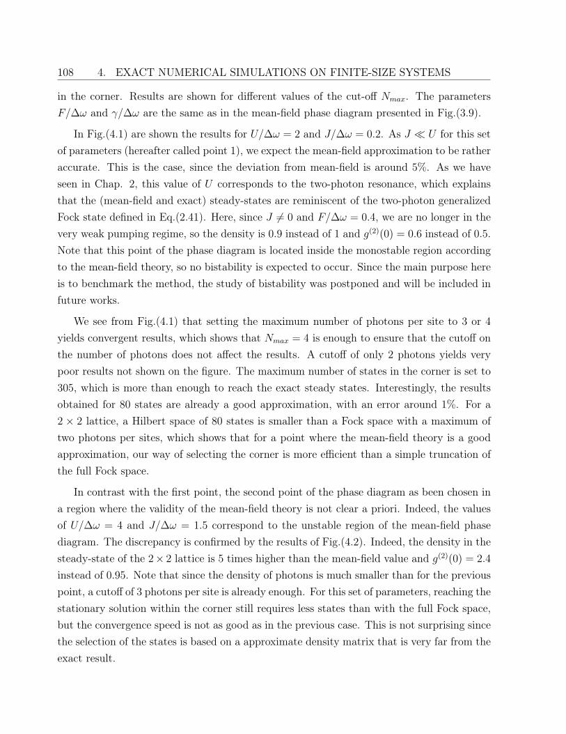
108 4. EXACT NUMERICAL SIMULATIONS ON FINITE-SIZE SYSTEMS
in the corner. Results are shown for different values of the cut-off Nmax. The parametersF/∆ω and γ/∆ω are the same as in the mean-field phase diagram presented in Fig.(3.9).
In Fig.(4.1) are shown the results for U/∆ω = 2 and J/∆ω = 0.2. As J U for this setof parameters (hereafter called point 1), we expect the mean-field approximation to be ratheraccurate. This is the case, since the deviation from mean-field is around 5%. As we haveseen in Chap. 2, this value of U corresponds to the two-photon resonance, which explainsthat the (mean-field and exact) steady-states are reminiscent of the two-photon generalizedFock state defined in Eq.(2.41). Here, since J 6= 0 and F/∆ω = 0.4, we are no longer in thevery weak pumping regime, so the density is 0.9 instead of 1 and g(2)(0) = 0.6 instead of 0.5.Note that this point of the phase diagram is located inside the monostable region accordingto the mean-field theory, so no bistability is expected to occur. Since the main purpose hereis to benchmark the method, the study of bistability was postponed and will be included infuture works.
We see from Fig.(4.1) that setting the maximum number of photons per site to 3 or 4
yields convergent results, which shows that Nmax = 4 is enough to ensure that the cutoff onthe number of photons does not affect the results. A cutoff of only 2 photons yields verypoor results not shown on the figure. The maximum number of states in the corner is set to305, which is more than enough to reach the exact steady states. Interestingly, the resultsobtained for 80 states are already a good approximation, with an error around 1%. For a2 × 2 lattice, a Hilbert space of 80 states is smaller than a Fock space with a maximum oftwo photons per sites, which shows that for a point where the mean-field theory is a goodapproximation, our way of selecting the corner is more efficient than a simple truncation ofthe full Fock space.
In contrast with the first point, the second point of the phase diagram as been chosen ina region where the validity of the mean-field theory is not clear a priori. Indeed, the valuesof U/∆ω = 4 and J/∆ω = 1.5 correspond to the unstable region of the mean-field phasediagram. The discrepancy is confirmed by the results of Fig.(4.2). Indeed, the density in thesteady-state of the 2× 2 lattice is 5 times higher than the mean-field value and g(2)(0) = 2.4
instead of 0.95. Note that since the density of photons is much smaller than for the previouspoint, a cutoff of 3 photons per site is already enough. For this set of parameters, reaching thestationary solution within the corner still requires less states than with the full Fock space,but the convergence speed is not as good as in the previous case. This is not surprising sincethe selection of the states is based on a approximate density matrix that is very far from theexact result.

Strongly Correlated Photons in Arrays of Nonlinear Cavities 109
0 100 200 3000.8
0.85
0.9
0.95
1
M
Me
an
ph
oto
n d
en
sity
Nmax
= 4
Nmax
= 3
MF value
0 100 200 3000.45
0.5
0.55
0.6
0.65
M
g2(0
)
Nmax
= 3
Nmax
= 4
MF value
Figure 4.1: Mean photon density and g2(0) as a function of the number of states in thecorner space for a 2× 2 lattice. Point 1: U/∆ω = 2, J/∆ω = 0.2, F/∆ω = 0.4, γ/∆ω = 0.2.Dashed black line: mean-field solution
0 100 200 3000.02
0.04
0.06
0.08
0.1
0.12
0.14
0.16
M
Me
an
ph
oto
n d
en
sity
Nmax
= 3
Nmax
= 4
MF valueN
max = 2
0 100 200 300 4000
0.5
1
1.5
2
2.5
M
g2(0
)
Nmax
=4
Nmax
= 3
MF valueN
max = 2
Figure 4.2: Mean photon density and g2(0) as a function of the number of states in thecorner space for a 2× 2 lattice. Point 2: U/∆ω = 4, J/∆ω = 1.5, F/∆ω = 0.4, γ/∆ω = 0.2.Dashed black line: mean-field solution.
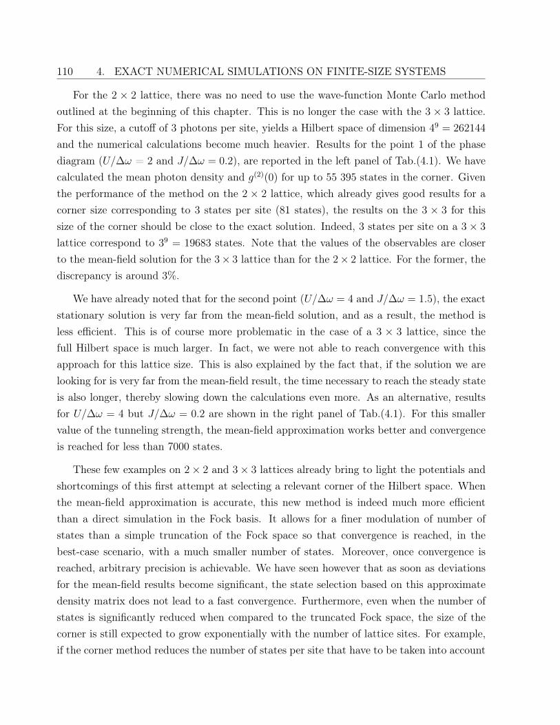
110 4. EXACT NUMERICAL SIMULATIONS ON FINITE-SIZE SYSTEMS
For the 2 × 2 lattice, there was no need to use the wave-function Monte Carlo methodoutlined at the beginning of this chapter. This is no longer the case with the 3 × 3 lattice.For this size, a cutoff of 3 photons per site, yields a Hilbert space of dimension 49 = 262144
and the numerical calculations become much heavier. Results for the point 1 of the phasediagram (U/∆ω = 2 and J/∆ω = 0.2), are reported in the left panel of Tab.(4.1). We havecalculated the mean photon density and g(2)(0) for up to 55 395 states in the corner. Giventhe performance of the method on the 2 × 2 lattice, which already gives good results for acorner size corresponding to 3 states per site (81 states), the results on the 3 × 3 for thissize of the corner should be close to the exact solution. Indeed, 3 states per site on a 3× 3
lattice correspond to 39 = 19683 states. Note that the values of the observables are closerto the mean-field solution for the 3× 3 lattice than for the 2× 2 lattice. For the former, thediscrepancy is around 3%.
We have already noted that for the second point (U/∆ω = 4 and J/∆ω = 1.5), the exactstationary solution is very far from the mean-field solution, and as a result, the method isless efficient. This is of course more problematic in the case of a 3 × 3 lattice, since thefull Hilbert space is much larger. In fact, we were not able to reach convergence with thisapproach for this lattice size. This is also explained by the fact that, if the solution we arelooking for is very far from the mean-field result, the time necessary to reach the steady stateis also longer, thereby slowing down the calculations even more. As an alternative, resultsfor U/∆ω = 4 but J/∆ω = 0.2 are shown in the right panel of Tab.(4.1). For this smallervalue of the tunneling strength, the mean-field approximation works better and convergenceis reached for less than 7000 states.
These few examples on 2× 2 and 3× 3 lattices already bring to light the potentials andshortcomings of this first attempt at selecting a relevant corner of the Hilbert space. Whenthe mean-field approximation is accurate, this new method is indeed much more efficientthan a direct simulation in the Fock basis. It allows for a finer modulation of number ofstates than a simple truncation of the Fock space so that convergence is reached, in thebest-case scenario, with a much smaller number of states. Moreover, once convergence isreached, arbitrary precision is achievable. We have seen however that as soon as deviationsfor the mean-field results become significant, the state selection based on this approximatedensity matrix does not lead to a fast convergence. Furthermore, even when the number ofstates is significantly reduced when compared to the truncated Fock space, the size of thecorner is still expected to grow exponentially with the number of lattice sites. For example,if the corner method reduces the number of states per site that have to be taken into account
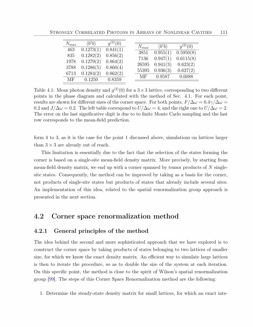
Strongly Correlated Photons in Arrays of Nonlinear Cavities 111
Nmax 〈b†b〉 g(2)(0)463 0.1273(1) 0.841(1)835 0.1282(2) 0.856(2)1978 0.1279(2) 0.864(2)3788 0.1286(5) 0.860(4)6713 0.1284(2) 0.862(2)MF 0.1250 0.8359
Nmax 〈b†b〉 g(2)(0)3851 0.955(1) 0.5950(8)7136 0.947(1) 0.6115(8)26595 0.941(3) 0.623(2)55395 0.936(3) 0.627(2)MF 0.9587 0.6088
Table 4.1: Mean photon density and g(2)(0) for a 3×3 lattice, corresponding to two differentpoints in the phase diagram and calculated with the method of Sec. 4.1. For each point,results are shown for different sizes of the corner space. For both points, F/∆ω = 0.4γ/∆ω =0.2 and J/∆ω = 0.2. The left table correspond to U/∆ω = 4, and the right one to U/∆ω = 2.The error on the last significative digit is due to to finite Monte Carlo sampling and the lastrow corresponds to the mean-field prediction.
form 4 to 3, as it is the case for the point 1 discussed above, simulations on lattices largerthan 3× 3 are already out of reach.
This limitation is essentially due to the fact that the selection of the states forming thecorner is based on a single-site mean-field density matrix. More precisely, by starting frommean-field density matrix, we end up with a corner spanned by tensor products of N single-site states. Consequently, the method can be improved by taking as a basis for the corner,not products of single-site states but products of states that already include several sites.An implementation of this idea, related to the spatial renormalization group approach ispresented in the next section.
4.2 Corner space renormalization method
4.2.1 General principles of the method
The idea behind the second and more sophisticated approach that we have explored is toconstruct the corner space by taking products of states belonging to two lattices of smallersize, for which we know the exact density matrix. An efficient way to simulate large latticesis then to iterate the procedure, so as to double the size of the system at each iteration.On this specific point, the method is close to the spirit of Wilson’s spatial renormalizationgroup [99]. The steps of this Corner Space Renormalization method are the following:
1. Determine the steady-state density matrix for small lattices, for which an exact inte-
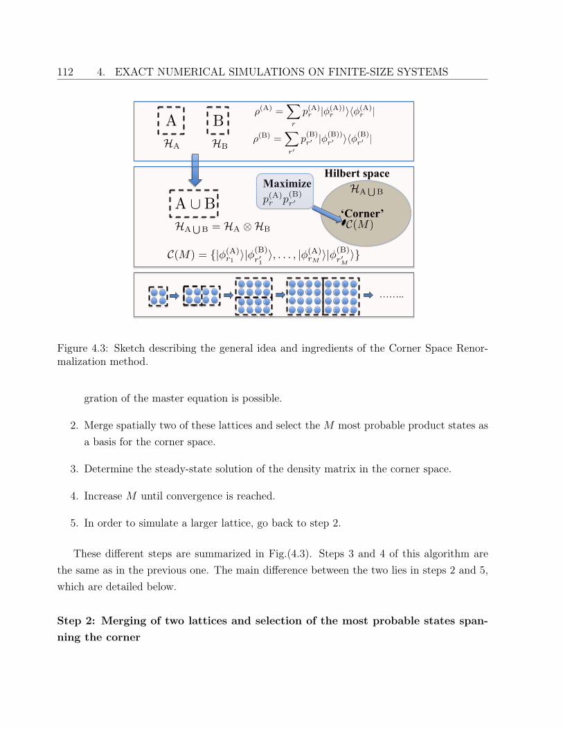
112 4. EXACT NUMERICAL SIMULATIONS ON FINITE-SIZE SYSTEMS
‘Corner’
Maximize
Hilbert space
A B
A [ B
HA HB
(A) =X
r
p(A)r |(A))
r ih(A)r |
HAS
B = HA HB
C(M) = |(A)r1
i|(B)r01i, . . . , |(A)
rMi|(B)
r0Mi
C(M)
HAS
Bp(A)
r p(B)r0
(B) =X
r0
p(B)r0 |(B))
r0 ih(B)r0 |
……..
Figure 4.3: Sketch describing the general idea and ingredients of the Corner Space Renor-malization method.
gration of the master equation is possible.
2. Merge spatially two of these lattices and select the M most probable product states asa basis for the corner space.
3. Determine the steady-state solution of the density matrix in the corner space.
4. Increase M until convergence is reached.
5. In order to simulate a larger lattice, go back to step 2.
These different steps are summarized in Fig.(4.3). Steps 3 and 4 of this algorithm arethe same as in the previous one. The main difference between the two lies in steps 2 and 5,which are detailed below.
Step 2: Merging of two lattices and selection of the most probable states span-ning the corner
Strongly Correlated Photons in Arrays of Nonlinear Cavities 113
Let us suppose that we know the steady-state density matrices ρ(A) and ρ(B) for twolattices A and B. The goal is to use these solutions to select the relevant corner for the largerlattice obtained by merging spatially A and B. Note that the corresponding Hilbert space isthen H(A∪B) = HA ⊗HB where HA and HB are the Hilbert spaces of systems A and B.
The procedure for selecting the most relevant states is then quite similar to what hasbeen presented previously. Each density-matrix operator can be diagonalized as:
ρ(A) =∑
r
p(A)r |φ(A))
r 〉〈φ(A)r |, (4.11)
where the states |φ(A)r 〉 form an orthonormal basis for the Hilbert space HA of A and pA
r arethe corresponding probabilities (analogous notations hold for the quantities relating to theother subsystem B). The corner is then spanned by the most probable states of the form
|φ(A)rj〉 ⊗ |φ(B)
r′j〉, (4.12)
according to their joint probability p(A)rj p
(B)
r′j. As in the previous section the rank indices are
such that:
p(A)r1p
(B)
r′1≥ p(A)
r2p
(B)
r′2≥ ... ≥ p(A)
rMp
(B)
r′M, (4.13)
and the corner space is spanned by the orthonormal basis states
|φ(A)r1〉|φ(B)
r′1〉, |φ(A)
r2〉|φ(B)
r′2〉, ..., |φ(A)
rM〉|φ(B)
r′M〉. (4.14)
The lattices A and B are not necessarily identical and the code we have developed isdesigned to be as general as possible. The properties of a lattice and its associated Hamil-tonian is encoded in a specific class of objects. In particular, the geometry of the lattice isstored as an attribute of this class. The merging of two lattices is then done by defining anew instance of the class with a new geometry, and by building all the operators associatedwith this new geometry. To be compatible with different types of lattices, the geometry isdefined by the links between the sites. In view of the merging procedure, it was also usefulto distinguish between internal and external links: external links represent the boundaryconditions and are the one that may be broken and redefined when connecting two latticestogether, while internal links do not change in the merging process.
Once the geometry of the new lattice A ∪ B is defined, the next task is to compute theoperators in the new corner. The tunneling operators that correspond to internal links inthe lattice as well as all the operators acting only on a single site of the lattice, can be
114 4. EXACT NUMERICAL SIMULATIONS ON FINITE-SIZE SYSTEMS
constructed in the same way. Let us take the example of an annihilation operator. If a sitej belongs to lattice B, then
bj = I(A) ⊗ b(B)j , (4.15)
where I(A) is the Identity matrix acting in the Hilbert space HA. The expression for thetunneling operators connecting the two lattice is of the form:
b†ibj = b(A)†i ⊗ b(B)
j , (4.16)
where the two sites i and j, belong to lattice A and B respectively. The new Hamiltonian isthen defined by:
H(C) = H(A) ⊗ I(B) + I(A) ⊗H(B) + JA−B, (4.17)
where H(A) and H(B) are the Hamiltonians of the lattices A and B, and JA−B is an operatorincluding all tunneling operators coupling the two lattices. The latter is therefore definedby:
JA−B = −J∑
<i∈α,j∈β>
(b
(A)†i ⊗ b(B)
j + b(A)i ⊗ b(B)†
j
), (4.18)
where α and β denote the sites on the common edge of the two lattices. Of course, the sizeof the corner is most of the time much smaller than the Hilbert space H(A∪B). This meansthat in the matrix representation of the operators defined above, only rows and columncorresponding to states belonging to the selected corner are to be kept.
Step 5: Iteration of the procedure
For homogeneous systems, an efficient way to iterate the procedure is to choose A and Bas identical, so as to double the size of the system at each iteration. This iterative processmakes this method much more powerful than the one described in the previous section.Indeed, with this approach the knowledge gained in simulating a N -site lattice is exploitedto solve the 2N -site problem, whereas it is “waisted” if one starts from the mean-field densitymatrix for each lattice size.
Besides, in the Corner Space Renormalization method, correlations between sites aretreated exactly within the subsystems A and B. As a result, a selection of the states basedon the approximate density matrix ρ(A) ⊗ ρ(B) is more efficient than the one based on thesingle-site mean-field solution
⊗Ni=1 ρMF.
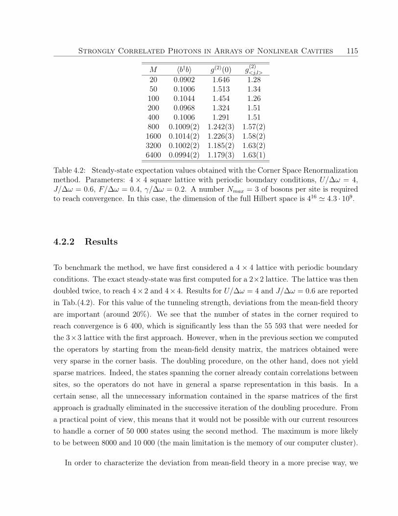
Strongly Correlated Photons in Arrays of Nonlinear Cavities 115
M 〈b†b〉 g(2)(0) g(2)<j,l>
20 0.0902 1.646 1.2850 0.1006 1.513 1.34100 0.1044 1.454 1.26200 0.0968 1.324 1.51400 0.1006 1.291 1.51800 0.1009(2) 1.242(3) 1.57(2)1600 0.1014(2) 1.226(3) 1.58(2)3200 0.1002(2) 1.185(2) 1.63(2)6400 0.0994(2) 1.179(3) 1.63(1)
Table 4.2: Steady-state expectation values obtained with the Corner Space Renormalizationmethod. Parameters: 4 × 4 square lattice with periodic boundary conditions, U/∆ω = 4,J/∆ω = 0.6, F/∆ω = 0.4, γ/∆ω = 0.2. A number Nmax = 3 of bosons per site is requiredto reach convergence. In this case, the dimension of the full Hilbert space is 416 ' 4.3 · 109.
4.2.2 Results
To benchmark the method, we have first considered a 4 × 4 lattice with periodic boundaryconditions. The exact steady-state was first computed for a 2×2 lattice. The lattice was thendoubled twice, to reach 4×2 and 4×4. Results for U/∆ω = 4 and J/∆ω = 0.6 are reportedin Tab.(4.2). For this value of the tunneling strength, deviations from the mean-field theoryare important (around 20%). We see that the number of states in the corner required toreach convergence is 6 400, which is significantly less than the 55 593 that were needed forthe 3×3 lattice with the first approach. However, when in the previous section we computedthe operators by starting from the mean-field density matrix, the matrices obtained werevery sparse in the corner basis. The doubling procedure, on the other hand, does not yieldsparse matrices. Indeed, the states spanning the corner already contain correlations betweensites, so the operators do not have in general a sparse representation in this basis. In acertain sense, all the unnecessary information contained in the sparse matrices of the firstapproach is gradually eliminated in the successive iteration of the doubling procedure. Froma practical point of view, this means that it would not be possible with our current resourcesto handle a corner of 50 000 states using the second method. The maximum is more likelyto be between 8000 and 10 000 (the main limitation is the memory of our computer cluster).
In order to characterize the deviation from mean-field theory in a more precise way, we
116 4. EXACT NUMERICAL SIMULATIONS ON FINITE-SIZE SYSTEMS
have computed the nearest-neighbor correlation function:
g(2)<j,l> =
〈b†jb†l bjbl〉〈b†jbj〉〈b†l bl〉
. (4.19)
Note that we recover the on-site correlation function g(2)(0) for i = l. By definition thisfunction is constant and equal to 1 for the mean-field solution. As seen is Tab.(4.2), g(2)
<j,l> '1.6 in the stationary solution, which confirms that this method is able to restore correlationsbetween neighboring sites that are neglected at the mean-field level.
We have also tried to combine this second method with the first one. We have calculatedthe steady-states for a 3× 3 lattice using the first method (which is still much more efficientthan using a truncated Fock basis), and used this result to simulate a 3 × 6 lattice. Anexample of time evolution for different lattice sizes is shown in Fig.(4.4). The parameters ofthe Hamiltonian are the same as in Tab.(4.2). We see that, although the deviation from themean-field solution remains significant, it decreases as the system size is increased. What iseven more interesting is that close results are obtained for 3 × 3, 4 × 4 and 6 × 3 lattices,indicating that we are approaching the result for the thermodynamical limit.
A summary of all the results obtained so far is presented in Tab.(4.3). Remarkably, thecorner size (necessary to reach convergence) does not grow exponentially with the size of thelattice but seems to follow a power law. It is however too early to establish any precise scalingbehavior. In particular, the performance of the method depends strongly on the parametersof the Hamiltonian. For hard-core (U =∞), or weakly interacting bosons (U → 0), accurateresults can be reached very quickly. The convergence is much slower in strongly correlatedphases, when U and J are of the same order of magnitude and both large when comparedwith the other parameters of the system.
Another conclusion to be drawn from Tab.(4.3) is that mean-field theory works quite wellfor small values of J/∆ω, of the order of 0.2.
4.3 Conclusion and outlook
In order to go beyond the mean-field approximation in our investigation of the driven-dissipative Bose-Hubbard model, we have developed a new numerical method for simulatingdriven-dissipative arrays of cavities that is well suited for handling lattices with more thanone spatial dimension. The general idea behind this method is to select a small corner ofthe Hilbert space, where the master equation for the density matrix is solved by using, e.g„a wave-function Monte Carlo algorithm.
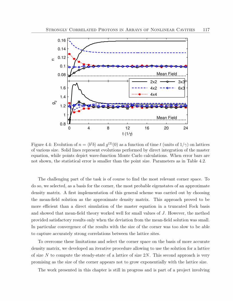
Strongly Correlated Photons in Arrays of Nonlinear Cavities 117
0.08
0.1
0.12
0.14
0.16
Time
n
Mean Field
0 4 8 12 16 20 240.8
1
1.2
1.4
1.6
t (1/γ)
g2
Mean Field
2x2
4x2
4x4
3x3
6x3
Figure 4.4: Evolution of n = 〈b†b〉 and g(2)(0) as a function of time t (units of 1/γ) on latticesof various size. Solid lines represent evolutions performed by direct integration of the masterequation, while points depict wave-function Monte Carlo calculations. When error bars arenot shown, the statistical error is smaller than the point size. Parameters as in Table 4.2.
The challenging part of the task is of course to find the most relevant corner space. Todo so, we selected, as a basis for the corner, the most probable eigenstates of an approximatedensity matrix. A first implementation of this general scheme was carried out by choosingthe mean-field solution as the approximate density matrix. This approach proved to bemore efficient than a direct simulation of the master equation in a truncated Fock basisand showed that mean-field theory worked well for small values of J . However, the methodprovided satisfactory results only when the deviation from the mean-field solution was small.In particular convergence of the results with the size of the corner was too slow to be ableto capture accurately strong correlations between the lattice sites.
To overcome these limitations and select the corner space on the basis of more accuratedensity matrix, we developed an iterative procedure allowing to use the solution for a latticeof size N to compute the steady-state of a lattice of size 2N . This second approach is verypromising as the size of the corner appears not to grow exponentially with the lattice size.
The work presented in this chapter is still in progress and is part of a project involving
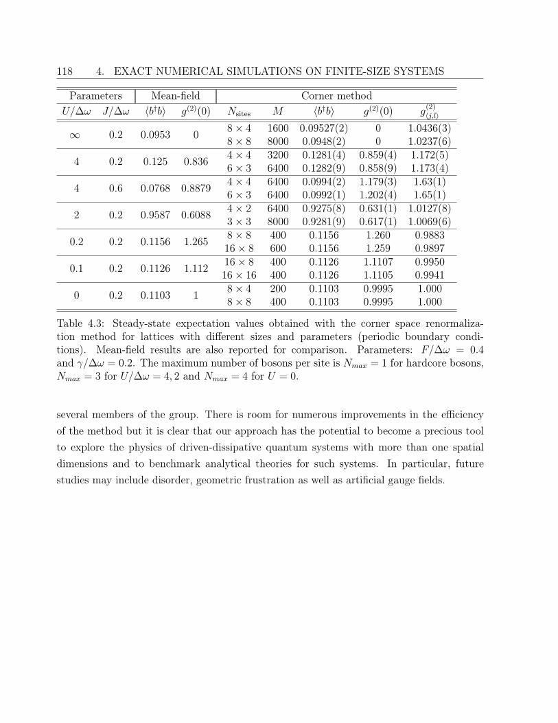
118 4. EXACT NUMERICAL SIMULATIONS ON FINITE-SIZE SYSTEMS
Parameters Mean-field Corner methodU/∆ω J/∆ω 〈b†b〉 g(2)(0) Nsites M 〈b†b〉 g(2)(0) g
(2)〈j,l〉
∞ 0.2 0.0953 0 8× 4 1600 0.09527(2) 0 1.0436(3)8× 8 8000 0.0948(2) 0 1.0237(6)
4 0.2 0.125 0.836 4× 4 3200 0.1281(4) 0.859(4) 1.172(5)6× 3 6400 0.1282(9) 0.858(9) 1.173(4)
4 0.6 0.0768 0.8879 4× 4 6400 0.0994(2) 1.179(3) 1.63(1)6× 3 6400 0.0992(1) 1.202(4) 1.65(1)
2 0.2 0.9587 0.6088 4× 2 6400 0.9275(8) 0.631(1) 1.0127(8)3× 3 8000 0.9281(9) 0.617(1) 1.0069(6)
0.2 0.2 0.1156 1.265 8× 8 400 0.1156 1.260 0.988316× 8 600 0.1156 1.259 0.9897
0.1 0.2 0.1126 1.112 16× 8 400 0.1126 1.1107 0.995016× 16 400 0.1126 1.1105 0.9941
0 0.2 0.1103 1 8× 4 200 0.1103 0.9995 1.0008× 8 400 0.1103 0.9995 1.000
Table 4.3: Steady-state expectation values obtained with the corner space renormaliza-tion method for lattices with different sizes and parameters (periodic boundary condi-tions). Mean-field results are also reported for comparison. Parameters: F/∆ω = 0.4and γ/∆ω = 0.2. The maximum number of bosons per site is Nmax = 1 for hardcore bosons,Nmax = 3 for U/∆ω = 4, 2 and Nmax = 4 for U = 0.
several members of the group. There is room for numerous improvements in the efficiencyof the method but it is clear that our approach has the potential to become a precious toolto explore the physics of driven-dissipative quantum systems with more than one spatialdimensions and to benchmark analytical theories for such systems. In particular, futurestudies may include disorder, geometric frustration as well as artificial gauge fields.
General conclusion and outlook
The tremendous experimental advances in solid-state cavity and circuit quantum electro-dynamics have opened the way to the realization of arrays of nonlinear cavities where theon-site effective photon-photon interactions are large enough to enter the strongly correlatedregime. As we have seen in Chapter 1, such arrays of cavities can be accurately described bya driven-dissipative version of the Bose-Hubbard model where photon losses are compensatedby an external pump laser. The main task of this PhD thesis was to study the steady-statephases of this quantum model. Unfortunately, in its general formulation and for an arbitrarylarge number of cavities, this problem is far too complicated to be solved exactly and someapproximations must be performed.
In Chap. 2 and 3 we have considered an infinite array with periodic boundary conditions,and computed the steady-states within the framework of the mean-field approximation. Themain simplifying assumption was to take a factorized Gutzwiller ansatz for the densitymatrix. In Chapter 2, this approach was first applied to the driven-dissipative model inthe limit of weak pumping and weak dissipation. Exploring this regime was very fruitfulto gain a clear understanding of the relation between the better-known equilibrium Bose-Hubbard model and its driven-dissipative counterpart. In particular, an equivalent of theMott-insulating state was found in the form of statistical mixtures of Fock states with half thephoton density of a pure Fock state but with the same value of the second-order correlationfunction g(2)(0). These nonclassical states of light arise when the laser frequency is tuned soas to be at resonance with multiphotonic absorption processes. It was shown that these statessurvive up to a critical value of the coupling between the cavities above which a crossoverto (classical) quasi-coherent states occurs. The study of the weak dissipation and weakpumping regime also revealed that outside of the multiphotonic resonances, a lower densityof photons could be associated with strong fluctuations in the photon statistics, leading tothe phenomenon of “photon superbunching” in the vicinity of the two-photon resonance.
The mean-field approach was extended in Chapter 3 to arbitrary pumping and dissi-
119
120 4. EXACT NUMERICAL SIMULATIONS ON FINITE-SIZE SYSTEMS
pation. By using an exact solution of the single-cavity problem based on the complex P -representation of the density matrix, a general phase diagram was established. A generalfeature of this diagram is the appearance of bistability induced by the coupling between thecavities. Indeed, in a large portion of the parameter space, two stable mean-field steady-stateswere found. The properties of the different phases in the bistable region are related to thetypes of state uncovered in Chapter 2: one phase shows a low density of photons and strongbunching while the other has a much higher density of photons and exhibits antibunching,in accordance with what was found for the multiphotonic resonances. Interestingly, stabilitystudies also revealed that for some values of the parameters in the monostable region, theunique mean-field solution is unstable. These instabilities are triggered by a purely imagi-nary excitation branch, which has no equivalent at equilibrium, and indicates the formationof inhomogeneous patterns in the system.
The main motivation behind the use of the mean-field approximation was its successfulprediction of the Mott-insulator-to-superfluid transition in the equilibrium model. However,this approximation is not fully controlled a priori and the need arose to test it against othermore accurate results. To do so, we have performed numerical simulations on finite-sizearrays of cavities. The main challenge is that the dimension of the associated Hilbert spacegrows exponentially with the number of cavities, making brute-force simulations of largearrays impossible. In order to circumvent this difficulty, we have solved the master equationin a “small corner” of the Hilbert space containing the most relevant states. The accuracy ofthe results was controlled by increasing the dimension of the corner space until convergenceis reached. Applying this “corner method” to the driven-dissipative Bose-Hubbard model,we showed that for small values of the coupling between cavities, the mean-field theory is agood approximation. Significant deviation occurs when J is increased and competes with theon-site interaction U . These first results are part of an ambitious project involving severalmembers of the group and offer numerous perspectives. Concerning the method itself, animportant task will be to determine precisely how the corner size scales with the numberof cavities. More importantly, the method that we have developed is quite general andcan be applied to a great variety of driven-dissipative lattice models. In particular, futurestudies could explore the physics of 2D arrays of nonlinear cavities with complex elementarycells (including disorder), geometric and spin frustration as well as the role of artificialgauge fields in extended lattices. As witnessed by the numerous conferences, workshops andsummer schools organized on the topic, many-body physics with light is a vibrant researchfield and I hope to have convinced the reader of its interest.
Appendices
121

Appendix A
Wave-function Monte Carlo algorithm
We present in this appendix the wave-function Monte Carlo technique [109, 110, 111, 112].The time evolution of the system is assumed to be governed by a Lindblad master equation
of the form
dρ
dt= i[ρ,H] +
∑
i
[CiρC
†i −
1
2
(C†iCiρ+ ρC†iCi
)], (A.1)
where we have introduced a slightly different notation than in the rest of the manuscript:the dissipation rate γ has been absorbed in the operators Ci describing the relaxation of thesystem due to the interaction with the external bath. This expression is quite general, andin the case of optical cavities, these operators are given by
Ci =√γibi, (A.2)
The general principle of the wave-function Monte Carlo technique is to compute thedensity matrix of the system by averaging over stochastic realizations of pure states, whoseevolution is such that it reproduces the master equation. In other words, we want to writethe density matrix as
ρ(t) = |ψ(t)〉〈ψ(t)|, (A.3)
where the overline denotes an average over all possible quantum trajectories of the purestates. To see how this can be done, let us write the time evolution of a density matrix ofthe form ρ = |ψ〉〈ψ| obeying the master equation, between times t and t+ dt:
ρ(t+ dt) = (1− idtH ′)|ψ(t)〉〈ψ(t)|(1 + idtH ′†) +∑
k
dtCk|ψ(t)〉〈ψ(t)|C†k +O(dt2), (A.4)
where, we have introduced a nonhermitian Hamiltonian
H ′ = H − i
2
∑C†iCi. (A.5)
123
124 A. WAVE-FUNCTION MONTE CARLO ALGORITHM
We see that Eq.(A.4) can easily be rewritten in term of a statistical mixture of pure states:
ρ(t+ dt) = (1−∑
i
δp(i))|ψ0〉〈ψ0|+∑
i
δp(i)|ψi〉〈ψi|, (A.6)
with
|ψ0〉 =e−iH
′dt|ψ(t)〉〈ψ(t)|e+iH′†dte−iH′dt|ψ(t)〉1/2
, (A.7)
|ψi〉 =Ci|ψ(t)〉
〈ψ(t)|C†iCi|ψ(t)〉1/2, (A.8)
δp(i) = 〈ψ(t)|C†iCi|ψ(t)〉dt. (A.9)
Note that in Eq.(A.6), we have used
〈ψ(t)|e+iH′†dte−iH′dt|ψ(t)〉 = 1−
∑
i
δp(i) = 1− δp, (A.10)
which is guaranteed by the relation Tr[ρ] = 1.The way to proceed is then to chose randomly at each time step one of the states |ψi〉 or
|ψ0〉 according to the probability distribution δp(i). Formulated in this way, the time evolu-tion appears as a continuous evolution under the nonhermitian Hamiltonian H ′, randomlyinterrupted by quantum jumps. These jumps physically correspond to the loss of one quan-tum from the system due to the interaction with the bath and are implemented by applyingone of the operators Ci to the wave-function. By construction, the density matrix obtainedby averaging over all trajectories is solution of the master equation Eq.(A.1).
A simple implementation of this algorithm consists in performing the time evolution witha constant time step δt. After each step, one decides whether to make a jump and in whichchannel, according to the statistical distribution determined by δp(i). If a jump is made inchannel i, than the wave function at time t+ δt becomes
|ψ(t+ δt)〉 = |ψi〉 (A.11)
while if no jump occurs|ψ(t+ δt)〉 = |ψ0〉. (A.12)
Note that, to ensure accurate results, δt must be much less than 1/γi, for any i. Thisimplies that the probability of making a quantum jump δp is very small at any t. Toperform the evolution of the wave function in a more efficient way, the times tj at whichjump occurs can be randomly determined according to the statistical distribution of the
Strongly Correlated Photons in Arrays of Nonlinear Cavities 125
time T elapsed between two successive quantum jumps [113]. This allows one to performthe time evolution between two jumps with a more efficient algorithm, such as an adaptiveRunge-Kutta method. If the Hilbert space is small enough and the Hamiltonian does notexplicitly depend on time, one can also diagonalize the nonhermitian Hamiltonian H ′ andcompute the evolution operator eiH′(tj+1−tj) between two jumps by directly evaluating theexponential of the complex eigenvalues of H ′. However this new basis is not orthonormaland the change-of-basis matrix P is not unitary, since H ′ is not Hermitian. One must thenintroduce a nontrivial scalar product S = (P †P )−1 to compute the expectation values of theobservables.
To find the statistical distribution of T , one can divide T in n small finite intervals δt.The probability of making a jump between time tn and tn + δt, after a time T = tn− t0 fromthe last jump at t = t0 is
δP (T ) = δpn
n−1∏
m=0
(1− δpm), (A.13)
where δpm is the probability of making a jump at time tm. The product in the right handside of Eq. (A.13) is computed by recursively using Eqs. (A.12) and (A.10),
|ψn〉 =e−iH
′n−1δt|ψn−1〉
(1− δpn−1)1/2=
n−1∏
m=0
(e−iH
′mδt
(1− δpm)1/2
)|ψ0〉. (A.14)
and noting that by construction 〈ψn|ψn〉 = 1, we have:
δP (T ) = δpn〈ψ0|n−1∏
l=0
(eiH
′†l δt)×
n−1∏
m=0
(e−iH
′mδt/~
)|ψ0〉. (A.15)
In the continuous limit,
dP (T ) = dp(t)〈ψ(t0)|ei∫ t0+Tt0
dtH′†(t) × e−i∫ t0+Tt0
dtH′(t)|ψ(t0)〉. (A.16)
In the Monte Carlo evolution, if ε is a random number between 0 and 1, T is determined bysolving
〈ψ(t0)|ei∫ t0+Tt0
dt,H′†(t) × e−i∫ t0+Tt0
dtH′(t)|ψ(t0)〉 = ε. (A.17)
If H ′ does not depend on time, this reduces to solve
〈ψ(t0)|eiH′†T × e−iH′T |ψ(t0)〉 = ε. (A.18)
Working in a basis where H ′ is diagonal, the solution of this equation requires a relativelyshort computation time.

Appendix B
Projection of the operators on the cornerspace
In this appendix, we present the algorithm used in the first type of “corner method” basedon the mean-field solution (see Section 4.1), to project the operators on the corner spacewithout having to write their matrix representation in the full Hilbert space.
The algorithm relies on the fact that the total Hilbert space of a N -site lattice is a tensorproduct of single-site Hilbert spaces. In particular, all the creation and destruction operatorsfrom which the total Hamiltonian is constructed, are operators acting on a single site only.As a result, they can be written as a tensor product of single-site operators. For example,the operator annihilating a particle on the first site of the lattice reads
b1 = b⊗ I ⊗ · · · ⊗ I, (B.1)
with b and I the annihilation and identity operators respectively, in the single-site Hilbertspace.
Projecting these operators in the corner will then amount to deleting, in the total tensor-product matrix, the superfluous rows and columns corresponding to discarded states. Thetotal matrix however may very well be too big to be computed directly. Besides it containsa great deal of unnecessary information that will be erased by the projection process.
To avoid theses difficulties, we will construct the projected operator iteratively, by addingthe sites one by one and eliminating as much useless information as possible at each iteration,thus avoiding to compute the matrix in the total Hilbert space.
In order to understand better the principle of this method, let us take the example of anoperator H = h(1) ⊗ h(2) acting on a space E1 ⊗ E2. The operator H may be written in the
127
128 B. PROJECTION OF THE OPERATORS ON THE CORNER SPACE
form:H =
∑
i1,j1,i2,j2
h(1)j1i1h
(2)j2i2|j1j2〉〈i1i2|, (B.2)
where i1, j1, i2, j2 are indices labeling the states in the single-site Hilbert space. In its generalformulation, the projection of H is done by deleting the rows and columns related to thestates |j1j2〉 that lie outside the corner, after having computed the tensor product h(1)⊗h(2).However, this operation can be simplified whenever there exist some states |l1〉 (belonging toE1) for which all the states |l1j2〉 are outside of the corner space, no matter what value theindex j2 takes. Under such circumstances, it is possible, without changing the final result,to suppress the superfluous rows and columns directly in the matrix h(1) before performingthe tensor product h(1) ⊗ h(2).
The main advantage of this method is that the biggest operator that we need to consideris now
H =∑
i1,j1,i2,j2
h(1)j1i1h
(2)j2i2|j1j2〉〈i1i2|, (B.3)
where h(1) is the operator h(1) without the superfluous rows and columns.
Proceeding in an iterative way, the method can be extended to the general case of anoperator
A =N⊗
i=1
ai, (B.4)
acting on the Hilbert space
H =N⊗
i=1
Ei. (B.5)
It is particularly efficient when in the M product states |ψ(MF )rj ,1〉|ψ(MF )
rj ,2〉 . . . |ψ(MF )
rj ,Nsite〉
spanning the corner space, most of the sites are in the fundamental state |ψ(MF )0 〉. In this case
the corner space is composed of only a few shells of states and many superfluous rows andcolumns in the operator matrices can be eliminated at each step of the procedure outlinedabove.
Appendix C
List of publications
Peer-reviewed articles
1. Corner space renormalization method for driven-dissipative 2D correlatedsystemsS. Finazzi, A. Le Boité, F. Storme, A. Baksic and C. Ciuti
arXiv preprint, arxiv:1502.05651 (2015)
2. Bose-Hubbard model: Relation between driven-dissipative steady-statesand equilibrium quantum phasesA. Le Boité, G. Orso and C. Ciuti
Physical Review A, 90, 063621 (2014)
3. Steady-states phases and tunneling-induced instabilities in the driven-dissipativeBose-Hubbard modelA. Le Boité, G. Orso and C. Ciuti
Physical Review Letters, 110, 233601 (2013)
Talks given at conferences
1. PLMCN 2014, Montpellier (France)Phase diagram of a driven-dissipative Bose-Hubbard modelJune 2014
2. APS March Meeting, Baltimore (USA)Phase diagram of a driven-dissipative Bose-Hubbard modelMarch 2013
129

Bibliography
[1] A. D. Stone, Einstein and the Quantum: The Quest of the Valiant Swabian. PrincetonUniversity Press, 2013.
[2] P. A. M. Dirac, “Quantum theory of emission and absorption of radiation,” Proc. Roy.Soc. Lond. A, vol. 114, p. 243, 1927.
[3] E. Fermi, “Quantum theory of radiation,” Reviews of Modern Physics, vol. 4, no. 1,pp. 87–132, 1932.
[4] R. J. Glauber, “The quantum theory of optical coherence,” Physical Review, vol. 130,no. 6, p. 2529, 1963.
[5] H. Kimble, M. Dagenais, and L. Mandel, “Photon antibunching in resonance fluores-cence,” Physical Review Letters, vol. 39, no. 11, p. 691, 1977.
[6] P. Kapitza, “Viscosity of liquid helium below the l-point,” Nature, vol. 141, no. 3558,p. 74, 1938.
[7] M. H. Anderson, J. R. Ensher, M. R. Matthews, C. E. Wieman, and E. A. Cornell,“Observation of bose-einstein condensation in a dilute atomic vapor,” Science, vol. 269,no. 5221, pp. 198–201, 1995.
[8] K. B. Davis, M.-O. Mewes, M. R. Andrews, N. Van Druten, D. Durfee, D. Kurn, andW. Ketterle, “Bose-einstein condensation in a gas of sodium atoms,” Physical ReviewLetters, vol. 75, no. 22, p. 3969, 1995.
[9] M. Brambilla, L. Lugiato, V. Penna, F. Prati, C. Tamm, and C. Weiss, “Transverselaser patterns. ii. variational principle for pattern selection, spatial multistability, andlaser hydrodynamics,” Physical Review A, vol. 43, no. 9, p. 5114, 1991.
131
132 BIBLIOGRAPHY
[10] K. Staliunas, “Laser ginzburg-landau equation and laser hydrodynamics,” Physical Re-view A, vol. 48, no. 2, p. 1573, 1993.
[11] I. Carusotto and C. Ciuti, “Quantum fluids of light,” Reviews of Modern Physics,vol. 85, pp. 299–366, Feb 2013.
[12] J. Kasprzak, M. Richard, S. Kundermann, A. Baas, P. Jeambrun, J. Keeling,F. Marchetti, M. Szymanska, R. Andre, J. Staehli, et al., “Bose-Einstein condensa-tion of exciton polaritons,” Nature, vol. 443, no. 7110, pp. 409–414, 2006.
[13] I. Carusotto and C. Ciuti, “Probing microcavity polariton superfluidity through reso-nant rayleigh scattering,” Physical Review Letters, vol. 93, p. 166401, Oct 2004.
[14] A. Amo, J. Lefrère, S. Pigeon, C. Adrados, C. Ciuti, I. Carusotto, R. Houdré, E. Gia-cobino, and A. Bramati, “Superfluidity of polaritons in semiconductor microcavities,”Nature Physics, vol. 5, no. 11, pp. 805–810, 2009.
[15] G. Nardin, G. Grosso, Y. Léger, B. Pietka, F. Morier-Genoud, and B. Deveaud-Plédran,“Hydrodynamic nucleation of quantized vortex pairs in a polariton quantum fluid,”Nature Physics, 2011.
[16] A. Amo, S. Pigeon, D. Sanvitto, V. Sala, R. Hivet, I. Carusotto, F. Pisanello, G. Leme-nager, R. Houdre, E. Giacobino, et al., “Hydrodynamic solitons in polariton superflu-ids,” Science, vol. 332, no. 6034, pp. 1167–1170, 2011.
[17] S. Pigeon, I. Carusotto, and C. Ciuti, “Hydrodynamic nucleation of vortices and soli-tons in a resonantly excited polariton superfluid,” Physical Review B, vol. 83, p. 144513,Apr 2011.
[18] D. Sanvitto, S. Pigeon, A. Amo, D. Ballarini, M. De Giorgi, I. Carusotto, R. Hivet,F. Pisanello, V. Sala, P. Guimaraes, et al., “All-optical control of the quantum flow ofa polariton condensate,” Nature Photonics, vol. 5, no. 10, pp. 610–614, 2011.
[19] H. Flayac and V. Savona, “Input-output theory of the unconventional photon blockade,”Physical Review A, vol. 88, no. 3, p. 033836, 2013.
[20] M. Greiner, O. Mandel, T. Esslinger, T. W. Hänsch, and I. Bloch, “Quantum phasetransition from a superfluid to a mott insulator in a gas of ultracold atoms,” Nature,vol. 415, no. 6867, pp. 39–44, 2002.
Strongly Correlated Photons in Arrays of Nonlinear Cavities 133
[21] S. Schmidt and J. Koch, “Circuit qed lattices: Towards quantum simulation withsuperconducting circuits,” Annalen der Physik, vol. 525, no. 6, pp. 395–412, 2013.
[22] A. Le Boité, G. Orso, and C. Ciuti, “Bose-hubbard model: Relation between driven-dissipative steady states and equilibrium quantum phases,” Physical Review A, vol. 90,no. 6, p. 063821, 2014.
[23] A. Le Boité, G. Orso, and C. Ciuti, “Steady-state phases and tunneling-induced insta-bilities in the driven dissipative bose-hubbard model,” Physical Review Letters, vol. 110,no. 23, p. 233601, 2013.
[24] S. Finazzi, A. Le Boité, F. Storme, A. Baksic, and C. Ciuti, “Corner space renor-malization method for driven-dissipative 2d correlated systems,” arXiv preprintarXiv:1502.05651, 2015.
[25] J. W. Negele and H. Orland, Quantum many-particle systems. Westview, 1988.
[26] S. Weinberg, The quantum theory of fields, vol. 2. Cambridge university press, 1996.
[27] D. F. Walls and G. J. Milburn, Quantum optics. Springer, 2007.
[28] C. Cohen-Tannoudji, J. Dupont-Roc, and G. Grynberg, Photons and Atoms: Intro-duction to Quantum Electrodynamics. Wiley-VCH, 1989.
[29] R. Hanbury Brown and R. Twiss, “Correlation between photons in two coherent beamsof light,” Nature, vol. 177, no. 4497, pp. 27–29, 1956.
[30] J.-P. Gazeau, Coherent states in quantum physics. Wiley-VCH, 2009.
[31] E. Schrödinger, “Der stetige übergang von der mikro-zur makromechanik,” Naturwis-senschaften, vol. 14, no. 28, pp. 664–666, 1926.
[32] M. Hillery, “An introduction to the quantum theory of nonlinear optics,” Acta PhysicaSlovaca. Reviews and Tutorials, vol. 59, no. 1, pp. 1–80, 2009.
[33] P. D. Drummond and M. Hillery, The Quantum Theory of Nonlinear Optics. Cam-bridge University Press, 2014.
[34] P. D. Drummond, “Electromagnetic quantization in dispersive inhomogeneous nonlin-ear dielectrics,” Physical Review A, vol. 42, no. 11, p. 6845, 1990.
134 BIBLIOGRAPHY
[35] J.-M. Raimond, M. Brune, and S. Haroche, “Manipulating quantum entanglement withatoms and photons in a cavity,” Reviews of Modern Physics, vol. 73, no. 3, p. 565, 2001.
[36] M. Fleischhauer, A. Imamoglu, and J. P. Marangos, “Electromagnetically inducedtransparency: Optics in coherent media,” Reviews of Modern Physics, vol. 77, no. 2,p. 633, 2005.
[37] B. Deveaud and (Ed.), The Physics of Semiconductors Microcavities. Wiley-CH, 2007.
[38] A. Kavokin, J. J. Baumberg, G. Malpuech, and F. P. Laussy, Microcavities. OxfordUniversity Press, 2007.
[39] R. Schoelkopf and S. Girvin, “Wiring up quantum systems,” Nature, vol. 451, no. 7179,pp. 664–669, 2008.
[40] J. You and F. Nori, “Atomic physics and quantum optics using superconducting cir-cuits,” Nature, vol. 474, no. 7353, pp. 589–597, 2011.
[41] A. Amo and J. Bloch, “Cavity polaritons: A crossroad between nonlinear optics andatomic condensates,” in Strong Light-Matter Coupling: From Atoms to Solid StatesSystems (A. Auffèves, D. Gerace, M. Richard, S. Portolan, M. F. Santos, L. C. Kwek,and C. Miniatura, eds.), World Scientific, 2014.
[42] O. El Daıf, A. Baas, T. Guillet, J. Brantut, R. Kaitouni, J. Staehli, F. Morier-Genoud,and B. Deveaud, “Polariton quantum boxes in semiconductor microcavities,” AppliedPhysics Letters, vol. 88, p. 061105, 2006.
[43] A. Verger, C. Ciuti, and I. Carusotto, “Polariton quantum blockade in a photonic dot,”Physical Review B, vol. 73, p. 193306, May 2006.
[44] S. M. Girvin, “Circuit qed: superconducting qbits coupled to microwave photons,” inQuantum Machines: Measurement Control of Engineered Quantum Systems (M. De-voret, B. Huard, R. Schoelkopf, and L. F. Cugliandolo, eds.), vol. 96, Oxford UniversityPress, 2014.
[45] M. Devoret, “Lecture at college de france, quantum circuits and signals, 13 may 2008.”
[46] F. R. Ong, M. Boissonneault, F. Mallet, A. Palacios-Laloy, A. Dewes, A. Doherty,A. Blais, P. Bertet, D. Vion, and D. Esteve, “Circuit qed with a nonlinear resonator:
Strongly Correlated Photons in Arrays of Nonlinear Cavities 135
ac-stark shift and dephasing,” Physical Review Letters, vol. 106, no. 16, p. 167002,2011.
[47] E. T. Jaynes and F. W. Cummings, “Comparison of quantum and semiclassical radi-ation theories with application to the beam maser,” Proceedings of the IEEE, vol. 51,no. 1, pp. 89–109, 1963.
[48] C. Ciuti, G. Bastard, and I. Carusotto, “Quantum vacuum properties of the intersub-band cavity polariton field,” Physical Review B, vol. 72, no. 11, p. 115303, 2005.
[49] T. Niemczyk, F. Deppe, H. Huebl, E. Menzel, F. Hocke, M. Schwarz, J. Garcia-Ripoll,D. Zueco, T. Hümmer, E. Solano, et al., “Circuit quantum electrodynamics in theultrastrong-coupling regime,” Nature Physics, vol. 6, no. 10, pp. 772–776, 2010.
[50] A. Ridolfo, M. Leib, S. Savasta, and M. J. Hartmann, “Photon blockade in the ultra-strong coupling regime,” Physical Review Letters, vol. 109, no. 19, p. 193602, 2012.
[51] S. Haroche and J. M. Raimond, Exploring the quantum. Oxford University Press, 2006.
[52] T. Grujic, S. Clark, D. Jaksch, and D. Angelakis, “Non-equilibrium many-body effectsin driven nonlinear resonator arrays,” New Journal of Physics, vol. 14, no. 10, p. 103025,2012.
[53] F. Petruccione and H.-P. Breuer, The theory of open quantum systems. Oxford univer-sity press, 2002.
[54] C. W. Beenakker, “Random-matrix theory of quantum transport,” Reviews of ModernPhysics, vol. 69, no. 3, p. 731, 1997.
[55] A. Imamoglu, H. Schmidt, G. Woods, and M. Deutsch, “Strongly interacting photonsin a nonlinear cavity,” Physical Review Letters, vol. 79, no. 8, pp. 1467–1470, 1997.
[56] C. Lang, D. Bozyigit, C. Eichler, L. Steffen, J. M. Fink, A. A. Abdumalikov, M. Baur,S. Filipp, M. P. da Silva, A. Blais, and A. Wallraff, “Observation of resonant photonblockade at microwave frequencies using correlation function measurements,” PhysicalReview Letters, vol. 106, p. 243601, 2011.
[57] K. M. Birnbaum, A. Boca, R. Miller, A. D. Boozer, T. E. Northup, and H. J. Kim-ble, “Photon blockade in an optical cavity with one trapped atom,” Nature, vol. 436,no. 7047, pp. 87–90, 2005.
136 BIBLIOGRAPHY
[58] T. Liew and V. Savona, “Single photons from coupled quantum modes,” Physical Re-view Letters, vol. 104, no. 18, p. 183601, 2010.
[59] M. Bamba, A. Imamoğlu, I. Carusotto, and C. Ciuti, “Origin of strong photonantibunching in weakly nonlinear photonic molecules,” Physical Review A, vol. 83,p. 021802, Feb 2011.
[60] S. Ferretti, V. Savona, and D. Gerace, “Optimal antibunching in passive photonicdevices based on coupled nonlinear resonators,” New Journal of Physics, vol. 15, no. 2,p. 025012, 2013.
[61] D. Gerace and V. Savona, “Unconventional photon blockade in doubly resonant micro-cavities with second-order nonlinearity,” Physical Review A, vol. 89, no. 3, p. 031803,2014.
[62] M.-A. Lemonde, N. Didier, and A. A. Clerk, “Antibunching and unconventional photonblockade with gaussian squeezed states,” Physical Review A, vol. 90, no. 6, p. 063824,2014.
[63] M. P. A. Fisher, P. B. Weichman, G. Grinstein, and D. S. Fisher, “Boson localizationand the superfluid-insulator transition,” Physical Review B, vol. 40, pp. 546–570, Jul1989.
[64] A. Greentree, C. Tahan, J. Cole, and L. Hollenberg, “Quantum phase transitions oflight,” Nature Physics, vol. 2, no. 12, pp. 856–861, 2006.
[65] D. G. Angelakis, M. F. Santos, and S. Bose, “Photon-blockade-induced mott transitionsand xy spin models in coupled cavity arrays,” Physical Review A, vol. 76, p. 031805,Sep 2007.
[66] M. Hartmann, F. Brandão, and M. Plenio, “Strongly interacting polaritons in coupledarrays of cavities,” Nature Physics, vol. 2, no. 12, pp. 849–855, 2006.
[67] D. Rossini and R. Fazio, “Mott-insulating and glassy phases of polaritons in 1d arraysof coupled cavities,” Physical Review Letters, vol. 99, no. 18, p. 186401, 2007.
[68] M. Schiró, M. Bordyuh, B. Öztop, and H. Türeci, “Phase transition of light in cavityqed lattices,” Physical Review Letters, vol. 109, no. 5, p. 053601, 2012.
Strongly Correlated Photons in Arrays of Nonlinear Cavities 137
[69] I. Carusotto, D. Gerace, H. E. Tureci, S. De Liberato, C. Ciuti, and A. Imamoglu,“Fermionized photons in an array of driven dissipative nonlinear cavities,” PhysicalReview Letters, vol. 103, p. 033601, Jul 2009.
[70] M. J. Hartmann, “Polariton crystallization in driven arrays of lossy nonlinear res-onators,” Physical Review Letters, vol. 104, p. 113601, Mar 2010.
[71] J. Jin, D. Rossini, R. Fazio, M. Leib, and M. J. Hartmann, “Photon solid phases indriven arrays of nonlinearly coupled cavities,” Physical Review Letters, vol. 110, no. 16,p. 163605, 2013.
[72] F. Nissen, S. Schmidt, M. Biondi, G. Blatter, H. E. Türeci, and J. Keeling, “Nonequi-librium dynamics of coupled qubit-cavity arrays,” Physical Review Letters, vol. 108,p. 233603, Jun 2012.
[73] A. Tomadin, V. Giovannetti, R. Fazio, D. Gerace, I. Carusotto, H. E. Türeci, andA. Imamoglu, “Signatures of the superfluid-insulator phase transition in laser-drivendissipative nonlinear cavity arrays,” Physical Review A, vol. 81, p. 061801, Jun 2010.
[74] J. Hubbard, “Electron correlations in narrow energy bands,” Proceedings of the RoyalSociety of London. Series A. Mathematical and Physical Sciences, vol. 276, no. 1365,pp. 238–257, 1963.
[75] K. Sheshadri, H. Krishnamurthy, R. Pandit, and T. Ramakrishnan, “Superfluid andinsulating phases in an interacting-boson model: mean-field theory and the rpa,” Eu-rophysics Letters, vol. 22, p. 257, 1993.
[76] J. Freericks and H. Monien, “Strong-coupling expansions for the pure and disorderedbose-hubbard model,” Physical Review B, vol. 53, no. 5, p. 2691, 1996.
[77] N. Elstner and H. Monien, “Dynamics and thermodynamics of the bose-hubbardmodel,” Physical Review B, vol. 59, no. 19, p. 12184, 1999.
[78] K. Sengupta and N. Dupuis, “Mott-insulator-to-superfluid transition in the bose-hubbard model: a strong-coupling approach,” Physical Review A, vol. 71, no. 3,pp. 033629_1–033629_8, 2005.
[79] P. Anders, E. Gull, L. Pollet, M. Troyer, and P. Werner, “Dynamical mean field solutionof the bose-hubbard model,” Physical Review Letters, vol. 105, p. 096402, Aug 2010.
138 BIBLIOGRAPHY
[80] B. Capogrosso-Sansone, N. V. Prokof’ev, and B. V. Svistunov, “Phase diagram andthermodynamics of the three-dimensional bose-hubbard model,” Physical Review B,vol. 75, p. 134302, Apr 2007.
[81] B. Capogrosso-Sansone, i. m. c. G. m. c. Söyler, N. Prokof’ev, and B. Svistunov, “Montecarlo study of the two-dimensional bose-hubbard model,” Physical Review A, vol. 77,p. 015602, Jan 2008.
[82] A. Georges, “Lecture at college de france, bosonic mott transition and cold atoms, 19may 2010.”
[83] W. Krauth, M. Caffarel, and J.-P. Bouchaud, “Gutzwiller wave function for a modelof strongly interacting bosons,” Physical Review B, vol. 45, pp. 3137–3140, Feb 1992.
[84] S. Shamailov, A. Parkins, M. Collett, and H. Carmichael, “Multi-photon blockade anddressing of the dressed states,” Optics Communications, vol. 283, no. 5, pp. 766–772,2010.
[85] C. Cohen-Tannoudji, J. Dupont-Roc, and G. Grynberg, Atom-photon interactions:basic processes and applications. Wiley Online Library, 1992.
[86] L. D. Landau and E. M. Lifshitz, Quantum Mechanics, Non-Relativistic Theory. Perg-amon Press, 1977.
[87] K. Cahill and R. Glauber, “Density operators and quasiprobability distributions,” Phys-ical Review, vol. 177, no. 5, p. 1882, 1969.
[88] C. Gardiner and P. Zoller, Quantum noise: a handbook of Markovian and non-Markovian quantum stochastic methods with applications to quantum optics, vol. 56.Springer, 2004.
[89] H. Carmichael, R. Brecha, and P. Rice, “Quantum interference and collapse of thewavefunction in cavity qed,” Optics Communications, vol. 82, no. 1, pp. 73–79, 1991.
[90] P. Drummond and D. Walls, “Quantum theory of optical bistability. i. nonlinear po-larisability model,” Journal of Physics A: Mathematical and General, vol. 13, p. 725,1980.
[91] R. Glauber, “Coherent and incoherent states of the radiation field,” Physical Review,vol. 131, no. 6, pp. 2766–2788, 1963.
Strongly Correlated Photons in Arrays of Nonlinear Cavities 139
[92] E. Sudarshan, “Equivalence of semiclassical and quantum mechanical descriptions ofstatistical light beams,” Physical Review Letters, vol. 10, no. 7, pp. 277–279, 1963.
[93] P. Drummond and C. Gardiner, “Generalised p-representations in quantum optics,”Journal of Physics A: Mathematical and General, vol. 13, p. 2353, 1980.
[94] K. Husimi, “Some formal properties of the density matrix,” Proc. Phys. Math. Soc.Jpn, vol. 22, no. 264, p. 123, 1940.
[95] D. van Oosten, P. van der Straten, and H. T. C. Stoof, “Quantum phases in an opticallattice,” Physical Review A, vol. 63, p. 053601, Apr 2001.
[96] M. Endres, T. Fukuhara, D. Pekker, M. Cheneau, P. Schauss, C. Gross, E. Demler,S. Kuhr, and I. Bloch, “The ‘higgs’ amplitude mode at the two-dimensional super-fluid/mott insulator transition,” Nature, vol. 487, pp. 454–458, July 2012.
[97] S. D. Huber, E. Altman, H. P. Büchler, and G. Blatter, “Dynamical properties ofultracold bosons in an optical lattice,” Physical Review B, vol. 75, p. 085106, Feb 2007.
[98] I. Carusotto and C. Ciuti, “Spontaneous microcavity-polariton coherence across theparametric threshold: Quantum monte carlo studies,” Physical Review B, vol. 72,p. 125335, Sep 2005.
[99] K. G. Wilson, “The renormalization group: Critical phenomena and the Kondo prob-lem,” Reviews of Modern Physics, vol. 47, pp. 773–840, 1975.
[100] S. R. White and R. M. Noack, “Real-space quantum renormalization groups,” PhysicalReview Letters, vol. 68, pp. 3487–3490, 1992.
[101] U. Schollwöck, “The density-matrix renormalization group,” Reviews of ModernPhysics, vol. 77, pp. 259–315, 2005.
[102] M. Fannes, B. Nachtergaele, and R. F. Werner, “Finitely correlated states on quantumspin chains,” Comm. Math. Phys., vol. 144, pp. 443–490, 1992.
[103] T. Xiang, J. Lou, and Z. Su, “Two-dimensional algorithm of the density-matrix renor-malization group,” Physical Review B, vol. 64, no. 10, p. 104414, 2001.
[104] F. Verstraete, M. M. Wolf, D. Pérez-García, and J. I. Cirac, “Criticality, the arealaw, and the computational power of projected entangled pair states,” Physical ReviewLetters, vol. 96, no. 22, p. 220601, 2006.
140 BIBLIOGRAPHY
[105] F. Verstraete, J. J. García-Ripoll, and J. I. Cirac, “Matrix Product Density Operators:Simulation of Finite-Temperature and Dissipative Systems,” Physical Review Letters,vol. 93, no. 20, p. 207204, 2004.
[106] M. Zwolak and G. Vidal, “Mixed-State Dynamics in One-Dimensional Quantum Lat-tice Systems: A Time-Dependent Superoperator Renormalization Algorithm,” PhysicalReview Letters, vol. 93, no. 20, p. 207205, 2004.
[107] T. Prosen and M. Žnidarič, “Matrix product simulations of non-equilibrium steadystates of quantum spin chains,” J. Stat. Mech., vol. 2, p. 35, 2009.
[108] I. Pizorn, “One-dimensional bose-hubbard model far from equilibrium,” Physical Re-view A, vol. 88, no. 4, p. 043635, 2013.
[109] Y. Castin, Notes de cours de Master 2. Mécanique quantique avancée, 2011.
[110] K. Mølmer, Y. Castin, and J. Dalibard, “Monte Carlo wave-function method in quan-tum optics,” J. Opt. Soc. Am. B, vol. 10, pp. 524–538, 1993.
[111] H. Carmichael, An open systems approach to quantum optics: lectures presented atthe Université Libre de Bruxelles, October 28 to November 4, 1991, vol. 18. SpringerScience & Business Media, 1993.
[112] M. Plenio and P. Knight, “The quantum-jump approach to dissipative dynamics inquantum optics,” Reviews of Modern Physics, vol. 70, no. 1, p. 101, 1998.
[113] R. Dum, A. S. Parkins, P. Zoller, and C. W. Gardiner, “Monte carlo simulation ofmaster equations in quantum optics for vacuum, thermal, and squeezed reservoirs,”Physical Review A, vol. 46, pp. 4382–4396, 1992.


