Structures for Abstract Rewriting

J Autom Reasoning (2007) 38:303–351DOI 10.1007/s10817-006-9065-7

Structures for Abstract Rewriting

Marc Aiguier · Diane Bahrami

Received: 1 January 2004 / Accepted: 1 November 2006 /Published online: 25 January 2007© Springer Science + Business Media B.V. 2007

Abstract When rewriting is used to generate convergent and complete rewritesystems in order to answer the validity problem for some theories, all the rewritingtheories rely on a same set of notions, properties, and methods. Rewriting techniqueshave been used mainly to answer the validity problem of equational theories, that is,to compute congruences. Recently, however, they have been extended in order tobe applied to other algebraic structures such as preorders and orders. In this paper,we investigate an abstract form of rewriting, by following the paradigm of logical-system independency. To achieve this purpose, we provide a few simple conditions (oraxioms) under which rewriting (and then the set of classical properties and methods)can be modeled, understood, studied, proven, and generalized. This enables us toextend rewriting techniques to other algebraic structures than congruences and pre-orders such as congruences closed under monotonicity and modus ponens. We intro-duce convergent rewrite systems that enable one to describe deduction proceduresfor their corresponding theory, and we propose a Knuth-Bendix–style completionprocedure in this abstract framework.

Key words rewrite system · abstract rewriting · axiomatization ·abstract deduction procedure · abstract completion procedure

M. Aiguier (B)Université d’Évry, IBISC CNRS FRE 2873,523 pl. des Terrasses, 91000 Évry, Francee-mail: [email protected]

D. BahramiCEA/LIST Saclay, 91191 Gif sur Yvette Cedex, Francee-mail: [email protected]

304 J Autom Reasoning (2007) 38:303–351

1 Introduction

1.1 Motivation

One of the main purposes of rewriting is the generation of convergent and completerewrite systems that can be used to automatically prove the validity of formulas insome theories [12]. This technique has been applied mainly to answer the validityproblem for equational theories, that is, to compute congruences (see, e.g., [5, 17]for surveys). This research activity started with the famous completion algorithmdesigned by Knuth and Bendix [29]. This algorithm provides for any equationaltheory, when it does not fail,1 a rewrite system that is both terminating and confluent.Moreover, the equational theory and the rewrite system are proof theoreticallyequivalent. However, rewriting has recently been applied to other algebraic struc-tures such as preorders and orders [9, 32, 39–44]. These studies are the consequenceof a negative result. This negative result states that it is impossible to generate by theKnuth–Bendix algorithm a rewrite system equivalent to the equational presentationof lattice theory [23], although Withman’s algorithm has solved the word problem forthis theory when represented under its ordered form. These works have then definedrewriting theories to solve the word problem of theories manipulating formulas of theform t ≺ t ′, where ≺ is any preorder: inclusion, subtyping, and so forth. J. Levy andJ. Agustí opened this research field by applying rewriting to all pre-orders [32]. Thedifference with standard rewriting is that, when we have to orient a nonsymmetricrelation � according to a reduction order ≥ (i.e., a Nœtherian order on terms),two rewrite relations are needed: both the intersection of � and ≥, written →�,and the intersection of � and ≤, written ←�. This is due to the nonsymmetryof �: →�= (←�)−1. Such a pair of rewrite relations is called a bi-rewrite system.From these pioneer works, two generalizations have been proposed. G. Struthstudied operational rewriting for any nonsymmetric transitive relation [42, 44]. Hegeneralized bi-rewrite systems to any pair of nonsymmetric transitive relations A andB, and studied rewriting as a general theory of commutation from their composition.Then, he applied it to lattice theory [43]. M. Schorlemmer pushed on a bit further bydefining a variant of the classical logic of first-order predicates restricted to binaryrelations in which generalizations of Leibniz’s law (such as transitivity or typing) canbe specified by using both the composition of binary relations and the set-theoreticalinclusion. He studied rewriting on this logic in [39–41].

The question is: Can rewriting be extended to a larger class of algebraic structuresthan congruences, preorders, or more generally the composition of binary relations?To answer this question, we propose a general framework of rewriting by apply-ing the paradigm of logical-system independency, that is, by providing a generalframework and conditions (axioms) and by adapting and proving, within this generalframework, classical definitions and results that underlie rewriting. The interest hereis simple. From the study of all rewriting theories, we can observe that the same set

1Unfailing completion procedures have also been defined [8, 27]. Unfailing completion proceduresare programs that may terminate with a nonempty set of equalities and produce only groundconfluences.

J Autom Reasoning (2007) 38:303–351 305

of notions and results underlies rewriting. These main notions and results are thefollowing:

– The way to define good proofs and proofs to simplify. In the equational rewritingsetting, “good proofs” are valleys (i.e., elements of

∗→ ◦ ∗←)m and “proofs tosimplify” are peaks (i.e., elements of

∗← ◦ ∗→).– The result that states that any proof (i.e., defined by a combination of good proofs

and proofs to simplify) can be identified with a good proof.2 provided that proofsto simplify are identified with good proofs,3 and conversely. We will name thisresult the Church–Rosser’s result.4

– The result that states that proofs to simplify can be eliminated and replaced bygood proofs, step by step, by reducing basic proofs to simplify5 provided thatrewrite systems are terminating and that this process is terminating. This lastresult is well known as Newman’s lemma.

– The possibility to define for any Church–Rosser and terminating rewrite systema decision procedure for its corresponding theory.

– The possibility to define a completion procedure that generates convergentrewrite systems for theories, when it does not fail.

Moreover, rewriting is the main technique used for prototyping algebraic speci-fications, and many new algebraic formalisms are (and will be) defined to answersome specific questions related to the activity of formal specification (observability,exception-handling, dynamic data-types, etc.). Hence, to be able to prototype (al-gebraic) specifications, one not only needs to define new formalisms but also needsto adapt these classical notions and to show that these fundamental results remaintrue for such formalisms. Up to now, this kind of approach – that is, the studyof some properties in the paradigm of “logical-system independency” – has beenwidely applied to semantic aspects of algebraic formalisms [21, 24, 38] and to theoremdeduction [22, 36]. But as far as we know, operational aspects of algebraic formalisms(here represented by rewriting) have not received attention at this abstract level.Therefore, it is useful to provide an axiomatization of rewriting allowing one togeneralize results that are well known for some specific formalisms. This is what wepropose to do here.

In this paper, then, we study rewriting in a generic way and propose a generalizedform of usual results that underlie rewriting such as Church–Rosser’s result andNewman’s lemma. Moreover, given a convergent rewrite system (according to ournew definition), we define a decision procedure for its corresponding theory. Further,we define a Knuth–Bendix–style completion method in this generic framework with

2In the equational rewriting setting, this inclusion is called the Church–Rosser property and isexpressed by (

∗↔⊆ ∗→◦ ∗←).3In the equational rewriting setting, this inclusion is called the confluence property and is expressedas follows:

∗←◦ ∗→⊆ ∗→◦ ∗←.4This name must not be confused with the so-called Church–Rosser theorem, which states theconfluence of β-reduction in λ-calculus.5In the equational rewriting setting, this inclusion is called the local confluence property and isexpressed as follows: ←◦→⊆ ∗→◦ ∗←.


all expected results for it (mainly its correctness). As a result of the rewriting abstrac-tion defined in the paper, all the results as well as the decision procedure andcompletion method established here are de facto generalizations of standard oneswe find in different rewriting theories. Actually, all rewriting theories that we knowsatisfy the axioms given in this paper and thus enter our framework (see thenumerous examples developed in the paper).

1.2 Related Work

In abstract rewriting, also called abstract reduction systems, a considerable amountof theory has been developed covering these basic topics (Church–Rosser’s result,Newman’s lemma, etc.). However, all results developed in abstract reduction systemsconcern congruences usually called Thue congruences. Here, we propose to applyrewriting techniques to compute over a class of algebraic structures larger than con-gruences and preorders such as congruences closed under monotonicity and modusponens (see Section 9 of the long version of this paper in [1]). Moreover, the idea ofaxiomatizing rewriting is not new and has been pursued with success, especially in theworld of λ-calculus. Such axiomatizations deal with algebraic structures that are alsocongruences. The main works in this area are J.-J. Lévy’s residual theory [33] and itsextension by P.-A. Melliès [34]. In residual theory, the structure of the objects to berewritten is abstracted through the redex notion (i.e., a place in rewritten objects thatcan be reduced by a rewrite rule). In this setting, many key properties of λ-calculusor of more general rewrite systems have been generalized, such as Church–Rosser’stheorem [33, 34], the standardization theorem [25], or the stability theorem [35].The main goal of these works was not to generate convergent and complete rewritesystems that answer the validity problem. However, we share the axiomatic methodwith them; that is, we formulate through axioms a small number of simple propertiesthat are shared by the different settings and that are needed to yield the fundamentalresults mentioned above. Concerning the completion process, we cite N. Dershowitzand C. Kirchner’s work [11, 18], which generalizes the proof-ordering method to anabstract setting of arbitrary formal systems. This last work places itself downstreamwith respect to our work, and then completes it, in the sense that [11, 18] fix inferenceand the ordering on proofs whereas we give axioms to build such an ordering(see Proposition 6.11, Corollary 6.12, and Theorem 8.8). Actually, Dershowitz andKirchner [11, 18] aim to give an abstract form to completion processes, whereas weare interested in rewriting from every angle.

1.3 Structure of the Paper

The paper is organized as follows. In Section 2, we review standard notations aboutformal systems, theorem deduction, and proof trees. In Section 3, we instantiateformal systems in order to deal with binary relations. Resulting formal systemswill be called rewriting formal systems. In Sections 4 and 5, we develop a genericframework for rewriting. In this framework, we adapt the standard definitions ofrewrite system, rewriting step, derivation, termination, effluence (usually called peakin the equational rewriting setting), and proof by rewriting (usually called valley).Moreover, we give, for any abstract rewrite system, a decision procedure for itscorresponding theory and show its correctness and completeness with respect to the


underlying theory. Section 6 gives five simple conditions (axioms) in order to obtainan abstract formulation of Church–Rosser’s result and Newman’s lemma. Therefore,our generic framework provides a basis for an abstract completion that is presentedin Section 8. In Section 7, we extend our abstract framework in order to deal withrewriting modulo theories.

This paper is a shortened version of the corresponding technical report [1].Particularly, that report presents in depth two supplementary examples that, for lackof space, have not been included in this paper: the equational conditional logic forwhich conditions have been included in the rewriting process, and M. Schorlemmer’slogic of special relations [40].

2 Preliminaries and Notations

A formal system (a so-called calculus) S = (F, R) over an alphabet A consistsof a set F of strings over A (i.e., F ⊆ A∗), called formulas, and a finite set Rof computable n-ary relations on F, called inference rules. Thus, a rule with arityn (n ≥ 1) is a set of tuples (ϕ1, . . . , ϕn) of strings of F. Each sequence (ϕ1, . . . , ϕn)

belonging to a rule r of R is called an instance of that rule with premises ϕ1, . . . , ϕn−1

and conclusion ϕn. It is usually written ϕ1 ... ϕn−1

ϕn. A rule instance ι of R with conclusion

ϕ is denoted by ι : ϕ, and L (ι) is the multiset of its premises. A deduction in S froma set of formulas � of F is a finite sequence (ψ1, . . . , ψm) of formulas such that m ≥ 1and, for all i, 1 ≤ i ≤ m, either ψi is an element of � or there is an instance ϕ1 ... ϕn

ψiof

a rule in S where {ϕ1, . . . , ϕn} ⊆ {ψ1, . . . , ψi−1}. A theorem from a set of formulas �

in S is a formula ϕ such that there exists a deduction in S from � with ϕ as the lastelement. This is usually denoted by � � ϕ. Instances can also be composed to buildproof trees. Thus, we obtain another way to denote deductions in formal systems.Formally, a proof tree π in a formal system S is a finite tree whose nodes are labeledwith formulas of F in the following way: if a non-leaf node is labeled with ϕn and itspredecessor nodes are labeled (from left to right) with ϕ1, . . . , ϕn−1, then ϕ1 ... ϕn−1

ϕnis

an instance of a rule of S . The previous notations on rule instances can be extendedto proof trees: a proof tree π with root ϕ is denoted by π : ϕ, and L (π) is the multisetof its leaves. We denote by π = (π1, . . . , πn, ϕ)ι, with n ∈ N, the proof tree whose thelast inference rule is ι = ϕ1,...,ϕn

ϕand such that, for every i, 1 ≤ i ≤ n, πi is the subtree

of π leading to ϕi. Obviously, for any statement of the form � � ϕ in a formal systemS , there is an associated proof tree π : ϕ whose leaves are axioms or formulas from�. Two proof trees π : ϕ and π ′ : ϕ are equivalent with respect to a set of formulas �

if and only if both are associated to � � ϕ. Using a standard numbering of the treenodes by natural number strings, we can refer to positions in a proof tree. Thus, givena proof tree π , a position of π is a string w on N that represents the path from the rootof π to the subtree at that position. This subtree is denoted by π |w. Given a positionw ∈ N∗ in a proof tree π , π [π ′]w is the proof tree obtained from π by replacing thesubtree π|w by π ′. The trees π|w and π ′ necessarily have the same root. If π and π ′ : ϕare two proof trees and w is a leaf position of π such that π |w = ϕ, then we use theexpression π ·w π ′ rather than π [π ′]w. This operation is called composition of π andπ ′ on (leaf) position w. If R is a set of n-ary rules, then R is the set of proof treesinductively constructed from all rule instances in R and closed under the compositionoperation.


3 Rewriting Formal Systems

3.1 Definition

Rewriting is a method to reason with binary relations (equality [5, 17], inclusion [32]or other nonsymmetric relations [9, 44], the ideal membership problem [13], etc.).These binary relations, contained in the set E in Definition 3.1 below, are defined onsets of elements that can be different from one rewriting theory to another (simplewords, λ-terms, first order terms, graphs, etc.). Moreover, the behavior of thesebinary relations is specified by inference rules. For example, in the equational setting,the behavior of equality is specified by the reflexivity, transitivity, and symmetryrules. If we extend to term equations, we add both context and substitution rules.We can then notice that, in all rewriting theories, rewriting relations are specifiedthanks to a subset of these inference rules (e.g., substitution, context, reflexivity,and transitivity), and then some of these inference rules are removed from theprocess (e.g., symmetry). Moreover, preserved inference rules can be split up intotwo disjoint sets, that we call RS and De, specifying rewriting steps and derivations,respectively. Removed inference rules will be put in the set Rmv. Rule instancesof Rmv are removed because they generate basic loops in the rewriting processand then lead to nonterminating rewrite relations. Thus, we propose the followinggeneral framework for rewriting, which applies to many settings.

Definition 3.1 (Rewriting formal systems) A rewriting formal system (rfs) is a 5-tupleS P = (T, E, RS, De, Rmv) such that T is a set; E is a set of binary relations6 on T;and RS, De, and Rmv are three disjoint sets of n-ary relations on the set F definedby: F = {p(u, v) | p ∈ E ∧ (u, v) ∈ p}.

The set E in Definition 3.1 is the set of syntactically well-formed statements. Inno way does this mean that these statements are true or false. For instance, in therfs associated to the mono-sorted equational logic presented in Example 3.4 below,for the signature = {0, succ1}, E will contain equations of the form succn(0) =succn(0), but also equations succn(0) = succm(0) with m = n ∈ N.7

Remark 3.2 The couple (F, RS ∪ De ∪ Rmv) defines a formal system over the alpha-bet A = E ∪ T ∪ {(, )}, according to the definition of Section 2.

We will see in Section 4 that the division of the set of inference rules into the threesets RS, De, and Rmv leads to define a search proof strategy that restricts the searchproof space by selecting proof trees equipped with the following structure: RS’s ruleinstances are always above both De’s rule instances and Rmv’s rule instances. Animportant property to check is the completeness of the strategy; that is, for everystatement � � p(u, v) there exists a proof tree satisfying the above form. This is thisproperty of completeness that justifies this cutting of inference rules into the threesets RS, De, and Rmv.

6For any p ∈ E, we use p both for the relation and for the symbol naming it.7succn(0) is the ground term succ(. . . (succ

︸︷︷︸

n times

(0)) . . .).


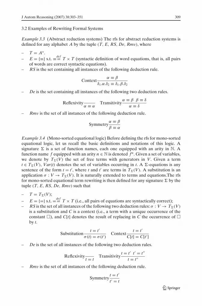
3.2 Examples of Rewriting Formal Systems

Example 3.3 (Abstract reduction systems) The rfs for abstract reduction systems isdefined for any alphabet A by the tuple (T, E, RS, De, Rmv), where

– T = A∗.– E = {≡} s.t. ≡def= T × T (syntactic definition of word equations, that is, all pairs

of words are correct syntactic equations).– RS is the set containing all instances of the following deduction rule.

Contextα ≡ β

δ1.α.δ2 ≡ δ1.β.δ2

– De is the set containing all instances of the following two deduction rules.

Reflexivityα ≡ α

Transitivityα ≡ β β ≡ δ

α ≡ δ

– Rmv is the set of all instances of the following deduction rule.

Symmetryα ≡ β

β ≡ α

Example 3.4 (Mono-sorted equational logic) Before defining the rfs for mono-sortedequational logic, let us recall the basic definitions and notations of this logic. Asignature is a set of function names, each one equipped with an arity in N. Afunction name f equipped with an arity n ∈ N is denoted f n. Given a set of variables,we denote by T(V) the set of free terms with generators in V. Given a termt ∈ T(V), Var(t) denotes the set of variables occurring in t. A -equations is anysentence of the form t = t′, where t and t′ are terms in T(V). A substitution is anapplication σ : V → T(V). It is naturally extended to terms and equations.The rfsfor mono-sorted equational term rewriting is then defined for any signature by thetuple (T, E, RS, De, Rmv) such that

– T = T(V);

– E = {=} s.t. =def= T × T (i.e., all pairs of equations are syntactically correct);– RS is the set of all instances of the following two deduction rules: σ : V → T(V)

is a substitution and C is a context (i.e., a term with a unique occurrence of theconstant �), and C[t] denotes the result of replacing in C the occurrence of �by t.

Substitutiont = t ′

σ(t) = σ(t ′)Context

t = t ′

C[t] = C[t ′]– De is the set of all instances of the following two deduction rules.

Reflexivityt = t

Transitivityt = t ′ t ′ = t ′′

t = t ′′


Symmetryt = t ′

t ′ = t


Example 3.5 (Conditional equational logic) The rfs developed in this example isthe logic that underlies the conditional rewriting to answer the validity problem ofunconditional equations. Only rewrite rules will have conditions.

Before defining this rfs let us recall some notions and notations of the conditionalequational logic. Signatures, terms with variables, and substitution are defined as inExample 3.4.

Atoms are -equations, and formulas are sentences of the form α1 ∧ . . . ∧ αn ⇒αn+1, where for every i, 1 ≤ i ≤ n + 1, αi is a -equation.

In order to make conditional formulas enter the definition of rfs that manipulatesonly predicates, any formula of the form c ⇒ t = t ′, where c =

∧

1≤i≤n

ti = t ′i (i.e., c is a

finite conjunction of equations), will be denoted by t =c t ′. Unconditioned equationst = t ′ will be denoted by t =∅ t ′. Hence, in the associated rfs, this gives rise to a familyof predicates =c indexed by finite conjunctions, and inference rules will be n-aryrelations on such formulas.

Therefore, given a signature , we define the rfs (T, E, RS, De, Rmv) for theconditional equational logic as follows:

– T = T(V);

– E = {=c | c : finite conjunction} s.t. for every c, =cdef= T × T (syntactic

definition);– RS is the set of all instances of the following deduction rule: Let σ : V → T(V)

be a substitution, and let C be a context

Replacement/Congruence

t = ∧

1≤i≤n

ti = t ′it ′ ∀1 ≤ i ≤ n, σ (ti) =∅ σ(t ′i)

C[σ(t)] =∅ C[σ(t ′)] .

– De is the set of all instances of the following two deduction rules.

Reflexivityt =∅ t

Transitivityt =∅ t ′ t ′ =∅ t ′′

t =∅ t ′′


Symmetryt =∅ t ′

t ′ =∅ t

Example 3.6 (Multisorted equational logic) For this rfs, a signature is a pair (S, F)

where S is a set of sorts and F is a set of function names, each one equipped with anarity in S∗ × S. A set of variable V = (Vs)s∈S is an S-indexed family of sets. Givena set of variables, we denote by T(V) = (T(V)s)s∈S the S-indexed family of setswhere, for every s ∈ S, T(V)s is the set of free terms of sort s with generators inV. -equations are any sentence of the form t = t ′ where there is s ∈ S such thatt and t ′ are terms in T(V)s. A substitution is an application σ : V → T(V) suchthat σ(Vs) ⊆ T(V)s. It is naturally extended to terms and equations. The rfs for


multisorted equational term rewriting is then defined for any signature by the tuple(T, E, RS, De, Rmv) such that

– T = T(V);

– E is the S-set of binary relations =s on T such that =sdef= T(V)s × T(V)s (all

pairs of terms define equations if both terms are of the same sort);– RS, De, and Rmv are defined as in Example 3.4.

Example 3.7 (Nonsymmetric transitive logic) The rfs for arbitrary (nonsymmetric)transitive relations is defined as in Example 3.4 except that E = {�} such that

�def= T × T. Moreover, we assume that every function f n is monotonic on allits positions with respect to �; that is, ∀1 ≤ i ≤ n, ti � t ′i ⇒ f (t1, . . . , ti, . . . , tn) �f (t1, . . . , t ′i, . . . , tn).8 Therefore, the deductive rules are as follows.

– RS is the set of all instances of the two following deduction rules: σ : V → T(V)

is a substitution, and C is a context

Substitutiont � t ′

σ(t) � σ(t ′)Monotonicity

t � t ′

C[t] � C[t ′] .

– De is the set of all instances of both of the following deduction rules.

Reflexivityt � t

Transitivityt � t ′ t ′ � t ′′

t � t ′′

– Rmv = ∅.

4 Rewrite Systems

4.1 Basic Definition

Rewriting orients binary predicates. We briefly saw in the introduction of thispaper that for any symmetric relation p, one rewriting relation suffices because→p= (←p)

−1, but for any nonsymmetric transitive one, two are needed. This wasfirst observed by J. Levy and J. Agustí and gave rise to bi-rewrite systems [32]. Inour generalization, since binary predicates in E are not necessarily symmetric, wefollow [32] and define rewrite systems as follows.

Definition 4.1 (Rewrite systems) Let S P = (T, E, RS, De, Rmv) be an rfs. AnS P-rewrite systems R is an E-sorted set of pairs of binary relations (→p,←p)p∈E

on T such that: ∀p ∈ E, →p ∪ ←p⊆ p (compatibility with the syntactic definitionof p given in S P).

8Otherwise, some restrictions need to be put on the context rule (called “Monotonicity” in thisexample and given below).


Example 4.2 In the rfs for abstract reduction systems, we can consider the followingset of rules from the alphabet A={a, b , c, . . . , z} ∪ {<, true, f alse}, which defines thelexicographic order: if ε denotes the empty word, then for every α and every β in A∗

ε < α →≡ truea < τ →≡ true with τ ∈ {b , c, d, . . . , z}

b < τ →≡ true with τ ∈ {c, d, . . . , z}...

y < z →≡ trueα < ε →≡ f alse

τ < a →≡ f alse with τ ∈ {b , c, d, . . . , z}τ < b →≡ f alse with τ ∈ {c, d, . . . , z}

...

z < y →≡ f alseτ.α < τ.β →≡ α < β with τ ∈ {a, b , . . . , z}

τ.α < τ ′.β →≡ τ < τ ′ with τ = τ ′ ∈ {a, b , . . . , z}

Because ≡ is symmetric, ←≡ is not considered here.

Example 4.3 In the rfs for mono-sorted equational logic, we can consider the fol-lowing set of rules from the signature = ({00, s1,+2,×2}, {x, y}), which definesarithmetic.

x + 0 →= x

x + s(y) →= s(x + y)

x × 0 →= 0

x × s(y) →= x × y + x

Because = is symmetric, ←= is not considered here.

Example 4.4 In the rfs developed for the conditional equational logic, we canconsider the following set of rules from the signature

= (true0, f alse0, 00, eq?2, _ mod _2, gcd2),

which specifies the greatest common divisor: to improve rule readability, throughoutthe paper we will write →c, →c

R and∗→c

R rather than →=c , →=cR and

∗→=c

R .

gcd(n, m) →eq?(n mod m,0)=true m

gcd(n, m) →eq?(n mod m,0)= f alse gcd(m, n mod m)

As in the two previous examples, because for every condition c,=c is symmetric,←=c

is not considered here.


Example 4.5 In the rfs for nonsymmetric transitive rewriting where ⊆ denotes theset-theoretical inclusion, we can consider the following set of rules from the signature = {∪2}, which defines the inclusion theory of union [32].

X ∪ X →⊆ X

X ←⊆ X ∪ Y

Y ←⊆ X ∪ Y

4.2 Rewriting Steps and Rewritings

We could be tempted to define rewriting steps and rewritings as the closures of binaryrelations →p and ←p under RS’s and De’s rule instances, respectively, that is, byorienting the conclusion of RS’s and De’s rule instances in the same direction as alltheir premises (this is how the standard rewriting relation is built in the uncondi-tioned equational rewriting setting). But many deduction rules do not satisfy sucha condition. For instance, this is not observed by the rule Replacement/Congruencegiven in Example 3.5. Indeed, when dealing with conditional rewrite rules, we have(at least) three potentially interesting definitions of →∅

R:9 natural, join, and normalrewriting. They were proposed in [20].10 Hence,→∅

R can be defined as follows: Givena rewrite system R = (→c)c:conjunction, let us define � = {t =c t ′ | t →c t ′ ∈ R}

1. Natural conditional rewriting C[σ(t)] →∅R C[σ(t ′)] if t →∧

1≤i≤nti = t ′it ′ ∈ R and for every

i, 1 ≤ i ≤ n, � � σ(ti) =∅ σ(t ′i),2. Join conditional rewriting C[σ(t)] →∅

R C[σ(t ′)] if t →∧

1≤i≤nti = t ′it ′ ∈ R and for every i,

1 ≤ i ≤ n, σ(ti) ↓∅ σ(t ′i), where ↓∅ means there is a term t ′′ such that σ(ti)∗→∅

R

t ′′ ∅R∗← σ(t ′i), or

3. Normal conditional rewriting C[σ(t)] →∅R C[σ(t ′)] if t →∧

1≤i≤nti = t ′it ′ ∈ R and for every

i, 1 ≤ i ≤ n, σ(ti)∗→∅

R σ(t ′i)

We observe that in the three cases, the orientation of the conclusion C[σ(t)] =∅C[σ(t ′)] of the Replacement/Congruence rule depends only on the orientation oft = ∧

1≤i≤nti = t ′it ′ in R. A similar phenomenon occurs in M. Schorlemmer’s logic of special

relations (see Section 9 in [1]).

9Other rewriting relations of the form →cR with c = ∅ are not considered because they are restricted

simply to rewrite rules (i.e., →cR=→c). Indeed, the rfs defined in Example 3.4 is the logical setting

that parameterizes classic conditional rewriting. But, the classic conditional rewriting was defined toanswer the validity problem of unconditioned equations (the conclusions of all deduction rules areof the form t =∅ t ′). Only rewrite rules are with conditions.10We can also cite [30] for the natural rewriting and [14, 15] for the join rewriting.


It then becomes obvious that some premises of rule instances have a special status.For any rule instance ι ∈ RS ∪ De, we gather its “special” premises in the multisetF L(ι) ⊆ L (ι) and call them fixed leaves. A sensible constraint is that F L(ι) is non-empty. The definition of these fixed leaves are ad hoc for each rfs. Therefore, givena deduction rule in RS ∪ De, the orientation of its conclusion will be influenced onlyby the orientation of its fixed leaves. In the next definition, we define in the abstractframework, both natural and normal rewritings. Join rewriting can also be abstractlydefined, but before that we need to give an abstract meaning of the notion of valleys,which will be done in Section 5.

Definition 4.6 (Rewriting step and rewriting relations) Let R be an S P-rewritesystem. For every p ∈ E, →p

R and∗→p

R are two binary relations on T defined as theleast binary relations (according to set-theoretical inclusion) inductively defined asfollows:

1. →p⊆→pR and →p

R⊆∗→p

R, and2. For every ι : p(t, t ′) ∈ RS (resp. ι : p(t, t ′) ∈ De) such that

– For every leaf p′(u, v) ∈ FL (ι), u →p′R v (resp. u

∗→p′

R v), and– For every leaf p′(u′, v′) ∈ L (ι) \FL (ι),

(a) Natural rewriting � � p′(u′, v′), where � = {p(t, t ′) | t →p t ′ ∈ R ∨t ←p t ′ ∈ R}

(b) Normal rewriting u′ ∗→p′

R v′ or u′ ∗←p′

R v′

we have t →pR t ′ (resp. t

∗→p

R t ′).

We denote by →R=⋃

p∈E

→pR and

∗→R=⋃

p∈E

∗→p

R. ←R=⋃

p∈E

←pR and

∗←R=⋃

p∈E

∗←p

R are defined analogously.

Remark 4.7 The two relations∗→R and

∗←R should not be confused with thereflexive and transitive closures of →R and ←R. There are only the closures of →R

and ←R under rules in De.

Example 4.8 In the abstract reduction system setting, a rewrite system R is givenby any binary relation →≡ on A∗. Moreover, all the premises of each instance ι ofboth deductive rules Context and Transitivity belong to FL (ι). Therefore, followingDefinition 4.6, →≡

R is the least binary relation on A∗ satisfying the following clauses:

– →≡⊆→≡R;

– If α →≡R β, then for every (δ1, δ2) ∈ A∗ × A∗, δ1.α.δ2 →≡

R δ1.β.δ2.

∗→≡R is then the reflexive and transitive closure of →≡

R. 11

11The symmetric closure of∗→≡

R is usually called Thue congruence.


Example 4.9 In the setting of mono-sorted equational rewriting, a rewrite system Ris given by any binary relation →= on T(V). Moreover, all the premises of eachinstance ι of the three deductive rules Substitution, Context, and Transitivity belongto FL (ι). Therefore, following Definition 4.6, →=

R is the least binary relation onT(V) satisfying the following clauses:

– →=⊆→=R;

– If t →=R t ′, then σ(t) →=

R σ(t ′), where σ : V → T(V) is any substitution;– If t →=

R t ′, then C[t] →=R C[t ′], where C is a context.

∗→=R is then the reflexive and transitive closure of →=

R.

Example 4.10 In the classic conditional rewriting setting, a rewrite system R is givenby a family of binary relations →c (c being a finite conjunction of equations) on

T(V). Moreover, for every instance ι

t= ∧

1≤i≤nti = t ′i

t ′ ∀1≤i≤n, σ (ti)=∅σ(t ′i)

C[σ(t)]=∅C[σ(t ′)] of the deductive

rule Replacement/Congruence, the set of its fixed leaves is FL (ι) ={

t = ∧

1≤i≤n

ti = t ′i

t ′}

. All the premises of every instance ι of the deductive rule Transitivity belong to

FL (ι). Therefore, following Definition 4.6, for every finite conjunction of equationsc = ∅, →c

R=→c, and →∅R is the least binary relation on T(V) satisfying the

following clause.

s →∅R t ⇔

⎧

⎪⎨

⎪⎩

∃l → ∧

1≤i≤nli = ri

r ∈ R, ω, σ,

s|ω = σ(l) ∧ t = s[σ(r)]ω ∧∧

1≤i≤n

σ(li) ∼ σ(ri)

In the natural and normal rewritings, ∼ is∗↔∅

R and∗→∅

R, respectively, where∗↔∅

R

and∗→∅

R are the reflexive, symmetric, and transitive closure and the reflexive andtransitive closure of →∅

R.

Example 4.11 In the setting of multisorted equational rewriting, a rewrite systemR is given by an S-indexed family of binary relations →=s on T(V)s with s ∈ S.Moreover, all the premises of each instance ι of the three deductive rules Substitution,Context and Transitivity belong to FL (ι). Therefore, following Definition 4.6, forevery s ∈ S→=s

R is the least binary relation on T(V)s satisfying the following clauses:

– →=s⊆→=sR ;

– If t →=sR t ′ then σ(t) →=s

R σ(t ′), where σ : V → T(V) is any substitution;– If t →=s

R t ′ then C[t] →=sR C[t ′], where C is a context.

For every s ∈ S,∗→=s

R is then the reflexive and transitive closure of →=sR .

Example 4.12 In the setting of nonsymmetric transitive rewriting, a rewrite systemR is given by two binary relations on T(V), →� and ←�, respectively. Therefore,


following Definition 4.6, →�R and ←�

R are both least binary relations on T(V)

satisfying the following clauses:– →�⊆→�

R and ←�⊆←�R;

– If t →�R t ′ (resp. t ←�

R t ′), then σ(t) →�R σ(t ′) (resp. σ(t) ←�

R σ(t ′)), where σ :V → T(V) is any substitution;

– If t →�R t ′ (resp. t ←�

R t ′), then C[t] →�R C[t ′] (resp. C[t] ←�

R C[t ′]), where C isa context.

∗→�R and

∗←�R are then the reflexive and transitive closures of →�

R and ←�R,

respectively.

Definition 4.13 (Convertibility relation) With all the notations of Definition 4.6,we denote by ↔R=

⋃

p∈E

↔pR, where for every p, ↔p

R is the least binary relation

satisfying: t ↔pR t ′ iff either t →p t ′ or t ←p t ′ or there exists ι : p(t, t ′) ∈ RS such

that

– For every p′(u, v) ∈ FL (ι), u ↔p′R v

– For every p′(u, v) ∈ L (ι) \FL (ι), u∗↔p′

R v.

Finally, we denote by∗↔R=

⋃

p∈E

∗↔p

R the closure of ↔pR under trees of De and Rmv;

that is, t∗↔p

R t ′ iff either t ↔pR t ′ or there exists ι : p(t, t ′) ∈ De ∪ Rmv such that

∀p′(u, v) ∈ L (ι), u∗↔p′

R v.∗↔R is called convertibility relation.

Remark 4.14 The relation∗↔R should not be confused with the reflexive and transi-

tive closure of ↔R. It is the closure of ↔R only under rules in De and Rmv.

From Definition 4.13, the convertibility relation∗↔R defines proof strategies that

restrict the proof search space by selecting proof trees equipped with the followingstructure: RS’s rule instances are always above both De’s rule instances and Rmv’srule instances. Let us call such proof trees rewrite trees. We must check that deriv-ability (i.e., syntactic consequences obtained from �) coincides with convertibility inrewriting, This property, named logicality,12 is expressed by � � p(t, t ′) ⇔ t

∗↔p

R t ′(� = {p(u, v) | u →p v ∈ R ∨ u ←p v ∈ R}).

Obviously, we have t∗↔p

R t ′ ⇒ � � p(t, t ′) because the convertibility relationdefines rewrite proofs that are peculiar proof trees. The other direction is moredifficult to prove because it requires that all statements of the form � � p(t, t ′) acceptsome rewrite proofs as proof trees. In all logics where the logicality result holds, thisis checked thanks to basic proof tree transformations that transform proof trees ofthe form (ι1, . . . , ιn, ϕ)ι such that

– ι ∈ RS,– ∃i, 1 ≤ i ≤ n, ιi ∈ De,– ∀i, 1 ≤ i ≤ n, ιi ∈ F ∪ R

12In the equational logic setting, this result is the so-called Birkhoff’s theorem.


into a rewrite tree π : ϕ. For instance, in the equational logic, we have the followingtransformation.

SubstTrans t=t ′ t ′=t ′′

t=t ′′σ(t)=σ(t ′′) � Trans

Subst t=t ′σ(t)=σ(t ′) Subst t ′=t ′′

σ(t ′)=σ(t ′′)σ (t)=σ(t ′′)

The difficulty is to show that the induced global proof tree transformation isnormalizing. In [3], we have provided a general setting under which results ofnormalization of proof trees, such as the logicality result in equational reasoningand the cut-elimination property in sequent or natural deduction calculi, can beunified and generalized. This has been achieved by giving simple conditions that aresufficient to ensure that such normalization results hold. These conditions are basedon basic properties of elementary combinations of inference rules that assure thatthe induced “global” proof tree transformation processes do terminate. We refer thereader to terms of this generalized version of the logicality theorem as well as itsproof in [2, 3]. Here, we postulate that convertibility coincides with deductions, thatis, � � p(t, t ′) ⇔ t

∗↔p

R t ′.

4.3 Derivations and Proofs

In the equational and nonsymmetric transitive rewriting setting, derivations andproofs can be simply defined by a sequence of rewriting steps. The transitivityapplication order on this sequence does not matter: different orders always end inthe same conclusion. This comes from the fact that transitivity instances can permutewith each other.

t1 r t2 t2 r t3t1 r t3

t3 r t4t1 r t4

�t1 r t2

t2 r t3 t3 r t4t2 r t4

t1 r t4r ∈ {≡,�,=,=∅}

Notice that both trees can be represented by the same sequence t1 r t2 r t3 r t4.In our generalization, we cannot define derivations and proofs as sequences of

rewriting steps because the applications of rule instances in De do not permutewith each other a priori. This situation leads us to denote them by trees. Hence, aderivation is a rewrite tree whose internal nodes and leaves are labeled by elementsof

∗→R (resp.∗←R) and →R (resp. ←R), respectively. Formally, this is defined as

follows.

Notation 4.15 Let us note t �pR t ′ and t

∗�

p

R t ′ to mean either t →pR t ′ or t ←p

R t ′,and t

∗→p

R t ′ or t∗←p

R t ′, respectively.

Remark 4.16 In any case, t �pR t ′ should not be confused with t ↔p

R t ′. In the firstcase, rewriting direction does not matter, but it exists. In the second case, we haveclosed →p

R under rule instances in Rmv.


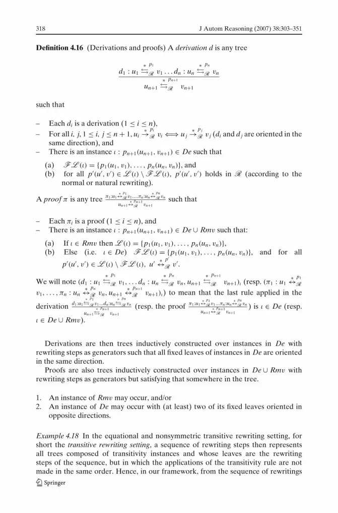
Definition 4.16 (Derivations and proofs) A derivation d is any tree

d1 : u1

∗�

p1

R v1 . . . dn : un

∗�

pn

R vn

un+1

∗�

pn+1

R vn+1

such that

– Each di is a derivation (1 ≤ i ≤ n),– For all i, j, 1 ≤ i, j ≤ n + 1, ui

∗→pi

R vi ⇐⇒ u j∗→p j

R v j (di and d j are oriented in thesame direction), and

– There is an instance ι : pn+1(un+1, vn+1) ∈ De such that

(a) FL (ι) = {p1(u1, v1), . . . , pn(un, vn)}, and(b) for all p′(u′, v′) ∈ L (ι) \FL (ι), p′(u′, v′) holds in R (according to the

normal or natural rewriting).

A proof π is any tree π1:u1∗↔p1

Rv1,...πn:un∗↔pn

Rvn

un+1∗↔pn+1

R vn+1

such that

– Each πi is a proof (1 ≤ i ≤ n), and– There is an instance ι : pn+1(un+1, vn+1) ∈ De ∪ Rmv such that:

(a) If ι ∈ Rmv then L (ι) = {p1(u1, v1), . . . , pn(un, vn)},(b) Else (i.e. ι ∈ De) FL (ι) = {p1(u1, v1), . . . , pn(un, vn)}, and for all

p′(u′, v′) ∈ L (ι) \FL (ι), u′ ∗↔p′

R v′.

We will note (d1 : u1

∗�

p1

R v1, . . . dn : un

∗�

pn

R vn, un+1

∗�

pn+1

R vn+1)ι (resp. (π1 : u1∗↔p1

R

v1, . . . , πn : un∗↔pn

R vn, un+1∗↔pn+1

R vn+1)ι) to mean that the last rule applied in the

derivation d1:u1

∗�

p1

Rv1...dn:un

∗�

pn

Rvn

un+1

∗�

pn+1

R vn+1

(resp. the proof π1:u1∗↔p1

Rv1...πn:un∗↔pn

Rvn

un+1∗↔pn+1

R vn+1

) is ι ∈ De (resp.

ι ∈ De ∪ Rmv).

Derivations are then trees inductively constructed over instances in De withrewriting steps as generators such that all fixed leaves of instances in De are orientedin the same direction.

Proofs are also trees inductively constructed over instances in De ∪ Rmv withrewriting steps as generators but satisfying that somewhere in the tree.

1. An instance of Rmv may occur, and/or2. An instance of De may occur with (at least) two of its fixed leaves oriented in

opposite directions.

Example 4.18 In the equational and nonsymmetric transitive rewriting setting, forshort the transitive rewriting setting, a sequence of rewriting steps then representsall trees composed of transitivity instances and whose leaves are the rewritingsteps of the sequence, but in which the applications of the transitivity rule are notmade in the same order. Hence, in our framework, from the sequence of rewritings


t1 →=R t2 →=

R . . . →=R tn, many derivations can be considered such as for instance the

application of the transitivity rule from left to right:

d1

d0 t1→=Rt2

d′0 t2→=Rt3

t1∗→=

R t3 d′1 t3→=Rt4d2

t1∗→=

R t4...

dn−3......

t1∗→=

Rtn−1

d′n−3 tn−1→=Rtn

dn−2

t1∗→=

R tnHere, for each i, 1 ≤ i ≤ n − 2, each derivation di is denoted by (di−1 : t1

∗→=R

ti+1, d′i−1 : ti+1 →=R ti+2, t1

∗→=R ti+2) t1=ti+1 ti+1=ti+2

t1=ti+2

.

In the nonsymmetric but transitive rewriting setting, because the transitivity ruleis of the form t�t ′ t ′�t ′′

t�t ′′ , sequences of rewriting are

– Either of the form t1 →�R t2 →�

R t3 . . . →�R tn,

– Or tn ←�R tn−1 ←�

R tn−2 . . . ←�R t1, that is t1

�R → t2

�R → t3 . . .

�R → tn.

Therefore, by applying the transitivity rule from left to right, for instance, we haveboth following derivations.

1.

d1

d0 t1→�Rt2

d′0 t2→�Rt3

t1∗→�

R t3 d′1 t3→�Rt4d2

t1∗→�

R t4...

dn−3...

t1∗→�

Rtn−1

d′n−3 tn−1→�Rtn

dn−2

t1∗→�

R tn

2.

d1

d0 t1�R→t2

d′0 t2�R→t3

t1�R

∗→ t3 d′1 t3�R→t4d2

t1�R

∗→ t4...

dn−3...

t1�R

∗→tn−1

d′n−3 tn−1�R→tn

dn−2

t1�R

∗→ tn

As an example of proof, let us consider the following sequence of term rewriting:

t1 →=R t2 =

R ← t3 =R ← t4 →=

R t5 =R ← t6 →=

R t7.


The following trees are examples of proofs that are the results of differentapplication orders of transitivity on the above sequence.

d00 : t1 →=

R t2 d10 : t2

=R ← t3

d01

t1∗↔=

R t3

d20 : t3

=R ← t4 d3

0 : t4 →=R t5

d11

t3∗↔=

R t4d0

2t1

∗↔=R t5

d21 : t5

=R ← t6 d3

1 : t6 →=R t7

d12

t5∗↔=

R t7d3

t1∗↔=

R t7

d02 : t1 →=

R t2

d00 : t2

=R ← t3 d1

0 : t3=R ← t4

d01

t2=R

∗← t4d1

1 : t4 →=R t5

d12

t2∗↔=

R t5d0

3t1

∗↔=R t5

d22 : t5

=R ← t6 d3

2 : t6 →=R t7

d13

t5∗↔=

R t7d4

t1∗↔=

R t7

d00 : t1 →=

R t2 d10 : t2

=R ← t3

d01

t1∗↔=

R t3d1

1 : t3=R ← t5

d02

t1∗↔=

R t4d1

2 : t4 →=R t5

t1∗↔=

R t5

d22 : t5

=R ← t6 d3

2 : t6 →=R t7

d13

t5∗↔=

R t7d4

t1∗↔=

R t7

5 Properties of Rewrite Systems

In the transitive rewriting setting, rewrite systems are used to answer the validityproblem of theories when they are both confluent and terminating, that is, convergent.To define convergent rewrite systems in our framework, we must then give anabstract formulation of termination and confluence.

5.1 Termination

A naive approach to define the termination of rewrite systems would be that deriva-tions cannot be expanded indefinitely, expansion of derivations meaning that someother derivations contain them as subtrees. Of course, this condition is sufficient butis too weak. Indeed, in the equational rewriting setting, the instantiation of such adefinition would be as follows: A rewrite system is terminating if every derivationt1 → t2 → . . . → tn is

– Unexpandable to the right t1 → t2 → . . . → tn →tn+1

– Unexpandable to the left t0 →t1 → t2 → . . . → tn.

Condition 1 is the right one, which is usually taken into account to definetermination of rewrite systems. On the contrary, Condition 2 cannot be imposed;otherwise most classic rewrite systems would be considered as unterminating, whichwould be counterintuitive.

In our generalization, expansion to the left or to the right has no meaning becausethe algebraic structures under consideration are not necessarily transitive. We then


have to denote derivations by trees (see the previous section). Therefore, we haveto define a similar notion to the notion of expanding to the left and to the rightbut for trees. This is obtained by associating for every ι = p1(u1,v1)...pn(un,vn)

p(u,v)in De

a number i, 1 ≤ i ≤ n, such that pi(ui, vi) ∈ FL (ι), which denotes the positionamong the premises of ι where derivations are to be expanded. We will denote this

position by→E x (ι) (resp.

←E x (ι)). For instance, in the equational rewriting setting, for

every transitivity instance ι = u=v v=wu=w

,→E x (ι) = 1 (

←E x (ι) is not considered because

equalities are symmetric). Hence, if we consider the derivation d : u∗→=

R v, any

expansion of d from ι has necessarily the following form d:u ∗→=Rv d′ :v ∗→=

Rw

u∗→=

Rw. From such

an expanding position, we can define an expanding relation ER on derivations asfollows.

d : u∗→=

R v ERd : u

∗→=R v d′ : v ∗→=

R w

u∗→=

R w

Let us also denote by ER the transitive closure of this expanding relation. Therefore,in the equational rewriting setting, we can redefine the termination of rewrite systemsas follows: a rewrite system is terminating if and only if ER is Nœtherian.13

Because ER has been defined on derivations denoted by trees, it can be general-ized in our abstract framework as follows:

Definition 5.1 (Expanding positions and expanding relation) Let S P be an rfs.

Expanding positions are defined by two applications→E x,

←E x: De → N satisfying for

every ι = p1(u1,v1)...pn(un,vn)

p(t,t ′) in De:

–→E x (ι) =

←E x (ι),

– 1 ≤→E x (ι) ≤ n and 1 ≤

←E x (ι) ≤ n, and

– If j =→E x (ι) and k =

←E x (ι) then pj(u j, v j) and pk(uk, vk) belong to FL (ι).

Let R be an S P-rewrite system. Let us denote by ER the binary relation onderivations defined as the transitive closure of

d : u∗→p′

R v ER (d′ = (d1, . . . , dm, t∗→p

R t ′)ι) ⇐⇒ d →E x(ι)

= d

d : u∗←p′

R v ER (d′ = (d1, . . . , dm, t∗←p

R t ′)ι) ⇐⇒ d ←E x(ι)

= d.

Example 5.2 The symmetric and transitive rewriting setting has already been han-dled above. In the nonsymmetric transitive rewriting setting, both expanding posi-

tions for every instance ι of the transitivity are respectively,→E x (ι) = 1 and

←E x (ι)=2.

13A Nœtherian relation is not necessarily irreflexive. A reflexive binary relation can be Nœtherianprovided that all infinite ordered sequences are stationary, that is, there is a position i ∈ N from whichthe following elements in the sequence are equal.


Therefore, the expanding relation for any S P-rewrite system R is defined as shownin the figure below.

Let us observe that ER induces a partition of derivations; that is, if d ER d′, then dand d′ have their conclusions that are oriented in the same direction.

Although defining termination from Nœtherianess of ER is sufficient for bothequational and conditional rewriting settings, this is too weak for the nonsymmetrictransitive one. Indeed, in such a rewriting setting, this would be equivalent to

imposing that both∗→�

R and �R

∗→ are Nœtherian orderings.14 However, it has beenshown in [32] that this is a weaker condition not sufficient to have Newman’s lemma(i.e., the equivalence between the Church–Rosser and local confluence propertiesunder termination of rewrite systems). To obtain such a result, we have to definethe termination of rewrite systems by the following: (→�

R ∪ �R→)∗ is a Nœtherian

ordering. This motivates the concept of reduction relation, that is, a binary relationthat is known to be terminating and embodies in its definition the closure propertiesunder instances in RS and De. Moreover, proving termination of a rewrite systemoften requires checking an infinite set of expansions of each derivation in R. A wayto answer this problem is also to use the concept of reduction relation as is stemmedfrom Theorem 5.7 below. Here, as previously, reduction relations are not necessarilyorders.

Definition 5.3 (Reduction relation) Let S P = (T, E, RS, De, Rmv) be an rfs

equipped with both expanding position applications→E x and

←E x. A rewriting relation

� is an E-indexed family of binary relations �p on T satisfying for each p ∈ E:

– �p⊆ p ∪ p−1,– �p is closed under instances in RS and De (cf. Definition 4.6).

14This is because two derivations d and d′ satisfying d ER d′ have their conclusions that are orientedin the same direction.


A reduction is any tree resulting from the inductive construction of �, that is, anytree r = r1:u1�p1 v1...rn:un�pn vn

un+1�pn+1 vn+1such that

– Each ri is a reduction (1 ≤ i ≤ n), and– There is an instance ι : pn+1(un+1, vn+1) ∈ De or ι : pn+1(vn+1, un+1) ∈ De such

that

(a) For all i, 1 ≤ i ≤ n, pi(ui, vi) ∈ FL (ι) or pi(vi, ui) ∈ FL (ι), and(b) For all p′(u′, v′) ∈ L (ι) \FL (ι), we have either u′ �p′ v′ or v′ �p′ u′.

As for derivations, we can define an expanding relation E� on reductions accord-

ing to→E x, that is,

r : u � v E� (r′ = (r1, . . . , rm, t � t ′)ι) ⇐⇒ r →E x(ι)

= r.

Therefore, a reduction relation is any rewriting relation � such that its expandingrelation E� is Nœtherian.

Example 5.4 In the abstract reduction system rewriting, a reduction relation is anywell-founded order stable under context. In both mono-sorted and multisortedrewriting settings, a reduction relation is any well-founded order stable under contextand substitution. In the conditional rewriting setting, a reduction relation is a familyof well-founded binary relations �c (c:finite conjunction of equations) such that �∅ isan order stable under replacement/congruence, that is if u � ∧

1≤i≤nti = t ′i v and for every

i, 1 ≤ i ≤ n, we have either ti �∅ t ′i or t ′i �∅ ti, then, u �∅ v.To benefit from all classic methods that facilitate proof of termination such as

reduction and simplification orders, we can establish that for every finite (possiblyempty) conjunction c, �c=> where > is a well-founded ordering on terms stableunder substitution and context. This is compatible with the definition of reductionrelations such as proposed in this paper. Indeed, �=

⋃

c

�c => is obviously stable

under replacement/congruence.Finally, in the setting of nonsymmetric transitive rewriting, a reduction relation is

any well-founded order monotonic and stable under substitution.

Termination of rewrite systems is then defined as follows:

Definition 5.5 (Termination of rewrite systems) Let R be an S P-rewrite system.Let us define, for every p ∈ E, �p

R= (→p ∪(←p)−1)∗ ((. . .)∗ meaning “closed under

instances in RS and De”). Obviously, �R= (�pR)p∈E is a rewriting relation. There-

fore, R is terminating if and only if �R is a reduction relation.

Example 5.6 In the equational rewriting setting, because →=R= (←=

R)−1, we have

�=R=

∗→=R and then E�R = ER. On the contrary, in the nonsymmetric transitive

rewriting setting, ��R= (→�

R ∪(←�R)−1)∗. Therefore, ER ⊆ E�R .

Theorem 5.7 An S P-rewrite system R is terminating if and only if there exists areduction relation � such that ∀p ∈ E, →p ∪(←p)

−1 ⊆�.


Proof If R is terminating, set �=�R. Conversely, we have E�R ⊆ E�. As E� isNœtherian, so is E�R . �

In the term equational rewriting setting, this last theorem was established byLankford [31] (see [5], p. 103, for the statement of this theorem). Here, Theorem 5.7is a generalized form of this result.

5.2 Generalized Form of Church–Rosser and Confluence Properties

From Definition 4.17, proofs are composed of derivations connected together via ruleinstances in De ∪ Rmv. Therefore, among proofs we have derivations as well as allproofs composed of derivations connected together via one instance of a rule in Dewith some orientation conflicts on fixed leaves. Let us call such proofs basic proofs.They are defined as follows.

Definition 5.8 (Basic proofs) A basic proof is either a derivation or a proof π of theform (d1, . . . , dn, u

∗↔p

R v)ι with ι ∈ De and for every i, 1 ≤ i ≤ n, di is a derivation.Let us denote by BP the set of basic proofs.

Example 5.9 In the equational rewriting setting, basic proofs are elements of(∗→ ◦ ∗←) ∪ (

∗← ◦ ∗→); that is, a basic proof is a proof that has one of the two followingforms.

1.d1 : u

∗←=R w d2 : w ∗→=

R v

u∗↔=

R v, or

2.d1 : u

∗→=R w d2 : w ∗←=

R v

u∗↔=

R v

In the nonsymmetric transitive rewriting setting, basic proofs are elements in

(∗→�

R ◦ ∗←�R) ∪ (

∗←�R ◦ ∗→�

R), that is, a basic proof is a proof that has one of the twofollowing forms.

1.d1 : u

∗←�R w d2 : w ∗→�

R v

u∗↔�

R v, or

2.d1 : u

∗→�R w d2 : w ∗←�

R v

u∗↔�

R v

Obviously, proofs are then basic proofs connected together via a finite set ofrule instances in De ∪ Rmv. In order to reduce the proof search space when we wantto establish that two elements are convertible, the adopted strategy is to replacesome basic proof trees, called in this paper effluences, by other ones, called hereproofs by rewriting. This is Church–Rosser’s result, which we will generalize innext section. When all effluences can be replaced by proofs by rewriting for anS P-rewrite system R, R is said to be confluent. In order to test automatically thisproperty, effluences have to be eliminated step by step by replacing local effluences,which are effluences whose derivations are restricted to rewriting steps (this is


a general form of Newman’s lemma that we will formally give and prove in thenext section).

Therefore, the generalization of the confluence property requires us first to dividebasic proofs into effluences and proofs by rewriting such that one must be able togenerate proofs by rewriting from the decision procedure used to answer the va-lidity problem of theories. Proofs by rewriting and effluences are then defined asfollows.

Definition 5.10 (Proof by rewriting and effluence) Proofs by rewriting and effluencesform a partition PR and E f f of BP (the set of basic proofs) such that for anyformula p(u, v), the set RS[p(u, v)] defined by

{u′ �R v′ | ∃(d1, . . . , dn, u∗↔p

R v) ∈ PR, ∃1 ≤ i ≤ n, u′ �R v′ ER di}is finite and computable; that is, we can construct the Turing machine capable oflisting all its members out of a given rewrite system.

A local effluence is an effluence of E f f of the form (u1 �R v1, . . . , un �R

vn, u∗↔R v).

Remark 5.11 Given a formula p(u, v), the set RS[p(u, v)] then contains all therewriting steps that start some proofs by rewriting with u

∗↔p

R as conclusion.

The condition of Definition 5.10 will be useful to define a decision procedure usedto answer the validity problem of theories (see the algorithm just below).

Example 5.12 In the equational rewriting setting, proofs by rewriting and effluencesare valleys and peaks, respectively. Following our notations, peaks and valleys aredefined as follows.

– A peak is any basic proof tree of the form d1:u ∗←=Rw d2:w ∗→=

Rv

u∗↔=

Rv

– A valley is either a derivation or any basic proof tree of the form d1:u ∗→=Rw d2:w ∗←=

Rv

u∗↔=

Rv

This partition satisfies the condition of Definition 5.10. Indeed, suppose an equationu = v. Then, let us define the set S as follows:

S =⎧

⎨

⎩

{u′ | u →=R u′}

∪{v′ | v →=

R v′}

For any derivation d : u+→=

R w15 there is a term u′ such that d = d1:u→=Ru′ d2:u′ ∗→

=Rw

u∗→=

Rw.

This means, by the definition of the expanding position application→E x, that d1 :

u →=R u′ ER d. Consequently, we have the following.

RS[u = v]⎧

⎨

⎩

{u →=R u′ | u′ ∈ S }

∪{v →=

R v′ | v′ ∈ S }

15Recall that+→R is the transitive closure of →R. Hence, u

+→=R w contains at least a rewriting step.


Moreover, for any rewrite system R with a finite set of rewriting rules, therewriting relation →R is decidable and finitely branching; that is, each term has onlyfinitely many direct successors that can be automatically listed. Therefore, RS[u = v]is finite and computable.

On the contrary, if proofs by rewriting were peaks and effluences were valleys,then for some u = v, the set RS[u = v] would not be necessarily finite anymore.Indeed, there could be an infinite set of terms t such that u

∗← t∗→ v.

Arguments and reasoning for the nonsymmetric transitive rewriting setting aresimilar.

But, when dealing with conditional rewriting, the set RS[u =c v] is not computablebecause →R is not decidable in general. Indeed, performing rewriting steps requiresto rewrite (join16 and normal rewriting) or to automatically satisfy (natural rewriting)the premises of rewriting rules. In the literature, some conditions such as “decreas-ingness” [19] have been proposed so that joinability and rewriting are decidable.

Now we can define the join rewriting that had been left in pending in the previoussection. This gives rise to the following definition.

Definition 5.13 (Join rewriting) Let R be an S P-rewrite system. For every p ∈ E,→p

R and∗→p

R are the least binary relations on T (according to the set-theoreticalinclusion) inductively defined as follows:

1. →p⊆→pR and →p

R⊆∗→p

R, and2. For every ι : p(t, t ′) ∈ RS (resp. ι : p(t, t ′) ∈ De) such that

– For every leaf p′(u, v) ∈ FL (ι), u →p′R v (resp. u

∗→p′

R v), and

– For every leaf p′(u′, v′) ∈ L (ι) \FL (ι), there is π : u′ ∗↔p′

R v′ ∈ PR,

we have t →pR t ′ (resp. t

∗→p

R t ′)

We define →R=⋃

p∈E

→pR and

∗→R=⋃

p∈E

∗→p

R. ←R=⋃

p∈E

←pR and

∗←R=⋃

p∈E

∗←p

R

are defined analogously.

In the following of this section, we will consider only join rewriting.In order to define a decision procedure from a given terminating rewrite system,

the expanding relation ER of any S P-rewrite system R must satisfy two supple-mentary properties.

1. Rewritings can be characterized by some derivations that can be generated stepby step.

2. When dealing with finite rewrite systems, the choice to extend derivations byrewriting steps is finite and computable; that is, we can construct the Turingmachine capable of listing all its members out of a given rewrite system.

16A generalization of such a rewriting is given in Definition 5.13.


Formally, this is expressed as follows.

Notation 5.14 Let us define�E x to mean either

→E x or

←E x.

Definition 5.15 (Sensible rewrite system) An S P-rewrite system R is sensible ifand only if its expanding relation ER satisfies both following properties.

1. Generated step by step: For any rewriting u∗�R v, there is a derivation d : u

∗�R

v and a finite sequence of derivations d1 ER . . .ER dn such that

– d = dn,– d1 : u1 �R v1 is a rewriting step, and

– For all i, 2 ≤ i ≤ n, di = (d′1, . . . , d′m, ui

∗�R vi)ι such that for every j, 1 ≤

j =�E x (ι) ≤ m, d′j is a rewriting step.

2. Finite and computable derivation extension choice: Let d be a derivation. Let usdenote by D[d] the set of derivations d′ satisfying the following properties:

– d ER d′, and

– d′ is of the form (d1, . . . , dn, ϕ)ι such that for every j, 1 ≤ j =�E x (ι) ≤ n, d j is

a rewriting step.

Then, for every derivation d, D[d] is finite and computable.

D[d] is the set of derivations that expand the derivation d by adding a rewritingstep.

Example 5.16 When dealing with transitive rewriting settings (i.e., both equationaland nonsymmetric transitive rewriting) for each rewriting t

∗→ t ′, since∗→ is transi-

tive, there exist n terms t1, . . . , tn such that

t → t1 t1 → t2

t∗→R t2 t2 → t3

t∗→R t3

. . . . . .

t∗→R tn tn → t ′

t∗→R t ′

.

Finally, given a derivation d : u∗→R v, we have seen in Example 5.12 that v can

be rewritten in one step, into a finite set of terms v′, that is, d ERd:u ∗→Rv d′ :v→Rv′

d:u ∗→Rv′.

Moreover, generating the set of terms v′ such that v →R v′ is a finite and computable

task. Therefore, D[d] defined as the set of derivations of the form d:u ∗→Rv d′ :v→Rv′

u∗→Rv′

is

also finite and computable.

Based on the sensible S P-rewrite system R = (→p,←p)p∈E, a decision pro-cedure for its corresponding theory Th(�) = {p(u, v) | � � p(u, v)}, where � =


{p(u, v) | u �p v ∈ R}, can be defined. To prove � � p(u, v), we perform thefollowing algorithm A on p(u, v), written A [p(u, v)].

Input a rewrite system R and a formula p(u, v).Initialization S := RS[p(u, v)], Tmp := RS[p(u, v)], and answer := f alse;Loop while Tmp = ∅ do:

1) choose d in Tmp and Tmp := Tmp \ {d};2) Tmp := Tmp ∪ D[d]; (cf. Definition 5.15)3) S := S ∪ Tmp;4) if there is (d1, . . . , dn, u

∗↔p

R v)ι ∈ PR such that:

– di ∈ S (1 ≤ i ≤ n), and– ∀p′(u′, v′) ∈ L (ι) \FL (ι), A [p′(u′, v′)]then Tmp := ∅;

answer := true;

end of loopOutput return(answer)

The above procedure calls for some comments:

– As assured by Point (4) in the algorithm, proofs generated by the above decisionprocedure are proofs by rewriting.

– The kind of rewriting that is taken into account by the above procedure is thejoin one. Indeed, as this is expressed by the second bullet under Item 4, we applythe algorithm A to each formula p′(u′, v′) ∈ L (ι) \FL (ι) with p′ ∈ E. Hence,

we try to find a proof by rewriting π : u′ ∗↔p′

R v′.

Example 5.17 When dealing with transitive relations, the direct instantiation of theabove procedure is as follows.

Initialization S := {d | ∃w, d : u →rR w ∨ d : w ←r

R v} and Tmp := {d | ∃w,

d : u →rR w ∨ d : w ←r

R v} with r ∈ {=,�}, and answer := f alse.Loop while Tmp = ∅ do:

1) choose d : a∗�

r

R b in Tmp and Tmp := Tmp \ {d};17

2) Tmp := Tmp ∪ {d′ : a∗�

r

R c | b �rR c ∧ (a

∗→r

R b ⇔ b →rR c)};18

3) S := S ∪ Tmp.4) if there are u

∗→r

R c and c∗←r

R v in S, then Tmp := ∅;answer := true;

end of loopOutput return(answer)

The above procedure defines a breadth-first search proof for the theory R.

17a is necessarily either u or v.18The last condition means that both rewritings are in the same direction.


Note that the above algorithm is recursive and hence can loop even when rewritesystems are terminating. Indeed, nothing prevents applying again A [p(u, v)] in theexecution of A [p′(u′, v′)]. A sufficient condition to prevent such a situation is thefollowing.

Definition 5.18 (Adequacy) Let S P be an rfs. Let !" be a binary relation onformulas defined by

p(u, v) !" p′(u′, v′) ⇐⇒ ∃ι : p(u, v) ∈ De, p′(u′, v′) ∈ L (ι) \FL (ι).

Therefore, S P is adequate if and only if the transitive closure !"+ of !" isNœtherian.

The intuition under Definition 5.18 is that in any proof π : u∗↔p

R v, there is no

subproof (π1, . . . , πn, u′ ∗↔p′

R v′)ι such that p(u, v) belongs to unfixed leaves of ι (i.e.,p(u, v) ∈ L (ι) \FL (ι)). Would such a subproof exist, solving p(u, v) by rewritingshould require to search a proof by rewriting π : u

∗↔p

R v and would then loop.This condition is obviously satisfied by all the examples developed up to here in

this paper because the set of unfixed leaves of transitivity instances is empty. Withconditional rewriting, undecidability problems of joinability have been relegated tothe level of the execution of rewriting steps (see Example 5.12).

Given an rfs S P = (T, E, RS, De, Rmv), its adequacy can be obviously checkedwhen the set E is finite and we are dealing with a finite set of inference rule schemas.

We are in a position to define properties of rewrite systems.

Definition 5.19 (Properties of rewrite systems) An S P-rewrite system R is

– Confluent (resp. locally confluent) if for any effluence (resp. local effluence) thereis an equivalent proof by rewriting, and

– Church–Rosser if for any proof there is an equivalent proof by rewriting.

For any adequate rfs S P , Church–Rosser and terminating rewrite systems canbe used to answer the validity problem as this is expressed by the following result.

Theorem 5.20 Let S P be an adequate rfs. If the S P-rewrite system R = (→,←) isChurch–Rosser, then � � p(u, v) if and only if the procedure defined above terminatesand answers true. Moreover, if R is Church–Rosser and terminates, then the validityproblem is decidable.

Proof Theorem 5.20 is composed of two properties. Let us prove the first one definedby the following equivalence:

� � p(u, v) (p ∈ E) if and only if the procedure defined above terminates andanswers true.

The if implication is easily proven from Point (4) of the procedure.By the generalized version of the logicality theorem established in [2], when

� � p(u, v), we have necessarily u∗↔p

R v. As R is Church–Rosser, then there is a

proof by rewriting π : u∗↔p

R v that establishes the statement � � p(u, v). Therefore,


let us prove the only if implication by induction with respect to the ordering!". Let π = (d1, . . . , dn, u

∗↔p

R v)ι be a proof by rewriting. From both constraintsrequiring that RS[p(u, v)] and D[d] are finite and computable for every derivationd, each derivation di (1 ≤ i ≤ n) will be generated in a finite time by the abovedecision procedure. Moreover, for every p′(u′, v′) ∈ L (ι) \FL (ι), by the inductionhypothesis, the decision procedure terminates and answers true. Therefore, π will begenerated in a finite time by the above decision procedure.

The second property is given by the following implication:

If R is Church–Rosser and terminates, then the validity problem is decidable.

As R is terminating and from all explanations given just before, given a formulap(u, v), the set of proofs by rewriting π : u

∗↔p

R v can be generated in a finite time,when they exist. Therefore, for any p(u, v), the algorithm answers in a finite time thatthe statement � � p(u, v) is true or not. �

6 Generalization of Church–Rosser’s Result and Newman’s Lemma

Congruences (defined by a set of equations), which are a typical example of algebraicstructure where rewriting has been intensively studied and applied, have a numberof (implicit) properties that are useful for rewriting but are not necessarily satisfiedin all rfs (as they are not required in Definition 3.1). In this section, we thusgive, by means of a set of axioms, the conditions needed for a rfs to satisfy theseuseful properties. First of all, Church–Rosser’s result establishes a correspondencebetween Church–Rosser systems and confluent systems. Obviously, Church–Rossersystems are confluent systems because effluences are peculiar proofs. The oppositeimplication is more difficult. In the transitive rewriting setting, this implication has adiagrammatic proof based on the two following observations.

1. Proofs can be written as a series of maximal peaks (i.e., peaks that are notcontained in another one).

2. Replacement of any maximal peak by a valley decreases the number of maximalpeaks.19

In all rewriting theories, these two basic requirements are behind all proofs ofChurch–Rosser’s result. Their abstraction requires first to give an abstract formula-tion of maximal peaks. This leads to the following definition.

Definition 6.1 (Maximal effluences) Let π : ϕ and π ′ : ϕ be two proofs with L (π) =L (π ′). Let w ∈ N∗ be a position such that π ′

|w is an effluence. The pair (π ′, w) isa maximal effluence of π if and only if no other pairs (π ′′, w′) satisfy the sameconditions as (π ′, w) and such that L (π ′

|w ) ⊂ L (π ′′|w′ ).

Let us denote NEM(π) the number of maximal effluences in π . The notationπ ≤em π ′ means that NEM(π) ≤ NEM(π ′).

19Actually, this number decreases of one unit.


Example 6.2 Let π be the tree obtained from the following rewriting sequence byapplying transitivity instances from left to right.

t1 → t2 ← t3 ← t4 → t5 ← t6 → t7

The following pairs are examples of effluences of π .

1.

⎛

⎜

⎜

⎜

⎜

⎜

⎜

⎝

t1 → t2 ← t3

t1∗↔ t3

t3 ← t4 → t5

t3∗↔ t5

t1∗↔ t5

t5 ← t6 → t7

t5∗↔ t7

t1∗↔ t7

, 0.1

⎞

⎟

⎟

⎟

⎟

⎟

⎟

⎠

2.

⎛

⎜

⎜

⎜

⎜

⎜

⎜

⎜

⎜

⎜

⎜

⎜

⎝

t1 → t2

t2 ← t3 ← t4

t2∗← t4 t4 → t5

t2∗↔ t5

t1∗↔ t5

t5 ← t6 → t7

t5∗↔ t7

t1∗↔ t7

, 0.1

⎞

⎟

⎟

⎟

⎟

⎟

⎟

⎟

⎟

⎟

⎟

⎟

⎠

3.

⎛

⎜

⎜

⎜

⎜

⎜

⎜

⎜

⎜

⎜

⎜

⎜

⎝

t1 → t2 ← t3

t1∗↔ t3 t3 ← t4

t1∗↔ t4 t4 → t5

t1∗↔ t5

t5 ← t6 → t7

t5∗↔ t7

t1∗↔ t7

, 1

⎞

⎟

⎟

⎟

⎟

⎟

⎟

⎟

⎟

⎟

⎟

⎟

⎠

But only the second and the third ones are maximal effluences of π (not the first onebecause {t3 ← t4, t4 → t5} is included in {t2 ← t3, t3 → t4, t4 → t5}).

Given a finite set S of rewriting steps, there will be a finite set (possibly empty) ofmaximal effluences with premises in S if we can only build a finite set of proofs fromS using rule instances in De. This will be our first postulate.

Axiom 1. Given a finite set S of rewriting steps, there exists a finite set of proofs π

only using rule instances in De and such that L (π) ⊆ S.

In our general setting, the first requirement above (i.e., writing proofs as a seriesof maximal peaks) holds only for any proof that does not contain instances of rulesin Rmv. This is a consequence of the fact that effluences and proofs by rewritingform a partition of all basic proofs. Hence, any proof without maximal effluencesor instances of rules in Rmv is necessarily a proof by rewriting. Therefore, to write


proofs as series of maximal peaks in our general setting, we must postulate that ruleinstances in Rmv are redundant.

Axiom 2. For any proof π : ϕ, there exists an equivalent proof π ′ : ϕ using onlyrule instances in De.

Example 6.3 In the equational rewriting setting, Axiom 2 obviously holds. Indeed,for every u

∗→R w∗←R v and every u

∗←R w∗→R v, we also have v

∗→R w∗←R u

and v∗←R w

∗→R u.In the nonsymmetric transitive rewriting setting, Axiom 2 is meaningless because

Rmv is empty.

Hence, for every rewrite system R that satisfies Axioms 1 and 2, we can restrictour attention to proofs only built from rule instances in De. The consequence is inthis case, for every proof π , NEM(π) belongs to N.

In our general setting, the second requirement (i.e., replacing a maximal proofin a proof by a rewriting proof decreases the number of maximal proofs) does notnecessarily hold. Therefore, it has to be imposed.

Axiom 3 (Cut in maximal effluences). For any proof π , the replacement of one of itsmaximal effluences (π ′, w) by an equivalent proof by rewriting π ′′ (i.e., with the sameconclusion as π ′|w ) decreases the number of maximal effluences: π ′[π ′′]w <em π ′.

Example 6.4 In the transitive rewriting setting, Axiom 3 holds. Indeed, we sawpreviously that proofs can be written as a series of maximal peaks. It is clear thatthe replacement of any maximal peak by a valley reduces by one unit the number ofmaximal peaks.

Axioms 1–3 induce Church–Rosser’s result.

Theorem 6.5 (Generalized Church–Rosser’s result) For every rewrite system R forwhich Axioms 1–3 hold, R is Church–Rosser if and only if R is confluent.

Proof The “only if” part. Obvious.The “if” part. Axioms 1 and 2 imply that every proof tree π can be considered

as built only from rule instances in De, and then there exists a finite and nonemptyset of maximal proof trees for π using only rule instances in De. Theorem 6.5 is thenproved by induction on the number of maximal effluences of a proof.

– If π has no maximal effluences, then π is a proof by rewriting.– Let (π ′, w) be a maximal effluence of π . Let π ′′ be a proof by rewriting with

the same conclusion as π ′|w . By Axiom 3, π ′[π ′′]w <em π ′. Hence, because we

have L (π) = L (π ′), π ′[π ′′]w <em π . By the induction hypothesis, there existsa proof by rewriting with the same conclusion as π ′[π ′′]w, and thus with the sameconclusion as π . �


Newman’s lemma makes sense provided that all effluences contain a local efflu-ence. This leads to the fourth axiom.

Axiom 4 (Existence of local effluence). Any effluence π : ϕ contains a local efflu-ence; that is, there is a pair (π ′ : ϕ,w) such that L (π) = L (π ′) and π ′|w is a localeffluence.

Example 6.6 In the transitive rewriting setting, every peak contains a unique localpeak.

In the transitive rewriting setting, Newman’s lemma holds because terminationof rewrite systems induces a Nœtherian relation $ on peaks defined as follows:u

∗← t∗→ v $ u′ ∗← t ′ ∗→ v′ if and only if there exists a finite sequence of proofs

(π1 : u∗↔ v, . . . , πn : u

∗↔ v) such that π1 = u∗← t

∗→ v, for every i, 1 ≤ i ≤ n, πi hasbeen obtained from πi−1 by replacing a local peak by an equivalent valley (i.e., withthe same conclusion), and u′ ∗← t ′ ∗→ v′ is a maximal peak of πn.

The abstract form of $ is defined as follows.

Definition 6.7 (Relation on effluences) Let R be a rewrite system. Let � be thebinary relation on proofs defined as follows: π1 � π2 if and only if there is a localeffluence (π,w) of π1, and a proof by rewriting π ′ with the same conclusion as π|wsuch that π2 = π [π ′]w.

We denote by π1 �(π,w) π2 the fact that π2 has been obtained from π1 by reducingthe local effluence (π,w).

Therefore, let us denote $ the binary relation on effluences defined as follows:π1 $ π2 if and only if there is a proof π ′ and a maximal effluence (π ′′, w) of π ′ suchthat π1 �∗ π ′,20 and π2 = π ′′

|w .

Example 6.8 In the transitive rewriting setting, � is defined as follows:

where the local peak x′i ← xi → x′′i in π has been replaced by the valley x′i∗→ wi

∗←x′′i . Therefore,$ is defined on peaks as follows: y

∗← x∗→ y′ $ yi

∗← xi∗→ yi+1 if and

only if there exists a proof

20�∗ is the reflexive and transitive closure of �.


such that

Proposition 6.9 $ is transitive.

Proof Suppose π1 $ π2 and π2 $ π3. By Definition 6.7, π1 $ π2 (resp. π2 $ π3)means that there are a sequence π11 �(π ′

11,w11) π12 �(π ′12,w12) . . . �(π ′

1n1−1,w1n1−1) π1n1

(resp. π21 �(π ′21,w21) π22 �(π ′

22,w22) . . . �(π ′2n2−1,w2n2−1) π2n2 ) and a maximal effluence

(π ′1, w

′1) of π1n1 (resp. (π ′

2, w′2) of π2n2 ) such that π11 = π1 and π2 = π ′

1|w′1(resp.

π21 = π2 and π3 = π ′2|w′2

). (π ′1[π ′

21]w′1, w′

1.w21) is a local effluence of π1n1 . More

generally, we have for all i, 1 ≤ i ≤ n2, that (π ′1[π ′

2i]w′1, w′

1.w2i) is a local effluenceof π ′

1[π2i−1]w′1. Consequently, we have π11 �(π ′

11,w11) π12 �(π ′12,w12) . . . �(π ′

1n1−1,w1n1−1)

π1n1 �(π ′1[π ′

21]w′1 ,w′1.w21) π ′

1[π22]w′1�(π ′

1[π ′22]w′1 ,w′

1.w22) . . . �(π ′1[π ′

2n2−1]w′1 ,w′1.w2n2−1) π ′

1[π2n2 ]w′1. �

In the equational rewriting setting, under the termination condition of rewritesystems, $ is Nœtherian because, for any peak z

∗← y ← x → y′ ∗→ z′, when replac-ing the local peak y ← x → y′ by any valley y

∗→ w∗← y′, we obtain two effluences

z∗← y

∗→ w and w∗← y′ ∗→ z′, that is z

∗← y ← x → y′ ∗→ z′ $ z∗← y

∗→ w and z∗←

y ← x → y′ ∗→ z′ $ w∗← y′ ∗→ z′. When we do not have y = z (resp. y′ = w) nor

y = w (resp. y′ = z′), then there exist intermediate points i1 and i2 (resp. i′1 and i′2)such that w

∗← i2 ← y → i1∗→ z (resp. w

∗← i′1 ← y′ → i′2∗→ z′). Obviously, we have

the following derivations x → y → i1 (resp. x → y′ → i′1) and x → y → i2 (resp. x →y′ → i′2). By repeatedly applying this kind of replacement, for any infinite sequenceπ1 $ . . . $ πn $ . . . we can generate an infinite derivation by connecting togetherthe branches of transformed local peaks, and then termination implies that $ isNœtherian. Therefore, $ describes an algorithm that eliminates peaks, step by step.To define this algorithm, we need to use the local confluence of the rewrite system.Its termination results from the termination of the system.

However, in the nonsymmetric transitive rewriting setting, π1 $ π2 does notmean there exists a derivation built from rewriting steps of the local peaks whichhave been reduced to obtain π2. Indeed, we can have the following situation:π1 $ π2 where

π2

π1

y

z

x

z′

y′

z

y

x

y′

z′w

∗ ∗ ∗∗ ∗∗ ∗

∗ ∗ ∗

= �→ = →�


But, x �R→ y

∗→�R w is not a derivation. However, we have x �R y �R w where

�R= (→�R ∪ �

R→)∗ . Consequently, the termination of rewrite systems also impliesthat $ is Nœtherian.

This will define our fourth axiom. Briefly, Axiom 5 expresses that, for any π $ π ′,there exists an order of reduction of local effluences (i.e., a finite sequenceπ �(π ′

1,w1) . . . �(π ′m−1,wm−1) π ′′ s.t. π ′ is a maximal effluence of π ′′) such that we can

build a reduction by connecting together some rewriting steps (transformed intoreductions) of each reduced local effluence (π ′

i , wi). This is expressed as follows.

Axiom 5 (Connection). Let R be an S P-rewrite system. For any π1 $ π2 =(d1, . . . , dn, ϕ) such that each di for i = 1, . . . , n stands for a derivation, there existsa finite sequence of proofs

π1 �(π ′1,w1) . . . �(π ′

m−1,wm−1) πm

and a sequence of reductions r1 E�R . . .E�R rm satisfying the following statement: Ifd is the reduction obtained from d by replacing every node and every leaf u

∗→R v

(resp. u∗←R v) by u � v (resp. u ≺ v), then

– π2 is a maximal effluence of πm,– There exists a rewriting step rs ∈ L (π ′

1|w1) s.t. r1 = rs,21

– For each r j = (r j1, . . . , r j

p j, ϕ j)ι 2 ≤ j ≤ m, and for every k, 1 ≤ k =→E x (ι) ≤ pj,

there exists rs′ ∈ L (π ′j|w j

) s.t. r jk = rs′, and

– For rm = (rm1 , . . . , rm

pm, ϕm)ι, and for any 1 ≤ k =

→E x (ι) ≤ pm, rm

k ∈ {d1, . . . , dn}.

Example 6.10 In the transitive rewriting setting, given a rewrite system R, for anyπ1 $ π2, where π2 = y

∗←R x∗→R y′, there exists, by definition, a sequence S of

proofs of the form

π1 �x′′1 ←R x1 →R x′1 π ′2 �x′′2 ←R x2 →R x′2 . . . �x′′n−1 ←R xn−1 →R x′n−1

π ′n

such that π2 is a maximal peak of π ′n. Therefore, let us define from S the following

finite set of proof sequences as follows.

– S0 = π j0 where j0 = min{2 ≥ j ≥ n | π2 is a maximal peak of π ′j}, and

– Si+1 = π ji+1 �x′′ji+1←R x ji+1

→R x′ji+1Si such that 2 ≤ ji+1 ≤ ji satisfies either x ji =

x′ji+1or x ji = x′′ji+1

The process is stopped when at a step k there is no longer jk, 1 ≤ jk ≤ jk−1, satisfyingeither x jk−1 = x′jk or x jk−1 = x′′jk .

Hence, Sk is the minimal sequence ordered by � that can be associated to π1 $ π2

where only reductions of local peaks that allow us to reach π2 are preserved. Otherreductions of local peaks are removed from S.

By definition, for any sequence Si we have the reduction x ji →R x ji−1 →R . . . →R

x j1 . Moreover, if k is the last step of the above process, then we have respectively

21Let us recall that rewriting steps are basic derivations.


that π jk = π1 because π1 is a peak and that either x = x′j1 or x = x′′j1 . Therefore, wecan define k − 1 reductions as follows.

– r1 = x jk �R x jk−1 , and– ri = ri−1 �R x jk−i

Let us define rk = rk−1 �R x �R z with z ∈ {y, y′}. Thus, we have r1E�R . . .E�Rrk.This proves that Axiom 5 holds in the transitive rewriting setting.

Proposition 6.11 For any rewrite system R for which Axiom 5 holds, if R is terminat-ing, then $ is Nœtherian.

Proof Let π1 $ π2 $ . . . $ πn $ . . . be a nonstationary infinite sequence of efflu-ences. By Proposition 6.9, $ is transitive. Therefore, by Axiom 5, we can build anonstationary infinite sequence of reductions

r1 E�R r2 E�R . . . E�R rn E�R . . . . �

Corollary 6.12 If R is terminating, then � is Nœtherian.

This last result enables us to obtain our expected theorem.

Theorem 6.13 (Generalized Newman’s lemma) For any rewrite system R for whichAxioms 1–5 hold, if R is terminating, then confluence follows from local confluence.

Proof Suppose that R is terminating and locally confluent. Then, byProposition 6.11, $ is Nœtherian. Therefore, we will prove by well-foundedinduction on $ that every effluence π has the property P defined by P(π) if andonly if there exists a proof by rewriting with the same conclusion as π .

– Since R is locally confluent, minimal elements with respect to $ are localeffluences. Obviously, P(π) holds for each local effluence π .

– Let π be an effluence. By Axiom 4, π has a local effluence (π ′, w). Let usdenote by πloc = π ′

|w . By hypothesis, πloc has an equivalent proof by rewritingπrew. By Definition 6.7, the replacement of πloc by πrew in π ′ yields a proofwhose maximal effluences are smaller than π with respect to $. Thus, by theinduction hypothesis, each one of these maximal effluences can be replaced by anequivalent proof by rewriting. Moreover, by Axiom 3, such replacements reducethe number of maximal effluences of the initial proof.We thus obtain a proof by rewriting equivalent to π in a finite number of step(new maximal effluences being smaller with respect to $ and their numberdecreasing). �

Theorem 6.13 is a basis for an abstract formulation of Knuth–Bendix completion.This will be given in Section 8.


7 Abstract Rewriting Modulo Theories and More

This section is devoted to generalize, in our abstract framework, the notion ofrewriting modulo theories. The way we will handle rewriting modulo theories inour abstract framework will also allow us to deal with rewriting of binary relationsconstrained by any other n-ary relations such as the definedness predicate in theframework of the partial function logic or the membership predicate in the frame-work of label algebras [10].

Theories may contain formulas that are inherently nonterminating (e.g., whendealing with commutative operators in the equational rewriting setting). As this isusual in the classical term rewriting theory, the obvious idea is not to use thesenonorienting formulas directly, but to take them into account when applying someother rewrite rules. Here, we propose to apply this idea to our abstract rewriting. Toachieve this purpose, we extend Definition 3.1 as follows.

Definition 7.1 (Extended rewrite formal systems) An extended rewrite formal system(erfs) is a 7-tuple (T, E, P, RS, De, Rmv, Oth)22 such that T is a set, E is a setof binary relations on T, P is a set of n-ary relations on T disjoint of E, andRS, De, Rmv and Oth are four disjoint sets of n-ary relations on the set F ={p(u1, . . . , un) | p ∈ E ∪ P ∧ (u1, . . . , un) ∈ p} satisfying the following.

– All instances in RS ∪ De ∪ Rmv have conclusions of the form p(u, v) with p ∈ E,and

– All instances in Oth have conclusions of the form p(u1, . . . , un) with p ∈ P.

Example 7.2 (Rewriting modulo equational theories) The erfs for term rewritingmodulo equational theories is defined for any signature = (F, V) by the tuple(T, E, P, RS, De, Rmv, Oth) such that

– T is the standard set of terms with generators in V,

– E = {=} such that =def= T × T,

– P = {≈} such that ≈def= T × T,– RS is the set containing all instances of substitution and context rules, and the

two following deductive rules:

s ≈ s′ s′ = t ′

s = t ′s = t ′ t ′ ≈ t

s = t

– De is the set of all instances of transitivity and reflexivity rules of =,– Rmv is the set of all instances of symmetry rule of =, and– Oth is the set of all instances of rules defined by the usual deductive rules of

equational reasoning applying to equations of the form t ≈ t ′.

Example 7.3 (Partial function logic) Let us define the erfs for partial function logicwith definedness, total valuation, and existential equality [4]. First, we recall the basicnotions and notations of this logic. Signatures are usual signatures, that is, a set ofpartial function names equipped with an arity in N. Given a set of variables V, T(V)

22 Oth for Other rules.


denotes the standard set of terms with generators in V. Given a term t in T(V),Var(t) denotes the set of variables occurring in t. Formulas are either equations t = t ′,where t and t ′ are terms in T(V), or formulas D(t), where t is a term in T(V).Semantically, t = t ′ states that both sides of the equality are defined and denote thesame value and D(t) states that t is defined; that is, t necessarily yields a value when itis evaluated. A substitution is a function σ : V → T(V). It is naturally extended toterms and formulas. Given a set of formulas �, a substitution σ is defined with respectto � if and only if for all x ∈ V, we have � � D(σ (x)).

Given a signature , we define the erfs for partial function logic by the tuple(T, E, P, RS, De, Rmv, Oth) such that

– T is T(V),

– E = {=} such that =def= T × T,

– P = {D} such that Ddef= T (syntactic definition),23

– RS is the set of all instances of the following deductive rules

Replacementt = t ′ D( f (. . . , t, . . .))

f (. . . , t, . . .) = f (. . . , t ′, . . .)

Substitutiont = t ′

σ(t) = σ(t ′)where σ is a defined substitution

– De is the set of all instances of the transitivity rule and the following deductiverule:

D(t)t = t

– Rmv is the set of all instances of the symmetry rule, and– Oth is the set of all instances of rules defined by the following deductive rules:

StrictnessD( f (t1,...,tn))

D(ti)Existential equality t=t ′

D(t)

Rewrite systems are extended by adding a set � of formulas of the formp(u1, . . . , un) with p ∈ P in order to constrain rewriting. This leads to the followingdefinition.

Definition 7.4 (Extended rewrite systems) Let S P=(T, E, P, RS, De, Rmv, Oth)

be an erfs. An extended S P-rewrite system R is defined as in Definition 4.1 exceptthat we add a set � of formulas of the form p(u1, . . . , un) with p ∈ P.

Example 7.5 In the erfs for rewriting modulo an equational theory, we can considerthe following rewrite system for the signature

= ({00, 10,+2,×2}, {x, y, z}),

23 Ddef= T means that every axiom D(t) is syntactically correct. Of course, this does not imply that all

terms are defined.


which defines Boolean rings:

� ={

x + y ≈ y + x, x × y ≈ y × x,

(x + y)+ z ≈ x + (y + z), (x × y)× z ≈ x × (y × z)

}

→==⎧

⎨

⎩

x + x → 0, x × x → x,

0 + x → x, 0 × x → 0, . . .

x × (y + z) → (x × y)+ (x × z), 1 × x → x,

⎫

⎬

⎭

(see [26] for the complete presentation of the rewrite system for Boolean rings).

Rewriting steps and their closure are then extended by adding the satisfaction ofpremises of the form p(u1, . . . , un) with p ∈ P for any instance of rules in RS ∪ De ∪Rmv. This leads to the following definition.

Definition 7.6 (Rewriting and convertibility relations) Extended Rewriting steps aredefined as in Definition 4.6 except that we add to Point 2 the following step:

– For every leaf p′(u1, . . . , un) ∈ L (π) with p′ ∈ P, we have � � p′(u1, . . . , un)

with � = � ∪ {p(u, v) | p ∈ E ∧ u �p v ∈ R}.In the same way, the convertibility relation

∗↔R is defined as in Definition 4.13except we add the following condition:

For every p′(u1, . . . , un) ∈ L (ι) with p′ ∈ P, we have � � p′(u1, . . . , un).

Of course, termination of rewrite systems necessarily requires that statements ofthe form � � p′(u1, . . . , un) be computable.

Example 7.7 (Rewriting modulo equational theories) In the framework of termrewriting modulo equational theories, a rewrite system is then given by a couple(�,→), where � is a set of equations and → is a binary relation on terms. Therefore,following Definition 7.6, →R is the least binary relation on terms satisfying thefollowing clauses:

– →⊆→R.– If t →R t ′, then σ(t) →R σ(t ′), where σ : V → T(V) is any substitution.– If t →R t ′, then C[t] →R C[t ′], where C is a context (i.e., a term with a unique

occurrence of the constant �, and C[t] denotes the result of replacing in C theoccurrence of � by t).

– If � � s ≈ s′24 s′ →R t, then s →R t.– If s →R t ′ and � � t ′ ≈ t, then s →R t.

In the literature, →R is unusually denoted by →R/�. Therefore, →R/�

is a rewriterelation that is defined on term equivalence classes [s]�, where ≡� is the leastcongruence deduced from equations in �.

24Here, we have � � s ≈ s′ ⇐⇒ � � s ≈ s′ because all rules in Oth are defined from formulas of theform t ≈ t ′. They do not manipulate equations of the form t = t ′.


The main problem with →R/�is that in order to reduce [s]≡�

w.r.t. →R/�, we

need to explore all [s]≡�, that is, enumerate all terms that are �-equivalent to s to

find one that is reducible via →R. This requires all �-equivalence classes to be finite.In order to improve efficiency of the method, →R/�

has to be refined. A way is torefine rewriting steps such that they involve matching modulo≡� [28, 37]. This can beformalized in our abstract framework by removing, in the erfs defined in Example 7.2,all rules of RS and by replacing them by the following one.

t ≈ σ(u) u = t ′

f (. . . , t, . . .) = f (. . . , σ (t ′), . . .)σ :substitution

Therefore, following Definition 7.6, →R is the least binary relation on terms satisfy-ing the following clauses:

– →⊆→R;– If � � t = σ(u) and u →R t ′ then C[t] →R C[σ(t ′)].

A shorter definition of →R can be given as follows:

s →R t iff there is a rule u → v ∈ R, a term w, a context C and asubstitution σ such that w ≡� σ(u), s = C[w] and t = C[σ(v)].

In the literature, →R is denoted by →R,�. →R,� is weaker than →R/�. Indeed, we

have the following counterexample taken from [5]: If � = {(x + y)+ z = x + (y +z)} and R = {0 + x → x}, then [(a + 0)+ b ]≡�

→R/�[a + b ]≡�

, but (a + 0)+ b is innormal form with respect to →R,�.

Example 7.8 (Partial function logic) Given a rewrite system R = (�,→) in the erfsof the partial function logic, →R is the least binary relation on T satisfying thefollowing clauses:

– →⊆→R.– If t →R t ′ and σ is a substitution defined with respect to �, then σ(t) →R σ(t ′).– If t →R t ′ and C is a context such that � � D(C[t]), then C[t] →R C[t ′].

As previously, a shorter definition can be given as follows: t →R t ′ iff there are u →v ∈ R, a substitution σ and a context C such that

– For every x ∈ Var(u) ∪ Var(v), � � D(σ (x)),– � � D(C[t]), and– t = C[σ(u)] and t ′ = C[σ(v)].

Some restrictions have to be made to Definition 4.17 to define derivations andproofs. These restrictions consist in removing from trees resulting from the inductiveconstruction of both

∗→R and∗↔R the formulas that do not concern relations to

rewrite (i.e., formulæ of the form p(u1, . . . , un) with p ∈ P) in all rule instances ofDe ∪ Rmv. This process leads to the following definition.


Definition 7.9 (Derivation and proof) With all the notations of Definition 7.6,derivations (resp. proofs) are inductively defined as follows:

– Any element of∗�R (resp.

∗↔R) is a derivation (resp. proof).

– If d1 : u1

∗�

p1

R v1, . . . , dn : un

∗�

pn

R vn (resp. π1 : u1∗↔p1

R v1, . . . , πn : un∗↔pn

R vn)are derivations (resp. proofs) and ι : p(u, v) ∈ De (resp. ι : p(u, v) ∈ De ∪ Rmv)such that

(a) FL (ι) = {p1(u1, v1), . . . , pn(un, vn)} (the set of fixed leaves for ι is exactlythe set {p1(u1, v1), . . . , pn(un, vn)}),

(b) For all p′(u′, v′) ∈ L (ι) \FL (ι) with p′ ∈ E, we have p′(u′, v′) holds in Raccording to normal, join or natural rewriting,

(c) For all p(w1, . . . , wm) ∈ L (ι) with p ∈ P we have � � p(w1, . . . , wm), and(d) (Only for derivations) for all 1 ≤ i = j ≤ n, we have ui

∗→pi

R vi ⇐⇒ u j∗→p j

Rv j (fixed leaves of ι are oriented in the same way),

then (d1, . . . , dn, u∗�

p

R v)ι (resp. (π1, . . . , πn, u∗↔p

R v)ι) is a derivation (resp. aproof).

(u∗�

p

R v is oriented in the same way as all fixed leaves of ι)

All properties and results established in Section 5 and Section 6 are directlyadaptable in the extended framework developed in this section.

Example 7.10 In both above examples, manipulated formulas are equations. There-fore, the definition of the associated expanding relation is defined as in Example 5.2except that for rewriting modulo equational theories, rewritten elements are termequivalence classes. Consequently, effluences and proofs by rewriting denote peaksand valleys, respectively. Confluence and local confluence are then the usual notionsof confluence and local confluence, respectively. We can easily show that the fiveaxioms given in the previous section hold. Therefore, Church–Rosser’s result andNewman’s lemma are satisfied.

8 Completion of Rewrite Systems

In this section, we give a completion method that is adapted to our generalframework. As usual since Bachmair, Dershowitz, and Hsiang’s work [6, 7], acompletion method is described by a set of inference rules. Here, given an rfsS P = (T, E, RS, De, Rmv), inference rules work on pairs (�,R), where � is a setof formulas p(u, v), and R is an S P-rewrite system.

For a pair (�,R), a mixed proof of p(u, v) is defined as follows.

Definition 8.1 (Mixed proof) For every pair (�,R) and every p ∈ E, let us denote by∗↔p

�,R the binary relation on T defined as the convertibility relation in Definition 4.13for →p

R ∪ ←pR ∪{(u, v) | p(u, v) ∈ �}. Let us call mixed proof every proof tree

resulting from the inductive construction of∗↔�,R=

⋃

p∈E

∗↔p

�,R.


By definition, given a pair (�,R),∗↔R⊆ ∗↔�,R. Hence, basic proofs are specific

instances of mixed proofs. Mixed proofs are then basic proofs and proofs in∗↔�

(the convertibility relation defined for {(u, v)|p(u, v) ∈ �})25 connected together viaa finite set of rules intances in De ∪ Rmv. The notions of effluence, local effluence,and maximal effluence are then defined as in Definitions 5.10 and 6.1 by replacingthe word “proof” with “mixed proof.”

A completion procedure has as input

– A set of formulas � of S P of the form p(u, v) with p ∈ E, and– A reduction relation �.

The first step of the procedure consists in defining the pair (�0,R0) such that �0 = �

and R0 = ∅.The completion method is defined by the set C of inference rules given in Fig. 1.The inference rules of Fig. 1 call for some comments:

– deduce adds a formula that can be derived from local effluences of R. In theequational rewriting setting, when rewrite systems are terminating, effluences(by applying Newman’s lemma) can be automatically tested by computing alloverlaps between rules, called critical pairs. This result is known as the criticalpair lemma. The process to perform critical pairs is terminating when the set ofrules is finite. Here, critical pairs cannot be defined at this abstract level becausethey depend on both the main general unifier notion and the inductive structureof first order terms. Here, objects are simply elements of a set T; no conditionsare given on their structure.

– simplify uses the rules of R to simplify formulas. It consists in looking for aninstance ι in De whose conclusion belongs to �, removing it from � and addingin � all premises of ι that have not been rewritten. Condition 2 is necessary toestablish that simplify is sound.In the equational rewriting setting, simplify is simply instantiated as follows:

simplify �∪{u=v},R�∪{u′=v},R if u

∗→R u′.

This is obtained from the instance of the transitivity rule ι = u=u′ u′=vu=v

. Indeed,

for such an instance, we have→E x (ι) = 1 (see Section 5.1); then u

∗→=R u′, and

then �′ = {u′ = v}.Condition 2 (i.e., u′ ∗↔�∪{u=v},R v) is satisfied because we have u′ =

R

∗←u ↔�∪{u=v} v.

Both conditions of simplify have to be computable. Obviously, Point 1 satis-fies such a property because for any (�,R) the rewrite system R is terminating.

25In the equational rewriting setting, elements of∗↔� are called “plateaux.”


deduce �,R�∪{p(u,v)}∪(L (ι)\FL (ι)),R if there is a local effluence

(u1 �R v1, . . . , un �R vn, u∗↔p

R v)ι

orient 1 �∪{p(u,v)},R�,R∪{u→pv} if u � v

orient 2 �∪{p(u,v)},R�,R∪{u←pv} if u ≺ v

simplify �∪{p(u,v)},R�∪�′,R if there exists ι = p1(u1,v1)...pn(un,vn)

p(u,v)∈ De s.t.

1. either u →E x(ι)

∗−→p→

E x(ι)

R v →E x(ι)

and

in this case �′ ={pi(ui, vi) | 1≤ i =→E x (ι) ≤ n}

or u ←E x(ι)

∗←−p←

E x(ι)

R v ←E x(ι)

and

in this case �′ ={pi(ui, vi) | 1≤ i =←E x (ι) ≤ n},

2. and for all pi(ui, vi) ∈ �′, ui∗↔pi

�∪{p(u,v)},R vi

Fig. 1 Inference rules for completion

However, Point 2 is unlikely to be computable. For instance, in the nonsymmetrictransitive rewriting setting, simplify is instantiated as follows:

simplify �∪{u�v},R�∪�′,R either u

∗→�R u′ and

in this case �′ = {u′ � v} and u′ ∗↔��∪{u�v} v

or u′ ∗←�R v and

in this case �′ = {u � u′} and u∗↔�

�∪{u�v} u′.

But, as expressed above, simplify is unlikely to be computable because of the

proof obligation u′ ∗↔��∪{u�v} v (resp. u

∗↔��∪{u�v} u′). In Knuth–Bendix completion

for nonsymmetric transitive relations developed by G. Struth in [45], simplify is notconsidered but is replaced by the three following inference rules:

simplify

� ∪ {s � t},R�,R

�,R ∪ {s →� t}�,R

�,R ∪ {s ←� t}�,R

if s � t, s →� t or s ←� t is redundant, that is, it can be replaced by a smaller proofin � ∪R by using the proof ordering and measure �.

A basic way to express redundancy in our abstract framework is as follows:

simplify

� ∪ {p(u, v)},R�,R

�,R ∪ {u →p v}�,R

�,R ∪ {u ←p v}�,R

if there is a proof by rewriting π : u∗↔p

R\{u�pv} v.


Example 8.2 In the equational rewriting setting, basic inference rules for completionare then the following.

deduce�,R

� ∪ {u = v},R if u =R ← u′ →=

R v

orient� ∪ {u = v},R

�,R ∪ {u →= v} if u � v

simplify� ∪ {u = v},R� ∪ {u′ = v},R if u

∗→R u′

In the conditional rewriting setting, the direct instantiation of inference rules ofFig. 1 is as follows: We assume that for every finite conjunction c, �c=�, where � isa well-founded ordering stable under substitution and context (cf. Example 5.4).

deduce�,R

� ∪ {u =∅ v},R if u ∅R ← u′ →∅

R v

orient� ∪ {u =c v},R�,R ∪ {u →c v} if u � v

simplify� ∪ {u =∅ v},R� ∪ {u′ =∅ v},R if u

∗→∅R u′

With such rules, for the different rewrite systems R the relation →∅R is not necessar-

ily decidable. For this purpose, we saw that we have to manipulate decreasing rewritesystems. Therefore, � has to be a simplification order (i.e., contain in addition theproper subterm relation). Moreover, we have to add in the orient rule the followingcondition: ∀t = t ′ ∈ c, u � t ∧ u � t ′. This last condition enables us to consider onlydecreasing rewrite systems for which joinability is decidable. From there, the twofollowing inference rules that cannot be defined at our abstract level can be added.

simplify condition1� ∪ {u =c∧t=t ′∧c′ v},R� ∪ {u =c∧w=w′∧c′ v},R if t

∗→∅R w and t ′ ∗→∅

R w′

simplify condition2�,R ∪ {u →c∧t=t ′∧c′ v}�,R ∪ {u →c∧w=w′∧c′ v} if t

∗→∅R w and t ′ ∗→∅

R w′


In the nonsymmetric transitive rewriting setting, basic inference rules for comple-tion are then the following.

deduce�,R

� ∪ {u � v},R if u �R ← u′ →�

R v

orient 1� ∪ {u � v},R

�,R ∪ {u →� v} if u � v

orient 2� ∪ {u � v},R

�,R ∪ {u ←� v} if v � u

simplify

� ∪ {s � t},R�,R

�,R ∪ {s →� t}�,R

�,R ∪ {s ←� t}�,R

if s∗→�

R u∗←�

R t

Remark 8.3 Usually, tautologies are simply recognized by their syntactical structure.For instance, in equational logic, tautologies are all equations of the form t = t.Regarding conditional equational logic, tautologies are either of the form t =c t ort =c t ′, where t = t ′ ∈ c. In this case, tautologies are removed from �, and we add thefollowing supplementary inference rule to the set C of Fig. 1.

delete� ∪ {p(u, v)},R

�,Rif ∅ � p(u, v)

8.1 Correctness

Notation 8.4 If �,R�′,R′ is an instance of any inference rule of Fig. 1, we will denote this

instance (�,R) � (�′,R ′).

The inference rules of Fig. 1 are sound; that is, they do not change the underlyingtheory.

Proposition 8.5 If (�1,R1) � (�2,R2), then∗↔�1,R1= ∗↔�2,R2 .

Proof This is obvious for the first three rules. For simplify, let us denote by �1 =� ∪ {p(u, v)} and �2 = � ∪ �′, R1 = R2 = R. By hypothesis, for every pi(ui, vi) ∈�′ we have ui

∗↔pi

�1,R1vi. Therefore, we have

∗↔�2,R2⊆ ∗↔�1,R1 . Conversely, the

three following hypotheses �′ ⊆ �2, u →E x(ι)

∗−→ v →E x(ι)

(resp. u ←E x(ι)

∗←− v ←E x(ι)

), and

ι = p1(u1,v1)...pn(un,vn)

p(u,v)∈ De imply u

∗↔�2,R2 v. Consequently,∗↔�1,R1⊆ ∗↔�2,R2 . �

Moreover, any rewrite system generated by inference rules is terminating.


Proposition 8.6 If E�R ⊆ E� and (�,R) � (�′,R ′), then E�R′ ⊆ E�.

Proof Formulas are oriented with the help of the reduction ordering �. �

Finally, each step of the completion method defines mixed proof transformations.Here, reduced subproofs are twofold:

1. Maximal effluences, and2. Proofs containing at least a leaf of the form u ↔� v.

If these transformations are terminating, and if at the end we have an empty setof formulas to orient, then by Proposition 8.5, Proposition 8.6, and Theorem 5.20, wehave obtained a decision procedure for the starting theory �. As usual, a sufficientcondition has to be imposed to have such a result. This condition is natural when weare dealing with nondeterministic choices on formulas of the form p(u, v) to orient orto delete as well as rules to reduce. The underlying idea is that any finitely accessiblechoice is not indefinitely dismissed. We talk about fairness. Here, fairness is definedas follows.

Definition 8.4 (Fairness) Let ((�i,Ri))i≥0 be a chain such that (�0,R0) � (�1,

R1) � . . . We say that a formula is persistent if it occurs in any �i beyond somerank. Let us denote by �∞ =

⋃

i≥0

⋂

j≥i

� j the set of persistent formulas and by R∞ =⋃

i≥0

⋂

j≥i

R j the set of persistent rules.

The chain ((�i,Ri))i≥0 is fair if no formula of the form p(u, v) is persistent and anylocal effluence is eventually transformed into a formula.

Since Bachmair’s works, inference rules of completion can be used to defineproof orders on mixed proofs. Here, the proof normalization consists essentiallyof replacing a local effluence into an equivalent proof by rewriting. Of course,this is not possible if � is not empty and if R is not confluent. The idea dueto Bachmair, Dershowitz, and Hsiang is then to see the completion process as atransformation of the axiom system allowing one to write proofs increasingly normal.To achieve this purpose, we have to show that inference rules of completion makedecrease mixed proof complexity. In an equational rewriting setting, this is obtainedby using Bachmair’s ordering. Hence, if we note > the ordering on mixed proofsdefined by the following.

– deduce: u R ← t →R v > u ↔� v

– effluence: u R ← t →R v > u∗→R w R

∗← v

– orient:

(a) u ↔� v > u → v

(b) u ↔� v > v → u

– simplify:

(a) u ↔� v > u∗→R u′ ↔� v

(b) u ↔� v > u ↔ u′ R∗← v


then the closure $ of > under mixed proof tree contexts and transitivity is well-founded by using Bachmair’s ordering defined as the extension of the reduction or-dering � to multisets and then to multisets of these multisets when mixed complexityis defined by the following.

– Complexity of elementary proof: ||u →R v|| = {{u}} and ||u ↔� v|| = {{u, v}}26

– Complexity of mixed proofs: the multiset of the complexity of its elementaryproofs.

In our abstract framework, the ordering $ is defined as follows: Let �ω =⋃

i≥0

�i

and Rω =⋃

i≥0

Ri, and for all p(u, v) ∈ �ω let us denote by u ↔p�ω

v the mixed proof

tree reduced to this leaf. Let > be the binary relation on mixed proofs defined asfollows.

– deduce: (u1 �Rωv1, . . . , un �Rω

vn, u∗↔p

Rωv) > u ↔p

�ωv,

– orient: u ↔p�ω

v > u �pRω

v,

– simplify: u ↔p�ω

v > (. . . , u �E x(ι)

∗�Rω

v �E x(ι)

, . . . , ui ↔�ωvi, . . . , u

∗↔p

�ω,Rωv)ι,

and– effluence: π : u

∗↔p

Rωv > π ′ : u

∗↔p

Rωv if π is a local effluence and π ′ a proof

by rewriting

Let us denote by $ the closure of > under mixed proof tree context and transitivity.The equivalent of Bachmair’s ordering cannot be asbtractly defined because based

on reduction orderings on terms while here reduction orderings are on derivations.

Axiom 6 (Proof normalization). $ is well-founded.

When fairness and Axiom 6 are ensured, proofs have normal forms with respectto $. The following normalization theorem is the basis of Church–Rosser property.

Theorem 8.8 If the chain ((�i,Ri))i≥0 is fair and Axiom 6 is satisfied, then forevery mixed proof π obtained at step i there is an equivalent proof by rewriting inR∞ =

⋃

i≥0

⋂

j≥i

Ri.

Proof To prove Theorem 8.8, we reason by well-founded induction on $. Let π :u

∗↔p

�i,Riv be a mixed proof. By definition, if π is not a proof by rewriting, then it

has a leaf of the form u′ ↔�i v′, or a local effluence (π ′, ω). By fairness, u′ ↔�i v′ willhave disappeared at a step j1 > i, and the local effluence will be transformed into aformula at a step j2 > i. In all cases, π is transformed into a mixed proof π ′ at a stepj such that j > i and π $ π ′. By the induction hypothesis, there is a step k > j and aproof by rewriting π ′′ : u

∗↔p

�k,Rkv. Since rewrite rules are never removed from Rω,

we have R∞ = Rω. �

26{{. . .}} denotes finite multisets.


8.2 Redundant Rules Processing

The inference rules of Fig. 1 lead to nondeterministic and inefficient completionprocedures. Indeed, rules that can be deduced from other rules are not necessarilyremoved. A way to answer this problem will be to add the inference of Fig. 2.

Briefly, reduce uses rules of R to simplify rules. It consists in looking for aninstance ι in De whose conclusion belongs to ↔�,R, removing it from R and addingin � all premises of ι (those indexed by I) that cannot be rewritten. In the equationalrewriting setting, reduce is instantiated into two inference rules as follows.

1. compose �,R∪{u→v}�∪{u=v′},R if v

∗�R v′

This is obtained from the instance of the transitivity rule u=v′ v′=vu=v

. According tothe rewriting orientation applied between v and v′, two cases can occur: eitherv

∗→R v′ and then by a direct application of orient 1, we have u → v′, or v∗←R

v′, and in this case the equation u = v′ can be removed from � at the next step bysimplify. For these two reasons, the inference rule usually given is the following.

compose �,R∪{u→v}�,R∪{u→v′} if v

∗→R v′

2. collapse �,R∪{u→v}�∪{u′=v},R if u

∗→R u′ This is obtained from the instance of the

transitivity rule u=u′ u′=vu=v

. Without a well-founded strict order on rewrite rules,it is known that collapse does not decrease complexity of proof trees throughcompletion [7]. Moreover, it may even not preserve the starting equationaltheory. However, this well-founded strict order on rewrite rules is based onpattern-matching and subterm relation, which cannot be defined at our abstractlevel (terms being simple elements of a set T without structuration).

Of course, we are again confronted with the problem that Point 2 of the reducecondition is unlikely to be computable. However, we saw that in this case, a solutionis to remove all redundant rules, that is, rules u �p v ∈ R for which there are proofs

by rewriting π : u∗↔p

R\{u�pv} v. In Section 4, we have supposed that the logicality

reduce �,R∪{u�pv}�∪�′,R if there exists ι = p1(u1,v1)...pn(un,vn)

p(u,v)∈ De s.t.

1. either u →E x(ι)

∗−→p→

E x(ι)

R v →E x(ι)

and

in this case �′ = {pi(ui, vi) | 1 ≤ i =→E x (ι) ≤ n}

or u ←E x(ι)

∗←−p←

E x(ι)

R v ←E x(ι)

and

in this case �′ = {pi(ui, vi) | 1 ≤ i =←E x (ι) ≤ n},

2. and for all pi(ui, vi) ∈ �′, ui∗↔pi

�,R∪{u�pv} vi

Fig. 2 Inference rule for simplification


property holds and then R is Church–Rosser. Moreover, R is terminating. ByTheorem 5.20, we can decide whether there exists a proof by rewriting u

∗↔R\{u�pv}v. Therefore, we have a mechanical redundancy test.

9 Conclusion and Perspectives

In this article, we have presented an axiomatic version of abstract rewriting used togenerate convergent and complete rewrite systems. Hence, in a generic (i.e., logical-system independent) way, we have given meaning to the usual notions and resultsthat underlie rewriting, such as rewrite systems, derivations, effluences, proofs byrewriting, termination, Church–Rosser’s result, or Newman’s lemma. Moreover, forany Church–Rosser and confluent rewrite system R, we have defined a decisionprocedure that is correct and complete with respect to the underlying theory of R.Further, a completion method has been presented in this abstract framework. Thisaxiomatization follows a first paper in which we generalized the logicality theoremthat states the correspondence between derivability (syntactic consequences ob-tained from �) and convertibility in rewriting (

∗↔) [2].Several research avenues can be continued. First, in standard term rewriting, when

rewrite systems are terminating, Newman’s lemma can be automatically tested. Thisis the critical pair lemma. This result states that confluence of terminating systems canbe effectively tested by checking joinability of a finite set of equations called criticalpairs, formed by overlapping left-hand sides. Authors in [11, 16, 18] define an abstractnotion of critical pairs as a proof that is not in normal form, but all its subproofsare. In our abstract framework, this exactly corresponds to any proof whose directsubproofs are derivations or proof by rewritings. Hence, such a notion of criticalpairs in [11, 16, 18] does not correspond to the expected one, that is, proofs thatreflect all local effluences such that, given a rewrite system R, the whole set of criticalpairs can be automatically produced. In the standard rewriting theories, to computecritical pairs, we use the inductive structure of terms. In our abstract framework,rewritten objects are simply elements of a set T; no conditions are given on theirstructure. Therefore, we plan to restrict the definition of rfs to a generalizationof first-order terms (i.e., elements equipped with an inductive structure from basicelements playing the rôle of variables). To achieve this, we think that Lévy andMellies’s nice residual theory could provide pieces of solutions.

Another important research topic would be to find a way to adapt usual results ofterm rewriting, such as modularity, in our abstract framework.27

Acknowledgements Special thanks are due to Claude Kirchner and Michael Rusinowitch formany fruitful and instructive discussions and numerous useful comments. We also thank the threereviewers for their careful reading of this text and helpful comments.

27A property is said to be modular if it is preserved through disjoint union of rewrite systems.


References

1. Aiguier, M., Bahrami, D.: Structures for abstract rewriting. Technical report, IBISC, Univer-sity of Evry, (2006) Long version of the present paper available at http://www.lami.univ-evry.fr/∼aiguier/publications.php

2. Aiguier, M., Bahrami, D., Dubois, C.: On a generalised logicality theorem. In: Artificial Intel-ligence, Automated Reasoning, and Symbolic Computation (AISC). Lecture Notes in ArtificialIntelligence, vol. 2385, pp. 51–64. Springer, Berlin Heidelberg New York (2002)

3. Aiguier, M., Boin, C., Longuet, D.: On generalized theorems for normalization of proof trees.Technical report, LaMI, University of Evry val-d’Essonne (2005)

4. Astesiano, E., Cerioli, M.: Free objects and equational deduction for partial conditional specifi-cations. Theor. Comp. Sci. 152, 91–138 (1995)

5. Baader, F., Nipkow, T.: Term Rewriting and All That. C.U. Press (1998)6. Bachmair, L.: Canonical Equational Proofs. Progress in Theoretical Computer Science.

Birkhäuser Springer (1991)7. Bachmair, L., Dershowitz, N.: Equational inference, canonical proofs, and proof orderings. J.

ACM 41(2), 236–276 (1994)8. Bachmair, L., Dershowitz, N., Plaisted, D.-A.: Resolution of Equations in Algebraic Structures.

Rewriting Techniques, Chapter Completion without Failure, vol. II, pp. 1–30. Academic (1989)9. Bachmair, L., Ganzinger, H.: Rewrite techniques for transitive relations. In: Proceedings of the

Annual Symposium on Logic in Computer Science, pp. 384–393. IEEE Computer Society Press,Los Alamitos, CA (1994)

10. Bernot, G., Le Gall, P., Aiguier, M.: Label algebras and exception handling. Sci. Comput.Program. 23, 227–286 (1994)

11. Bonacina, M.-P., Dershowitz, N.: Abstract canonical inference. ACM Trans. Comput. Log. 8(1)(2008)

12. Bonacina, M.-P., Hsiang, J.: Towards a foundation of completion procedures as semidecisionprocedures. Theor. Comput. Sci. 146, 199–242 (1995)

13. Buchberger, B.: Gröbner bases: An algorithmic method in polynomial ideal theory. In: Bose,N.-K.(ed.) Multidimensional Systems Theory, pp. 184–232 (1985)

14. Dershowitz, N.: Canonical sets of horn clauses. In: Leach, A., Monien, B., Rodriguez Artalejo, M.(eds.) Proceedings of the 18th International Colloquium on Automata, Languages and Program-ming. Lecture Notes in Computer Science, vol. 510, pp. 267–278. Springer, Berlin HeidelbergNew York (1991)

15. Dershowitz, N.: Ordering-based strategies for horn clauses. In: Mylopoulos, J., Reiter, R. (eds.)Proceedings of the 12th International Joint Conference on Artificial Intelligence, pp. 118–124(1991)

16. Dershowitz, N.: Canonicity. In: Dahn, I., Vigneron, L. (eds.) Proceedings of the Fourth Inter-national Worshop on First-Order Theorem Proving. Electronic Notes in Theoretical ComputerScience, vol. 86. Elsevier, Amsterdam, The Netherlands (2003)

17. Dershowitz, N., Jouannaud, J.-P.: Rewrite systems. In: Handbook of TCS. Formal Models andSemantics, vol. B, pp. 243–320. Elsevier, Amsterdam, The Netherlands (1990)

18. Dershowitz, N., Kirchner, C.: Abstract canonical presentations. Theor. Comput. Sci. 357(1),53–69 (2006)

19. Dershowitz, N., Okada, M.: A rationale for conditional equational programming. Theor. Com-put. Sci. 75, 111–138 (1990)

20. Dershowitz, N., Okada, M., Sivakumar, G.: Canonical conditional rewrite systems. In: Lusk, E.,Overbeek, R. (eds.) CADE. Lecture Notes in Computer Science, vol. 310, pp. 538–549. Springer,Berlin Heidelberg New York (1988)

21. Ehrig, H., Grosse-Rhode, M., Wolter, U.: On the role of category theory in the area of alge-braic specification. In: Recent Trends in Algebraic Development Techniques. Lecture Notes inComputer Science, vol. 1130, pp. 17–48. Springer, Berlin Heidelberg New York (1995)

22. Fiadeiro, J., Sernadas, A.: Structuring theories on consequence. In: Recent Trends in AlgebraicDevelopment Techniques. Lecture Notes in Computer Science, vol. 332, pp. 44–72. Springer,Berlin Heidelberg New York (1988)

23. Freese, R., Jecek, J., Nation, J.: Term rewriting system for lattice theory. J. Symb. Comput. 16(3),279–288 (1993)

24. Goguen, J., Burstall, R.: Institutions: Abstract model theory for specification and programming.J. ACM 39(1), 95–146 (1992)

http://www.lami.univ-evry.fr/$sim $aiguier/publications.php

http://www.lami.univ-evry.fr/$sim $aiguier/publications.php


25. Gonthier, G., Lévy, J.-J., Melliès, P.-A.: An abstract standardisation theorem. In: Annual Sym-posium on Logic in Computer Science, pp. 72–81. IEEE Computer Society Press, Los Alamitos,CA (1992)

26. Hsiang, J.: Refutational theorem proving using term rewriting systems. Artif. Intell. 25, 255–300(1985)

27. Hsiang, J., Rusinowitch, M.: On word problems in equational theories. In: Ottman, Th. (ed.)Proceedings of the 14th International Conference on Automata, Languages and Programming.Lecture Notes in Computer Science, vol. 267, pp. 54–71. Springer, Berlin Heidelberg New York(1987)

28. Jouannaud, J.-P., Kirchner, H.: Completion of a set of rules modulo a set of equations. SIAM J.Comput. 15, 1155–1196 (1986)

29. Knuth, D., Bendix, P.: Simple word problems in universal algebras. In: Computational Problemsin Abstract Algebras, pp. 263–297. Pergamon, New York (1970)

30. Kounalis, E., Rusinowitch, M.: On word problems in horn theories. J. Symb. Comput. 11(1-2),113–128 (1991)

31. Lankford, D.: Some approaches to equality for computational logic: A survey and assessment.Memo ATP-36, Automatic Theorem Proving Project. University of Texas, Austin (1977)

32. Levy, J., Agustí, J.: Bi-rewrite systems. J. Symb. Comput. 22, 279–314 (1996)33. Lévy, J.-J.: Réductions correctes et optimales dans le λ-calcul. Thèse de doctorat d’Etat,

Université Paris 7 (1978)34. Melliès, P.-A.: Description abstraite des systèmes de réécriture. Ph.D. thesis, Université Paris 7

(1996)35. Melliès, P.-A.: A stability theorem in rewriting theory. In: Annual Symposium on Logic in

Computer Science, pp. 287–299. IEEE Computer Society Press, Los Alamitos, CA (1998)36. Meseguer, J.: General logics. In: Logic Colloq.’87, pp. 275–329. Holland (1989)37. Peterson, G.-E., Stickel, M.-E.: Complete sets of reductions for some equational theories. J.

ACM 28, 223–264 (1981)38. Salibra, A., Scollo, G.: A soft stairway to institutions. In: Bidoit, M., Choppy, C. (eds.) Recent

Trends in Algebraic Development Techniques. Lecture Notes in Computer Science, vol. 655, pp.310–329. Springer, Berlin Heidelberg New York (1993)

39. Schorlemmer, M.: Term rewriting in a logic of special relations. In: Proceedings of the Third In-ternational Workshop on Rewriting Logic and Its Applications. Electronic Notes in TheoreticalComputer Science, vol. 15. North Holland, Amsterdam, The Netherlands (1998)

40. Schorlemmer, M.: On specifying and reasoning with special relations. In: Monografies de l’IIIA,vol. 10 of IIIA-CSIC Monograph. Institut d’Investigaciò en Intel·ligència Artificial (CSIC) (1999)

41. Schorlemmer, M.: Term rewriting in a logic of special relations. In: Proceedings of AlgebraicMethodology and Software Technology. Lecture Notes in Computer Science, vol. 1546, pp. 178–195. Springer, Berlin Heidelberg New York (1999)

42. Struth, G.: Non-symmetric rewriting. Technical report, MPI für Informatik (1996)43. Struth, G.: On the word problem for free lattices. In: Comon, H. (ed) Proceedings of Rewrit-

ing Techniques and Applications. Lecture Notes in Computer Science, vol. 1232, pp. 128–141.Springer, Berlin Heidelberg New York (1997)

44. Struth, G.: Canonical transformations in algebra, universal algebra and logic. Ph.D. thesis, Insti-tut Für Informatik, University of Saarlandes (1998)

45. Struth, G.: Knuth-bendix completion for non-symmetric transitive relations. In: van den Brand,M., Verma, R. (eds.) Proceedings of the Second International Workshop on Rule-Based Pro-gramming (RULE2001). Electronic Notes in Theoretical Computer Science, vol. 59. Elsevier,Amsterdam, The Netherlands (2001)

Documents

Structures for Abstract Rewriting