Study of current intensification by compression in the Earth magnetotail

Study of current intensification by compression in

the Earth magnetotail

Giovanni Lapenta1,2 and Joshua King3

Received 6 May 2007; revised 6 August 2007; accepted 10 September 2007; published 6 December 2007.

[1] Current sheet formation and intensification can be studied by compressing an initiallyuniform or weakly stratified plasma. Recently, the community has been challenged toconduct a common test, the so-called Newton challenge, where a current sheet is slowlycompressed by a localized boundary push, eventually leading to magnetic reconnection inthe sheet. We revisit the effect of a compression in a kinetic framework, consideringalso stronger and more sudden pushes leading to shock compression. We considerspecifically the additional physics brought about by a full kinetic model. The primaryconclusion is that two competing effects are present during compression. First, the heatingdue to shock compression is not isotropic and tends instead to create strongly anisotropicand nongyrotropic distributions responsible for bifurcating the current channel. Second,current-aligned instabilities, developing in the dawn-dusk direction (often neglected inprevious compression studies) create small-scale ripples on the shock front, leading to amore isotropic heating and creating a nonmonotonic final current profile with a centrallypeaked structure but with significant side currents at the edges.

Citation: Lapenta, G., and J. King (2007), Study of current intensification by compression in the Earth magnetotail, J. Geophys. Res.,

112, A12204, doi:10.1029/2007JA012527.

1. Introduction

[2] The magnetosphere and the solar corona presentnumerous current layers that in the course of the evolutionof the system are compressed. In the Earth magnetospherecurrent layers are formed and compressed by the pile up ofmagnetic flux on the side(s) of transition layers. Typical is thecase of the magnetotail where the progressive transfer ofmagnetic flux from other regions of magnetosphere leads to aprogressive intensification of the current layer [Kallenrode,2004; Birn et al., 1998; Birn and Schindler, 2002]. Satelliteobservations show that the tail can transition from a thicknessof the order of 10,000 km (corresponding to several ioninertial lengths) down to the order of just hundreds of kilo-meters (on the scale of one ion inertial length) [Runova et al.,2005; Nakamura et al., 2006]. Similarly, the formation ofsheared magnetic field transitions where a strong current isformed can be observed or have been suggested inmany solarprocesses [Karpen et al., 1990] and astrophysical objects[Romanova et al., 1998], or has been obtained in experimen-tal devices [Yamada et al., 2000]. While our focus here is onunderstanding processes relevant to the magnetotail, many ofthe results obtained would apply to other natural or artificialsystems, mutatis mutandis.

[3] Previous studies of magnetotail compression haveprimarily focused on fluid models [see, e.g., Birn et al.,1998, 2003, 2004], but have also included kinetic studies[see, e.g., Pei et al., 2001; Ishizawa et al., 2004; Pritchett,2005]. Unfortunately, even the most advanced computersstill cannot handle the full complexity of most naturalphenomena. In particular, global models of large systems,such as the Earth magnetosphere, cannot be completed fullykinetically and have to be limited to fluid (most notablymagnetohydrodynamics, MHD) descriptions. It is crucialthat the complexity that is left behind in fluid models beappreciated before fluid descriptions are taken for granted.[4] We consider here the relatively superficially simple

problem of compressing the magnetotail via a magnetic fluxinjection from the boundaries. This problem has beenconsidered in the MHD [Birn et al., 1998; Hesse and Birn,1992], Hall MHD [Rastaetter et al., 1999] and hybrid limit[Krauss-Varban and Omidi, 1995; Hesse et al., 1996]. Inthe correct fully kinetic treatment, a complete answer is stilllacking. Considerable progress has been made with respectto the study of reconnection driven by a boundary pertur-bation [see, e.g., Birn et al., 2005, and references therein].The activities in this particular area have recently led to thecreation of a reference problem, the Newton challenge [Birnet al., 2005], that should allow the community to testdifferent models against a common benchmark. In theNewton challenge, a realistic quiescent initial state isselected for the magnetotail and a prescribed perturbationis added to study the process of reconnection. However,even the Newton challenge does not intend to investigatefully the kinetic processes of compression, focusing insteadjust on the subsequent reconnection.

JOURNAL OF GEOPHYSICAL RESEARCH, VOL. 112, A12204, doi:10.1029/2007JA012527, 2007

1Centrum voor Plasma-Astrofysica, Departement Wiskunde, KatholiekeUniversiteit, Leuven, Belgium.

2Also at Plasma Theory Group, Los Alamos National Laboratory, LosAlamos, New Mexico, USA.

3Department of Nuclear Engineering, University of California,Berkeley, California, USA.

Copyright 2007 by the American Geophysical Union.0148-0227/07/2007JA012527

A12204 1 of 22

[5] We take here the opposite view, we set reconnectionaside, and we focus instead on the process of compressionby a boundary perturbation. In doing so we especially payclose attention to the current-aligned instabilities that are leftout of the original Newton challenge because of theirdirection of propagation out of the two-dimensional (2-D)plane specified by the Newton challenge.[6] The investigation presented below uncovers two new

processes, known to exist in other plasma processes but notpreviously investigated specifically in connection with thecompression of a current layer. The two new processes arepresent only in the kinetic case and change radically theevolution from the prediction of fluid models. The two neweffects are: anisotropic compression and current-alignedinstabilities. Both effects are beyond the fluid model, atleast in the simplest MHD form. The two effects have acomplex nonlinear interaction that is investigated by nu-merical simulation.[7] Section 2 below summarizes the results of the Newton

challenge providing a complete description of its setup thatis a precious springboard to investigate the compression ofthe magnetotail in the rest of the investigation. Section 3repeats and summarizes previous findings on the fluidcompression of the tail. The aim is to provide a usefulbackdrop for comparison with more advanced models.Section 4 introduces the new approach on the basis ofkinetic processes and uncovers the first new finding of thepresent paper, i.e., that kinetic compression is not isotropicin the sense that the particle distribution function in thecompressed tail is strongly anisotropic. Section 5 extendsthe study to the third dimension where the current-alignedinstabilities can develop and introduces the second newdiscovery of the present paper, i.e., that current-alignedinstabilities are a crucial agent of compression re-establish-ing a more isotropic distribution function and introducing alarge amount of fluctuations and anomalous transport.Section 6 bows to tradition and repeats what the paperalready said in a summarized version for the time-con-strained reader.

2. Motivation: The Newton Challenge

[8] A complete description of the Newton challenge isprovided in the work of Birn et al. [2005]. The initial state isa Harris sheet [Harris, 1962], with magnetic field andplasma density given in magnetospheric coordinates(x aligned with the main tail magnetic field in the Sun-Earth direction, y aligned with the current in the dawn-duskdirection, z aligned with the main gradients in the north-south direction) by

Bx ¼ B0 tanh z=Lð Þ ð1Þ

n ¼ n0

cosh2 z=Lð Þþ nb ð2Þ

The current sheet half-width is chosen as L = 2di, where di =c/wpi is the ion inertia length. A background density nb =n0/5 is included and a temperature ratio Ti/Te = 5 and amass ratio mi/me = 25 are assumed. The mass ratiospecified in the standard challenge is not realistic, but

previous studies have shown that its unrealistic value doesnot alter the physics significantly and that very similarresults for the Newton challenge are obtained at morerealistic mass ratios [Pritchett, 2005]. The standardprescription for the Newton challenge is to conduct thesimulation in a 2-D (x, z) domain delimited by �16 < x/di <16, �8 < z/di < 8 [Birn et al., 2005]. In the following, wewill use dimensionless quantities, on the basis of themagnetic field strength B0, the ion inertia length di(computed with the density n0), the density n0, and theion cyclotron period 1/wci.[9] The choice of the initial parameters above determines

a very stable current sheet where the tearing instability has avery small growth rate and very low saturation level, so lowas to be nearly undetectable in practice [Pritchett, 2005].The driving force in the Newton challenge is provided by atime dependent boundary perturbation characterized by aprescribed plasma inflow through the boundaries in z:

Uz ¼ �bv tð Þ cos2 px=16ð Þ ; for z ¼ �8 ð3Þ

The auxiliary function:

bv tð Þ ¼ 2aw tanh wtð Þ= cosh2 wtð Þ ð4Þ

determines the time dependence. The standard specifics ofthe Newton challenge prescribe a time constant w = 0.05and an amplitude factor a = 2. However, even in the originalcomparisons [Birn et al., 2005; Pritchett, 2005] differentvalues of a were needed to achieve agreement amongdifferent models. Below we consider different choices of aas well as different temporal and spatial variations of theboundary inflow speed Uz.[10] To conduct the simulations, we rely on our long-

standing kinetic code CELESTE3D, which is one of thecodes included in the first Newton challenge results [Birn etal., 2005]. The code has been in use since the early 90s. Thefull description of CELESTE is given in the work ofLapenta et al. [2006] but its use is documented in manypublished works. As an example, we refer the readers toLapenta and Brackbill [1997, 2000, 2002]; Lapenta et al.[2003, 2006]; Ricci et al. [2002, 2004a] where the code isfurther compared in details with other codes.[11] The code is 3-D but for the Newton challenge the y

direction is not used. In the x direction, periodic boundaryconditions are used. In the z direction, the fields are subjectto a Dirichlet boundary condition, as prescribed in theNewton challenge [Birn et al., 2005]. The inflow conditionsdescribed above are implemented by prescribing an electricfield on the boundary corresponding to the desired drift, v =E � B/B2. Note that we prescribe the velocity and not theelectric field, so any change in the boundary value of B istaken into account. The injection of plasma from theboundary is described via the injection of particles fromthe boundary at an equal rate for ions and electrons,assuming an outer reservoir of plasma with properties equalto the initial values at the boundary. The influx of particlesis chosen locally according to the local inflow velocity atthat specific time but with a density and temperature equalto the initial unperturbed values. The specific injectionalgorithm follows the exact specifications as in the textbook

A12204 LAPENTA AND KING: SIMULATION OF MAGNETOTAIL COMPRESSION

2 of 22

A12204

by Birdsall and Langdon [1985]. Other details of the use ofthe code are given by Lapenta et al. [2006].[12] The reconnection process induced by the perturba-

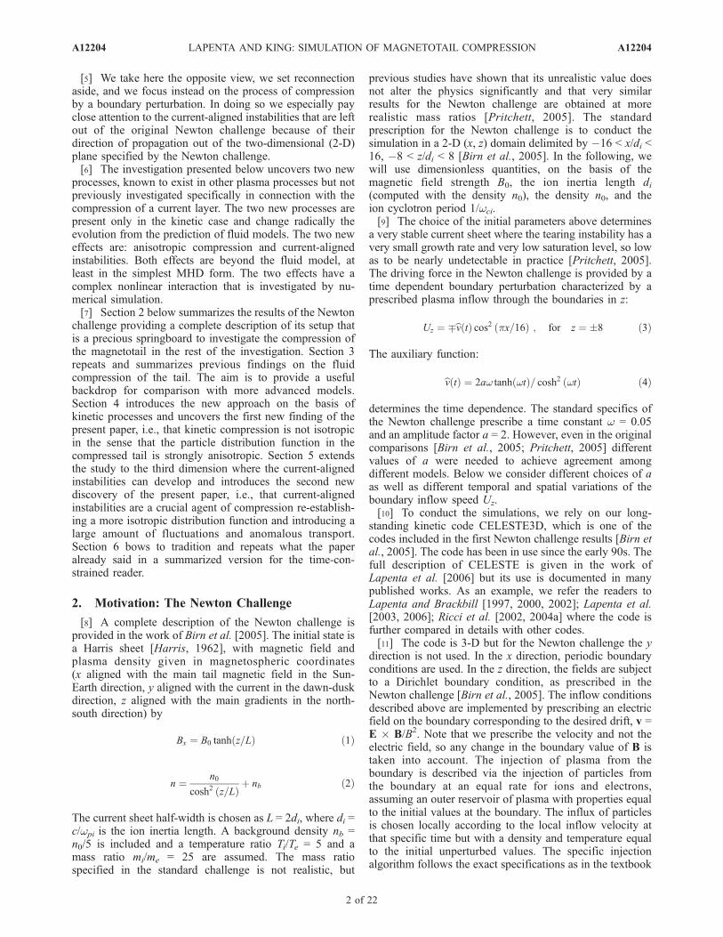
tion described above proceeds at very similar rates in allkinetic and Hall models reported by Birn et al. [2005], whenappropriate choices are made of the forcing parameters.However, the time of onset and the rate of reconnectionchange widely, depending very sensitively on the value theforcing amplitude a [Pritchett, 2005]. Furthermore, theNewton challenge gives different results for different codeimplementations (e.g., depending on the details of theboundary conditions) [Birn et al., 2005; Pritchett, 2005].Prompted by this evident but puzzling finding, we haveinvestigated the sensitivity of the results on the driving forceand on the accuracy of the calculation.[13] Figure 1 reports three paradigmatic results. Different

cases are shown with different boundary forcing and dif-ferent resolutions (but all with the same time step wpiDt =0.3). As the resolution is increased, the reconnection processprogresses more slowly and saturates at a lower amplitude.Conversely and trivially, as the forcing is increased, recon-nection progresses more swiftly and to a higher saturationrate. An additional effect on the saturation level is given bychanging the system size and allowing more islands togrow, affecting the saturation level [Karimabadi et al.,2005].[14] It is evident that the Newton challenge is very

sensitive to the accuracy of the calculation. Simulationswith different spatial resolutions or temporal resolutions ornumber of particles per cell lead to a different history of thereconnected flux. In particular, the reconnection developsearlier in the lower-resolution calculation.

Figure 1. Newton challenge. History of the reconnectedflux for three runs with different resolution and compressionamplitudes: 64 � 64 grid, with a = 3 (solid blue line); 32 �32 grid, with a = 3 (dashed red line); and 64 � 64 grid, witha = 1.5 (dotted black line). The reconnected magnetic flux iscomputed as the difference of the vector potential betweenthe x point and the o point. In 2-D simulations in the (x, z)plane this diagnostic is a direct measure of the reconnectedflux [Biskamp, 2005].

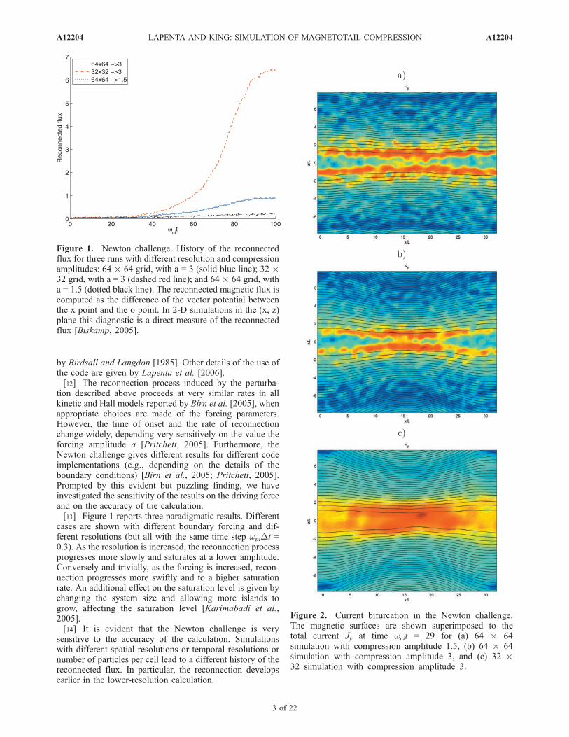
Figure 2. Current bifurcation in the Newton challenge.The magnetic surfaces are shown superimposed to thetotal current Jy at time wcit = 29 for (a) 64 � 64simulation with compression amplitude 1.5, (b) 64 � 64simulation with compression amplitude 3, and (c) 32 �32 simulation with compression amplitude 3.


3 of 22

A12204

[15] To investigate what allows reconnection in the low-resolution calculation to develop earlier, Figure 2 shows thecurrent and magnetic surfaces for three different simulationswith different drive and resolution at a stage of the simu-lation corresponding to the end of the boundary driving butbefore the reconnection develops. The magnetic surfacesintersect the (x, z) plane of the simulation along lines thatcan be easily computed as contour lines of the vectorpotential component Ay, shown in black in Figure 2.[16] The high-resolution calculations present a clear bi-

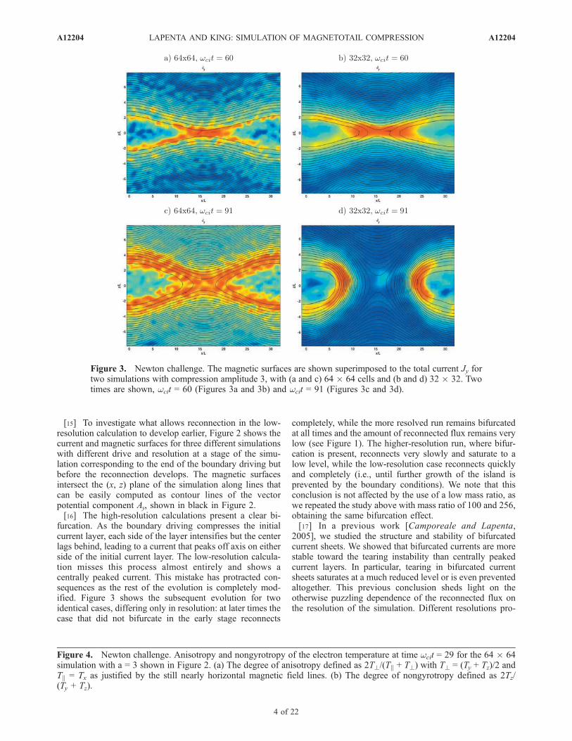
furcation. As the boundary driving compresses the initialcurrent layer, each side of the layer intensifies but the centerlags behind, leading to a current that peaks off axis on eitherside of the initial current layer. The low-resolution calcula-tion misses this process almost entirely and shows acentrally peaked current. This mistake has protracted con-sequences as the rest of the evolution is completely mod-ified. Figure 3 shows the subsequent evolution for twoidentical cases, differing only in resolution: at later times thecase that did not bifurcate in the early stage reconnects

completely, while the more resolved run remains bifurcatedat all times and the amount of reconnected flux remains verylow (see Figure 1). The higher-resolution run, where bifur-cation is present, reconnects very slowly and saturate to alow level, while the low-resolution case reconnects quicklyand completely (i.e., until further growth of the island isprevented by the boundary conditions). We note that thisconclusion is not affected by the use of a low mass ratio, aswe repeated the study above with mass ratio of 100 and 256,obtaining the same bifurcation effect.[17] In a previous work [Camporeale and Lapenta,

2005], we studied the structure and stability of bifurcatedcurrent sheets. We showed that bifurcated currents are morestable toward the tearing instability than centrally peakedcurrent layers. In particular, tearing in bifurcated currentsheets saturates at a much reduced level or is even preventedaltogether. This previous conclusion sheds light on theotherwise puzzling dependence of the reconnected flux onthe resolution of the simulation. Different resolutions pro-

Figure 3. Newton challenge. The magnetic surfaces are shown superimposed to the total current Jy fortwo simulations with compression amplitude 3, with (a and c) 64 � 64 cells and (b and d) 32 � 32. Twotimes are shown, wcit = 60 (Figures 3a and 3b) and wcit = 91 (Figures 3c and 3d).

Figure 4. Newton challenge. Anisotropy and nongyrotropy of the electron temperature at time wcit = 29 for the 64 � 64simulation with a = 3 shown in Figure 2. (a) The degree of anisotropy defined as 2T?/(Tk + T?) with T? = (Ty + Tz)/2 andTk = Tx as justified by the still nearly horizontal magnetic field lines. (b) The degree of nongyrotropy defined as 2Tz/(Ty + Tz).


4 of 22

A12204

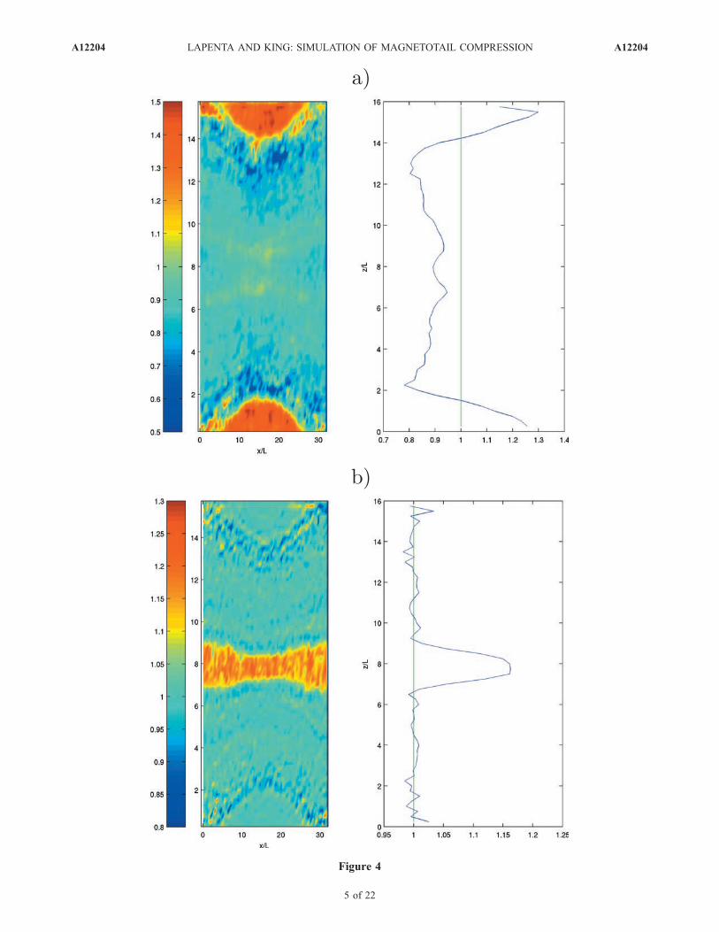
Figure 4


5 of 22

A12204

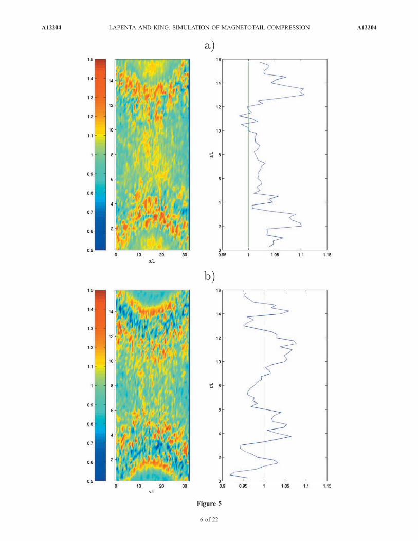
Figure 5


6 of 22

A12204

vide different levels of bifurcation which in turn providedifferent degrees of stability toward reconnection.[18] The bifurcation is caused by the presence of signif-

icant deviations from isotropy and gyrotropy [Camporealeand Lapenta, 2005]. Figure 4 shows the electron tempera-ture anisotropy and nongyrotropy at time wcit = 29 for thehigher resolution simulation shown in Figure 2. At thisstage, the compression phase is finished but the mainreconnection phase has not happened yet (see Figure 1).The electrons in the central layer are highly nongyrotropic.Furthermore, the parallel temperature exceeds the perpen-dicular temperature significantly within the layer and at itsedge, with the perpendicular component exceeding theparallel component only near the boundary, an effect ofthe compression wave caused by the boundary conditions(see below). The presence of T?/Tk < 1 within the layer is awell known cause of suppression of the tearing instability[Biskamp et al., 1970; Forslund, 1968; Pritchett, 2005].Figure 5 shows the ion temperature anisotropy andnongyrotropy at the same time for higher-resolutionsimulation shown in Figure 3. In between the two parts ofthe bifurcated current the ions remains isotropic andgyrotropic, the nongyrotropy and anisotropy remainsconfined in the off-center current peaks.[19] The electron nongyrotropy and anisotropy observed

in the Newton challenge may be removed in 3-D simula-tions by instabilities driven by temperature anisotropy anddeveloping in direction orthogonal or oblique to the (x, z) planeof the standard Newton challenge simulation [Karimabadiet al., 2004; Gary and Karimabadi, 2006]. However, asshown below other effects may act first to remove thebifurcation from even forming.[20] The phenomenological explanation provided above

fails to identify the root causes of the problem. Why is thecurrent bifurcating in the first place? That is, why anisotropyand nongyrotropy are created? Why is the compression notsimply leading to a centrally peaked current layer? The issueis crucial because even the lower-resolution calculation stillresolves the layer with sufficient accuracy to detect the typeof bifurcated layer observed in the higher-resolution calcu-lation. For example, the bifurcated current seen in Figure 2bwould still be resolved by approximately 10 cells in thelower-resolution case. So there must be some more subtleeffect missed by the lower-resolution calculations but that isnot just the trivial resolution of the layer itself. The rest of thepaper tries to resolve this issue.

3. Ideal MHD Model of Fluid Compression

[21] To study the effect of compression in a configurationtypical of the Earth magnetotail, we consider first thegeneral problem of compression of a plasma as modeledby MHD fluid equations. To investigate the issue we rely onthe ideal MHD code GrAALE (Grid Adaptation ArbitraryLagrangian Eulerian) [Lapenta, 2002].

[22] The GrAALE code is based on the ideal magneto-hydrodynamic (MHD) model. The equations governing theevolution of the plasma are [see, e.g., Goedbloed andPoedts, 2004]:

drdt

¼ �rr �~u ð5Þ

rd~u

dt¼ �r P þ B2

2m0

� �þ 1

m0

r �~B~B ð6Þ

rde

dt¼ �pr �~u ð7Þ

d

dt

~B

r

!¼~B

r� r~u ð8Þ

[23] The electric field is computed from Ohm’s law as,~E = �~u � ~B, and the current as, ~j = (r � ~B)/m0. Thepressure P is computed from the equation of state: P =er(g � 1) where g is the polytropic index, assumed hereto correspond to 5/3.[24] The equations above are solved using a Lagrangian

scheme [Bowers and Wilson, 1991; Lapenta, 2002]. In thepresent study, the grid is initially uniform, and is movedaccording to the local fluid velocity, resulting in a fullyLagrangian simulation. The time step is chosen as wciDt =7 � 10�5. To investigate the simplest type of compression,we consider first a 1-D compression of a stratified plasmawith properties varying along just the coordinate z, assum-ing uniformity along x and y.[25] A fundamental property of fluid models is that any

compression wave eventually leads to shocks [Zel’dovichand Raizer, 1968]. To verify the ability of the GrAALEcode to capture shocks correctly, we have considered anumber of Riemann problems in gas dynamics and MHDwhere the analytical solution is known [Lax, 1973].[26] As an example of a test problem, close to the types of

problems needed for the present study but still sufficientlysimple to have an analytical solution, we report here thecase of a uniform magnetized plasma with the magneticfield aligned with the z boundary (i.e., B is directed alongx). The compression is provided by a piston acting on eachboundary with constant speed. Perpendicular shocks aregenerated at each wall and propagate inward at a speed vsgiven by the Rankine-Hugoniot conditions [Gurnett andBhattacharjee, 2005]:

v2s ¼2d c2s1 þ d � g d � 1ð Þ=2ð Þv2A1� �

g � 1ð Þ dm � dð Þ ð9Þ

Figure 5. Newton challenge. Anisotropy and nongyrotropy of the ion temperature at time wcit = 29 for the 64 � 64simulation with a = 3 shown in Figure 2. (a) The degree of anisotropy defined as 2T?/(Tk + T?) with T? = (Ty + Tz)/2 andTk = Tx as justified by the still nearly horizontal magnetic field lines. (b) The degree of nongyrotropy defined as 2Tz/(Ty + Tz).


7 of 22

A12204

where the index 1 refers to the unshocked media notreached yet by the shock and the index 2 refers to theshocked media, cs1 (vA1) is the sound (Alfven) speed in theunshocked media. The shock strength is defined as d = r2/r1and the maximum strength is dm = (g + 1)/(g � 1) [Gurnettand Bhattacharjee, 2005].[27] The pistons are assumed to be turned on as a step

function at time t = 0. The two converging shocks arecreated and move at equal speed (see equation (9)) toconverge in the center where they reflect to return to thewalls where they reflect once more and converge againtoward the center in a repeating cycle. At each reflection theshocks travel in a plasma that is progressively more com-pressed, each time with a different Alfven and sound speed,and their speed changes. The changes in speed observed in

the simulations can be compared with the predictions fromtheory given by equation (9). The results of this comparisonare summarized in Table 1 where a remarkable agreement isfound.

4. Fluid Compression of Harris Current Sheets

[28] We apply the ideal MHD model described above tostudy the compression of the configuration prescribed bythe Newton challenge.[29] To initiate compression, a piston is assumed to

impart a step velocity increase on both walls of the plasmaat z = ±10. Between the zeroth and first time step the wallspeed goes from zero to 1/3 of the local magnetosonic speedat the plasma edge, where the sound speed is

cs =ffiffiffiffiffiffiffiffiffiffiffiffiffiffiffiffiffiffiffiffigðg � 1Þe

pand the magnetosonic speed is

vms =ffiffiffiffiffiffiffiffiffiffiffiffiffiffiffic2s þ v2A

p. These values are computed locally with

the edge magnetic field (B0) and density (nb).[30] The plasma is initially nonuniform with a uniform

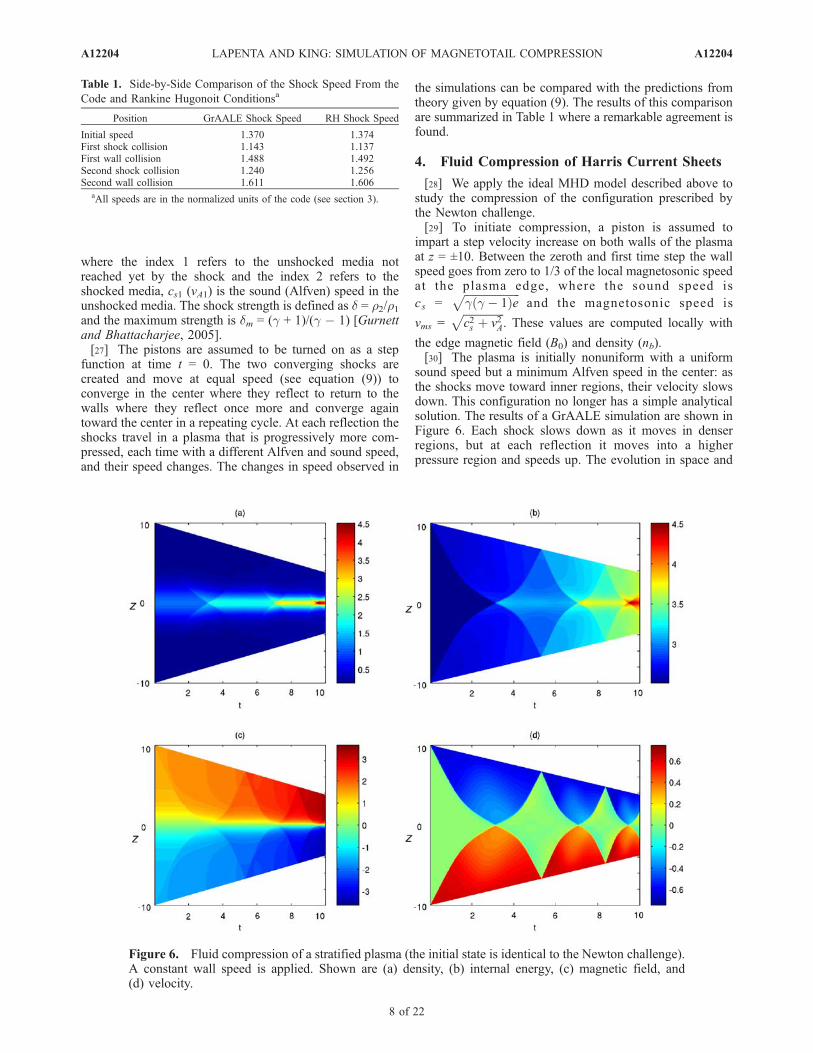
sound speed but a minimum Alfven speed in the center: asthe shocks move toward inner regions, their velocity slowsdown. This configuration no longer has a simple analyticalsolution. The results of a GrAALE simulation are shown inFigure 6. Each shock slows down as it moves in denserregions, but at each reflection it moves into a higherpressure region and speeds up. The evolution in space and

Figure 6. Fluid compression of a stratified plasma (the initial state is identical to the Newton challenge).A constant wall speed is applied. Shown are (a) density, (b) internal energy, (c) magnetic field, and(d) velocity.

Table 1. Side-by-Side Comparison of the Shock Speed From the

Code and Rankine Hugonoit Conditionsa

Position GrAALE Shock Speed RH Shock Speed

Initial speed 1.370 1.374First shock collision 1.143 1.137First wall collision 1.488 1.492Second shock collision 1.240 1.256Second wall collision 1.611 1.606

aAll speeds are in the normalized units of the code (see section 3).


8 of 22

A12204

time of a number of fluid quantities is shown in Figure 6where the horizontal axis is time and the vertical axis is theonly relevant spatial direction (z), the value of each quantityis reported in color. The presence of shocks is clearlymarked by the sharp jump in color in the space-time plot.The magnetic field is initially directed along the x direction,the action of perpendicular shocks alters its strength (seeFigure 6c) but leaves its direction unaltered.[31] Gentler discontinuities can be obtained if the piston

is activated more gently. We considered, besides the stepfunction case above (referred to as case 1 below), a linearramp-up (case 2) starting from zero and increasing linearlyso that at the end of the simulation the walls have moved bythe same total distance as in the previous case, and aquadratic ramp-up (case 3), also leading to the same totalcompression. As the law of motion of the piston is chosen topresent higher continuity at t = 0, going from a discontin-uous function (step function of Figure 6) to a function withdiscontinuous derivative (linear ramp up) and one withdiscontinuous second derivative (quadratic ramp up), thesolution presents gentler discontinuities.[32] The primary effect of the shocks (or of the other

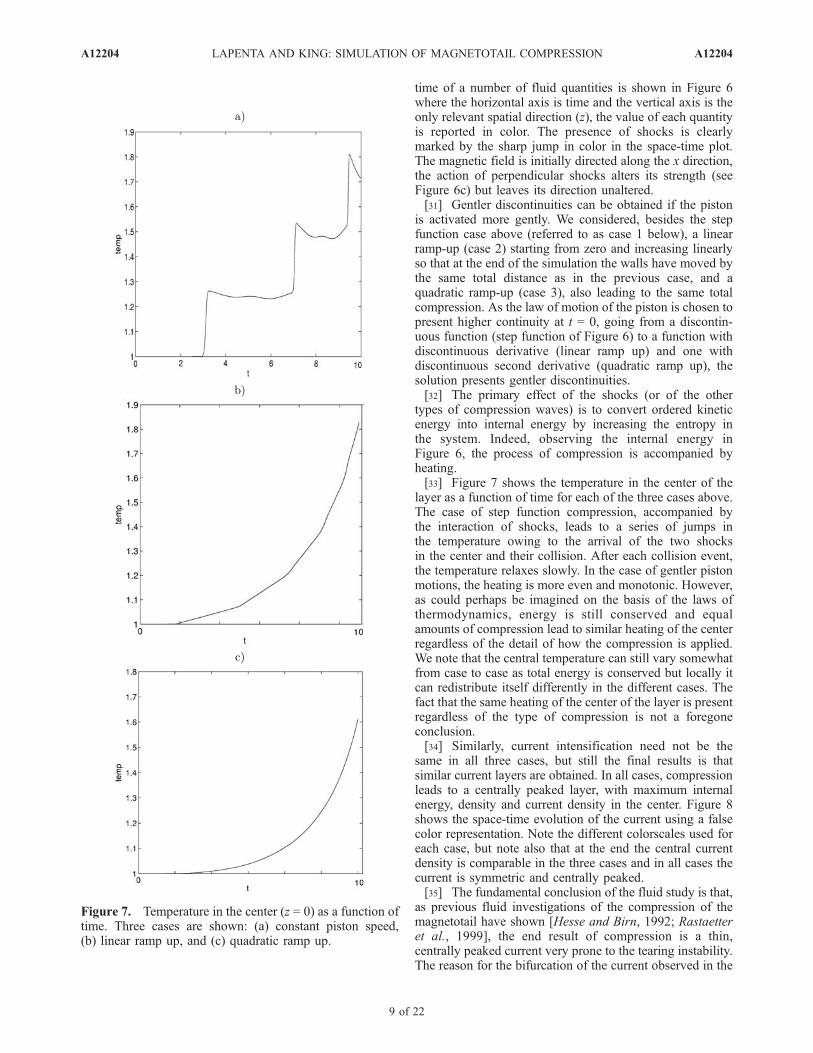
types of compression waves) is to convert ordered kineticenergy into internal energy by increasing the entropy inthe system. Indeed, observing the internal energy inFigure 6, the process of compression is accompanied byheating.[33] Figure 7 shows the temperature in the center of the

layer as a function of time for each of the three cases above.The case of step function compression, accompanied bythe interaction of shocks, leads to a series of jumps inthe temperature owing to the arrival of the two shocksin the center and their collision. After each collision event,the temperature relaxes slowly. In the case of gentler pistonmotions, the heating is more even and monotonic. However,as could perhaps be imagined on the basis of the laws ofthermodynamics, energy is still conserved and equalamounts of compression lead to similar heating of the centerregardless of the detail of how the compression is applied.We note that the central temperature can still vary somewhatfrom case to case as total energy is conserved but locally itcan redistribute itself differently in the different cases. Thefact that the same heating of the center of the layer is presentregardless of the type of compression is not a foregoneconclusion.[34] Similarly, current intensification need not be the

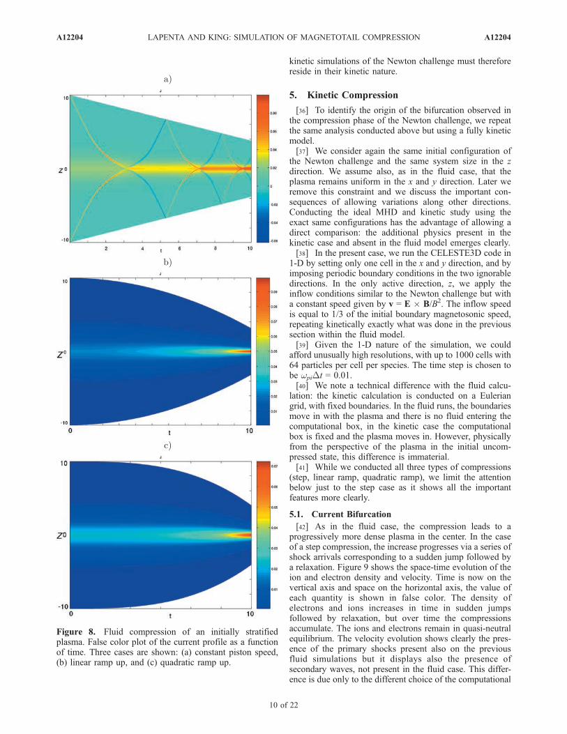
same in all three cases, but still the final results is thatsimilar current layers are obtained. In all cases, compressionleads to a centrally peaked layer, with maximum internalenergy, density and current density in the center. Figure 8shows the space-time evolution of the current using a falsecolor representation. Note the different colorscales used foreach case, but note also that at the end the central currentdensity is comparable in the three cases and in all cases thecurrent is symmetric and centrally peaked.[35] The fundamental conclusion of the fluid study is that,

as previous fluid investigations of the compression of themagnetotail have shown [Hesse and Birn, 1992; Rastaetteret al., 1999], the end result of compression is a thin,centrally peaked current very prone to the tearing instability.The reason for the bifurcation of the current observed in the

Figure 7. Temperature in the center (z = 0) as a function oftime. Three cases are shown: (a) constant piston speed,(b) linear ramp up, and (c) quadratic ramp up.


9 of 22

A12204

kinetic simulations of the Newton challenge must thereforereside in their kinetic nature.

5. Kinetic Compression

[36] To identify the origin of the bifurcation observed inthe compression phase of the Newton challenge, we repeatthe same analysis conducted above but using a fully kineticmodel.[37] We consider again the same initial configuration of

the Newton challenge and the same system size in the zdirection. We assume also, as in the fluid case, that theplasma remains uniform in the x and y direction. Later weremove this constraint and we discuss the important con-sequences of allowing variations along other directions.Conducting the ideal MHD and kinetic study using theexact same configurations has the advantage of allowing adirect comparison: the additional physics present in thekinetic case and absent in the fluid model emerges clearly.[38] In the present case, we run the CELESTE3D code in

1-D by setting only one cell in the x and y direction, and byimposing periodic boundary conditions in the two ignorabledirections. In the only active direction, z, we apply theinflow conditions similar to the Newton challenge but witha constant speed given by v = E � B/B2. The inflow speedis equal to 1/3 of the initial boundary magnetosonic speed,repeating kinetically exactly what was done in the previoussection within the fluid model.[39] Given the 1-D nature of the simulation, we could

afford unusually high resolutions, with up to 1000 cells with64 particles per cell per species. The time step is chosen tobe wpiDt = 0.01.[40] We note a technical difference with the fluid calcu-

lation: the kinetic calculation is conducted on a Euleriangrid, with fixed boundaries. In the fluid runs, the boundariesmove in with the plasma and there is no fluid entering thecomputational box, in the kinetic case the computationalbox is fixed and the plasma moves in. However, physicallyfrom the perspective of the plasma in the initial uncom-pressed state, this difference is immaterial.[41] While we conducted all three types of compressions

(step, linear ramp, quadratic ramp), we limit the attentionbelow just to the step case as it shows all the importantfeatures more clearly.

5.1. Current Bifurcation

[42] As in the fluid case, the compression leads to aprogressively more dense plasma in the center. In the caseof a step compression, the increase progresses via a series ofshock arrivals corresponding to a sudden jump followed bya relaxation. Figure 9 shows the space-time evolution of theion and electron density and velocity. Time is now on thevertical axis and space on the horizontal axis, the value ofeach quantity is shown in false color. The density ofelectrons and ions increases in time in sudden jumpsfollowed by relaxation, but over time the compressionsaccumulate. The ions and electrons remain in quasi-neutralequilibrium. The velocity evolution shows clearly the pres-ence of the primary shocks present also on the previousfluid simulations but it displays also the presence ofsecondary waves, not present in the fluid case. This differ-ence is due only to the different choice of the computational

Figure 8. Fluid compression of an initially stratifiedplasma. False color plot of the current profile as a functionof time. Three cases are shown: (a) constant piston speed,(b) linear ramp up, and (c) quadratic ramp up.


10 of 22

A12204

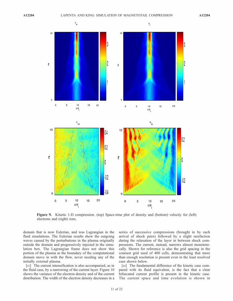
domain that is now Eulerian, and was Lagrangian in thefluid simulations. The Eulerian results show the outgoingwaves caused by the perturbations in the plasma originallyoutside the domain and progressively injected in the simu-lation box. The Lagrangian frame does not show thisportion of the plasma as the boundary of the computationaldomain move in with the flow, never needing any of theinitially external plasma.[43] The current intensification is also accompanied, as in

the fluid case, by a narrowing of the current layer. Figure 10shows the variance of the electron density and of the currentdistribution. The width of the electron density decreases in a

series of successive compressions (brought in by eacharrival of shock pairs) followed by a slight rarefactionduring the relaxation of the layer in between shock com-pressions. The current, instead, narrows almost monotoni-cally. Shown for reference is also the grid spacing in thecoarsest grid used of 400 cells, demonstrating that morethan enough resolution is present even in the least resolvedcase shown below.[44] The fundamental difference of the kinetic case com-

pared with its fluid equivalent, is the fact that a clearbifurcated current profile is present in the kinetic case.The current space and time evolution is shown in

Figure 9. Kinetic 1-D compression. (top) Space-time plot of density and (bottom) velocity for (left)electrons and (right) ions.


11 of 22

A12204

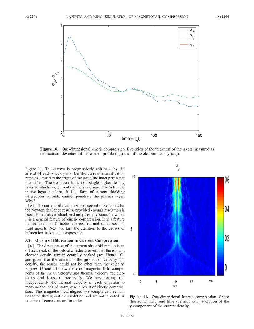
Figure 11. The current is progressively enhanced by thearrival of each shock pairs, but the current intensificationremains limited to the edges of the layer, the inner part is notintensified. The evolution leads to a single higher densitylayer in which two currents of the same sign remain limitedto the layer outskirts. It is a form of current shieldingwhereupon currents cannot penetrate the plasma layer.Why?[45] The current bifurcation was observed in Section 2 for

the Newton challenge results, provided enough resolution isused. The results of shock and ramp compressions show thatit is a general feature of kinetic compression. It is a featurethat is peculiar of kinetic compression and is not seen influid models. Next we turn the attention to the causes ofbifurcation in kinetic compression.

5.2. Origin of Bifurcation in Current Compression

[46] The direct cause of the current sheet bifurcation is anoff axis peak of the velocity. Indeed, given that the ion andelectron density remain centrally peaked (see Figure 10),and given that the current is the product of velocity anddensity, the reason could not be other than the velocity.Figures 12 and 13 show the cross magnetic field compo-nents of the mean velocity and thermal velocity for elec-trons and ions, respectively. We have computedindependently the thermal velocity in each direction tomeasure the lack of isotropy as a result of kinetic compres-sion. The magnetic field-aligned (x) components remainunaltered throughout the evolution and are not reported. Anumber of comments are in order.

Figure 10. One-dimensional kinetic compression. Evolution of the thickness of the layers measured asthe standard deviation of the current profile (sJy) and of the electron density (sre).

Figure 11. One-dimensional kinetic compression. Space(horizontal axis) and time (vertical axis) evolution of they component of the current density.


12 of 22

A12204

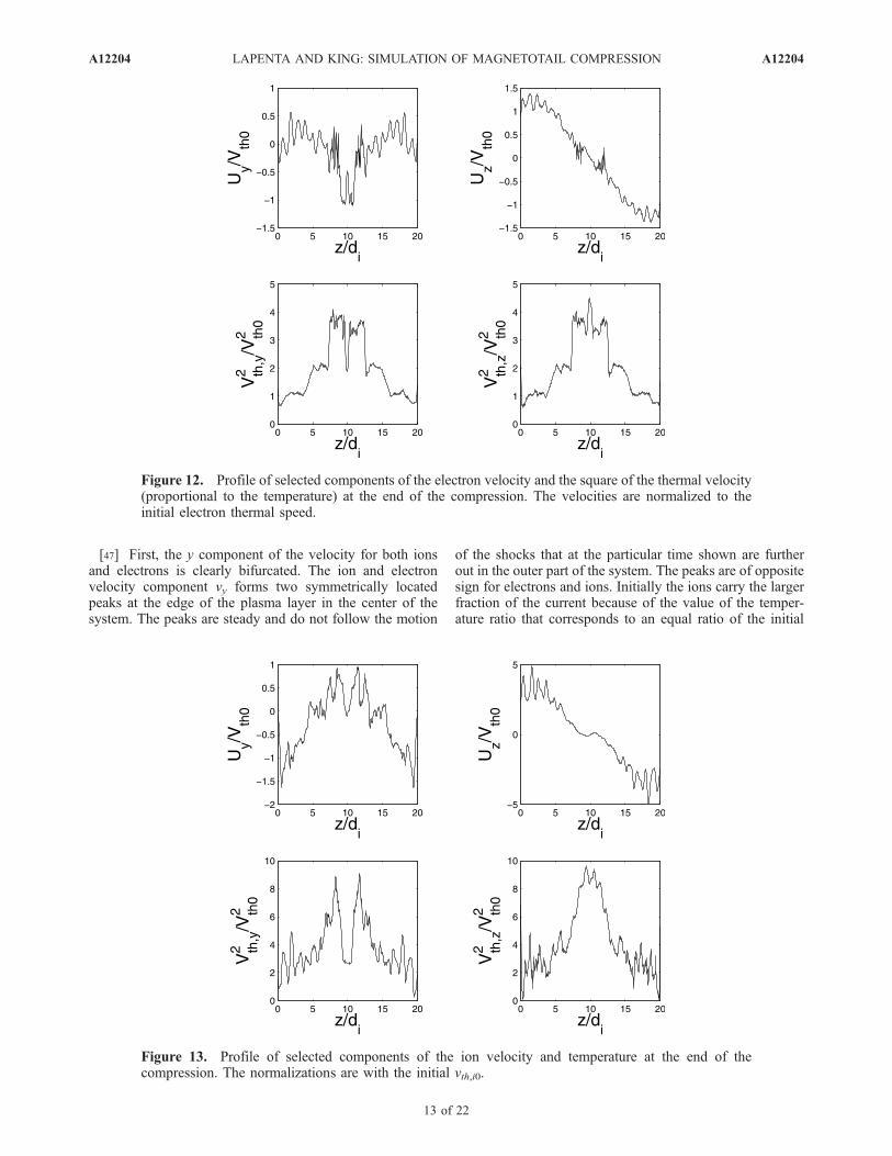
[47] First, the y component of the velocity for both ionsand electrons is clearly bifurcated. The ion and electronvelocity component vy forms two symmetrically locatedpeaks at the edge of the plasma layer in the center of thesystem. The peaks are steady and do not follow the motion

of the shocks that at the particular time shown are furtherout in the outer part of the system. The peaks are of oppositesign for electrons and ions. Initially the ions carry the largerfraction of the current because of the value of the temper-ature ratio that corresponds to an equal ratio of the initial

Figure 12. Profile of selected components of the electron velocity and the square of the thermal velocity(proportional to the temperature) at the end of the compression. The velocities are normalized to theinitial electron thermal speed.

Figure 13. Profile of selected components of the ion velocity and temperature at the end of thecompression. The normalizations are with the initial vth,i0.


13 of 22

A12204

currents for a Harris sheet. However, after shock compres-sion the electrons carry a great majority of the current. Thevelocities shown in Figures 12 and 13 are normalized totheir respective thermal velocity, in both cases they reach apeak value close to the respective initial thermal speed.Given that the initial ion thermal speed is smaller(about 0.447 times) than the electron thermal speed, the

electrons carry the larger part of the current aftercompression.[48] Second, except for the very center of the current

sheet, the plasma remains gyrotropic. The shocked plasmais highly anisotropic, as the heating is only in the cross fielddirection, while the field-aligned temperature remains unal-tered. However, it remains gyrotropic.

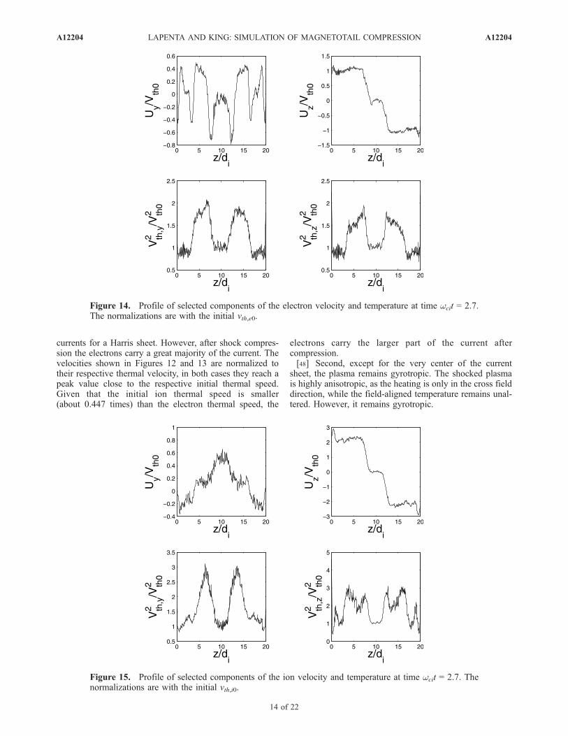
Figure 14. Profile of selected components of the electron velocity and temperature at time wcit = 2.7.The normalizations are with the initial vth,e0.

Figure 15. Profile of selected components of the ion velocity and temperature at time wcit = 2.7. Thenormalizations are with the initial vth,i0.


14 of 22

A12204

[49] This point is further analyzed in Figures 14 and 15that show the status of the average and thermal velocities attime wcit = 2.7, before the shocks first reach the center. Theshock is clearly identified in the plot of Uz where the leftmoving and right moving shocks are identified as thenarrow transition layers where the velocity drops from its

outer value to zero. The component Uy has an excursionfrom positive to negative at each shock location, an effect ofthe gyromotion that rotates the velocity of the particles inthe shock region from the z to the y direction. The plot ofthe component Uy is further complicated by the initial bellshape of its profile owing to the combination of Harris

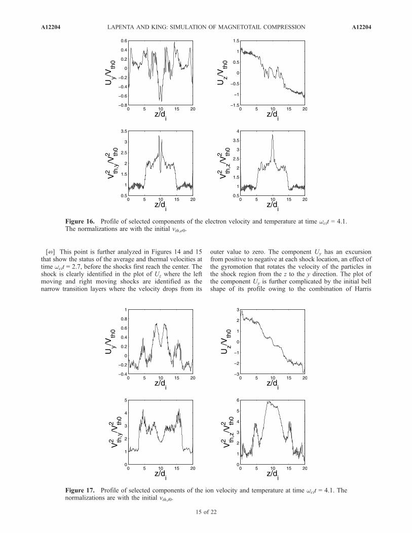
Figure 16. Profile of selected components of the electron velocity and temperature at time wcit = 4.1.The normalizations are with the initial vth,e0.

Figure 17. Profile of selected components of the ion velocity and temperature at time wcit = 4.1. Thenormalizations are with the initial vth,i0.


15 of 22

A12204

equilibrium and motionless background typical of theNewton (and GEM) challenge.[50] The thermal speeds show three distinct regions. The

innermost region is the plasma not yet reached by the shock,the next outer region is the plasma initially present in thesimulation box and already shocked. The outermost regionis the new fresh plasma injected at the boundary andrepresenting the infinite reservoir of plasma outside the

simulation box. In the shocked regions, the thermal speedhas been doubled by shock heating, in equal fractions inboth cross field directions, resulting in a completely gyro-tropic distribution. The regions outside the innermost part ofthe current layer are characterized by a strong magnetic fieldthat magnetizes both electrons and ions and keeps thedistribution gyrotropic.[51] In the outermost region of freshly injected plasma, a

number of secondary weak shocks can be identified in theslight discontinuities visible above the noise level in the Uz

components and much more clearly visible in the wideexcursion of the component Uy in the region of freshlyinjected plasma. The position of the excursions of Uy

correspond to the positions of the small jumps of thevelocity Uz indicative of weak secondary shocks.[52] The situation changes drastically after the shocks

reach the center, collide and reflect off each other. Figures 16and 17 shows the same four components of the thermal andaverage velocity for electrons and ions, respectively. Afterthe compression reaches the center, the central part does notretain its gyrotropy. The y component of the thermalvelocity is depleted with respect to the rest of the shockedplasma, while the z component is further enhanced. Corre-spondingly, the average velocity in the direction y forms abifurcated structure with a reduced speed in the center andtwo peaks off-center. The width of the depleted region islarger for the ions than for the electrons.[53] The reason for the lack of gyrotropy in the center is

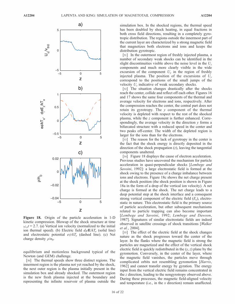
the fact that the shock energy is directly deposited in thedirection of the shock propagation (z), leaving the tangentialcomponents unaltered.[54] Figure 18 displays the cause of electron acceleration.

Previous studies have uncovered the mechanism for particleacceleration in quasi-perpendicular shocks [Lembege andSavoini, 1992]: a large electrostatic field is formed at theshock owing to the presence of a charge imbalance betweenions and electrons. Figure 18c shows the net charge presentat the shock position (the shock position is shown in Figure18a in the form of a drop of the vertical ion velocity). A netcharge is formed at the shock. The net charge leads to adeep potential step at the shock interface and a consequentstrong vertical component of the electric field (Ez), electro-static in nature. This electrostatic field is the primary sourceof particle acceleration, but other subsequent mechanismsrelated to particle trapping can also become important[Lembege and Savoini, 1992; Lembege and Dawson,1987]. Signatures of similar electrostatic fields are indeedobserved in satellite crossings of shock transitions [Walkeret al., 2004].[55] The effect of the electric field at the shock changes

nature as the shock progresses toward the center of thelayer. In the flanks where the magnetic field is strong theparticles are magnetized and the effect of the vertical shockelectric field is quickly redistributed in the (y, z) plane by thegyromotion. Conversely, in the center of the layer, wherethe magnetic field vanishes, the particles move throughcomplicated orbits not resembling gyromotion [Harris,1962] and cannot transfer energy by gyration. The energyinput from the vertical electric field remains concentrated inthe z direction, leading to the nongyrotropy observed above.During these processes, the magnetic field-aligned velocityand temperature (i.e., in the x direction) remain unaffected.

Figure 18. Origin of the particle acceleration in 1-Dkinetic compression. Blowup of the shock structure at timewcit = 2.7. (a) Vertical ion velocity (normalized to the initialion thermal speed). (b) Electric field dieE/kTe (solid line)and electrostatic potential ef/kTe (dashed line). (c) Netcharge density r/n0.


16 of 22

A12204

[56] The anisotropic and nongyrotropic nature of the ionand electron distribution function is further demonstrated bythe electron and ion pressure tensors (not shown). Thepresence of a sizable Pyz component demonstrate theimportance of nongyrotropy.[57] The existence of nongyrotropy and anisotropy is

itself the cause of the bifurcation of the average velocityand of the current [Sitnov et al., 2003]. A previous study ofbifurcated sheets [Camporeale and Lapenta, 2005] provid-ed a theory for the modeling of bifurcated currents. Bifur-cated currents are linked to the presence of significantdeviations from isotropy and gyrotropy. Based on the theoryof Schindler and Birn [2002] for general kinetic equilibriaof current sheets, Camporeale and Lapenta [2005] showedthat the presence of a nongyrotropic distribution function islinked to the existence of bifurcated equilibria. However,the analysis of stability described by Camporeale andLapenta [2005] also showed that such bifurcated equilibriatend to be unstable and decay rapidly to centrally peakedequilibria by the excitation and saturation of instabilities inthe lower-hybrid drift (LHD) range propagating along thecurrent direction y. The study conducted above owing to its1-D nature prevents any such instabilities from developing.The study typical of the Newton challenge, limited in the(x, z) plane also does not allow current-aligned instabilitiesin the LHD range to develop. In the next paragraph weconsider the effect of such instabilities by considering theirplane of evolution: (y, z).

6. Role of the Third Dimension

[58] In the preceding discussion we have focused on therole of processes developing in the (x, z) plane, the plane ofthe initial magnetic field and of the compression. In the fluidcase, nothing is added if the third dimension (y) is added.[59] In the kinetic case, in contrast, the third dimension is

crucial. Given the high cost of fully 3-D simulations thatresolve the systems at the small scales demonstrated by the1-D evolution shown above, we consider instead simula-tions on the (y, z) plane that complement the 2-D (x, z)

simulations and 1-D kinetic simulations shown above. Fully3-D effects could reserve more surprises as oblique modesare still neglected by the present analysis but have in somecircumstances been shown to play an important role[Lapenta and Brackbill, 2000; Ji et al., 2005]. Future workwill have to address this possibility.[60] In previous studies conducted in the (y, z) plane, two

types of instabilities have emerged to play an important rolein systems initially in a Harris equilibrium: electromagneticand electrostatic lower-hybrid drift (LHD) modes[Daughton, 2003] and kinking modes [Lapenta andBrackbill, 1997; Daughton, 1998]. While the two types ofmodes have been discovered in different periods and havegenerally different wavelengths, mathematically they are alldifferent eigensolutions of the same linearized problemdiffering only in the wavelength, but sharing a commonnature [Yoon et al., 2002]. The initial configuration ischaracterized by a background plasma superimposed to aHarris equilibrium and under these conditions the kinkingmodes assume the form of the so-called ion-ion kinkinstability [Daughton, 2002; Karimabadi et al., 2003]which is a form of Kelvin-Helmholtz instability (KHI)driven by the initial shear in velocity owing to the plasmabackground [Lapenta and Brackbill, 2002; Daughton,2002; Lapenta et al., 2003]. These instabilities, LHD andKHI, are indeed observed also in the present case.[61] Figure 19 shows the evolution in space and time of

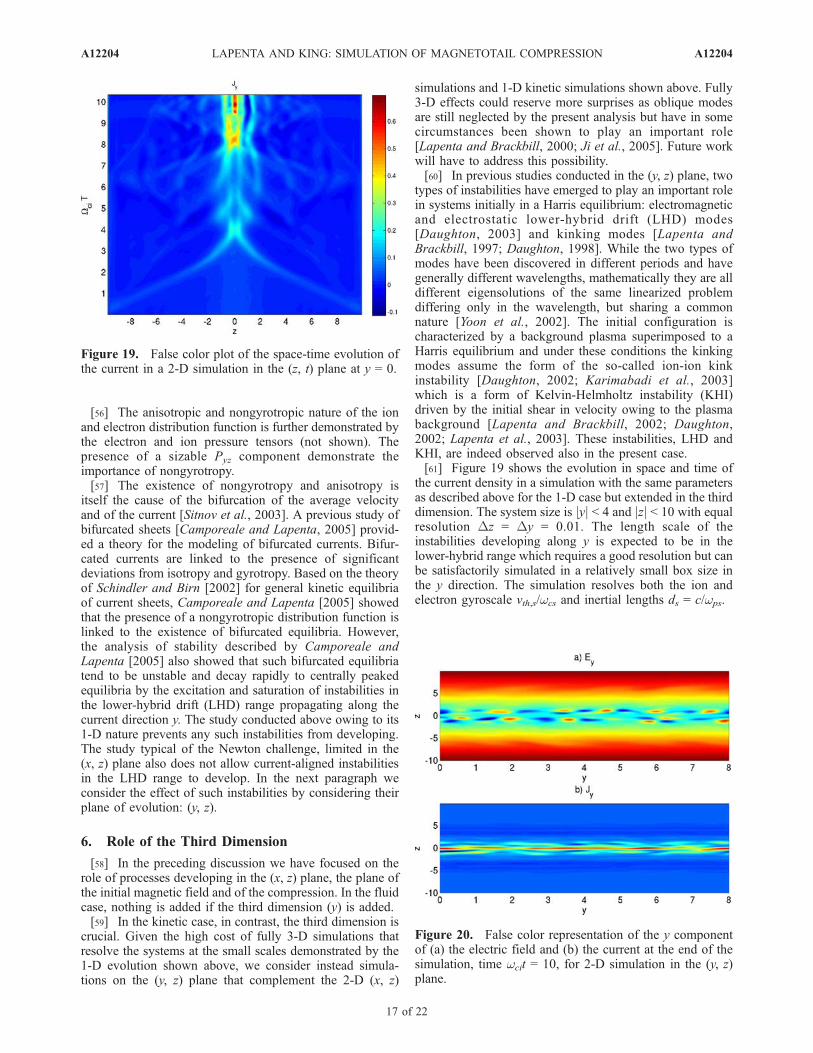
the current density in a simulation with the same parametersas described above for the 1-D case but extended in the thirddimension. The system size is jyj < 4 and jzj < 10 with equalresolution Dz = Dy = 0.01. The length scale of theinstabilities developing along y is expected to be in thelower-hybrid range which requires a good resolution but canbe satisfactorily simulated in a relatively small box size inthe y direction. The simulation resolves both the ion andelectron gyroscale vth,s/wcs and inertial lengths ds = c/wps.

Figure 19. False color plot of the space-time evolution ofthe current in a 2-D simulation in the (z, t) plane at y = 0.

Figure 20. False color representation of the y componentof (a) the electric field and (b) the current at the end of thesimulation, time wcit = 10, for 2-D simulation in the (y, z)plane.


17 of 22

A12204

[62] Figure 19 shows the specific space-time plane (x, t)at y = 0. As can be observed, the fundamental effect ofallowing instabilities to develop in the y direction is theessential removal of bifurcation and return of a centrallypeaked current sheet. Still side currents located off-centerbut not symmetrically are present.[63] The structure of the final current sheet is investigated

further in Figure 20 that shows the structure of they component of the current and of the electric field at theend of the run. The current is no longer straight and acquiresa wavy structure. Previous work [Lapenta and Brackbill,2002; Daughton, 2002] has investigated the nature of suchcurrent sheet kink in the magnetotail. A thick current sheetis unstable to modes developing in the lower-hybrid range,including both purely electrostatic and electromagneticmodes [Daughton, 2003]. The latter are directly responsiblefor kinking the current [Lapenta and Brackbill, 1997;Daughton, 2003] while the former act indirectly to kinkthe current sheet by inducing a Kelvin-Helmholtz instability[Lapenta and Brackbill, 2002; Daughton, 2002; Lapenta etal., 2003]. Note that in the present study the LHD rangemodes develop in an anisotropic system where besides thepure lower-hybrid drift instability also other modes arepresent [Gary and Karimabadi, 2006] with wavelengthscomparable to those seen in the electromagnetic branch ofthe LHD, making the precise nature of the observed wavespectrum mixed.[64] The results above are relative to a very low mass

ratio, and modes developing in the (y, z) plane are known to

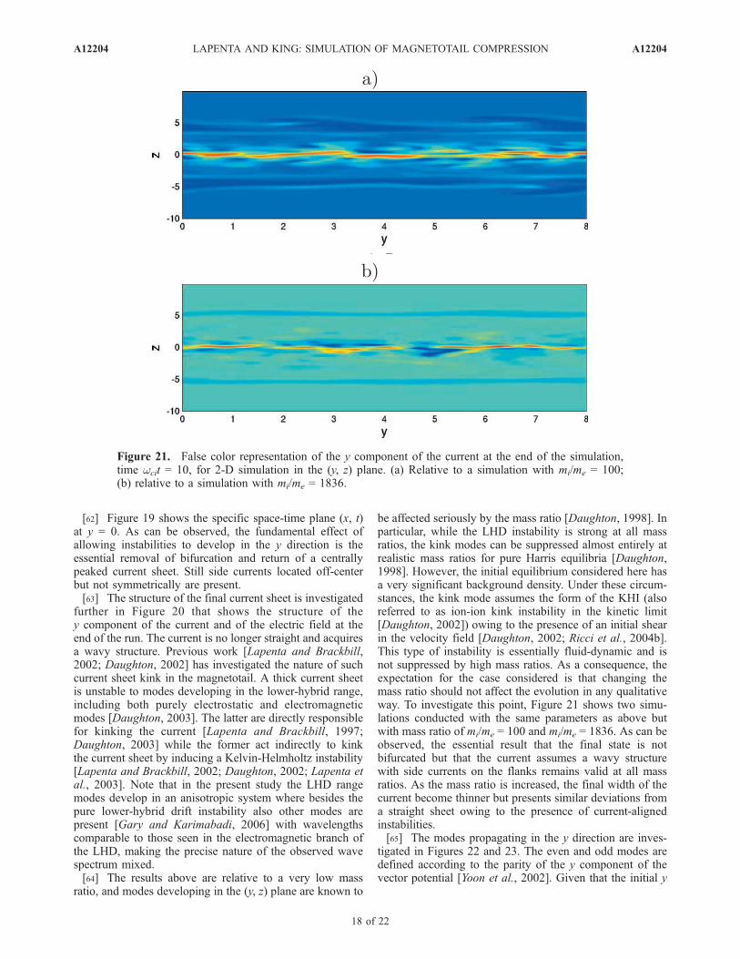
be affected seriously by the mass ratio [Daughton, 1998]. Inparticular, while the LHD instability is strong at all massratios, the kink modes can be suppressed almost entirely atrealistic mass ratios for pure Harris equilibria [Daughton,1998]. However, the initial equilibrium considered here hasa very significant background density. Under these circum-stances, the kink mode assumes the form of the KHI (alsoreferred to as ion-ion kink instability in the kinetic limit[Daughton, 2002]) owing to the presence of an initial shearin the velocity field [Daughton, 2002; Ricci et al., 2004b].This type of instability is essentially fluid-dynamic and isnot suppressed by high mass ratios. As a consequence, theexpectation for the case considered is that changing themass ratio should not affect the evolution in any qualitativeway. To investigate this point, Figure 21 shows two simu-lations conducted with the same parameters as above butwith mass ratio of mi/me = 100 and mi/me = 1836. As can beobserved, the essential result that the final state is notbifurcated but that the current assumes a wavy structurewith side currents on the flanks remains valid at all massratios. As the mass ratio is increased, the final width of thecurrent become thinner but presents similar deviations froma straight sheet owing to the presence of current-alignedinstabilities.[65] The modes propagating in the y direction are inves-

tigated in Figures 22 and 23. The even and odd modes aredefined according to the parity of the y component of thevector potential [Yoon et al., 2002]. Given that the initial y

Figure 21. False color representation of the y component of the current at the end of the simulation,time wcit = 10, for 2-D simulation in the (y, z) plane. (a) Relative to a simulation with mi/me = 100;(b) relative to a simulation with mi/me = 1836.


18 of 22

A12204

component of the vector potential in a Harris equilibrium iseven:

Ay z; t ¼ 0ð Þ ¼ �B0L log coshz

Lð10Þ

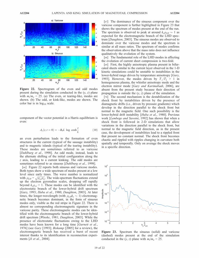
an even perturbation leads to the formation of evenstructures in the current (typical of the sausage instability)and to magnetic islands (typical of the tearing instability).These modes are sometimes referred to as varicose[Dahlburg et al., 1998]. An odd mode, instead, leads tothe alternate shifting of the initial configuration along thez axis, leading to a current kinking. The odd modes aresometimes referred to as sinuous [Dahlburg et al., 1998].[66] Figure 22 reports both sinuous and varicose modes.

Both types show a wide spectrum of modes present at a lowlevel since early times. The wave number is normalizedwith rLH =

ffiffiffiffiffiffiffiffiffiffiffircerci

p. The wide-spectrum fluctuations extend

up the electron gyroradius scales, dropping off rapidlybeyond kyrce > 1. These modes can be identified with theelectrostatic branch of the lower-hybrid drift spectrum[Gary, 1993; Huba et al., 1980; Daughton, 2003]. At latertimes, the longer-wavelength (with rLHky � 1) electromag-netic branch becomes dominant, in the form of sinuousmodes only, visible as the red stripe in Figure 22. There isalmost no corresponding electromagnetic signature in thevaricose parity. These electromagnetic modes can be iden-tified with the electromagnetic branch of the lower-hybriddrift spectrum [Winske, 1981; Daughton, 2003]. While thepresence of electrostatic fluctuations owing to the LHDmodes have been known for a long time [Gurnett et al.,1976] (see Gary [1993]; Biskamp [2005] for a review), theelectromagnetic branch has received a burst of recentinterest thanks to its identification in reconnection experi-ments [Ji et al., 2004].

[67] The dominance of the sinuous component over thevaricose component is further highlighted in Figure 23 thatshows the spectrum of modes present at the end of the run.The spectrum is observed to peak at around kyrLH � 1 asexpected for the electromagnetic branch of the LHD spec-trum [Daughton, 2003]. The sinuous modes are observed todominate over the varicose modes and the spectrum issimilar at all mass ratios. The spectrum of modes confirmsthe observation above that the mass ratio does not influencequalitatively the evolution of the system.[68] The fundamental role of the LHD modes in affecting

the evolution of current sheet compression is two-fold.[69] First, the highly anisotropic plasma present in bifur-

cated sheets similar to the current layer observed in the 1-Dkinetic simulations could be unstable to instabilities in thelower-hybrid range driven by temperature anisotropy [Gary,1993]. However, the modes driven by T?/Tk > 1 inhomogeneous plasma, the whistler anisotropy mode and theelectron mirror mode [Gary and Karimabadi, 2006], areabsent from the present study because their direction ofpropagation is outside the (y, z) plane of the simulation.[70] The second mechanism is the destabilization of the

shock front by instabilities driven by the presence ofdiamagnetic drifts (i.e., driven by pressure gradients) whichdevelop in the direction parallel to the shock front butnormal to the magnetic field. One such possibility is thelower-hybrid drift instability [Huba et al., 1980]. Previouswork [Lembege and Savoini, 1992] has shown that when ashock front is followed in 2-D simulations that allowvariations in the direction parallel to the shock front, butnormal to the magnetic field direction, as in the presentcase, the development of instabilities lead to a rippled frontthat present no constant normal. The shock front becomeschaotic and rippled with ripples changing in curvature bothspatially and temporally. Only on average the shock movesin a specific direction.

Figure 22. Spectrogram of the even and odd modespresent during the simulation conducted in the (y, z) planewith mi/me = 25. (a) The even, or tearing-like, modes areshown. (b) The odd, or kink-like, modes are shown. Thecolor bar is in log10 scale.

Figure 23. Spectrum the sinuous (solid) and varicose(dashed) modes present at the end of the simulationconducted in the (y, z) plane with mi/me = 25.


19 of 22

A12204

[71] In contrast, 2-D shock calculations conducted in theplane of the shock direction and of the magnetic field (i.e.,the (x, z) plane) show no such effect. The pressure gradientdriven instabilities are not captured because their directionof propagation is normal to the plane of the simulation andthe magnetic field imposes a constraint on the shock surfaceand prevents its rippling. We note that the laminarity of thecompression front in the (x, z) plane is indeed observed inFigures 2 and 3.[72] The possibility for the presence of the type of action

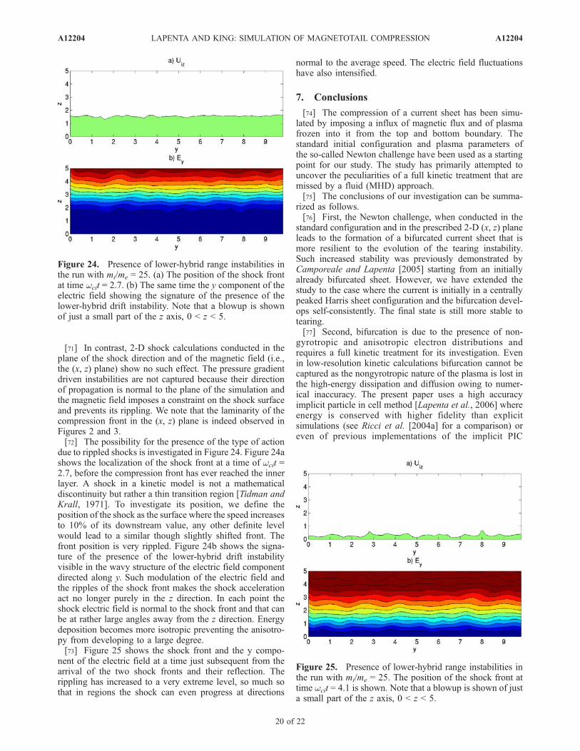
due to rippled shocks is investigated in Figure 24. Figure 24ashows the localization of the shock front at a time of wcit =2.7, before the compression front has ever reached the innerlayer. A shock in a kinetic model is not a mathematicaldiscontinuity but rather a thin transition region [Tidman andKrall, 1971]. To investigate its position, we define theposition of the shock as the surface where the speed increasesto 10% of its downstream value, any other definite levelwould lead to a similar though slightly shifted front. Thefront position is very rippled. Figure 24b shows the signa-ture of the presence of the lower-hybrid drift instabilityvisible in the wavy structure of the electric field componentdirected along y. Such modulation of the electric field andthe ripples of the shock front makes the shock accelerationact no longer purely in the z direction. In each point theshock electric field is normal to the shock front and that canbe at rather large angles away from the z direction. Energydeposition becomes more isotropic preventing the anisotro-py from developing to a large degree.[73] Figure 25 shows the shock front and the y compo-

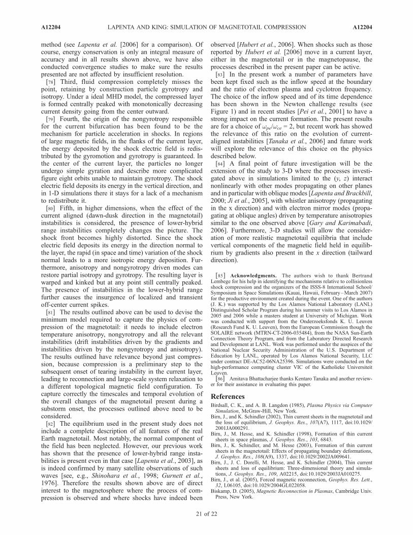
nent of the electric field at a time just subsequent from thearrival of the two shock fronts and their reflection. Therippling has increased to a very extreme level, so much sothat in regions the shock can even progress at directions

normal to the average speed. The electric field fluctuationshave also intensified.

7. Conclusions

[74] The compression of a current sheet has been simu-lated by imposing a influx of magnetic flux and of plasmafrozen into it from the top and bottom boundary. Thestandard initial configuration and plasma parameters ofthe so-called Newton challenge have been used as a startingpoint for our study. The study has primarily attempted touncover the peculiarities of a full kinetic treatment that aremissed by a fluid (MHD) approach.[75] The conclusions of our investigation can be summa-

rized as follows.[76] First, the Newton challenge, when conducted in the

standard configuration and in the prescribed 2-D (x, z) planeleads to the formation of a bifurcated current sheet that ismore resilient to the evolution of the tearing instability.Such increased stability was previously demonstrated byCamporeale and Lapenta [2005] starting from an initiallyalready bifurcated sheet. However, we have extended thestudy to the case where the current is initially in a centrallypeaked Harris sheet configuration and the bifurcation devel-ops self-consistently. The final state is still more stable totearing.[77] Second, bifurcation is due to the presence of non-

gyrotropic and anisotropic electron distributions andrequires a full kinetic treatment for its investigation. Evenin low-resolution kinetic calculations bifurcation cannot becaptured as the nongyrotropic nature of the plasma is lost inthe high-energy dissipation and diffusion owing to numer-ical inaccuracy. The present paper uses a high accuracyimplicit particle in cell method [Lapenta et al., 2006] whereenergy is conserved with higher fidelity than explicitsimulations (see Ricci et al. [2004a] for a comparison) oreven of previous implementations of the implicit PIC

Figure 24. Presence of lower-hybrid range instabilities inthe run with mi/me = 25. (a) The position of the shock frontat time wcit = 2.7. (b) The same time the y component of theelectric field showing the signature of the presence of thelower-hybrid drift instability. Note that a blowup is shownof just a small part of the z axis, 0 < z < 5.

Figure 25. Presence of lower-hybrid range instabilities inthe run with mi/me = 25. The position of the shock front attime wcit = 4.1 is shown. Note that a blowup is shown of justa small part of the z axis, 0 < z < 5.


20 of 22

A12204

method (see Lapenta et al. [2006] for a comparison). Ofcourse, energy conservation is only an integral measure ofaccuracy and in all results shown above, we have alsoconducted convergence studies to make sure the resultspresented are not affected by insufficient resolution.[78] Third, fluid compression completely misses the

point, retaining by construction particle gyrotropy andisotropy. Under a ideal MHD model, the compressed layeris formed centrally peaked with monotonically decreasingcurrent density going from the center outward.[79] Fourth, the origin of the nongyrotropy responsible

for the current bifurcation has been found to be themechanism for particle acceleration in shocks. In regionsof large magnetic fields, in the flanks of the current layer,the energy deposited by the shock electric field is redis-tributed by the gyromotion and gyrotropy is guaranteed. Inthe center of the current layer, the particles no longerundergo simple gyration and describe more complicatedfigure eight orbits unable to maintain gyrotropy. The shockelectric field deposits its energy in the vertical direction, andin 1-D simulations there it stays for a lack of a mechanismto redistribute it.[80] Fifth, in higher dimensions, when the effect of the

current aligned (dawn-dusk direction in the magnetotail)instabilities is considered, the presence of lower-hybridrange instabilities completely changes the picture. Theshock front becomes highly distorted. Since the shockelectric field deposits its energy in the direction normal tothe layer, the rapid (in space and time) variation of the shocknormal leads to a more isotropic energy deposition. Fur-thermore, anisotropy and nongyrotropy driven modes canrestore partial isotropy and gyrotropy. The resulting layer iswarped and kinked but at any point still centrally peaked.The presence of instabilities in the lower-hybrid rangefurther causes the insurgence of localized and transientoff-center current spikes.[81] The results outlined above can be used to devise the

minimum model required to capture the physics of com-pression of the magnetotail: it needs to include electrontemperature anisotropy, nongyrotropy and all the relevantinstabilities (drift instabilities driven by the gradients andinstabilities driven by the nongyrotropy and anisotropy).The results outlined have relevance beyond just compres-sion, because compression is a preliminary step to thesubsequent onset of tearing instability in the current layer,leading to reconnection and large-scale system relaxation toa different topological magnetic field configuration. Tocapture correctly the timescales and temporal evolution ofthe overall changes of the magnetotail present during asubstorm onset, the processes outlined above need to beconsidered.[82] The equilibrium used in the present study does not

include a complete description of all features of the realEarth magnetotail. Most notably, the normal component ofthe field has been neglected. However, our previous workhas shown that the presence of lower-hybrid range insta-bilities is present even in that case [Lapenta et al., 2003], asis indeed confirmed by many satellite observations of suchwaves [see, e.g., Shinohara et al., 1998; Gurnett et al.,1976]. Therefore the results shown above are of directinterest to the magnetosphere where the process of com-pression is observed and where shocks have indeed been

observed [Hubert et al., 2006]. When shocks such as thosereported by Hubert et al. [2006] move in a current layer,either in the magnetotail or in the magnetopause, theprocesses described in the present paper can be active.[83] In the present work a number of parameters have

been kept fixed such as the inflow speed at the boundaryand the ratio of electron plasma and cyclotron frequency.The choice of the inflow speed and of its time dependencehas been shown in the Newton challenge results (seeFigure 1) and in recent studies [Pei et al., 2001] to have astrong impact on the current formation. The present resultsare for a choice of wpe/wce = 2, but recent work has showedthe relevance of this ratio on the evolution of current-aligned instabilities [Tanaka et al., 2006] and future workwill explore the relevance of this choice on the physicsdescribed below.[84] A final point of future investigation will be the

extension of the study to 3-D where the processes investi-gated above in simulations limited to the (y, z) interactnonlinearly with other modes propagating on other planesand in particular with oblique modes [Lapenta and Brackbill,2000; Ji et al., 2005], with whistler anisotropy (propagatingin the x direction) and with electron mirror modes (propa-gating at oblique angles) driven by temperature anisotropiessimilar to the one observed above [Gary and Karimabadi,2006]. Furthermore, 3-D studies will allow the consider-ation of more realistic magnetotail equilibria that includevertical components of the magnetic field held in equilib-rium by gradients also present in the x direction (tailwarddirection).

[85] Acknowledgments. The authors wish to thank BertrandLembege for his help in identifying the mechanisms relative to collisionlessshock compression and the organizers of the ISSS-8 International School/Symposium in Space Simulations (Kauai, Hawaii, February–March 2007)for the productive environment created during the event. One of the authors(J. K.) was supported by the Los Alamos National Laboratory (LANL)Distinguished Scholar Program during his summer visits to Los Alamos in2005 and 2006 while a masters student at University of Michigan. Workwas conducted with support from the Onderzoeksfonds K. U. Leuven(Research Fund K. U. Leuven), from the European Commission though theSOLAIRE network (MTRN-CT-2006-035484), from the NASA Sun-EarthConnection Theory Program, and from the Laboratory Directed Researchand Development at LANL. Work was performed under the auspices of theNational Nuclear Security Administration of the U.S. Department ofEducation by LANL, operated by Los Alamos National Security, LLCunder contract DE-AC52-06NA25396. Simulations were conducted on thehigh-performance computing cluster VIC of the Katholieke UniversiteitLeuven.[86] Amitava Bhattacharjee thanks Kentaro Tanaka and another review-

er for their assistance in evaluating this paper.

ReferencesBirdsall, C. K., and A. B. Langdon (1985), Plasma Physics via ComputerSimulation, McGraw-Hill, New York.

Birn, J., and K. Schindler (2002), Thin current sheets in the magnetotail andthe loss of equilibrium, J. Geophys. Res., 107(A7), 1117, doi:10.1029/2001JA000291.

Birn, J., M. Hesse, and K. Schindler (1998), Formation of thin currentsheets in space plasmas, J. Geophys. Res., 103, 6843.

Birn, J., K. Schindler, and M. Hesse (2003), Formation of thin currentsheets in the magnetotail: Effects of propagating boundary deformations,J. Geophys. Res., 108(A9), 1337, doi:10.1029/2002JA009641.

Birn, J., J. C. Dorelli, M. Hesse, and K. Schindler (2004), Thin currentsheets and loss of equilibrium: Three-dimensional theory and simula-tions, J. Geophys. Res., 109, A02215, doi:10.1029/2003JA010275.

Birn, J., et al. (2005), Forced magnetic reconnection, Geophys. Res. Lett.,32, L06105, doi:10.1029/2004GL022058.

Biskamp, D. (2005), Magnetic Reconnection in Plasmas, Cambridge Univ.Press, New York.


21 of 22

A12204

Biskamp, D., R. Sagdeev, and K. Schindler (1970), Nonlinear evolution ofthe tearing instability in the geomagnetic tail, Cosmic Electrodyn., 1, 297.

Bowers, R., and J. Wilson (1991), Numerical Modeling in Applied Physics,Jones & Bartlett Publ., Sudbury, Mass.

Camporeale, E., and G. Lapenta (2005), Model of bifurcated current sheetsin the Earth’s magnetotail: Equilibrium and stability, J. Geophys. Res.,110, A07206, doi:10.1029/2004JA010779.

Dahlburg, R. B., P. Boncinelli, and G. Einaudi (1998), The evolution of aplane jet in a neutral sheet, Phys. Plasmas, 5, 79.

Daughton, W. (1998), Kinetic theory of the drift kink instability in a currentsheet, J. Geophys. Res., 103, 29,429.

Daughton, W. (2002), Nonlinear dynamics of thin current sheets, Phys.Plasmas, 9, 3668.

Daughton, W. (2003), Electromagnetic properties of the lower-hybrid driftinstability in a thin current sheet, Phys. Plasmas, 10, 3103.

Forslund, D. (1968), A model of the plasma sheet in the Earth’s magneto-sphere, Ph.D thesis, Princeton Univ., Princeton, N. J.

Gary, S. (1993), Theory of Space Plasma Microinstabilities, CambridgeUniv. Press, New York.

Gary, S., and H. Karimabadi (2006), Linear theory of electron temperatureanisotropy instabilities: Whistler, mirror, and Weibel, J. Geophys. Res.,111, A11224, doi:10.1029/2006JA011764.

Goedbloed, H., and S. Poedts (2004), Principles of Magnetohydrody-namics, Cambridge Univ. Press, New York.

Gurnett, D. A., and A. Bhattacharjee (2005), Introduction to Plasma Phy-sics: With Space and Laboratory Applications, Cambridge Univ. Press,New York.

Gurnett, D. A., L. A. Frank, and R. P. Lepping (1976), Plasma waves in thedistant magnetotail, J. Geophys. Res., 81, 6059.

Harris, E. (1962), On a plasma sheath separating regions of oppositelydirected magnetic field, Nuovo Cimento, 23, 115.

Hesse, M., and J. Birn (1992), Three-dimensional MHD modeling of mag-netotail dynamics for different polytropic indices, J. Geophys. Res., 97,3965.

Hesse, M., D. Winske, and J. Birn (1996), Hybrid modelling of the forma-tion of thin current sheets in the magnetotail, Eur. Space Agency, Spec.Publ., 389, 231.

Huba, J. D., J. F. Drake, and N. T. Gladd (1980), Lower-hybrid-drift in-stability in field reversed plasmas, Phys. Fluids, 23, 552.

Hubert, B., M. Palmroth, T. V. Laitinen, P. Janhunen, S. E. Milan, A. Grocott,S. W. H. Cowley, T. Pulkkinen, and J.-C. Gerard (2006), Compression ofthe Earth’s magnetotail by interplanetary shocks directly drives transientmagnetic flux closure, Geophys. Res. Lett., 33, L10105, doi:10.1029/2006GL026008.

Ishizawa, A., R. Horiuchi, and H. Ohtani (2004), Two-scale structure of thecurrent layer controlled by meandering motion during steady-state colli-sionless driven reconnection, Phys. Plasmas, 11, 3579.

Ji, H., S. Terry, M. Yamada, R. Kulsrud, A. Kuritsyn, and Y. Ren (2004),Electromagnetic fluctuations during fast reconnection in a laboratoryplasma, Phys. Rev. Lett., 92, 115,001.

Ji, H., R. Kulsrud, W. Fox, and M. Yamada (2005), An obliquely propagat-ing electromagnetic drift instability in the lower hybrid frequency range,J. Geophys. Res., 110, A08212, doi:10.1029/2005JA011188.

Kallenrode, M.-B. (2004), Space Physics: An Introduction to Plasmas andParticles in the Heliosphere and Magnetospheres, Springer, New York.

Karimabadi, H., W. Daughton, P. L. Pritchett, and D. Krauss-Varban (2003),Ion-ion kink instability in the magnetotail: 1. Linear theory, J. Geophys.Res., 108(A11), 1400, doi:10.1029/2003JA010026.

Karimabadi, H., W. Daughton, and K. B. Quest (2004), Role of electrontemperature anisotropy in the onset of magnetic reconnection, Geophys.Res. Lett., 31, L18801, doi:10.1029/2004GL020791.

Karimabadi, H., W. Daughton, and K. B. Quest (2005), Physics of satura-tion of collisionless tearing mode as a function of guide field, J. Geophys.Res., 110, A03214, doi:10.1029/2004JA010749.

Karpen, J. T., S. K. Antiochos, and C. R. Devore (1990), On the formationof current sheets in the solar corona, Astrophys. J., 356, L67.

Krauss-Varban, D., and N. Omidi (1995), Large-scale hybrid simulations ofthe magnetotail during reconnection, Geophys. Res. Lett., 22, 3271.

Lapenta, G. (2002), Grid adaptation and remapping for Arbitrary Lagran-gian Eulerian (ALE) methods paper presented at 8th International Con-ference on Numerical Grid Generation in Computational FieldSimulations, Int. Soc. of Grid Gener., Honolulu, Hawaii, 2–6 June.

Lapenta, G., and J. Brackbill (1997), A kinetic theory for the drift-kinkinstability, J. Geophys. Res., 102, 27,099.

Lapenta, G., and J. Brackbill (2000), 3D reconnection due to obliquemodes: A simulation of harris current sheets, Nonlinear Processes Geo-phys., 7, 151.

Lapenta, G., and J. Brackbill (2002), Nonlinear evolution of the lowerhybrid drift instability: Current sheet thinning and kinking, Phys. Plas-mas, 9, 1544.

Lapenta, G., J. Brackbill, and W. Daughton (2003), The unexpected role ofthe lower hybrid instability in magnetic reconnection in three dimensions,Phys. Plasmas, 10, 1577–1587.

Lapenta, G., J. Brackbill, and P. Ricci (2006), Kinetic approach to micro-scopic-macroscopic coupling in space and laboratory plasmas, Phys.Plasmas, 13, doi:10.1063/1.2173623.

Lax, P. (1973), Hyperbolic Systems of Conservation Laws and the Mathe-matical Theory of Shock Waves, SIAM, Philadelphia, Pa.

Lembege, B., and J. M. Dawson (1987), Self-consistent study of a perpen-dicular collisionless and nonresistive shock, Phys. Fluids, 30, 1767.

Lembege, B., and P. Savoini (1992), Nonstationarity of a two-dimensionalquasiperpendicular supercritical collisionless shock by self-reformation,Phys. Fluids B, 4, 3533.

Nakamura, R., W. Baumjohann, A. Runov, and Y. Asano (2006), Thincurrent sheets in the magnetotail observed by cluster, Space Sci. Rev.,122, 29.

Pei, W., R. Horiuchi, and T. Sato (2001), Long time scale evolution ofcollisionless driven reconnection in a two-dimensional open system,Phys. Plasmas, 8, 3251.

Pritchett, P. L. (2005), The ‘‘Newton Challenge’’: Kinetic aspects of forcedmagnetic reconnection, J. Geophys. Res., 110, A10213, doi:10.1029/2005JA011228.

Rastaetter, L., M. Hesse, and K. Schindler (1999), Hall-MHD modeling ofnear-Earth magnetotail current sheet thinning and evolution, J. Geophys.Res., 104, 12,301.

Ricci, P., G. Lapenta, and J. U. Brackbill (2002), GEM reconnection chal-lenge: Implicit kinetic simulations with the physical mass ratio, Geophys.Res. Lett., 29(23), 2088, doi:10.1029/2002GL015314.

Ricci, P., W. Daughton, and G. Lapenta (2004a), Collisionless magneticreconnection in the presence of a guide field, Phys. Plasmas, 11, 4102.

Ricci, P., G. Lapenta, and J. U. Brackbill (2004b), Structure of the magneto-tail current: Kinetic simulation and comparison with satellite observa-tions, Geophys. Res. Lett., 31, L06801, doi:10.1029/2003GL019207.

Romanova, M. M., G. V. Ustyugova, A. V. Koldoba, V. M. Chechetkin, andR. V. E. Lovelace (1998), Dynamics of magnetic loops in the coronae ofaccretion disks, Astrophys. J., 500, 703.

Runova, A., et al. (2005), Reconstruction of the magnetotail current sheetstructure using multi-point cluster measurements, Planet. Space Sci., 53,237.

Schindler, K., and J. Birn (2002), Models of two-dimensional embeddedthin current sheets from Vlasov theory, J. Geophys. Res., 107(A8), 1193,doi:10.1029/2001JA000304.

Shinohara, I., T. Nagai, M. Fujimoto, T. Terasawa, T. Mukai, K. Tsuruda,and T. Yamamoto (1998), Low-frequency electromagnetic turbulenceobserved near the substorm onset site, J. Geophys. Res., 103, 20,365.

Sitnov, M. I., P. N. Guzdar, and M. Swisdak (2003), A model of thebifurcated current sheet, Geophys. Res. Lett. , 30(13), 1712,doi:10.1029/2003GL017218.

Tanaka, K. G., I. Shinohara, and M. Fujimoto (2006), Parameter depen-dence of quick magnetic reconnection triggering: A survey study usingtwo-dimensional simulations, J. Geophys. Res., 111, A11S18,doi:10.1029/2006JA011968.

Tidman, A., and N. A. Krall (1971), Shock Waves in Collisionless Plasmas,John Wiley, Hoboken, N. J.

Walker, S., H. Alleyne, M. Balikhin, M. Andre, and T. Horbury (2004),Electric field scales at quasi-perpendicular shocks, Ann. Geophys., 22,2291.

Winske, D. (1981), Current-driven microinstabilities in a neutral sheet,Phys. Fluids, 24, 1069.

Yamada, M., H. Ji, S. Hsu, T. Carter, R. Kulsrud, and F. Trintchouk (2000),Experimental investigation of the neutral sheet profile during magneticreconnection, Phys. Plasmas, 7, 1781.

Yoon, P., A. T. Y. Lui, and M. I. Sitnov (2002), Generalized lower-hybriddrift instabilities in current-sheet equilibrium, Phys. Plasmas, 9, 1526.

Zel’dovich, Y., and Y. P. Raizer (1968), Physics of Shock Waves and High-Temperature Hydrodynamic Phenomena, Elsevier, New York.

��J. King, Department of Nuclear Engineering, University of California,

4155 Etcheverry Hall, M.C. 1730, Berkeley, CA 94720-1730, USA.G. Lapenta, Centrum voor Plasma-Astrofysica, Departement Wiskunde,

Katholieke Universiteit Leuven, Celestijnenlaan 200B, B-3001 Leuven,Belgium. ([email protected])


22 of 22

A12204

Documents

Study of current intensification by compression in the Earth magnetotail