Summation-By-Parts in Time

Jan Nordström and Tomas Lundquist

Linköping University Post Print

N.B.: When citing this work, cite the original article.

Original Publication:

Jan Nordström and Tomas Lundquist, Summation-By-Parts in Time, 2013, Journal of Computational Physics. http://dx.doi.org/10.1016/j.jcp.2013.05.042 Copyright: Elsevier

http://www.elsevier.com/

Postprint available at: Linköping University Electronic Press http://urn.kb.se/resolve?urn=urn:nbn:se:liu:diva-94641

Summation-By-Parts in Time

Jan Nordstroma, Tomas Lundquistb

aDepartment of Mathematics, Computational Mathematics, Linkoping University,SE-581 83 Linkoping, Sweden (jan.nordstrom@liu.se).

bDepartment of Mathematics, Computational Mathematics, Linkoping University,SE-581 83 Linkoping, Sweden (tomas.lundquist@liu.se).

Abstract

We develop a new high order accurate time-integration technique for initialvalue problems. We focus on problems that originate from a space approx-imation using high order finite difference methods on summation-by-partsform with weak boundary conditions, and extend that technique to the time-domain. The new time-integration method is global, high order accurate,unconditionally stable and together with the approximation in space, it gen-erates optimally sharp fully discrete energy estimates. In particular, it isshown how stable fully discrete high order accurate approximations of theMaxwells’ equations, the elastic wave equations and the linearized Euler andNavier-Stokes equations can obtained. Even though we focus on finite differ-ence approximations, we stress that the methodology is completely generaland suitable for all semi-discrete energy-stable approximations. Numericalexperiments show that the new technique is very accurate and has limitedorder reduction for stiff problems

Keywords: time integration, initial value problems, high order accuracy,initial value boundary problems, boundary conditions, global methods,stability, convergence, summation-by-parts operators, stiff problems

1. Introduction

For time integration of non-stiff initial value problems (IVP), the time-step limitation is moderate and dictated by accuracy requirements only. Ex-plicit methods such as various forms of Runge-Kutta or linear multi-stepmethods often suffice [1]. However, when the system of ordinary differentialequations come from the spatial approximation of an initial boundary valueproblem (IBVP), it gets more complicated.

Preprint submitted to Journal of Computational Physics May 16, 2013

For systems coming from an IBVP there are two major complications andsometimes three. Firstly, the number of equations increase with increasingresolution of the spatial domain. Secondly, the ratio of the largest eigenvalueto the smallest eigenvalue often increases without bound. When this hap-pens, the problem is called stiff. Stiffness can be generated by the physicsconsidered, as in chemical reaction problems or problems with boundary lay-ers or shocks. It can also be generated by the spatial approximation itself,and be due to non-uniform irregular meshes. A third major complicationis non-linearity, often originating from the spatial approximation. Typicalexamples include the Navier-Stokes equations in fluid dynamics, the Black-Scholes equation in finance and the nonlinear Schrodinger equation in optics.

Stiffness, although hard to define [2], forces the use of implicit methodsin order to reduce the stability requirements on the time-step. Methodssuch as the BDF (backward differentiation) methods [3],[4], implicit Runge-Kutta methods [5],[6], linear multi-step methods [7],[8] and various typesof general linear methods [9],[10] are used. Both single and multi-step aswell as multi-stage methods exist. Roughly speaking, the linear multi-stepmethods are cheap and efficient but lacks certain stability properties. On theother hand, implicit Runge-Kutta methods have good stability and accuracyproperties but can be very expensive. Often, the efficiency can be increasedif combinations of implicit and explicit methods, so called IMEX methods[11],[12] are used.

All the previously mentioned methods are local, i.e. the solution at thenext time level is computed by using one or a few previously computed timelevels. In global methods, the whole time interval from zero to the final timeT is considered. Global methods using collocation and spectral approxima-tions have been considered previously (see [13],[14],[15],[16]) but have oftenbeen considered unpractical. However, the unconditional stability in combi-nation with the very high accuracy cannot be matched by the local methods.Also, energy estimates which precisely match the continuous estimates canbe obtained. This is seldom (if ever) possible for local methods.

The goal of this paper is to present a new high order accurate time-integration technique for IVP. The new time-approximation method is global,unconditionally stable and together with the approximation in space, it gen-erates optimally sharp fully discrete energy estimates. The methodologyis highly accurate for both stiff and non-stiff problems. In most cases weconsider an IBVP that is discretized in space with high order finite differ-ence methods on summation-by-parts (SBP) form complemented with weak

2

boundary conditions using the simultaneous approximation term method(SAT). Even though we focus on problems discretized by the SBP-SAT tech-nique, we stress the the methodology is completely general and suitable forall semi-discrete energy stable problems.

SBP operators [17, 18, 19, 20] mimic integration by parts perfectly. Giventhe SBP discretisation, the boundary conditions are imposed weakly usingpenalty terms in the SAT method [21, 19, 22, 23]. The combination of thistechnique together with well posed boundary conditions for the IBVP guar-antees semi-discrete stability via the energy-method. For application of theSBP-SAT technique to high order finite difference methods see [24, 22, 23,25, 26, 27, 28, 29, 30, 31] where many different problems including fluid flow,wave propagation and conjugate heat transfer have been considered. In thesequel of this paper we will assume that the reader is reasonably familiarwith the SBP-SAT technique presented in the references above.

In this paper we will explore the use of this technique in time. Thestability and the spectral content as well as the particular organisation ofthe technique applied to IBVPs will be considered. We will limit ourselvesto constant coefficient problems in this initial study. In particular we willshow that together with the energy-stable semi-discrete approximations in[24, 22, 23, 25, 26, 27, 28, 29, 30, 31], it leads to sharp fully discrete energyestimates. As was mentioned above, the methodology is completely generaland suitable for all semi-discrete energy stable problems, not only the onesdiscretized by the SBP-SAT technique in space.

The paper is organized as follows. In Section 2 we deal with the scalarinitial value problem. Optimal energy estimates are derived and the spec-trum of the operator is discussed. Section 3 deals with the application ofthe technique to a representative scalar initial boundary value problem. InSection 4 we generalize the one-dimensional theory for a scalar partial differ-ential equation developed in Section 3 to multiple dimensions and systemsof partial differential equations. Finally in Section 5 we draw conclusions.

2. The initial value problem

We start by discussing the discretisation of initial value problems.

2.1. The continuous energy estimate

Consider the simplest possible first order initial value problem

ut = λu, (1)

3

with initial condition u(0) = f and 0 ≤ t ≤ T . Let us consider the complexconstant λ to represent an energy stable spatial discretisation of an IBVP.The stability implies that λ has a negative semi-definite real part. For hy-perbolic problems, λ is proportional to the inverse of the mesh size, and forparabolic problems, the mesh size squared.

The energy method (multiplying with the complex conjugated solutionand integrating over the domain) applied to (1) yields

|u(T )|2 − 2Re(λ)||u||2 = |f |2, (2)

where ||u||2 =∫ T

0|u|2dt. Note that the solution at the final time is bounded

in terms of the initial data. If Re(λ) < 0, also the norm of the solution isbounded.

2.2. The discrete energy estimate

The SBP-SAT approximation of (1) reads

P−1Q~U = λ~U + P−1(σ(U0 − f))~e0. (3)

The vector ~U contains the numerical approximation of u at all grid pointsin time. The matrices P,Q form the differentiation matrix D = P−1Q. TheSBP properties are

P = P T > 0, Q+QT = EN − E0, (4)

where E0 = diag(1, 0, . . . , 0), EN = diag(0, . . . , 0, 1). The difference oper-ators can be based on block norms P [18] for full accuracy but sometimesdiagonal versions with lower accuracy must be used [32],[33],[34]. The normmatrix is of the form P = ∆tP where P has entries of order one. As anexample, consider the second order operator with the matrices P and Q as

P = △t

1

2

1. . .

11

2

, Q =

−1

2

1

2

−1

20 1

2

. . . . . . . . .

−1

20 1

2

−1

2

1

2

. (5)

The extra (penalty) term on the right-hand-side of (3) enforces the initialcondition weakly using the SAT technique and position it at grid point zero

4

by the unit vector ~e0 = (1, 0, ..., 0, 0)T . The penalty parameter σ will bedecided by stability requirements.Remark 1: The penalty term in (3) forces the discrete solution towards theinitial data, i.e. U0 6= f in general, but it is close. This technique is used inorder to preserve the SBP properties of the difference operator D = P−1Qwhich is necessary for the stability proof.

The discrete energy method applied to (3) (multiplying from the left with~U∗P and using the SBP properties (4)) leads to

|~UN |2 − 2Re(λ)||~U ||2P = (1 + 2σ)|~U0|

2 − σ(U0f + U0f), (6)

In (6), the overbar denotes a complex conjugated quantity, ~U∗ is the complex

conjugate of ~UT , and ||~U ||2P = ~U∗P ~U . The method is obviously stable forσ ≤ −1/2. By adding and subtracting |f |2 to the right hand side of (6) andmaking the choice σ = −1 we obtain

|~UN |2 − 2Re(λ)||~U ||2P = |f |2 − |U0 − f |2. (7)

The choice σ = −1 also makes the discretization dual consistent [35],[36],[37].By comparing the continuous estimate (2) with (7) we see that the discretebound is slightly more strict than the continuous counterpart due to the term−|U0 − f |2 (which goes to zero with increasing accuracy).Remark 2: Note that the estimate (7) is independent of the size of thetime-step, i.e. the method is unconditionally stable.Remark 3: Sharp estimates like (7) can hardly be obtained using conven-tional local methods where only a few time levels are involved. One can argue,although no proof exist, that it can be done only with global methods.

2.3. The spectrum of the IVP

By rearranging (3), the final equation to solve for ~U becomes

(P−1Q− λI)~U = ~R, (8)

where Q = Q − σE0 and ~R = −σP−1f ~e0. For example, the second orderoperator given by (5), leads to the matrix

(P−1Q− λI) =

−1−2σ△x

− λ 1

△x

− 1

2△x−λ 1

2△x

. . . . . . . . .

− 1

2△x−λ 1

2△x

− 1

△x1

△x− λ

.

5

The matrix P−1Q−λI must be non-singular for a well functioning procedure,which is guaranteed if P−1Q has eigenvalues with strictly positive real parts.The following Lemma is useful.

Lemma 1. Let the matrix B be symmetric positive definite and the matrixA have a positive semi-definite symmetric part. Then, the matrix B−1A haseigenvalues with positive semi-definite real parts.

Proof. Let λ and x be an eigenpair to B−1A, i.e. B−1Ax = λx. Elementarymanipulations lead to Re(λ) = x∗(A+ AT )x/(2x∗Bx) ≥ 0.

We can prove the following Proposition.

Proposition 1. Let the SBP matrix Q be defined by (4). Then P−1Q withQ = Q − σE0 in the second order case (SBP(2,1)) has eigenvalues withstrictly positive real parts for σ < −1/2.

Proof. Consider the eigenvalue problem Q~x = λP~x. The proof of Lemma 1leads directly to Re(λ) = (|xN |

2 − (1 + 2σ)|x0|2)/(2||~x||2P ). Consequently, for

stable approximations ((1+2σ) < 0) we have no eigenvalues on the imaginaryaxis if x0, xN 6= 0. Next we assume that the eigenvector is of the form~x = (0, x, 0)T with a corresponding imaginary eigenvalue iξ. The reduced

eigenvalue problem now becomes ¯Qx = λP x, where ¯Q, P have N+1 rows andN−1 columns. This results in a system withN+1 equations andN unknowns(x and ξ). For the second order SBP operator, the reduced eigenvalue problemcan be solved analytically and the eigenvector x is identically zero for all ξ.Hence, no eigenvalues on the imaginary axis.

For higher order SBP operators we have not been able to solve the reducedeigenvalue problem analytically (due to the algebraic complexity) and showthat the eigenvalues have strictly positive real parts for σ < −1/2. However,in Figure 1 we see the eigenvalues for the spectrum of P−1Q with σ =−1/2 (which is right on the stability limit) for second, fourth, sixth andeighth order operators with diagonal norms. The eigenvalues for all thedifferent SBP operators are distinctly separated from zero, making the matrixin (8) non-singular. Furthermore, we have through extensive computationalinvestigations shown that all SBP operators have eigenvalues in the right halfplane for σ > −1/2. Based on the computational results and Proposition1 for the second order case, we make the following assumption for all thehigher order SBP operators.

6

−1 0 1 2 3 4 5 6 7 8−100

−50

0

50

100

Re

Im

Eigenvalues of P−1

(Q−σ E0), σ=−1/2, N=50

SBP(2,1)

SBP(4,2)

SBP(6,3)

SBP(8,4)

Figure 1: Global view of the spectrum to P−1Q for diagonal norm based SBP operators.

Assumption 1: Let P and Q be defined by (4). Then P−1Q with Q =Q− σE0 has eigenvalues with strictly positive real parts for σ < −1/2.

2.4. Numerical calculations for initial value problems

In this section we investigate the performance of the SBP−SAT methoddescribed above for scalar initial value problems. We use both a non-stiff anda stiff test equation. The stiff case is especially interesting since some popularA-stable methods experience so called order reduction when applied to stiffproblems. Order reduction might occur for operators with eigenvalues λ suchthat |λ∆t| >> 1 while ∆t << 1, see [38]. Various definitions of stiffness exist,the most common one simply states that stiffness occurs if the largest timestep guaranteeing stability for an explicit method is larger than the stepsize needed for the local discretization error to be small enough [2]. Thispragmatic definition will be sufficient for our needs in this section.

For the stiff case we compare the SBP based methods with the secondorder implicit backward differentiation formula (BDF2, see [3],[4]), as well asa fourth order explicit singly diagonally implicit Runge-Kutta method, (ES-DIRK4, see [5]). We use SBP operators with diagonal norms as well as fullblock norms. Operators with discretization error of order 2s in the interiorhave order s at the boundaries in the case of diagonal norms and 2s − 1 inthe case of full block norms [18]. The corresponding SBP-SAT methods are

7

0.8 1 1.2 1.4 1.6 1.8 2 2.2−15

−13

−11

−9

−7

−5

−3

log10

N

log

10| e

N|

SBP(2,1)

SBP(4,2)

SBP(4,3)

SBP(6,3)

SBP(6,5)

SBP(8,4)

SBP(8,7)

p=2

p=8

p=6p=4

Figure 2: Convergence of solution at t=1 for the SBP − SAT technique applied to thenon-stiff test equation. SBP(2s,s) and SBP(2s,2s− 1) both converge with order 2s.

denoted SBP(2s,s) and SBP(2s,2s− 1) respectively. In this initial investiga-tion we focus on accuracy and stability and in all the numerical calculationswe use the standard direct linear equation solver (“backslash”) in MATLAB,which implements a sparse LU-factorization algorithm.

2.4.1. Numerical calculations for non-stiff problems

As a non-stiff test equation we consider the following

u′(t) = −u(t), 0 < t ≤ 1u(0) = 1.

(9)

The exact solution to this problem is a u(t) = e−t. Figure 2 shows the globalconvergence at t = 1. The rate of convergence for all SBP − SAT methodsis approximately 2s, which suggests that it is independent of the lower orderat the boundaries.

8

2.4.2. Numerical calculations for stiff problems

To investigate the stiff case we use the following equation with the sameexact solution (u(t) = e−t) as before:

u′(t) = λ(u(t)− e−t)− e−t, 0 < t ≤ 1u(0) = 1.

(10)

Using a test equation on this form with λ∆t << −1 to characterize stiffnesswas first proposed in [38]. In the numerical calculations we used λ = −1000.As can be seen in figures 3 and 4, the convergence rate of the SBP − SATmethods is reduced to the order of accuracy at the boundaries, rather thanthe order in the interior as in the non-stiff case. The order reduction istherefore less severe for block norms, for whom only one order is lost.

Note that ESDIRK4 starts with a convergence rate close to two, whichcoincides with the so called stage order of the method. The order of conver-gence in stiff cases for implicit Runge-Kutta methods is often limited by theorders of the intermediate stages rather than by the design order of accuracy[39]. To our knowledge, no Runge-Kutta method exist which combine thediagonally implicit structure with a stage order higher than two. Linear mul-tistep methods like BDF2 do not have a problem with order reduction, butthey are on the other hand not A-stable for higher orders than two, makingthem less attractive in practice.

2.4.3. Preliminary conclusions based on the numerical calculations

Our calculations show that the convergence rate of the SBP (2s, s) andSBP (2s, 2s−1) operators is 2s in the non-stiff case, i.e. the same as the orderof accuracy in the interior of the domain. In the stiff case, the convergencerate is reduced to 2s and 2s − 1 respectively, i.e. to the order of accuracyat the boundaries of the domain. The optimal stability property of theSBP −SAT technique combined with the high orders of convergence for thestiff case, especially for SBP (2s, 2s− 1), is a very promising feature of thesemethods.

3. The initial boundary value problem for a scalar equation

Here we apply the new technique to initial boundary value problems.

9

0.8 1.2 1.6 2 2.4 2.8 3.2 3.6 4−15

−13

−11

−9

−7

−5

−3

log10

N

log

10| e

N|

BDF2

ESDIRK4

SBP(2,1)

SBP(4,2)

SBP(6,3)

SBP(8,4)

p=1

p=2

p=2

p=4

p=3

p=4

Figure 3: Convergence of solution at t=1 for different time integration method applied tothe stiff test equation. The SBP(2s,s) operator converge with order s.

3.1. Preliminaries

We consider numerical approximations of well-posed partial differentialequations (PDE’s) on the general form

Ut + P−1RU = P−1GU(0) = F,

(11)

where P−1R is an approximation of the spatial part of the PDE, P is thenorm or mass matrix, R is a general operator and G denotes the generalizedboundary data. G includes a possible forcing function in the original PDEand F is the initial data. P is symmetric and positiv definite. We now makethe following Definition.

Definition 1. The approximation (11) is energy stable if R+RT ≥ 0.

The definition is easy to understand since the energy method (multiplyfrom the left with UTP) applied to (11) with G = 0 leads by the use ofR+RT ≥ 0 directly to the estimate UTPU ≤ F TPF .

10

0.8 1.2 1.6 2 2.4 2.8 3.2 3.6 4−15

−13

−11

−9

−7

−5

−3

log10

N

log

10| e

N|

BDF2

ESDIRK4

SBP(2,1)

SBP(4,3)

SBP(6,5)

SBP(8,7)

p=2

p=3

p=4p=5

p=7

p=2

p=1

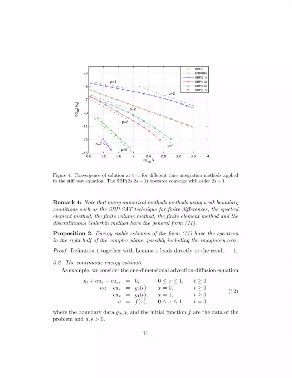
Figure 4: Convergence of solution at t=1 for different time integration methods appliedto the stiff test equation. The SBP(2s,2s− 1) operator converge with order 2s− 1.

Remark 4: Note that many numerical methods methods using weak boundaryconditions such as the SBP-SAT technique for finite differences, the spectralelement method, the finite volume method, the finite element method and thediscontinuous Galerkin method have the general form (11).

Proposition 2. Energy stable schemes of the form (11) have the spectrumin the right half of the complex plane, possibly including the imaginary axis.

Proof. Definition 1 together with Lemma 1 leads directly to the result.

3.2. The continuous energy estimate

As example, we consider the one-dimensional advection-diffusion equation

ut + aux − ǫuxx = 0, 0 ≤ x ≤ 1, t ≥ 0au− ǫux = g0(t), x = 0, t ≥ 0

ǫux = g1(t), x = 1, t ≥ 0u = f(x), 0 ≤ x ≤ 1, t = 0,

(12)

where the boundary data g0, g1 and the initial function f are the data of theproblem and a, ǫ > 0.

11

By multiplying (12) with u and integrating in space we obtain,

||u||2t+2ǫ||ux||2 = a−1

[

(au− ǫux)2 − (ǫux)

2]

x=0−a−1

[

(au− ǫux)2 − (ǫux)

2]

x=1

where ||u||2 =∫

1

0u2dx and ||ux||

2 =∫

1

0u2

xdx. Next we insert the boundaryconditions and arrive at the continuous energy rate

||u||2t + 2ǫ||ux||2 = a−1

[

g20+ g2

1− (au− g0)

2 − (au− g1)2]

. (13)

Finally, by time integration, we have the result for the continuous problem

||u(·, T )||2 + 2ǫ∫ T

0||ux(·, t)||

2dt = ||f ||2 + a−1∫ T

0[g2

0+ g2

1] dt

− a−1∫ T

0[(au− g0)

2 + (au− g1)2] dt.

(14)

Note that the norm of the solution at the final time and the time integralof the first derivative is bounded by initial data and boundary data. Theestimate (14) is the target for the fully discrete energy estimate that we willderive below.

3.3. The semi-discrete energy estimate

The semi-discrete approximation of (12) using the SBP-SAT technique is

Ut + aDU − ǫD2U = P−1(σ0(L0U − g0)~e0 + σN(LNU − g1) ~eN)U(0) = F0,

(15)

where D = P−1Q, L0U = aU0 − ǫ(DU)0, LNU = ǫ(DU)N and ~eN =(0, 0, ..., 0, 1)T . The vector U(t) = (U0(t), U1(t), ..., UN−1, UN(t))

T containsthe numerical approximation of u at all grid points in space and F0 =(f0, f1, ..., fN−1, fN)

T . The right hand side of (15) implements the bound-ary conditions weakly using the SAT technique.

By multiplying (15) with UTP from the left, using the SBP properties(4) and σ0 = σN = −1 we obtain the semi-discrete energy rate

||U ||2t + 2ǫ||DU ||2 = a−1[

g20+ g2

1− (aU0 − g0)

2 − (aUN − g1)2]

, (16)

where ||U ||2P = UTPU and ||DU ||2P = (DU)TP (DU). Note that the semi-discrete energy rate (16) is almost identical to the corresponding continuous(13) one. Finally, by time integration, we have the result for the semi-discreteproblem

||U(·, T )||2 + 2ǫ∫ T

0||DU(·, t)||2dt = ||F0||

2 + a−1∫ T

0[g2

0+ g2

1] dt

− a−1∫ T

0[(aU0 − g0)

2 + (aUN − g1)2] dt.

(17)

12

The similarity of the semi-discrete estimate (17) with the continuous estimate(14) is striking and demonstrates the strength of the SBP-SAT method inspace.

For future use, we rearrange the formulation (15) with σ0 = σN = −1 to

Ut + P−1RxU = P−1GU(0) = F0,

(18)

where

Rx = a(Q+ E0)− ǫ(Q+ E0 − E1)D, G = (g0, 0, ..., 0, g1)T . (19)

We have showed in (16) that (let g0 = g1 = 0)

Rx +RTx = a(E0 + EN) + 2ǫDTPD ≥ 0. (20)

Clearly now the approximation (18) is energy stable since Definition 1 holds.

3.4. The fully discrete energy estimate

Here it is convenient to introduce the Kronecker product A⊗B for arbi-trary matrices A ∈ Rm×n and B ∈ Rp×q as

A⊗ B =

a1,1B . . . a1,mB...

. . ....

an,1B . . . am,nB

. (21)

The Kronecker product is bilinear, associative and obeys the mixed productproperty

(A⊗ B)(C ⊗D) = (AC ⊗ BD) (22)

if the usual matrix products are defined. For inversion and transposing wehave

(A⊗ B)−1,T = A−1,T ⊗ B−1,T (23)

if the usual matrix inverse is defined.The fully discrete version of (12) is obtained by discretizing (15) or equiv-

alently (18) in time using the SBP-SAT technique. The use of the Kroneckerproduct rules (21-23) and (19) yield

(P−1

t Qt ⊗ Ix)U + (It ⊗ P−1

x Rx)U = (It ⊗ P−1

x )G+ σt(P

−1

t E0 ⊗ Ix)(U − F ),(24)

13

where the first index correspond to time and the second to space. We haveindicated the operators and vectors that belong to t, x with subscripts whereappropriate. The second penalty term on the right hand side include the un-known coefficient σt which will be determined for stability. The organisationof the vectors in (24) are

U = (U0, U1, ..., UM)T , Ui = (Ui0, Ui1, ..., UiN)T

G = (G0, G1, ..., GM)T , Gi = (g0(i∆t), 0, ..., 0, g1(i∆t))T

F = (F0, U1, ..., UM)T , F0 = (f0, f1, ..., fN)T

U0 = (U00, U10, ..., UM0)T , G0 = (g0(0), g0(∆t), ..., g0(M∆t))T

UN = (U0N , U1N , ..., UMN)T , G1 = (g1(0), g1(∆t), ..., g1(M∆t))T .

By multiplying (24) with UT (Pt ⊗Px) from the left, using the SBP prop-erties (4), the relation (18), the Kronecker product rules (21-23) and thechoice σt = −1 we obtain

UTMPxUM + 2ǫ(DU)T (Pt ⊗ Px)DU = F T

0PxF0

+ a−1[

(G0)TPtG0 + (G1)TPtG

1]

− a−1(aU0 −G0)TPt(aU0 −G0)

− a−1(aUN −G1)TPt(aUN −G1)

− (U0 − F0)TPx(U0 − F0).

(25)

Note the close similarity between the continuous estimate (14), the semi-discrete estimate (17) and the fully discrete one in (25). The fully discreteestimate has the additional damping term −(U0 −F0)

TPx(U0 −F0) from thetime-discretisation, also present in (7).

By rearranging (24), we get the final equation to solve for U

BU = (Bt +Bx)U =[

(P−1

t Qt ⊗ Ix) + (It ⊗ P−1

x Rx)]

U = H, (26)

where Qt = Qt−σtE0, Rx is defined in (19) andH = (It⊗P−1

x )G−σt(P−1

t E0⊗Ix)F is the data vector.

For example, by using the second order operator in (5), the matrix B in(26) becomes:

B =

−1−2σ△x

Ix + P−1

x Rx1

△xIx

− 1

2△xIx P−1

x Rx1

2△xIx

. . . . . . . . .

− 1

2△xIx P−1

x Rx1

2△xIx

− 1

△xIx

1

△xIx + P−1

x Rx

.

14

For higher order of accuracy in time, the banded structure of B becomeswider and with higher order in space, the bandwidth of Rx becomes larger.The size of the blocks Ix and P−1

x Rx increase with higher resolution in space.The following theorem will be needed.

Theorem 1. Let A and B be two matrices. If A and B commute, they aresimultaneously triangularizable, i.e. there exists a unitary matrix X such thatA = XTAX

∗ and B = XTBX∗, where TA and TB are both upper triangular.

Proof. See for example the proof of theorem 40.4 in [40].

We will also need the following Lemma.

Lemma 2. The matrices Bt and Bx commute, i.e. BtBx = BxBt.

Proof. Let Ct = P−1

t Qt and Cx = P−1

x Rx. We have BtBx = (Ct ⊗ Ix)(It ⊗Cx) = (Ct ⊗ Cx) = (It ⊗ Cx)(Ct ⊗ Ix) = BxBt.

We are now ready to show

Proposition 3. Given that Assumption 1 holds, then the matrix B = Bt+Bx

in (26) have eigenvalues with strictly positive real parts.

Proof. Theorem 1 and Lemma 2 leads to B = Bt + Bx = XTtX−1 +

XTxX−1 = X(Tt + Tx)X

−1 where X is unitary, and Tx and T2 are (up-per) triangular matrices. Any eigenvalue λ of B can thus be written asλ = λt + λx, where λt and λx are eigenvalues of Bt and Bx respectively. Therelation (20) and Lemma 1 show that the eigenvalues of Bx have positivesemi-definite real parts. If Assumption 1 holds, then the eigenvalues of Bt

have strictly positive real parts and the result follows.

Remark 5: Proposition 3 show that (26) has a unique bounded solution.

3.5. Numerical calculations for the initial boundary value problems

We use the method of manufactured solutions, see [41],[42],[43] to employthe exact solution u = sin(2π(x − t)) for the advection-diffusion problem(12). The boundary conditions are imposed with the standard SBP − SATtechnique and data from the exact solution. As was mentioned above, inthe present calculations, we used the linear equations solver (”backslash”) inMATLAB.

15

2 3 4 5 6 7 8 9−20

−15

−10

−5

0

5

10

15

20

Re(λ)

Im(λ

)

Figure 5: The spectrum of the non-stiff advection-diffusion problem using a second orderspatial discretization with ∆x = 1/16. The real part of the eigenvalues are strictly positive.

As a non-stiff case we use the parameters a = 1, ǫ = 0.01. We use asecond order coarse (∆x = 1/16) spatial discretization. Figure 5 shows theeigenvalue distribution of the semi-discrete problem, while Figure 7 showsconvergence to the exact solution of the semi-discrete problem. The exactsolution of the semi-discrete problem was obtained by using a very fine timeintegration scheme. The convergence rates are approximately 2s, just as wesaw with the non-stiff initial value problem in section 2.4.1.

Next we consider a stiff IBVP calculation by choosing a = 1 and ǫ = 10.This time we use an eighth order, high resolution (∆x = 0.01) spatial dis-cretization to make sure that the error in the fully discrete solution is domi-nated by the temporal discretization. Figure 6 shows the semi-discrete spec-trum of this problem and it can be seen by comparing with the spectrum inFigure 5 that the problem is indeed stiff. Figures 8 and 9 show the conver-gence to the exact solution. We see that ESDIRK4 shows order reductionalso in this case, especially in the lower range of temporal resolution. TheSBP (2s, s) methods show convergence rates between s and s + 1 for lowerresolution, while the SBP (2s, 2s−1) methods converge with orders between

16

100

101

102

103

104

105

106

107

−200

−150

−100

−50

0

50

100

150

200

Re(λ)

Im(λ

)

Figure 6: The spectrum of the stiff advection-diffusion problem using an eighth orderspatial discretization with ∆x = 0.01. The real part of the eigenvalues are strictly positive.

2s− 1 and 2s. In the latter case, the order reduction is minor for the higherorder methods, if at all present. Note also the similarities between theseresults and those in section 2.4.2.

We conclude that block norms should be favored over diagonal normswhenever possible, due to the relatively minor order reduction experiencedin the stiff case. We also stress that the practical efficiency of the SBP−SATtechnique will greatly depend on the technique used to solve the large linearequation system arising from the spatial and temporal discretization.

4. The initial boundary value problem for systems of equations

The stability theory in section 3.4 above can be extended to all energystable semi-discrete systems of equations in multiple dimensions. Such energystable semi-discrete approximations can for example be found in [24, 22, 23,25, 26, 27, 28, 29, 30, 31] where the SBP-SAT technique in space was used.However, the methodology is completely general and suitable for all semi-discrete energy stable problems. We consider formulations on the form (11)such that we have an energy stable approximation, see Definition 1. The

17

0.8 1.2 1.6 2 2.4−15

−13

−11

−9

−7

−5

−3

−1

0

log10

Nt

log

10||e

Nt||

SBP(2,1)

SBP(4,2)

SBP(4,3)

SBP(6,3)

SBP(6,5)

SBP(8,4)

SBP(8,7)

p=2

p=6

p=8

p=4

Figure 7: Temporal convergence in the discrete L2 norm at t = 1 for the non-stiff advection-diffusion equation. Results for SBP(2s,s) and SBP(2s,2s-1) operators are shown.

ambition in this section is to give an overview of the general stability theory,and hence some details will not be scrutinized.

The multi-dimensional fully discrete approximation analogous to (24) is

(P−1

t Qt⊗Is)U+(It⊗P−1R)U = (It⊗P−1)G+σt(P−1

t E0⊗Is)(U−F ). (27)

The first index correspond to time and the second one is a multi-index corre-sponding to the number of dimensions in space and the number of equationsin the system. The vectors G and F are the boundary and initial data orga-nized in an appropriate way (F now contains the initialdata F0). The matrixIs is the identity matrix for the multi-index. The energy method applied to(27) and the choice σt = −1 yield

UTMPsUM ≤ F T

0PsF0 − (U0 − F0)

TPs(U0 − F0), (28)

which correspond to (25) in the fully discrete one-dimensional case.Remark 6: The estimate (28) above means that systems like the Maxwells’equations, the elastic wave equations and the linearized Euler and Navier-Stokes equations can be shown to be stable for fully discrete high order ap-

18

0.8 1.2 1.6 2 2.4 2.8−11

−10

−9

−8

−7

−6

−5

−4

−3

−2

−1

log10

Nt

log

10||e

Nt||

BDF2

ESDIRK4

SBP(2,1)

SBP(4,2)

SBP(6,3)

SBP(8,4)

p=5

p=1

p=2

p=4

p=3

Figure 8: Temporal convergence in the discrete L2 norm at t = 1 for the stiff advection-diffusion equation. Results for BDF2, ESDIRK4 and SBP(2s,s) operators are shown.

proximations. Stability is obtained in an almost automatic way if the systemsare energy stable in a semi-discrete sense.

5. Conclusions

We develop a new high order accurate time-integration technique for ini-tial value problems by extending the well known SBP-SAT technique forspace discretisation into the time domain. We use summation-by-parts op-erators in time and a weak initial condition.

The new time-integration method is global, high order accurate, uncondi-tionally stable and together with energy stable semi-discrete approximations,it generates optimal fully discrete energy estimates. Even though we focus onfinite difference approximations, we stress that the methodology is completelygeneral and suitable for all semi-discrete energy-stable approximations.

We have derived optimal energy estimates for the scalar initial value prob-lem, the scalar advection-diffusion problem and done numerical experiments.The experiments verify that the SBP-SAT schemes in time are comparableto and sometimes better than other popular methods.

19

0.8 1.2 1.6 2 2.4 2.8−11

−10

−9

−8

−7

−6

−5

−4

−3

−2

−1

log10

Nt

log

10||e

Nt||

BDF2

ESDIRK4

SBP(2,1)

SBP(4,3)

SBP(6,5)

SBP(8,7)

p=1

p=6

p=8

p=2

p=4

p=3

Figure 9: Temporal convergence in the discrete L2 norm at t = 1 for the stiff advection-diffusion equation. Results for BDF2, ESDIRK4 and SBP(2s,2s-1) operators are shown.

The theoretical work on the initial value problem and the scalar advection-diffusion problem was generalized to energy stable multi-dimensional systemproblems such as the Maxwells’ equations, the elastic wave equations andthe linearized Euler and Navier-Stokes equations. It was shown how fullydiscrete energy estimates for high order approximations can be obtained inan almost automatic way.

In this paper we focused on the excellent stability properties of themethod. Future work will include work on how to construct an efficientsolution procedure. Also, we have considered constant coefficient problems.Time-dependent coefficients and nonlinear problems will be a future topic aswell.

References

[1] J. Butcher, Numerical Methods for Ordinary Differential Equations,John Wiley & Sons, Ltd.

20

[2] M. Spijker, Stiffness in numerical initial-value problems, Journal ofComputational and Applied Mathematics 72 (1996) 393–406.

[3] J. R. Cash, Modified extended backward differentiation formulae forthe numerical solution of stiff initial value problems in odes and daes,Journal of Computational and Applied Mathematics 125 (2000) 117–130.

[4] J. R. Cash, The integration of stiff initial value problems in odes usingmodified extended backward differentiation formulae, Computers andMathematics with Applications 9 (1983) 645–657.

[5] C. A. Kennedy, M. H. Carpenter, Additive runge-kutta schemes forconvection-diffusion-reaction equations, Applied Numerical Mathemat-ics 44 (2003) 139–181.

[6] M. H. Carpenter, C. A. Kennedy, H. Bijl, S. A. Viken, V. N. Vatsa,Fourth-order runge-kutta schemes for fluid mechanics applications,Journal of Scientific Computing 25 (2005) 157–194.

[7] W. Hundsdorfer, S. J. Ruuth, On monotonicity and boundedness prop-erties of linear multistep methods, Mathematics of Computation 75(2006) 655–672.

[8] W. Hundsdorfer, A. Mozartova, M. N. Spijker, Stepsize restrictionsfor boundedness and monotonicity of multistep methods, Journal ofScientific Computing 50 (2012) 265–286.

[9] J. C. Butcher, Initial value problems: numerical methods and mathe-matics, Computers and Mathematics with Applications 28 (1994) 1–16.

[10] J. C. Butcher, General linear methods for stiff differential equations,BIT Numerical Mathematics 41 (2001) 240–264.

[11] W. Hundsdorfer, S. J. Ruuth, Imex extensions of linear multistep meth-ods with general monotonicity and boundedness properties, Journal ofComputational Physics 225 (2007) 2016–2042.

[12] A. Kanevsky, M. H. Carpenter, D. Gottlieb, J. S. Hesthaven,Application of implicit-explicit high order runge-kutta methods todiscontinuous-galerkin schemes, Journal of Computational Physics 225(2007) 1753–1781.

21

[13] O. Axelsson, Global integration of differential equations through lobattoquadrature, BIT 4 (1964) 69–86.

[14] F. Costabile, A. Napoli, A method for global approximation of the initialvalue problem, Numerical Algorithms 27 (2001) 119–130.

[15] B. Guo, Z. Wang, Legendre-Gauss collocation methods for ordinary dif-ferential equations, Advances in Computational Mathematics 30 (2009)249–280.

[16] Z. Wang, B. Guo, Legendre-gauss-radau collocation method for solv-ing initial value problems of first order ordinary differential equations,Journal of Scientific Computing (2011) 1–30. Article in Press.

[17] H.-O. Kreiss, G. Scherer, Finite element and finite difference methods forhyperbolic partial differential equations, in: C. De Boor (Ed.), Math-ematical Aspects of Finite Elements in Partial Differential Equation,Academic Press, New York, 1974.

[18] B. Strand, Summation by parts for finite difference approximation ford/dx, Journal of Computational Physics 110 (1994) 47–67.

[19] M. Carpenter, J. Nordstrom, D. Gottlieb, A stable and conservativeinterface treatment of arbitrary spatial accuracy, Journal of Computa-tional Physics 148 (1999) 341–365.

[20] K. Mattsson, J. Nordstrom, Summation by parts operators for finite dif-ference approximations of second derivatives, Journal of ComputationalPhysics 199 (2004) 503–540.

[21] M. H. Carpenter, D. Gottlieb, S. Abarbanel, Time-stable boundary con-ditions for finite-difference schemes solving hyperbolic systems: Method-ology and application to high-order compact schemes, Journal of Com-putational Physics 111 (1994) 220–236.

[22] M. Svard, M. Carpenter, J. Nordstrom, A stable high-order finite dif-ference scheme for the compressible Navier-Stokes equations: far-fieldboundary conditions, Journal of Computational Physics 225 (2007)1020–1038.

22

[23] M. Svard, J. Nordstrom, A stable high-order finite difference schemefor the compressible Navier-Stokes equations: No-slip wall boundaryconditions, Journal of Computational Physics 227 (2008) 4805–4824.

[24] K. Mattsson, M. Svard, M. Carpenter, J. Nordstrom, High-order accu-rate computations for unsteady aerodynamics, Computers and Fluids36 (2007) 636–649.

[25] J. E. Kozdon, E. M. Dunham, J. Nordstrom, Interaction of waveswith frictional interfaces using summation-by-parts difference operators:Weak enforcement of nonlinear boundary conditions, Journal of Scien-tific Computing 50 (2012) 341–367.

[26] J. E. Kozdon, E. M. Dunham, J. Nordstrom, Simulation of dynamicearthquake ruptures in complex geometries using high-order finite dif-ference methods, Journal of Scientific Computing (2012) 1–33.

[27] J. Berg, J. Nordstrom, Stable Robin solid wall boundary conditionsfor the Navier-Stokes equations, Journal of Computational Physics 230(2011) 7519–7532.

[28] J. Nordstrom, J. Gong, E. van der Weide, M. Svard, A stable andconservative high order multi-block method for the compressible navier-stokes equations, Journal of Computational Physics 228 (2009) 9020–9035.

[29] J. Nordstrom, R. Gustafsson, High order finite difference approxima-tions of electromagnetic wave propagation close to material discontinu-ities, Journal of Scientific Computing 18 (2003) 215–234.

[30] J. Nordstrom, J. Berg, Conjugate heat transfer for the unsteady com-pressible Navier-Stokes equations using a multi-block coupling, Com-puters and Fluids 72 (2013) 20–29.

[31] J. Nordstrom, S. Eriksson, P. Eliasson, Weak and strong wall boundaryprocedures and convergence to steady-state of the navier-stokes equa-tions, Journal of Computational Physics 231 (2012) 4867–4884.

[32] M. Svard, On coordinate transformations for summation-by-parts op-erators, Journal of Scientific Computing 20 (2004) 29–42.

23

[33] J. Nordstrom, Conservative finite difference formulations, variable coef-ficients, energy estimates and artificial dissipation, Journal of ScientificComputing 29 (2006) 375–404.

[34] J. Nordstrom, Error bounded schemes for time-dependent hyperbolicproblems, SIAM Journal on Scientific Computing 30 (2007) 46–59.

[35] J. E. Hicken, D. W. Zingg, Superconvergent functional estimates fromsummation-by-parts finite-difference discretizations, SIAM Journal onScientific Computing 33 (2011) 893–922.

[36] J. Berg, J. Nordstrom, Superconvergent functional output for time-dependent problems using finite differences on summation-by-partsform, Journal of Computational Physics 231 (2012) 6846–6860.

[37] J. Berg, J. Nordstrom, On the impact of boundary conditions on dualconsistent finite difference discretizations, Journal of ComputationalPhysics 236 (2013) 41–55.

[38] A. Prothero, A. Robinson, On the stability and accuracy of one-stepmethods for solving stiff systems of ordinary differential equations, SiamJournal on Scientific Computing 28 (1974) 145–162.

[39] K. Burrage, L. Petzold, On order reduction for runge-kutta methodsapplied to differential/ algebraic systems and to stiff systems of odes,SIAM Journal on Numerical Analysis 27 (1990) 447–456.

[40] V. Prasolov, Problems and Theorems in Linear Algebra, AmericanMathematical Society, 1994.

[41] P. J. Roache, Code verification by the method of manufactured solu-tions, Journal of Fluids Engineering, Transactions of the ASME 124(2002) 4–10.

[42] L. Shunn, F. Ham, P. Moin, Verification of variable-density flow solversusing manufactured solutions, Journal of Computational Physics 231(2012) 3801 – 3827.

[43] J. Lindstrom, J. Nordstrom, A stable and high-order accurate conjugateheat transfer problem, Journal of Computational Physics 229 (2010)5440–5456.

24