Superconductivity with excitons and polaritons

F. P. Laussy,1, ∗ T. Taylor,1 I. A. Shelykh,2, 3 and A. V. Kavokin1

1School of Physics and Astronomy, University of Southampton, Highfield, Southampton, SO17 1BJ, UK.2Science Institute, University of Iceland, Dunhagi-3, IS-107, Reykjavik, Iceland.

3International Institute for Physics, Av. Odilon Gomes de Lima,1722, CEP: 59078-400, Capim Macio, Natal RN Brazil.

A Bose–Einstein condensate of exciton polaritons coexisting with a Fermi gas of electrons hasbeen recently proposed as a promising system for realisation of room-temperature superconductiv-ity [Phys. Rev. Lett., 104, 106402 (2010)]. In order to find the optimum conditions for exciton andexciton-polariton mediated superconductivity, we study the attractive mechanism between electronsof a Cooper pair mediated by the exciton and exciton-polariton condensate and analyze the gapequation that follows. We specifically address microcavities with embedded n-doped quantum wellsas well as coupled quantum wells hosting a condensate of spatially indirect excitons, put in contactwith a two-dimensional electron gas. We show that engineering of the interaction in these peculiarBose-Fermi mixtures is complex and sometimes counterintuitive, but leaves much freedom for op-timization, making promising the realization of high-temperature superconductivity in multilayersemiconductor structures.

PACS numbers: 71.35.Gg, 71.36.+c, 71.55.Eq, 74.78.-w, 74.90.+n

∗ Presently at Walter Schottky Institut, Technische Universitat Munchen, Am Coulombwall, 3 D-85748, Garching, Germany.

arX

iv:1

102.

1484

v1 [

cond

-mat

.sup

r-co

n] 8

Feb

201

1

2

I. INTRODUCTION

The electron gas undergoes, in some conditions, a phase transition to bound pairs of electrons (the so-calledCooper pairs), that replace electrons as the fundamental agent of the electronic properties. The Cooper pairs are,from the point of view of their electric charge, objects qualitatively identical to the underlying electrons. From thepoint of view of their spin, on the other hand, they become integer-spin particles, that is, from the spin-statisticstheorem, bosons rather than fermions. This shift of statistical paradigm of the carriers, from Fermi to Bose-statistics,results in the outstanding behaviour of superconductivity, that is, conduction of electric charge by a macroscopiccoherent wavefunction (akin to a Bose-Einstein condensate). It has taken some time to capture the fundamental anduniversal features of this phenomenon and set them apart from particularities proper to certain cases only. The gap ofexcitations, responsible for zero resistivity, for instance, results from the long-range nature of the Coulomb interaction,but gapless superconductivity is also possible. One of the central, fundamental concepts of superconductivity is thatof a coherent quantum state of charged bosons. Although superconductivity was discovered empirically, and itstheoretical construction consisted in assembling a puzzle, it is now possible to envisage engineering superconductingphases in other systems, based on this understanding of condensation of charged bosons. If superconducting phasescan be identified in other systems, progresses will be quick for the understanding of cuprate superconductivity, whichstill eludes compelling theoretical explanation of its intrinsic mechanism.

A system that is making rapid and impressive progress in terms of creating and controlling macroscopic quantumstates is that of microcavity exciton-polaritons [1] (see [2] for a review). These quasi-particles that combine propertiesof light (cavity photons) and matter (quantum well excitons) have been noted for their predisposition to accumulatein macroscopic number in a single or few quantum states [3, 4]. They have many advantages from a practical pointof view, such as their 2D geometry, which allows straightforward manipulation by lasers impinging at an angle, andtheir short lifetime, which allows continuous monitoring of the system, reconstructing its internal dynamics alsoby angle-resolved spectroscopy [5]. The pumping can be either coherent (driving states in parametric scatteringconfigurations) [6–10] or incoherent (with a constant flow of unrelated particles relaxing into the ground state ) [11–16]. In nitride systems, the formidable claim has been made of room temperature Bose-Einstein condensation [17, 18].Recently, there has been great interest in propagation of polariton fluids [19, 20] and their superfluid properties [21],with reports of quantized vorticity [22, 23] and persistent currents [24].

These rising stars of macrosopic coherence have also been proposed to service another much sought after quantumphase at high temperature: superconductivity. Polariton condensates cannot conduct electric current themselves,being neutral particles. One of the proposed implementations involves “quatrons” (or quadrions) rather than po-laritons [25]. Quatrons are bound states of two electrons with a polariton. They remain bosons from spin-additionrules but carry an electric charge. A Bose condensate of quatrons would, through its superfluid propagation, exhibitsuperconductivity. To date, however, the existence of the quatron, predicted theoretically [25], has not been foundexperimentally. Recently, we have approached the problem from another, and more conventional, angle, that of theBCS mechanism [26] with an important new feature: replacement of phonons by Bose-condensed exciton-polaritonsin the role of a binding agent between electrons. In the present paper, we generalise the model proposed in [26] todescribe a wide range of hybrid Bose-Fermi semiconductor systems where a Bose-Einstein condensate of neutral quasi-particles (excitons or exciton-polaritons) coexists with a Fermi sea of electrons. We show that indeed such systemsare promising for observation of (high-temperature) superconductivity. Moreover, as the superconducting gap andcritical temperature appear to be very sensitive to the concentration of bosons in the system and the latter may becontrolled by direct optical excitation of exciton, light induced superconductivity in semiconductor heterostructuresappears to be possible. In this work we closely follow the BCS approach, generalised and adapted to the case ofsuperconductivity mediated by a Bose-Einstein condensate. Solving the gap equation in this case turns out to be anon-trivial problem, requiring careful analysis.

A. BCS with a Bose-Einstein condensate as a binding agent

BCS is a pillar of superconductivity theory, which relies on three main tenets:

1. Instability of the Fermi sea,

2. Existence of an attractive interaction,

3. Condensation of charged bosons.

These are the three insights that were mainly contributed by Cooper, Bardeen and Schrieffer, respectively, and thatthey could assemble into the BCS theoretical edifice and exploit to reproduce strikingly or predict successfully mostof the superconductivity phenomenology.

3

The first point follows from Cooper’s observation [27] that an arbitrary small attractive interaction between twoelectrons on top of the Fermi sea leads to a bound state (the Cooper pair), thanks to the truncation of the momentumspace for states with wavevector k > kF (Fermi wavevector). This is a general result, that follows from Bethe-Goldstoneequation for the two-electron problem.

The second point is the identification of an effective attraction between electrons that normally experience bareCoulomb repulsion. This attraction is attributed for conventional superconductors to an interaction through phonons,the Bardeen-Pines potential [28], that consists, vividly, of one electron wobbling the lattice at a first time, which affectsanother electron at a second time (and at a larger timescale, since the lattice dynamics is much slower than that ofelectrons) [29]. If the frequency of the lattice vibration is smaller than that of the propagating electron, the net effectresults in an effective attraction [Leggett offers an insightful toy model of coupled oscillators to capture the essenceof the interaction character (attractive or repulsive) [30]].

The last point is the so-called BCS state, which is a coherent superposition of paired bound states and which bringsthe two-particle Cooper effect to a collective behaviour of all electrons in the system [31].

With these three ingredients put together, the BCS theory is complete [32]. For our purposes, points 1 and 3 willbe regarded as fundamental and well established features of (BCS type of) superconductivity. Point 2, that mightappear a mere desiderata for point 1 to apply, leaves us room for identifying and designing new types of attractivepotentials, optimizing the range of applicability and strength so as to obtain robust superconductivity (e.g., holding athigh temperatures or high magnetic fields) or its manifestation in a new class of systems (in microcavities). Bardeenhimself, with coworkers [33], investigated possibilities to engineer a more robust BCS in a bilayer structure whereexcitons replace phonons as mediators of the interaction. The idea of substituting phonons by excitons was pioneeredby Little [34] and developed by Ginzburg [35], who coined the term and theorized the possibility of high-temperaturesuperconductivity, much before it came to fruition with cuprates [36]. Those, however, exploit another (still unknown)mechanism different to BCS [37].

In the following, we revisit the Ginzburg mechanism, based on BCS, with emphasis on maximizing the strength ofinteraction between electrons, so as to maintain their binding, and therefore superconductivity, to higher temperatures.The text is organized as follows: in Section II, we give a short overview of the BCS mechanism and the exciton(Ginzburg) mechanism, outlining the points of special interest in our case. In particular, we introduce the gapequation. In Section III, we introduce our hybrid Bose-Fermi system configuration, its Hamiltonian and microscopicinteractions, and the effective electron-electron Hamiltonian that results from a mean field approximation for thecondensate and the usual Frolich transformation. We obtain the shape of the effective electron-electron interactionU , that we find to be quite different in character to the Cooper (square well) potential. We also consider possiblevariations of our scheme, namely, a microcavity with a condensate of exciton-polaritons and a condensate of indirectexcitons in coupled quantum wells [38]. The system of coupled quantum wells explored by several groups [39, 40] mightbe easier to realize and study (it does not need a cavity) and presents some interesting differences as compared to thepolariton system. On the other hand, polaritons condense at much higher temperatures [18]. In Section IV, we studythe gap equation for a Bose condensate mediated effective interaction. Because the potential is not positive-definite,the problem is not well-posed numerically. We propose a simplified potential and an approximate solution of thegap equation, that we motivate by studying its validity on well-established approximations. We obtain the criticaltemperature in this case. In Section V, we give our conclusions and perspective on this new application of excitonsand polaritons and discuss how to measure the effect experimentally.

II. BCS AND GINZBURG MECHANISMS

Superconductivity is a fundamental property of solids. At low enough temperatures, most metals superconduct.As the mechanism is rooted in quantum mechanics, temperatures are expected to be very low and indeed this isthe case for all metals. After considerable theoretical efforts from various groups, a compelling theoretical modelwas assembled by Bardeen, Cooper and Schrieffer, the so-called BCS theory [29]. The model provides the criticaltemperature:

kBTC = Θe−1g (1)

where, in conventional superconductivity, ~ωD is the Debye energy, and g = N (0)V with N (0) the density of electronsat the Fermi energy and V the electron-phonon coupling strength. The Debye energy is, in good approximation, themaximum energy that can be carried by a phonon. The mechanism therefore relies heavily on phonons, as wasrealized empirically before the advent of BCS (good conductors, for instance, are bad superconductors, since V issmall, or through the isotope effect, which correlates critical temperature with weight of the crystal atoms, and thuswith resonance frequency). The exponential form and the presence of N (0) show that the effect is a collective one

4

involving all electrons, which have formed a new phase of matter that cannot be approached perturbatively by theindependent electron pictures (since f(z) = e−1/z has no Taylor expansion around zero). Based on the theory, andaccumulated experience, it was widely accepted that critical temperatures would not exceed a few tens of Kelvins,since the Debye energy, which can be quite large in some systems (hundreds of Kelvins), is exponentially reduced. Inall conventional superconductors N (0)V � 1 (the so-called weak-coupling regime).

Ginzburg made the obvious but daring assumption that to achieve higher critical temperatures—crucial for technicalapplications which can easily be understood to be momentous—it is enough to find a system where Θ and/or g areincreased. Replacing phonons by excitons, for instance, Ginzburg found that values Θ ≈ 103, 104K as well as g ≈ 1

5 ,13 are obtained, yielding temperatures of several hundred Kelvin [41]. High critical temperatures have been laterreported in cuprates [36] and nowadays, temperatures as high as 125K are reported in systems such as Tl-Ba-Cu-oxide. Just as superconductivity in metals was discovered ahead of theory, cuprate superconductivity does not appearto follow the BCS pattern [42] even with substitution of the mediating field as proposed by Ginsburg. All attemptsto date to realize the exciton mechanism or a variation of it have remained fruitless, but it is this mechanism, rootedin BCS, which we consider in this text. Before we turn to the mechanism we propose, which consists in substitutingthe phonons of conventional BCS, or the excitons of Ginzburg scheme, by a Bose-Einstein condensate (BEC) ofexcitons or exciton-polaritons, we recall that the starting point of a microscopic derivation of superconductivity is thegap-equation:

∆k = −∑k′

Ukk′∆′k2E

(2)

where Ukk′ is the effective interaction between electrons with wavevectors k and k′ and energy E. The gap ∆ can beidentified as the macroscopic wavefunction of a Cooper pair, which is also the order parameter for the superconductingphase. If it is nonzero, the system is in the superconducting state. A realistic microscopic treatment of U is verycomplicated. A simplified version is provided by the Jellium model, which is a toy model of a metal that givespredominance to electron-electron interactions, that is, in particular, the underlying crystal is approximated as auniform (structureless) background (like a “jelly”) in which the interacting electron gas evolves under its own self-interactions and the overall charge cancellation of the background. A popular effective interaction is given by theBardeen-Pines potential [30] which is derived from the microscopic form of the electron-lattice interaction:

UBP(ω,q) =κ0

1 + q2/q2TF

{1 +

ωph(q)2

ω2 − ωph(q)2

}, (3a)

=κ0

(1 + q2

κ23D

)(1− ω2i

ω2 ), (3b)

with q = k − k′. In Eq. (3a), qTF is the Thomas-Fermi screening parameter and ωph is the phonon dispersion. Thefirst term between the brackets is bare Coulomb repulsion, and the second term, which is frequency dependent, followsfrom the perturbative coupling to the lattice, tracing out the phonons.

The physical meaning of Eq. (3a) is at the heart of the phonon-mediated mechanism. The interaction is ω dependent,which means, in Fourier transform, time dependent. This reflects the famous retardation effect in superconductivity.This effect is based on the strong difference between the electron Fermi velocity in metals and the sound velocity.Roughly speaking, a fast electron from the Fermi surface creates a slow phonon and goes away. After some time,another fast electron arrives and absorbs the slow phonon. The average distance between these two electrons remainsof the order of 100nm, the distance at which the screened Coulomb repulsion can be safely neglected. Due to theretardation effect, a weak phonon-mediated attraction of electrons wins over their Coulomb repulsion and providesformation of Cooper pairs at low enough temperatures.

III. INTERACTION HAMILTONIAN

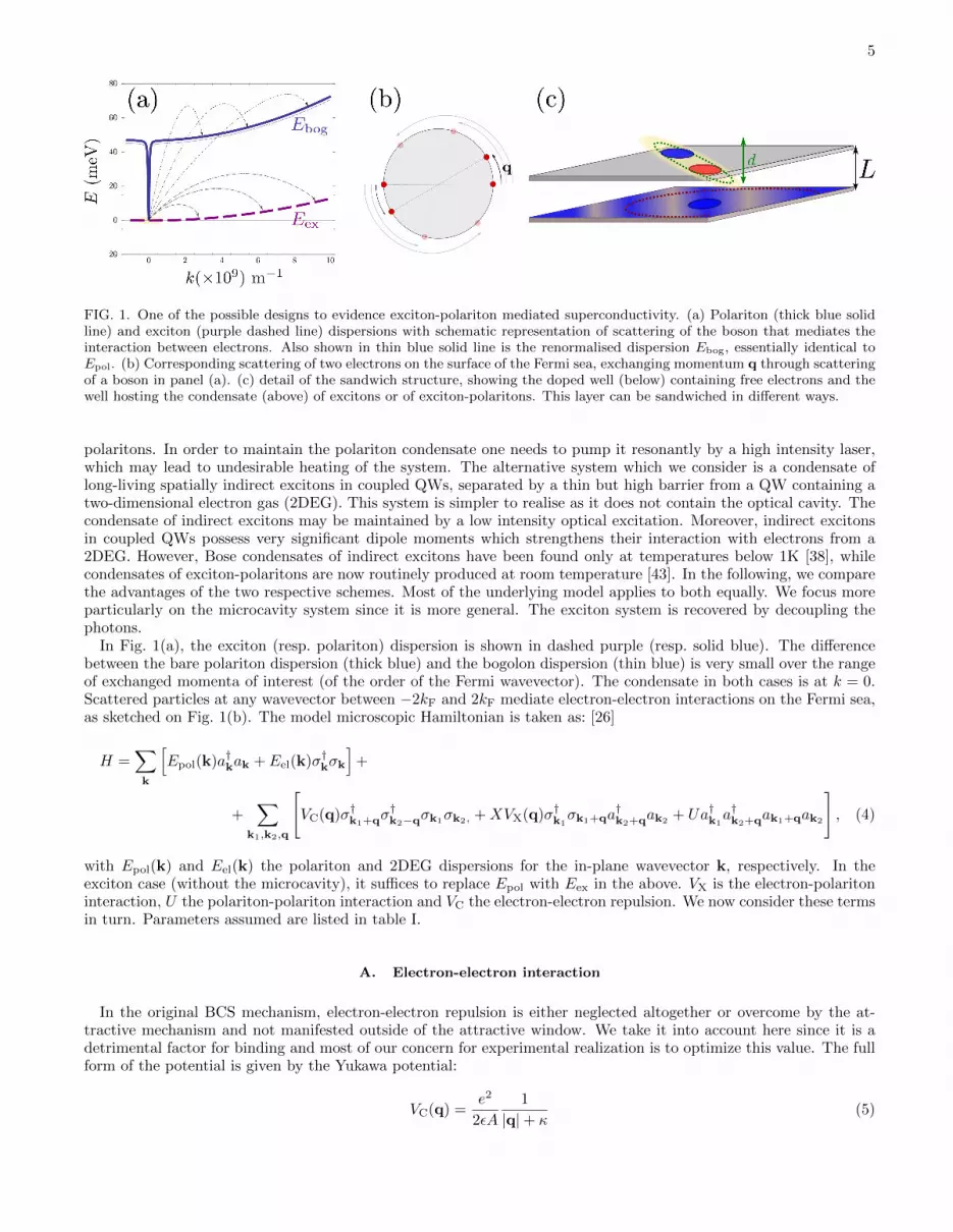
A sketch of the structure we propose appears in Fig. 1(c). A QW is doped negatively (with density of electrons n)and is put in contact with another QW where excitons are formed and are stable. The first (lower) QW hosts the2DEG which is to undergo superconductivity while the second (upper) QW hosts the condensate of excitons that isto mediate it. This structure can also be placed at the maximum of the optical field confined in a microcavity [26](formed by two Bragg mirrors facing each other). The latter configuration also has the advantage that two excitonic-QWs can sandwich the 2DEG-QW since in this case the condensate is delocalised in the entire structure thanks to thephoton fraction of the polariton. This allows an increase by a factor 2, or more if the multi-layer structure is furtherrepeated, of the densities achievable in this system. The drawback of microcavities is a short radiative lifetime of

5

FIG. 1. One of the possible designs to evidence exciton-polariton mediated superconductivity. (a) Polariton (thick blue solidline) and exciton (purple dashed line) dispersions with schematic representation of scattering of the boson that mediates theinteraction between electrons. Also shown in thin blue solid line is the renormalised dispersion Ebog, essentially identical toEpol. (b) Corresponding scattering of two electrons on the surface of the Fermi sea, exchanging momentum q through scatteringof a boson in panel (a). (c) detail of the sandwich structure, showing the doped well (below) containing free electrons and thewell hosting the condensate (above) of excitons or of exciton-polaritons. This layer can be sandwiched in different ways.

polaritons. In order to maintain the polariton condensate one needs to pump it resonantly by a high intensity laser,which may lead to undesirable heating of the system. The alternative system which we consider is a condensate oflong-living spatially indirect excitons in coupled QWs, separated by a thin but high barrier from a QW containing atwo-dimensional electron gas (2DEG). This system is simpler to realise as it does not contain the optical cavity. Thecondensate of indirect excitons may be maintained by a low intensity optical excitation. Moreover, indirect excitonsin coupled QWs possess very significant dipole moments which strengthens their interaction with electrons from a2DEG. However, Bose condensates of indirect excitons have been found only at temperatures below 1K [38], whilecondensates of exciton-polaritons are now routinely produced at room temperature [43]. In the following, we comparethe advantages of the two respective schemes. Most of the underlying model applies to both equally. We focus moreparticularly on the microcavity system since it is more general. The exciton system is recovered by decoupling thephotons.

In Fig. 1(a), the exciton (resp. polariton) dispersion is shown in dashed purple (resp. solid blue). The differencebetween the bare polariton dispersion (thick blue) and the bogolon dispersion (thin blue) is very small over the rangeof exchanged momenta of interest (of the order of the Fermi wavevector). The condensate in both cases is at k = 0.Scattered particles at any wavevector between −2kF and 2kF mediate electron-electron interactions on the Fermi sea,as sketched on Fig. 1(b). The model microscopic Hamiltonian is taken as: [26]

H =∑k

[Epol(k)a†kak + Eel(k)σ†kσk

]+

+∑

k1,k2,q

[VC(q)σ†k1+qσ

†k2−qσk1

σk2, +XVX(q)σ†k1σk1+qa

†k2+qak2

+ Ua†k1a†k2+qak1+qak2

], (4)

with Epol(k) and Eel(k) the polariton and 2DEG dispersions for the in-plane wavevector k, respectively. In theexciton case (without the microcavity), it suffices to replace Epol with Eex in the above. VX is the electron-polaritoninteraction, U the polariton-polariton interaction and VC the electron-electron repulsion. We now consider these termsin turn. Parameters assumed are listed in table I.

A. Electron-electron interaction

In the original BCS mechanism, electron-electron repulsion is either neglected altogether or overcome by the at-tractive mechanism and not manifested outside of the attractive window. We take it into account here since it is adetrimental factor for binding and most of our concern for experimental realization is to optimize this value. The fullform of the potential is given by the Yukawa potential:

VC(q) =e2

2εA

1

|q|+ κ(5)

6

Parameter Meaning Value

ε Permittivity 7ε0 ≈ 6.2 As/(mV)βe Electron reduced mass 0.22

0.22+1.25≈ 1.15

βh Hole reduced mass 1.250.22+1.25

≈ 0.85L Distance between wells 5 nmκ Coulomb screening length ≈1.2× 109 m−1

mx Exciton mass (0.22 + 1.25)me ≈ 1.3× 10−30 kgmc Photon mass 10−5me ≈ 9.1× 10−36 kg2g Rabi splitting 45 meV [0]

X Hopfield coefficient (exciton weight) 1/√

2 [1]

kF Fermi wavevector 5× 108 m−1

aB Exciton Bohr radius 1.98× 10−9 mRy Exciton Rydberg 32 meVl Dipole moment 4 nm

TABLE I. Parameters used in the numerical simulations. In square brackets, the value for the exciton case when the parameterdiffers from the polariton case, otherwise parameters have been taken the same for comparison.

x

y

z

y

x

FIG. 2. Average over the Fermi Surface, in 3D and 2D.

with screening constant κ. We get rid of the momentum dependence by averaging the potential Veff(ω,q) over theFermi surface (FS), where:

q = k1 − k2 (6)

and k1,2 are the momenta of the two interacting electrons on the FS (so that, in particular, k1 = k2 = kF), as shownin Fig. 2. In 3D, the FS is the surface of a sphere, while in 2D, it is a circle (we shall speak of surface in both cases).The vector difference is therefore joining the two end-points on the surface. If the potential has spherical symmetry(V (q) = V (q)), the average of all two vectors on the FS reduces to that where q is pinned at one point of the surface(the south pole in Fig. 2) and runs overs the FS. This average, in the particular choice of Fig. 2, is the usual polarintegration with k2 describing the surface as θ (and φ in 3D) are varied, with:

q2 = 2k2F(1 + cos θ) , (7)

from Al Kashi’s theorem, so that the average potential Veff reads, in 3D:

Veff(ω) =

∫ 2π

0

∫ π

0

Veff(q, ω)k2F sin θ dθdϕ/N , (8)

7

FIG. 3. Average electron-electron repulsion (in natural units) in the QW. This should be made as small as possible, which isobtained for higher Fermi wavevectors (for a given screening length).

where N is the normalization, i.e., the same integral where Veff is replaced by unity. This gives, in 3D:

Veff(ω) =1

2

∫ 1

−1

Veff(√

2k2F(1 + cos θ), ω)d cos θ , (9)

=1

4

∫ 4

0

Veff(kF

√ϑ, ω)dϑ , (10)

where we integrate over ϑ = 2(1 + cos θ) since this is a natural variable in Eq. (7), and, in 2D:

Veff(ω) =1

2π

∫ 2π

0

Veff(√

2k2F(1 + cos θ), ω)dθ . (11)

Our system is 2D, in which case, from Eqs. (5) and (11):

VC =e2

4πεA

∫ 2π

0

dθ√2k2

F(1 + cos θ) + κ=

e2

2πεA

π − 2 arctan 2kF√κ2−4k2F√

κ2 − 4k2F

if κ ≥ 2kF, (12)

=e2

2πεA

ln

∣∣∣∣∣∣1+2kF

/√4k2F−κ2

1−2kF

/√4k2F−κ2

∣∣∣∣∣∣√4k2

F − κ2if κ ≤ 2kF. (13)

This is plotted in Fig. 3. Since we are trying to maximize attraction, that is, minimize repulsion, systems withsmall screening length and large wavevectors should be favored (but these parameters play critically on other aspectsof the mechanism and the optimum is not compulsorily kF/κ� 1).

B. Electron-exciton interaction

The electron-exciton or exciton-polariton interaction is one of the most important ingredients of the mechanism,as it ultimately determines the shape of the effective potential. In the microcavity, an electron (from the 2DEG)interacts with a polariton (from the condensate) through its excitonic component, so this is really the electron-excitoninteraction that is to be computed, weighted by the Hopfield coefficient (the excitonic fraction) X. Let us consider,therefore, the scattering of an electron in one of the parallel QW, separated by a distance L from the QW withexcitons. The matrix element of the direct interaction between excitons and electrons reads:

VX(q) =

∫Ψ∗X(Q, re, rh)Ψ∗(k, r1)V (r1, re, rh)Ψ∗X(Q, re, rh)Ψ∗(k, r1)dr1dredrh (14)

8

0 1 2-1-2

0

1

2

3

4

5

FIG. 4. Electron-exciton interaction in the geometry of Fig. 1, decomposed as the direct interaction (dashed purple) and dipolarinteraction (solid blue) when the exciton is induced with a dipole moment d. The latter is both much larger and maximum atzero exchanged momentum.

where r1, re, rh correspond to the 2D coordinates of the 2DEG electron, the exciton electron and the exciton holerespectively. The 2DEG electron is described by a plane wave while the electron/hole in the condensate are assumedto be in the 1s bound state with plane wave center-of-mass motion:

Ψ(q, r1) =1√Aeikr1 , (15a)

Ψ∗X(Q, re, rh) =

√2

πA

1

aBUe (ze)Uh (zh) eiQ · (βere+βhrh)e−|re−rh|/aB =

√2

πA

Ue (ze)Uh (zh)

aBeiQ ·RXe−rX/aB , (15b)

where RX = βere + βhrh, rX = re − rh are in-plane coordinates of the center of mass of the exciton and relativecoordinate of electron and hole in the exciton, Ue (ze) and Uh (zh) are normal to the QW plane electron and holeenvelope functions, respectively. We also consider the existence of a dipole moment d for the exciton, which can beintrinsic to the structure, because of spatial separation of electrons and holes in coupled QWs, or (in the case ofmicrocavities) be induced by an internal piezo-electric field, or result from an externally applied electric field. Toaccount for all these possibilities, one can consider the layers of electrons and holes in the exciton shifted in thez-direction with respect to the position of the center of mass by a distance l = d/e� L. The matrix element of theinteraction is then computed to be:

Vdir(q) =e2

2εA

e−qL

q

{1

[1 + (βeqaB/2)2]3/2− 1

[1 + (βhqaB/2)2]3/2

}(16a)

+ed

2εAe−qL

{βe

[1 + (βeqaB/2)2]3/2

+βh

[1 + (βhqaB/2)2]3/2

}(16b)

where Eq. (16a) is the direct electron-exciton interaction that exists even in the absence of a dipole moment of theexciton, and Eq. (16b) is the dipolar interaction. The direct interaction vanishes at small exchanged momenta, whilethe dipolar-induced one assumes its maximum value here of 2d/(2ε0εA). Overall, the dipolar interaction is naturallymuch larger than the direct one, since the exciton is electrically neutral.1 These facts are summarized in Fig. 4.

1 Note at this point that there is an error in Ref [26] where only the direct exciton interaction has been taken into account with anincorrect power in the parenthesis, which led to an expression similar to the dipolar interaction. The direct interaction by itself turnsout to be too small to evidence superconductivity with the parameters chosen in Ref. [26], therefore a dipole moment should be inducedin this case, say by applying an external electric field, to restore the effect.

9

C. Polariton-polariton interaction

We treat the polariton-polariton interaction within the s-wave scattering approximation with strength U =6a2

BRyX2/A (where aB is the exciton Bohr radius, Ry the exciton binding energy and A the normalization area.

X is the exciton Hopfield coefficient, the square of which quantifies the exciton fraction in the exciton-polaritoncondensate) [44]. For interaction between bare excitons, X = 1. Exciton-exciton (polariton-polariton) interactionsare repulsive, in general. They result in linearization of the elementary excitation spectra, the Bogoliubov dis-persion, but its role is not crucial to the mechanism of superconductivity we discuss, since at the wavevectors ofinterest, the changes brought by this term are very small compared to the kinetic energy of non-interacting excitons(exciton-polaritons).

D. Effective interaction

We now proceed to bring our microscopic model towards a form suited to study Cooper-pairing and superconductiv-ity, that is, we apply the canonical Frohlich transformation that will result in an effective BCS hamiltonian. Just as inthe case of phonons, we start by getting rid of polaritons. We assume a condensate is formed with mean population N0.We do not consider which mechanism, coherent or incoherent, is responsible for creating and maintaining this state.We do assume, however, it is coherent and with a definite phase, so that we can apply the mean-field approximation

a†k1+qak1≈ 〈a†k1+q〉ak1

+a†k1+q〈ak1〉 and 〈ak〉 ≈

√N0Aδk,0 with N0 the density of polaritons in the condensate. This

allows us to obtain the following expression for the Hamiltonian, after diagonalizing the polariton part by means of aBogoliubov transformation (that leaves the free propagation of electrons and their direct interaction, HC, invariant):

H =∑k

Eel(k)σ†kσk +∑k

Ebog(k)b†kbk +HC +∑k,q

M(q)σ†kσk+q(b†−q + bq) (17)

where Ebog(k) describes the dispersion of the elementary excitations (bogolons) of the interacting Bose gas, which isvery close to a parabolic exciton dispersion at large k:

Ebog(k) =

√Epol(k)(Epol(k) + 2UN0A) , (18)

where Epol(k) ≡ Epol(k)− Epol(0) and with the renormalized bogolon-electron interaction strength:

M(q) =√N0AXVX(q)

√Ebog( q)− Epol(q)

2UN0A− Ebog(q) + Epol(q). (19)

The last term of Eq. (17) coincides with the Frohlich electron-phonon interaction Hamiltonian, which allows usto write an effective Hamiltonian for the bogolon-mediated electron-electron interaction. This results in an effective

interaction between electrons, of the type∑

k1,k2,qVeff(q, ω)σ†k1

σk1+qσ†k2+qσk2

. The effective interaction strength

reads Veff(q, ω) = VC(q) + VA(q, ω), with:

VA(q, ω) =2M(q)2Ebog(q)

(~ω)2 − Ebog(q)2. (20)

Equation (20) recovers the boson-mediated interaction potential obtained for a Bose-Fermi mixture of cold atomicgases [45], in the limit of vanishing exchanged wavevectors. It describes the BEC induced attraction between electrons.Remarkably, it increases linearly with the condensate density N0. This represents an important advantage of thismechanism of superconductivity with respect to the earlier proposals of exciton-mediated superconductivity [33,34, 46], as the strength of Cooper coupling can be directly controlled by optical pumping of the exciton-polaritoncondensate. The attractive potential is displayed for various exchanged energies in Fig. 5, as a function of theexchanged momentum expressed directly through the angle θ defined in the Fermi circle (cf. Fig. 2). As commentedearlier, the negative part corresponds to attraction, and the potential alternates between repulsive and attractivecharacter, obtained at different exchanged momenta. We do not want to keep track of such complicated wavevectordependence, and therefore will average the interaction over the Fermi sea. A notable feature is, for most values of ω,the presence of a pole θ0, where Ebog(

√2k2

F(1 + cos θ0)) = ~ω. As is seen in the figure, θ0 separates the attractivepart from the repulsive part. The average will bring the additional convenience of cancelling such divergencies. Wenote as well that the spectrum of excitations of the exciton BEC may be changed in the presence of the electron gas,

10

-100

-50

0

50

100

150

200

3.08 3.10 3.12 3.14 3.16 3.18 3.20

-100

-50

0

50

100

150

-150

1.50 1.52-0.015

1.56 1.58 1.60

-0.01

-0.005

0

1.54

FIG. 5. Effective electron-electron interaction as a function of the exchanged momentum q =√

2kF√

1 + cos θ on the Fermisea at energies ~ω = 40, 50 and 60meV, respectively. The potential is symmetric around π. In the first case, the wholedependency (over [0, 2π]) is shown, with a first zoom in the inset showing two poles and another the attractive region thatis of small amplitude but extends over a large range. With increasing energies, the poles recedes towards smaller values of θwith a dominating effect of the repulsive (positive) energy. In the central panel, in dashed purple, the regularized potential issuperimposed.

so that their eventual dispersion may be different Ebog [47]. This has no effect on the Cooper pairing of electronswhich we discuss here.

We therefore wish to perform the average

VA =

∫ 2π

0

VA(q, ω) dθ , (21)

where q =√

2k2F(1 + cos θ), as seen previously. Since VA is symmetric around π we perform the integral

∫ π0

only.The integral would be easily computed numerically if there were no pole. There are dedicated numerical methods tocompute principal values numerically [48, 49], but in our case, since the pole is first order, it is enough to isolate itanalytically by defining

f(θ) = (θ − θ0)VA(q(θ), ω) , (22)

so that then

VA =

∫ 2π

0

f(θ)− f(θ0)

θ − θ0dθ + f(θ0) ln

2π − θ0

θ0(23)

where f(θ0) = limθ→θ0 f(θ) and the first integral is regular (it is shown in Fig. 5 in dashed purple). The integration(average) is then straightforward and produces the results shown in Fig. (6).

If we take instead of Epol a quadratic dispersion for the excitation

Ex(k) =~2k2

2mx(24)

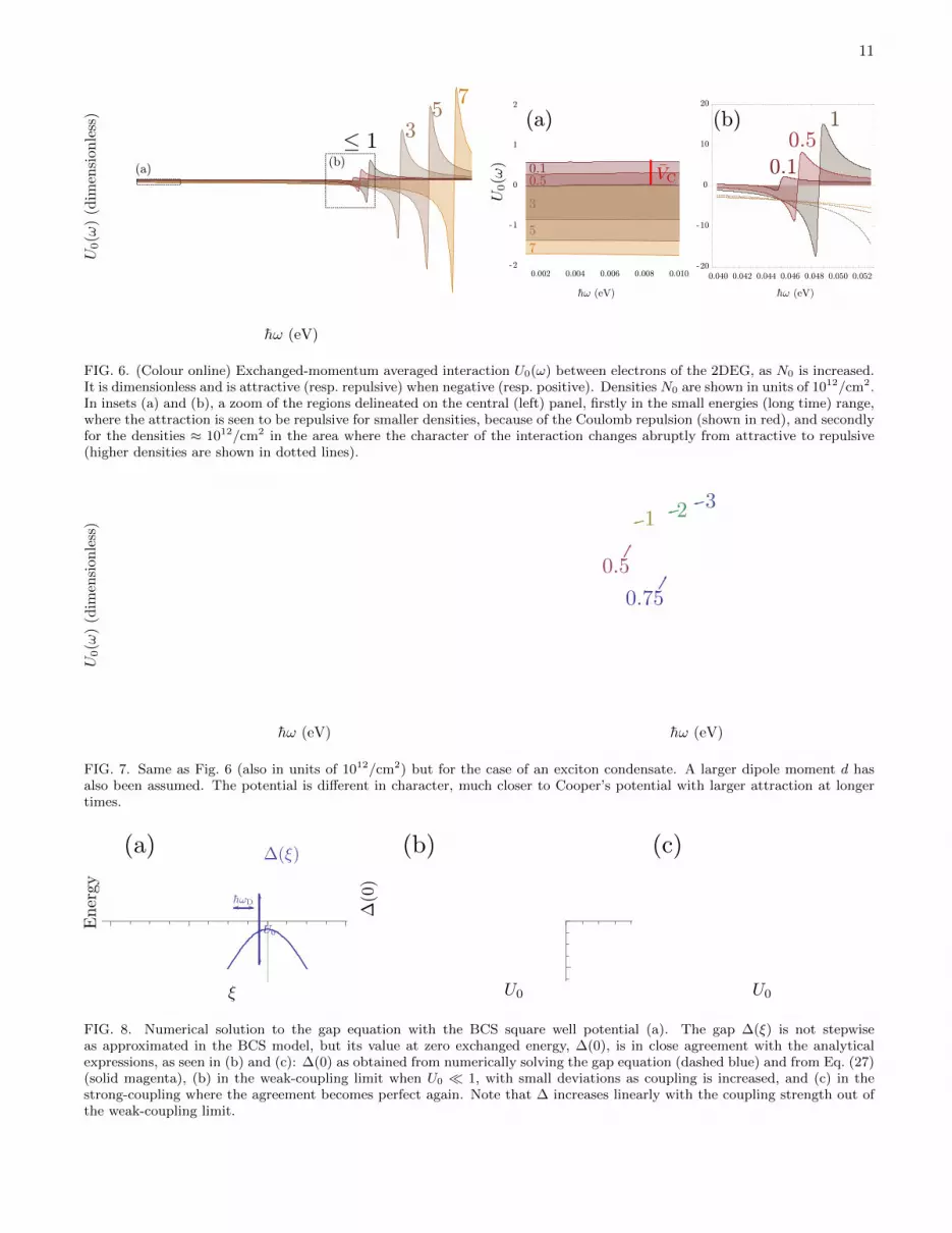
and assume all-excitonic interactions, X = 1, we can consider the same effect in the absence of a microcavity, relyingon a purely excitonic (rather than polaritonic) BEC. In this case, the same procedure as detailed above leads to aneffective potential as shown in Fig. 7. We kept all parameters the same for comparison except for the dipole moment,which we have taken three times as large (d = 12nm). This corresponds to the spatial separation of electrons andholes in the system of indirect excitons studied by Butov et al [38]. The potential we obtain in the exciton case isvery different in character from the polariton case, and is more closely related to the Cooper (conventional) shape ofa square well, or the Bogoliubov potential including repulsive elbows.

From these potentials, one can proceed to solve the gap equation.

11

0.040 0.042 0.044 0.046 0.048 0.050 0.052

-20

-10

0

10

20

0.002 0.004 0.006 0.008 0.010-2

-1

0

1

2

(a)

(a)

(b)

(b)7

53

10.5

0.1

7

5

3

0.50.1

FIG. 6. (Colour online) Exchanged-momentum averaged interaction U0(ω) between electrons of the 2DEG, as N0 is increased.It is dimensionless and is attractive (resp. repulsive) when negative (resp. positive). Densities N0 are shown in units of 1012/cm2.In insets (a) and (b), a zoom of the regions delineated on the central (left) panel, firstly in the small energies (long time) range,where the attraction is seen to be repulsive for smaller densities, because of the Coulomb repulsion (shown in red), and secondlyfor the densities ≈ 1012/cm2 in the area where the character of the interaction changes abruptly from attractive to repulsive(higher densities are shown in dotted lines).

3

0.75

0.5

1 2

FIG. 7. Same as Fig. 6 (also in units of 1012/cm2) but for the case of an exciton condensate. A larger dipole moment d hasalso been assumed. The potential is different in character, much closer to Cooper’s potential with larger attraction at longertimes.

(b) (c)(a)

FIG. 8. Numerical solution to the gap equation with the BCS square well potential (a). The gap ∆(ξ) is not stepwiseas approximated in the BCS model, but its value at zero exchanged energy, ∆(0), is in close agreement with the analyticalexpressions, as seen in (b) and (c): ∆(0) as obtained from numerically solving the gap equation (dashed blue) and from Eq. (27)(solid magenta), (b) in the weak-coupling limit when U0 � 1, with small deviations as coupling is increased, and (c) in thestrong-coupling where the agreement becomes perfect again. Note that ∆ increases linearly with the coupling strength out ofthe weak-coupling limit.

12

IV. GAP EQUATION

A. Cooper potential

The BCS gap equation (2) is easier to tackle as a continuous equation:

∆(ξ, T ) = −∫ ∞−∞

U0(ξ − ξ′)∆(ξ′, T ) tanh(E/2kBT )

2Edξ′ , (25)

where we have also introduced a finite temperature T from the Fermi-Dirac distribution of elementary excitations [50].With the BCS approximation of a step potential, the gap equation at zero temperature simplifies to ∆(ξ, T ) =

−U0

∫ ξ+~ωD

ξ−~ωD∆(ξ′, T )/2E dξ′. If ∆� ~ωD, the ξ dependence in the integral boundaries can be neglected (or, coming

back to Eq. (2), one sees that in the initial gap equation, ∆k is exactly constant if Ukk′ = U0 and is zero otherwise).Thus, we can assume the gap to be of the form:

∆(ξ) =

{∆(0) if |ξ| ≤ ~ωD ,

0 otherwise .(26)

In this case, simplifying ∆(0) on both side of Eq. (25), we obtain:

∆(0) = −~ωD/ sinh(−1/U0) . (27)

Equation (27) is better known as its approximation when U0 � 1, in which case it takes the form of the famousBCS gap expression, ∆(0) = 2~ωD exp(−1/U0).

Solving exactly the gap equation calls for some numerical method. Equation (25) is a nonlinear integral equation,of the type studied by Hammerstein, i.e.,

∆(ξ, T ) =

∫K(ξ, ξ′)f [ξ′,∆(ξ′)] dξ′ (28)

where in our case K(x, y) = −U0(x− y)/2 and f [y, z] = z tanh(√y2 + z2)

/√y2 + z2. There are strong conditions of

existence of nontrivial (nonzero) solutions when U0 ≤ 0 [51, 52], however the case when the kernel K is not positivedefinite, that is, in presence of repulsion,2 has been much less studied mathematically [53]. Cooper’s potential,being always negative, falls in the category of potentials which admit a unique nontrivial solution, with a stablenumerical technique to obtain it, namely, since the mapping is contractive, by iterations of the gap equation: aninitial (nonzero) function ∆0 is used to compute the rhs of Eq. (25), providing ∆1 which is injected back until thefunction converges. The gap computed in this way for a given Cooper potential is shown in Fig. 8(a). As one cansee, the BCS approximation (26) remains a rather coarse approximation, since the gap turns out in this case tobe bell-shaped rather than being a step function. Surprisingly, ∆(0) is however in much closer agreement with itsapproximation, as shown on Fig. 8(b) and (c) in the weak and strong coupling regime, respectively. There are smallquantitative deviations in (b) between the numerical points and the formula when using the exact parameters of thepotential. By fitting the numerical results, a perfect agreement can be found for slight variations of ~ωD and U0. TheBCS approximation therefore turns out to be an exceedingly good one as compared to an exact solution of the gapequation. For the procedure to make sense, similar results should be obtained for a smoothed well that approximatesthe BCS square well [41]. We will not address this point here, but go directly to the case where the potential is notalways attractive.

B. Bogoliubov potential

The potential is not always attractive when, for instance, some overall repulsion, such as direct Coulomb interaction,is superimposed on the attractive Cooper potential, as shown on Fig. 9. The Coulomb interaction is time independentand should therefore extend to all ω but here also a cutoff ωC is introduced to avoid divergencies. This results inan attractive, Cooper-like potential, flanked by two repulsive windows. Such a potential is known as the Bogoliubovpotential [54, 55].

2 as well as attraction, since the case of only repulsion admits only ∆ = 0 as a solution.

13

FIG. 9. Adding an overall repulsive Coulomb repulsion VC (red, left) until a cutoff ωC to the BCS potential V0 (green, left)results in the Bogoliubov stepwise potential (right). We take the convention V0, VC, U0 positive in the above representationand U0 = V0 − VC, so that, e.g., VC < 0 means attractive contribution of the “Coulomb repulsion”.

This approximation has been used to show extremely counter-intuitive behaviour of the gap equation and justifya-posteriori another heavily criticized approximation of BCS, neglecting Coulomb repulsion: the BCS mechanismindeed assumes only attraction between electrons, which can be dimmed by Coulomb repulsion, but which neverexplicitly appears as such (like in the Bogoliubov scenario). The great result of Cooper was that binding occurs atarbitrarily small attraction. An important result of the Bogoliubov potential is to show that the detrimental effectsof Coulomb repulsion are greatly reduced in the gap [55].

We now present a linearization of the gap equation that allows one to obtain an approximate solution for the criticaltemperature [54]. By assuming the gap equation to be a two step valued function ∆ = (∆1,∆2)T , the gap equationbecomes (I − 1)∆ = 0 with

I = −(−U0I1 VCI2

VCI1 VCI2

), (29)

where

I1 =

∫ ~ωD

−~ωD

tanh(ξ/(2kBTC))√ξ2 + ∆2

1

dξ ,≈ ln

(1.13~ωD

kBTC

), (30a)

I2 =

∫ ~ωC

~ωD

tanh(ξ/(2kBTC))√ξ2 + ∆2

2

dξ ≈ ln

(ωC

ωD

), (30b)

appear invariably in the columns of I. In Eq. (30a), the BCS approximation has been applied while in Eq. (30b),the fact that |ξ| � 0 has been used to neglect ∆ in the denominator and the temperature in the numerator. Theparametrization of the matrix in terms of the potential depends on the particular configuration (for example the relativewidths of the various layers of the structure). Here we have adopted the original parametrization of Bogoliubov, whichassumes narrow repulsive elbows surrounding a large attractive central region. Solving the linear equation for I1 andthen for the critical temperature, we find:

kBTC ≈ 1.13~ωD exp

− 1

V0 −VC

1 + I2VC

. (31)

In this form, one can see how Coulomb repulsion indeed introduces a small correction to the original BCS formula.The expression also seems to indicate that U0 could be repulsive (V0 − VC < 0) and still lead to a gap as long as thedenominator in Eq. (31) remains positive.

In the following, we compare these predictions with numerical solutions of the gap equation, keeping in mind thatthe iterative procedure is not assured, mathematically, to converge. We have observed that indeed, it sometimesencounters problems and exhibit strong instabilities, with bifurcations of solutions, for example.

In Fig. 10, we show the evolution of the gap function as VC is increased, from zero (BCS) to a point where theoverall potential is essentially repulsive. With onset of the repulsion, the gap acquires two negative sides and becomesa highly distorted function for large VC. Note that the approximation of constant gap over the various regions is atleast as good as for the case of BCS.

In Fig. 11, we now show the case where U0 = V0 − VC is held constant as the strength of the repulsion is variedindependently. In foresight of what is to come later, we also allow the elbows to be negative, that is, to contribute

14

0 2 4-2-4

(a) (b) (c) (d)Energy

0 2 4-2-4 0 2 4-2-4 0 2 4-2-4

0.4

0.2

0.0-0.2-0.4

FIG. 10. Gap (thick magenta and, magnified, thick khaki) of the Bogoliubov potential (filled blue) solved numerically for theparameters: ~ωD = 1, ~ωC = 2, V0 = 1 and VC taking values from (a) to (d) of: 0 (BCS), 0.1, 0.3 and 0.495. Coulomb repulsionresults in a dip in the gap function that, for increasing values, results in oscillations in the gap function. Paradoxically, evenwhen it is large and dominating attraction, repulsion does not prevent a gap, as seen in (d).

an additional attraction to the conventional mechanism (for now we do not consider physical justification of this).Another unexpected result is obtained: the repulsive potential is in this case favouring a larger gap, as can be seenby comparing (a), where the gap function is highly oscillatory, to (d) where it recovers the BCS bell-shape. In (h),the distorted but overall attractive potential still results in a BCS type gap, but wider and larger. Note how therepulsion, by “squeezing” the gap, allows it to achieve much higher values than for the case of smaller or no repulsion.

These unexpected results are confirmed phenomenologically by the Bogoliubov approximation Eq. (31), whichwe plot as a dashed line in Fig. 11, compared to ∆(0) computed numerically. Here we should emphasize that thetwo quantities are not meant to be compared quantitatively (as we did when comparing the BCS formula with thenumerical solution), since one, ∆(0) (computed numerically) is the gap at zero temperature while the other, kBTC isthe temperature at which the gap vanishes. There is a monotonous relationship between the two, that is, increasing∆(0) implies increasing TC, so one can appreciate the consistency of the results by observing similar trends. Theobstacle to conducting an extensive numerical comparison is that it is an intensive task numerically to compute TC,since this requires solution of the gap equation for various temperatures until the curve ∆(T ) is obtained and itsintersect with zero is found. A critical slowing down phenomenon makes the iterative process slower as the criticaltemperature is approached. In addition, numerical instabilities are stronger at nonzero T . Therefore, although itis relatively straightforward to compute ∆(0) numerically, it is not convenient to use this method to obtain TC.On the other hand, the Bogoliubov approximation gives a fair estimate of TC, but is not able to provide the gapat zero temperature, since at the core of its method, there is an assumption of vanishing ∆. Therefore, we havetwo complementary methods, each suited to provide a relevant aspect of the problem. We note that the gap atzero temperature is an important quantity which can be measured independently from TC by Andreev reflection inconductivity experiments, which is why we discuss it here in a great detail.

We can see, indeed, that the qualitative agreement is good and that the counter-intuitive features of the gapequation are reproduced by the analytical formula.

C. Polariton potential

In the case of the polariton problem, we have seen that, even when neglecting Coulomb repulsion (as in the originalBCS formulation), the potential U(ω) departs strongly from the Cooper potential and features two large attractiveregions far from small energies, immediately followed by two strong repulsive windows. We extend the Bogoliubovmethod to a three-step approximation of this potential, such as displayed in Fig. 13, with, in reference to previouspotentials, notations ωD, ωC and ωB for the boundaries of the central, shallow attractive region, narrow, deep attractiveregion and repulsive region, respectively. This is a notation only and is not mean to be understood as referring toDebye, Coulomb or Bogoliubov in any strict sense. Following the same premises, we approximate the gap equationby a three-step valued function ∆ = (∆1,∆2,∆3)T . This approximation turns out to be an exceedingly good one incertain cases, such as the one displayed in Fig. 13. Here there is even more room to choose a parametrization of theI matrix. We now give general guidelines on how to build this matrix. The simplest method is to fix ξ on the lhs ofEq. (25) at the center of each region and, in the corresponding row, take for each column the potential that is sampledmore by the difference |ξ − ξ′|. Refinements are possible, such as weighting elements of I by coefficients which reflecthow much time the variables ξ and ξ′ spend in the regions that determine the matrix equation. This problem hasthe following mathematical expression: how is the random variable X − Y distributed when X (resp. Y ) is uniformlydistributed in an interval [gi, gi+1] (resp. [hi, hi+1]). The solution is easily obtained as proportional (normalize to

15

4

2

0-2-4

4

2

0-2-4

0 2 4-2-4 0 2 4-2-4 0 2 4-2-4 0 2 4-2-4

(a) (b) (c) (d)

(e) (f) (g) (h)

Energy

Energy

FIG. 11. Gap (thick magenta and, magnified, thick khaki) of the Bogoliubov potential (filled blue) solved numerically for thefollowing parameters: ~ωD = 0.5, ~ωC = 2, V0−VC = 0.5 (fixed) and VC (the height of the elbow) taking values from (a) to (h)of: -5, -0.5, -0.1, 0 (BCS), 0.3, 0.5 (BCS), 1.5 and 5. The repulsive nature of the elbows change the character of the gap frombell-shaped to an oscillating function. The oscillating gap in the presence of strong repulsion allows, paradoxically, high valuesof the gap at zero-exchanged energy.

(a) (b) (c)

FIG. 12. ∆(0) for the case of Fig. 10 (a) and 11 (c), for their respective parameters, and (b), with ~ωD = .5, V0 = 1, ωC

changing as indicated and VC changing such that the area of the repulsive elbow is conserved.

unity) to:

P (X − Y = θ) ∝√

[max(gi, hi − θ)]−min(gi+1, hi+1 − θ)]2 + [max(θ + gi, hi)−min(θ + gi+1, hi+1]2 . (32)

This is easily obtained geometrically (the square root comes from Pythagoras’ theorem) and the problem results infinding the intersect of a line with the grid. There are two configurations. Working out the cases shows that Eq. (32)reduces to a triangular or a top-head truncated triangular distribution. The coefficients entering I can then be takenas the potentials weighted by the area intersecting their corresponding region. The soundness of such an approachcan be appreciated only if cases are checked numerically to compare quantitatively various parametrizations. Forsimplicity, we shall here consider cases where only the dominant potential is considered. An example of such a gapequation (I − 1)∆ = 0 is defined with:

I = −

V0I1 V1I2 −VCI3

V1I1 V0I2 V0I3

−VCI1 V0I2 V0I3

, (33)

where

Ii =

∫ ~ω>i

~ω<i

tanh(ξ/(2kBTC))√ξ2 + ∆2

i

dξ , (34)

and Ii is integrated on the respective steps, as defined by the integral boundary conditions, i.e., (ω<1 , ω>1 , ω

<2 , ω

>2 , ω

<3 , ω

>3 ) =

(0, ωD, ωD, ωC, ωC, ωB).

16

Energy

0.2

0.1

0.0

-0.1

-0.2

0 2 4-2-4

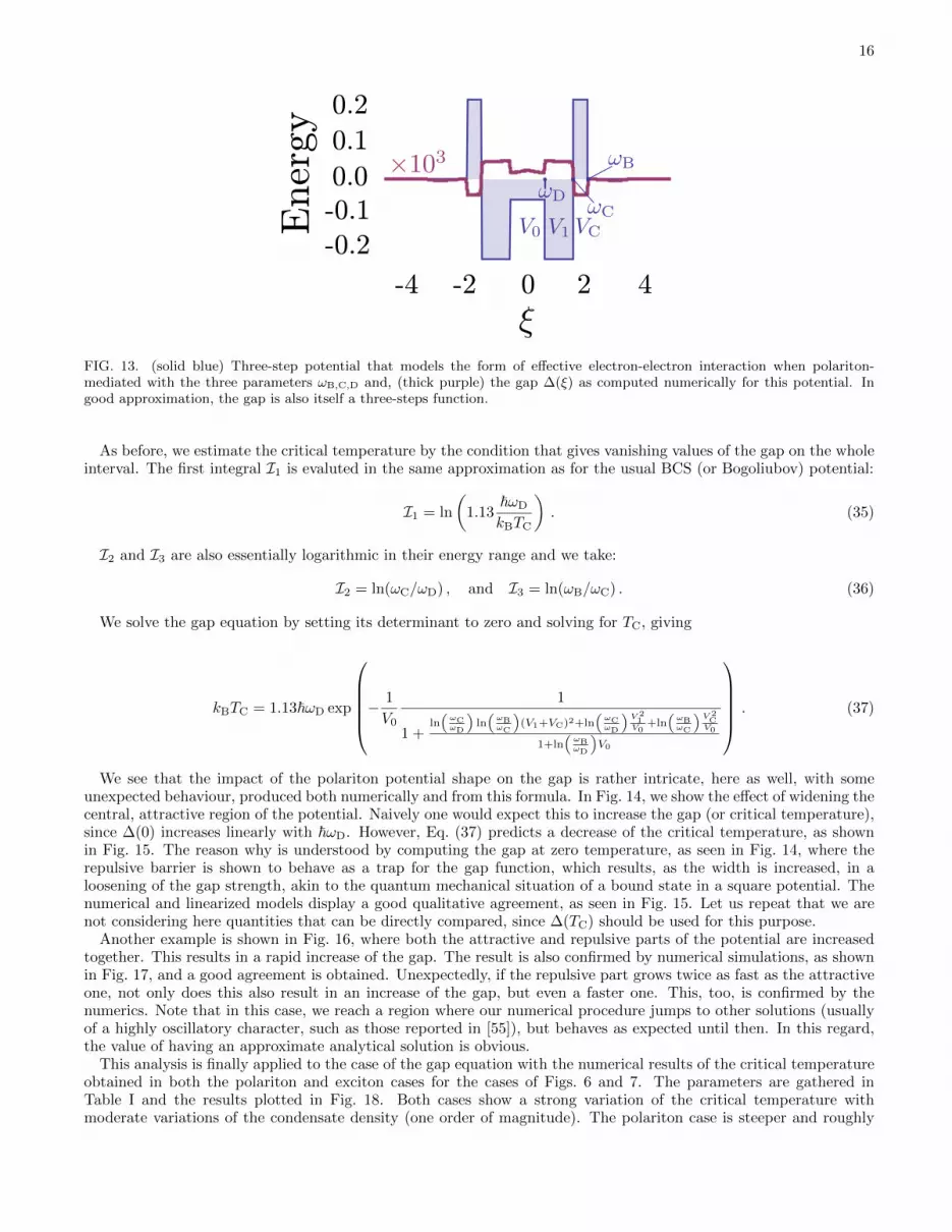
FIG. 13. (solid blue) Three-step potential that models the form of effective electron-electron interaction when polariton-mediated with the three parameters ωB,C,D and, (thick purple) the gap ∆(ξ) as computed numerically for this potential. Ingood approximation, the gap is also itself a three-steps function.

As before, we estimate the critical temperature by the condition that gives vanishing values of the gap on the wholeinterval. The first integral I1 is evaluted in the same approximation as for the usual BCS (or Bogoliubov) potential:

I1 = ln

(1.13

~ωD

kBTC

). (35)

I2 and I3 are also essentially logarithmic in their energy range and we take:

I2 = ln(ωC/ωD) , and I3 = ln(ωB/ωC) . (36)

We solve the gap equation by setting its determinant to zero and solving for TC, giving

kBTC = 1.13~ωD exp

− 1

V0

1

1 +ln(

ωCωD

)ln(

ωBωC

)(V1+VC)2+ln

(ωCωD

)V 21

V0+ln

(ωBωC

)V 2C

V0

1+ln(

ωBωD

)V0

. (37)

We see that the impact of the polariton potential shape on the gap is rather intricate, here as well, with someunexpected behaviour, produced both numerically and from this formula. In Fig. 14, we show the effect of widening thecentral, attractive region of the potential. Naively one would expect this to increase the gap (or critical temperature),since ∆(0) increases linearly with ~ωD. However, Eq. (37) predicts a decrease of the critical temperature, as shownin Fig. 15. The reason why is understood by computing the gap at zero temperature, as seen in Fig. 14, where therepulsive barrier is shown to behave as a trap for the gap function, which results, as the width is increased, in aloosening of the gap strength, akin to the quantum mechanical situation of a bound state in a square potential. Thenumerical and linearized models display a good qualitative agreement, as seen in Fig. 15. Let us repeat that we arenot considering here quantities that can be directly compared, since ∆(TC) should be used for this purpose.

Another example is shown in Fig. 16, where both the attractive and repulsive parts of the potential are increasedtogether. This results in a rapid increase of the gap. The result is also confirmed by numerical simulations, as shownin Fig. 17, and a good agreement is obtained. Unexpectedly, if the repulsive part grows twice as fast as the attractiveone, not only does this also result in an increase of the gap, but even a faster one. This, too, is confirmed by thenumerics. Note that in this case, we reach a region where our numerical procedure jumps to other solutions (usuallyof a highly oscillatory character, such as those reported in [55]), but behaves as expected until then. In this regard,the value of having an approximate analytical solution is obvious.

This analysis is finally applied to the case of the gap equation with the numerical results of the critical temperatureobtained in both the polariton and exciton cases for the cases of Figs. 6 and 7. The parameters are gathered inTable I and the results plotted in Fig. 18. Both cases show a strong variation of the critical temperature withmoderate variations of the condensate density (one order of magnitude). The polariton case is steeper and roughly

17

0 2 4-2-4

Energy

0.4

0.2

0.0

-0.2

-0.4

0 2 4-2-4 0 2 4-2-4 0 2 4-2-4

FIG. 14. Potential (filled blue) and its corresponding gap equation, solved numerically, as the size of the central attractiveplateau is increased. Somewhat unexpectedly, the gap decreases as a result. The repulsive barriers have the effect of squeezingthe gap up.

0.5 0.6 0.7 0.8 0.9 1. 1.1 1.2 1.3 1.4 1.50.000

0.005

0.010

0.015

0.020

0.025

0.030numericalmodel

FIG. 15. ∆(0) (joined points, blue) and kBTC from the three-step Bogoliubov approximation, in the case where the width ofthe central attraction is increased. Unexpectedly, this results in a decrease of the critical temperature.

linear while the exciton case increases less quickly but begins earlier. In both cases, temperatures are very high,and other effects will surely break the mechanism, for instance the loss of the condensate. This shows, however, therobustness of the mechanism in the conditions where it should apply.

V. CONCLUSIONS

We have studied possible mechanisms of superconductivity in semiconductor heterostructure systems where a Bose-Einstein condensate mediating the effective electron-electron interaction leads to enhancement of the coupling, yieldingvery high critical temperatures. We have considered the case of an exciton BEC, consisting of a sandwich of an n-doped QW containing the superconducting electrons, in contact with coupled QWs where the BEC of indirect excitonsis formed, for instance by optical excitation. We have also considered the case of a polariton BEC, where n-doped

(b) (c)

0 2 4-2-4 0 2 4-2-4 0 2 4-2-40 2 4-2-4

(a)

Energy

1.0

0.5

0.0

-0.5

-1.0

(d)

FIG. 16. Numerical solution of the gap equation when both the attractive and repulsive parts of the potential are increasedtogether (here in the same proportions), showing a rapid increase of the gap.

18

0.6 0.8 1.00.40.2

0.0

0.1

0.2

0.3

0.6 0.8 1.00.40.2

model numerics

0.0

0.1

0.2

0.3

FIG. 17. ∆(0) (joined points, blue) and kBTC from the three-step Bogoliubov approximation.

polaritons

excitons

room temperature

FIG. 18. (colour online) Critical temperature as a function of the condensate density N0 for the case of a polariton condensate(solid blue) and of an exciton condensate (dotted purple).

QWs and undoped QWs hosting excitons are embedded in a microcavity. We have computed in these two cases theeffective electron-electron interaction U(ω) as a function of the exchanged energy ~ω, showing how the retardationeffect acquires a peculiar character in the polariton case, namely, yielding a weakly attractive potential at longtimes, followed by a succession of strongly attractive and strongly repulsive windows. The gap equation in this caseexhibits strong differences as opposed to the case of the Cooper potential (of conventional BCS and exciton-BECmechanism). To understand the physical mechanism leading to large gaps and bypass numerical instabilities, westudied in detail the gap equation in the cases of simplified step-wise potentials, and offered an analytical methodto obtain the critical temperature, which is in qualitative agreement with the numerical results. Our results suggestrecord breaking critical temperatures in these systems. We stress, however, that the path towards achievement ofexciton mediated superconductivity at high temperatures may be long and full of obstacles. Of the two experimentallyrelevant systems that we have considered, one (coupled QWs) only shows the BEC of excitons at very low temperatures(less than 1K [38]). Consequently, one cannot expect high temperature superconductivity in this system, while at lowtemperatures the superconducting gap may be very large. In microcavities, polariton BEC or polariton lasing haveindeed been demonstrated at room temperature [17, 18]. However, embedding a high-quality n-doped QW insidethe cavity, the proper choice of the experimental geometry in order to minimise optical absorption in the dopedQW, and especially fabrication of quantum contacts for selective injection of carriers in the QW of interest, maypose technological difficulties. It is possible that hybrid metal-semiconductor or semi-metal semiconductor systemsmay appear more suitable for the observation of the predicted effects. A conventional superconductor put in contactwith a semiconductor also seems promising. Collective quantum phenomena in Bose-Fermi mixtures are extremelycomplicated and we foresee breakthroughs in their study in multilayer structures combining a Fermi gas of electronsand an exciton BEC.

19

ACKNOWLEDGMENTS

We are grateful to H. Ouerdanne and P. Lagoudakis for useful discussions. Support from EPSRC and EU FP7 ITNproject CLERMONT4 are acknowledged. I.A.S. thanks the support from Rannis “Center of excellence in polaritonics”and FP7 IRSES POLAPHEN project.

[1] A. Kavokin, J. J. Baumberg, G. Malpuech, and F. P. Laussy, Microcavities (Oxford University Press, 2007).[2] H. Deng, H. Haug, and Y. Yamamoto, Rev. Mod. Phys. 82, 1489 (2010).

[3] A. Imamoglu, R. J. Ram, S. Pau, and Y. Yamamoto, Phys. Rev. A 53, 4250 (1996).[4] J. J. Baumberg, P. G. Savvidis, R. M. Stevenson, A. I. Tartakovskii, M. S. Skolnick, D. M. Whittaker, and J. S. Roberts,

Phys. Rev. B 62, R16247 (2000).[5] M. S. Skolnick, T. A. Fisher, and D. M. Whittaker, Semicond. Sci. Technol. 13, 645 (1998).[6] P. G. Savvidis, J. J. Baumberg, R. M. Stevenson, M. S. Skolnick, D. M. Whittaker, and J. S. Roberts, Phys. Rev. Lett.

84, 1547 (2000).[7] R. M. Stevenson, V. N. Astratov, M. S. Skolnick, D. M. Whittaker, M. Emam-Ismail, A. I. Tartakovskii, P. G. Savvidis,

J. J. Baumberg, and J. S. Roberts, Phys. Rev. Lett. 85, 3680 (2000).[8] C. Ciuti, P. Schwendimann, and A. Quattropani, Phys. Rev. B 63, 041303 (2001).[9] C. Ciuti and I. Carusotto, Phys. Stat. Sol. B 242, 2224 (2005).

[10] I. A. Shelykh, Y. G. Rubo, G. Malpuech, D. D. Solnyshkov, and A. Kavokin, Phys. Rev. Lett. 97, 066402 (2006).[11] A. Kavokin, G. Malpuech, and F. P. Laussy, Phys. Lett. A 306, 187 (2003).[12] F. P. Laussy, G. Malpuech, A. Kavokin, and P. Bigenwald, Phys. Rev. Lett. 93, 016402 (2004).[13] M. H. Szymanska, J. Keeling, and P. B. Littlewood, Phys. Rev. Lett. 96, 230602 (2006).[14] J. Kasprzak, M. Richard, S. Kundermann, A. Baas, P. Jeambrun, J. M. J. Keeling, F. M. Marchetti, M. H. Szymanska,

R. Andre, J. L. Staehli, V. Savona, P. B. Littlewood, B. Deveaud, and Le Si Dang, Nature 443, 409 (2006).[15] R. Balili, V. Hartwell, D. Snoke, L. Pfeiffer, and K. West, Science 316, 1007 (2007).[16] E. del Valle, D. Sanvitto, A. Amo, F. P. Laussy, R. Andre, C. Tejedor, and L. Vina, Phys. Rev. Lett. 103, 096404 (2009).[17] S. Christopoulos, G. B. H. von Hogersthal, A. J. D. Grundy, P. G. Lagoudakis, A. V. Kavokin, J. J. Baumberg, G. Christ-

mann, R. Butte, E. Feltin, J.-F. Carlin, and N. Grandjean, Phys. Rev. Lett. 98, 126405 (2007).[18] J. J. Baumberg, A. V. Kavokin, S. Christopoulos, A. J. D. Grundy, R. Butte, G. Christmann, D. D. Solnyshkov,

G. Malpuech, G. B. H. von Hogersthal, E. Feltin, J.-F. Carlin, and N. Grandjean, Phys. Rev. Lett. 101, 136409 (2008).[19] A. Amo, D. Sanvitto, F. P. Laussy, D. Ballarini, E. del Valle, M. D. Martin, A. Lemaıtre, J. Bloch, D. N. Krizhanovskii,

M. S. Skolnick, C. Tejedor, and L. Vina, Nature 457, 291 (2009).[20] D. Sanvitto, A. Amo, F. P. Laussy, A. Lemaıtre, J. Bloch, C. Tejedor, and L. Vina, Nanotechnology 21, 134025 (2010).[21] A. Amo, J. Lefrere, S. Pigeon, C. Adrados, C. Ciuti, I. Carusotto, R. Houdre, E. Giacobino, and A. Bramati, Nat. Phys.

5, 805 (2009).[22] K. G. Lagoudakis, M. Wouters, M. Richard, A. Baas, I. Carusotto, R. Andre, L. S. Dang, and B. Deveaud-Pledran, Nat.

Phys. 4, 706 (2008).[23] K. G. Lagoudakis, T. Ostatnicky, A. V. Kavokin, Y. G. Rubo, R. Andre, and B. Deveaud-Pledran, Science 326, 974

(2009).[24] D. Sanvitto, F. M. Marchetti, M. H. Szymanska, G. Tosi, M. Baudisch, F. P. Laussy, D. N. Krizhanovskii, M. S. Skolnick,

L. Marrucci, A. Lemaıtre, J. Bloch, C. Tejedor, and L. Vina, Nat. Phys. 6, 527 (2010).[25] A. Kavokin, D. Solnyshkov, and G. Malpuech, J. Phys.: Condens. Matter 19, 295212 (2007).[26] F. P. Laussy, A. V. Kavokin, and I. A. Shelykh, Phys. Rev. Lett. 104, 106402 (2010).[27] L. N. Cooper, Phys. Rev. 104, 1189 (1956).[28] J. Bardeen and D. Pines, Phys. Rev. 99, 1140 (1955).[29] J. Bardeen, Rev. Mod. Phys. 23, 261 (1951).[30] A. J. Leggett, Quantum Liquids (Oxford University Press, 2006).[31] J. Bardeen, L. N. Cooper, and J. R. Schrieffer, Phys. Rev. 106, 162 (1957).[32] J. Bardeen, L. N. Cooper, and J. R. Schrieffer, Phys. Rev. 108, 1175 (1957).[33] D. Allender, J. Bray, and J. Bardeen, Phys. Rev. B 7, 1020 (1973).[34] W. A. Little, Phys. Rev. 134, A1416 (1964).[35] V. L. Ginzburg, Sov. Phys.-Usp. 13, 335 (1970).[36] J. G. Bednorz and K. A. Muller, Z. Phys. B 64, 189 (1986).[37] A. J. Leggett, Nat. Phys. 2, 134 (2006).[38] L. V. Butov, C. W. Lai, A. L. Ivanov, A. C. Gossard, and D. S. Chemla, Nature 417, 47 (2002).[39] L. V. Butov, L. S. Levitov, A. V. Mintsev, B. D. Simons, A. C. Gossard, and D. S. Chemla, Phys. Rev. Lett. 92, 117404

(2004).[40] R. Rapaport, G. Chen, D. Snoke, S. H. Simon, L. Pfeiffer, K. West, Y. Liu, and S. Denev, Phys. Rev. Lett. 92, 117405

(2004).

20

[41] V. Ginzburg and D. Kirzhnits, eds., High-Temperature Superconductivity (Springer, 1982).[42] P. Monthoux, D. Pines, and G. G. Lonzarich, Nature 450, 1177 (2007).[43] R. Butte and N. Grandjean, Semicond. Sci. Technol. 26, 014030 (2010).[44] F. Tassone and Y. Yamamoto, Phys. Rev. B 59, 10830 (1999).[45] M. J. Bijlsma, B. A. Heringa, and H. T. C. Stoof, Phys. Rev. A 61, 053601 (2000).[46] V. L. Ginzburg, On Superconductivity and Superfluidity (Springer, 2009).[47] I. A. Shelykh, T. Taylor, and A. V. Kavokin, Phys. Rev. Lett. 105, 140402 (2010).[48] W. J. Thompson, Computers in Physics 12, 94 (1998).[49] J. V. Noble, Computing in Science and Engineering 2, 92 (2000).[50] P. G. de Gennes, Superconductivity Of Metals And Alloys (Westview Press, 1999).[51] M. Kitamura, Prog. of Th. Phys. 30, 435 (1963).[52] A. Vansevenant, Physica D 17, 339 (1985).[53] P. P. Zabreiko and A. I. Povolotskii, Ukrainian Mathematical Journal 22, 150 (1967).[54] J. B. Ketterson and S. N. Song, Superconductivity (Cambridge University Press, 1999).[55] X. H. Zheng and D. G. Walmsley, Phys. Rev. B 71, 134512 (2005).