arX

iv:m

ath/

0405

151v

1 [

mat

h.G

T]

9 M

ay 2

004

Symmetry is a vast subject, significant in art and nature.Mathematics lies at its roots, and it would be hard to finda better one on which to demonstrate the working of themathematical intellect. [Hermann Weyl, Symmetry [We]]

Symmetric knots and billiard knots.

by Jozef H.Przytycki

Symmetry of geometrical figures is reflected in regularities of theiralgebraic invariants. Algebraic regularities are often preserved whenthe geometrical figure is topologically deformed. The most natural,intuitively simple but mathematically complicated, topological objectsare knots.

We present in this papers several examples, both old and new, ofregularity of algebraic invariants of knots. Our main invariants are theJones polynomial (1984) and its generalizations.

In the first section, we discuss the concept of a symmetric knot, andgive one important example – a torus knot. In the second section, wegive review of the Jones type invariants. In the third section, we gentlyand precisely develop the periodicity criteria from the Kauffman bracket(ingenious version of the Jones polynomial). In the fourth section, we ex-tend the criteria to skein (Homflypt) and Kauffman polynomials. In thefifth section we describe rq periodicity criteria using Vassiliev-Gusarovinvariants. We also show how the skein method may be used for rq pe-riodicity criteria for the classical (1928) Alexander polynomial. In thesixth section, we introduce the notion of Lissajous and billiard knotsand show how symmetry principles can be applied to these geometricknots. Finally, in the seventh section, we show how symmetry can beused to gain nontrivial information about knots in other 3-manifolds,and how symmetry of 3-manifolds is reflected in manifold invariants.

1

1 Symmetric knots.

We analyze, in this paper, symmetric knots and links, that is, linkswhich are invariant under a finite group action on S3 or, more generally,a 3-manifold.

For example, a torus link of type (p, q) (we call it Tp,q) is preservedby an action of a group Zp ⊕ Zq on S3 (c.f. Fig. 1.1 and Example 1.1).

Fig. 1.1. The torus link of type (3, 6), T3,6

Example 1.1 Let S3 = z1, z2 ∈ C ×C : |z1|2 + |z2|2 = 1. Let us con-sider an action of Zp⊕Zq on S3 which is generated by Tp and Tq, whereTp(z1, z2) = (e2πi/pz1, z2) and Tq(z1, z2) = (z1, e

2πi/qz2). Show that thisaction preserves torus link of type (p, q). This link can be described as

the following set (z1, z2) ∈ S3 : z1 = e2πi( t

p+ k

p), z2 = e2πit/q, where t

is an arbitrary real number and k is an arbitrary integer.If p is co-prime to q then Tp,q is a knot and can be parameterized by:

R ∋ t 7→ (e2πit/p, e2πit/q) ∈ S3 ⊂ C2.

In this case Zp ⊕ Zq = Zpq with a generator T = TpTq.

Subsequently, we will focus on the action of a cyclic group Zn. Wewill mainly consider the case of an action on S3 with a circle of fixedpoints. The new link invariants, (see Section 2), provide efficient criteriafor examining such actions.

Definition 1.2 A link is called n-periodic if there exists an action of Zn

on S3 which preserves the link1 and the set of fixed points of the action

1More precisely we require an existence of an embedding of circles, realizing thelink, which is equivariant under the group action.

2

is a circle disjoint from the link. If, moreover, the link is oriented thenwe assume that a generator of Zn preserves the orientation of the linkor changes it globally (that is on every component).

2 Polynomial invariants of links

We will describe in this section polynomial invariants of links, crucialin periodicity criteria. We start from the skein (Jones-Conway or Hom-flypt) polynomial, PL(v, z) ∈ Z[v±1, z±1] (i.e. PL(v, z) is a Laurentpolynomial in variables v and z).

Definition 2.1 The skein polynomial invariant of oriented links in S3

can be characterized by the recursive relation (skein relation):

(i) v−1PL+(v, z)− vPL−(v, z) = zPL0(v, z), where L+, L− and L0 are

three oriented link diagrams, which are the same outside a smalldisk in which they look as in Fig. 2.1,

and the initial condition

(ii) PT1 = 1, where T1 denotes the trivial knot.

+L -L L 0

Fig. 2.1

We need some elementary properties of the skein polynomial:

Proposition 2.2 (a) ([L-M]) zcom(L)−1PL(v, z) ∈ Z[v±1, z] where com(L)is the number of link components of L. That is we do not use neg-ative powers of z. Furthermore the constant term, with respect tovariable z, is non-zero.

(b) PL(v, z)−PTcom(L)is divisible by (v−1 − v)2 − z2. Here Ti denotes

the trivial link of i components.

3

(c) Let PL(v, z) = zcom(L)−1PL(v, z), then PL(v, z)−(v−1−v)com(L)−1

is divisible by (v−1 − v)2 − z2

(d) PL(v, z) ≡ (v3z)jPTk(v, z) mod (v6−1

v2−1 , z2 + 1)for some j and k where j ≡ (k − com(L)) mod 2. In particular

PL ≡ δPL mod (v6−1v2−1 , z2 + 1) where δ equals to 1 or −1 and L

denotes the mirror image of L.

Proof:

(a)-(c) Initial conditions and recurrence relation give immediately thatPL(v, z) ∈ Z[v±1, z]. (c) holds for trivial links from the definition(the difference is zero). To make inductive step, first notice thatPL(v, z) satisfies the skein relation v−1PL+(v, z) − vPL−

(v, z) =

z2ǫPL0(v, z) where ǫ is equal to 0 in the case of the selfrossing ofL+ and ǫ = 1 in the mixed crossing case. We can rewrite the skeinrelation so that the inductive step is almost obvious:

v−1(PL+ − (v−1 − v)comL+−1) − v(PL−− (v−1 − v)comL−−1) =

z2ǫ(PL0 − (v−1 − v)comL0−1) + (v−1 − v)comL+−2ǫ(v−1 − v)2ǫ − z2ǫ)

Namely the last term in the equality is always divisible by (v−1 −v)2 − z2 therefore if two other are divisible then the last one is.We completed the proof of (c). From (c) follows that PL(1, 0) = 1,thus the second part of (a) follows. (b) is just a weaker version of(c).

(d) It can be derived from the relation of PL(e2sπi/6,±1) and the firsthomology group (modulo 3) of the 2-fold branched cyclic cover of(S3, L) [L-M, Yo-1, Ve].

2

Definition 2.3 Let L be an unoriented diagram of a link. Then theKauffman bracket polynomial 〈L〉 ∈ Z[A∓1] is defined by the followingproperties:

1. 〈©〉 = 1

4

2. 〈© ⊔ L〉 = −(A2 + A−2)〈L〉

3. 〈 〉 = A〈 〉 + A−1〈 〉

The Kauffman bracket polynomial is a variant of the Jones polyno-mial for oriented links. Namely, for A = t−

14 and D being an oriented

diagram of L we have

VL(t) = (−A3)−w(D) < D > (1)

where w(D) is the planar writhe (twist or Tait number) of D equal tothe algebraic sum of signs of crossings.

Kauffman noted that VL(t) = PL(t,√

t− 1√t). In particular t−1VL+−

tVL−= (

√t − 1√

t)VL0 . Proposition 2.2 gives us:

Corollary 2.4 (a) [Jo]. For a knot K, VK(t) ∈ Z[t±1] and VK(t)−1is divisible by (t − 1)(t3 − 1).

(b) [Yo-1]. For a knot K, VK(t)−δVK(t−1) is divisible by t3+1t+1 , where

δ equals to 1 or −1.

In the summer of 1985 (two weeks before discovering the “bracket”),L. Kauffman invented another invariant of links [Ka], FL(a, z) ∈ Z[a±1, z±1],generalizing the polynomial discovered at the beginning of 1985 byBrandt, Lickorish, Millett and Ho [B-L-M, Ho]. To define the Kauffmanpolynomial we first introduce the polynomial invariant of link diagramsΛD(a, z). It is defined recursively by:

(i) Λo(a, z) = 1,

(ii) Λ (a, z) = aΛ|(a, z); Λ (a, z) = a−1Λ|(a, z),

(iii) ΛD+(a, z) + ΛD−(a, z) = z(Λ0(a, z) + ΛD∞

(a, z)).

The Kauffman polynomial of oriented links is defined by

FL(a, z) = a−w(D)ΛD(a, z)

where D is any diagram of an oriented link L.

5

Remark 2.5 Let F ∗(a, z) be the Dubrovnik variant of the Kauffmanpolynomial 2. The polynomial F ∗ satisfies initial conditions F ∗

Tn=

(a−a−1

z + 1)n−1 and the recursive relation aw(D+)F ∗D+

− aw(D−)F ∗D−

=

z(aw(D0)F ∗D0

− aw(D∞)F ∗D∞

). Lickorish noted that the Dubrovnik poly-nomial is just a variant of the Kauffman polynomial:F ∗

L(a, z) = (−1)(com(L)−1)FL(ia,−iz), ([Li]).

Proof.We check the formula for trivial links and then show that if it holds forthree terms of the skein relation it also holds for the fourth one.

(i) FTn(ia,−iz) = (−1)(n−1)(a−a−1

−z − 1)n−1 = F ∗Tn

(a, z).

(ii) (ia)w(D+)FD+(ia,−iz)+(ia)w(D−)FD−(ia,−iz) = (−iz)((ia)w(D0)FD0+

(ia)w(D∞)FD∞). This reduces to aw(D+)F ∗

D+−aw(D−)F ∗

D−= z(aw(D0)F ∗

D0+

(−1)com(D0)−com(D∞)aw(D∞)F ∗D∞, which gives the skein relationfor F ∗

D(a, z).

3 Periodic links and the Jones polynomial.

Periodicity of links is reflected in the structure of new polynomials oflinks. We will describe this with details in the case of the Jones poly-nomial (and the Kauffman bracket), mostly following [Mu-2, T-1, P-3,Yo-1] but also proving new results. Let D be an r-periodic diagram of anunoriented r-periodic link, that is ϕ(D) = D where ϕ denote the rota-tion of R3 along the vertical axis by the angle 2π/r. In the coordinatesof R3 given by a complex number (for the first two real co-ordinates)and a real number (for the third) one gets: φ(z, t) = (e2πi/rz, t). ϕis a generator of the group Zr acting on R3 (and S3 = R3 ∪ ∞). Inparticular ϕr = Id. See Fig. 3.1.

2Kauffman described the polynomial F∗ on a postcard to Lickorish sent from

Dubrovnik in September ’85.

6

...

.

...

......

... ...

...

γ

ϕ

Fig. 3.1

By the positive solution to the Smith Conjecture [Sm, Thur], every r-periodic link has an r-periodic diagram, thus we can restrict ourselvesto considerations of these, easy to grasp, diagrams. With the help ofelementary group theory we have the following fundamental lemma.

Lemma 3.1 Let D be an unoriented r-periodic link diagram, r prime.Then the Kauffman bracket polynomial satisfies the following “periodic”formula:

Dsym( )

≡ ArDsym( )

+ A−rDsym( )

mod r

where Dsym( )

,Dsym( )

and Dsym( )

denote three ϕ-invariant dia-

grams of links which are the same outside of the Zr-orbit of a neighbor-hood of a fixed single crossing, c (i.e. c, ϕ(c),..., ϕr−1(c)) at which they

differ by replacing by or , respectively.

Proof: Let us build the binary computational resolving tree of D us-ing the Kauffman bracket skein relation for every crossing of the orbit

7

(under Zr action), c, ϕ(c),..., ϕr−1(c). The tree has therefore 2r leavesand a diagram at each leaf contributes some value (polynomial) to theKauffman bracket polynomial of D = D

sym( )

, see Fig. 3.2. The

idea of the proof is that only extreme leaves, Dsym( )

and Dsym( )

,

contribute to < D > mod r.

.

.. .

.

. . . .

....

...

c

(c)φφ(c)

φn-1

(c)φ

n-1(c)

( )( )sym sym

sym ( )D

D D

Fig. 3.2

We need now some, elementary, group theory:Let a finite group G acts on a set X, that is every element g ∈ G “moves”X (g : X → X) and hg(x) = h(g(x)) for any x ∈ X and h, g ∈ G. Fur-thermore we require that the identity element of G is not moving X(e(x) = x where e is the identity element of G). The orbit of an elementx0 in X is the set of all elements of X which can be obtained from x0 byacting on it by G (Ox0 = x ∈ X | there is g such that g(x0) = x).The standard, but important, fact of elementary group theory is thatthe number of elements in an orbit divides the order (number of ele-ments) of the group. In particular if the group is equal to Zr, r prime,then orbits of Zr action can have one element (such orbits are calledfixed points) or r elements.After this long group theory digression, we go back to our leaf diagramsof the binary computational resolving tree of D. We claim that Zr actson the leaf diagrams and the only fixed points of the action are extremeleaves D

sym( )and D

sym( ). All other orbits have r elements and

8

they would cancel their contribution to < D > modulo r. To see thesewe introduce an adequate notation: Let ci = ϕ(c) and D

c0,...,cr−1s0,...,sr−1, where

si = or , denote the diagram of a link obtained from D by smooth-ing the orbit of crossings, c0, ...cr−1 according to indices si. D

c0,...,cr−1s0,...,sr−1

are leaves of our binary computational resolving tree of D, and the Zr

action can be fully described by the action on the indices s0, ..., sr−1.Namely ϕ(s0, ...sr−2, sr−1) = (sr−1, s0, ..., sr−2). From this description

it is clear that the only fixed point sequences are ( , ..., , ) and

( , ..., , ) and that diagrams from the given orbit represent equiv-alent (ambient isotopic) links, they just differ by the rotation of R3.From this follows that the contribution to < D > of an r element orbitis equal to 0 modulo r. Thus all leaves, but the fixed points, do notcontribute to < D > modulo r. The contribution of the fixed pointleaves is expressed in the formula of Lemma 3.1. 2

Corollary 3.2 Let Do be an oriented r-periodic link diagram, r prime,and D the same diagram, orientation forgotten.

(i ) Then the Kauffman bracket polynomial satisfies the followingformula:

Ar < Dsym( )

> −A−r < Dsym( )

>≡

(A2r − A−2r) < Dsym( )

> mod (r)

(ii ) Let fDo(A) = (−A3)−w(Do) < D > then

−A4rfDosym(+)

+ A−4rfDosym(−)

≡ (A2r − A−2r)fDosym(0)

mod (r)

Here Dosym(+) = Do

sym( ))

, Dosym(−) = D

sym( )

and Dosym(0) =

Dsym( )

denote three ϕ-invariant oriented diagrams of links which

are the same outside of the Zr-orbit of a fixed single crossing and

which at a neighborhood of the crossing differ by replacing by

or ;

9

(iii )

t−rVDosym(+)

− trVDosym(−)

≡ (tr/2 − t−r/2)VDosym(0)

mod (r)

Proof:

(i ) Use Lemma 3.1 for Dsym( )

and Dsym( )

and reduce the

term Dsym( )

.

(ii ) (i) can be written as:

(−A3)w(Do

sym(+))ArfDo

sym(+)−(−A3)

w(Dosym(−)

)A−rfDo

sym(−)≡ (A2r−

A−2r)(−A3)w(Do

sym(0))fDo

sym(0)mod (r) and using the equality w(Do

sym(+)) =

w(Dosym(−)) + 2r = w(Do

sym(0)) + r, one gets the congruence (ii).

(iii) This follows from (ii) by putting VL(t) = fL(A), for t = A−4.

2

Lemma 3.1 and Corollary 3.2 have several nice applications:to symmetric knots, periodic 3-manifolds and to analysis of connectionsbetween skein modules of the base and covering space in a covering (seeSection 7). Below are two elementary but illustrative applications toperiodic links.

Theorem 3.3 ([T-1, P-3]) (i) If L is an r-periodic oriented link (ris a prime), then its Jones polynomial satisfies the relation

VL(t) ≡ VL(t−1) mod (r, tr − 1).

(ii) Let us consider a polynomial VL(t) = (t12 )−3lk(L)VL(t) which is an

invariant of an ambient isotopy of unoriented links. lk(L) denoteshere the global linking number of L, any orientation of L gives thesame VL(t).If L is an r-periodic unoriented link (r is an odd prime), thenVL(t) ≡ VL(t−1) mod(r, tr − 1).

10

Theorem 3.4 Let K be an r-periodic knot with linking number k withthe fixed point set axis. Then

tr(k−1)/2VK(t) ≡ (t(k+1)/2 − t(−k−1)/2) − (t(k−1)/2 − t(1−k)/2)

t − t−1mod (r, tr−1).

In particular:

(a) If k is odd then VK(t) ≡ tk/2+t−k/2

t1/2+t−1/2 ≡ t(k−1)/2 − t(k−3)/2 + ... −t(3−k)/2 + t(1−k)/2 mod (r, tr − 1),

(b) If k is even then tr/2VK(t) ≡ tk/2+t−k/2−2(−1)k/2

t1/2+t−1/2 +(−1)k/2 tr+1t1/2+t−1/2 mod (r, tr−

1).

Proof:

3.3(i) From Corollary 3.2(iii) follows that VDosym(+)

≡ VDosym(−)

mod (r, tr−1). On the other hand we can change Do to its mirror image Do

by a sequence of changes of type Dosym(+) ↔ Do

sym(−). Therefore

VDo(t) ≡ VDo(t) mod (r, tr − 1). Theorem 3.3(i) follows becauseVDo(t) = VDo(t−1).

3.3(ii) The link L may be oriented so that ϕ (a generator of the Zr

action) preserves the orientation of L (first we orient L∗ = L/Zr

the quotient of L under the group action and then we lift theorientation up to L). For such an oriented L we get from (i):

VL(t) ≡ VL(t−1) mod (r, tr − 1)

and thus

(t12 )3lkLVL(t) ≡ (t

12 )−3lkLVL(t−1) mod (r, tr − 1)

and consequently

VL(t) ≡ t−3lk(L)VL(t−1) mod (r, tr − 1).

For r > 2, lk(L) ≡ 0 mod r so Theorem 3.3(ii) follows.

11

3.4 We proceed as in the proof of 3.3(i) except that instead of aimingat mirror image we aim the appropriate torus knot. To see thisit is convenient to think of our link L being in a solid torus andsimplify its quotient L∗ = L/Zn in the solid torus (see Section 7).The formula for the Jones polynomial of the torus knot, T(r,k), wasfound by Jones [Jo]:

VT(r,k)(t) = tr(k−1)/2 t(k+1)/2 − t(−k−1)/2 − tr(t(k−1)/2 − t(1−k)/2

t − t−1.

In Section 7, we discuss elementary proof of the formula and give ashort proof of the generalization of the Jones formula to the solidtorus (modulo r) using Lemma 3.1.

2

Theorem 3.3 is strong enough to allow Traczyk [T-1] to completeperiodicity tables for knots up to 10 crossings (for r > 3), that is, todecide whether the knot 10101 is 7-periodic.

Example 3.5 The knot 10101 (Fig.3.3) is not r-periodic for r ≥ 5.

10 101

Fig. 3.3

The Jones polynomial for 10101 is equal to

V10101(t) = t2−3t3+7t4−10t5+14t6−14t7+13t8−11t9+7t10−4t11+t12.

Thus, for r ≥ 5 it follows that V10101(t) 6≡ V10101(t−1 mod (r, tr − 1). In

particular, it follows that V10101(t) ≡ t−1 + 2 + 3t3 mod (5, t5 − 1) andalso V10101(t) ≡ 3t−3 + 5t−2 + 6t + 4t2 + 4t3 mod (7, t7 − 1).

12

Remark 3.6 Theorem 3.3 and 3.4 do not work for knots and r = 3. Itis the case because by Corollary 2.4, for any knot, VK(t) ≡ 1 mod (t3 −1). One should add that the classical Murasugi criterion using theAlexander polynomial, Theorem 5.3 ([Mu-1]) is working for r = 3, andTraczyk developed the method employing the skein polynomial, Theorem4.10(a) ([T-2, T-3]).

Yokota proved in [Yo-1] the following criterion for periodic knotswhich generalize Theorem 3.3 and is independent of Theorem 3.4.

Theorem 3.7 Let K be an r-periodic knot (r is an odd prime) withlinking number k with the fixed point set axis. Then

(a) If k is odd then VK(t) ≡ VK(t−1) mod (r, t2r − 1),

(b) If k is even then VK(t) ≡ trVK(t−1) mod (r, t2r−1t+1 ).

We can extend Theorems 3.3, 3.4 and 3.7 (or rather show its limits)by considering the following operations on link diagrams:

Definition 3.8 (i) A tk move is an elementary operation on an ori-ented link diagram L resulting in the diagram tk(L) as shown onFig. 3.4.

k positive half twistst movek

L t (L)k...

Fig. 3.4

(ii) A tk move, k even, is an elementary operation on an oriented linkdiagram L resulting in the diagram tk(L) as shown on Fig. 3.5.

t movekL ... t (L)k

k half twists (k even)

Fig. 3.5

(iii) The local change in a link diagram which replaces parallel lines byk positive half-twists is called a k-move; see Fig.3.6.

13

k-move...

k right handed half twists

Fig. 3.6

Lemma 3.9 Let Lk be an unoriented link obtained from L0 by a k

move. Then < Lk >= Ak < L0 > +A−3k+2 A4k−(−1)k

A4+1 .

Proof: It follows by an induction on k. 2

Corollary 3.10 If L and L′ are oriented t2r, t2r equivalent links (thatis L and L′ differ by a sequence of t2r, t2r-moves) then

VL(t) ≡ trjVL′(t) mod (r, t2r−1t+1 ), for some integer j.

Proof: For k = 2r we have from Lemma 3.9 < L2r >= A2r < L0 >+A−6r+2(A4r − 1)A4r+1

A4+1 < L∞ >. Thus < L2r >≡ A2r < L0 >

mod (A4r − 1)A4r+1A4+1 and Corollary 3.10 easily follows. 2

4 Periodic links and the generalized Jones poly-

nomials.

We show here how periodicity of links is reflected in regularities of skeinand Kauffman polynomials. We explore the same ideas which werefundamental in Section 3, especially we use variations of Lemma 3.1.

Let R be a subring of the ring Z[v∓1, z∓1] generated by v∓1, z andv−1−v

z . Let us note that z is not invertible in R.

Lemma 4.1 For any link L its skein polynomial PL(v, z) is in the ringR.

Proof: For a trivial link Tn with n components we have PTn(v, z) =

(v−1−vz )n−1 ∈ R. Further, if PL+(v, z) (respectively PL−

(v, z)) andPL0(v, z) are in R then PL−

(v, z) (respectively PL+(v, z)) is in R aswell. This observation enables a standard induction to conclude 4.1.Now we can formulate our criterion for r-periodic links. It has an espe-cially simple form for a prime period (see Section 5 for a more generalstatement). 2

14

Theorem 4.2 Let L be an r-periodic oriented link and assume that ris a prime number. Then the skein polynomial PL(v, z) satisfies therelation

PL(v, z) ≡ PL(v−1,−z) mod (r, zr)

where (r, zr) is an ideal in R generated by r and zr.

In order to apply Theorem 4.2 effectively, we need the following fact.

Lemma 4.3 Suppose that w(v, z) ∈ R is written in the form w(v, z) =∑i ui(v)zi, where ui(v) ∈ Z[v∓1]. Then w(v, z) ∈ (r, zr) if and only if

for any i ≤ r the coefficient ui(v) is in the ideal (r, (v−1 − v)r−i).

Proof: ⇐ Suppose ui(v) ∈ (r, (v−1 − v)r−i) for i ≤ r. Now ui(v)zi ≡(v−1 − v)r−i)zip(v) ≡ (v−1−v

z )r−izrp(v) mod r, where p(v) ∈ Z[v±1].Thus ui(v)zi ∈ (r, zr) and finally w(v, z) ∈ (r, zr).⇒ Suppose that w(v, z) ∈ (r, zr), that is, w(v, z) ≡ zrw(v, z)mod r forsome w(v, z) ∈ R. The element w(v, z) can be uniquely written as a

sum w(v, z) = zu(v, z) +∑

j≥0(v−1−v

z )juj(v), where u(v, z) ∈ Z[v∓1, z]and uj(v) ∈ Z(v∓1). Thus, for i ≤ r (j = r − i) we have ui(v) ≡(v−1−v)r−iur−i(v) mod r and finally ui(v) ∈ (r, (v−1 −v)r−i) for i ≤ r.2

Example 4.4 Let us consider the knot 11388, in Perko’s notation [Per],see Fig.4.1. The skein polynomial P11388(v, z) is equal to

(3−5v−2+4v−4−v−6)+(4−10v−2+5v−4)z2+(1−6v−2+v−4)z4−v−2z6.

Let us consider the polynomial P11388(v, z) − P11388(v−1,−z). The coef-

ficient u0(v) for this polynomial is equal to 5(−v−2 +v2)+4(v−4−v4)−v−6+v6 and thus for r ≥ 7 we have u0(v) 6∈ (r, (v−1−v)r) = (r, v−r−vr).Now, from Lemma 4.3 we have P11388(v, z) − P11388(v

−1,−z) 6∈ (r, zr).Therefore from Theorem 4.2 it follows that the knot 11388 is not r-periodic for r ≥ 7.

15

11 388

Fig. 4.1

Theorem 3.3 is a corollary of Theorem 4.2 as VL(t) = PL(t, t1/2 −t−1/2).

The periodicity criterion from Theorem 3.3 is weaker than the onefrom Theorem 4.2: the knot 11388 from Example 4.4 has a symmetricJones polynomial

V11388(t) = V11388(t−1) = t−2 − t−1 + 1 − t + t2,

and therefore Theorem 3.3 can not be applied in this case. Theorem 3.4is also not sufficient in this case (linking number 5 cannot be excluded

as V11388(t) = t5/2+t−5/2

t1/2+t−1/2 ≡ VT(r,5)mod (tr − 1)).

Now let us consider the Kauffman polynomial FL(a, z). Let R′ be

a subring of of Z[a∓1, z∓1] generated by a∓1, z and a+a−1

z . It is easy tocheck that Kauffman polynomials of links are in R′ (compare Lemma4.3).

Theorem 4.5 Let L be an r-periodic oriented link and let r be a primenumber. Then the Kauffman polynomial FL satisfies the following rela-tion

FL(a, z) ≡ FL(a−1, z) mod (r, zr),

where (r, zr) is the ideal in R′ generated by r and zr.

In order to apply Theorem 4.5 we will use the appropriate versionof Lemma 4.3.

16

Lemma 4.6 Suppose that w(a, z) ∈ R′ is written in the form w(a, z) =∑i vi(a)zi, where vi(a) ∈ Z[a∓1]. Then w(a, z) ∈ (r, zr) if and only if

for any i ≤ r the coefficient vi(a) is in the ideal (r, (a + a−1)r−i).

Example 4.7 Let us consider the knot 1048 from Rolfsen’s book [Ro],see Fig.4.2. This knot has a symmetric skein polynomial, that is P1048(v, z) =P1048(v

−1,−z). Consequently, Theorem 4.2 can not be applied to exam-ine the periodicity of this knot. So let us apply the Kauffman polynomialto show that the knot 1048 is not r-periodic for r ≥ 7. It can be calcu-lated ([D-T, P-1]) that F1048(a, z) − F1048(a

−1, z) = z(a5 + 3a3 + 2a −2a−1 − 3a−3 − a−5) + z2(. . .).

Now let us apply Lemma 4.6 for i = 1 and let us note that forr ≥ 7 we have a5 + 3a3 + 2a − 2a−1 − 3a−3 − a−5 6∈ (r, (a + a−1)r−1)(Note that for r = 5 we have a5 + 3a3 + 2a − 2a−1 − 3a−3 − a−5 =a(a + a−1)4 − a−1(a + a−1)4 = (a − a−1)(a + a−1)4 ∈ (5, (a + a−1)4)).

10 48

Fig. 4.2

We can reformulate Theorem 4.5 in terms of the Dubrovnik versionof the Kauffman polynomial:

Theorem 4.8 Let L be an r-periodic oriented link and let r be a primenumber. Then the Dubrovnik polynomial F ∗

L ∈ R′′ = Z[a±1, a−a−1

z , z] ⊂Z[a±1, z±1] satisfies the following relation

F ∗L(a, z) ≡ F ∗

L(a−1,−z) mod (r, zr),

where (r, zr) is the ideal in R′′ generated by r and zr.

17

In the last part of this section we will show how to strengthen The-orems 4.2 and 4.5.

One can also modify our method so it applies to symmetric linkswith one fixed point component. We consider more general setting inSection 7 (symmetric links in the solid torus).

Proof of Theorems 4.3 and 4.5 is very similar to that of Theorem3.3. Instead of Lemma 3.1 we use the following main lemma (whichis of independent interest), proof of which is again following the sameprinciple (Zr acting on the leaves of a computational tree) as the proofof Lemma 3.1.

Lemma 4.9 (i) Let Lsym( )

, Lsym( )

and Lsym( )

denote three

ϕ-invariant diagrams of links which are the same outside of theZr-orbit of a fixed single crossing and which at the crossing differ

by replacing by or , respectively. ϕ, as before denotesthe generation of the Zr action. Then

arPL

sym( )

(a, z)+a−rPL

sym( )

(a, z) = zrPLsym( )

(a, z) mod r.

(ii) Consider four r-periodic unoriented diagrams Lsym( )

, Lsym( )

, Lsym )

and Lsym( )

. Than the Kauffman polynomial of unoriented dia-

grams diagrams, ΛL(a, z), satisfies:

Λsym( )

+ Λsym( )

≡ zr(Λsym( )

+ Λsym( )

) mod r.

Traczyk [T-3] and Yokota [Yo-2] substantially generalized Theorems4.2 and 4.5. Lemma 4.9 is still crucial in their proofs, but detailed studyof the skein polynomial of the torus knots is also needed. I simplifiedtheir proof by using Jaeger composition product [P-5].

Theorem 4.10 Let K be an r-periodic knot (r an odd prime number)with linking number with the rotation axis equal to k and PK(v, z) =∑

i=0 P2iz2i then:

18

(a) (Traczyk) If P0(K) =∑

a2iv2i then a2i ≡ a2i+2 mod r except pos-

sibly when 2i + 1 ≡ ±k mod r.

(b) (Yokota) P2i(K) ≡ b2iP0(K) mod r for 2i < r− 1 , where numbersb2i depends only on r and k mod r.

One can also use the Jaeger’s skein state model for Kauffman poly-nomial to give periodicity criteria yielded by the Kauffman polynomial.I have never written details of the above idea (from June 1992), andYokota proved independently criteria yielded by the Kauffman polyno-mial [Yo-3, Yo-4].

Theorem 4.11 ((Yokota)) Let K be an r-periodic knot (r an oddprime number) with the linking number with the rotation axis equal to

k, and let (a−a−1

z + 1)F ∗(a, z) =∑

i=0 Fizi (F0(a, z) = P0(v, z) for

v = a−1), then for 2i ≤ r − 3:

(i) F2i(K) ≡ b2iF0(K) mod r,F2i+1 ≡ 0 mod r except i = 0 where F1 ∈ Z[a±r] mod r

(ii) Let P ∗(a, z) = P (v, z) for a = v−1 and JK(a, z) = (a−a−1

z +

1)F ∗K(a, z) − (a−a−1

z )P ∗K(a, z) and let JK(a, z) =

∑i=0 Jiz

i. Thenfor 0 ≤ i ≤ r − 1 Ji(a, k) ≡ 0 mod r except for i = 1 whenJ1(a;K) ∈ Z[a±r] mod rDefine Ji,l(a;K) as a polynomial obtained by gathering all termsin Ji(a;K) which have degree ±l mod r. Then:For each l and for 0 ≤ 2i ≤ r − 3

Jr+2i,l(a;K) ≡ bi,kJr,k(a,K) mod r

Jr+2i+1(a;K) ≡ 0 mod r except Jr+1(a;K) which modulo r is inZr[a

±r].

5 rq-periodic links and Vassiliev invariants.

The criteria of r-periodicity, which we have discussed before, can bepartially extended to the case of rq-periodic links. We assume that r isa prime number and the fixed point set of the action of Zrq is a circledisjoint from the link in question (trivial knot by the Smith Conjecture)

19

We will not repeat here all criteria where r is generalized to rq

[P-3], but instead we will list one pretty general criterion using Vassiliev-Gusarov invariants (compare [P-4]).

Definition 5.1 Let Ksg denote the set of singular oriented knots in S3

where we allow only immersion of S1 with, possibly, double points, upto ambient isotopy. Let ZKsg denote the free abelian group generatedby elements of Ksg (i.e. formal linear combinations of singular links).In the group ZKsg we consider resolving singularity relations ∼: Kcr =K+ − K− ; see Fig. 5.1.

K K Kcr + -

Fig. 5.1

ZKsg/ ∼ is clearly Z-isomorphic to ZK. Let Cm be a subgroupof ZKsg/ ∼= ZK generated by immersed knots with m double points.Let A be any abelian group. The m’th Vassiliev-Gusarov invariant is ahomomorphism f : ZK → A such that f(Cm+1) = 0.

Theorem 5.2 (i) Let K be an oriented rq-periodic knot and f aVassiliev-Gusarov invariant of degree m < rq. Then f(K) ≡f(K) mod r, where K is the mirror image of K.

(ii) Let K be an oriented rq-periodic knot with the linking numberk with the fixed point set axis, and let f be a Vassiliev-Gusarovinvariant of degree m < rq. Then f(K) ≡ f(T(rq,k) where T(rq ,k)

is the torus knot of type (rq, k).

Proof of Theorem 5.2 is similar to the previous one and again baseson the fundamental observation that f(Ksym(+))−f(Ksym(−)) ≡ 0 mod r.

Our method allows also to prove quickly the classical Murasugi con-gruence for rq periodic knot, using the Alexander polynomial.

20

Theorem 5.3 Show that by applying our method to Alexander polyno-mial we obtain the following version of a theorem of Murasugi:

∆L(t) ≡ ∆rq

L∗(t)(1 + t + t2 + ... + tλ−1)r

q−1 mod r

where L∗ is the quotient of an rq-periodic link L and λ is the linkingnumber of L and z axis.

Proof: Sketch.Construct the binary computational tree of the Alexander polynomialof L∗ and the associated binary tree for Alexander polynomial L mod-ulo r. For the Alexander polynomial of L∗ we use the skein relation∆L∗+(t) − ∆L∗−

(t) = (t1/2 − t−1/2)∆L∗0(t) and for the rq periodic linkL the congruence (related to Lemma 4.8(i)):

∆Lsym(+)(t) − ∆Lsym(−)

(t) ≡ (trq/2 − t−rq/2)∆Lsym(0)

(t) mod r.

Finally we use the fact that Alexander polynomial of a split link is zero,and that ∆T(rq,λ) ≡ (1 + t + t2 + ... + tλ−1)r

q−1 mod r. 2

Remark 5.4 If rq = 2 then the formula from the previous exercisereduces to:

∆L(t) ≡ ∆2L∗

(t)(1 + t + t2 + ... + tλ−1) mod 2.

Similar formula can be proven, for other Z2-symmetry of links. Namely:a knot (or an oriented link) in R3 is called strongly plus amphicheiral ifit has a realization in R3 which is preserved by a (changing orientation)central symmetry ((x, y, z) → (−x,−y,−z)) ; “plus” means that theinvolution is preserving orientation of the link. One can show, using“skein” considerations, as in the case of Theorem 5.3, that if L is astrongly + amphicheiral link, then modulo 2 the polynomial ∆L(t) is asquare of another polynomial.

Hartley and Kawauchi [H-K] proved that ∆L(t) is a square in gen-eral. For example if L(2m + 1) is a Turks head link - the closure of the3-string braid (σ1σ

−12 )2m+1, then its Alexander polynomial satisfies:

∆L(2m+1) = (am+1 − a−m−1

a − a−1)2

21

where a + a−1 = 1 − t − t−1 and the Alexander polynomial is describedup to an invertible element in Z[t±1]. This formula follows immediatelyby considering the Burau representation of the 3-string braid group [Bi,Bu].

6 Lissajous knots and billiard knots.

A Lissajous knot K is a knot in R3 given by the parametric equations

x = cos(ηxt + φx)

y = cos(ηyt + φy)

z = cos(ηzt + φz)

for integers ηx, ηy, ηz . A Lissajous link is a collection of disjoint Lissajousknots.

The fundamental question was asked in [BHJS]: which knots areLissajous?It was shown in [BHJS] and [J-P] that a Lissajous knot is a Z2-symmetricknot (2-periodic with a linking number with the axis equal to ±1 orstrongly plus amphicheiral) so a ”random” knot is not Lissajous (forexample a nontrivial torus knot is not Lissajous). Lamm constructedinfinite family of different Lissajous knots [La].

One defines a billiard knot (or racquetball knot) as the trajectoryinside a cube of a ball which leaves a wall at rational angles with respectto the natural frame, and travels in a straight line except for reflectingperfectly off the walls; generically it will miss the corners and edges, andwill form a knot. We show in [J-P] that these knots are precisely thesame as the Lissajous knots. We define general billiard knots, e.g. takinganother polyhedron instead of the ball, considering a non-Euclideanmetric, or considering the trajectory of a ball in the configuration spaceof a flat billiard. We will illustrate these by various examples. Forinstance, the trefoil knot is not a Lissajous knot but we can easily realizeit as a billiard knot in a room with a regular triangular floor.

22

The left handed trefoil knot in a room

with a regular triangular floor ("Odin’s triangle")

Fig. 6.1

Theorem 6.1 Lissajous knots and billiard knots in a cube are the sameup to ambient isotopy.

A billiard knot (or link), is a simple closed trajectory (trajectories) ofa ball in a 3-dimensional billiard table. The simplest billiards to con-sider would be polytope (finite convex polyhedra in R3). But even forPlatonian bodies we know nothing of the knots they support exceptin the case of the cube. It seems that polytopes which are the prod-ucts of polygons and the interval ([−1, 1]) (i.e. polygonal prisms) aremore accessible. This is the case because diagrams of knots are billiardtrajectories in 2-dimensional tables. We will list some examples below(compare [Ta]).

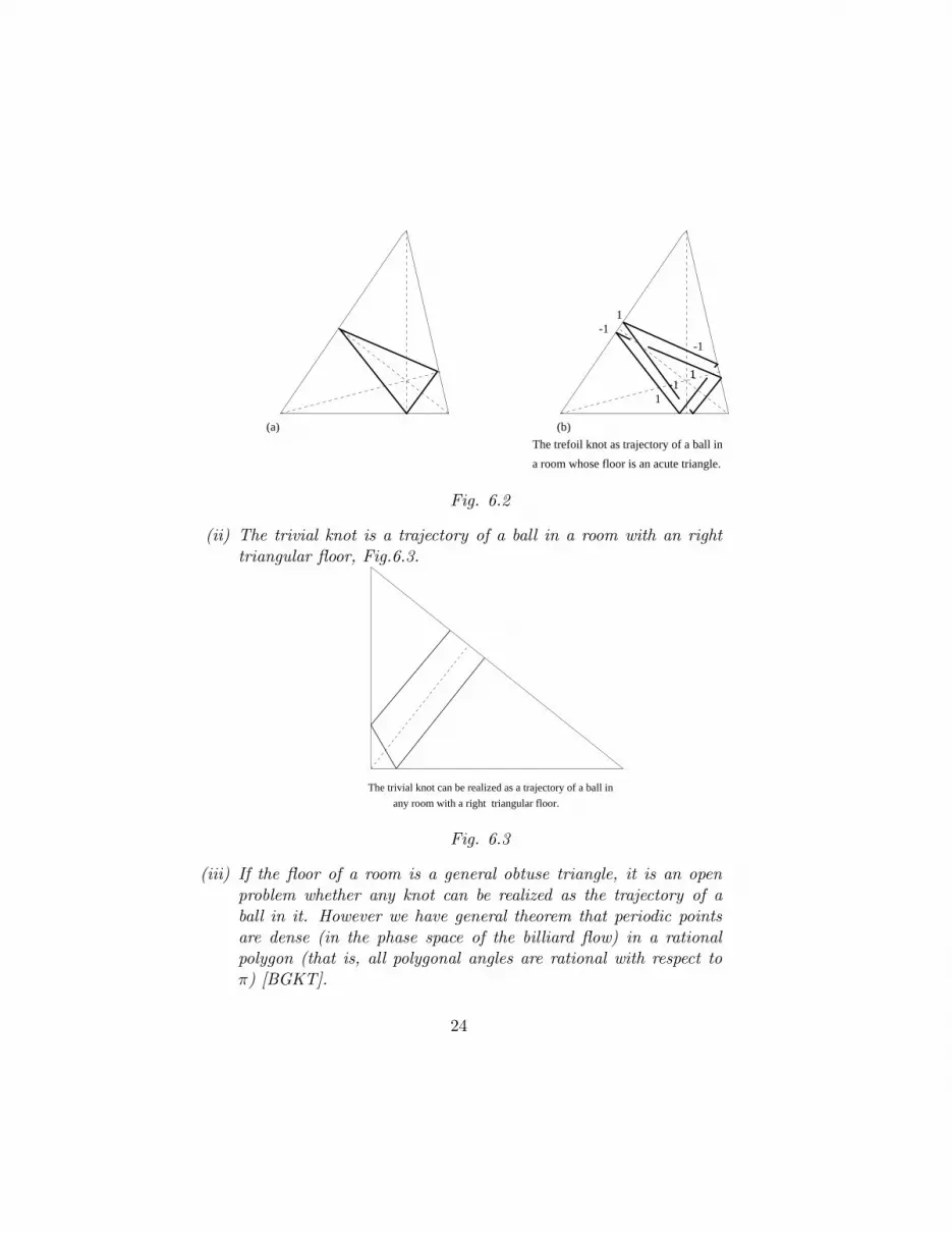
Example 6.2 (i) The trivial knot and the trefoil knot are the trajec-tories of a ball in a room (prism) with an acute triangular floor.In Fig.6.2(a), the diagram of the trivial knot is an inscribed trian-gle ∆I whose vertices are the feet of the triangle’s altitudes. If wemove the first vertex of ∆I slightly, each of its edges splits into twoand we get the diagram of the trefoil. We should be careful withthe altitude of the trajectory: We start from level 1 at the vertexclose to the vertex of ∆I and opposite to the shortest edge of ∆I .Then we choose the vertical parameter so that the trajectory has3 maxima and three minima (Fig.6.2(b)).

23

1

11

1

-1

-1

-1

(b)(a)

The trefoil knot as trajectory of a ball in

a room whose floor is an acute triangle.

Fig. 6.2

(ii) The trivial knot is a trajectory of a ball in a room with an righttriangular floor, Fig.6.3.

The trivial knot can be realized as a trajectory of a ball in

any room with a right triangular floor.

Fig. 6.3

(iii) If the floor of a room is a general obtuse triangle, it is an openproblem whether any knot can be realized as the trajectory of aball in it. However we have general theorem that periodic pointsare dense (in the phase space of the billiard flow) in a rationalpolygon (that is, all polygonal angles are rational with respect toπ) [BGKT].

24

Example 6.2(i) is of interest because it was shown in [BHJS] that thetrefoil knot is not a Lissajous knot and thus it is not a trajectory ofa ball in a room with a rectangular floor. More generally we show inSection 3 that no nontrivial torus knot is a Lissajous knot. However, wecan construct infinitely many torus knots in prisms and in the cylinder.

Example 6.3 (i) Any torus knot (or link) of type (n, 2) can be re-alized as a trajectory of a ball in a room whose floor is a regularn-gon (n ≥ 3). Fig.6.1 shows the (3, 2) torus knot (trefoil) in theregular triangular prism; Fig.6.4(a) depicts the (4, 2) torus link inthe cube; and Fig.6.4(b)(c) illustrates the (5, 2) torus knot in aroom with a regular pentagonal floor.

1

-1

1

-1

1-1

1

-1

1

-1

0

0

00

0

1

1

1

1

1

-1

-1

-1

-1-1

(c)(b)

1

1

1

1

-1

-1

The (4,2) torus link in a cube

-1

-1

(a)

The torus knot of type (5,2) as a trajectory of a ball in a room with a regular pentagonal floor.

Fig. 6.4

(ii) The (4, 3) torus knot is a trajectory of a ball in a room with theregular octagonal floor; Fig.6.5(a).

25

1

1

1

1

-1

-1-1

-1

0

0

0

0

0

0

0

0

0

0

0

0

0

0

1

1

1

1

1

1

1

1

-1

-1-1

-1

-1

-1

-1

-1

0

0

(a) (b)

The torus knot of type (8,3) as a trajectory of a ball in The torus knot of type (4,3) as a trajectory of a ball

in a room with a regular octagonal floor. a room with a regular octagonal floor.

Fig. 6.5

(iii) Figures 6.5(b) and 6.6 illustrate how to construct a torus knot (orlink) of type (n, 3) in a room with a regular n-gonal floor for n ≥ 7.

(iv) Any torus knot (or link) of type (n, k), where n ≥ 2k + 1, can berealized as a trajectory of a ball in a room with a regular n-gonalfloor. The pattern generalizes that of Figures 6.4(b), 6.5(b) and6.6. Edges of the diagram go from the center of the ith edge to thecenter of the (i + k)th edge of the n-gon. The ball bounces fromwalls at altitude 0 and its trajectory has n maxima and n minima.The whole knot (or link) is n-periodic.

26

0

0

0

00

0

0

0

0

00 0

0

0

1

1

1

1

1

1

11

-1

-1

-1

-1

-1

-1

-1

The torus knot of the type (7,3) realized as a trajectory of a ball in a room

with a regular heptagonal floor.

Fig. 6.6

Example 6.4 Let D be a closed billiard trajectory on a 2-dimensionalpolygonal table. If D is composed of an odd number of segments, then wecan always find the “double cover” closed trajectory D(2) in the neigh-borhood of D (each segment will be replaced by two parallel segmentson the opposite sides of the initial segment). This idea can be used toconstruct, for a given billiard knot K in a polygonal prism (the projec-tion D of K having an odd number of segments), a 2-cable K(2) of Kas a billiard trajectory (with projection D(2)). This idea is illustrated inFig.6.1 and 6.4(c) (the (5,2) torus knot as a 2-cable of a trivial one).Starting from Example 2.3(iv) we can construct a 2-cable of a torus knotof the type (n, k) in a regular n-gonal prism, for n odd and n ≥ 2k + 1.

It follows from [BHJS] that 3-braid alternating knots of the form(σ1σ

−12 )2k are not Lissajous knots as they have a non-zero Arf invariant

27

(Corollary 6.12). For k = 1 we have the figure eight knot and for k = 2the 818 knot [Ro].

Example 6.5 (i) The Listing knot (figure eight knot) can be realizedas a trajectory of a ball in a room with a regular octagonal floor,Fig. 6.7.

(ii) Fig.6.8 describes the knot 818 as a trajectory of a ball in a roomwith a regular octagonal floor. This pattern can be extended toobtain the knot (or link) which is the closure of the three braid(σ1σ

−12 )2k in a regular 4k-gonal prism (k > 1).

1

-s

-1

s

-s

-s

s-s

s

(b)

-1

s

(a)

1

1

-1

1

-1

The Listing (figure eight) knot as a trajectory of a ball in a room with a regular octagonal floor.

Fig. 6.73

3Added for e-print: the journal version of the paper illustrates Fig.6.7 by computergraphics generated by Mike Veve.

28

18

-1

1

1

-1

1

-1

1

-1

a room with a regular octagonal floor.

The knot 8 [Ro], realized as a trajectory of a ball in

Fig. 6.8

In the example below we show that the cylinder D2× [−1, 1] supportan infinite number of different knot types (in the case of a cube it wasshown in [La]).

Example 6.6 (i) Any torus knot (or link) of type (n, k), where n ≥2k + 1, can be realized as a trajectory of a ball in the cylinder;compare Fig.6.4(b), Fig.6.5(b) and Fig.6.6.

(ii) Every knot (or link) which is the closure of the three braid (σ1σ−12 )2k

can be realized as the trajectory of a ball in the cylinder. See Fig.6.7(b) for the case of k = 1 (Listing knot) and Fig. 6.8 for thecase of k = 2 and the general pattern.

Any type of knot can be obtained as a trajectory of a ball in somepolyhedral billiard (possibly very complicated). To see this, consider apolygonal knot in R3 and place “mirrors” (walls) at any vertex, in sucha way that the polygon is a “light ray” (ball) trajectory.

Conjecture 6.7Any knot type can be realized as the trajectory of a ball in a polytope.

29

Conjecture 6.8Any polytope supports an infinite number of different knot types.

Problem 6.9

1. Is there a convex polyhedral billiard in which any knot type can berealized as the trajectory of a ball?

2. Can any knot type be realized as the trajectory of a ball in a roomwith a regular polygonal floor?

3. Which knot types can be realized as trajectories of a ball in a cylin-der (D2 × [−1, 1])?

The partial answer to 6.9(3.) was given in [J-P] and [L-O]. In particularLamm and Obermeyer have shown that not all knots are knots in acylinder (e.g. 52 and 810 are not cylinder knots). The new interestingfeature of [L-O] is the use of ribbon condition.

Below we list some information on Lissajous knots (or equivalentlybilliard knots in a cube).

Theorem 6.10 ([BHJS]) An even Lissajous knot is 2-periodic and anodd Lissajous knot is strongly + amphicheiral. A Lissajous knot is calledodd if all, ηx, ηy and ηz are odd. Otherwise it is called an even Lissajousknot.

Theorem 6.11 ([J-P]) In the even case the linking number of the axisof the Z2-action with the knot is equal to ±1.

Corollary 6.12 (i) ([BHJS].) The Arf invariant of the Lissajousknot is 0.

(ii) ([J-P]) A nontrivial torus knot is not a Lissajous knot.

(iii) ([J-P]) For ηz = 2 a Lissajous knot is a two bridge knot and itsAlexander polynomial is congruent to 1 modulo 2.

30

Theorem 6.13 ([La]) Let ηx, ηy > 1 be relatively prime integers andK the Lissajous knot with ηz = 2ηxηy − ηx − ηy and φx = 2ηx−1

2ηzπ,

φy = π2ηz

, φz = 0.Then the Lissajous diagram of the projection on the x − y plane isalternating. Above knots form an infinite family of different Lissajousknots.

Motivated by the case of 2-periodic knots we propose

Conjecture 6.14Turks head knots, (e.g. the closure of the 3-string braids (σ1σ

−12 )2k+1),

are not Lissajous. Observe that they are strongly + amphicheiral.

We do not think, as the above conjecture shows, that the converseto Theorem 6.11 holds. However for 2-periodic knots it may hold (themethod sketched in Section 0.4 of [BHJS] may work).

Problem 6.15Let K be a Z2-periodic knot, such that the linking number of the axis ofthe Z2-action with K is equal to ±1. Is K an even Lissajous knot?

The first prime knots (in the knot tables [Ro]) which may or may notbe Lissajous are 83, 86 (75 is constructed in [La]).

7 Applications and Speculations

A lot can be said about the structure of a manifold by studying its sym-metries. The existence of Zr action on a homology sphere is reflected inthe Reshetikhin-Turaev-Witten invariants. In our description we follow[K-P]. Let M be a closed connected oriented 3-manifold represented asa surgery on a framed link L ⊂ S3. Let r ≥ 3, and set the variable Aused in the Kauffman skein relation to be a primitive root of unity oforder 2r. In particular, A2r = 1. Recall that the invariant Ir(M) isgiven by:

Ir(M) = κ−3σLηcom(L)[L(Ωr)] (2)

31

In L(Ω) each component of L is decorated by an element Ω from theKauffman bracket skein module of a solid torus (see Proposition 7.3):

Ωr =

[(r−3)/2]∑

i=0

[ei]ei

Elements ei satisfy the recursive relation:

ei+1 = zei − ei−1

where z can be represented by a longitude of the torus, and e0 = 1, e1 =z. The value of the Kauffman bracket skein module of the skein elementei, when the solid torus is embedded in S3 in a standard way, is givenby [ei] = (−1)i A2i+2−A−2i−2

A2−A−2 . [ei] is the version of the Kauffman bracket,

normalized in such a way that [∅] = 1 and [L] = (−A2 − A−2)〈L〉. Inthe equation (2), η is a number which satisfies η2[Ωr] = 1, and κ3 is aroot of unity such that

κ6 = A−6−r(r+1)/2.

Finally, σL denotes the signature of the linking matrix of L.

Theorem 7.1 (K-P)Suppose that M is a homology sphere and r is an odd prime. If M isr-periodic then

Ir(M)(A) = κ6j · Ir(M)(A−1) mod (r)

for some integer j.

Theorem 7.1 holds also for Zr-homology spheres.Skein modules can be thought as generalizations to 3-manifolds of

polynomial invariants of links in S3. Our periodicity criteria (especiallywhen link and its quotient under a group action are compared), can bethought as the first step toward understanding relations between skeinmodules of the base and covering space in a covering. We will considerhere the Kauffman bracket skein module and the relation between abase and covering space in the case of the solid torus.

32

Definition 7.2 ([P-2, H-P-2])Let M be an oriented 3-manifold, Lfr the set of unoriented framed linksin M (∅ allowed), R = Z[A±1, and RLfr the free R module with basisLfr. Let S2,∞ be the submodule of RLfr generated by skein expressionsL+−AL0−A−1L∞, where the triple L+, L0, L∞ is presented in Fig.7.1,and L ⊔ T1 + (A2 + A−2)L, where T1 denotes the trivial framed knot.We define the Kauffman bracket skein module (KBSM), S2,∞(M), asthe quotient S2,∞(M) = RLfr/S2,∞.

LLL 80+

Fig. 7.1.

Notice that L(1) = −A3L in S2,∞(M); we call this the framing relation.In fact this relation can be used instead of L⊔T1+(A2+A−2)L relation.

Proposition 7.3 ([H-P-1, P-2])The KBSM of a solid torus (presented as an annulus times an interval),is an algebra generated by a longitude of the solid torus; it is Z[A±1]algebra isomorphic to Z[A±1][z] where z corresponds to the longitude.

Let the group Zr acts on the solid torus (S1 × [1/2, 1])× [0, 1]) withthe generator ϕ(z, t) = (e2πi/rz, t). where z represents an annulus pointand t an interval point. Let p be the r-covering map determined by theaction (see Fig. 7.2). We have the “transfer” map p−1

∗ from the KBSMof the base to the KBSM of the covering space (modulo r) due to thegeneralization of Lemma 3.2. where z represent an annulus point andt an interval point. To present the generalization in the most naturalsetting we introduce the notion of the “moduli” equivalence of links andassociated moduli skein modules.

33

... ...

...

...

...

...

..

.

... ...

p

ϕ

L

L*

Fig. 7.2

Definition 7.4 (i) We say that two links in a manifold M are moduliequivalent if there is a preserving orientation homeomorphism ofM sending one link to another.

(ii) Let G be a finite group action on M . We say that two links L andL′ in M are G moduli equivalent if L′ is ambient isotopic to g(L)for some g ∈ G.

(ii) We define moduli KBSM (resp. G moduli KBSM) as KBSM di-vided by moduli (resp. G moduli) relation. We would use thenotation Sm

2,∞(M) (resp. SG2,∞(M)).

Lemma 7.5 Let the group Zr, r prime, act on the oriented 3-manifoldM and let L = Lsym(cr) be a framed singular link in M which satisfies

34

ϕ(L) = L where ϕ : M → M is the generator of the Zr-action, and Zr

has no fixed points on L. Then in the skein module SZr2,∞(M) one has

the formula

Lsym( )

≡ ArLsym( )

+ A−rLsym( )

mod r

where Lsym( )

, Lsym( )

and Lsym( )

denote three ϕ-invariant dia-

grams of links which are the same outside of the Zr-orbit of a neigh-borhood of a fixed singular crossing at which they differ by replacing

Lsym(cr) by or , or , respectively.Notice that in the case of an action on the solid torus, ϕ is isotopic toidentity, thus Zr moduli KBSM is the same as KBSM.

We can use Lemma 7.5 to find the formula for a torus knot in a solidtorus modulo r, for a prime r.

Theorem 7.6 The torus knot Tr,k satisfies:

T (r, k) = Ar(k−1)(xk+1 − x−k−1 − A−4r(xk−1 − x1−k)

x − x−1)

where z = x + x−1 is a longitude of the solid torus (an annulus timesan interval).

One can prove Theorem 7.6 by rather involved induction4 (compareexample 7.7), however modulo r Theorem 7.6 has very easy proof us-ing Lemma 7.5. Namely Tr,k is an r cover of a knot T1,k and for T1,k

one has T1,k+2 = A(x + x−1)T1,k+1 − A2T1,k in KBSM, thus T1,k =

A(k−1)(xk+1−x−k−1−A−4(xk−1−x1−k)x−x−1 ) Now one compares binary computa-

tional trees of T1,k and Tr,k (modulo r) using lemma 7.5, to get mod rversion of Theorem 7.6.In fact for any regular r covering p : M → M∗ we have the transfer map( mod r):

p−1∗ : S2,∞(M∗) → SZr

2,∞(M) mod r

which is a Z homomorphism and p−1∗ (w(A)L) ≡ w(Ar)p−1(L) mod r.

4Added for e-print: The formula has been generalized and given a simple ideolog-ical proof in R.Gelca, C.Frohman, Skein Modules and the Noncommutative Torus,Transactions of the AMS, 352, 2000, 4877-4888.

35

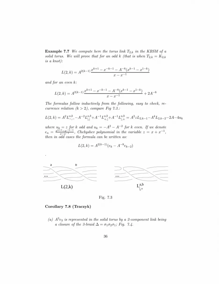
Example 7.7 We compute here the torus link T2,k in the KBSM of asolid torus. We will prove that for an odd k (that is when T2,k = K2,k

is a knot):

L(2, k) = A2(k−1) xk+1 − x−k−1 − A−8(xk−1 − x1−k)

x − x−1

and for an even k:

L(2, k) = A2(k−1) xk+1 − x−k−1 − A−8(xk−1 − x1−k)

x − x−1+ 2A−6

The formulas follow inductively from the following, easy to check, re-currence relation (k > 2), compare Fig 7.3.:

L(2, k) = A2La,b−,−−A−2La,b

|,| +A−1La,b+,|+A−1La,b

|,+ = A2zL2,k−1−A4L2,k−2−2A−4uk

where uk = z for k odd and uk = −A2 − A−2 for k even. If we denoteen = xn+1−x−n−1

x−x−1 , Chebyshev polynomial in the variable z = x + x−1,then in odd cases the formula can be written as:

L(2, k) = A2(k−1)(ek − A−8ek−2)

.

... ...

La,b|,+

a b

L(2,k)

Fig. 7.3

Corollary 7.8 (Traczyk)

(a) A3e3 is represented in the solid torus by a 2-component link beinga closure of the 3-braid ∆ = σ1σ2σ1; Fig. 7.4.

36

(b) In S3, the closed braid links ∆2n+1 form an infinite family of(simple) links whose Jones polynomial differ only by an invert-

ible element5 in Z[t±12 ].

(c) There are infinite families of links sharing the same Jones poly-nomial (e.g. t2 + 2 + t−2)).

L(2,3) = A (e - A e ) = 4 -8

3= A

-A -1 ∆ -4

1

1 ∆

= A - A e

Fig. 7.4

Proof:

(a) Using the formula of Example we have L2,3 = A4(e3 − A−8e1).The necessary calculation is shown in Fig. 7.4.

(b) e3 is an eigenvector of the Dehn twist on the solid torus and anybraid, γ, is changed by a Dehn twist to ∆2γ. Thus ∆2n+1 = A6n∆in the KBSM of the solid torus.Closed braids ∆2n+1 form an infinite family of different 2-componentlinks in S3 (linking number equal to k).

(c) Consider a connected sum of ∆2n+1 and ∆2m+1. For fixed n + mone has an infinite family of different 3-component links with thesame Jones polynomial. For m = −n−1 one get the family of linkswith the Jones polynomial of the connected sum of right handedand left handed Hopf links (thus (t + t−1)2).

2

We do not know which en can be realized by framed links in a solidtorus, however we have:

5Added for e-print: P.Traczyk, 3-braids with proportional Jones polynomials,Kobe J. Math., 15(2), 1998, 187-190.

37

Lemma 7.9 If en is realized by a framed link then n = 2k − 1 for somek.

Proof: Consider the standard embedding of a solid torus in S3. Then< en >A=−1= (−1)n−1 n+1

2 on the other hand for a link L one has

< L >−1= (−2)com(L)−1. Thus n = 2k − 1 2

References

[Bi] J.S.Birman, Braids,Links and mapping class groups, Ann.Math.Studies 82, Princeton N.J.: Princeton Univ. Press, 1974.

[BGKT] M.Boshernitzan, G.Galperin, T.Kroger, S.Troubetzkoy, Someremarks on periodic billiard orbits in rational polygons, preprint,SUNY Stony Brook, 1994.

[BHJS] M.G.V. Bogle, J.E. Hearst, V.F.R. Jones, L. Stoilov, Lissajousknots, Journal of Knot Theory and Its Ramifications, 3(2), 1994,121-140.

[B-L-M] R. D. Brandt, W. B. R.Lickorish, K. C. Millett, A polynomialinvariant for unoriented knots and links, Invent. Math., 84 (1986),563-573.

[Bu] W.Burau, Uber Zopfgruppen und gleichsinnig verdrillte Verket-tungen, Abh. Math. Sem. Hansischen Univ., 11, 171-178, 1936.

[D-T] C. H. Dowker, M. B. Thistlethwaite, Classification of knot projec-tions, Topology and its applications 16 (1983), 19-31, and Tablesof knots up to 13 crossings (computer printout).

[Ho] C. F. Ho, A new polynomial for knots and links; preliminary re-port. Abstracts AMS 6(4) (1985), p 300.

[H-K] R.Hartley, A.Kawauchi, Polynomials of amphicheiral knots,Math. Ann., 243, 1979, 63-70.

[H-P-1] J. Hoste, J.H. Przytycki, An invariant of dichromatic links,Proc. Amer. Math.Soc., 105(4) 1989, 1003-1007.

38

[H-P-2] J. Hoste, J.H. Przytycki, A survey of skein modules of 3-manifolds, in Knots 90, Proceedings of the International Confer-ence on Knot Theory and Related Topics, Osaka (Japan), August15-19, 1990, Editor A. Kawauchi, Walter de Gruyter 1992, 363-379.

[Jo] V. Jones, Hecke algebra representations of braid groups and linkpolynomials, Ann. of Math. (1987) 335-388.

[Ka] L.H. Kauffman, An invariant of regular isotopy, Trans. Amer.Math. Soc., 318(2), 1990, 417–471.

[J-P] V.F.R.Jones, J.H.Przytycki, Lissajous knots and billiard knots,Banach Center Publications, Vol. 42, Knot Theory, 1998, to ap-pear.

[K-P] J.Kania-Bartoszynska, J.H.Przytycki, 3-manifold invariants andperiodicity of homology spheres, preprint 1997.(Added for e-print: The final version of the paper is:P.Gilmer, J.Kania-Bartoszynska, J.H.Przytycki, 3-manifold in-variants and periodicity of homology spheres, Algebraic and Geo-metric Topology 2, 2002, 825-842.http://xxx.lanl.gov/abs/math.GT/9807011).

[La] C.Lamm, There are infinitely many Lissajous knots, ManuscriptaMathematica, 93, 1997, 29-37.

[L-O] C.Lamm, D.Obermeyer, A note on billiard knots in a cylinder,preprint, October 1997.

[Li] W.B.R.Lickorish. Polynomials for links.Bull. London Math. Soc.20 (1998) 558-588.

[L-M] W.B.R. Lickorish, K. Millett, A polynomial invariant of orientedlinks, Topology 26(1987), 107-141.

[Mu-1] K. Murasugi, On periodic knots, Comment Math. Helv.,46(1971), 162-174.

[Mu-2] K. Murasugi, Jones polynomials of periodic links, Pac. J. Math.,131 (1988), 319-329.

39

[Na] S.Naik, New invariants of periodic knots, Math. Proc. CambridgePhilos. Soc. 122 (1997), no. 2, 281–290.

[Per] K.A.Perko, Invariants of 11-crossing knots, Publications Math.d’Orsay, 1980.

[P-1] J.H.Przytycki, Survey on recent invariants in classical knot theory,Warsaw University Preprints 6,8,9; 1986.

[P-2] J.H.Przytycki, Skein modules of 3-manifolds, Bull. Ac. Pol.:Math.; 39(1-2), 1991, 91-100.

[P-3] J.H.Przytycki, On Murasugi’s and Traczyk’s criteria for periodiclinks. Math Ann., 283 (1989) 465-478.

[P-4] J.H.Przytycki, Vassiliev-Gusarov skein modules of 3-manifoldsand criteria for periodicity of knots, Low-dimensional topology(Knoxville, TN, 1992), 143–162, Conf. Proc. Lecture Notes Geom.Topology, III, Internat. Press, Cambridge, MA, 1994.

[P-5] J.H.Przytycki, An elementary proof of the Traczyk-Yokota criteriafor periodic knots, Proc. Amer. Math. Soc. 123 (1995), no. 5,1607–1611.

[Ro] D. Rolfsen, Knots and links. Publish or Perish, 1976.

[Sm] The Smith Conjecture (J.W.Morgan, H.Bass). New York Aca-demic Press 1984.

[Ta] S.Tabachnikov, Billiards Panor. Synth. No. 1, 1995, vi+142 pp.

[Thur] W.Thurston, The Geometry and Topology of 3-manifolds,Mimeographed notes, 1977-1979.

[T-1] P.Traczyk, 10101 has no period 7: a criterion for periodic links,Proc. Amer. Math. Soc. 180 (1990) 845-846.

[T-2] P.Traczyk, A criterion for knots of period 3, Topology Appl. 36(1990), no. 3, 275–281.

[T-3] P.Traczyk, Periodic knots and the skein polynomial, Invent.Math., 106(1), (1991), 73-84.

40

[Ve] D.L.Vertigan. On the computational complexity of Tutte, Jones,Homfly and Kauffman invariants. PhD. thesis, 1991.

[We] Hermann Weyl, Symmetry, Princeton University Press, 1952.

[Yo-1] Y.Yokota, The Jones polynomial of periodic knots, Proc. Amer.Math. Soc. 113 (1991), no. 3, 889–894.

[Yo-2] Y.Yokota, The skein polynomial of periodic knots, Math. Ann.,291 (1991), 281-291.

[Yo-3] Y.Yokota, The Kauffman polynomial of periodic knots, Topology32 (1993), no. 2, 309–324.

[Yo-4] Y.Yokota, Polynomial invariants of periodic knots, J. Knot The-ory Ramifications 5 (1996), no. 4, 553–567.

Address:Department of MathematicsGeorge Washington UniversityWashington, DC 20052e-mail: przytyck@math.gwu.eduprzytyck@gwu.edu

41