Seediscussions,stats,andauthorprofilesforthispublicationat:https://www.researchgate.net/publication/265511966

SynergycyclesintheNorwegianinnovationsystem:Therelationbetweensynergyandcyclevalues

ARTICLEinSSRNELECTRONICJOURNAL·SEPTEMBER2014

DOI:10.2139/ssrn.2492456·Source:arXiv

CITATION

1

READS

32

3AUTHORS:

IngaA.Ivanova

FarEasternFederalUniversity

14PUBLICATIONS62CITATIONS

SEEPROFILE

ØivindStrand

AalesundUniversityCollege

19PUBLICATIONS70CITATIONS

SEEPROFILE

LoetLeydesdorff

UniversityofAmsterdam

570PUBLICATIONS14,758CITATIONS

SEEPROFILE

Allin-textreferencesunderlinedinbluearelinkedtopublicationsonResearchGate,

lettingyouaccessandreadthemimmediately.

Availablefrom:LoetLeydesdorff

Retrievedon:04February2016

1

Synergy cycles in the Norwegian innovation system:

The relation between synergy and cycle values

Inga Ivanova1, Øivind Strand

2, & Loet Leydesdorff

3

Abstract

The knowledge base of an economy measured in terms of Triple-Helix relations can be analyzed

in terms of mutual information among geographical, sectorial, and size distributions of firms as

dimensions of the probabilistic entropy. The resulting synergy values of a TH system provide

static snapshots. In this study, we add the time dimension and analyze the synergy dynamics

using the Norwegian innovation system as an example. The synergy among the three dimensions

can be mapped as a set of partial time series and spectrally analyzed. The results suggest that the

synergy at the level of both the country and its 19 counties shows non-chaotic oscillatory

behavior and resonates in a set of natural frequencies. That is, synergy surges and drops are non-

random and can be analyzed and predicted. There is a proportional dependence between the

amplitudes of oscillations and synergy values and an inverse proportional dependency between

the oscillation frequencies‟ relative inputs and synergy values. This analysis of the data informs

us that one can expect frequency-related synergy-volatility growth in relation to the synergy

value and a shift in the synergy volatility towards the long-term fluctuations with the synergy

growth.

Keywords: knowledge base, probabilistic entropy, triple helix, spectral analysis

1. Introduction

Multi-dimensional systems of various types, such as social or biological, can be

considered eco-systems, that can flourish if uncertainty in the relations among constituent parts is

reduced (Ulanowicz, 1986). The Triple Helix (TH) model of university-industry-government

1 School of Business and Public Administration, Far Eastern Federal University, 8, Sukhanova St., Vladivostok

690990, Russia; inga.iva@mail.ru 2 Aalesund University College, Department of International Marketing, PO Box 1517, 6025 Aalesund, Norway; +47

70 16 12 00; ost@hials.no 3 University of Amsterdam, Amsterdam School of Communication Research (ASCoR), PO Box 15793, 1001

NG Amsterdam, The Netherlands; loet@leydesdorff.net

2

relations can serve as a specific example of such systems. Mutual information in three or more

dimensions can be considered a reduction of uncertainty at the system level or a measure of

synergy, and can be expressed in terms of bits of information using the Shannon-formulas

(Abramson, 1963; Theil, 1972; Leydesdorff, 1995).

The synergy of a TH system can be measured as reduction of uncertainty using mutual

information among the three dimensions of firm sizes, the technological knowledge bases of

firms, and geographical locations. Mutual information can be expressed in bits of information

using the formalisms of Shannon‟s information theory. One should note that the three

dimensions refer to different institutional actors and are functionally differentiated. Because of

the additive character of entropy the system of university-industry-government relations can

graphically be displayed in the form of a Venn diagram with each surface area corresponding to

the expected information content (Fig. 1).

Fig. 1 Venn diagram of university (U) –industry (I) –government (G) relations. The central

overlapping part UIG corresponds to the three-lateral mutual information.

The problem in applying Shannon formalism to three-lateral and higher-order

dimensional interactions is that mutual information is then a signed information measure (Yeung

2008, Leydesdorff 2010). A negative information measure cannot comply with Shannon‟s

G

U I

UG

UI

IG UIG

3

definition of information (Krippendorff 2009a, b). This contradiction can be solved by

considering mutual information as different from mutual redundancy (Leydesdorff & Ivanova,

2014). In the three-dimensional case, however, mutual information is equal to mutual

redundancy and, thus, can be considered a Triple-Helix indicator of synergy in university-

industry-government relations (Leydesdorff et al, 2014).

A number of studies have been devoted to measuring synergy across different countries

and regions, such as the Netherlands (Leydesdorff, Dolfsma, & Van der Panne, 2006), Germany

(Leydesdorff & Fritsch, 2006), Hungary (Lengyel & Leydesdorff, 2011), Norway (Strand &

Leydesdorff, 2013), Sweden (Leydesdorff & Strand, 2012), West Africa (Mêgnigbêto, 2013),

China (Leydesdorff & Zhou, 2014), and Russia (Leydesdorff, Perevodchikov, & Uvarov, in

press). One obtains maps of synergy distribution across the territory. However, having only these

synergy “snapshots”, one is unable to answer a series of questions, such as what is the temporal

character of synergy evolution, and does the synergy value affect its temporal evolution? Note

that a TH cannot be static (Etzkowitz & Leydesdorff, 2000). Rather it is an ever-evolving

system, and therefore one can expect that the synergy in this system also evolves with the

passage of time.

The core research questions of the present paper regarding temporal synergy evolution

are as follows: how does the synergy evolve (e.g., is there a trend-like, chaotic, oscillatory, or

some other functional dependency)? Do synergy values affect the temporal evolution (i.e. is

there a difference in synergy evolution between high and low synergy). And can we provide

numerical indicators of synergy evolution? Answering these questions may shed light on the

control mechanisms of a system and provide tools for exploring multi-dimensional systems of

this type in different areas.

In this study, we analyze the temporal dynamics of mutual information in the Norwegian

innovation system as an example. The choice of the Norwegian innovation system is guided by

the ready availability of data. However, the method is generic and can be applied to any data for

time series that fulfill the criterion of possessing three (or more) different dimensions. The paper

is structured as follows. Section 2 describes the method. The results are presented in Section 3

and discussed in Section 4. Finally some conclusions and policy implications are formulated in

Section 5.

4

2. Methods and data

2.1 Methods

The synergy of interaction between two actors can be numerically evaluated using the

formalisms of Shannon‟s information theory by measuring mutual information as the reduction

of uncertainty. In the case of three interacting dimensions, the mutual (configuration)

information can be defined by analogy with mutual information in two dimensions, as follows

(Abramson, 1963; McGill, 1954):

(1)

Here, , , denote probabilistic entropy measures in one, two, and three dimensions:

∑

∑ (2)

∑

The values of p represent the probabilities, which can be defined as the ratio of the

corresponding frequency distributions:

⁄

⁄

⁄ (3)

5

is the total number of events, and , , denote the numbers of events relevant in

subdivisions. For example, if N is the total number of firms, is the number of firms in the i -

th county, the j-th organizational level (defined by the number of staff employed), and the k-th

technology group. Then and can be calculated as follows:

∑ ; ∑

A set of L mutual information values for a certain time period, considered as a finite time

signal, can be spectrally analyzed with the help of the discrete Fourier transform (Kester, 2000):

∑ (4)

Here:

(5)

The Fourier decomposition by itself cannot provide us with information regarding synergy

evolution except the values of the spectral coefficients , , and . Because the aggregate

(country-related) synergy is determined by additive entropy measures (Eq. (1)), it can also be

decomposed as a sum of partial (county-related) synergies :

(6)

So that each partial synergy can be written in the same form as Eq. (4):

This decomposition is different from that used in our previous studies (e.g., Leydesdorff & Strand, 2013; Strand &

Leydesdorff, 2013).

6

∑

∑

(7)

…

∑

Here:

After substituting Eqs. (4) and (7) into (6) and re-grouping the terms, one obtains:

(8)

Leydesdorff and Ivanova (2014) showed that mutual information in three dimensions is

equal to mutual redundancy ( ). Aggregated redundancy can equally be decomposed

as a sum of partial redundancies, corresponding to the geographical, structural, or technological

dimensions of the innovation system under study. Mutual redundancy changes over time, so that

one can write:

7

(9)

In another context, Ivanova & Leydesdorff (2014 b) expressed the redundancy that can be

obtained as follows (i= 1, 2 … n):

(10)

The oscillating function in Eq. (10) can be considered a natural frequency of the TH

system. This natural frequency is far from fitting observed redundancy values for .

However, real data for the definite time interval can be fit with the help of the discrete Fourier

transform, comprising a finite set of frequencies. Each frequency in the set composing Eq. (9)

can be considered a natural frequency of the TH system:

∑ (11)

Comparing Eq. (11) with Eq. (10) one can approximate the empirical data for three-

dimensional redundancy as a sum of partial redundancies corresponding to frequencies

that are multiples of the basic frequency: w, 2w, 3w … etc.

(12)

In other words, a TH system can be represented as a string resonating in a set of natural

frequencies with different amplitudes. Frequency-related amplitudes, which can be defined as

8

modules of the corresponding Fourier coefficients, can be considered the spectral structure of the

TH system. Absolute values of the Fourier-series coefficients can be defined as follows

√

(13)

These coefficients determine the relative contributions of the harmonic functions with

corresponding frequencies to the aggregate redundancy (R123 in Eq. (11)).

2.2 Data

Norwegian establishment data were retrieved from the database of Statistics Norway at

https://www.ssb.no/statistikkbanken/selecttable/hovedtabellHjem.asp?KortNavnWeb=bedrifter&

CMSSubjectArea=virksomheter-foretak-og-regnskap&PLanguage=1&checked=true. The data

include time series of Norwegian companies for the period 2002-2014, and encompass

approximately 400,000 firms per year. The data include the number of establishments in the

three relevant dimensions: geographical (G), organizational (O), and technological (T).

Nineteen counties are distinguished in the geographical dimension. In the organizational

dimension, establishments are subdivided with reference to different numbers of employees by

eight groups: no-one employed; 1-4 employees; 5-9 employees; 10-19 employees; 20-49

employees; 50-99 employees; 100-249 employees; and 250 or more employees. The number of

employees can be expected to correlate with the establishment‟s organizational structure.

The technological dimension indicates domains of economic activity. The data for the

period 2002-2008 were organized according to the NACE Rev. 1.1 classification, and the data

for the period 2009-2014 were organized according to the NACE Rev. 2 classification. Some of

the criteria for construction of the new classification, were reviewed: but there is no one-to-one

correspondence between NACE Rev. 1.1 (with 17 sections and 62 divisions) and NACE Rev. 2

(with 21 sections and 88 divisions) (EUROSTAT a). To correctly merge the NACE Rev. 1.1 and

9

NACE Rev. 2 data one has to turn to a higher level of aggregation (Appendix B) containing 10

classes (EUROSTAT b).

3. Data analysis

3.1 Descriptive statistics

Country synergy is decomposed as a sum of the synergies at the county level in

accordance with Eq. (6). The results of the calculations for the period 2002-2014 years (in mbits

of information) are shown in Figs 2-6.

Fig. 2 Summary of the development of Norwegian synergy for the period 2002-

2014 (in mbits of information)

-10

-9

-8

-7

-6

-5

-4

-3

-2

-1

0

T(U

IG)

in m

bit

s o

f in

form

atio

n

years

T(UIG)forNorway

10

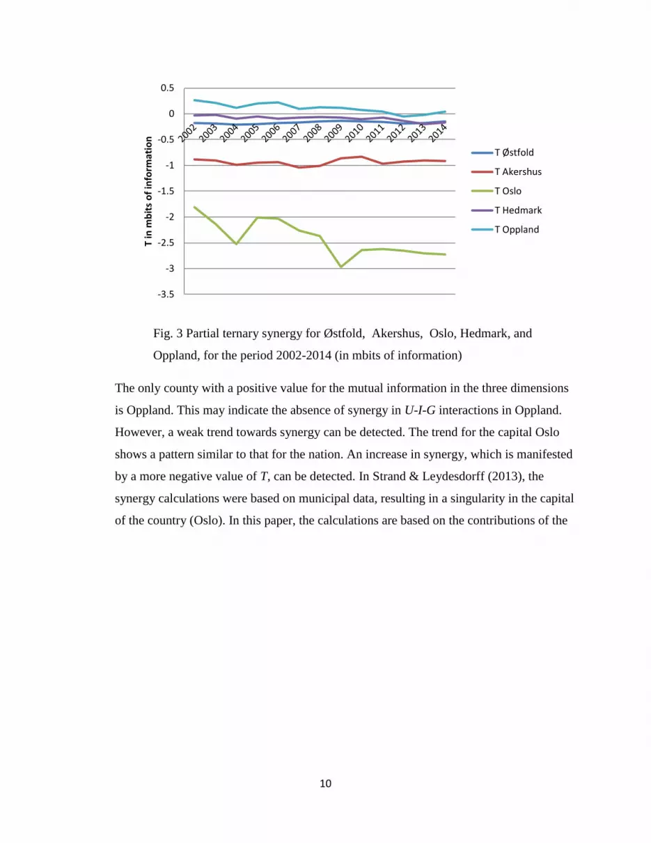
Fig. 3 Partial ternary synergy for Østfold, Akershus, Oslo, Hedmark, and

Oppland, for the period 2002-2014 (in mbits of information)

The only county with a positive value for the mutual information in the three dimensions

is Oppland. This may indicate the absence of synergy in U-I-G interactions in Oppland.

However, a weak trend towards synergy can be detected. The trend for the capital Oslo

shows a pattern similar to that for the nation. An increase in synergy, which is manifested

by a more negative value of T, can be detected. In Strand & Leydesdorff (2013), the

synergy calculations were based on municipal data, resulting in a singularity in the capital

of the country (Oslo). In this paper, the calculations are based on the contributions of the

-3.5

-3

-2.5

-2

-1.5

-1

-0.5

0

0.5

T in

mb

its

of

info

rmat

ion

T Østfold

T Akershus

T Oslo

T Hedmark

T Oppland

11

counties to the national level, allowing the contribution of the capital to be specified.

Fig. 4 Partial ternary synergy for Buskerud, Vestfold, Telemark, Aust-Agder, and

Vest-Agder, for the period 2002-2014 (in mbits of information)

The industrialized counties of Telemark, Buskerud, and Vestfold show a pattern with

decreasing synergy over time. The two Agder counties show an opposite development to the

others with an increase in synergy.

-0.4

-0.35

-0.3

-0.25

-0.2

-0.15

-0.1

-0.05

0T

in m

bit

s o

f in

form

atio

n T Buskerud

T Vestfold

T Telemark

T Aust-Agder

T Vest-Agder

12

Fig. 5 Partial ternary synergy for Rogaland, Hordaland, Sogn og Fjordane, Møre

og Romsdal, and Sør-Trøndelag, for the period 2002-2014 (in mbits of

information)

Rogaland which is dominated by the oil industry, shows a decreasing trend, but the

magnitude of the synergy still exceeds its neighbor Hordaland. The small counties of Sogn and

Fjordane show a trend with increased synergy over time.

-0.8

-0.7

-0.6

-0.5

-0.4

-0.3

-0.2

-0.1

0

T in

mb

its

of

info

rmat

ion

T Rogaland

T Hordaland

T Sogn og Fjordane

T Møre og Romsdal

T Sør-Trøndelag

-0.9

-0.8

-0.7

-0.6

-0.5

-0.4

-0.3

-0.2

-0.1

0

T in

mb

its

of

info

rmat

ion

T Nord-Trøndelag

T Nordland

T Troms Romsa

T Finnmark

13

Fig. 6 Partial ternary synergy for Nord-Trøndelag, Nordland, Troms Romsa, and

Finnmark, for the period 2002-2014 (in mbits of information)

Among the northern counties, Nordland and Finnmark show a development with an increase in

synergy. Fluctuations in synergy data can be interpreted as synergy cycles. Like economic cycles

they may indicate some endogenous characteristics of an innovation system such as cyclic

oscillations of the market system (Morgan, 1991). An alternative to considering the fluctuations

as cycles would be to consider them a result of noise in the data; we clarify this point in the next

section.

3,2 Transmission power and efficiency

Having the transmission time series we calculated the transmission power time series for

Norway as a whole and separately for constituent counties according the following formula

(Mêgnigbêto, 2014, p. 287):

{

(14)

The transmission power was designed to measure the efficiency of the mutual information.

While the transmission defines the total amount of configurational information, the transmission

power represents the share of the synergy actually produced in the system relative to its size. For

positive transmission values, it is simply the ratio of overlapping surface area in the Venn

diagram to the whole surface area of the figure (Fig. 1). Mêgnigbêto (2014, p.290) argued that

“… with such indicators, a same system may be compared over time; different systems may also

be compared”. Figs. 7-11 present the graphs of the transmission power.

14

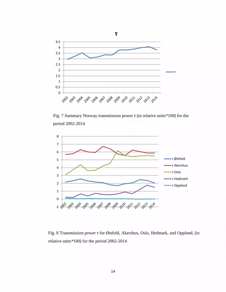
Fig. 7 Summary Norway transmission power τ (in relative units*100) for the

period 2002-2014

Fig. 8 Transmission power τ for Østfold, Akershus, Oslo, Hedmark, and Oppland, (in

relative units*100) for the period 2002-2014

0

0.5

1

1.5

2

2.5

3

3.5

4

4.5

τ

τ

-1

0

1

2

3

4

5

6

7

8

τ Østfold

τ Akershus

τ Oslo

τ Hedmark

τ Oppland

15

Fig. 9 Transmission power τ for Buskerud, Vestfold, Telemark, Aust-Agder, and

Vest-Agder, (in relative units*100) for the period 2002-2014

Fig. 10 Transmission power τ for Rogaland, Hordaland, Sogn og Fjordane, Møre og

Romsdal, and Sør-Trøndelag, (in relative units*100) for the period 2002-2014

0

1

2

3

4

5

6

7

2002200320042005200620072008200920102011201220132014

τ Buskerud

τ Vestfold

τ Telemark

τ Aust-Agder

τ Vest-Agder

0

1

2

3

4

5

6

7

τ Rogaland

τ Hordaland

τ Sogn og Fjordane

τ Møre og Romsdal

τ Sør-Trøndelag

16

Fig.11 Transmission power τ for Nord-Trøndelag, Nordland, Troms Romsa, and

Finnmark, (in relative units*100) for the period 2002-2014

Comparing the national level transmission power in Fig. 7 with the synergy in Fig. 2

shows increased transmission power and increased synergy over time. At the county level, the

same patterns are most pronounced in Oslo, the Agder counties, Sogn og Fjordane, and Nordland

og Finmark.

We compared the percentage of the average efficiency deviation

,

where is the efficiency for the i-th county averaged over the period 2002-2014; is the

summary average efficiency averaged over all of the counties (Fig. 11), and the percentage of

average synergy deviation

, where is the synergy for i-th county

averaged over the period 2002-2014; and is the summary average synergy averaged over all

of the counties (Fig.12). Efficiency is above the country average in Akershus (τ 02), Oslo (τ 03),

Aust-Agder (τ 09), Rogaland (τ 11), Sogn og Fjordane (τ 14), Møre og Romsdal (τ 15), and

Nordland (τ 18), and is extremely high in Finnmark (τ 20). One can observe that the efficiency

and synergy peaks do not coincide. That is counties with the highest synergy values cannot

0

2

4

6

8

10

12

τ Nord-Trøndelag

τ Nordland

τ Troms Romsa

τ Finnmark

17

always be considered the most efficient. This may indicate that the increase in synergy is caused

by increased transmission power.

Fig. 12 Percentage of average efficiency deviation for 19 Norwegian counties for

the period 2002-2014 (in percent)

-150

-100

-50

0

50

100

150

200

1 2 3 4 5 6 7 8 9 10 11 12 13 14 15 16 17 18 19

K

counties

% average efficiency deviation

-200

-100

0

100

200

300

400

500

1 2 3 4 5 6 7 8 9 10 11 12 13 14 15 16 17 18 19

P

counties

% of average synergy deviation

18

Fig. 13 Percentage of average synergy deviation for 19 Norwegian counties for

the period 2002-2014 (in percent)

As a next step, we analyzed aggregate redundancy time series with the help of the

discrete Fourier transform in accordance with Eq. (4). The inputs of different frequency modes to

Norway‟s synergy (w, 2w, 3w, 4w, 5w, 6w), calculated according to Eq. (14), are shown in Fig.

14.

Fig. 14 Modules of Fourier series coefficients C versus frequency for summary

ternary synergy (in mbits of information)

Each of the county-related synergies can be mapped as fluctuations around an average

value. Thus, the average values can be taken as the first terms in the corresponding Fourier

decomposition describing non-fluctuating terms ( in Eq. (7)). These average values form the

synergy line specter.

Having calculated the modules of the Fourier series coefficients, which are the measures

of different frequency modes, as well as the line specter synergy values we can map these

modules versus synergy values to obtain corresponding functional dependencies. Because we

address the real-number data (for the period 2002-2014), then, due to the symmetry of DFT

0

0.05

0.1

0.15

0.2

0.25

1 2 3 4 5 6

mb

its

0f

info

rmat

ion

n

C

19

coefficients, only half the number of input data with different frequency components (the first

six) can be discerned.

In Fig. 15 synergies (in mbits of information) are plotted versus frequency amplitudes (in

mbits of information). It can be seen from the figure that observed synergies can be fitted by

polynomial approximation. The coefficients of determination R2 of the approximation curve for

all of the graphs, except for 2w, are relatively high. The coefficients at the first term, defining

the long-run speed of the corresponding frequency relative to the contribution increase, decreases

from the low-frequency end to the high-frequency end of the specter. Extreme synergy and

Fourier coefficient values are also found for Oslo. The equations in the upper parts of graphs

denote the explicit form of the polynomial approximation

y = 0.2594x2 - 0.0236x + 0.1976

R² = 0.8533

0.00

0.20

0.40

0.60

0.80

1.00

1.20

1.40

1.60

1.80

0.00 1.00 2.00 3.00

C1

mb

its

of

info

rmat

ion

T mbits of information

w

w

polinomialapproximation

y = -0.0304x2 + 0.1144x + 0.0963

R² = 0.1621

0.00

0.05

0.10

0.15

0.20

0.25

0.30

0.00 1.00 2.00 3.00

C2

mb

its

of

info

rmat

ion

T mbits of information

2w

2w

polinomialapproximation

20

Fig. 15 Observed average synergy absolute values (in mbits of

information) versus Fourier coefficients absolute values (in mbits of information)

for the first six frequencies.

The degree of synergy fluctuation randomness can be evaluated using R/S analysis

(Hurst, 1951). The standard algorithm and the calculation results are presented in the Appendix

A. The Hurst rescaled range statistical measure H values in the range 0.5 < H < 1 indicate a

persistent or trend-like behavior described by monotone function. H = 0.5 corresponds to a

y = 0.1902x2 - 0.0137x + 0.075

R² = 0.9266

0.00

0.20

0.40

0.60

0.80

1.00

1.20

1.40

0.00 1.00 2.00 3.00

C3

mb

its

of

info

rmat

ion

T mbits of information

3w 3w

polinomialapproximation

y = 0.0585x2 + 0.1133x + 0.0634

R² = 0.8191

0.00

0.10

0.20

0.30

0.40

0.50

0.60

0.70

0.80

0.00 1.00 2.00 3.00

C4

mb

its

of

info

rmat

ion

T mbits of information

4w

4w

polinomialapproximation

0.45, 0.20

y = 0.128x2 + 0.0369x + 0.0443 R² = 0.9047

0.000.100.200.300.400.500.600.700.800.901.00

0.00 1.00 2.00 3.00

C5

mb

its

of

info

rmat

ion

T mbits of information

5w

5w

polinomialapproximation 0.45, 0.04

y = 0.0215x2 + 0.0333x + 0.046 R² = 0.708

0.00

0.05

0.10

0.15

0.20

0.25

0.30

0.00 1.00 2.00 3.00

C6

mb

its

of

info

rmat

ion

T mbits of information

6w

6w

polinomialapproximation

21

completely chaotic time series behavior, like that of Brownian noise. Values in the range 0 < H <

0.5 indicate anti-persistent or oscillating behavior.

The obtained Hurst exponent value, in our case H = 0.065, is well below 0.5 indicating a

strongly expressed oscillating time series behavior. That is, the system-generated synergy

evolves over time as non-chaotic cycles (similar to long-term and business cycles).

Summary and Conclusions

In the presented methodological approach of numerically evaluating temporal synergy

evolution in a three-dimensional functionally differentiated system, we relied on the „coherent

input‟ of three non-intercepting technics: R/S analysis, DFT, and geographical synergy

decomposition. Briefly summarizing the results obtained from the study of the Norwegian

innovation system, we can conclude that the synergy time series exibits cyclic structure of a non-

random nature. This is important from the perspective that synergy oscillations can be caused, in

part, by system-inherent factors, and, in part, by outer systemic factors. This feature should be

taken into consideration by policy makers when developing related policies in innovation or

other relevant spheres.

From the conceptual viewpoint, the synergy in the TH systems can be presented as a self-

resonating set of the system‟s harmonic partials which are the same at the country and county

levels. An unexpected result is that each harmonic partial at the same time is the system‟s

eigenfunction, which is the consequence of the TH system‟s special symmetry. This means that

the country-level synergy is formed by the summary contribution of county-level synergies,

which accords with the additive nature of synergy. Norway‟s innovation system can be presented

as a geographically distributed network with nodes relating to corresponding counties.

From the technical side, the synergy value is a monotonic function of frequency. Because

the frequency value is a proxy of the speed of change of the corresponding frequency-related

transmission part (otherwise, a proxy of volatility) – one can expect frequency-related synergy

volatility growth with respect to its value. This can refer both to cases of transmission increase

and decrease, i.e., the synergy in more coherently interacting systems grows faster than that in

22

less-coherent ones. In the case of decline, however, initially more coherent systems degrade

faster.

This raises further research questions. If we extend the scale of study from the county to

firm size level under that assumption that the results are the same, then the observations would

be contradict Gibrat‟s Law for firm sizes, which states that for all firms in a given sector, the

growth of a firm is independent of its size (Gibrat, 1931). Consequently, there should be no

direct correspondence between the firm‟s growth and its innovation capacity, which is

proportional to the synergy of interaction among constituent actors. The actual functional

relation between the firm‟s size and its innovation capacity needs further investigation to

complement what is already found in the literature (e.g. Freeman & Soete, 1997).

Another finding is that the relative contribution of long-term frequencies increases with

the increase of synergy values (frequency shift). One can expect the synergy volatility to shift

towards long-term fluctuations with synergy growth. That is, the short term oscillations are more

accentuated in regions with low synergy values (i.e., in such regions, one can discern more

cycles in close proximity than in regions with higher synergy). This means high-synergy counties

are more “inertial” or trend-dependent than low-synergy counties, and this applies equally to

periods of boost and decline.

Although our reasoning conserns inter-human communication networks with three-lateral

interactions, it may also be applicable to other systems possessing the TH structure.

References

Abramson, N. (1963). Information theory and coding. New York, NY: McGraw-Hill.

Etzkowitz, H. & Leydesdorff, L. (2000). The Dynamics of Innovation: From National Systems

and "Mode 2" to a Triple Helix of University-Industry-Government Relations, Introduction to

the special “Triple Helix” issue of Research Policy 29(2), 109-123.

Feder, Jens (1988). Fractals. New York: Plenum Press.

Freeman, C. & Soete, L. (1997). The Economics of Industrial Innovation. (3rd ed.). London:

Pinter.

Gibrat R. (1931). Les Inégalités économiques, Paris, France, 1931.

23

Hurst, H. E. (1951). Long term storage capacity of reservoirs. Trans. Am. Soc. Eng. 116, 770–

799.

Ivanova, I., Leydesdorff, L. (2014a). Rotational Symmetry and the Transformation of Innovation

Systems in a Triple Helix of University-Industry-Government Relations. Technological

Forecasting and Social Change, 86, 143-156.

Ivanova, I. & Leydesdorff, L. (2014b). A simulation model of the Triple Helix of university-

industry-government relations and decomposition of redundancy. Scientometrics, 99(3), 927-948

Jiang B, Jia T (2011). Zipf's law for all the natural cities in the United States: a geospatial

perspective, International Journal of Geographical Information Science, 25(8), 1269-1281.

Kester, W. (2000). Mixed-Signal and DSP Design Techniques (Analog Devices), Ed. W. Kester,

Analog Devices, Inc. (Chapter 5).

Krippendorff, K. (2009a). W. Ross Ashby‟s information theory: A bit of history, some solutions

to problems, and what we face today. International Journal of General Systems, 38(2), 189–212.

Krippendorff, K. (2009b). Information of interactions in complex systems. International Journal

of General Systems, 38(6), 669–680.

Kwon, K. S., Han Woo Park, Minho So, & Leydesdorff, L. (2012). Has Globalization

Strengthened South Korea‟s National Research System? National and International Dynamics of

the Triple Helix of Scientific Co-authorship Relationships in South Korea, Scientometrics, 90(1),

163-176.

Lengyel B., & Leydesdorff L. (2011). Regional Innovation Systems in Hungary: The failing

Synergy at the National Level, Regional Studies, 45(5), 677-93.

Leydesdorff, L. (1995). The Challenge of Scientometrics: the development, measurement, and

self-organization of scientific communications. Leiden: DSWO Press, Leiden University.

Leydesdorff, L. (2010). Redundancy in systems which entertain a model of themselves:

interaction information and the self-organization of anticipation. Entropy, 12(1), 63–79.

Leydesdorff, L., Dolfsma, W., & Van der Panne, G. (2006). Measuring the Knowledge Base of

an Economy in terms of Triple-Helix Relations among „Technology, Organization, and

Territory‟. Research Policy, 35(2), 181-199.

Leydesdorff L., & Fritsch M., (2006). Measuring the Knowledge Base of Regional Innovation

Systems in Germany in Terms of a Triple Helix Dynamics, Research Policy, 35(10), 1538-1553.

Leydesdorff, L., Park, H.W. and Lengyel, B. (2014). A routine for Measuring Synergy in

University-Industry-Government Relations: Mutual Information as a Triple-Helix and

Quadruple-Helix Indicator, Scientometrics 99(1), 27-35

24

Leydesdorff, L., & Ivanova, I. (2014). Mutual Redundancies in Inter-Human communication

Systems: Steps Towards a Calculus of Processing Meaning, Journal of the Association for

Information Science and Technology 65(2), 386-399.

Leydesdorff, L., & Strand, Ø. (2013). The Swedish System of Innovation: Regional Synergies in

a Knowledge-Based Economy. Journal of the American Society for Information Science and

Technology, 64(9), 1890-1902.

Leydesdorff, L., Perevodchikov, E., Uvarov, A. (2014). Measuring Triple-Helix Synergy in the

Russian Innovation System at Regional, Provincial, and National Levels, Journal of the

American Society for Information Science and Technology (in press)

Leydesdorff, L. & Yuan Sun, (2009). National and International Dimensions of the Triple Helix

in Japan: University-Industry-Government versus International Co-Authorship Relations,

Journal of the American Society for Information Science and Technology, 60(4), 778-788.

Leydesdorff, L. & Zhou, P. (2014). Measuring the Knowledge-Based Economy of China in

terms of Synergy among Technological, Organizational, and Geographic Attributes of Firms,

Scientometrics, 98(3), 1703-1719.

McGill, W.J. (1954). Multivariate information transmission. Psychometrika, 19(2), 97–116.

Mêgnigbêto, E. (2013). Triple Helix of university-industry-government relationships in West

Africa. Journal of Scientometric Research, 2(3), 214-222.

Mêgnigbêto, E. (2014). Efficiency, unused capacity and transmission power as indicators of the

Triple Helix of university-industry-government relationships. Journal of Informetrics, 8, 284-

294.

Morgan, M. (1991). The History of Econometric Ideas. Cambridge University Press.

Qian, B. & Rasheed, K (2004). Hurst exponent and financial market predictability. IASTED

conference on Financial Engineering and Applications, 203–209.

Shannon, C.E. (1948). A mathematical theory of communication. Bell System Technical Journal,

27, 379–423, 623–656.

Strand, Ø. & Leydesdorff, L. (2013). Where is Synergy in the Norwegian Innovation System

Indicated? Triple Helix Relations among Technology, Organization, and Geography.

Technological Forecasting and Social Change, 80(3), 471-484.

Theil, H. (1972). Statistical Decomposition Analysis. Amsterdam/ London: North-Holland.

Ulanowicz, R.E. (1986). Growth and development: Ecosystems phenomenology. San José, CA:

toExcel Press

25

Ye, F., Yu, S., & Leydesdorff, L. (2013). The Triple Helix of University-Industry-Government

Relations at the Country Level, and Its Dynamic Evolution under the Pressures of Globalization,

Journal of the American Society for Information Science and Technology, 64(11), 2317-2325.

Yeung, R.W. (2008). Information theory and network coding. New York, NY: Springer.

EUROSTAT a. Methodologies and Working papers, NACE Rev. 2 Statistical classification of

economic activities in the European Community.

http://epp.eurostat.ec.europa.eu/cache/ITY_OFFPUB/KS-RA-07-015/EN/KS-RA-07-015-

EN.PDF (accessed August 25, 2014)

EUROSTAT b. http://www.ine.es/daco/daco42/clasificaciones/cnae09/estructura_en.pdf

(accessed August 25, 2014)

26

Appendix A

The Hurst method is used to evaluate autocorrelations of the time series. It was first

introduced by Hurst (1951) and was later widely used in fractal geometry (Feder, 1988). The

essence of the method is as follows (Quan, Rasheed, 2004, p.2004):

For a given time series , in our case, yearly ternary transmissions for a given time

period, one can consistently perform the following steps:

a) calculate the mean m

∑

(A1)

b) calculate mean adjusted time series:

(A2)

c) form cumulative deviate time series:

∑ (A3)

d) calculate range time series:

(A4)

e) calculate standard deviation time series:

√

∑

(A5)

where

∑

(A6)

f) calculate rescaled range time series

( ⁄ )

(A7)

27

in expressions (A2) - (A7) t=1,2…N. Under the supposition that

( ⁄ ) (A8)

The Hurst exponent can be calculated by rescaled range (R/S) analysis and defined as linear

regression slope of ⁄ vs. t in log-log scale. In our case H=0.0655 (Fig. A1).

Fig. A1 R/S analysis for Norwegian synergy from 2002 to 2014

Values of H = 0.5 indicate a random time series, such as Brownian noise. Values in the interval 0

< H < 0.5 indicate anti-persistent time series in which high values are likely to be followed by

low values. This tendency is more pronounced the closer the value of H comes to zero. That is,

one can expect oscillating behavior. Values in the interval 0.5 < H < 1 indicate persistent time

series. That is, the time series is likely to be monotonically increasing or decreasing. The case

H=0.0655 corresponds to oscillatory behavior.

y = 0.0655x - 0.0332 R² = 0.556

-0.4

-0.2

0

0.2

0.4

0.6

0.8

1

0 5 10 15

ln(R

/S)

ln(t)

ln(R/S)

ln(R/S)

linearregression

28

Appendix B

Table 1 Correspondence of high level aggregation to NACE Rev 1.1 and NACE Rev. 2

classifications (http://epp.eurostat.ec.europa.eu/cache/ITY_OFFPUB/KS-RA-07-015/EN/KS-

RA-07-015-EN.PDF; http://www.ine.es/daco/daco42/clasificaciones/cnae09/estructura_en.pdf)

High level aggregation

NACE Rev.2 NACE Rev.1.1

1 1-5; 74.14; 92.72

A 1, 2, 5; Agriculture, forestry and fishing 1; 2; 5; 74.14; 92.72;

A 01 Agriculture, hunting and related service activities A 02 Forestry, logging and related service activities A 05 Fishing, fish farming and related service activities

2 10-41; 01.13; 01.41; 02.01; 51.31; 51.34; 52.74; 72.50; 90.01; 90.02; 90.03

B 10-14 Mining and quarrying 10 -14

C 15-37 Manufacture 15 - 36; 01.13; 01.41; 02.01; 10.10; 10.20; 10.30; 51.31; 51.34; 52.74; 72.50;

D 40 Electricity, gas and steam 40;

B 10 Mining of coal and lignite, extraction of peat B 11 Extraction of crude petroleum and natural gas, service activities incidental to oil and gas etc. B 12 Mining of uranium and thorium ores B 13 Mining of metal ores B 14 Other mining and quarrying

E (+4) 41 Water supply, sewerage, waste 41; 37; 90 14.40; 23.30; 24.15; 37.10; 37.20; 40.11; 90.01; 90.02; 90.03

3 45; 20.30; 25.23; 28.11; 28.12; 29.22; 70.11;

F 45 Construction 45; 20.30; 25.23; 28.11; 28.12; 29.22; 70.11;

4 50-63; 11.10; 64.11; 64.12;

G 50-52 Wholesale and retail trade: repair of motor vehicles and motorcycles 50- 52;

H 60-63 Transportation and storage 60- 63; 11.10; 50.20; 64.11; 64.12;

I 55 Accommodation and food service activities 55;

C 15 Manufacture of food products and beverages C 16 Manufacture of tobacco C 17 Manufacture of textiles C 18 Manufacture of wearing

5 64, 72; 22.11; 22.12; 22.13;

J 64,72 Information and communication

29

22.15; 22.22; 30.02; 92.11; 92.12; 92.13; 92.20;

64; 72; 22.11; 22.12; 22.13; 22.15; 22.22; 30.02; 92.11; 92.12; 92.13; 92.20;

apparel, dressing and dyeing of fur C 19 Tanning and dressing of leather, manufacture of luggage, handbags, saddlery, harness and footwear C 20 Manufacture of wood and of products of wood and cork, except furniture C 21 Manufacture of pulp, paper and paper products C 22 Publishing, printing and reproduction of recorded media C 23 Manufacture of coke, refined petroleum products and nuclear fuel C 24 Manufacture of chemicals and chemical products C 25 Manufacture of rubber and plastic products C 26 Manufacture of other non-metallic mineral products C 27 Manufacture of basic metals C 28 Manufacture of fabricated metal products, except machinery and equipment C 29 Manufacture of machinery and equipment n.e.c. C 30 Manufacture of office machinery and computers C 31 Manufacture of electrical machinery and apparatus n.e.c. C 32 Manufacture of radio, television and communication equipment and apparatus C 33 Manufacture of medical, precision and optical instruments, watches and clocks C 34 Manufacture of motor vehicles, trailers and semi-

6 65-67; 74.15;

K 65-67 Financial and insurance activities 65- 67; 74.15;

7 70; L 70 Real estate activities 70;

8 71-74; 01.41; 05.01; 45.31; 63.30; 63.40; 64.11; 70.32; 75.12; 75.13; 85.20; 90.03; 92.32; 92.34; 92.40; 92.62; 92.72;

M (+10) 71,73 Professional, scientific and technical activities 73; 74; 05.01; 63.40; 85.20; 92.40;

N (-2) 74 Administrative and support service activities 71; 01.41; 45.31; 63.30; 64.11; 70.32; 74.50;74.87; 75.12; 75.13; 90.03; 92.32; 92.34; 92.62; 92.72;

9 75-85; 63.22; 63.23; 74.14; 92.34; 92.62; 93.65;

O 75 Public administration and defense: compulsory social security 75;

P 80 Education 80; 63.22; 63.23; 74.14; 92.34; 92.62; 93.65;

Q 85, 90,91 Human health and social work activities 85; 75.21;

10 92-99; 01.50;29.32; 32.20; 36.11; 36.12; 36.14; 52.71; 52.72; 52.73; 52.74; 72.50; 75.14; 91;

R 92 Arts, entertainment and recreation 92; 75.14;

S (+2) 93 Other service activities 93; 91; 9?”:1; 01.50;29.32; 32.20; 36.11; 36.12; 36.14; 52.71; 52.72; 52.73; 52.74; 72.50;

T 95 Households as employers activities

30

95; trailers C 35 Manufacture of other transport equipment C 36 Manufacture of furniture, manufacturing n.e.c.

U 99 Extraterritorial organizations and bodies

Unspecified

C 37 Recycling

D 40 Electricity, gas, steam and hot water supply

E 41 Collection, purification and distribution of water

F 45 Construction

G 50 Sale, maintenance and repair of motor vehicles and motorcycles, retail sale of automotive fuel G 51 Wholesale trade and commission trade, except motor vehicles and motorcycles G 52 Retail trade, except motor vehicles and motorcycles, Repair of personal and household goods

I 55 Hotels and restaurants

H 60 Land transport, transport via pipelines H 61 Water transport H 62 Air transport H 63 Supporting and auxiliary transport activities, activities of travel agencies

J 64 Post and telecommunications

K 65 Financial intermediation, except insurance and pension funding

K 66 Insurance and pension funding, except compulsory social security

K 67 Activities auxiliary to financial intermediation

L 70 Real estate activities

M 71 Renting of machinery and equipment without operator and of personal and household goods

31

J 72 Computers and related activities

M 73 Research and development

N 74 Other business activities

O 75 Public administration and defense, compulsory social security

P 80 Education

Q 85 Health and social work

Q 90 Sewage and refuse disposal, sanitation and similar activities

Q 91 Activities of membership organizations n.e.c.

R 92 Recreational, cultural and sporting activities

S 93 Other service activities

T 95 Activities of households with employed persons

U 99 Extra-territorial organizations and bodies