System Control Engineering

System Control Engineering 0

Koichi Hashimoto

Graduate School of Information Sciences

Text: Nonlinear Control Systems — Analysis and Design, Wiley

Author: Horacio J. Marquez

Web: http://www.ic.is.tohoku.ac.jp/~koichi/system_control/

Today’s topics 1

• Global Stability

• Analysis of Linear Time-Invariant Systems

• Lyapunov’s indirect method

• Exercises

• Feedback Systems

• Design of Feedback Law

• Backstepping

Global Stability

Asymptotic Stability in the Large 3

• Local Stability The equilibrium xe is said to be stable if

∥x(t)− xe∥ < ϵ, provided that ∥x(0)− xe∥ < δ

Starting “near” xe, the solution will remain “near” xe.

• Local Asymptotic Stability The solution not only stays

within ϵ but also converges to xe in the limit.

• When the equilibrium is asymptotically stable, it is often

important to know under what conditions an initial state

will converge to the equilibrium point.

• In the best possible case, any initial state will converge to

the equilibrium point.

• An equilibrium point that has this property is said to be

globally asymptotically stable, or asymptotically stable

in the large.

Asymptotic Stability in the Large 4

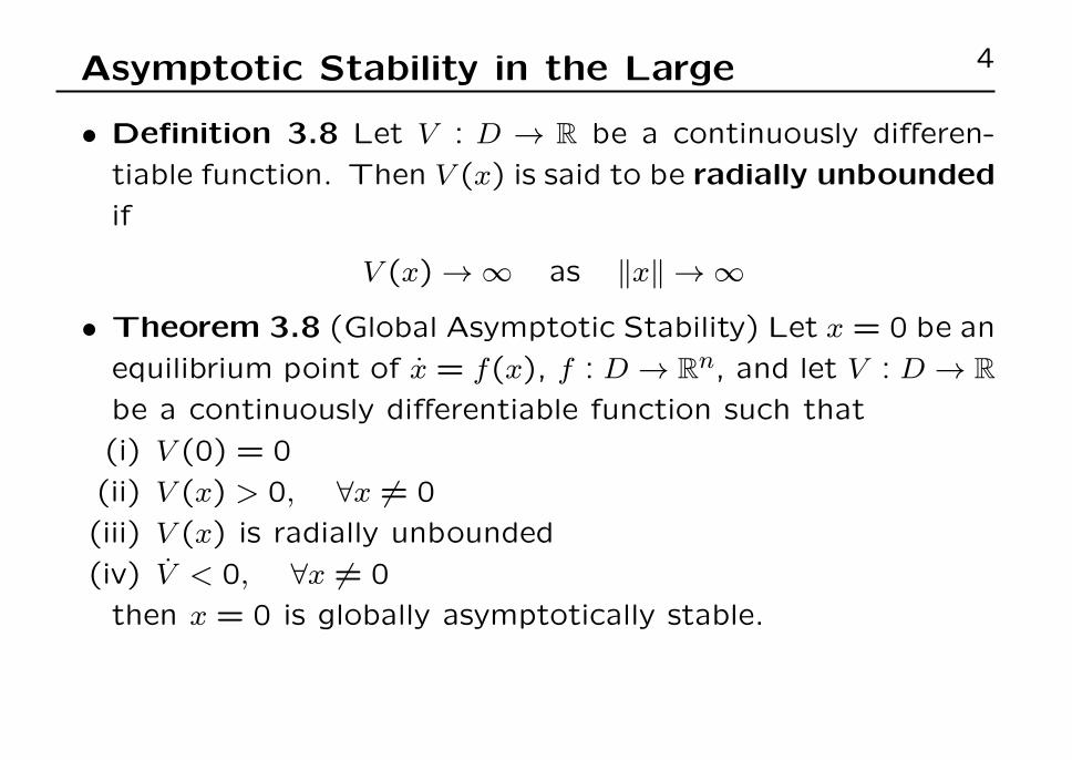
• Definition 3.8 Let V : D → R be a continuously differen-

tiable function. Then V (x) is said to be radially unbounded

if

V (x) → ∞ as ∥x∥ → ∞

• Theorem 3.8 (Global Asymptotic Stability) Let x = 0 be an

equilibrium point of x = f(x), f : D → Rn, and let V : D → Rbe a continuously differentiable function such that

(i) V (0) = 0

(ii) V (x) > 0, ∀x = 0

(iii) V (x) is radially unbounded

(iv) V < 0, ∀x = 0

then x = 0 is globally asymptotically stable.

Example 5

x1 = x2 − x1(x21 + x22)

x2 = −x1 − x2(x21 + x22)

-5 0 5-4

-3

-2

-1

0

1

2

3

4

-1 -0.5 0 0.5 1-1

-0.8

-0.6

-0.4

-0.2

0

0.2

0.4

0.6

0.8

1

(3,0), (0,−3), (0.2,0), (0,−2)

Example 6

• Consider the following system

x1 = x2 − x1(x21 + x22)

x2 = −x1 − x2(x21 + x22)

• To study the equilibrium point at the origin, we define

V (x) = x21 + x22. Then we have

V (x) =∂V

∂xf(x)

= 2[x1, x2][x2 − x1(x21 + x22),−x1 − x2(x

21 + x22)]

T

= −2(x21 + x22)2.

• Thus, V (x) > 0 and V < 0 for all x. Moreover, since V

is radially unbounded, it follows that the origin is globally

asymptotically stable.

Analysis of Linear Time-Invariant Systems

Stability of LTI System 8

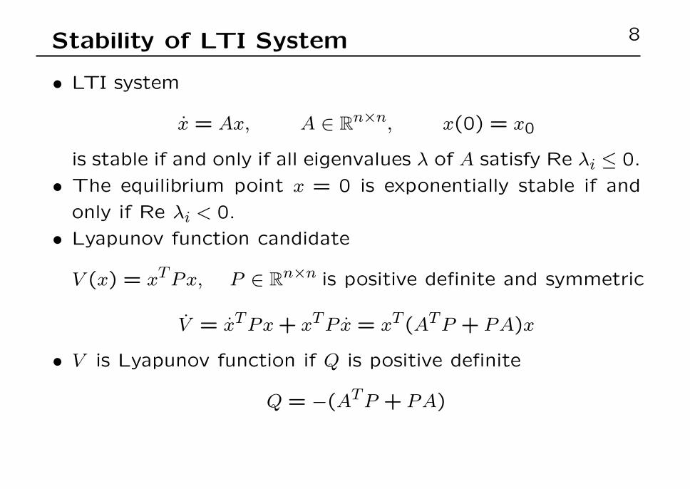
• LTI system

x = Ax, A ∈ Rn×n, x(0) = x0

is stable if and only if all eigenvalues λ of A satisfy Re λi ≤ 0.

• The equilibrium point x = 0 is exponentially stable if and

only if Re λi < 0.

• Lyapunov function candidate

V (x) = xTPx, P ∈ Rn×n is positive definite and symmetric

V = xTPx+ xTP x = xT (ATP + PA)x

• V is Lyapunov function if Q is positive definite

Q = −(ATP + PA)

Stability Check 9

(i) Choose an arbitrary symmetric, positive definite matrix Q.

(ii) Find P that satisfies Q = −(ATP +PA) and verify that P is

positive definite.

• Theorem 3.10 The eigenvalues λi of a matrix A satisfy

Re λi < 0 if and only if for any given symmetric posi-

tive definite matrix Q there exists a unique positive defi-

nite symmetric matrix P satisfying the Lyapunov equation

Q = −(ATP + PA).

Lyapunov’s indirect method

Linearization of Nonlinear Systems 11

• Consider the nonlinear system

x = f(x), f : D → Rn

and assume that x = xe ∈ D is an equilibrium point.• Taylor series expansion about the equilibrium

f(x) = f(xe) +∂f

∂x

∣∣∣∣x=xe

(x− xe) + h.o.ts

• Neglecting the h.o.ts and recalling f(xe) = 0, we have

f(x) =∂f

∂x

∣∣∣∣x=xe

(x− xe)

• Now defining

x = x− xe, ˙x = x, A =∂f

∂x

∣∣∣∣x=xe

=∂f

∂x

∣∣∣∣x=0

we have ˙x = Ax.

Lyapunov’s Indirect Method 12

• Theorem 3.11 Let x = 0 be an equilibrium point for a

nonlinear system x = f(x). Assume that A is a matrix

obtained by liniarization. Then if the eigenvalues λi of the

matrix A satisfy Re λi < 0, the origin is an exponentially

stable equilibrium point.

Exercises 13

• Consider the following dynamical system:

(a)

{x1 = x2x2 = −x1 + x31 − x2

(b)

{x1 = x2x2 = x1 − 2 tan−1(x1 + x2)

(c)

{x1 = 2

3x2x2 = −x1 + x2(1− 3x21 − 2x22)

(a) Find all of its equilibrium points.(b) Find the linear approximation about each equilibrium point,

find the eigenvalues of the resulting A matrix and classifythe stability of each equilibrium point.

(c) Construct the phase portrait of each nonlinear systemand discuss the qualitative behavior of the system.

(d) Construct the phase portrait of the linearized approxima-tions. Discuss the “accuracy” of the approximations.

Feedback Systems

Feedback Systems 15

• Consider the system

x = f(x, u)

and assume that the origin x = 0 is an equilibrium point of

the unforced system x = f(x,0).

• Suppose that input u is obtained using a state feedback

u = ϕ(x).

• Substituting u into x yields a unforced system

x = f(x, ϕ(x))

Feedback Linearization 16

• Example 5.1 Consider the first order system

x = ax2 + u

Is this system stable?

• We look for a state feedback u = ϕ(x) that make the equi-

librium point at the origin “asymptotically stabe.”

• An obvious way is to cancels the nonlinear term

u = −ax2 − x

to obtain

x = −x

which is linear and grobally asymptotically stable.


• It is based on exact cancellation of the nonlinear term ax2.

• This is undesirable since in practice system parameters such

as a are never known exactly.

• Even if the parameters are not exact, the system can be

stabilized.

• But the stability is local because of the presence of the term

(a− a)x2, where a is the true value and a is the actual value

used in the feedback law.

• Cancelling “all” nonlinear terms may not be a good idea

because the nonlinearities are not necessarily bad.


• Example 5.2 Consider the system given by

x = ax2 − x3 + u

and exact cancellation law is

u = u1 = −ax2 + x3 − x

which leads to

x = −x.


• The presence of terms of the form xi with i even (偶数の i) on a dynamical equation is never desirable. Indeed,even powers of x do not discriminate sign of the variable x

and thus have a destabilizing effect that should be avoidedwhenever possible.

• Terms of the form −xj with j odd (奇数の j), on the otherhand, greatly contribute to the feedback law by providingadditional damping for large values of x and are usually ben-eficial.

• At the same time, notice that the cancellation of the termx3 was achieved by incorporating the term x3 in the feed-back law. The presence of this term in u can lead to verylarge values of the input. In practice it may cause actuatorsaturation. The presence of the term x3 on the input u isnot desirable.

Design of Feedback Law

Design of Feedback Law 21

• Given the system

x = f(x, u), x ∈ Rn, u ∈ R, f(0,0) = 0

we proceed to find a feedback law of the form

u = ϕ(x)

such that the feedback system

x = f(x, ϕ(x))

has an asymptotically stable equilibrium at the origin.

Design Policy 22

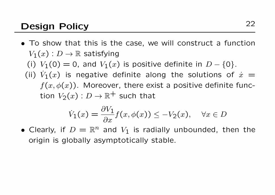
• To show that this is the case, we will construct a function

V1(x) : D → R satisfying

(i) V1(0) = 0, and V1(x) is positive definite in D − {0}.(ii) V1(x) is negative definite along the solutions of x =

f(x, ϕ(x)). Moreover, there exist a positive definite func-

tion V2(x) : D → R+ such that

V1(x) =∂V1∂x

f(x, ϕ(x)) ≤ −V2(x), ∀x ∈ D

• Clearly, if D = Rn and V1 is radially unbounded, then the

origin is globally asymptotically stable.

Example 23

• Consider again the system

x = ax2 − x3 + u

• Define V1(x) = 12x

2 and compute V to obtain

V1 = x · f(x, u) = ax3 − x4 + xu.

• In the previous example we chose u = u1 = −ax2 + x3 − x.

• In this case, we have

V1 = −x2 = −V2(x)

and requirement (ii) above is satisfied.

Example 24

• When we are not happy with the previous example, we mod-ify the function V2 as follows

V1 = ax3 − x4 + xu ≤ −V2(x) = −(x4 + x2)

• In this case we must have

ax3 − x4 + xu ≤ −(x4 + x2)

xu ≤ −x2 − ax3 = −x(x+ ax2)

• The above condition is accomplished by choosing

u = −ax2 − x.

• With this input function u, we obtain

x = ax2 − x3 + u = −x− x3

which is asymptotically stable. The result is global since V1is radially unbounded and D = R.

Backstepping

Integrator Backstepping 26

• Consider a system

x = f(x) + g(x)ξ

ξ = u.

Here x ∈ Rn, ξ ∈ R and [x, ξ]T ∈ Rn+1

• The function u ∈ R is the control input and the functionsf, g : D → Rn are assumed to be smooth.

• It has a cascade connection structure.

-u ∫

-ξ

g(x) -+i -

∫ rx -

�f(·)

6+

Assumptions 27

• Assumptions

(i) The function f satisfies f(0) = 0. Thus the origin is an

equilibrium point of the subsystem x = f(x).

(ii) The first subsystem can be stabilized by a state feedback

ξ = ϕ(x).

• Condition (ii) is actually as follows. We assume that there

exists a state feedback control law of the form

ξ = ϕ(x), ϕ(0) = 0

and a Lyapunov function V1 : D → R+ such that

V1(x) =∂V1∂x

[f(x) + g(x)ϕ(x)] ≤ −Va(x) ≤ 0 ∀x ∈ D

where Va : D → R+ is a positive semidefinite function in D.

Backstepping 28

• An equivalent system

x = f(x) + g(x)ϕ(x) + g(x)(ξ − ϕ(x))

ξ = u.

-u ∫

-ξ +i

−ϕ(x)

6+- g(x) -

+i -

∫ rx -

�f(·) + g(·)ϕ(·)

6+

Backstepping 29

• Define

z = ξ − ϕ(x)

z = ξ − ϕ(x) = u− ϕ(x)

where

ϕ =∂ϕ

∂xx =

∂ϕ

∂xx (f(x) + g(x)ξ)

• This change of variables can be seen as backstepping −ϕ(x)through the integrator.

-u+i

−ϕ(x)

6+-

∫-

zg(x) -

+i -

∫ rx -

�f(·) + g(·)ϕ(·)

6+

Equivalent System 30

• Defining v = z the resulting system is

x = f(x) + g(x)ϕ(x) + g(x)z

z = v.

(i) The system is equivalent to the previous system.(ii) The system is the cascade connection of two subsys-

tems. However it incorporates the stabilizing state feed-bacd ϕ(·) and is asymptotically stable when the input iszero.

-v = z ∫

-z

g(x) -+i -

∫ rx -

�f(·) + g(·)ϕ(·)

6+

Stabilization 31

• To stabilize the system

x = f(x) + g(x)ϕ(x) + g(x)z

z = v

consider a Lyapunov function candidete of the form

V = V (x, ξ) = V1(x) +1

2z2.

We have

V =∂V1∂x

(f(x) + g(x)ϕ(x) + g(x)z) + zz

=∂V1∂x

f(x) +∂V1∂x

g(x)ϕ(x) +∂V1∂x

g(x)z + zv.

Stabilization 32

• We can choose

v = −(∂V1∂x

g(x) + kz

), k > 0

• Thus

V =∂V1∂x

f(x) +∂V1∂x

g(x)ϕ(x)− kz2

=∂V1∂x

(f(x) + g(x)ϕ(x))− kz2

≤ −Va(x)− kz2

• Now we can conclude that x = 0, z = 0 is asymptotically

stable.

• Moreover, since z = ξ − ϕ(x) and ϕ(0) = 0 by assumption,

the origin of the original system x = 0, ξ = 0 is also asymp-

totically stable.

Stabilization 33

• If all the conditions hold globally and V1 is radially un-

bounded, then the origin is globally asymptotically stable.

Documents

System Control Engineering