Embed Size (px)
Citation preview
University of Bath
PHD
A parallel computer based study of the automatic control of power generation
Stagg, T. A.
Award date:1992
Awarding institution:University of Bath
Link to publication
Alternative formatsIf you require this document in an alternative format, please contact:[email protected]
Copyright of this thesis rests with the author. Access is subject to the above licence, if given. If no licence is specified above,original content in this thesis is licensed under the terms of the Creative Commons Attribution-NonCommercial 4.0International (CC BY-NC-ND 4.0) Licence (https://creativecommons.org/licenses/by-nc-nd/4.0/). Any third-party copyrightmaterial present remains the property of its respective owner(s) and is licensed under its existing terms.
Take down policyIf you consider content within Bath's Research Portal to be in breach of UK law, please contact: [email protected] with the details.Your claim will be investigated and, where appropriate, the item will be removed from public view as soon as possible.
Download date: 14. Jan. 2022
A PARALLEL COMPUTER BASED STUDY OF THE
AUTOMATIC CONTROL OF POWER GENERATION
Submitted by T.A.Stagg, B.Sc.(Hons) for the degree of
Doctor of Philosophy of the University of Bath
1992
COPYRIGHT
A ttention is drawn to the fact th a t copyright of this thesis rests with its author. This copy of the thesis has been supplied on condition tha t anyone who consults it is understood to recognise th a t its copyright rests with its author and no information derived from it may be published without the prior w ritten consent of the author.
This thesis may be made available for consultation within the University library and may be photocopied or lent to other libraries for the purposes of consultation.

UMI Number: U042310
All rights reserved
INFORMATION TO ALL USERS The quality of this reproduction is dependent upon the quality of the copy submitted.
In the unlikely event that the author did not send a complete manuscript and there are missing pages, these will be noted. Also, if material had to be removed,
a note will indicate the deletion.
Dissertation Publishing
UMI U042310Published by ProQuest LLC 2014. Copyright in the Dissertation held by the Author.
Microform Edition © ProQuest LLC.All rights reserved. This work is protected against
unauthorized copying under Title 17, United States Code.
ProQuest LLC 789 East Eisenhower Parkway
P.O. Box 1346 Ann Arbor, Ml 48106-1346

< S2X3VER3ITY OF BATHLIBRARY
'2 7 NOV 1992
i ' ¥ H-D
“ S « • > C“
Summary
This thesis describes a potential Autom atic Generation Control (AGC) scheme
for the British power system. The proposal is made to operate the complete
grid as two individual control areas, namely, Scotland and England/W ales. It
is dem onstrated tha t this would allow not only for centralised frequency control
within each area, but also regulation of the power transfer on the tie-lines linking
the two areas. It is also shown how a modification to the Area Control Error
(ACE) would also allow the autom atic control of tim e error and inadvertent en
ergy interchange between the two areas. Current load-frequency control practice
in B ritain is described together with general AGC algorithms and some interna
tional examples of autom atic load-frequency controllers. Research leading to the
development of a simulation set up to study the use of AGC on the British sys
tem is described, together with details of the models involved. These simulation
studies dem onstrate the feasibility of this approach and illustrate improvements
which are possible.
The simulations were executed on a Transputer based parallel com puter using new
parallel processing algorithms. As a result of these simulation studies, guidelines
are given for setting the various param eters and gains of the control system.

Acknowledgements
The author would like to thank Mr A R Daniels, Project Supervisor, for continued
support throughout the course of this work and Prof J F Eastham , Head of School,
for the provision of facilities which enabled the work to be carried out. I would
also like to thank Dr R W Dunn for technical discussions, Mr V S G ott and
Mr B Ross for assistance with the computing facilities, and Mr K W Chan and
other colleagues for parallel developments which were helpful to this project.
Thanks are also due to Mr B M urray of the National Grid Company, Industrial
Supervisor, for the initial idea for this project and support for it, and Mr C Arkell
for technical discussions and supply of information.
The supply of model and controller details from Mr D A Briggs and Dr R Clarke
of Nuclear Electric is gratefully acknowledged.
Finally, I would like to thank Dr R W Dunn once again for proof-reading and
continued encouragement in this endeavour.
This work was carried out under a SERC1 CASE2 award supported by the Na
tional Grid Company, Pic.
This document was prepared using DTjrX.
1 Science and Engineering Research Council2 Co-operative Award in Science and Engineering
C ontents
1 Introduction 1
1.1 Harnessing E n e r g y .................................................................................... 1
1.2 B irth of the Electricity Supply In d u s try ............................................... 2
1.3 Autom ation of Power System C o n tro l.................................................... 4
1.4 About this T h e s is ......................................................................................... 5
2 Control of the British N ational Grid 7
2.1 In tro d u c tio n ................................................................................................. 7
2.2 Current P r a c t i c e ....................................................................................... 10
2.3 S u m m a r y ..................................................................................................... 12
3 A utom atic G eneration Control 14
3.1 In tro d u c tio n ................................................................................................. 14
3.2 The Basic A lg o r ith m ................................................................................ 15
3.3 A History of the Development of A G C ................................................. 16
3.4 Some International Examples of A G C ................................................... 29
3.4.1 The Hungarian S y s te m ................................................................. 29
3.4.2 Electricite de F r a n c e ..................................................................... 32
iii
3.4.3 The Spanish Peninsular S y s te m ............................................... 36
3.4.4 Im atran Voima Oy, F i n l a n d ...................................................... 38
3.4.5 Tacoma City Light Division, U S A ............................................ 41
3.4.6 The Hellenic S y s t e m ................................................................... 43
3.5 Application to the British S y s te m .......................................................... 45
3.5.1 In tro d u c tio n .................................................................................... 45
3.5.2 Previous Experiments ................................................................ 45
3.5.3 Proposal for the A utom atic Generation Control of the BritishNational G r i d ................................................................................. 49
3.6 Summary ...................................................................................................... 49
4 Power System Sim ulation 51
4.1 The Requirement for S im u la tio n s .......................................................... 51
4.2 Simulation of the British National G r id ................................................ 52
4.3 Real Time Power System Simulation at the University of B ath . . 53
4.3.1 In tro d u c tio n .................................................................................... 53
4.3.2 Developments Required for Autom atic Generation ControlS tu d ie s .............................................................................................. 54
4.4 Primemover M o d els ..................................................................................... 56
4.4.1 The Existing Primemover M o d e ls ........................................... 57
4.4.2 New Fossil-Fired Boiler M o d e l.................................................. 57
4.4.3 New Hydro Model ...................................................................... 58
4.4.4 Simulation of the M o d els ............................................................ 59
4.4.5 Load Models ................................................................................ 61
4.4.6 Running the S im u la to r ................................................................ 64
iv
4.4.7 C ontrollers.................................................................................... 67
4.5 S u m m a r y ....................................................................................................... 71
5 C om puting Facilities 73
5.1 Off-Line F ac ilitie s ........................................................................................ 73
5.2 On-Line F a c ilitie s ........................................................................................ 74
5.2.1 H a r d w a r e .................................................................................... 74
5.2.2 S o ftw are ....................................................................................... 78
5.3 S u m m a r y ...................................................................................................... 81
6 Four M achine Studies 82
6.1 Validation of Fossil M o d e l ........................................................................ 82
6.1.1 Stored Energy Tests ..................................................................... 82
6.1.2 Generating Unit Load/Pressure Control T e s t s ................ 83
6.2 Validation of Hydro M o d e l........................................................................ 86
6.2.1 Lookup Tables for Non-Linear C h a ra c te r is tic s ................ 87
6.2.2 Response to Manual Ramping of Guide Vane Position . . . 87
6.2.3 Response to Power Setpoint Change ....................................... 87
6.3 System Split S tu d i e s .................................................................................. 88
6.3.1 System with Dinorwig Generating and Insensitive Loads . 89
6.3.2 System with Dinorwig Pumping and Insensitive Loads . . 92
6.3.3 Longer Timescale R esp o n ses .................................................. 95
6.3.4 Systems with Frequency and Voltage Dependent Loads . . 96
6.3.5 Power/Frequency Characteristics C a lc u la tio n s ................ 97
6.4 Step Load Change S tu d ie s ........................................................................ 98
v
6.4.1 Tests w ith D istributed Frequency R egu la tion ................ 99
6.4.2 Tests with Centralised Autom atic Generation Controllers . 105
6.4.3 The Effect of the AGC Frequency Bias Param eter B . . . 106
6.4.4 The Effect of AGC Controller Gains Tn and Cp ......................109
6.4.5 A New Area Control E r r o r .............................................................. I l l
6.4.6 The Effect of Controller In te rv a l.................................................... 112
6.4.7 Effects of System Operating C ond itions.......................................115
6.5 S u m m a r y ......................................................................................................... 117
7 Tw enty-Five M achine Studies 120
7.1 System Split T e s t ............................................................................................120
7.2 Step Load Change S tu d ie s ...........................................................................123
7.2.1 More Effective R e g u la t io n .............................................................. 124
7.2.2 The Effect of Different Setpoint Rate L im i t s .................... 125
7.2.3 The Use of Low Frequency Relays on Hydro P la n t ........... 126
8 Conclusions 128
9 Further Work 135
A ppendices 138
A Fossil-Fired Boiler M odel R outine Listings 138
B Fossil-Fired Boiler M odel Variables 140
C Fossil-Fired Boiler M odel Equations 143
vi
D Pum ped-Storage M odel Variables 146
E Pum ped-Storage M odel Equations 149
F Four Equivalent M achine Study Files 154
F .l M aster F i l e .................................................................................................... 154
F.2 Busbar and Line D a t a ................................................................................ 155
F.3 Primemover D a t a .......................................................................................... 156
F.4 Generator and AVR D a t a ......................................................................... 157
F.5 Adm ittance M atrix Ordering D ata ........................................................ 158
G Tw enty-Five Equivalent M achine Study Files 159
G .l M aster F i l e .................................................................................................... 159
G.2 Primemover D a t a .......................................................................................... 160
G.3 Generator D a t a ..............................................................................................162
G.4 Generator Group D a t a ................................................................................164
G.5 Busbar and Line D a t a ................................................................................167
G.6 A dm ittance M atrix Reordering D a t a .....................................................174
G.7 Load D a t a ........................................................................................................176
H B F T Pressure Loop Controller D esign 179
I B F T Load Loop Controller Design 191
J Conversion of Fossil M odel for Coal and for 660 M W U nits 200
J . l Creation of Coal-Fired M o d e l .................................................................. 200
J.2 Creation of 660 MW Unit M o d e l...............................................................200
vii
K D ig itis a tio n o f C o n tro lle rs 206
K .l S y m b o ls ............................................................................................................ 206
K.2 Integral C o n t r o l le r ........................................................................................207
K.3 Proportional-Integral C o n tro lle r ................................................................ 208
L D e ta ils o f F o u r M ac h in e S im u la tio n R u n s 209
M D e ta ils o f T w e n ty -F iv e M ac h in e S im u la tio n R u n s 218
F ig u re s 220
B ib lio g ra p h y 387
viii
Symbols and Abbreviations
ACE Area Control Error
ACEN New Area Control Error
AFRC Area Frequency Response Characteristic
AGC A utom atic Generation Control
ASC Area Supplementary Control
a Integral gain in ACEN
BFT Boiler Follows Turbine
B Frequency Bias Param eter
Area Droop or AFRC
CASO Computer Assisted System Operation
CED Constrained Economic Dispatch
CEGB Central Electricity Generating Board
CRT Cathode Ray Tube
DMA Direct Memory Access
DRAM Dynamic Random Access Memory
EACC Error Adaptive Control Computer
ED Economic Dispatch
EDF Electricite de France
ELD Economic Load Dispatch
A / System frequency error

GOAL Generator Ordering and Loading
GT Gas Turbine
I Integral only Control
IBM Trademark, International BusinessMachines, Inc.
II Inadvertent Interchange
10 In p u t/O u tpu t
I VO Im atran Voima Oy, Finland
K{ Integral Controller Gain
K p Proportional Controller Gain
LFC Load Frequency Control
NAPSIC North American Power SystemsInterconnection Committee
NCC National Control Centre
O PF Optim al Power Flow
PC Personal Computer
PD P Trademark, Digital Equipment Corporation
PI Proportional-Integral Control
A Pt N ett tie-line power imbalance
RAM Random Access Memory
ROM Read Only Memory
Pi Participation factor of i th generator
x
SCADA Supervisory Control and D ata Acquisition
SD Security Dispatch
SED Secure Economic Dispatch
ss Steady State
SSEB South of Scotland Electricity Board
TD Time Deviation
TFB Turbine Follows Boiler
VAX Trademark, Digital Equipment Corporation
VDU Visual Display Unit
VLSI Very Large Scale Integration
VSC Video and System Controller
Symbols relating to primemover model variables and param eters are given
appendices B-E.
List o f Figures
2.1 Typical Daily Load C u r v e .........................................................................220
4.1 Schematic of Simulator Model S t r u c t u r e ................................................ 221
4.2 Schematic of Original General Governor M o d el...................................... 221
4.3 Fossil-Fired boiler sch e m a tic ..................................................................... 222
4.4 Schematic of Dinorwig Pum ped Storage S c h e m e ................................ 223
4.5a The British SuperGrid S y s te m ............................................................... 224a
4.5b Equivalent Four Machine N etw ork ........................................................ 224b
4.5c Equivalent Twenty-Five Machine N e tw o r k ....................................... 224c
4.6 Typical Boiler Follows Turbine s t r u c tu r e ................................................ 225
4.7 Typical Turbine Follows Boiler s t r u c tu r e ................................................226
4.8 Block Diagram of Fossil-Fired Boiler Model ....................................... 227
4.9 Block Diagram of BFT Pressure Loop PI C o n t r o l ............................... 228
4.10 Block Diagram of BFT Load Loop I C o n tro l ......................................... 228
5.1 Block Diagram of the Parallel Transputer C o m p u te r............................ 229
5.2 Block Diagram of the Inmos T800 T r a n s p u te r ...................................... 229
5.3 Block Diagram of the T800 Processing N o d e ......................................... 230
5.4 Block Diagram of the 10 B o a r d ................................................................. 231
5.5 Block Diagram of the Graphics B o a rd ..................................................... 232
xii
5.6 Block Diagram of Transputer Network C o n fig u ra tio n .........................233
6.1 4 m ’c NWALES Stored Energy Test 400 MW (Run 4 7 c ) .................234
6.2 4 m ’c NWALES Stored Energy Test 400 MW (Run 4 8 c ) .................235
6.3 4 m ’c NWALES Stored Energy Test 400 MW (Run 4 9 c ) .................236
6.4 4 m ’c NWALES and CEGB Load Setpoint Changes (Run 43) . . 237
6.5 4 m ’c NWALES and CEGB Load Setpoint Changes (Run 45) . . 239
6.6 4 m ’c NWALES Pressure Setpoint Change (Run 4 2 ) ....................... 241
6.7 4 m ’c NWALES Pressure Setpoint Change (Run 4 4 ) ....................... 243
6.8 DINORWIG Non-Linear Characteristics ................................................ 245
6.9 4 m ’c DINORWIG Manual Guide Vane Ramp (Run 5 1 ) .....................246
6.10 4 m ’c DINORWIG Response to Step Load Increase (Run 52) . . . 247
6.11 4 m ’c Scotland-England Split (Run 1 ) ..........................................248
6.12 4 m ’c Scotland-England Split (Run 2 ) ..........................................250
6.13 4 m ’c Scotland-England Split (Run 3 ) ..........................................252
6.14 4 m ’c Scotland-England Split (Run 4 ) ..........................................254
6.15 4 m ’c Scotland-England Split (Run 5 ) ..........................................256
6.16 4 m ’c Scotland-England Split (Run 6 ) ..........................................258
6.17 4 m ’c Scotland-England Split (Run 7 ) ..........................................260
6.18 4 m ’c Scotland-England Split (Run 8 ) .......................................... 262
6.19 4 m ’c Scotland-England Split (Run 5 a ) .......................................264
6.20 4 m ’c Scotland-England Split (Run 6 a ) .......................................266
6.21 4 m ’c Scotland-England Split (Run 2 1 ) .......................................268
6.22 4 m ’c Scotland-England Split (Run 6 1 ) .......................................270
xiii
6.23 4 m ’c Step Load Increase busbar CEGB4 (Run 9 ) ..............................272
6.24 4 m ’c Step Load Increase busbar CEGB4 (Run 10) 274
6.25 4 m ’c Step Load Increase busbar CEGB4 (Run 11) 276
6.26 4 m ’c Step Load Increase busbar CEGB4 (Run 12) .......................... 278
6.27 4 m ’c Step Load Increase busbar CEGB4 (Run 13) 280
6.28 4 m ’c SCOTLAND Ldv 4- 500 MW CEGB -5 0 0 MW (Run 14) . . 282
6.29 4 m ’c SCOTLAND Ldv + 500 MW CEGB -5 0 0 MW (Run 15) . . 284
6.30 4 m ’c Step Load Increase busbar CEGB4 (Run 16) 286
6.31 4 m ’c Step Load Increase busbar CEGB4 (Run 18) ..........................288
6.32 4 m ’c Step Load Increase busbar CEGB4 (Run 19) ..........................290
6.33 4 m ’c Step Load Increase busbar CEGB4 (Run 19) ..........................292
6.34 4 m ’c Step Load Increase busbar CEGB4 (Run 20) 294
6.35 4 m ’c Step Load Increase busbar CEGB4 (Run 21) 296
6.36 4 m ’c Step Load Increase busbar CEGB4 (Run 1 9 b ) ..........................298
6.37 4 m ’c Step Load Increase busbar CEGB4 (Run 2 0 b ) ..........................300
6.38 4 m ’c Step Load Increase busbar CEGB4 (Run 2 1 b ) ..........................302
6.39 4 m ’c Step Load Increase busbar CEGB4 (Run 2 2 b ) ..........................304
6.40 4 m ’c Step Load Increase busbar CEGB4 (Run 23) 306
6.41 4 m ’c Step Load Increase busbar CEGB4 (Run 24) 308
6.42 4 m ’c Step Load Increase busbar CEGB4 (Run 25) 310
6.43 4 m ’c Step Load Increase busbar CEGB4 (Run 26) 312
6.44 4 m ’c Step Load Increase busbar CEGB4 (Run 27) 314
6.45 4 m ’c Step Load Increase busbar CEGB4 (Run 28) 316
xiv
6.46 4 m ’c Step Load Increase busbar CEGB4 (Run 29) 318
6.47 4 m ’c Step Load Increase busbar CEGB4 (Run 30) 320
6.48 4 m ’c Step Load Increase busbar CEGB4 (Run 32) 322
6.49 4 m ’c Step Load Increase busbar CEGB4 (Run 31) ...........................324
6.50 4 m ’c Step Load Increase busbar CEGB4 (Run 3 6 a ) ...........................326
6.51 4 m ’c Step Load Increase busbar CEGB4 (Run 3 5 a ) ...........................328
6.52 4 m ’c Step Load Increase busbar CEGB4 (Run 33) 330
6.53 4 m ’c Step Load Increase busbar CEGB4 (Run 34) 332
6.54 4 m ’c Step Load Increase busbar CEGB4 (Run 3 6 b ) ...........................334
6.55 4 m ’c Step Load Increase busbar CEGB4 (Run 3 5 b ) ...........................336
6.56 4 m ’c Step Load Increase busbar CEGB4 (Run 2 7 b ) ...........................338
6.57 4 m ’c Step Load Increase busbar CEGB4 (Run 41) 340
6.58 4 m ’c Step Load Increase busbar CEGB4 (Run 40) ....................... 342
7.1 25 m ’c Scotland-England Split (Run 1 ) .................................................. 344
7.2 25 m ’c Step Load Change (Run 1 0 ) ..........................................................348
7.3 25 m ’c Step Load Change (Run 9 ) .............................................................353
7.4 25 m ’c Step Load Change (Run 8 ) .............................................................358
7.5 25 m ’c Step Load Change (Run 7 ) .............................................................363
H .l Block Diagram of P lant in BFT Pressure L o o p .................................... 368
H.2 B FT Pressure Loop Block Diagram T ran sfo rm a tio n .......................... 369
H.3 Block Diagram of Proportional C o n tro l ..................................................372
H.4 Pressure Loop Root Locus with Proportional C o n tr o l ........................372
H.5 Block Diagram of Proportional-Integral C o n t r o l ..................................373
xv
H.6 Root Locus of Pressure Loop with Fast Zero in PI Controller . . . 373
H.7 Root Locus of Pressure Loop with Slow Zero in PI Controller . . . 374
H.8 Root Locus of Pressure Loop with Zero at s = —0 . 0 1 .......................374
H.9 Root Locus of Pressure Loop at 360 MW with Zero at s = —0.01 . 375
I.1 Block Diagram of P lant in B FT Load L o o p ...........................................376
1.2 BFT Load Loop Block Diagram T ran sfo rm atio n .................................377
1.3 Root Locus of Load Loop with Proportional Control @ 170 MW . 381
1.4 Root Locus of Load Loop with Proportional Control @250 MW . 381
1.5 Root Locus of Load Loop with Proportional Control @ 390 MW . 382
1.6 Root Locus of Load Loop with Proportional Control @490 MW . 382
1.7 Block Diagram of Integral C o n tro l........................................................... 383
1.8 Root Locus of Load Loop with Integral Control @170 MW . . . . 384
1.9 Root Locus of Load Loop with Integral Control @ 250 MW . . . . 384
1.10 Root Locus of Load Loop with Integral Control @390 MW . . . . 385
1.11 Root Locus of Load Loop with Integral Control @490 MW . . . . 385
1.12 Root Locus of Load Loop with K i — 0.00025 @390 MW .................386
xvi
C hapter 1
Introduction
But as it might be supposed that in all the preceding experiments of this section, it was by some peculiar effect taking place during the formation of the magnet, and not by its mere virtual approximation, that the momentary induced current was excited, the following experiment was made. All the similar ends of the compound hollow helix were bound together by copper wire, forming two general terminations, and these were connected with the galvanometer. The soft iron cylinder was removed, and a cylindrical magnet, three-quarters of an inch in diameter and eight inches and a half in length, used instead. One end of this magnet was introduced into the axis of the helix, and then, the galvanometer-needle being stationary, the magnet was suddenly thrust in; immediately the needle was deflected in the same direction as if the magnet had been formed by either of the two preceding processes. Being left in, the needle resumed its first position, and then the magnet being withdrawn the needle was deflected in the opposite direction. These effects were not great; but by introducing and withdrawing the magnet, so that the impulse each time should be added to those previously communicated to the needle, the latter could be made to vibrate through an arc of 180° or more.
Michael Faraday, Nov, 1831
1.1 H arn essin g E nergy
Ever since Man first evolved, his abilities and skills in utilising natural sources
of energy have been param ount to his survival and development. Very early on,
he learned to use fire to make his lifestyle both safer and more comfortable. Life
1

was enhanced further by other inventions and discoveries — the bow and arrow
to make hunting easier, the use of horses and other beasts of burden for transport
and driving machinery, the harnessing of water and wind power enabling easier
trade over longer distances and, most recently, the prolific use of fossil fuels which
began with the industrial revolution. Now electricity has become one of the most
im portant forms of energy in the modern world. At its point of use it is clean,
it is readily transported over large distances, it is easily controllable and it is the
only useful way of utilising the potential of some other forms of energy such as
radioactivity.
1.2 B ir th o f th e E lec tr ic ity Su p p ly In d u stry
W ith Michael Faraday’s discovery of electromagnetic induction in 1831, the scene
was set for the development of a world-changing technology. The earlier invention
of the steam engine was to provide the mechanical power for this im portant new
energy conversion process. However, it was to be another forty years before the
industrial generation of electricity became a practical question with Gram m e’s
production of a dynamo with a ring-wound arm ature (the “Gramme Ring”) [1].
This was followed by a rapid increase in the use of electricity which is still contin
uing to accelerate today. The earliest supplies were almost exclusively for street
lighting, initially by arc lamps and then incandescent lamps, patented by Thomas
Edison in 1879. By the end of the century, many other application had developed
including electric railways, electric welding, electric smelting and also a number
of domestic electrical appliances such as flat irons, fans, immersion heaters and
cookers. The induction motor had been invented by Tesla and has formed an
increasing share of the electricity demand. Electric washing machines were intro
duced in the USA in 1907, vacuum cleaners in 1908 and electric refrigerators in
2

1912. Electric refrigerators were first used in Britain in 1918.
The first public supply of electricity in Great Britain was used to light the streets
of Godalming in 1881 using current generated by the waters of the River Wey. The
following year, the first steam power stations for public supply were operational.
The Holborn Viaduct power station, financed by the Edison Electric Light Co. of
London claimed the distinction of being the first public steam power station in the
world to cater for the needs of the private consumer as well as for public lighting.
The Brighton power station was regarded as the first viable public supply station
providing the first perm anent public supply in England to all consumers who
desired it. These first supplies were direct current but the debate was soon to
s tart over whether direct or alternating current should be used. In 1882 Gaulard
and Gibbs obtained British Patents for alternating current distribution by means
of transformers operating in series, and in 1884, Dr John Hopkinson showed
m athem atically tha t alternators could, in fact, by run in parallel, which was later
confirmed by experiments by Prof Grylls Adams. 1884 also saw the construction
by Sir Charles Parsons of the world’s first turbo-generator, a d.c. unit capable of
developing about 75 A at 100 V. In 1888, Parsons supplied the first of four 75 kW
single phase turbo-alternators to the Newcastle and District Electric Lighting Co.
Ltd. — the earliest use of the steam turbine in a public power station.
The London Electric Supply Corporation’s famous Deptford power station —
later to be known as Deptford East — started up in 1889. This was designed by
Ferranti for the transmission of power at 10,000 V a.c. to transformers placed in
the Central London area which reduced the voltage in two steps to 100 V for sup
plying incandescent lamps. The two 1500 hp, 10,000 V alternators operating at
5000 rpm , or 8 3 | Hz, were by far the largest in the world at th a t time. Transmis
sion over the seven miles to Central London was by underground cables designed
3
and m anufactured by Ferranti at the station.
The first overhead transmission lines were erected in Britain in about 1890, and in
1891 the long distance power transmission by three-phase alternating current was
foreshadowed by experiments by Oskar van Millar in Germany. The first three-
phase public supply in B ritain was installed in 1900 from the Neptune Bank power
station of the Newcastle-upon-Tyne Electric Supply Co. to local shipyards, works
etc. — the first example of bulk supply. Later, in 1903, Parsons supplied this
station with a 2 MW three-phase alternator with a rotating field, a radical change
which has never been abandoned. This was rated at 2 MW, 6000 V, 40 Hz.
By this tim e, the so-called B attle of the Systems had effectively been won by the
proponents of alternating current. Steady progress had been made towards ever
larger machines and higher voltages and this finally dictated the use of a.c. for
transmission, though there were pockets of d.c. still operating in the 1950s. By
1910, steam turbines had become the common form of primemover and power
stations needed only bled steam, feed water heating, steam reheat and higher
initial steam conditions to make them modern [2].
1.3 A u to m a tio n o f P ow er S y stem C ontrol
W ith the recent privatisation of the electricity supply industry in Britain and
the associated separation of responsibilities for generation and transmission into
separate companies, together with a shift of emphasis towards operation under
commercial contracts, there has been renewed interest in the autom atic control of
the power system. The new commercial environment may well provide incentives
for autom ating grid control where contracts would exist with generating stations
4
for their participation in frequency regulation and load following. Indeed, there
is already a move towards centralised setting of generation targets away from the
traditional inter-area transfer system where several smaller control areas (within
England and Wales) set their own targets for regulation.
The proposal of this thesis is to operate the complete British power system as
two individual control areas, namely, Scotland and England/W ales. Autom atic
Generation Control (AGC) would be applied in each of these areas allowing both
system frequency and power transfer between the two areas to be controlled. A
simulation has been developed which is suitable for the study of this mode of
operation. Results taken from this simulation have allowed suggestions to be
made with regard to the setting of various controller param eters and gains.
1.4 A b ou t th is T h esis
C hapter 2 presents the development of control of the British power system. The
current practice is described and the effect of privatisation on future developments
is discussed.
General AGC algorithms are presented in chapter 3. This is followed by some
international examples of centralised Load-Frequency Control (LFC). Previous
experiments of autom atic LFC on the British system are discussed together with
potential future developments.
Simulations are discussed in chapter 4. Development of power system simulation
at the University of Bath is presented and the modifications necessary for the
current study are described. Details are given for models of different primemover
5
types and loads, and generating unit control is discussed.
C hapter 5 gives details of the computing facilities available for this work. Several
types of hardware and software were used in both the off-line and on-line aspects
of this work. The main engine for the complex simulation work was a Transputer
based parallel com puter details of which are given in this chapter.
The main results of the simulation work are presented in chapter 6. This de
scribes a series of experiments designed to enable decisions to be made regarding
controller param eters and gains. The chapter ends by detailing proposals for the
autom atic load-frequency control of the British power grid.
Some supplem entary results are discussed in chapter 7. These were obtained
using a more complex model of the grid network than those of chapter 6 and
dem onstrate some characteristics arising from the non-uniformity of generator
types which exist in a real system.
Conclusions and suggestions for further work are given in chapters 8 and 9 re
spectively.
6

C hapter 2
Control o f the B ritish N ational Grid
2.1 In trod u ction
The electricity supply industry of the early 20th century was made up of a large
number of independent power companies and municipal undertakings. In 1926
the Central Electricity Board was set up by the Electricity (Supply) Act to con
centrate generation in a num ber of selected stations and to interconnect these to
the existing regional system by a national ‘G rid’. By the outbreak of war in 1939,
interconnection between the districts was commonplace and the national system
was normally operated as one interconnected system with a national control cen
tre in London and six district control centres [3].
Essentially, the purpose of grid control is to meet the demand for electric power
as economically as possible subject to the constraints of security of supply and
plant availability and performance. The system has always been controlled m an
ually by operators in a hierarchical organisation: national control - area control -
plant control, though increasing off-line computer assistance has been available.
7
The problem is solved in two phases—an off-line one referred to as operational
planning, which includes scheduling of generation, and an on-line one called load
dispatching. Scheduling defines in advance the generators th a t will be connected
to the system at any tim e and proposes tim e for their connection and disconnec
tion, whereas dispatching allocates loads to them in accordance with the criteria
of economy and security [4]. Between dispatches instructed by the Grid Control
Area control engineers, the balance of generation to demand is m aintained by the
speed governors of those generators able to respond to system frequency changes.
The main stream developments in grid control over the last th irty years has
been the introduction of increasingly powerful computer tools to aid the control
engineer. Throughout the 1960s a comprehensive suite of programs was built
up [5, 6]. Load flow programs enabled calculations to be made of power flows
in each line of a large system and of the resulting flows in the event of circuit
outages, fault levels and losses. Demand was predicted using previous demand
patterns and allowing for weather. A comprehensive optim isation program fed
with data on costs, on plant availability and constraints and on the configuration
of the transmission system, calculated the optim um schedule th a t determined
the start-up and shut-down of m ajor units, the required area im ports/exports
and provided the specified spare. A term inal gave the control engineers access to
the computer. In 1970 a new national control centre was commissioned, equipped
with comprehensive computer-driven displays and an on-line security assessor [6].
By the early 1980s com putational facilities for operational planning work were
provided by the CASO (Com puter Assisted System Operation) network, which
consisted of a network of seven communications processors, five sited a t Regional
Headquarters or Grid Control Centres, and two at the CEGB’s Computing Cen
tre in London. One of these was dedicated to National Control use and the other
8
provided a general support and standby service for the other six. The proces
sors were connected radially to the Board’s Central Com puter installation by
British Telecom circuits (9.6 kbaud) and also to the Regional main computers
as appropriate. Some one hundred VDUs were connected to the system and in
stalled in control rooms and operational planning offices. The system provided
facilities for transmission of data between any processors on the system, namely,
Regional main-frame processors, the communications processors and the Head
quarters Control Centre installation. The original CASO system was later re
placed because of obsolescence by a system of colour VDUs using high-definition
displays.
1984 saw the introduction into full-time service of the GOAL (Generator Or
dering and Loading) program which had been extensively tested and developed
operationally since early 1981 [7]. The previous m anual system was based on
the use of incremental production costs alone and it was recognised tha t a more
rigorous approach was necessary to take account of tim e dependent factors, prin
cipally start-up costs, in the optimisation. Improvements were realised in peak
period plant selection, management of plant over low demand periods, scheduling
pum ped storage in the most economic m anner, representing the effects of dual
firing and better modelling of the effect of transmission constraints. The GOAL
program was also incorporated in the long term planning suite, where it is used
to derive annual heat requirements. The associated fuel supply program then
derives optim um fuel allocations and associated heat costs.
In addition to the developments in grid control, there have been parallel improve
ments in the control and performance of the power plants [3, 8, 9, 10, 11, 12, 13,
14]. In the main, these have aimed towards the following, at times contradictory,
requirements: increased efficiency, increased flexibility to grid requirements eg.
9
run-up times and frequency regulation ability, reduced wear and tear, improved
environmental im pact etc.
2.2 C urrent P ra ctice
A few statistics describing the size [15] of the British power supply system are as
follows:
Net Capability 53954 MWMaximum demand m et (86/87) 47925 MWAnnual Energy Sales 228 TW hNumber of Power Stations 74
Plant mix: Number Net Capability ProductionMW % TW h %
Coal 36 30886 57.2 186.4 81.7Oil 5 8417 15.6 9.3 4.1Gas Turbine 11 1302 2.4 - -
Coal/O il 3 4504 8.3 - -Coal/Gas 1 366 0.7 - -Nuclear 10 5069 9.4 32.8 14.4Pum ped Storage 2 2088 3.9 0.659 0.3Hydro 6 107 0.2 0.249 0.2O ther (eg Auxiliary GTs) - 1215 2.25 0.026 0.01Total 74 53954 100.0 228.1 100.0External (eg. ED F1, SSEB2) - 2000+ 16.524
The load curve for a typical weekday is shown in figure 2.1.
Under the current manual operation of the system, the National Control Centre
directs each of five Area Control Centres to m aintain a defined im port or export
1Electricite de France2South of Scotland Electricity Board
10
of power until a new instruction is given. This is known as the Inter-Area Transfer
system [16]. The power transfers are calculated off-line in advance and updated
using the best available information and each u n it’s costs and constraints and
the capability of the transmission system. The targets can be biased by the Area
Control Centres in proportion to system frequency error, to reinforce the effect
of governor action and the load/frequency controllers operating in some plant.
In addition to this form of frequency control, several units at the Dinorwig hydro
station may be kept on Low Frequency Relay start such th a t they will cut in at
m aximum generation should a serious fall in frequency occur.
Studies into generation and transmission requirements will be carried out by the
planning departm ent up to five or ten years ahead. Operational control of the
grid system starts about six weeks ahead of the event with the use of DC and
AC load flow studies together with predicted demand profiles to produce detailed
generation schedules minimising operating costs whilst taking into account the
known generation and transmission constraints and allowing sufficient margins
for contingencies. As the lead tim e decreases and more current information be
comes available, better estim ates can be made of demand, generation and network
conditions and the frequency of studies is increased. Estim ates of conditions are
m ade daily for the following day, and throughout the day, some eight times a
day, for conditions four hours ahead. Extensive use is made of the GOAL pro
gram [7] in the production of the generation schedules and loading programme to
minimise costs given generation and transmission constraints. S tate estimation
is performed on metered data to ensure consistency before being used by other
programs or stored in historical databanks for use in future load prediction stud
ies. Load flow programs are used to ensure th a t current and proposed operating
conditions allow acceptable power flows under normal and outage conditions, and
also acceptable fault levels under contingencies.
11
Control of the grid requires the metering of a large amount of data. The Grid
Control Centres acquire da ta from the power stations and substations, much
of which is also transm itted on to National Control, generally via lines hired
from British Telecom. The data includes items such as the status (open/closed)
of all circuit-breakers and autom atic isolators, active and reactive power flows,
voltages, frequencies from several points. The frequency of da ta telem etry ensures
th a t between three and five values for each item are received every m inute [17].
These data are asynchronous and are not tim e-stam ped until received by the
control centre computers where they are integrated over one and th irty minute
periods to reduce measurement noise and to synchronise to a common time.
Post-privatisation, some aspects of grid control are changing. The Inter Area
Transfer system is to be superceded by a system whereby to tal Area Generation
Targets are to be sent from national to area control centres instead of area trans
fers. This move towards centralised dispatching of area targets will be accom
panied by the further development of frequency corrections being set nationally
instead of by the separate areas as has happened in the past. This centralising of
generation dispatching would lead nicely into the form of autom atic generation
control discussed later in this thesis.
2.3 Sum m ary
This chapter has described the mode of operation of the control of the national
grid. Early history, development and current practice have been described to
gether with some operational changes arising from the privatisation of the elec
tricity supply industry. It would appear th a t current developments are leading
towards a more centralised control of system frequency which could well be en-
12

hanced by the proposals in this thesis. The next chapter describes some aspects
of centralised load-frequency control and autom atic generation control.
13
C hapter 3
A utom atic G eneration Control
3.1 In trod u ction
There is some discrepancy within the literature as to the exact meaning of the
term Autom atic Generation Control, or AGC. Some authors consider it to be
simply a new name for Load Frequency Control (LFC) [18] although others feel
tha t it covers a wider range of functions [19]. Most recent works have used the
term to describe the control function which autom atically matches power gen
eration to demand whilst minimising costs. W hether the system is autom atic
or manual, this is generally done in a two stage manner. An economic opti
misation is performed to determ ine the optimal m anner in which the required
generation should be shared amongst the generators (Economic Dispatch, ED).
At a much faster rate, Load Frequency Control is performed whereby generation
is m atched to demand by regulating the system frequency and power interchange
with neighbouring utilities. The manner in which this regulation is performed
will be described in this chapter together with a description of some authors’ pro
posals to improve the basic algorithm whilst taking better account of economy
and security.
14
3.2 T h e B asic A lgorith m
Centralised load-frequency control, LFC, is used extensively in interconnected
power systems such as those of continental Europe and the USA. Each area
within the system forms its own Area Control Error, ACE, based on the errors in
frequency and im ported/exported tie-line powers. For many years now, tie-line
bias control has been used where,
AC E = A P t + B A f
A P t is the imbalance between scheduled and actual tie-line real power, measured
positive out of the area, and A f is the imbalance between scheduled and actual
frequency. B is the frequency bias param eter relating frequency to power. Nor
mally, B is set equal to the effective area droop or Area Frequency Response
Characteristic, AFRC, as it is often called by American utilities. The AFRC is
measured in M W /Hz and in the literature is generally denoted by the symbols
K or /?. The AFRC can be measured on a given system or area by noting the
frequency change for a particular load change [20]. The AFRC, also known as
the power/frequency characteristic, depends very much on the prevailing gener
ation and loading conditions. Reference [20] derives an equation for estim ating
the power/frequency characteristic of the British Grid system of the 1950s from
a knowledge of the turbine capacity on the busbars and the system load.
The Area Control Error is used by the controller to calculate a change of genera
tion required to bring the ACE back to zero. In general, European utilities use a
proportional-integral, PI, controller, whereas American utilities employ integral,
I, only control. In these cases the required change in generation can be calculated
from the ACE as:
15
( K p AC E + K i jA C E d t for PI controlA U —
( Ki J AC E dt for I control
K p and K{ are controller gains.
The required generation is shared amongst the n participating generators in pro
portions denoted by their participation factors, pi, where,
n
^ 2 Pi = 1 i = 1,2, . . . n1 = 1
The participation factors may be calculated off-line, or on-line by the economic
dispatch program running at less frequent intervals than load-frequency control.
How much of the supplem entary generation each generator will be expected to
supply will depend on such factors as economy and the speed of response of the
generator.
3.3 A H isto ry o f th e D evelop m en t o f A G C
The basic ideas of tie-line bias control were formulated in the 1930s when the
earliest European interconnections were made [21]. At this time, the so-called
Graner-Darrieus condition of non-intervention was formulated [22, 23] whereby
the frequency bias, B , is made equal to the effective droop of the area. W ith this
setting, a load change in one area does not result in a steady state change in the
power exported to it by its neighbours.
By the late 1950s, load-frequency control based on these principles was well es
tablished in the European system [24]. deQuervain and Frey in [24] outlined a
16
num ber of different configurations connecting separate power systems and means
of controlling frequency and tie-line powers. They also discussed the design and
operation of a digital electronic controller to replace the electro-mechanical types
th a t had previously been in use for many years. They felt th a t the definite and
contractual schedule of power interchange between systems and groups of systems
was the very backbone of power economics and th a t, in this case, load-frequency
control, based on system frequency and tie-line power, was essential.
In the mid 1960s, Quazza formalised a general approach to the linear analysis and
synthesis of the stiff-interconnection n-area electric power system control [25]. In
such a situation, the tie-line power exchanges between each of the n areas was
to be controlled together with the system frequency, assumed equal in all areas
due to the “stiff” nature of the system. Two approaches to the design of load-
frequency controllers were suggested, both of which ensured the basic advantage
of splitting the n-dimensional problem into n one-dimensional problems. The
first approach required non-interaction between the frequency and tie-line pow
ers controls and the second required th a t each controlled area took care of its own
load variations. The second criterion closely reflected the then current, and sub
sequent, practice with the sound advantage tha t each local area controller could
be synthesised simply on the basis of its own area transfer function, without any
need to know the transfer functions of the other areas. The first criterion required
th a t all control loops had the same transfer functions, which Quazza considered
definitely preferable. No real advantage was seen, however, in the non-interaction
between frequency and exported power control.
At a similar time, Ross defined the LFC problem as the need to minimize area
control error (ACE), inadvertent interchange (II), and tim e deviation (TD) with
a minimum of area supplem entary control (ASC) activity [26]. He proposed
17

an error adaptive control computer, EACC, which, in effect, monitored the error
signal and calculated the probability th a t control action was required. The EACC
considered the error signal, ACE, to consist of three components — deterministic,
probabilistic and sustained. The first two were assumed to be rapidly varying
fluctuations for which no effective control action was possible or desired. Field
tests and simulation studies showed a remarkable reduction in control activity
with no significant increase in ACE.
A 1970 paper by Elgerd and Fosha [27] questioned the North American Power
Systems Interconnection Com m ittee’s (NAPSIC) recommendation tha t each con
trol area set its frequency bias equal to the area frequency response characteristic
(AFRC), a practice also followed by European utilities. They presented what
they considered to be a set of typical minimum requirements of the controller:
1. The static frequency error following a step-load change must be zero.
2. The transient frequency swings should not exceed ± 0.02 Hz under normal
conditions.
3. The static change in the tie-line power flow following a step-load change in
either area must be zero.
4. The tim e error should not exceed ± 3 seconds.
5. The individual generators within each area should divide their loads for
optim um economy.
The authors presented the development of a ninth-order linear perturbation
model of a two-area power system. An analog com puter was used to simulate
this system and to calculate a cost function based on the integral of the squares
18
of tie-line power and frequency deviations. These results enabled the authors to
propose values for the frequency bias setting and the value of the gain of the
typical American integral controller.
Using this model, Fosha and Elgerd went on to develop a full state feedback opti
mal controller for the two-area power system [28]. In this case, a load-frequency
controller was developed for each area which took account of all the model states
— ie. even those from the other area. By noting the relatively small size of the
gains associated with states from the other area, these states were ignored for the
local controller. Consequently, a controller for each area was developed which
used only states from its own area. The authors dem onstrated the improvement
over using the conventional controller possible when more system information
was fed back.
This series of two papers, [27, 28], provoked a lot of discussion, much of which was
concerned with the lack of detail in the models used, particularly with regard to
governor non-linearities and generator rate limits. It was pointed out by several
discussers th a t the simulated results presented were totally unrealistic because of
the slow effects th a t had been ignored. Consequently, the changes to established
operating practice recommended could not be taken seriously. However, the
application of new control techniques to load-frequency control was welcomed.
Glavitsch and Galiana proposed separating system conditions and disturbances
into classes with an appropriate control strategy associated with each class [29].
The proposed classes and strategies were:
I: < 2% in base area — requires maintenance of a smooth control signal. The
system should be able to follow trends in the load.
19
I I A: < 5% base area — limited control action should be used to keep frequency
and tie-line power deviations as small as possible and returned to zero
within a reasonable time.
I IB : < 5% other areas — similar to IIA with the base area being led to support
the troubled area.
I l l : > 5% — spinning reserve m ust be allocated such th a t the expected operating
cost is a minimum for a given risk of failure.
It was suggested th a t Kalman filtering techniques should be used to detect the
different disturbance classes. The authors developed a simplified linear model
which took account of the m ajor dynamics of a power system fed by coal fired
plant and the uncertainties associated with modelling some parts of the system
— particularly the interconnected areas outside of the base area. The proposed
control scheme included a state estim ator based upon this model to account
for uncertain and unmeasurable quantities. Optim al state-feedback controllers
(continuous) were designed off-line for each of the disturbance classes I, IIA and
IIB to be applied to the system on detection of the appropriate class. A relatively
detailed, non-linear model was used to compare the proposed control scheme with
current operating practice. Gains were quoted for conventional LFC of Cp = 0.1-
1.0 and Tn = 10-30 seconds, where,
u(t) = Cp AC E + ^ - jA C E d t (3.1)J-n J
A model addressing many of the shortcomings of tha t in [27] is tha t of deMello,
Mills and B ’Rells presented in [30]. This is a model of one control area tied to a
very large interconnected power system. The linear model was able to represent
the principal dynamics significant for A utom atic Generation Control studies. The
20
simulation included a num ber of sub-systems modelling the electro-mechanical
plant, the prim emover/energy supply system including boiler effects and pressure
controls, load reference actuation representing the digital raise/lower pulse logic
used to change the turbine load reference, and load disturbance models composed
of several components including fairly slow ramps, rapidly changing “noise” , and
occasional step changes due to, for example, the disconnection of generators.
A companion paper to [30] described techniques for the application of autom atic
digital generation control and for the evaluation of performance indices which
measured the effectiveness of control relative to the control effort [31]. The pro
posed performance indices included the standard deviation of Area Control Error,
the integral of Area Control Error and a measure of the control effort taken as
the accumulation of control pulses without regard to sign. In order to prevent
unnecessary control action and to not allow the relatively slow generating units
to chase high frequency variations in the ACE, the authors proposed non-linear
digital filtering in the unit controllers whereby control action would be prevented,
or lim ited, until a sufficient error had been accumulated. Further logic could be
included in the AGC to disallow control action if the ACE were already in a
direction to reduce the integral of ACE, yet not so large as to warrant immedi
ate control action. Simulation results were presented using the model developed
in [30]. The paper addressed some of the significant practical concerns of AGC
and the authors reflected th a t logic and intuitive thinking were invaluable in the
design of a control system. However, they also cautioned against the adoption of
unnecessarily complex control structures which are relatively easy to implement
in software. They further warned against the dangers of using inadequate models
with the consequent development of impracticable control strategies.
At the end of the 1970s, the principal concerns of power system operators with
21

regard to autom atic generation control were ones of economy of regulation and
quality of regulation — how they might be assessed and how they might be op
timised [32]. Criteria for regulation performance in the North American systems
were laid down, and constantly reviewed, by NAPSIC. At this tim e the sort of
conditions specified for control performance were quoted as:
A l . The Area Control Error must equal zero at least one tim e in all ten-m inute
periods.
A 2. The average ACE for all ten-m inute periods must be within a specified limit
th a t is determined from the area’s rate of change of load characteristic.
B l . For disturbance conditions, the ACE must be returned to zero w ithin ten
minutes.
B 2. Corrective action m ust be forthcoming within one minute following a dis
turbance.
Surveys were carried out amongst member utilities to determine compliance with
the criteria.
In 1980 a review paper appeared which presented an overview of current operating
practice and also the problems which were emerging as power systems continued
to develop [18]. The paper outlined the tried and tested technique of tie-line
bias control and quotes typical gains for equation 3.1 of Cp = 0.1-0.3 and Tn =
30-100 seconds. Comparing these figures with those given in 1972 [29] (quoted on
page 20) reflects the decrease in speed of load-frequency control over this period.
There were a number of contributing factors for this, not least of which were
the increased proportion of coal-fired regulating plant and the replacement of
22
analogue controllers with digital ones with associated sampled measurements as
systems increased in size and complexity. Glavitsch and Stoffel highlighted the in
creasing inadequacies of the conventional control algorithm as systems continued
to become more heavily interconnected and supplied by ever larger generating
units. In a control area connected to other areas with only a few tie-lines, the
net interchange power is a reasonable reflection of the generation-load imbalance
in the area and the area controller is able to modify it. However, when an area
is heavily interconnected with other areas, this is no longer the case as a power
transfer across an area does not appear in the net interchange. Consequently,
tha t area cannot control the power flow on the interconnecting lines. Hence,
there was an increasing interest in schemes th a t allowed individual control of
lines. It was envisaged th a t one such scheme might employ optimal power flow
techniques whereby the AGC requirements might be dynamically shared amongst
generators so as to influence the distribution of power flow.
In the 1980s, studies were aimed at sam pled-data autom atic generation control
using simulations which took account of system non-linearities such as generation
rate constraints and governor dead-band effects. The systems being simulated
also started to become more complex. Discussions ensued amongst researchers
as to the adequacy and validity of some of the models being used.
A 1981 paper by Kothari et al. [33] analysed the effect of generator rate con
straints on load-frequency control of a two-area power system. A discrete power
system model was developed using the same sampling interval as the proposed
controller — 2 seconds. However, the model involved tim e constants much smaller
than this — 0.3 and 0.08 seconds. On modelling a 1% step load perturbation
and varying the sampling interval from 0.1 seconds to 1.5 seconds, the results
showed increasing instability and loss of higher frequency effects. From this,
23
the authors concluded th a t the given controller gain was not suitable for use at
higher controller intervals rather than questioning whether the model was still
adequate or even valid at the higher modelling interval. Consequently, the results
are questionable and the conclusions unproven. This point was taken up by other
researchers in this area and a correspondence appeared in IEE proceedings [34].
The same basic model was used by Tripathy et al. in [35] and it is not at all
clear th a t it was not being used in the same invalid way. This paper presented
a m ethod of determining optim um gains by minimizing a cost function by the
discrete Lyapunov technique, which, unlike as in [33], appeared not to require
repeated simulation runs. However, it did use the discrete version of the model
with a sampling period given as T . Since the controller gains and states are
augmented with the discrete model of the plant, it is not obvious how, if at all,
the controller and plant can be modelled with different tim e intervals. However,
the m ethod of using optim al control to choose “best” controller gains was clearly
illustrated and the model did a ttem pt to include the very real effects of some
system non-linearities.
A further analysis using simulation including representation of governor deadband
and minimisation of cost functions to both dem onstrate the deteriorating effect
of such non-linearities and to present a methodology for choosing controller gains
was presented by Basanez and Riera [36]. These authors dismissed the widely
accepted model of Elgerd [27] and used a more complete model based on tha t
proposed by Davison [37] into which governor non-linearities had been incorpo
rated. This model represented a rather more complex power system than what
was considered to be the rather trivial two equal-area models used extensively in
the past. It would appear from [36] th a t a discrete model had not been considered
in this case.
24

Kum ar et al. proposed using a discrete variable structure controller whereby the
control action is either integral or proportional depending on the m agnitude of
the ACE [38]. The authors commenced by taking pains, once again, to stress the
im portance of adhering to Shannon’s sampling theorem when digitising models.
However, here a differential, not difference, model was used. The analysis was
based on a four-area interconnected system with a m ixture of reheat therm al,
non-reheat therm al and hydro units. The unit models also incorporated governor
deadband models as used in [35], together with generator ra te limits.
Another development which came to be more seriously considered in the 1980s
for use in Autom atic Generation Control was the use of Optim al Power Flow
(O PF) techniques [39]. A 1988 paper by Bacher and Van Meeteren described
the concept, m athem atical formulation and solution of a real-tim e optim al power
flow in an Energy M anagement System. Traditionally, a full O PF, often referred
to as Security Dispatch (SD), uses a S tate Estim ator solution as a base case
and reschedules generation whenever a branch overload occurs. An SD execution
interval of th irty minutes is typical. New upper or lower unit limits resulting from
SD are provided to Economic Dispatch (ED) which shares the to tal generation
optimally (in an economic sense) between units as constrained by these limits.
Bacher and Van Meeteren highlighted some disadvantages of this approach:
“Between two consecutive SD calculations the state of the power
system will vary and therefore, the dispatch as provided by ED will
not be optim al and secure over this period.
LFC unit mode changes and unit lim it changes may result in
branch flow violations th a t cannot be controlled until SD is executed
again.
Many unit base points may be set at either their new upper or
25
lower limit, resulting in a participation factor of zero. This means
th a t fewer units are available to pick up a change in required system
generation.”
In the proposed approach, Economic Dispatch is replaced by Constrained Eco
nomic Dispatch (CED). S tate Estim ator output is used in SD to identify over
loaded branches or other violated network flow constraints. Using linear program
ming techniques, a critical constraint set is then identified by optimising the State
Estim ator base case subject to network flow constraints. The critical constraint
set is used by CED to optimise generation using quadratic programming tech
niques to determ ine optim al and secure LFC participation factors. CED would
typically run every three minutes, although during periods of rapid load change
execution may be initiated every th irty seconds.
M .L.Kothari et al. proposed a new area control error (ACEN) based on tie-power
deviation, frequency deviation, tim e error and inadvertent interchange [40]. A
controller using this error always guarantees zero steady state time error and
inadvertent interchange, unlike conventional ACE controllers. Based on simula
tion studies, the authors found th a t the settling tim e for tie-power and frequency
deviations was more with the new ACE controller. However, conventional ACE
controllers require supplem entary control whereby offsets are made in scheduled
frequency and area net interchange to correct for accumulated errors.
The proposed new Area Control Error is given by:
ACEN = APtie + B A f + ae 4- c tl
where
26
* = 505a
e = tim e error
I = inadvertent interchange
a, a = constants
ACEN may alternatively be expressed as:
AC E N = (A PUe + B A f ) + a J (A P ,ie + B A f ) dt
ie.
ACEN = AC E + a J A C E dt (3.2)
Unfortunately, this analysis was based upon the same model as th a t previously
used in [33] where both the controller and power system were discretised at the
controller interval of two seconds. Consequently, the quantitative results are
questionable and the use of this model was again questioned in the discussion of
[40]. However, the proposal to use a new ACE based upon conventional ACE and
integral of conventional ACE appears to be one worth persuing for the additional
benefits of autom atic correction of tim e error and inadvertent energy interchange.
Come the end of the 1980s, North American utilities were still very much con
cerned with the cost of A utom atic Generation Control, inadvertent energy inter
change and tim e error [41]. Apart from the initial installation and ongoing m ain
tenance costs, AGC imposes an economic burden on day to day operations. The
system operator must consider the startup and running costs of a unit equipped
with AGC versus one without. A number of cost factors come into play when
AGC is considered, eg., efficiency losses, uneconomic loading of units while try
ing to satisfy the ACE, wear and tear on units under autom atic control and lost
27
sales due to low frequency operation. If one utility has customers connected to
someone else’s system, th a t utility must compare the costs of buying regulation
to support th a t load with the cost of appropriate telem etry to take their load
into account in its own AGC. Poor regulation and /or inadequate dispatch of
generation lead to further costs through inadvertent energy and tim e error and
the ensuing correction procedures. There is a feeling amongst medium to large
American utilities (10,000-25,000 MW) th a t AGC costs alone are in the millions
of dollars per year.
Two very recent papers seem to have fallen into the trap of using very sophis
ticated control techniques, but inadequate models leading to unrealistic control
schemes inappropriate for operational use.
The design of a multivariable self-tuning regulator for a load frequency control
system with the inclusion of interaction of voltage on load demand has been
presented by Yamashita and Miyagi [42]. The analysis has been performed on a
two-area model. The controller inputs are the area frequency deviation and the
tie-line power deviation. The controller outputs are commanded changes in speed
changer position and excitation voltage. A controller interval of 0.5 seconds was
chosen, which is rather faster than the frequently quoted telemetering interval of
two seconds for many utilities. The simulation used in the analysis only models
non-reheat turbines and consequently does not take account of the slower modern
therm al units, neither does it consider plant non-linearities such as generator ra te
constraints. Having modelled the effect of voltage deviation on load demand, the
analysis does not take account of any voltage regulation would would also be
a ttem pting to alter the excitation voltage in order to keep the term inal voltage
constant.
28
Aldeen and Marsh have presented a decentralised design m ethod for LFC of a
two-area power system in which each area is able to estim ate the states of the
whole system [43]. The analysis uses the model of Elgerd and Fosha and the
authors seem to have totally mistaken the comments given in the discussion of
th a t paper: [27]. Consequently, the final results are unrealistic, being able to
return the frequency deviation on a step load change to zero steady state within
five seconds. Many modern operational controllers are of the sam pled-data type
with a control interval of five seconds or more. However, it is very interesting to
note th a t the to tal state vector of the two-area system is observable from each
individual area. The authors state their intention to analyse more complex area
interconnections to see if this approach is extendable to more realistic systems.
3 .4 Som e In tern ation a l E xam p les o f A G C
Further to the examples detailed below, an interesting survey of the application
of a standard AGC package to a number of different power systems, varying in
both size and structure are to be found in reference [44].
3.4.1 T he Hungarian System
The Hungarian power system consists of 750 kV, 400 kV, 220 kV and 120 kV net
works with perm anent interconnections with neighbouring countries a t all levels
[45, 46]. The system is mainly therm al based w ith very little hydro generation,
w ith an average load of 3400 MW, and an area droop of about 350 M W /H z. More
than 20% of energy consumption is imported.
29

The control objectives for a new AGC in Hungary were set out as follows:
• The area should regulate its own load fluctuations.
• It should contribute to the control of system frequency.
• During the accounting intervals, the exported or im ported energy should
be of scheduled value.
• The regulator should satisfy the requirement at minimum cost.
• The regulator should reduce the commands sent to the power stations w ith
out compromising other control objectives.
Some of these objectives were contradictory, hence an optim al controller was
used which implemented a compromise. AGC was realised in two levels: load-
frequency control (LFC) and economic load dispatch (ELD). LFC and ELD have
been integrated into a single AGC such th a t LFC is done with regard to generation
economics.
In 1979, a load-frequency controller was installed which could adapt to the avail
ability of controllable units [45]. Because the control was performed only by
means of slow-acting therm al power plants, it was assumed the dynamic be
haviour of the plants could be characterised mainly by their rate of change of
generation.
The LFC used a typical Area Control Error:
AC E = (Pt - P0) - B ( f - f 0)
with the convention th a t positive ACE required an increase in generation and
th a t Pt was positive for power flow into the area. P0 and f 0 are setpoint values.
30
An adaptive integral controller was designed whereby
Gi = C, j A C E d t
such th a t Gd = desired generation change
r> — mL' 1 ~ ACE
M = rate of change of generation
The command sent to each unit was the to tal desired generation made up of the
economical setpoint and some portion of Gd-
Gci = Gbi + piGd
where, Gd = command to be sent to the ith plant
Gbi = economic setpoint
Pi = participation factor
It was found from simulation studies tha t if there were great differences in the
rates of change of generation of the controlled plants, this algorithm did not give
the expected optim al results because the participation factors were evaluated on
the basis of economics and not on the rates. Consequently, Gd had to be modified
to take this into account.
This controller proved to be inconvenient because of the high control effort needed
and the requirement to encompass a special half-an-hour accounting system work
ing on the base of the integral of the area control error.
A digital controller was designed which took account of the delay tim e of the
process and output control signals based on predicted load conditions [46]. An
autoregressive moving average process was used for modelling the load distur
bance. Unneccessary control effort was avoided by limiting the control signal
31

when the area control error was not too large.
Using filtered values of signals measured every two seconds, the controller op
erated every minute. Measurements included tie-line powers, system frequency,
generation of individual power plants and the num ber of controllable units within
a plant. This was in contrast to the first scheme which operated every two sec
onds. The second controller was installed in June 1881.
3.4.2 E lectricite de France
In recent years Electricite de France, EDF, have been pursuing a m ajor project
to replace their grid control system. A new real-tim e com puter system for the
national control centre was installed in 1982 and provided: SCADA, LFC, state
estim ation, security analysis, open-loop secure economic dispatch, power schedule
updating, and optim al power flow applications. A longer term project is secure
autom atic generation control using more powerful computers. The French system
is one of the largest in the world to be operated by a single utility — about a
quarter as large again as the British National Grid. M ajor statistics for 1984/85
were [47, 48]:
Total Demand 282 TW hTotal Generation 309 TW hPeak G eneration1 60,000 MWNuclear 60%Fossil 20%Hydro 20%
EDF provides about 90% of this energy, owns and operates the transmission
network and most of the distribution network. There are forty nuclear and fossil
1 January 1985
32

stations consisting 120 units between 125-1300 MW and 500 hydro plants of
which fifty are im portant. The transmission network is made up of 14,000 km
of 400 kV lines, 25,000 km of 225 kV lines, 3000 circuits, 1500 transformers and
about th irty links with foreign countries. This is operated through one national
and seven regional control centres. The regional centres are mainly concerned
w ith distribution and some ‘regional’ hydro plants. Currently, only LFC orders
are sent directly to the plants by the National Control Centre, all other power
changes being carried out through the regional centres.
The National Control Centre directly controls:
• the whole 400 kV network = 70 substations
• 100 225 kV substations
• 40 substations representing foreign networks near borders
• 230 generating units for which active and reactive power is transm itted to
NCC. This includes all units connected at 400 kV and the main units at
225 kV.
The network size handled by NCC is 200-300 nodes, whereas taking the whole
225 kV network would lead to a network between 600-700 nodes.
Scheduling is done on two mainframes — an IBM 3033 and a 3081, located
at the Research Division with terminals at the control centres. The new real
tim e com puter system of NCC is built around two M ITRA 525 mini-computers
(0.3 M IPS2) with 16-bit words, linked to a data network by two SOLAR 16/40
2on a scale where a VAX 11/780 = 1.1 MIPS
33
front-end computers (0.1 MIPS) operating in a redundant configuration. There
are fourteen full graphic four-colour CRTs with a resolution of 2048x2048 pixels
w ith a light pen, track ball and keyboard interface. Two pictures are needed to
display the whole of the 400 kV network of seventy substations showing nodes
and line flows. An anim ated mimic board has been kept as a back-up. 2200
telemeasurem ents and 5500 telesignals are scanned every ten seconds while switch
positions are transm itted only on a change or on call.
3 .4 .2 .1 In te g ra l L F C
The current method of Load Frequency Control is very conventional. The ACE
(for all of France) is integrated and multiplied by a convenient factor at the
national control centre, then sent to all the plants (single control order, the same
for all plants). Frequency is measured every second, tie-line powers every two
seconds. The controller interval is ten seconds.
3.4 .2 .2 Secure A utom atic G eneration Control
An on-going long term development of EDF is secure autom atic generation control
which will enable Load Frequency Control and Secure Economic Dispatch to be
perform ed together at the current LFC rate of ten seconds [19, 48, 49]. Initial
studies were started on the project in 1981 with the agreement to go ahead with
it being made in 1985. The latest estim ate is for installation in 1995 [19].
The input signals to the closed loop SED control law are the ACE and the bind
ing security constraints. The outputs are the generating unit power setpoints. It
34
was found necessary to partition the required load changes into two components
— a trend component and an oscillatory component. The oscillatory component
is range limited and has zero mean. It is shared proportionally amongst all par
ticipating generators as for conventional LFC. This has been called ‘secondary
control’ and can be justified because such small amplitude, short duration distur
bances have very small consequences with regard to economy and security. The
trend component is used by the secure economic dispatch together with the criti
cal constraints to calculate secure and economic generations for all units. This is
known as ‘tertiary control’. W ithout this partitioning, the SED would cause the
small oscillatory component of the load to be chased by only a few generating
units causing undesirable wear and tear. The filter used in the partitioning was
made to be adaptive so th a t for increasing magnitudes of load disturbances, the
tertiary control took more responsibility and the secondary less. In this way,
large load changes which would have significant consequences on economy and
security are reacted to by the tertiary control in a fast manner.
The operating intervals of the various functions making up the secure autom atic
generation control will be as follows:
• Frequency will be measured every second.
• Tie-line powers will be measured every two seconds (synchronised and time-
stam ped).
• Every ten th second SCADA will be carried out on the 400kV /225kV net
works to include about 1000 busses. Critical constraints and AGC outputs
are calculated.
• S tate estim ation will be performed every minute as well as AGC supervisory
control which checks controller performance and, when necessary, adjusts
35
the param eters of the control system.
• Global and bus load forecasts will be carried out every fifth minute, pro
ducing forecasts for five and twenty minutes ahead and providing an active
reduced model to be used by AGC.
• Security analysis will be performed every fifteenth minute, and on call, for a
few hours ahead using active/reactive optim al power flows, also producing
forecasts for five and twenty minutes ahead.
A num ber of simulation models have been developed in order to test, improve
and validate the new AGC system. Both simple and very detailed models are
being used to further develop the controller in an iterative process of design
and simulation testing [49]. A first version of a large simulation model with
explicit network modelling has now been set up. The simulation consists of three
m ain subsystems modelling the power system, the data transmission system and
the central control system. The power system subsystem models the full French
400 kV and 225 kV networks and equivalent networks for Western Europe totalling
1050 nodes. Long term primemover dynamics are represented in detail including
control and computer functions at the plants.
3.4.3 T he Spanish Peninsular System
The Spanish system is made up off several heavily interconnected utilities [50].
The m ajor statistics a t the end of 1983 were:
400 kV lines: 9,140 km 220 kV lines: 15,070 km
to tal area: 505,000 km 24 tie-lines with France
36
Installed capacity: 36,514 MW Hydro: 14,003 MW
Conventional Thermal: 17,668 MWNuclear: 4,843 MW
Total demand: 98,080 MWhPeak load: 18,630 MW
A shared regulating system was put into operation in the first quarter of 1983,
with seven areas participating. The utilities responsible for load frequency control
did not cover the whole power system and consequently, the regulating pool mem
bers had to compensate for their non-regulating partners. A hierarchical control
scheme was employed whereby the national control centre calculated a to ta l pool
regulating requirement based on the net interchange deviation with France and
shared this amongst the participating areas. Each area had its own Autom atic
Generation Control which regulated its own area net interchange deviation as
well as system frequency and the to tal pool regulating requirement.
At the national level, the Pool Regulating Requirement, PER, was calculated as:
A
PER = G x FPNID - Y NIDit = 0
where G is the Pool gain, FPNID is the Filtered Pool Net Interchange Deviation,
NID{ the regulating area Net Interchange Deviations and A the number of active
regulating areas. PER was shared amongst the pool members according to partic
ipation factors, PFi, to produce individual Company Regulating Requirements,
e m u
A
CRRi = PER x PFi Y PF' = 1t = 0
37
The AGC algorithm then used by each area was as follows:
ACEi = NIDi - B i A f + CBRi
On disconnection from France, each AC E took account only of frequency, ie.
ACEi = - B i A f
The Pool Control Function was executed every eight seconds.
3.4.4 Im atran Voim a Oy, Finland
Im atran Voima Oy, IVO, is the state owned utility supplying 40-45% of the
annual electricity sales in Finland [51, 52]. In 1985 IVO supplied 22.7 TW h of
electricity made up of supplies from its own plants, power purchased from other
Finnish power companies and imports from the USSR and Sweden. The share of
generation in Finland is divided as follows:
40-45% IVO + other state owned companies 40% industrial producers 15% municipal utilities
Total IVO capacity is 4900 MW made up of:
1400 MW hydro 1200 MW nuclear 1700 MW other therm al 600 MW com m itted imports
links to Sweden: 2x400kV -f lx 2 2 0 k V lineslinks to USSR: 1000 MW dc link
38
In 1984 the to tal Finnish production was 47.1 TW h plus 4 TW h im ported from
the USSR.
IVO owns all of the 400 kV grid, most of the 220 kV grid and about a half of the
110 kV grid.
A joint operation agreement exists between Denmark, Finland, Norway and Swe
den which deals with, among other things, tem porary transactions between p art
ners, generation and voltage control and maintenance of production reserves.
The IVO System Control Centre is regarded as a National Control Centre. A new
Control Centre System was commissioned in 1981 in which data received a t the
National Control Centre from District Centres included about 700 measurements
plus 2100 status indications from the power system control and 500 other data
items from separated and centralised control system supervisory equipment. This
was transm itted via IVO’s own radio link and power line carriers. D ata trans
mission for the centralised AGC was carried out by connections separate from
the D istrict Centre Systems.
The control system at the National Control Centre consisted of a Front-End com
puter system made up of three PD P 11/34 computers (two, in a redundant mode,
for da ta transmission and one for telesupervisory and software maintenance use)
and a Main com puter system. The main computer system consisted of two 16-bit
Modcomp Classic mini-computers (in redundant configuration). There were four
consoles and monitors in the control centre and remote terminals in the district
centres and large power plants. These remote terminals were used to display
production plans and for entering manual data tha t could not be measured, such
as generator availability, tem porary limitations, control characteristics and fuel
39
costs.
Load forecasts were performed off-line on VAX 11/785 computers and on-line
in the control centre systems. This was done from one hour ahead to one week
ahead with hourly mean values corrected for tem perature. Tem perature is signif
icant in Finland because of the high domestic heating load (10% of the country’s
consumption). Effects of tem porary contracts for selling and purchasing energy
were estim ated and entered manually.
Dispatched setpoints were sent to control centres and power plant control rooms
but were acted on manually, whereas AGC requirements were sent direct to the
plant.
The inputs to the A utom atic Generation Control were the tie-line power on the
links with Sweden and the system frequency. The outputs were the desired out
puts from two hydro power plant groups and the dc link with the USSR giving a
to ta l of 1200 MW. There were four different operating modes. The normal mode
was an hourly energy balance control:
AC E = A P + B A f
/•1 /ir
U = A C E d t Jo
In tie-line power control AC E = A P , though this is rarely used. W hen A f >
0.3 Hz, or the interconnection with Sweden is out of service, frequency control
mode is employed where AC E = B A f . The final mode is m anual control where
only the turbine governors control frequency.
40

These algorithms were performed by a digital com puter in the Central Control
Centre, but there were analogue back-up controllers in two of the district centres.
The central controller sent the control signals to the group controllers which in
tu rn shared it between their own power plants, adding the new signal to the
current setpoint values and sending the new setpoints to the local controllers.
The local controller distributed the signal to the turbine governors, keeping the
turbine powers equal.
A P was calculated by dedicated equipment in one district centre using load
measurements of the tie-lines and the setpoint value. It was then sent to the
central controller. Frequency was measured at a 400 kV substation and sent
to the central controller which calculated the frequency deviation. The central
controller was a PD P 11/34. The AGC application programs were w ritten in-
house.
This control centre system was fully operational in 1982. The software was main
tained in-house, though it was supplied by an independent supplier. Preliminary
studies were started in 1973 and all deliverables were finally accepted in 1983,
three years late. This was due mainly to the under-estim ation of what was in
volved and difficulties in preparing completely unambiguous specifications.
3.4.5 Tacom a C ity Light D ivision, U SA
This is another example of regulating hydro turbines [53]. The company has six
hydro generating plants (eighteen generators) with a to tal capacity of 760 MW
in an area whose load is 1100 MW. The area is interconnected to the North West
Power Pool via six inter-ties. The communications between the energy control
41
centre and the generating sites is done via dedicated microwave links. Other
rem ote terminals are connected by microwave or telephone lines. Tie-line real
power, line frequency and generator power outputs are each measured at two
second intervals.
The AGC algorithm in this case is based upon an Area Control Error calculated
from:
AC E = Y , Pt(i) ~P * + 10B ( f — f , ) + TC
where
m = Power flow in tie-line i, MW
Ps = Net scheduled interchange power, MW
B = Frequency bias setting, MW /O.lHz
f , f s = Actual and scheduled frequencies, Hz
TC = tim e correction, MW, derived from the seconds of tim e error multiplied by a number, M W /sec
The controller interval in this case is eight seconds. This interval was chosen
through operational experience taking into consideration the load and intercon
nection behaviour, governor action and hydro generator response. ACE is com
puted every two seconds and the generator control is executed every eight seconds.
The controller compares the actual generator outputs with their desired values
and sends corrective raise/lower signals to the governors. The basic control loop
was analysed and designed using a transform formulation.
Another significant concern of this system was to consider the allocation of water
usage among the plants.
42
3.4.6 T he H ellenic System
A Load Frequency Control for the Hellenic power system has been proposed [54]
which has three types of LFC: flat frequency, flat tie-line and tie-line bias, and four
operating modes which depend on the m agnitude of the area control error: steady
state, normal, and two emergency modes. An approximate economic dispatch is
suggested which uses a predetermined table of the economic loading of units to
work within the present computer hardware limitations. The full system is to be
implemented on a dual mini-computer system.
The Hellenic power system has been modelled as fourteen power plants — six
therm al, eight hydro — and one tie-line to Yugoslavia and hence the West Euro
pean power pool. The installed capacity is 5566 MW.
The calculation of the Area Control Error is modified according to the type of
LFC:
flat frequency: ACE = B A f
flat tie-line: AC E = A Pt
tie-line bias: AC E = B A f + A P t
The control period is slow — th irty seconds. The authors claim some advan
tages of slow acting LFC: non-interaction with machine dynamics, relative non
sensitivity to changes in the power system also avoids unnecessary excursions
of unit output power due to transient faults. There is no consideration of rate
of change of generation in the controller. The authors also claim th a t the sys
tem characteristic (in M W /Hz) is the only necessary information for the design
of a slow acting LFC system. They use integral of frequency error feedback to
43
correct the cumulative frequency error, to filter measurement errors and the sta
tistical load component, and also because the frequency control system responds
to transient faults to a far lesser extent.
There are six measurement intervals in every control period, ie. the measurement
period is taken as five seconds, each measurement in fact being the average of five
one-second measurements. In this way, filtering of the measurements is achieved
and transient values will not be acted upon by the controller. The control period
is th irty seconds. The comparatively long control interval has been dictated by
the slow communications speeds available on the Hellenic system.
The required change in generation required is calculated from:
n 1A G = p A C E n + (1 - p) V -A C E j
L—/ n3-1
where n is the measuring intervals per control interval. Simulation studies have
found th a t p = .25 is adequate to filter out possible measurement errors without
deteriorating the speed of response.
A com putational algorithm has been developed to evaluate the approxim ate par
ticipation factors of all the generating units participating in the frequency control
scheme from a m atrix containing generator loading information under various
system loading levels. The algorithm is implemented every fifteen minutes.
44
3.5 A p p lica tio n to th e B r itish S y stem
3.5.1 Introduction
Since the formation of the National Grid, the British power system has been
operated as an isolated system by a single utility. It has not had the contractual
obligations to neighbouring utilities as happens on the continent and in America,
for instance, which requires a tight control of tie-line power flows and system fre
quency. Consequently, there has been little progress made towards autom ating
the dispatch/loading function and providing centralised frequency control. How
ever, it may be beneficial to have some form of autom atic generation control even
in an isolated system in th a t it may allow, for example, for a system-wide rather
than a local optim isation to handle short term variations from predictions and
for economic benefits arising from more frequent optimisation [16]. Indeed, there
are a num ber of isolated power systems in the world which have chosen to use
standard AGC software as part of their modernised control systems [55, 56, 57].
3.5.2 Previous Experim ents
Some of the earliest interest in providing autom atic generation control for the
CEGB system was provoked by the examination of the possibility of establishing
an a.c. link between the French and British systems in the early 1950s. This
need disappeared with the decision to use a d.c. cable for technical and economic
reasons. However, some experimental work continued to investigate the feasibility
and requirements of autom atic frequency control for the isolated British system
[20, 58].
45
Two quite m ajor experiments have since been carried out by the CEGB into
autom atic and centralised control of the grid. The first of these took place in
the mid 1960s and was concerned with the autom atic control of a number of
generators in the South West region [59, 60, 61, 62, 63, 64, 65, 6 6 , 67]. The
second was a study of centralised dispatch in the early to mid 1980s [4, 16, 17].
3.5.2.1 The South W est Region AGC Experim ent
A 1960 paper by Casson, Moran and Taylor [6 8 ] foreshadowed the requirement
for the autom atic loading of the generating plant on the CEGB system. A few
years later a limited experimental scheme was set up on part of the CEGB system
in order to clarify the technical and economic issues involved [6 6 , 67]. The field
trials were preceded by a laboratory experiment which was effectively an exercise
in autom atic control using a digital computer and a model of a power system
[69].
Three m ajor procedures were included in the autom atic system:
1 . Prediction of future demand [62].
2. Preparation and periodic revision of a schedule of plant outputs, giving the
minimum operating costs.
3. Instructions of plant outputs in accordance with the schedule.
A to tal of 1820 MW of installed capacity from thirty-one generators in six gener
ating stations were directly controlled. The control system produced two sets of
target outputs for each generator, the first (at T minute intervals, T being within
46
the range two to ten minutes) for actual loading and the second (thirty m inute
target) for warning (under normal conditions) and loading (under reversion con
ditions, following any control-system faults leading to the loss of the T m inute
targets).
Some of the m ajor problems encountered arose from the extra demands imposed
on the stations. One particular difficulty was th a t most of the stations were
range stations, with a common steam supply to several generating units, whereas,
initially, the load scheduler treated each unit as independent. It was also found
th a t the unit outputs were changed far more frequently under autom atic control
compared with manual control as the system continuously attem pted to minimise
running costs and keep to a fixed level of spinning spare capacity. At times this
led to generators dropping load for only a short period before picking up again,
increasing hidden costs in terms of wear and tear which had not been taken into
account in the optimisation. The scheme also provided valuable experience in the
use of com puter displays as an operator interface for the monitoring and control
of a large system and an insight into the amount of computing power and storage
required for such a task.
3.5.2.2 The Centralised Dispatch Project
By the 1980s significant changes in the way in which the system was controlled
were foreseen [4]. The likely driving force was seen to be the continuing increase
in the cost of energy in real terms combined with the evolving technical charac
teristics of the system including a much increased pum ped storage capacity. It
was felt th a t a contribution to this might be achieved by dispatching targets in
one form or another to individual generators, rather than transfers to Areas. By
47
the mid 1980s the situation had changed from tha t in the 1960s when each of
the Areas had contained between 100 and 200 generators, mainly connected to
the low-voltage networks and weakly interconnected at 132 kV. The formulation
of the problem at th a t tim e was formidable and the computers potentially avail
able for its solution were rudimentary. The situation had come in the eighties
to one where, with the closing down of old stations, the system would in fu
ture comprise largely of a relatively few big stations directly coupled to a strong
400/275 kV system designed for bulk transfers. In view of the developments in
com puter power, the problem now appeared feasible. It had also been argued [70]
tha t with the commissioning of Dinorwig and the resulting substantial increase
in pum ped storage capacity tha t it would be uneconomic for much of the tim e
to hold reserve on steam plant, provided tha t adequate provision was made for
emergency reserve and regulatory action. The conclusions favoured some form
of nationally optimised generation dispatch rather than the traditional m ethod
of inter-Area transfer control. Consequently an investigatory project was set up
which provided a facility for centralised computer-aided manual dispatch [16].
A series of experiments was performed between February and May 1985, in which
the system was controlled centrally for periods of up to one week. The dispatch
algorithm performed on-line economic allocation of generator outputs as part of
a larger control system. Of particular importance to dispatch was the demand
prediction, reported by Laing and Brewer [17]. A mainframe com puter provided
the schedule of therm al generator startup and shutdown events calculated by the
GOAL program [7]. The dispatch calculation was performed every five minutes
to ensure th a t it was always sufficiently up to date. However, the im plem entation
of the results was by m anual means on an “as necessary” basis, typically every
fifteen to th irty minutes. Autom atic implementation would be required to sustain
a five m inute or faster cycle in order to realise the full economic benefit suggested
48
by Farmer [70]. Frequency control was not part of the dispatch formulation, since
the five m inute cycle was not suitable for such control.
The project succeeded in dem onstrating the feasibility of centralised dispatch, al
though considerable difficulty was encountered in making economic comparisons.
It was concluded tha t to meet operational standards, the hardware would need
to be m ade more reliable by duplication, and the software would require further
validation and development to make it more “user-friendly” . There was also felt
to be scope for improving performance through further algorithmic developments.
3.5.3 Proposal for th e A utom atic G eneration Control o f th e B ritish N ational Grid
It is proposed th a t the British National Grid be considered as two control areas,
namely, Scotland and England/W ales. By applying the algorithms of section 3.2,
this would enable not only the control of system frequency in each area, bu t also
the autom atic regulation of the power transfer on the tie-lines between Scotland
and England which is not available in the current control method. This thesis
investigates the implementation of such a controller with the aid of simulation
studies. However, the question of economic optimisation has not been addressed
at this stage.
3.6 S um m ary
This chapter has addressed three m ajor topics — general AGC algorithms, some
international examples of centralised LFC, and the autom atic load-frequency con-
49

tro l of the British National Grid. The proposal was made to operate the British
Grid as two control areas, Scotland and Engl and/W ales, and apply typical AGC
algorithms to this system. The next chapter discusses the need for simulations in
the study of these proposals and describes the simulator developed for this work.
50
C hapter 4
Power System Sim ulation
4.1 T h e R eq u irem en t for S im u lation s
Simulations allow for the study of the behaviour of systems which would be
impossible to perform in the real environment due to constraints such as time,
cost, safety and accessibility. Nowadays, digital computers are almost invariably
used for such studies because of their cheapness, compactness and flexibility.
Powerful modern processors, particularly when working in parallel, allow quite
complex systems to be modelled in, or even faster than, real time. In addition
to the convenience of being able to compare behaviour under different system
conditions and the results of different control strategies as quickly as possible,
real tim e operation allows the realistic interaction necessary for operator training
and operational controller testing. Faster than real tim e operation enables model
reference control and fault anticipation when the simulation is run in parallel
with the real system.
The structure and complexity of a simulation will depend upon its ultim ate use
and will generally be a compromise between speed, cost and accuracy. Fairly low
51
order, linear models are generally used in model-reference control applications
in order to achieve faster than real tim e operation at an acceptable price [29].
Models used for the evaluation of energy management systems might have time
scales of several hours, with system states calculated at intervals of one second
or more [71, 72]. For transient stability studies concerned with the detailed
system response following severe disturbances such as network faults, system
states are evaluated at intervals of 1 0 - 1 0 0 ms over tim e scales of about ten seconds
[73, 74, 75, 76]. To achieve the real tim e speed necessary for operator training,
either more powerful computers, or lower order models are required [77].
4.2 S im u lation o f th e B r itish N a tio n a l G rid
A number of simulations of the British grid system have been developed over the
years [61, 69, 73, 74, 75, 76, 78, 79, 80]. Applications range from a test-bed for an
autom atic grid control system [61, 69] or investigations into the system frequency
response [78, 80] to system transient stability studies [73, 74, 75, 76].
For the current study into the autom atic control of the British power system and
its effects on and requirements from the power plants, a simulation is required
which covers time scales of a few seconds to many minutes.
52
4.3 R ea l T im e P ow er S y stem S im u lation a t th e U n iv ers ity o f B a th
4.3.1 Introduction
The interest in real-time power system simulation at the University of B ath be
gan in the late 1970’s when the increased availability of relatively inexpensive
microprocessors changed the approach researchers were able to take with regard
to simulating complex dynamic systems [81, 82]. Hardware, software and algo
rithm s were developed th a t allowed dedicated microprocessors to be used for the
real-time or faster than real-time simulation of power systems.
Following these initial investigations, a real-time multiple processor sim ulator was
developed to enable studies of short-term multi-machine power system transient
behaviour [74, 75, 76, 83]. The structure of this model is shown in figure 4.1.
The first multi-processor system, developed by Dale [74], was w ritten in the BCPL
programming language [84] and ran on six MC68000 microprocessors [85, 8 6 ]
under the Tripos operating system [87, 8 8 , 89]. This enabled a simulation of a
power system consisting of four generators and six busbars to be run in real time
(as defined in [74]).
The system used by Berry [75] was made up of one MC68000 acting as an 10 /host
processor together with up to twelve MC68020/MC68881 processing nodes [90,
91] also running BCPL under Tripos. In conjunction with an enhanced network
solution technique this allowed real-time parallel simulation of twenty generators
and sixty busbars.
53
The simulation has since been translated to the C high level language [92] and
transported to the Helios operating system [93] running on INMOS T800 trans
puters [94, 95] for reasons of standardisation and improved portability. Chan [76]
has developed the basic simulation further to the stage where it is able model an
eighty machine, 811 busbar system in real time. This has been achieved through
improved sparse m atrix solution techniques and the use of a parallel processing
com puter made up of sixteen INMOS T800 Transputers hosted by a PC computer
with a further two transputer plug-in boards (see section 5.2.1).
Work has also been done to provide an enhanced user interface to the simulator
based on windowing graphics techniques [96].
Serial versions of the simulator have also been ported to run on other hardware
such as directly on PCs, SUN and APOLLO workstations and an Intel i860
processor plug-in board hosted by a PC [97].
4.3.2 D evelopm ents Required for A utom atic G eneration Control Studies
A suitable simulation of the British power system was required against which to
evaluate various autom atic control/dispatch algorithms. There was also a need
to further develop the existing simulator, with an aim to have a common user
interface to a simulation offering the opportunity to perform studies on a power
system at various time-scales from transient stability studies spanning a second
or two to load-frequency control spanning minutes to hours. It was felt tha t such
a simulation should also be of great benefit in operator training and educational
use. Consequently, it was decided to develop the existing simulation so tha t it
could be used for load frequency control studies. As noted by other authors,
54
[30], this required an emphasis on the detail of representation of the primemover
systems.
To study system behaviour on the longer tim e scales a number of enhancements
were made to the existing simulator, namely:
D e v e lo p m e n t o f d e ta i le d p r im e m o v e r m o d e ls . The existing simulation in
cluded a linear turbine model which assumed a constant head of steam at
the inlet to the governor valve for therm al plants, or constant head of wa
ter for pum ped storage plants. Only the mechanical speed governors were
included as a straight gain on speed error. Studies of load control and fre
quency regulation need to be concerned with the nonlinear characteristics of
the governor valve, rate limits and deadband in the speeder motor, the time
constants involved in raising steam in the boiler, and the type of controllers
applied to fossil-fired units which affects the way in which they behave with
respect to setpoint changes and transients in load and frequency.
The existing pum ped storage unit model was extremely simple compris
ing only two lags without concern for starting/running up characteristics.
To study the effects of pum ped storage plant on system frequency, such
considerations needed to be taken into account, together with the logic for
starting up a unit on low frequency.
To study system behaviour under serious low frequency transients, or at
peak loads, gas turbine units would also need to be modelled. The current
research did not consider scenarios as extreme as this, but it would be
anticipated th a t the detail of such models need not be as great as those
of fossil plants as they are usually either off or at full load with very fast
run up times and are not used for normal frequency regulation and under
steady load conditions because of their high costs.
55
British nuclear units are not used for frequency regulation or load following
because of their lack of flexibility, so they too did not need to be modelled
in quite the same detail as the fossil-fired units. However, the non-linear
governor characteristics did have to be taken into account as this affects
w hat regulation is achievable with a given governor droop gain. This re
quirement was m et in a simple m anner by using the fossil model to simulate
nuclear units but with a high droop and no frequency regulation.
D e v e lo p m e n t o f L oad M o d e ls . Frequency and voltage sensitive loads needed
to be modelled in the simulation as they modify the system response to
frequency transients and variations in demand.
V a ria b le s im u la tio n s te p le n g th . Modifications were needed to allow slower
plant, eg. boilers, to be simulated with longer time-steps than the faster
electrical plant in order to save unnecessary processing time.
P o w e r sy s te m c o n tro l fu n c tio n . Code to simulate the power system control
function was written. This emulated the telemetering of system data avail
able to the grid control centres and the control signals sent from control
centres to plants together with the autom atic generation control algorithms.
M isce llan eo u s . O ther, less major, modifications were also made to allow, for
instance, logging over much longer tim e periods, the real-time display of
new model variables and more flexible plotting of all model variables.
4 .4 P rim em over M od els
Two basic models have been implemented — a ninth order model (excluding
controllers) of a fossil-fired unit and a twentieth order model of a hydro unit
(including governor control). The fossil-fired model is based on a model of a
56
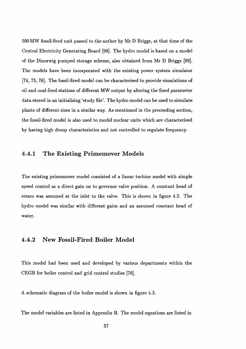
500 MW fossil-fired unit passed to the author by Mr D Briggs, at th a t tim e of the
Central Electricity Generating Board [98]. The hydro model is based on a model
of the Dinorwig pum ped storage scheme, also obtained from Mr D Briggs [99].
The models have been incorporated with the existing power system simulator
[74, 75, 76]. The fossil-fired model can be characterised to provide simulations of
oil and coal-fired stations of different MW output by altering the fixed param eter
da ta stored in an initialising ‘study file’. The hydro model can be used to simulate
plants of different sizes in a similar way. As mentioned in the preceeding section,
the fossil-fired model is also used to model nuclear units which are characterised
by having high droop characteristics and not controlled to regulate frequency.
4.4.1 T he E xisting Prim em over M odels
The existing primemover model consisted of a linear turbine model with simple
speed control as a direct gain on to governor valve position. A constant head of
steam was assumed at the inlet to the valve. This is shown in figure 4.2. The
hydro model was similar with different gains and an assumed constant head of
water.
4.4.2 N ew Fossil-Fired Boiler M odel
This model had been used and developed by various departm ents within the
CEGB for boiler control and grid control studies [78].
A schematic diagram of the boiler model is shown in figure 4.3.
The model variables are listed in Appendix B. The model equations are listed in
57
Appendix C.
Initially, routines simulating the fossil-fired boiler were integrated into the exist
ing power system simulator running on a single MC68000 Tripos system. The
power system simulation with the detailed boiler model incorporated was then
transferred to an IBM PC hosted T800 transputer running the Helios operating
system. At the same tim e as this, other work was being done to integrate the
basic simulator more fully with the Helios parallel transputer environment [76],
and finally, the modifications necessary for detailed primemover simulation were
incorporated into this parallel system.
The basic 500 MW oil-fired model was modified to obtain models of 500 MW
coal-fired units and 660 MW oil- and coal-fired units as outlined in appendix J.
4.4.3 N ew Hydro M odel
This model was developed within the CEGB to study the governor requirements
of the, at th a t time, soon to be commissioned pum ped storage scheme at Dinorwig
[99].
A schematic diagram of the hydro model is shown in figure 4.4.
The model variables are listed in Appendix D. The model equations are listed in
Appendix E.
The detailed hydro model was incorporated into the power system simulator
which ran under the Helios operating system on parallel transputers.
58
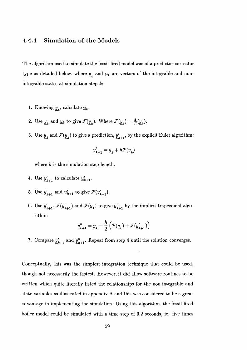
4.4.4 Sim ulation o f th e M odels
The algorithm used to simulate the fossil-fired model was of a predictor-corrector
type as detailed below, where yk and uk are vectors of the integrable and non-
integrable states at simulation step k:
1. Knowing calculate uk.
2. Use and u* to give Where
3. Use yk and F(y_^) to give a prediction, yj.+1, by the explicit Euler algorithm:
sd+: =yJc + h h )
where h is the simulation step length.
4. Use y^+1 to calculate uk+1.
5. Use y^+1 and u'k+1 to give
6 . Use y ' , Jr{yl ) and T iyS ) to give y ” by the implicit trapezoidal algo-AC^“ J . K y i ——Af — f c x l
rithm:
C 1 = h + \ 0 * % )+ ^(sd+i))
7. Compare y^+ 1 and y^+1- Repeat from step 4 until the solution converges.
Conceptually, this was the simplest integration technique tha t could be used,
though not necessarily the fastest. However, it did allow software routines to be
w ritten which quite literally listed the relationships for the non-integrable and
state variables as illustrated in appendix A and this was considered to be a great
advantage in implementing the simulation. Using this algorithm, the fossil-fired
boiler model could be simulated with a tim e step of 0 . 2 seconds, ie. five times
59
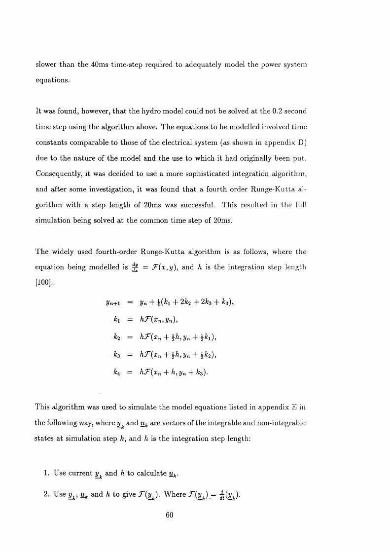
slower than the 40ms tim e-step required to adequately model the power system
equations.
It was found, however, th a t the hydro model could not be solved at the 0.2 second
tim e step using the algorithm above. The equations to be modelled involved tim e
constants comparable to those of the electrical system (as shown in appendix D)
due to the nature of the model and the use to which it had originally been put.
Consequently, it was decided to use a more sophisticated integration algorithm,
and after some investigation, it was found tha t a fourth order Runge-K utta al
gorithm with a step length of 20ms was successful. This resulted in the full
simulation being solved at the common tim e step of 2 0 ms.
The widely used fourth-order Runge-K utta algorithm is as follows, where the
equation being modelled is ^ and h is the integration step length
[100].
Un+1 = Un + l { h + 2k2 + 2k3 -f £4 ),
k\ — h,J~(xnj 2/71)5
k2 = h F ( x n + \ h , y n + ifci),
k3 = h T ( x n + \ h , y n + \ k 2),
&4 — h,^F"[xn h, yn -f- k3^.
This algorithm was used to simulate the model equations listed in appendix E in
the following way, where y k and uk are vectors of the integrable and non-integrable
states at simulation step k , and h is the integration step length:
1. Use current y k and h to calculate uk.
2 . Use i k, uk and h to give T{\t/J . W here F ( y k) = j t {y_k).
60
3. Calculate k\ as above.
4. In a similar manner, use and | to calculate another uk and yk).
5. Calculate k2 as above.
6 . Similarly calculate £ 3 and k±.
7. Use k \ -k 4 to calculate new states, X .+1, as above.
8 . Recalculate uk using whole step length, h, to hold up-to-date values for
non-integrable variables to be displayed and logged.
4.4.5 Load M odels
Changes in system voltage and frequency away from the nominal alters the ef
fective load of the system. This effect was modelled in an algebraic m anner by
introducing ‘load groups’ at each busbar which altered the current injection at
the busbars according to variations in voltage and frequency seen at tha t busbar
[101, 102]. Consequently, the real and imaginary powers were changed from their
nominal or ‘reference’ values using the following algebraic equations:
P = Pref(Pvk + pvivm + PvyV*)(Pfo + Ph ? ^ - ) (4.1)Us
Q = Qrt,(Q*k + + QvyV*)(Qh + Q h (4.2)Us
where Vm is the m agnitude of the busbar voltage,
uj is the derivative of busbar voltage angle, and
Px , Qx are weighting factors, Pvx = 1 etc.
Speed (a;) is calculated as x angle to filter discontinuities, where s is the
Laplace operator.
61
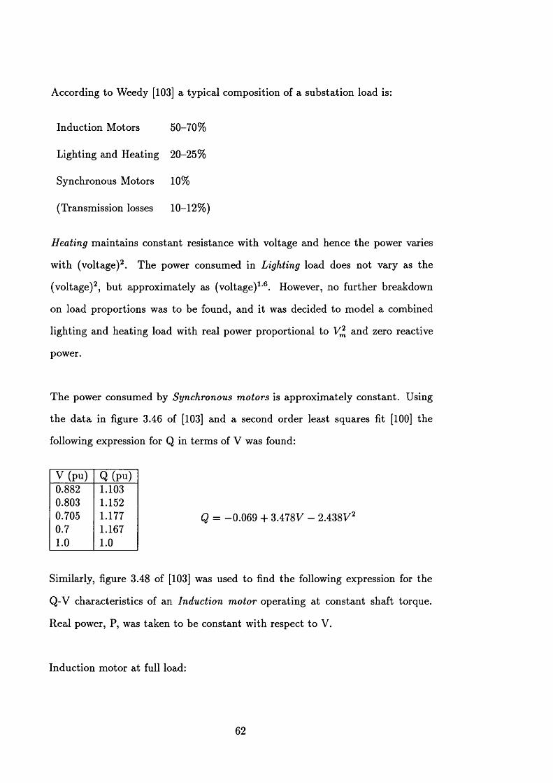
According to Weedy [103] a typical composition of a substation load is:
Induction Motors 50-70%
Lighting and Heating 20-25%
Synchronous Motors 1 0 %
(Transmission losses 1 0 - 1 2 %)
Heating m aintains constant resistance with voltage and hence the power varies
with (voltage)2. The power consumed in Lighting load does not vary as the
(voltage)2, but approximately as (voltage)1,6. However, no further breakdown
on load proportions was to be found, and it was decided to model a combined
lighting and heating load with real power proportional to and zero reactive
power.
The power consumed by Synchronous motors is approximately constant. Using
the data in figure 3.46 of [103] and a second order least squares fit [100] the
following expression for Q in term s of V was found:
Q = -0 .069 + 3.478V - 2.438V2
Similarly, figure 3.48 of [103] was used to find the following expression for the
Q-V characteristics of an Induction motor operating at constant shaft torque.
Real power, P, was taken to be constant with respect to V.
Induction motor a t full load:
V (pu) Q (pu)0.8820.8030.7050.71 .0
1.1031.1521.1771.1671 .0
62
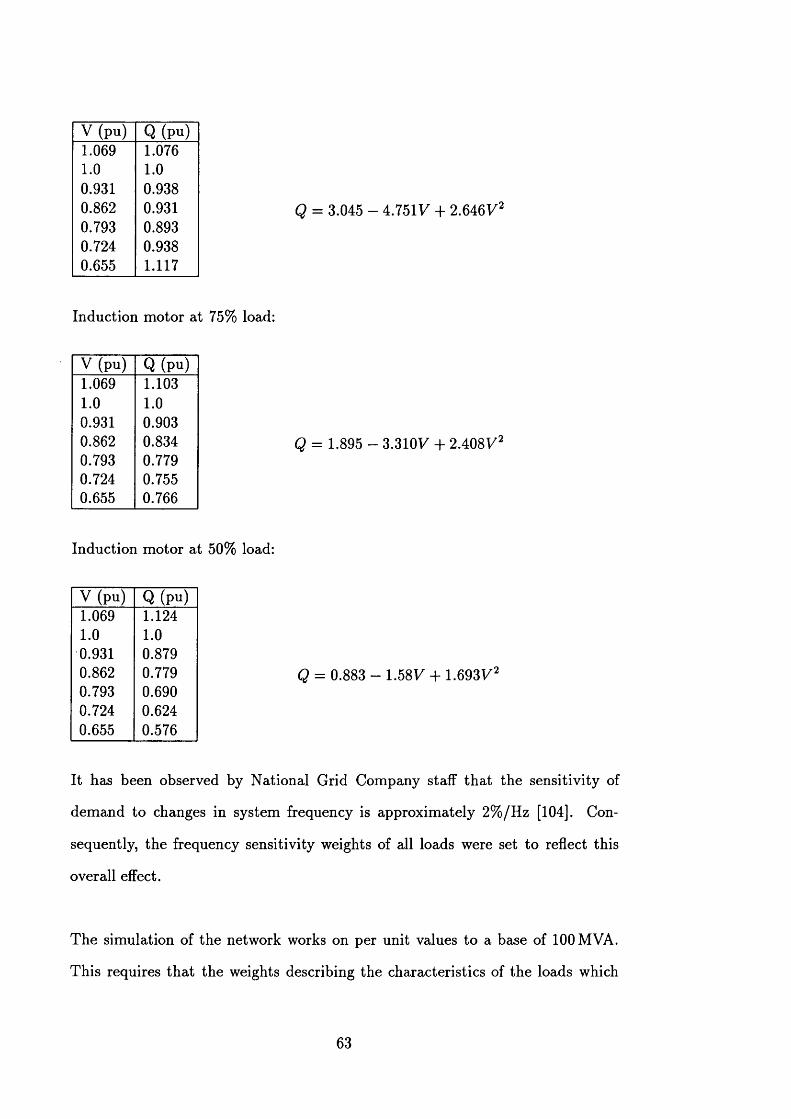
V (pu) Q (pu)1.069 1.0761 .0 1 .0
0.931 0.9380.862 0.9310.793 0.8930.724 0.9380.655 1.117
Q = 3.045 - 4.751V + 2.646V2
Induction motor at 75% load:
V (pu) Q (pu)1.069 1.1031 .0 1 .0
0.931 0.9030.862 0.8340.793 0.7790.724 0.7550.655 0.766
Q = 1.895 - 3.310V + 2.408V5
Induction motor at 50% load:
V (pu) Q (pu)1.069 1.1241 .0 1 .0
0.931 0.8790.862 0.7790.793 0.6900.724 0.6240.655 0.576
Q = 0.883 - 1.58V + 1.693V2
It has been observed by National Grid Company staff th a t the sensitivity of
demand to changes in system frequency is approximately 2%/Hz [104]. Con
sequently, the frequency sensitivity weights of all loads were set to reflect this
overall effect.
The simulation of the network works on per unit values to a base of 100 MVA.
This requires th a t the weights describing the characteristics of the loads which
63
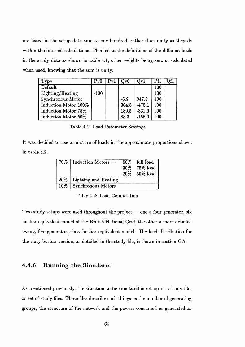
are listed in the setup data sum to one hundred, rather than unity as they do
within the internal calculations. This led to the definitions of the different loads
in the study data as shown in table 4.1, other weights being zero or calculated
when used, knowing th a t the sum is unity.
Type PvO P v l QvO Q vl P fl QflDefaultLighting/Heating Synchronous Motor Induction Motor 100% Induction Motor 75% Induction Motor 50%
- 1 0 0
-6.9304.5189.5 88.3
347.8-475.1-331.0-158.0
1 0 0
1 0 0
1 0 0
1 0 0
1 0 0
1 0 0
Table 4.1: Load Param eter Settings
It was decided to use a m ixture of loads in the approximate proportions shown
in table 4.2.
70% Induction Motors — 50% full load30% 75% load 20% 50% load
2 0 % Lighting and Heating1 0 % Synchronous Motors
Table 4.2: Load Composition
Two study setups were used throughout the project — one a four generator, six
busbar equivalent model of the British National Grid, the other a more detailed
twenty-five generator, sixty busbar equivalent model. The load distribution for
the sixty busbar version, as detailed in the study file, is shown in section G.7.
4.4.6 R unning th e Sim ulator
As mentioned previously, the situation to be simulated is set up in a study file,
or set of study files. These files describe such things as the number of generating
groups, the structure of the network and the powers consumed or generated at
64
the different busbars. Param eter settings for individual model units such as
generating sets, and primemover types are also given. For the investigations
reported here, two studies were used. The full supergrid system to be modelled
is shown in figure 4.5(a). The first study modelled this system as an equivalent
four generators, with a network of six busbars as shown in figure 4.5(b). The
CEGB group models the equivalent of 21 identical generators, DINORWIG six,
NWALES one and SCOTLAND five. Appendix F lists the study files describing
this equivalent system. The second study modelled the grid as an equivalent
twenty-five generators and sixty-six busbars. This study is based upon that used
by Berry [75], with modifications to allow frequency and voltage sensitive loads
as described in section 4.4.5 and to model the Dinorwig pum ped storage scheme
in North Wales as six independant generating groups rather than one common
group. The network diagram of this system is shown in figure 4.5(c). Appendix G
lists the study files describing this system.
On first running the simulator, the m aster study file is read and the data copied
to the sim ulator’s internal database, with conversions to per unit values as ap
propriate. Using the network interconnection data and the data for generated
and consumed powers, a to tal network adm ittance m atrix is constructed. The
simulation then proceeds to solve the generator and load equations in parallel
to produce current injections at the network nodes. This stage is followed by
the calculation of the network equations to solve for the network voltages. The
network calculation may also be performed in parallel if appropriate hardware is
available (see section 5.2.1 for the different hardware setups available to run the
simulator) and the network is complex enough to justify a parallel solution [76].
A check for convergence of the network solution is made, and these two stages
re-iterated until the solution converges. The simulator then progresses on to the
next model time step.
65

Under steady state model conditions, each step requires only one iteration. How
ever, when the model states are changing rapidly, several iterations may be re
quired. Real-time operation can be achieved if the tim e taken for each model
tim e step is the same as the true ‘clock’ tim e tha t th a t step represents, ie. 2 0 ms
in the particular studies reported here. W hen model states change and more than
one iteration per step is required, the simulation may slow down. As long as the
solution for one iteration takes less than the tim e alloted, once the model states
settle down, the simulator can run fast for a while until it has caught up the lost
time. This is known as ‘soft’ real-time operation, as the simulator falls behind
‘clock’ tim e while it is busy, and catches up again during steady state operation,
meaning th a t over an extended period it follows ‘clock’ time.
How quickly a model step can be calculated depends on the complexity of the
problem, ie. the size of the network and the detail of the generator and load
models, and the processing power available. The most powerful computing facility
available to the author was the sixteen transputer rig described in section 5.2.1
and by Chan [76]. The four machine study of appendix F could be run in real
tim e using one Transputer. However, the twenty-five machine study including
frequency and voltage sensitive loads was rather slower than real-time when run
on all the processors available.
For the extent of investigations covered by this report, real-time is not of impor
tance, other than meaning less tim e to wait for results to be acquired. However,
in any future work to test operational controller software prior to installation on
a live system, a real-time simulation would be invaluable.
66
4 .4 .7 C on tro llers
4.4.7.1 Boiler Control
It was necessary to add a closed loop boiler control system to the fossil-fired
primemover model. W ithin a power station boiler a number of variables need to
be controlled, such as steam tem perature and the pressure within the furnace.
However, as far as the characteristics presented to the grid are concerned, it is
the load control system which is the most im portant. Hence, the simplifying
assumption was made th a t all other controls held their outputs constant and
were not modelled in detail.
The control of load output of a power station unit is part of a two-input, two-
output system. The inputs are the fuel flow into the furnace and the positions
of the governing valves (modelled as one main governor valve in this simulation).
The outputs are the load of the unit, the MW, and the steam pressure a t the
output of the secondary superheater.
There are a number of controller structures which can be used with this multi-
variable system. The most traditional system, known as boiler-follows-turbine
(B FT), uses the position of the governor valve to control load, L, and the fuel in
put to control the changes in pressure, Ps, inflicted by the movement of the valve.
This is shown in figure 4.6. A second structure is known as turbine-follows-boiler
(TFB) and is shown in figure 4.7. In this case, the governor valve is used to
control the steam pressure, and changes in load are affected by altering the fuel
input to the boiler. This method has an advantage in terms of wear and tear
on the boiler as it does not allow such severe transients in pressure as the BFT
67
method. However, it requires modifications in order to be responsive enough to
load changes required for the regulation of grid frequency. The two figures also
illustrate the means by which the unit control is modified in order to help regulate
the system frequency, / .
The initial control system implemented in the simulation was of a multi-variable
type based on one installed at a British power station [105]. This was chosen
for ease of access to the algorithms. Later, a BFT system based upon the model
param eters was designed as described in section 4.4.7.2. This was to enable the
characterisation of controllers for different size of units, since the multi-variable
controller was designed specifically for tha t station and was found not to be so
successful on models of other sized units.
4.4.7.2 D esign o f a Boiler-Follows-Turbine U nit Control System
A block diagram of the fossil-fired boiler model is shown in figure 4.8. The vari
ables and param eters relate to the definitions given in appendix B. Two control
loops need to be designed for the unit control system — a loop controlling su
perheater outlet pressure by varying the fuel input, and a loop controlling load
output by varying the governor valve position. Because of the wide difference in
the tim e constants dominating the plant of these two loops, they can be designed
quite separately. Since the plant is non-linear, a linearised reduction of each loop
was made at several different operating points. In general, the variation in pres
sure to allow operation at different unit power outputs is quite small compared
to the range of the load output, ie. the relative operational variation in MW is
rather larger than the corresponding variation in pressure. Consequently, it was
decided to form a reduced model of each loop at varying loads, ie. MW, but
68
constant superheater outlet pressure.
Appendix H details the derivation of the linearised models used in the design of
the pressure control loop, whilst appendix I details the corresponding derivation
for the load loop. The figures used in these illustrations are for the 500 MW
oil-fired boiler model.
P re s s u re L oo p Neglecting d.c. gain, the following fourth order equivalent
transfer functions were derived for the plant in the pressure loop at different load
levels.
G{s )\170Mw g4 + o 5 7 9 0 6 s 3 + o.0966963s2 + 0.00418037s + 7.4823.10-7
(4.3)
G(s )\250m w = s4 + 0 4 9 8 6 3 3 s 3 + 0.0757525s2 + 0.00324256s + 7.4828.10-6
(4.4)
1G (s)| 390 M W =
G (s)| 490 M W =
s 4 + 0.43117s3 + 0.0579801s2 + 0.00240117s + 1.03934.10-5
(4.5)
1
s4 + 0.408192s3 + 0.0521148s2 + 0.00216454s + 1.38646.10~5
(4.6)
A proportional plus integral, PI, controller was chosen to control this system and
appropriate gains acquired through the design process outlined in appendix H.
Subsequently, it was found th a t the following gains adequately controlled the su
perheater outlet pressure of the non-linear 500 MW oil-fired boiler model through
out the load range:
69
K p = 0.6366 (4.7)
Ki = 0.006366 (4.8)
where K p and Ki are the controller’s proportional and integral gains respectively.
This leads to a controller of the form shown in figure 4.9.
L o ad L oop Using a similar block diagram reduction technique the following
transfer functions were obtained for the plant in the load loop, as outlined in
appendix I.
47322.3(s2 + 4.42745s + 0.522409) (s)|i70m w - ^ 3 + 5 8 9 9 2 7 s 2 + 6.81264s + 0.0230386
19371.l ( s 2 + 3.29252s + 0.370477) l4 , n,(s)|250MW' “ s 3 + 4.76775s2 + 5.07439s + 0.151419 ' ' '
20294.1 (s2 + 2.30094s + 0.243892)(s ) |3 9 o w - ^ + 3 7 g 0 7 7 s 2 + 3 .5 5 5 9 5 ^ + q.388158 * ' ’
_ 19101.4(s2 + 1.94571s + 0.197154)(s ) |4s o w ^ + 3 .4 2 7 9 8 s2 + 3.012003s + 0.678126 ' *
To achieve zero steady state step error and reasonable speed, integral, I, control
is all th a t is required to control a system of this form as shown in figure 4.10.
Subsequently, it was found th a t the following gain adequately controlled the load
70
output of the non-linear 500 MW oil-fired boiler model throughout the load range,
as detailed in appendix I.
I<i = 0.00025 (4.13)
Controller Im plem entation The model of the boiler assumed the unit was
controlled by a digital rather than analogue controller, as is the case in m od
ern power station practice. Therefore, to implement the controllers within the
simulator software they needed to be digitised. This digitisation is shown in
appendix K for both PI and I controllers.
A similar design to th a t explained above, and outlined in appendices H and I
was performed for a 500 MW coal-fired boiler, leading to the use of the controller
gains listed in table 4.3 and as specified in the simulation study files.
Boiler Type Pressure Loop Load LoopI<P I<i K p
Coal 500 MW 0.6295 0.003777 0.00025Oil 500 MW 0.6566 0.006566 0.00025
Table 4.3: Boiler-Follows-Turbine Controller Gains
By simulation, it was found th a t these gains were also adequate to control the
660 MW boiler models, whose dynamics were not very much different to the
500 MW units.
4.5 Sum m ary
This chapter has presented details of the simulation used for the study of auto
m atic load-frequency control on the British grid system. The need for simulations
in such work has been discussed together with examples of other simulations.
71

The development of power system simulation at the University of Bath has been
described and further developments necessary for the current study have been
presented. Detailed models have been given for different primemover types and
for loads sensitive to frequency and voltage variations. Finally, load control of
the generating units has been described.
72
C hapter 5
C om puting Facilities
A variety of computing facilities was used during the course of this work for both
the off-line development and analysis, as well as the on-line simulation studies.
This chapter describes some of the hardware and software used.
5.1 Off-Line F acilities
A good deal of the off-line work, including linearisation of the fossil unit mod
els and the corresponding design of unit controllers, was performed on a Mo
torola MC68000 based multi-user, multi-processor machine under the Tripos op
erating system [87, 88, 89]. This hardware was based on the single board computer
units described by Dale [74]. The original Tripos was a single-user, multi-tasking
operating system for small computers initially developed at the University of
Cambridge and modified at the University of Bath to also support a multi-user,
multi-processor environment. Tripos itself is w ritten in the BCPL high level lan
guage and also supports FORTRAN, LISP, PASCAL and ANSI C. A number of
facilities were available on this system, such as the symbolic m athem atics pro
gram REDUCE [106], a root locus generating program and a graph plotter. The
73
first C version of the B ath University Power System Simulator was also avail
able on this system having been translated from the original BCPL version [92].
Consequently, this was a convenient environment for the initial development of
generating unit models and off-line analyses. However, this system did not offer
sufficient computing power to run the full power system simulator at a reasonable
speed.
5.2 O n-L ine F acilities
5.2.1 Hardware
In order to use the standard power system simulator to simulate yet more com
plex systems in real-time, more powerful computing facilities were needed. At
this time, the simulator programs were w ritten in BCPL and ran on a Mo
torola MC68020 based parallel com puter under the Tripos operating system as
described by Berry [75]. Decisions were taken with regard to the best way forward
to improve the performance of the power system simulator. O ther simulation
work on diesel engines within the departm ent also required the use of more pro
cessing power and this led to the development of a new parallel computer based
on the Inmos Transputer [107]. The other options available at the tim e were to
redesign the existing MC68020 based computer using new high speed components
or to use an upgraded version of the same family of processors, for example, the
MC68030, or to use the then new Intel 80386 processor in a new com puter de
sign. However, it was found th a t the transputer based option promised the best
improvement in performance still at a reasonable cost.
The standard means of inter-processor communication in a transputer system
74
is via transputer links. However, this did not provide sufficient communication
bandw idth for the diesel engine simulation which had a high communication bur
den in relation to the calculation burden on the processors. Hence, a shared
memory architecture was designed together with a new fast multiprocessor back
plane bus [108] as well as the transputer link bus. Building an in-house parallel
com puter based on the T800 transputer [94] was found to be less costly than
buying a commercial system with all of these facilities.
It was felt th a t the new transputer based parallel com puter would also offer signif
icant improvements in the performance of the power system simulator and allow
more complex systems to be modelled in real time. Initially, it was estim ated
tha t the communication burden of the power system simulation would m atch the
calculation burden when the transputer links were used as the communication
mechanism. Using the shared memory for communication would lead to a saving
approaching 50% of the to tal processor burden by significantly reducing the com
munications burden. However, in practice, it was found th a t the T800 transputer
did not improve the calculation performance as well as the initial da ta suggested
it m ight. Consequently, the calculation burden was still significantly higher than
the communication burden rather than being comparable. In this situation, the
saving to be gained by using shared memory as the communication mechanism
represented only about 15% of to tal processor burden. In order to use the shared
memory instead of the standard transputer links for communication, it was nec
essary to provide special software primitives for accessing the shared memory.
This meant tha t non-standard and non-portable software would have to be used
if advantage was to be taken of the shared memory communication mechanism.
In the case of the power system simulator, it was decided th a t the realisable
15% saving was not sufficient to warrant losing portability of the software and
consequently this facility was not used.
75
A block diagram of the T800 based parallel computer is shown in figure 5.1. The
machine is housed in several 19-inch racks and has sixteen processing nodes per
rack. Each processing node consists of an Inmos T800 transputer, 1 M Byte of
dynamic RAM (DRAM), a multiprocessor bus interface, local and multiprocessor
bus arbiter logic and high speed line drivers to connect the transputer links to
other boards via the backplane. A block diagram of the T800 processing node is
shown in figure 5.3.
A transputer is a single VLSI micro-processor with on-chip memory, a central pro
cessing unit and communication links for direct connections to other transputers.
The T800 transputer used in the parallel computer has a 32 bit bus, 4 KBytes
of on-chip memory, a 64 bit floating point co-processor and four direct memory
access (DMA) controlled serial links [94]. Figure 5.2 shows a block diagram of
the T800 transputer.
The T800 exploits fast on-chip memory by having only a small number of registers
and simple instructions. It uses multiplexed address and data signals in its 32 bit
memory bus. A built-in memory controller provides DRAM control and refresh
timing. The internal processor speed is link selectable and is generated by a 5 MHz
external clock. The transputer can be booted either from a communication link
or from a ROM (Read Only Memory). All the processing nodes in the parallel
com puter are booted via links.
The inpu t/ou tpu t (10) system for the transputer based parallel com puter was
developed by Hafeez and is based on the Philips SCC68070 micro-processor [109].
Figure 5.4 shows a block diagram of the 10 board. The SCC68070 has an on-
chip memory management unit, a two channel DMA controller, a serial interface,
and inter-integrated circuit (I2C) bus interface and a timer. The 10 system built
76

around it exploits these features to connect to external devices such as disk drives,
printer and a console. Floppy disks, a hard disk drive and a tape stream er are
available. In order to connect the 10 board to the other T800 based boards in
the system, a bi-directional, two wire transputer link is provided via an IMSC012
link adapter.
A graphics board is also provided which consists of a T800 transputer, a Philips
SCN66470 Video and System Controller (VSC), a Philips 68070 micro-processor,
keyboard and mouse interfaces, a colour palette and two banks of memory. A
block diagram of the board is shown in figure 5.5. The 4 MBytes of local memory
is available to the operating system and is refreshed by the T800. The other
1 M Byte bank is used for video and display data and is controlled by the VSC.
The hardware just described forms a complete computing system. However, in
these studies, an alternative arrangement was used. It was convenient to use extra
space on the graphics card just described for other circuitry. In this arrangem ent,
differential line driving circuitry was employed to provide an interface between
the sixteen transputer rack and a remote computer. The parallel com puter is
connected to a commercial transputer card [110] plugged into a personal com
puter (PC) [111] in an adjacent room. The physical arrangem ent of the hardware
is such th a t one transputer link on the plug-in card is used for PC -transputer
communications while the remaining three links connect into the parallel com
puter via the differential lines. Further circuitry, also situated on the graphics
board, provides hard-wired links to connect together the sixteen transputers of
the parallel computer, the transputer on the graphics card and the transputer
plugged into the PC to form a network as shown in figure 5.6. Peripheral devices
such as monitor, graphics monitor, keyboard and disks are available via the PC.
Hosting the transputer network via a PC in this way was not only a convenient
77

interface to the parallel computer but also provided flexibility and allowed the use
of readily available PC software for off-line work. For the smaller simulations it
was adequate to use just the single transputer plugged into the PC which allowed
other users to take advantage of the computing power of the multi-processor com
puter. W hen it was required to use the parallel computer, it was necessary to
connect the differential line between the transputer rack and the PC and to run
the appropriate operating system for the network.
5.2.2 Software
The operating system chosen to run on this hardware was Helios [93]. Helios is
a multi-user, multi-processor distributed operating system designed to run on a
wide range of multi-processor architectures and originally targetted at transputer
based networks. Much of Helios is w ritten in C and C was chosen as the high level
language in which to implement the newest version of the power system simulator.
Helios is intended to provide a Unix compatible programming interface.
The natural choice of operating system for a transputer based com puter might
have seemed to be the Transputer Development System (TDS) supported by
the manufacturers, Inmos. This would have encouraged the use of OCCAM as
the high level progamming language, the transputer having been developed to
exploit the OCCAM model of parallel programming. However, OCCAM had a
number of disadvantages. It did not support dynamic memory allocation making
it unsuitable for use in complex programs. It was a specialist language with
little prospect of being ported to a large number of other processors. This meant
th a t if future versions of the simulator were to be run on other processors, the
software would have to be rew ritten in yet another new language. Finally, this
78
option would not have allowed useful programs and tools to be readily ported
from other systems such as Unix based machines.
The Helios/C solution did not suffer from these disadvantages. C was a language
which was becoming increasingly popular and supported on a wide range of pro
cessors. This would m ean little or no re-writing of code to port the sim ulator to
other hardware. It wrould also mean th a t other applications w ritten in C could
easily be ported to the Helios environment. Helios provides a Unix like user in
terface which would make the simulator more readily accessible to users already
familiar w ith Unix or similar environments. It was also hoped th a t Helios would
be developed to run on other new processors as technology progressed. However,
in the event, the use of C has proved to be the most useful factor in allowing
serial versions of the simulator to be run on a variety of different computers w ith
out the Helios operating system, including SUN and APOLLO workstations and
IBM PCs [76]. To take full advantage of the processing power available from
the transputer based parallel com puter to run the more complex simulations in
real-time, Chan took advantage of Helios’ explicit message passing protocols and
produced a parallel version of the simulator based on the typical Helios client-
server model [76]. It was to this version of the simulator th a t the more detailed
models of this study were added.
5.2.2.1 H elios
Helios controls all the resources available within a transputer network, and pro
vides a consistent mechanism for accessing these resources, hiding the distributed
nature of the architecture from the user. A standard server program for the host
machine acts as an interface to the transputer network and allows the user to
79

access all the standard features of the host environment. The main components
of Helios are the nucleus, servers, the posix library and the user interface.
The user interface is provided by a task called Shell tha t acts as a command line
interface to the operating system and enables the user to create and control jobs
interactively, both in the background and the foreground. Shell includes various
shorthand techniques to save typing and personalisation methods to enable users
to define their own commands. Several shells may be run simultaneously.
The nucleus is the minimum system th a t must be present on every processor in
the network. Its prime purpose is to control the resources of a single processor
and to integrate it into the global system. The nucleus consists of six parts:
Kernel, System Library, Server Library, Utility Library, Processor Manager and
Loader. The Kernel is responsible for the processor hardware and provides low-
level calls such as message passing, semaphore synchronisation, and creating and
destroying processes. The System Library provides the basic interface between
clients and servers containing library routines such as Open() and R ead(). The
Server Library exists to assist in writing Helios servers and the Utility Library
provides a num ber of further library routines. The Loader is a Helios server
which takes care of pieces of code loaded into its processor, and which ensures
th a t code is shared between programs where possible. The Processor Manager
is also a server which allows clients to run programs or tasks on th a t processor.
It takes care of signals sent to a particular task and ensures tha t any resources
used by a program are freed when a program exits.
Helios is based on the client-server model of computing in which a client program
wanting some service sends a message to a server program which performs the
operation and returns a reply message. For example, to read data from a file it is
80
necessary to interact with a file server. A general server protocol (GSP) defining
the structure of these messages is supported by all Helios servers. Each server
consists of a single task within whic'h a single dispatcher process is dedicated to
receiving the requests and queuing them for attention by a second process. This
second process may be either a static process, a dynamically created process or
a pool of worker processes to handle each request as it arrives.
The posix library is provided in Helios to make it compatible- with Unix. This
facility aids portability of existing programs and tools from the Unix environment
to Helios.
5.3 Sum m ary
This chapter has described the hardware facilities and programming environments
available for the development of the power system simulator as well as for off
line analyses. The on-line simulation work was performed on a Transputer based
parallel computer hosted by a PC and running the Helios operating system. The
simulation software was w ritten in C. Several environments were available for off
line work including the Helios machine, the PC running the MSDOS operating
system and another in-house multi-tfser com puter based on M otorola MC68000
processors running the Tripos operating system and using a variety of program
ming languages.
81
C hapter 6
Four M achine Studies
6.1 V alid ation o f F ossil M od el
6.1.1 Stored Energy Tests
The fossil unit model was validated by comparing its response to stored energy
tests with those of the model on which it was based which had itself been validated
against stored energy tests performed at Ratcliffe Power Station in October 1969
[98]. The tests were performed by forcing a step change in governor valve position
from a part load condition to fully open. The resulting transients in load and
pressure characterise the plant. Results of the tests performed on the model are
shown in figures 6.1, 6.2 and 6.3. These compare with the base results as shown
in table 6.1.
The current model results can be seen to compare quite well with those of the
earlier model. The discrepancies with the plant test results are mostly due to
effects which have not been modelled such as the fact th a t superheater spray
flow is not actually constant as is modelled and th a t steam tem perature is also
82
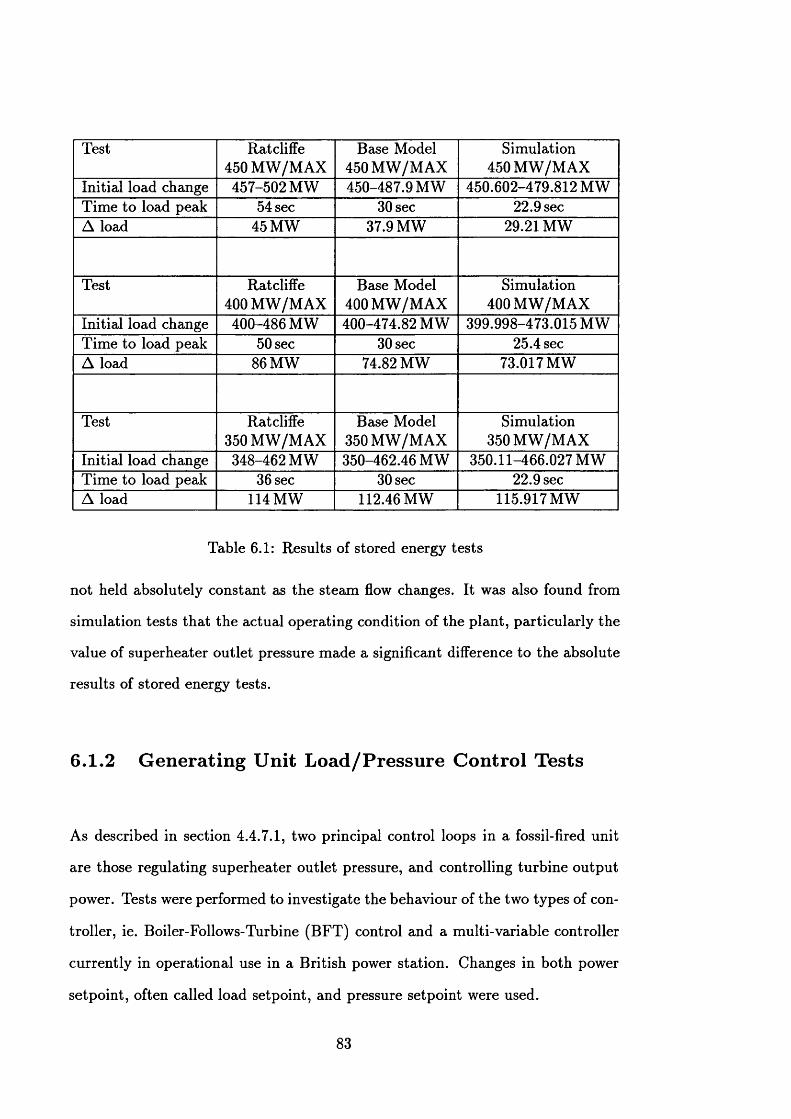
Test Ratcliffe 450 M W /M AX
Base Model 450 M W /M AX
Simulation 450 M W /M AX
Initial load change 457-502 MW 450-487.9 MW 450.602-479.812 MWTime to load peak 54 sec 30 sec 22.9 secA load 45 MW 37.9 MW 29.21 MW
Test Ratcliffe 400 M W /M AX
Base Model 400 M W /M AX
Simulation 400 M W /M AX
Initial load change 400-486 MW 400-474.82 MW 399.998-473.015 MWTime to load peak 50 sec 30 sec 25.4 secA load 86 MW 74.82 MW 73.017 MW
Test Ratcliffe 350 M W /M AX
Base Model 350 M W /M AX
Simulation 350 M W /M AX
Initial load change 348-462 MW 350-462.46 MW 350.11-466.027 MWTime to load peak 36 sec 30 sec 22.9 secA load 114 MW 112.46 MW 115.917MW
Table 6.1: Results of stored energy tests
not held absolutely constant as the steam flow changes. It was also found from
simulation tests th a t the actual operating condition of the plant, particularly the
value of superheater outlet pressure made a significant difference to the absolute
results of stored energy tests.
6.1.2 G enerating U nit L oad/Pressure C ontrol Tests
As described in section 4.4.7.1, two principal control loops in a fossil-fired unit
are those regulating superheater outlet pressure, and controlling turbine output
power. Tests were performed to investigate the behaviour of the two types of con
troller, ie. Boiler-Follows-Turbine (BFT) control and a multi-variable controller
currently in operational use in a British power station. Changes in both power
setpoint, often called load setpoint, and pressure setpoint were used.
83
6.1.2.1 Load Setpoint Changes
Figures 6.4 and 6.5 show the results of a load setpoint increase in the one
NWALES unit (figure 6.4 for the BFT, and figure 6.5 for the multi-variable con
trollers). In order to m aintain the overall load/generation balance, this has been
accompanied by a decrease in load setpoint in the twenty-one CEGB units. In or
der to reduce the effect of load changes on the pressure control, the setpoint, Lap,
is ra te limited and ramps towards the new desired value, L&v. From the NWALES
generation traces it can be seen th a t both controllers enable the generation, Pmw,
to closely follow the ramping setpoint, L sp. The multi-variable control is a lit
tle tighter but also has slightly more overshoot. Because the twenty-one CEGB
units can complete their small load change faster than the single NWALES unit
can complete its rather larger change (since each individual unit has the same
rate limit on Lap), during the load change there is a load/generation imbalance
which results in an error in frequency. For this test, there is no frequency error
term in the L aps so th a t they simply follow Ldv• However, the speed control onto
the governor valves forces an offset proportional to frequency error in the valve
position Zgv away from its nominal position set by the speeder motor, Zgvc. This
effect prevents the CEGB units from following the L ap ram p but rather to lag it
to reduce the frequency error. This mismatch of Zgv and Zgvc can clearly be seen
in both CEGB governor graphs (figures 6.4(b) and 6.5(b)). The most obvious
differences in the behaviour of the two types of unit controller may be seen in
the pressure and fuel flow graphs. In the B FT case, two separate control loops
operate, one altering speeder m otor position in order to control load and the
other varying fuel flow to regulate pressure. In figure 6.4(b), the pressure varia
tions, P 2 ? caused by the changes in governor valve position can be seen together
with the changes in fuel flow, M /u, required to correct them . The multi-variable
controller does not trea t the system as two independent loops, but rather calcu
84
lates changes in both Zgvc and M fu required to control both P2 and Pmw. This
controller achieves a tighter pressure control than the BFT controller, as shown
in figure 6.5(b), by varying the fuel flow more rapidly. This comes about because
the B FT controller requires the pressure to have changed before it has an error
to correct which it reacts to fairly slowly, whereas the multi-variable controller
is able to, in effect, anticipate the changes required in fuel flow immediately to
support the change in load.
6.1.2.2 Pressure Setpoint Changes
Figures 6.6 and 6.7 show the results of a pressure setpoint decrease in the single
NWALES unit. In this case, the load controllers are operating in a sustained
mode whereby L sp contains a component proportional to frequency error as can
be seen in all the generation graphs where L sp is slightly offset from L&v because
of the small error in frequency.
As in the case of the load setpoint change, the pressure setpoint, Psp, is rate
limited and ramps towards the desired value, rather than following it directly.
However, it may be seen from the NWALES pressure graphs th a t the dynamics
of this particular unit are rather too slow to follow this ram p very closely.
Considering the BFT case (figure 6.6(b)), it can clearly be seen how the fuel flow,
M /u, reduces at the start of the downward ram p of the setpoint. Gradually, the
pressure, P2 , starts to decrease. The decrease in pressure has an effect on the load
loop since it leads to a decrease in steam flow. Thus, in order to m aintain the
power output, the load loop increases the governor valve position to compensate
for the decrease in pressure. The load loop has rather faster dynamics than the
85
pressure loop and easily copes with the speed of the pressure change. This results
in only a small fluctuation in the power, Pmw> away from its setpoint, Tsp, as the
pressure changes (see figure 6.6(a)). Because the NWALES generation fluctuates
only very slightly, there is no noticeable effect on the other generators.
In the case of the multi-variable controller, figure 6.7(b) illustrates how both
inputs, Zgvc and M fu, are varied rather more rapidly to effect the change in
pressure. However, it would appear from the P2 trace th a t this controller is not
really appropriate to the very slow dynamics of this loop, and, in particular,
M fu appears to be changed too quickly. There is interaction apparent in Pmw
which is sufficient to effect slightly the other generators. The structure and
gains for this controller were taken from an operational load controller which
had been specifically designed for tha t particular plant using a discrete “black -
box modelling” approach. Consequently, it was not possible to “tune” this loop
simply since the physical meaning of the gains in this type of controller are not
evident as they are in the PI type of controllers used in the BFT design. Hence,
the BFT design was used throughout the following results since it was more
flexible.
6.2 V alid ation o f H ydro M od el
The hydro model used for these studies was based upon the model of Dinorwig
power station described in [99]. The current simulation of Dinorwig was validated
with reference to this original model.
86
6.2.1 Lookup Tables for Non-Linear Characteristics
Certain model non-linearities such as the torque/speed and discharge/speed char
acteristics were implemented within the simulation by means of a lookup table.
To validate the operation of this code, it was used to reproduce graphs of these
characteristics which were then compared to the original characteristics given
in [99], figures 2.2 and 2.3. The reproduced graphs are shown in figure 6.8 and
compare well with those of [99].
6.2.2 R esponse to M anual Ram ping o f G uide Vane P osition
A similar validation test to tha t used in [99] was performed whereby the guide
vanes were ram ped open at their maximum rate. The results of this test are
shown in figure 6.9. The initial conditions were such tha t the DINORWIG group
representing all six units was spinning in water, synchronised to the grid, but
delivering no power. The results compare quite closely with those given in fig
ures 3.1 and 3.2 of [99]. The small discrepancies in absolute level of some variables
are due to the difficulties of matching the operating conditions exactly. However,
the dynamic responses m atch closely.
6.2.3 R esponse to Power Setpoint Change
In [99] the model was used to perform a series of tests to investigate the gover
nor characteristics of Dinorwig, some of which were responses to power setpoint
changes. One of these was repeated with the current simulation to further val
idate the m atching of the two models. These results are shown in figure 6.10.
87
The conditions of this test were similar to those in figure 6.18 of [99], where the
input was a 0.2 pu. power setpoint change. There is fairly good matching of the
dynamics as seen before. However, there is some discrepancy in the levels of some
variables. This is due to the different operating points at which the simulations
were performed and differences in the simulations outside of the dynamics of just
the hydro system, ie. in the modelling of the rest of the power system to which
the hydro model was connected.
6.3 S y stem Split S tu d ies
It has been proposed (see section 3.5.3) to operate the system as two separate
control areas such tha t the frequency in each area may be controlled together
with the power flow on the tie-lines linking the two areas. The system charac
teristics required for the design of the controller can be determined from system
split tests [20]. The following discusses a series of results of system split tests
on the four machine simulation which were used to determine the system power-
frequency characteristics of the two areas. In these tests, all tie-lines between
the two areas were opened whilst the power being carried by them was approxi
m ately 565 MW. The accompanying figures illustrate the resulting frequency and
generation changes.
88
6.3.1 System w ith D inorwig G enerating and Insensitive Loads
6.3.1.1 Sustained U nit Controllers w ith 5% M C R /m in Setpoint R ate
Lim its
Figure 6.11(a) shows the response of the frequencies in the two areas follow
ing the disconnection of the inter-ties and the resultant changes in generation,
while figure 6.11(b) shows the corresponding mechanical torque changes and the
movements of the speeder motor position (Zgvc) and the governor valve (Zgv).
SCOTLAND Generation in figure 6.11(a) illustrates clearly in Pmw the immediate
decrease in electrical load on the Scottish machines when the tie-lines are opened.
There are five machines each with a decrease in load of about 113 MW, ie. a
to tal of 565 MW, corresponding to the power being exported by the tie-lines
prior to the split. This decrease in electrical load causes an imbalance between
the electrical load and the mechanical power into the generator (as illustrated
by SCOTLAND Mechanical Torque, Tm, in figure 6.11(b)). This causes the
machine to increase in speed (as illustrated by f sco in figure 6.11(a)). The increase
in speed causes the governor speed controller to close the governor valve (Zgv
in SCOTLAND Governor, figure 6.11(b)) which, in turn , causes a reduction in
mechanical torque produced (SCOTLAND Tm). During this time, the unit load
controller is attem pting to m atch generation, Pmw,, with the setpoint, L sp. In
response to the rise in frequency, L sp is reduced by the controller to help correct
th a t rise. However, the rate limit on L sp prevents it from falling very quickly
and there is a substantial error between L ap and Pmw. This error causes the load
controller to increase the speeder motor position Zgvc. This does not, however,
cause an increase in the governor valve position since the speed controller is
89
forcing an offset between Zgvc and Zgv proportional to the frequency error. Once
Zgvc reaches its upper lim it, Zgv is able to remain at a level which matches
the mechanical torque, Tm, with the electrical load, Pmw, so th a t the frequency
remains constant. A much longer run reveals tha t once L sp has reduced to the
level of Pmiv, the governor m otor comes off its limit and allows the offset between
Zgvc and Zgv to reduce Tm so th a t the frequency falls back towards 50 Hz. This
long term trend is further discussed in section 6.3.3.
The response of the machines in England and Wales is a little different because
of the regulating action of DINORWIG. W hen the system splits, the electrical
load on the machines immediately increases. DINORWIG is in a mode whereby
it is responding only to errors in frequency and is not also trying to m aintain its
generation at any particular setpoint. This means th a t after the initial increase
in generation, DINORWIG continues to rise taking increasingly more of the share
of the ex tra load. This allows the CEGB and NWALES machines to reduce their
generation back towards their setpoints. Because of the rate limit on the CEGB
and NWALES setpoints, L sp, the response is rather slow and oscillatory until all
the England and Wales machines settle out with a proportionate share of the
extra load.
The situation of a slow oscillatory response due to rate limits reflects what can
happen in practice. However, it is difficult to determine what is the frequency
change due to the sudden load/generation imbalance. It would be impractical
to wait for the system to reach a steady state condition as other disturbances
would be likely to occur before th a t happened. Consequently, the simulation was
repeated with no rate lim it on the L sps of the fossil units.
90
6.3.1.2 Sustained U nit Controllers w ithout Setpoint R ate Limits
Figure 6.12(a) shows th a t the frequencies in both subsystems settle out much
sooner than in the systems with setpoint rate limits. From the graphs of genera
tion in figure 6.12(a) it can be seen th a t the generation setpoints come very much
more quickly to the level required to balance mechanical torque with electrical
load allowing a more rapid recovery of frequency. This is particularly evident
in the results for SCOTLAND. These results allow the difference in frequency
before and after the split to be readily obtained from a fairly short simulation
run.
6.3.1.3 N on-Sustained U nit Controllers
The results of this test are shown in figures 6.13(a)&(b). W hen non-sustained
load controllers are used for the fossil units, the generation setpoints, L ap, are
not augmented with a term based on frequency error and hence remain constant
when the frequency changes due to the system split.
In the England/W ales subsystem, the speed controllers directly onto the governor
valves still ensure th a t the valves open when the frequency falls thus increasing
mechanical torque to help support the increase in electrical load. However, as the
power output from DINORWIG slowly increases because of its regulating action,
the fossil unit load controllers reduce the speeder motor position, Zgvc, so th a t
their power output returns to the setpoint.
The SCOTLAND machines are not supported by other regulating units. The
governor valve, Zgv, is closed in response to the increase in frequency. However,
91
the speeder m otor position, Zgvc, increases in an a ttem pt to return the generation
to its setpoint. W hen the speeder motor hits its upper limit, the speed controller
is able to position the governor valve in order to arrest the rise in frequency.
6.3.1.4 N o Fossil U nit Load Control
In the set of results shown in figures 6.14(a)&(b), only the speed control directly
onto the governor valve is active in the fossil units and hence they show that part
of the more complex responses previously discussed which is due only to the speed
loop. Because there is no unit load control, the speeder m otor positions, Zgvc,
remain constant. The speed controller moves the governor valves, away from
the nominal position set by the speeder motor, in response to frequency error
and thus ensures th a t the mechanical torque matches the electrical load. Again,
in the England/W ales subsystem, DINORWIG generation is still responsive to
frequency error and, on a slower timescale, DINORWIG gradually takes on a
share of the correction of the frequency error, allowing the extra generation of
the CEGB and NWALES machines to decrease a little.
6.3.2 System w ith D inorwig Pum ping and Insensitive Loads
In order to investigate the regulating abilities solely of the fossil units without
the assistance of DINORWIG, the system characteristics whilst DINORWIG is
pumping were investigated. The previous four runs were repeated for a system
where DINORWIG was pumping instead of generating.
92
6 .3 .2 .1 S u s ta in e d U n it C o n tro lle r w ith 5 % M C R /m in S e tp o in t R a te
L im its
Figures 6.15(a)&;(b) correspond to similar conditions to figures 6.11(a)&(b) (dis
cussed in section 6.3.1.1). The response of the Scottish system is the same since
the changed status of DINORWIG does not affect the Scottish subsystem. The
CEGB and NWALES machines do not reduce output as previously happened
since the DINORWIG generation is not there to take a share of the increased
load. The frequency in the England/W ales subsystem continues to fall as it is
not arrested by the increased generation from DINORWIG as before. The slow
ram p of the CEGB generation setpoint, L sp, prolongs the tim e for which there is
an error in the unit load controller. This causes the stepper motor position, Zgvc,
to continue to decrease. The governor speed controller ensures tha t the governor
valve position, Zgv, is kept high. However, until Zgvc stops falling, ie. when the
L sp ram p meets the generation the offset of Zgv from Zgvc produced by the
speed controller will not be sufficient to arrest the fall in frequency.
6 .3 .2 .2 S u s ta in e d U n it C o n tro lle r w ith o u t S e tp o in t R a te L im its
The results of figures 6.16(a)&(b) compare with those in figures 6.12(a)&(b).
Again, the response of the SCOTLAND subsystem is essentially the same as
before. The difference in the setpoint trace, L sp, is due to the fact tha t the
frequency fall occurs at a slightly different point within the three-second digital
unit load controller interval. This results in a slight difference in the timing of the
speeder motor movement, Zgvc. As has been seen before, the difference between
Zgvc and the governor valve position, Zgv: reflects the frequency variations.
93
The response of the CEGB and NWALES unit load controllers are such as to
ensure th a t the speeder motor position, Zgvc, does not decrease unnecessarily as
in the test of section 6.3.2.1.
Comparing the results of this test with those of the similar setup with DINOR
W IG generating, section 6.3.1.2, figure 6.12, it can be seen th a t the CEGB and
NWALES units take on more of the required generation increase now th a t DI
NORWIG is not contributing.
6.3 .2 .3 N on-Sustained U nit Controllers
The conditions in figures 6.17(a)&;(b) compare with those in figures 6.13(a)&(b)
(discussed in section 6.3.1.3). Again, the response of the Scottish machines is the
same. As for the responses of the CEGB and NWALES machines, and the contin
uing fall in frequency, similar comments to those in section 6.3.2.1 may be made.
The governor speed control ensures tha t the generation is kept above its setpoint
due to the falling frequency. Because of the non-sustained unit controllers, the
generation setpoints, L sp, have no frequency term and so remain constant. The
error between L ap and Pmw causes the unit load controller to decrease Zgvc. As
discussed before in section 6.3.2.1, the offset of Zgv above Zgvc cannot arrest the
fall of frequency until Zgvc stops decreasing. The conditions of this test produce
a more severe decrease in frequency since Zgvc will continue to ram p down until
its bottom limit.
94
6.3 .2 .4 N o Fossil U nit Load Control
The controllers used for the results of figures 6.18(a)&(b) were the same as those
for figures 6.14(a)&(b). As before, the SCOTLAND response is the same. In
the case of the CEGB and NWALES units, the governor valves open in response
to the fall in frequency, but the speeder motor position does not change because
there is no unit load control and the frequency fall is arrested. W hereas in the
test of section 6.3.1.4, DINORWIG took a share of the increased load, here the
CEGB and NWALES units remain at the higher output powers to take all the
increase themselves. Because their mechanical torque has to rise higher than
before and takes a short tim e to achieve this the overall frequency fall is a little
further than tha t for section 6.3.1.4.
6.3.3 Longer T im escale R esponses
It was noted previously (section 6.3.1.1) th a t when the unit load controller em
ployed has a rate limited setpoint, in the case of the Scottish subsystem, this
resulted in the speeder m otor position being limited at its upper position. Even
without limiting, as happens in the England/W ales subsystem, the fact th a t the
speeder motor position moves contrary to tha t of the governor valve in the con
tro ller’s a ttem pt to redress the load error, results in a slow oscillatory recovery
of the system to a steady state condition. It has been assumed (section 6.3.1.1)
th a t this final steady state condition matches tha t more quickly achieved when
the unit load controllers have no setpoint rate limit.
The runs of sections 6.3.2.1 and 6.3.2.2 were repeated over a longer timescale.
The results are shown in figures 6.19(a)&(b) (setpoint rate limit of 5% M CR/m in)
95
and 6.20(a)&(b) (no ra te limits). The oscillatory response due to the rate limit
can clearly be seen in figure 6.19. Comparing the final steady state conditions
of the two sets of results confirms th a t they are indeed the same. Hence it
is justifiable to use the results of the unlimited case to calculate the system
power/frequency characteristics of the more realistic lim ited case. Consequently,
the power/frequency characteristics of the two areas were calculated from the
results of sections 6.3.1.2 and 6.3.2.2 for the cases of DINORWIG generating and
pumping respectively.
6.3.4 System s w ith Frequency and V oltage D ependent Loads
The system model was enhanced with the addition of frequency and voltage
dependent loads as described in section 4.4.5 so th a t the effect of this could
be assessed. Results were taken for the two systems considered most appropri
ate (as just described in section 6.3.3) where the unit load controllers have no
setpoint ra te limits and the two conditions correspond to DINORWIG generat
ing and pumping. The results of these test are shown in figures 6.21(a)&(b)
and 6.22(a)&(b) respectively. These correspond to the results of figures 6.12
and 6.16 where the loads were insensitive.
The differences in response with and without variable loads is not large in this
test. However, it is best illustrated in the comparison of the CEGB mechanical
torques. W hen the load is sensitive to frequency, a slightly smaller increase in me
chanical torque is required to redress the torque/load imbalance as the frequency
has fallen. The effect is more obvious in the calculation of the power/frequency
characteristics which follow.
96
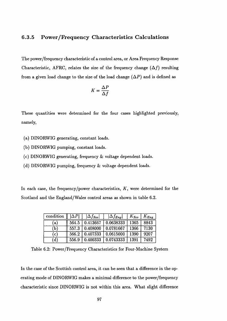
6.3.5 Pow er/Frequency Characteristics Calculations
The power/frequency characteristic of a control area, or Area Frequency Response
Characteristic, AFRC, relates the size of the frequency change (A /) resulting
from a given load change to the size of the load change (A P) and is defined as
A PK =
A /
These quantities were determined for the four cases highlighted previously,
namely,
(a) DINORWIG generating, constant loads.
(b) DINORWIG pumping, constant loads.
(c) DINORWIG generating, frequency Sz voltage dependent loads.
(d) DINORWIG pumping, frequency h voltage dependent loads.
In each case, the frequency/power characteristics, K , were determined for the
Scotland and the England/W ales control areas as shown in table 6.2.
condition |A P | \ A f s c o \ |A / e„ J K s c o A Eng
(a) 564.5 0.413667 0.0638333 1365 8843(b) 557.3 0.408000 0.0781667 1366 7130(c) 566.2 0.407333 0.0615000 1390 9207(d) 556.9 0.400333 0.0743333 1391 7492
Table 6.2: Power/Frequency Characteristics for Four-Machine System
In the case of the Scottish control area, it can be seen th a t a difference in the op
erating mode of DINORWIG makes a minimal difference to the power/frequency
characteristic since DINORWIG is not within this area. W hat slight difference
97
there is could be accounted for by the fact th a t the overall system operating con
ditions are slightly different when DINORWIG is pumping rather than generating
as is illustrated in the different A P figures which represent a difference in power
being exported from Scotland to England prior to the split.
The figures for the England/W ales area show a reduction in the power/frequency
characteristic when DINORWIG is pumping. This reflects the fact th a t there is
less regulation available in the system when DINORWIG cannot contribute to
the frequency control.
The figures for both areas show an increase in the power/frequency characteristic
when loads are frequency dependent. The load dependency is such th a t a reduc
tion in frequency causes a reduction in load. Consequently, in this case, the load
change caused in each area because of the split does not have as large an effect
as before and the generators are better able to cope with it.
6 .4 S tep Load C hange S tu d ies
A not too uncommon incident which any system frequency control must cope with
is the sudden loss of a generating unit. This results in an immediate step increase
in the load applied to the remaining generators. The response to this type of
incident was used to assess the relative performance of different system frequency
controllers. It was difficult to simulate the complete loss of a generator due to
the structure of the simulator. Consequently, these incidents were emulated by a
step increase in load at one of the system busbars.
98
6.4.1 Tests w ith D istributed Frequency R egulation
6.4.1.1 Sustained Fossil U nit Load Controllers w ith R ate Lim ited
Setpoints (5% M C R /m in). Dinorwig G enerating. Insensitive
Loads.
Figures 6.23(a)&;(b) show the response of the system when a step load change
of 500 MW (approx. 4% of to tal system load) was applied to busbar CEGB4.
Immediately, there is an imbalance between mechanical torque and electrical
load which results in the machines slowing down and a drop in frequency. The
frequency fall causes the turbine speed controllers of the fossil fired plant to
open their governor valves giving a surge in mechanical torque which initially
arrests the fall in frequency. Meanwhile, the unit load controllers s tart to reduce
the speeder m otor position, Zgvc, since the generation is now higher than the
setpoint. The action of the sustained load controller is to increase the setpoint
to compensate for the decrease in frequency. The speeder m otor position then
increases again until setpoint and generation settle out a t a level to correct the
frequency fall. During this run, DINORWIG was freely regulating and its output
increased accordingly to take a share of the higher load. The power on the
tie-lines between Scotland and England reflects the increased generation of the
SCOTLAND machines as this increase is being transferred to support the extra
load in England. The system frequency finally settles out with a steady-state
error of about 0.04 Hz.
99
6.4 .1 .2 Sustained Fossil U nit Load Controllers w ith R ate Lim ited
Setpoints (5% M C R /m in ). Dinorwig Pum ping. Insensitive
Loads.
The results of figures 6.24(a)&;(b) show the response to the same test as in sec
tion 6.4.1.1 (results in figure 6.23) when DINORWIG is not contributing to the
regulation. On comparison with figure 6.23, it is immediately apparent tha t the
control of frequency is not so good in a number of points: the size of the frequency
fall, the tim e taken to reach steady state and the steady state error. As before,
on the very initial fall in frequency, the governor valves of the fossil-fired units
open rapidly. However, in this test, this is not supported by extra generation
from DINORWIG and the frequency continues to fall faster than in the previous
test. The governor valves do not re-close as quickly as before and there is less of
a fall-off in mechanical torque and generated power. The system finally settles
with each fossil unit taking a larger share of the ex tra generation to make up for
the fact th a t there is no contribution from DINORWIG. It can also be seen tha t
the larger movements of the governor valves result in larger pressure deviations
and consequently larger changes in fuel input to correct these.
6.4 .1 .3 Sustained Fossil U nit Load Controllers w ith no Setpoint R ate
Lim its. D inorw ig Pum ping. Insensitive Loads.
The test of section 6.4.1.2 was repeated with no setpoint ra te limits in the fossil
unit load controllers. The results are shown in figures 6.25(a)&(b). Here it can be
seen th a t the frequency fall is arrested almost immediately by the initial opening
of the governor valves when the frequency drops. Because there is no ra te limit
on the setpoint, Lap, it quickly increases to correct the fall in frequency. This
100
means there is little error between the setpoint, L sp, and the generation, Pmw-> so
the stepper motor, Zgvc, is not moved in the opposite direction to the governor as
happened in the previous test. Thus the mechanical torque is not held back from
matching the electrical load and the system recovers very much more quickly.
6.4 .1 .4 N o Fossil U nit Load Controllers. D inorwig Pum ping. Insen
sitive Loads.
This test was performed to investigate the effect of the speed governor alone.
The results are shown in figures 6.26(a)&;(b). These show th a t it is indeed the
speed controller opening the governor in response to the initial drop in frequency
th a t causes the initial abrupt arrest of the fall. However, the longer term control
of frequency is not so tight as when the load controller also changes the speeder
m otor position to compensate for frequency error (compare with figures 6.24
and 6.25).
6.4.1.5 The Effect of U sing Oil-Fired Plant instead of Coal-Fired
Plant.
The results of section 6.4.1.2 were taken on a system where all of the fossil units
were coal-fired. This test was repeated using oil-fired units, all other conditions
being the same. The results are shown in figure 6.27. A comparison of figures 6.27
and 6.24 shows th a t the overall response of the two systems is very similar. The
only significant difference is in the effectiveness of the pressure control. The fuel
system of the oil-fired plant is more responsive than th a t of the coal-fired plant.
Consequently, a tighter control can be kept on superheater outlet pressure, P2 , by
101
varying the fuel flow, M ju. This of itself does not improve the output performance
in respect of frequency regulation. However, it has already been seen th a t a
m ajor lim itation on the performance in respect of frequency regulation is the rate
limit of the generation setpoint, L sp. (Compare the results of sections 6.4.1.2
and 6.4.1.3.) The reason for imposing a rate limit on the setpoint, T ,p, is to
minimise the pressure excursions on changing load. It can be concluded th a t
with the tighter pressure control obtainable with oil-fired plant, a higher setpoint
ra te limit could be tolerated before the size of the pressure excursions on load
changes were unreasonable.
6.4.1.6 The Effect of Setpoint R ate Lim its
It could be noted from the results so far in this section th a t the setpoint rate
limit has very little effect on the quality of pressure control (compare P2 in fig
ures 6.24(b) and 6.25(b)). Based on these results it might be argued th a t there is
no need for a setpoint rate limit at all. To investigate the effect of setpoint rate
limits further, tests were carried out to simulate scheduled load changes rather
than those forced by frequency regulation.
Figures 6.28(a)&(b) and 6.29(a)&(b) are the results of applying a change in load
demand to the CEGB and SCOTLAND machines when they are operating in a
sustained load control mode. Figure 6.28 shows the results when the setpoints,
L ap, are rate lim ited by 5% M CR/m in and 6.29 shows the results with no setpoint
ra te limits.
The setpoint rate lim it can be clearly seen in L sp in figure 6.28(a). To m aintain
the load/generation balance, an increase of 500 MW by the twenty-one CEGB m a
102

chines has been offset by a decrease of 500 MW in the five SCOTLAND machines.
Each individual machine has its setpoint, L sp, rate limited to 5% M CR/m in. Con
sequently, each CEGB machine requires an increase of about 22 MW whereas each
SCOTLAND machine needs to decrease its output by 100 MW. At the same ram p
rate, the SCOTLAND machines will take longer for the setpoint, L ap, to reach
the desired value, Ldv
Initially, both the CEGB and SCOTLAND machines s tart to follow a setpoint
ramping at its rate limit towards the desired value. Because there are more CEGB
machines than SCOTLAND machines, their combined effect is to increase to tal
CEGB generation faster than the SCOTLAND generation is decreasing and so
the system frequency rises. The NWALES machine is also regulating, though
not changing its generation desired value, and its setpoint, L sp, decreases to help
offset the increase in frequency. The ramping up of the CEGB setpoint reverses
to also offset the increase in frequency. Having arrested the rise in frequency, the
rate limit on the fall of power from SCOTLAND, through the effect on frequency,
forces the CEGB machines to ram p to their final output at a slower rate. The
NWALES machine is also able to increase its output back to its desired value.
The effect of these power changes on the superheater output pressures can clearly
be seen in P2 .
In figure 6.29(a), the load setpoints, L sp, are not rate limited when they follow
the change in Ldv• In this case, there is only a slight imbalance between the
CEGB increase in power and the SCOTLAND decrease. Consequently, there is a
much smaller change in frequency. In this case, frequency tends to fall and then
recover, ra ther than rise as in the previous situation. The limiting factor on the
ra te of change of generation is now the dynamics of the generating units which
will be slightly different because of the different operating points of the CEGB
103
and SCOTLAND machines. As before, the NWALES generation also changes
in response to the frequency deviation. However, a comparison of the resulting
pressure deviations, P2, dem onstrates how much more seriously this control is
affected by the actions of the load control when no setpoint rate limit is used.
Hence the use of a rate limit on the load setpoint, L sp.
6.4 .1 .7 The Effect o f Frequency and Voltage D ependent Loads
The test of section 6.4.1.1 (with results shown in figure 6.23) was repeated on a
system with loads sensitive to frequency and voltage. These results are shown
in figures 6.30(a)&;(b). The load dependency is such tha t the overall effect of a
reduction in system frequency is to also reduce the to tal system load (a rule-of-
thum b figure is often quoted as 2% of total load per Hertz). Hence, on the sudden
increase in load, the resulting fall in frequency actually reduces the effective load
and consequently the frequency does not fall as far as it would have done if the
load were insensitive to frequency. This effect can clearly be seen in a comparison
of the frequencies in figures 6.23(a) and 6.30(a). The resulting transient changes
in torque and generation are also slightly reduced since the frequency deviation is
smaller. However, the final values of generation are the same as before since the
frequency has returned to near its original value and so the same to tal increase
in generation needs to be provided to m atch the imposed increase in load.
An equivalent Area Control Error has been included with the results of this last
test so th a t it may be compared with those th a t follow. This ACE did not
occur in practice since Autom atic Generation Control was not running, but was
calculated from the frequency and tie-line power data as if the standard AGC
were running as described in the next section.
104
6.4.2 Tests w ith Centralised A utom atic G eneration Controllers
A utom atic Generation Control (AGC) was applied to the simulation as described
in section 3.5.3. Initially, a flat-frequency control mode was applied to compare
the results with those of the distributed controllers and then frequency-bias mode
was implemented to also control the tie-line power. The Area Frequency Response
Characteristics, or power/frequency characteristics, used were those calculated in
section 6.3.5. The AGC gains, Tn and Cp in equation 3.1, were initially selected
as 65 and 0.2 respectively, these being the average of values specified by Glavitsch
and Stoffel in [18] (see discussion on page 22).
6 .4 .2 .1 F la t F re q u e n c y M o d e A G C . D in o rw ig G e n e ra tin g . F req u e n c y
a n d V o ltag e S en sitiv e L oads.
The results of this test are shown in figures 6.31(a)&(b). The conditions of the
test were similar to those of section 6.4.1.7 (with results in figure 6.30), except
th a t, rather than frequency regulation being performed by the sustained fossil
unit load controllers, in this case, frequency regulation was performed for each
control area by the AGC algorithm. The fossil unit load controllers then acted
in a non-sustained mode to follow the desired values set by the AGC.
It can be seen from figure 6.31(a) tha t frequency takes longer to come to a steady
state since the frequency transient has continued to rise to completely correct
the error. The very initial torque and generation transients are similar to the
non-AGC case which is because this part of the response is due to the turbine
speed governors as discussed in section 6.4.1.4. The medium term response of the
fossil units is still dictated somewhat by the rate limit on the setpoints. However,
105
the AGC algorithm shares the total extra required generation between all of the
fossil units and their final levels of generation are sufficient to make up the whole
increase in load. In this case, DINORWIG is not part of the AGC algorithm. Con
sequently, having reacted to the initial frequency error through governor action,
its generation gradually returns to its original level as the frequency returns to
its setpoint. The power being transferred on the tie-lines illustrates the increased
contribution th a t the Scottish machines are making, now th a t DINORWIG has
no steady state increase in its generation.
6 .4 .2 .2 T ie -L in e B ias M o d e A G C . D in o rw ig G e n e ra tin g . F req u e n c y
a n d V o ltag e S en sitiv e L oads.
Figures 6.32(a)&(b) and 6.33(a)&(b) illustrate the response of the system when
the AGC is in tie-line bias mode. In this mode, the tie-line power is also regu
lated. By comparing these results with those of the previous section (shown in
figure 6.31) it can be seen tha t the frequency response is very similar, but the
tie-line power now returns to its initial value. By controlling the tie-line power,
the AGC ensures tha t the load increase is matched by an increase in generation
only from the area in which it occurred. The generation results show how the
SCOTLAND generation is returned to its previous value while the CEGB and
NWALES machines pick up all of the extra load between themselves.
6.4.3 T he Effect of the AGC Frequency Bias Param eter B
Ordinarily, AGC is implemented with the frequency bias, B , (relating frequency
to power in forming the Area Control Error, equation 3.2) set equal to the Area
106
Frequency Response Characteristic. It has been suggested [27] th a t it might be
preferable to operate with B set to half the value of the AFRC. Several simulation
runs were performed to investigate the effect of the param eter B.
Figures 6.34(a)&(b) show the results of the same test as before but with half the
value of B for the England/W ales area. Figures 6.35(a)&(b) show the results
when B is twice the value of the AFRC. Comparing these with the results for B
equal to the AFRC (figures 6.32 and 6.33), the effect on the CEGB Area Control
Error can clearly be seen where it incorporates a lesser and a greater contribution
from the frequency error. However, the result of this on the frequency and tie-
line power responses is not nearly so marked. From the frequency graphs in
figures 6.33(a), 6.34(a) and 6.35(a), a slight increase in speed with increasing
value of B can be observed. However, the differences are not large and it would
appear th a t the rate limit on the fossil unit setpoints prevents an increase in the
speed of response of the generation as the Area Control Error gets larger with
increasing B . In order to investigate just the effect of the controller, the tests
were repeated with no setpoint ra te limits and with DINORWIG pumping so tha t
it had no effect on the regulation.
The unlim ited results are shown in figures 6.36(a)&(b), 6.37(a)&(b) and 6.38(a)&
(b) for B of the CEGB control area equal to AFRC, half AFRC and twice AFRC,
respectively. The effect of changing B is now very obvious. As the value of B
increases, the tim e taken for the Area Control Error to come to zero decreases.
W ith both the high and low values of B , there is more overshoot in the frequency
response than when B is set to the value of the AFRC. The faster control available
from using a higher value of B results in less disturbance to the superheater
pressure control in the other area and, conversely, a low value of B results in a
greater disturbance. This may be explained by observing th a t with a lower value
107
of B , the local area controller is less reactive to frequency deviations and does not
try so hard to correct them . The persisting errors cause the other area controller
to demand more regulation from its generators. Consequently, a low value of B
in just one area causes the other area to perform more regulation even when the
disturbance is not in the other area.
The results were also repeated with the B values in both area controllers set to
half of their respective AFRCs. These are shown in figures 6.39(a)&;(b). Here the
response is slow as before. However, the effect on the pressure control of both
areas is similar illustrating how they are taking a similar share of the regulation
when compared to the case when both B s are set equal to the AFRCs. Hence,
the practice of setting all area controllers to have B equal to th a t area’s AFRC
ensures some level of “fairness” in the regulating duties of the different areas,
even though the ultim ate correction of ACE to zero is assured for whatever value
of B.
None of these effects is very obvious when the speed of response of the generating
units is dominated by the load setpoint rate limits. Consequently, the relatively
small differences in AFRC calculated in section 6.3.5 for different system operat
ing conditions were not taken into account in the results of this chapter and all
AGC controllers used the same param eter values. This insensitivity in the pres
ence of rate limits may suggest th a t in an area dominated by slow, rate limited
units the value of B may not need to be changed with different operating con
ditions, resulting in a simpler controller. However, the effect of system loading
must also be considered (see later in section 6.4.7.2).
108
6.4.4 T he Effect o f AGC Controller Gains Tn and Cp
A sequence of runs was performed varying the AGC controller gains Tn and Cp.
In all instances, the controllers for the two areas, Scotland and England/W ales,
were the same. The base case was taken as th a t described in section 6.4.2.2
where, for both areas, Tn = 65 seconds and Cp = 0.2.
6 .4 .4 .1 T h e E ffec t o f Tn
Figures 6.40(a)&(b) show the results with Tn increased to 100 seconds, while
figures 6.41(a)&(b) were obtained with Tn = 30 seconds. These may be com
pared with the nominal case of Tn = 65 seconds shown to the same scale in
figures 6.33(a)&(b). The frequencies in figure 6.41(a) show an obviously un
derdam ped response for the shorter Tn, corresponding to a higher gain for the
integral term of the controller. The frequencies in figure 6.40(a) for Tn = 100
seconds are the most dam ped as would be expected. However, the response in
this case has been slowed down slightly by the increased damping. This is best
seen in the Zgv/ Z gvc trace where it can be surmised tha t the frequency error is
zero when Zgvc meets Zgv. For the results, this tim e can be seen to be shortest
for the middling value of Tn = 65 seconds (figure 6.33).
6 .4 .4 .2 T h e E ffec t o f Cp
Figures 6.42(a)&(b) and 6.43(a)&(b) show the results with Cp = 0.1 and Cp = 0.3
respectively. Again, these may be compared with the nominal case shown in
figure 6.33 where Cp = 0.2. A comparison of these three figures would suggest
109
th a t a low value of Cp produces a slower, less well damped response as is seen
in figure 6.42(a). The results of figure 6.43(a) would suggest th a t a higher value
of Cp would be most desirable to produce the fastest and best dam ped response.
However, the comparison may be clouded a little because of the contribution from
DINORWIG. The tim e taken for the DINORWIG generation to finally return to
its initial value is very similar in all three cases. However, with the higher values
of Cp, DINORWIG generation is on average higher during its transient increase
from its steady state level. In other words, the integral of DINORWIG Pmw is
higher for higher Cp. This relates to energy and consequently water usage and
so the final choice of Cp may be based on making a compromise between the
dam ping of the frequency transient and the use of hydro plant in helping the
regulation.
6 .4 .4 .3 C h o ice o f O p tim a l V alues fo r Tn a n d Cp
The results of this section would suggest tha t the most appropriate values for
Tn and Cp lie well within the range of those in use for other systems [18]. A
common approach to this type of problem is to minimise some cost function
with respect to the controller gains. The simulation may be used to perform a
series of tests with Tn and Cp taking different values within the range already
identified as being appropriate. The choice of the “best” values for the gains will
be based on a comparison of several factors such as speed of response, control
effort, contribution from hydro units and damping of response. These factors
may be used to formulate a cost function for each set of Tn/Cp values. Among
the simplest cost functions which may be used are JACE and JA C E 2 though
these may not take into account all of the significant factors. P lotting the cost
function against Tn and Cp at several different values would enable the gains
110
which minimise the cost function to be estimated.
6.4.5 A N ew A rea Control Error
The new Area Control Error (ACE) proposed by M.L.Kothari et al. in [40],
given in equation 3.2, was implemented in the AGC code. A controller using
this error always guarantees zero steady state tim e error and inadvertent energy
interchange, unlike conventional ACE controllers (see discussion on page 26).
This was initially implemented with a gain on J A C E of a = 0.01 as suggested
in [40].
The previous step load change test was repeated with the new ACE. The results
are given in figures 6.44(a)&(b). Comparing these with the results of the similar
controller using a conventional ACE given in figure 6.33, it can be seen th a t it
takes longer for both the frequency and the tie-line power to settle. However,
the integral of frequency error is brought to zero by the end of the transient by
forcing the frequency to remain high for a while after the initial fall. This ensures
th a t the tim e error introduced by the initial error in frequency is reduced to zero.
Similar comments can be made with regard to the tie-line power. The integral
of tie-line power error which is inadvertent energy interchange, is also reduced to
zero by the tim e the system comes back to steady state.
6.4.5.1 The Effect o f the Integral Gain a
Two further runs were carried out with a = 0.02 and a = 0.005, the results of
which are shown in figures 6.45(a)&(b) and 6.46(a)&(b) respectively. These may
111
be compared with the results of the previous run with a = 0.01 as shown in
figure 6.44. In figure 6.45 the controller tries to correct the integral error more
severely by, for example, allowing the frequency to rise higher to correct the
integral error from the initial fall more quickly. However, this leads to a rather
oscillatory response with rather large overswings. This also has a larger effect on
the excursions of superheater pressures. Making the gain a smaller as shown in
figure 6.46 produces a rather more gentle control action which nonetheless finally
reduces the integral of frequency and tie-line power error to zero. The final choice
of a would have to be a compromise between speed of response and severity of
control action. However, it would appear th a t a need not be very large.
6.4.6 T he Effect o f Controller Interval
The implementation of the AGC controller used in these studies was of a discrete
kind with an associated control interval time. In all the runs so far discussed,
this interval was five seconds. Five seconds had been chosen since this was gen
erally the shortest interval considered for real controllers in the literature (see
section 3.4). Many theoretical papers use a control interval of two seconds (see
section 3.3), however, the results here would suggest tha t five seconds is perfectly
adequate. A longer interval still may be more desirable from the point of view
of practical implementation, hence the effect on the quality of control of using
longer control intervals was investigated. The m ajor disadvantage of a long con
trol interval is th a t if an event occurs on the system immediately after one control
action, this will not be acted upon by the controller until another whole control
interval has elapsed. In the case of a sudden fall in frequency due to, say, the
loss of a generator, in the case of a long control interval the frequency will have
fallen further before corrective action is taken than in the case of a shorter con
112
trol interval. Even if there is no delay in noticing the frequency fall, performance
deteriorates with increasing control interval, a feature which is worsened with the
use of ra te limited setpoints. These points are illustrated in the following results.
The results of figure 6.44 may be taken as the base case. Here, the controller
interval was 5 seconds and the fall in frequency was noticed immediately. Fig
ures 6.47(a)&(b) show the corresponding case when the AGC controller does not
react until a whole control interval, ie. five seconds, after the initial frequency
drop. In the second case where there is a delay in the controller response, the
frequency falls very slightly further and its fall is arrested very slightly later.
However, the overall responses and recovery times are very similar.
Figures 6.48(a)&;(b) and 6.49(a)&(b) show the responses when the control interval
is ten seconds, figure 6.48 with no delay, figure 6.49 with a delay of one control
interval, ie. ten seconds. On comparing one with the other, the effect of the
delay with this interval is more obvious. W ith the delay, the frequency falls
further before being arrested. This then results in a slightly larger overshoot
on recovery as the controller attem pts to correct for tim e error, ie. integral of
frequency error. The delay is obvious in the CEGB Pmw/Ldv/Lap trace. In the
first case, Ldv changes and L ap starts to change at the same tim e as the governor
speed controller opens the governor valve and causes the initial surge in power.
In the second case, the setpoints do not s tart to change until after the speed
governor action. Consequently, considering the England/W ales subsystem, the
load controllers decrease the speeder motor positions, Zgvc, further than in the
previous case since the lagging change in setpoints means there is a larger load
error (L ap — Pmw). All in all, this results in a delay in recovering the frequency
error.
113
On comparing the ten-second results with the five-second results, with no delays,
ie. figures 6.48 and 6.44, it can be seen th a t the longer control interval results
in a slightly more oscillatory frequency response and a larger tie-line power error
with consequently larger corrections to bring the integral of tie-line power error,
ie. inadvertent energy interchange, to zero.
Figures 6.50(a)&;(b) and 6.51(a)&(b) show the responses when the control interval
is fifteen seconds, again with no delay (figure 6.50) and w ith delay (figure 6.51).
W ith the longer control interval, the response is now obviously more oscillatory.
Again, the frequency fall is larger when there is a delay before the controller
reacts causing larger overshoots and a slightly longer settling time.
Increasing the control interval too far results in limit cycling, or even an unstable
response, as shown in figures 6.52(a)&(b) and 6.53(a)&(b) where the control
interval is twenty seconds.
As has been noted previously, the rate limit imposed on the fossil unit load con
trollers setpoints, L ap, has a detrim ental effect on the quality of load-frequency
control. This effect exacerbates the worsening response th a t is obtained as the
controller interval is lengthened. To dem onstrate this, the fifteen-second con
troller responses (shown in figures 6.50 and 6.51) were repeated w ithout setpoint
rate limits. These results are shown in figures 6.54(a)&(b) and 6.55(a)&(b) (im
mediate reaction to frequency fall and delayed reaction respectively). W ithout the
rate limits, the response is very much less oscillatory and the differences in speed
with which the frequency fall is arrested is more obvious. Figures 6.56(a)&(b)
show the base case (ie. five-second controller) when there are no ra te limits. As
would be expected, this shows a tighter control than the corresponding rate lim
ited case (shown in figure 6.44). Comparing the five-second and fifteen-second
114
controllers without rate limits (figures 6.56 and 6.54 respectively) it can be seen
tha t there is still some reduction in quality of control with the longer interval in
tha t there is a slightly more oscillatory response with larger overshoots. As seen
before in the rate limited case, the effect of a delay in noticing the frequency fall
produces an obviously worse result as shown in figure 6.55.
6.4/7 Effects o f System O perating Conditions
6.4.7.1 The Effect of M achine Loading
The standard step load change test was applied to a system in which the indi
vidual generators were more heavily loaded than in previous runs. The standard
AGC was used as in section 6.4.5 (with results in figure 6.44). This was achieved
by using twenty instead of twenty-one generators in the CEGB group, and four
instead of five in the SCOTLAND group. The results of this test are shown in
figures 6.57(a)&(b).
A comparison of the frequency traces in figures 6.44(a) and 6.57(a) shows tha t
the frequency falls further before being arrested in the case of the more heavily
loaded machines. The initial “blip” in the frequency trace due to the first abrupt
opening of the governor valves is also lower. There are differences, too, in the
tie-line power traces. W ith heavily loaded units there is not such a high surge in
tie-line power resulting from the initial fall in frequency. This reflects the changes
in generation of the SCOTLAND units. The reason for these differences is the
deteriorating responsiveness of the generating units as they are operated with the
governor valves further open. This is due to the non-linear characteristic of the
governor valves relating steam flow to valve opening. The reduced regulation of
115

the fossil units is also reflected in the DINORWIG generation where, in the case
of more heavily loaded fossil units, DINORWIG takes on a larger share of the
regulation.
The non-linear effect of the valves may be illustrated by considering the governor
valve movements of figures 6.44(b) and 6.57(b). The size of the initial opening of
both the CEGB and SCOTLAND units is larger in the case of more heavily loaded
machines (figure 6.57) as would be expected from the larger fall in frequency.
However, under these operating conditions, this does not result in a larger increase
in power in the SCOTLAND machines. Rather, because of the valve non-linearity,
a smaller power change results even from this larger movement of the valve. In
the case of the CEGB units, a larger movement of the governor valves results in
a similar power increase compared to the less heavily loaded condition. In fact,
the difference in operating points between the two sets of results is greater for
the SCOTLAND group than for the CEGB group.
6.4.7.2 The Effect of Network Loading
The standard step load change test was also applied to a system with twice the
load of the previous runs. The numbers of generators in each group was dou
bled in order th a t each individual generator should be operating under the same
conditions as before. The results of this test are shown in figures 6.58(a)&(b).
From a comparison of figures 6.58 and 6.44 it can be seen tha t the 500 MW step
load change results in a lower fall of frequency in the more heavily loaded network.
This is to be expected since, in this case, the load change relative to the to tal
load is only half tha t of the previous case. So, in this respect, a generation loss
116
of a given size will be less severe in a system which has a larger to tal load.
There is another significant difference between the results in figures 6.58 and 6.44.
The response of the more heavily loaded case is rather slower and more oscillatory.
On inspection of the generation curves of the fossil units in figure 6.58(a), it can
be seen th a t the setpoints are not rate limited for all but the first few seconds of
the response. This, then, reflects a condition similar to th a t shown in figure 6.38
and discussed in section 6.4.3 where the value of the ACE param eter B was only
half the value of the AFRC. In changing the conditions of the system such th a t
there are now twice as many generators regulating than previously, it m ight be
reasonable to assume th a t the AFRC is also doubled. From figure 6.58(a) it can
be seen th a t in this particular case the response is no longer dom inated by the
setpoint ra te limits. In order to improve the response, a better value of B would
need to be used in the calculation of the Area Control Errors. This would suggest
th a t in a system where AGC is required to operate over a fairly wide range of
loading conditions, a constant value of B may not be appropriate unless it is such
th a t the response is actually dominated by the setpoint rate limits over the full
load range.
6.5 S u m m ary
A large num ber of results have been presented in this chapter and this section
has been included in order to clarify the outcome of this work.
In summary, then, the following proposals are made with regard to the control
of the British power system:
117

1. Operate the complete system as two distinct control areas, England/W ales
and Scotland, so th a t the power on the tie-lines between the two may be
regulated and each area will make up for its own losses in generation whilst
maintaining frequency at the setpoint.
2. W ithin each control area, implement a centralised form of load-frequency
control to give zero steady state frequency errors and to enable the tie-line
power to be taken into account.
3. Use a form of area control error (ACE) which incorporates the integrals
of frequency and tie-line power as well as the frequency and tie-line power
themselves, in order to be able to autom atically reduce time error and
inadvertent energy interchange to zero.
4. Set the ACE frequency bias param eter, B , to the Area Frequency Response
Characteristic (AFRC) in both areas to ensure fairness of regulating duties
between the two areas. The value of B has some effect on the speed of
response of the controller. However, fairness will only be ensured if the B s
of both areas are set according to the same criteria.
5. Use middling values of the controller gains, Tn = 65 and Cp = 0.2, which
would appear to be adequate in the first instance. However, further simu
lation and analysis could be performed to choose more optim al values.
6. W ith regard to the gain on the integrals of frequency and tie-line power,
use the value of a = 0.01 recommended in the literature. It would appear
tha t the value of a is not very critical and may be quite small. The final
choice would depend on the timescale over which it is intended th a t tim e
error and inadvertent energy interchange be corrected.
7. Use a controller interval of five seconds. There is little point in operating
very much faster than this because of the typical value of intervals used
118

by generating unit load controllers. A slower rate may be desirable from
an implementation point of view. However, long intervals may lead to
instability and these initial results suggest an interval no slower than once
every ten seconds should be used.
The following chapter presents results from the more complex 25-machine study
in order to illustrate a few points th a t could not be dem onstrated in the 4-machine
study. However, this adds little to the proposals listed above, but does point to
some further issues which would need to be taken into account in an operational
system.
119
C hapter 7
T w enty-F ive M achine Studies
Although most of the significant properties of centralised load/frequency control
were illustrated by the four-machine studies discussed in chapter 6, it was nec
essary to model a more complex system in order to dem onstrate certain other
characteristics. This model consisted of a to tal of twenty-five generating groups,
six of which modelled each Dinorwig unit independently, and sixty load groups.
This level of complexity allowed a more realistic mix of plant to be modelled, for
example, by allowing the six Dinorwig units to act independently. It also allowed
for the regulation to be performed by a smaller proportion of the generators than
could be implemented on the fairly crude four machine system.
7.1 S y stem Sp lit T est
As with the four machine system, the initial test to be performed was a system
split disconnecting Scotland and England. The resultant trends are shown in fig
ures 7.1(a)-(e). For this test, all hydro units, including the six units a t Dinorwig,
were pumping.
120
Considering first the generators in Scotland (results are shown for LONGANNET,
HUNTERSTN and PETERHEAD), immediately the tie-lines are broken, the
electrical load on each of these machines falls abruptly by around 100 MW. This
relates to the to tal load lost of approximately 609 MW shared between the six
therm al units and the hydro units at FOYERS and CRUACHAN (not shown).
The load control on the therm al units is such th a t LONGANNET (Coal-fired)
is operating in a sustained load control mode whereby its load setpoint, L ap,
varies from the desired value, in order to help correct frequency errors. The
other units, HUNTERSTN and PETERHEAD, are nuclear and as such do not
regulate with respect to frequency except through their speed governors. For all
but severe frequency errors, the governor droop, or gain between frequency error
and offset of Zgv, the governor valve position, from Zgvc, its nominal position
set by the speeder motor, is such as to be less sensitive in nuclear units than
in fossil units. This can be illustrated by considering the Governor graphs for
LONGANNET and HUNTERSTN given in figure 7.1(d). For the initial rise
in Scotland frequency, f acoy of about 0.9 Hz, the LONGANNET governor valve
closes by about 0.45 pu. whereas the HUNTERSTN governor moves only about
0.1 pu. Because of the non-sustained response of the nuclear units, the load
setpoints, L ap, remain constant. Consequently, the speeder motor position, Zgvc,
is increased in an a ttem pt to bring the generation, Pmw, back to meet the setpoint,
L sp. At the same tim e, the LONGANNET setpoint is decreasing in response to
the high frequency and the LONGANNET generation remains low. In fact, the
LONGANNET generation continues to decrease which allows the generation in
the nuclear units to increase again to their setpoints. The Scotland system finally
settles with all the decrease in load being taken by the LONGANNET units, and
the frequency constant at about 50.8 Hz.
The situation in the England/W ales subsystem is the opposite to th a t in Scotland.
121
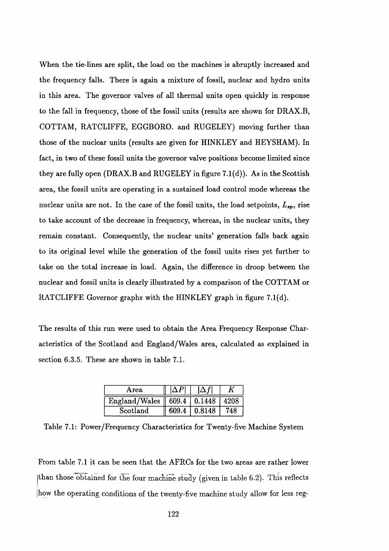
W hen the tie-lines are split, the load on the machines is abruptly increased and
the frequency falls. There is again a m ixture of fossil, nuclear and hydro units
in this area. The governor valves of all therm al units open quickly in response
to the fall in frequency, those of the fossil units (results are shown for DRAX.B,
COTTAM , RATCLIFFE, EGGBORO. and RUGELEY) moving further than
those of the nuclear units (results are given for HINKLEY and HEYSHAM). In
fact, in two of these fossil units the governor valve positions become limited since
they are fully open (DRAX.B and RUGELEY in figure 7.1(d)). As in the Scottish
area, the fossil units are operating in a sustained load control mode whereas the
nuclear units are not. In the case of the fossil units, the load setpoints, L ap, rise
to take account of the decrease in frequency, whereas, in the nuclear units, they
remain constant. Consequently, the nuclear un its’ generation falls back again
to its original level while the generation of the fossil units rises yet further to
take on the to ta l increase in load. Again, the difference in droop between the
nuclear and fossil units is clearly illustrated by a comparison of the COTTAM or
RATCLIFFE Governor graphs with the HINKLEY graph in figure 7.1(d).
The results of this run were used to obtain the Area Frequency Response Char
acteristics of the Scotland and England/W ales area, calculated as explained in
section 6.3.5. These are shown in table 7.1.
Area |A P | |A / | KEngland/W ales 609.4 0.1448 4208
Scotland 609.4 0.8148 748
Table 7.1: Power/Frequency Characteristics for Twenty-five Machine System
From table 7.1 it can be seen tha t the AFRCs for the two areas are rather lower
than those obtained for the four machine study (given in table 6.2). This reflects
how the operating conditions of the twenty-five machine study allow for less reg
122
ulation than under the conditions of the four machine study. There are a number
of reasons for this. The operating conditions of the twenty-five machines study
were set up to model a summer night tim e loading condition. In this situation,
the load on the network is low and there is also a relatively high proportion of
unresponsive generation such as the nuclear units whose generation is not re
duced during the night. As small a number of fossil units as possible will be run
with consequently a number of these generating near their maximum. Finally,
pum ped-storage units will be pumping rather than generating during the night
and so will not be contributing to frequency regulation. Consequently, this is a
scenario which represents a worst case situation for load/frequency control.
7.2 S tep Load C hange S tu d ies
Similar step load change tests to those of chapter 6 were performed on the twenty-
five machine system. These consisted of a step load change of 500 MW at busbar
EGGB4J while an AGC controller was running in tie-line bias mode with the
controller param eters Tn and Cv set to 65 and 0.2 respectively in both areas. The
controllers used the Area Control Error investigated in section 6.4.5. Initially,
all hydro units were pumping and all fossil unit setpoints were rate limited to
5% M CR/m in.
The results of the first test are shown in figures 7.2(a)-(e). The response is
poor, allowing the frequency to fall by nearly 0.5 Hz and resulting in a very
underdam ped recovery. This is as a result of the small am ount of regulation
available as explained in section 7.1. There is only a small assistance to frequency
regulation from the nuclear units, HUNTERSTN, HINKLEY, PETERHEAD and
HEYSHAM, whose governor valves do not move far from their nominal positions
123
because of their high droop. The response to the load change is also hindered
by the fact th a t several fossil units do not make as much of a contribution as
they might because they are limited at or near maximum output: DRAX.B,
EGGBORO. and RUGELEY. In addition to this, there is the slugging of the
response due to the ra te limits on the power setpoints compounded by the fact
th a t those units near their maximum limits are unable to follow the setpoint
changes. The response is also degraded by the fact th a t there is no contribution
from the hydro units. In fact, this response is rather unrealistic since such a large
fall in frequency as seen here would, in reality, cause autom atic cutting in of some
hydro units. This action is investigated later in section 7.2.3.
7.2.1 M ore Effective R egulation
The previous test was repeated with two Dinorwig units generating, and regulat
ing, instead of pumping. To counterbalance this extra generation, the generation
levels of some other units were reduced. The results of this test are shown in
figures 7.3(a)-(e).
W ith the two Dinorwig units helping with the regulation, the response to the
step change in load is altogether more stable. The frequency does not fall as far
before being arrested and there are no oscillations on recovery. It can be seen
from the generation traces tha t while the faster hydro units arrest the fall in
frequency, the slower fossil units in England and Wales follow their rate limited
setpoints to eventually take up all of the change in load. The Scottish generation
(LONGANNET) increases initially to help offset the fall in frequency, but, as
frequency recovers, it is reduced to bring the tie-line power back to zero. In
deed, the Scottish generation is low for a while in order to reduce the integral
124
of the ACE and hence the tim e error and inadvertent energy interchange on the
tie-lines to zero as illustrated in figure 7.3(e). A clear distinction can also be
seen between the regulating fossil units and the non-regulating nuclear units in
figure 7.3(b). In fact, now th a t the control of frequency is improved, there is very
much less disturbance to the nuclear generators as compared to the previous sit
uation (compare figure 7.3(b) with figure 7.2(b)). The dominance of the setpoint
ra te limits in the fossil units is also clearly illustrated in figures 7.2(a) & (b).
7.2.2 T he Effect o f Different Setpoint R ate Lim its
The step load change test was again repeated. In this instance, several of the Eng
land/W ales units had their setpoint rate limits increased from 5% M C R /m in to
10% M CR/m in. The results of this test are shown in figures 7.4(a)-(e). Again,
there is an improvement in the regulation of the frequency and tie-line power
when compared with the previous test. The excursions of frequency and tie-line
power are not so large and the errors are reduced to zero more quickly. This
is due to the greater regulation now being performed by the faster fossil-fired
units. The difference in response between slow and fast units can be seen from
a comparison of the COTTAM and RATCLIFFE or EGGBORO. and RUGE
LEY Generations in figure 7.4(b). Because the units with the faster setpoint
ram ps (COTTAM and EGGBORO.) increase their generation more quickly they
finally take up a larger share of the increased load than do the slower units (RAT
CLIFFE and RUGELEY). Although this increase in responsiveness of some fossil
units has reduced the regulating requirements of the DINORWIG units (compare
figures 7.4(a) and 7.3(a)), and the impact of the disturbance on the nuclear units,
there is now, in fact, a level of “unfairness” between the regulating duties of the
slow and fast fossil units. It may be acceptable to allow the faster units to take
125
on a greater share of the regulation. Then again, from an economic viewpoint, it
m ight be more desirable th a t in the longer term , the slower units finally take on a
greater share of the load thus allowing the faster units to reduce generation again
back towards their economic levels. This requires a more sophisticated AGC al
gorithm which splits the generation setpoints into two components for economic
operation and load/frequency regulation. This im portant aspect of AGC is not
considered here but would be a significant further development to these studies.
7.2.3 T he U se o f Low Frequency Relays on Hydro Plant
As previously mentioned, it is common practice for hydro units such as those at
Dinorwig to operate in a mode whereby on an excessively low frequency their out
put is rapidly increased to maximum. Such a mode of operation was incorporated
into the model of the Dinorwig units. The step load change test was repeated
w ith DINORWIG1 having a Low Frequency Relay (LFR) setting of 49.85 Hz and
a dead tim e of 2.75 seconds. This m eant th a t the relay would operate if the
frequency had been below 49.85 Hz for more than 2.75 seconds. It would then
take a Dinorwig unit about ten seconds to change from full pumping to maximum
generation. The simulation results of this situation are given in figures 7.5(a)-(e).
The rapid rise in the DINORWIG 1 generation is clearly shown in figure 7.5(a).
Initially, DIN0RW IG1 generation starts to rise through normal governor action
as before but then, once the LFR has responded, the generation quickly rises to
its maximum. The effect of this is to arrest the fall in frequency rather sooner
than in the previous tests. The recovery of frequency and tie-line power to their
original values is faster. The reaction from other regulating units is smaller than
in the previous case since DIN0RW IG1 has taken a significant portion of the
126

increase in load (about 200 MW of the 500 MW change). W ith the frequency fall
having been arrested by the rise in generation from DINORWIG1, on a longer
timescale, the AGC varies the generations of the other units to bring the steady
sta te values of Area Control Error and its integral to zero.
127
C hapter 8
C onclusions
A com puter simulation has been set up which is suitable for the study of Au
tom atic G eneration Control on the British power grid. This has entailed the
incorporation of more detailed model units into a pre-existing electro-mechanical
power system sim ulator at the University of Bath. This simulation has been
used in a prelim inary study of centralised load/frequency control which could be
used to replace the current distributed type of control and amalgamated with
economic dispatch calculations to provide Autom atic Generation Control.
Models of the order of ten to twenty states of fossil-fired generation units and
hydro units have been implemented and incorporated into the existing power
system sim ulator. Nuclear units were modelled as unresponsive, high droop,
fossil units. The hydro model also included the response of low frequency relays.
These models were validated by comparison with results from the original models
from which they were taken and, to an extent, with real plant data where this
was available. Models were also implemented of loads sensitive to frequency and
voltage variation.
The im plem entation of the fossil-fired unit models also required the development
128
of controllers to control the power generation and the steam pressure of the boiler.
This was designed as a traditional Boiler-Follows-Turbine (BFT) control whereby
two independent controllers were implemented, one controlling power output by
varying the nominal position of the governor valve set by the speeder motor
position and the other regulating steam pressure by varying fuel flow into the
boiler. The structure and gains of an operational controller were available and
this was also implemented. This was a multi-variable controller which had been
designed for one particular plant via a discrete “black-box modelling” approach
to p lant identification and controller design. Although this controlled the boiler
model very well under some conditions it was found not to be robust for the
range of plants th a t were required to be modelled. Consequently, it was found
more successful to use the cruder, but more flexible and more readily tunable
B FT design.
In order to design for the BFT control, it was necessary to produce a linear
model of the plant from the non-linear model used for the simulation. This was
perform ed with the assistance of a symbolic m athem atics program to produce
simplified th ird order linear models for the two sections of plant to be controlled.
This then enabled simple Proportional-Integral and Integral controllers to be
designed for the pressure and load loops.
The simulation was used to investigate the operation of load/frequency control
on the British grid system. Two set-ups were implemented. The first modelled
the system as four generating groups each representing a num ber of identical
generating units. The second modelled the system as twenty-five groups and
allowed each of the six units a t Dinorwig to be modelled independently.
A centralised load/frequency controller has been developed which would allow for
129
the autom atic control of system frequency together with the power flow on the tie-
lines linking England and Scotland. In addition, modifications to this controller
have been implemented which would also allow for the autom atic regulation of
the integrals of these quantities leading to zero steady state tim e error and zero
inadvertent energy interchange.
The effects of a variety of param eters on the quality of load/frequency control
have been discussed. Studies were performed to investigate the response to a step
change in system load. W ith distributed frequency regulation, it was found tha t
there was a small steady state frequency error after the recovery of the initial
fall caused by the step load change. It was also found tha t the speed of recovery
was significantly affected by the rate of change limit on the individual fossil unit
generation setpoints.
The use of rate limited generation setpoints in the fossil units was illustrated in
the case of scheduled generation changes. The reduction of interaction with the
superheater pressure control when rate limits were applied was clearly shown by
the results.
W hen A utom atic Generation Control (AGC) was applied to the system, to control
the frequency (flat frequency mode), it was shown how this results in zero steady
state frequency error. By modification of the Area Control Error (ACE) to also
include the tie-line power imbalance (tie-line bias mode), it was shown how the
AGC could force both the frequency and the tie-line power error to zero. In
tie-line bias mode, the results illustrated how the load increase was m atched by
an increase in generation only from within the area in which the load increase
occurred.
130
Tests were performed in which the AGC param eter B , relating frequency devi
ation to power, took values of half the Area Frequency Response Characteristic
(AFRC), AFRC and twice AFRC in one area while keeping B of the other area
equal to the AFRC. It was found tha t a high value of B produced a faster but
more oscillatory response, whereas, a low value of B produced a slower response
and forced the other area to perform more regulation. It was concluded th a t the
B s of all areas should be set by the same criterion so as to ensure fairness be
tween the regulating duties of all areas. It was also found th a t these effects were
obscured in the presence of ra te limited setpoints. This prom pted the conclusion
th a t the value of B has little effect if the response is dominated by the setpoint
ra te limits. However, given the variety of operating conditions th a t can occur
and, particularly the fact the the maximum load on the British system can easily
be twice the minimum, it would seem unlikely th a t this domination would hold
under all conditions. Consequently, B would need to be changed with operating
conditions.
The effects of the AGC controller gains, Tn, the integral tim e, and Cp, the pro
portional gain, were investigated. It was found tha t, for the system studied here,
choosing m oderate values of Tn = 65 seconds and Cp = 0.2 as reported in the
literature, produced a perfectly adequate response.
A further modification was made to the Area Control Error to include a term
proportional to the integral of the standard ACE, as proposed in the literature.
It was dem onstrated th a t this modification successfully enabled the controller to
bring the tim e error and inadvertent energy interchange to zero as well as the
frequency and tie-line power. It was concluded th a t the gain on this integral term
need not be very large a t all in order to act as a slow trim to ensure zero time
error and inadvertent energy interchange over a period of time. The use of such
131
a controller would prevent the need within the current practice to change the
frequency and tie-line power setpoints from tim e to tim e in order to manually
correct accumulated errors in time and energy interchange.
An im portant aspect of any discrete controller is the time interval between control
actions. The base case for these studies was taken to have a control interval of
five seconds based upon examples found in the literature. From an operational
point of view with regard to sending new setpoints to the generating plants, it
may be desirable to have a longer interval than this. The effect of increasing
the interval to ten, fifteen and twenty seconds was investigated. It was found
th a t the response to a step load change got progressively less damped as the
interval was increased, an effect th a t was made even worse in the presence of rate
lim ited setpoints. The most serious problem associated with a long tim e interval
for any discrete controller is the fact th a t any sudden change in conditions, such
as the step change in load and its effect on frequency, may not be noticed and
acted upon for a whole control period if the change occurs immediately after the
previous control action. W ith a control interval of five seconds, it was found tha t
such a delay caused only a very slight degradation in the response to correct the
frequency error. However, a t twenty seconds the response was at the limit of
stability, and even at fifteen seconds the oscillatory response may be considered
unacceptable. At the other end of the scale, there is seen to be little point in
running the control a t very much less than five second intervals, particularly
when it is considered th a t a typical load controller on fossil fired plant which is
controlling to the setpoints sent by the AGC might be running at about three
second intervals.
The more detailed model was used to investigate the effect of different setpoint
ra te limits on different generating units. As would be expected, speeding up
132
the response of some of the generators improved the overall response to a fall in
frequency. It was found th a t the faster units took on a larger share of the extra
load than the slower units. In practice, it would be expected tha t the faster units
would do more regulating in the short term to correct the frequency error, but
would then drop back while the slower units increased their generation until the
ex tra load was equally shared amongst all of them . The fact tha t the studies here
do not illustrate this effect is due to the fact th a t the generation setpoints do not
include an economic component but are changed only with respect to ACE.
Throughout the studies it was apparent how significant was the effect of the
setpoints ra te limits. The rate limits are effected within the unit load controllers
to prevent rapid load changes which would affect superheater pressure control.
Because of this it was found necessary to take account of these rate limits within
the AGC so th a t the required load change could be correctly distributed amongst
slow and fast units. However, from investigating the effects with and without
setpoint rate limits, it would appear th a t only the economic component needs
to be rate limited and not the regulation component of the setpoints sent to
the generating plants. If this were the case, it would be im portant tha t no
further limiting took place within the unit load controllers as happens at the
moment or significant am ounts of regulation would be “lost” as units did not
change generation as expected by the central controller. Alternatively, the two
components would have to be sent to the units separately and the rate limit
applied to only one of them .
Finally, the simulation was used to illustrate the further improvement in regu
lation possible when fast hydro units are able to cut in on low frequency and
quickly increase generation to maximum. This action can greatly improve the
speed with which a frequency fall can be arrested. However, it is only used as an
133

emergency measure since increased generation from a hydro unit uses up more
water reserves and the size of the increase in generation is uncontrolled being
simply the difference between the original level of generation and maximum gen
eration, which may be more than necessary if such action is taken on frequency
falls which are too small.
134
C hapter 9
Further Work
There are a number of directions in which this work can be progressed and de
veloped. Should the approach described here be used in earnest to develop a
real operational AGC, more confidence will be required in the models used. In
this study, nuclear units have only been modelled as high droop fossil units.
Gas turbine units, which have a significant role in the control of frequency un
der emergency conditions, have not been included at all. In order to draw any
quantitative conclusions, the simulation and each of its components need to be
matched closely to the real system. This would require more thorough validation
of the generating unit models against real plant data.
A very significant aspect of full AGC th a t has not been considered here is eco
nomic dispatch. In reality, the generation setpoints sent to each generator from a
centralised controller will be made up of two components: an economic base load
ing plus an olfset for frequency/tie-line power regulation. Investigations could be
performed into the characteristics and interactions of these two components. For
instance, whether it is necessary to rate limit the combined setpoint or only the
economic component.
135

The simulation itself could be used as a test bed for evaluating economic dispatch
methods. However, further enhancements to the models may need to be made
such as incorporating coal-mills in the coal-fired unit model to produce more
realistic characteristics on load changing. A more complex power system model
may be required so tha t the current control areas may be adequately represented.
The power system models used in the current work are a little weak in their
representation of the system in Scotland. Should quantitative results be required
about the behaviour of the Scottish plant, more detailed representation of this
area will be needed. A large proportion of the generating plant in Scotland is
hydro. In order to implement a successful centralised frequency controller in this
area, it may be very necessary to incorporate the hydro units into the AGC.
Investigations could then be performed into the relative amounts of regulation
required of, and obtainable from, the different types of generator.
The load on a real power system is never really constant and even if not changing
significantly, varies randomly as individual consumers vary their demand. The
quality of frequency regulation under these conditions should also be investigated.
Any further investigations would be facilitated by having a faster simulation. In
particular, in order to test operational controllers, a real-time simulation would
be required. O ther than using the latest more powerful micro-processors such
as the Intel i860, further work could be done on the modelling itself to make it
more efficient. The load models, especially, although not very complex, take up
a significant proportion of the computing tim e since they are so numerous in a
complex grid system. Another significant burden is the calculation of the hydro
model which uses the more complex Runge-Kutta algorithm and requires a small
integration tim e step to be stable. Investigations could be m ade into a more
136

efficient hydro model.
Further enhancement of the simulator is also possible by implementing functions
available to the standard University of Bath power system simulator which were
not necessary to the work of this project and so not included in the version used
for these studies. Such functions include the seq and h e lp facilities described in
[76],
137
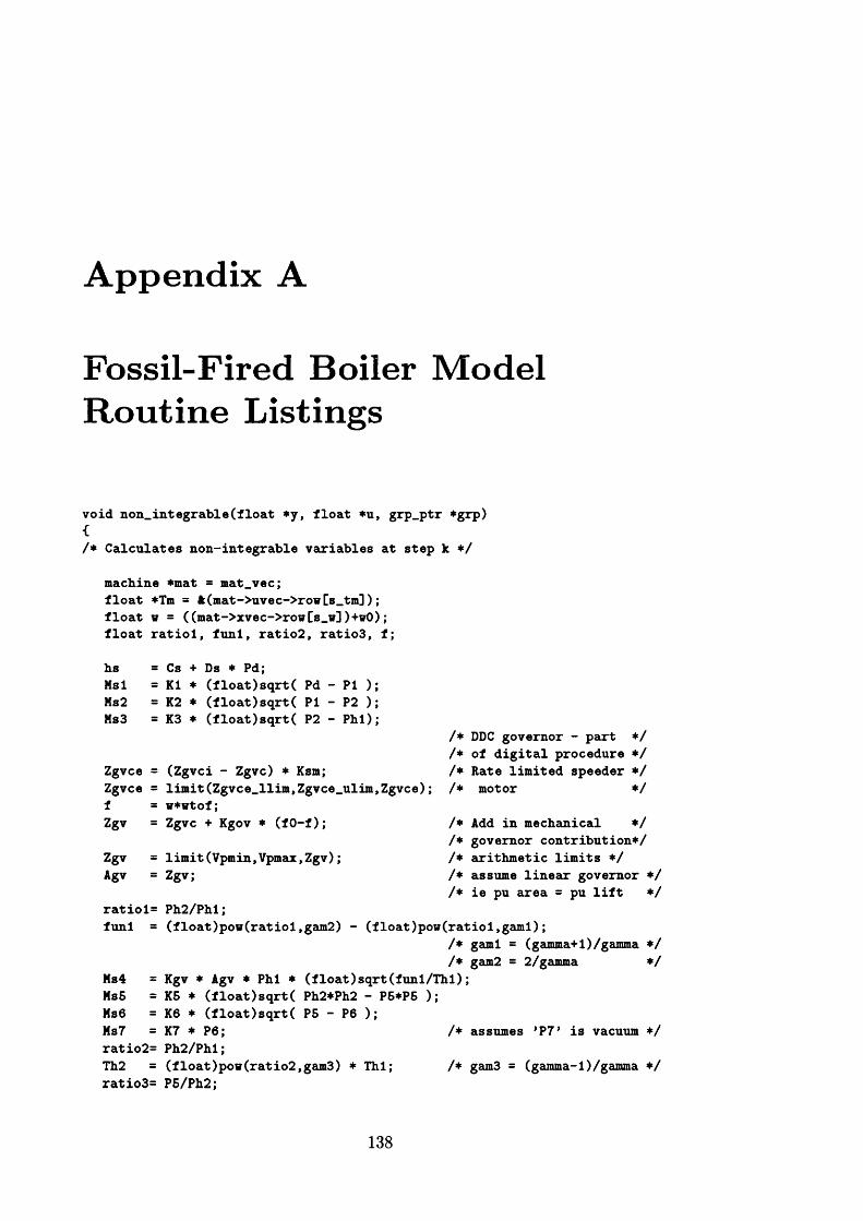
A p p en d ix A
Fossil-F ired Boiler M odel R ou tin e Listings
void non_integrable(float *y, float *u, grp_ptr *grp)
/* Calculates non-integrable variables at step k */
machine *mat = mat.vec; float *Tm = A(mat->uvec->row[s_tm]); float w = ((mat->xvec->row[s_w])+w0); float ratiol, funl, ratio2, ratio3, f;
hsNslMs2Ms3
Zgvce : Zgvce s fZgv
ZgvAgv
ratiol:funl
Ms4Ms5Ms6Ms7ratio2=Th2ratio3=
CsK1K2K3
Ds * Pd;(float)sqrt( Pd - PI ) (float)sqrt( PI - P2 ) (float)sqrt( P2 - Phi)
(Zgvci - Zgvc) * Ksm;limit(Zgvce_llim,Zgvce_ulim,Zgvce);w*wtof;Zgvc + Kgov * (fO-f);
limit(Vpmin.Vpmax,Zgv);Zgv;
/* DDC governor - part *//* of digital procedure *//* Rate limited speeder *//* motor * /
/ * Add in mecheinical *//* governor contribution*//* sorithmetic limits *//* assume linear governor */ /* ie pu area = pu lift */
Ph2/Phl;(float)pov(ratiol,gam2) - (float)pov(ratiol,garni);
/* garni = (gamma+1)/gamma */ /* gam2 = 2/gamma */
Kgv * Agv * Phi * (float)sqrt(funl/Thl);K5 * (float)sqrt( Ph2*Ph2 - P5*P5 );K6 * (float)sqrt( P5 - P6 );K7 * P6; /* assumes *P7* is vacuum */Ph2/Phl;(float)po«(ratio2,gam3) * Thl; /* gam3 = (gamma-1)/gamma */P5/Ph2;
138
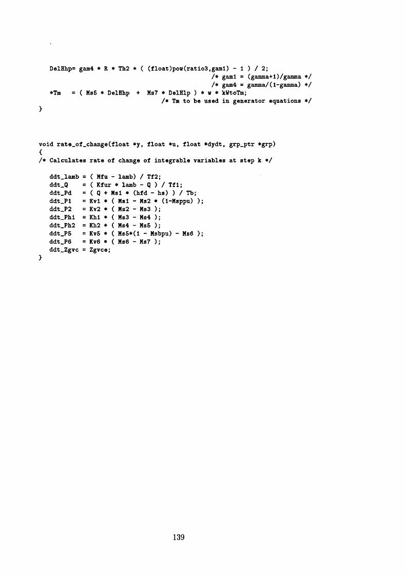
DelHhp= gam4 * R * Th2 * ( (float)pow(ratio3,garni) - 1 ) / 2;/* garni = (gamma+1)/gamma * // * gam4 = gamma/(1-gamma) */
*Tm = ( Ms5 * DelHhp + Ms7 * DelHlp ) * w * kWtoTm;/* Tm to be used in generator equations */
void rate_of.change(float *y, float *u, float *dydt, grp_ptr *grp)
Calculates rate of change of integrable variables
ddt_lamb = ( Mfu - lamb) / Tf2;ddt.Q = ( Kfur * lamb - Q ) / Tfl;ddt_Pd = ( Q + Msl * (hfd - hs) ) / Tb;ddt_Pl = Kvl * ( Msl - Ms2 * (1-Msppu) );ddt_P2 = Kv2 * ( Ms2 - Ms3 );ddt.Phl = Khl * ( Ms3 - Ms4 );ddt_Ph2 = Kh2 * ( Ms4 - Ms5 );ddt_P5 = Kv5 * ( Ms5*(l - Msbpu) - Ms6 );ddt_P6 = Kv6 * ( Ms6 - Ms7 );ddt_Zgvc = Zgvce;
139
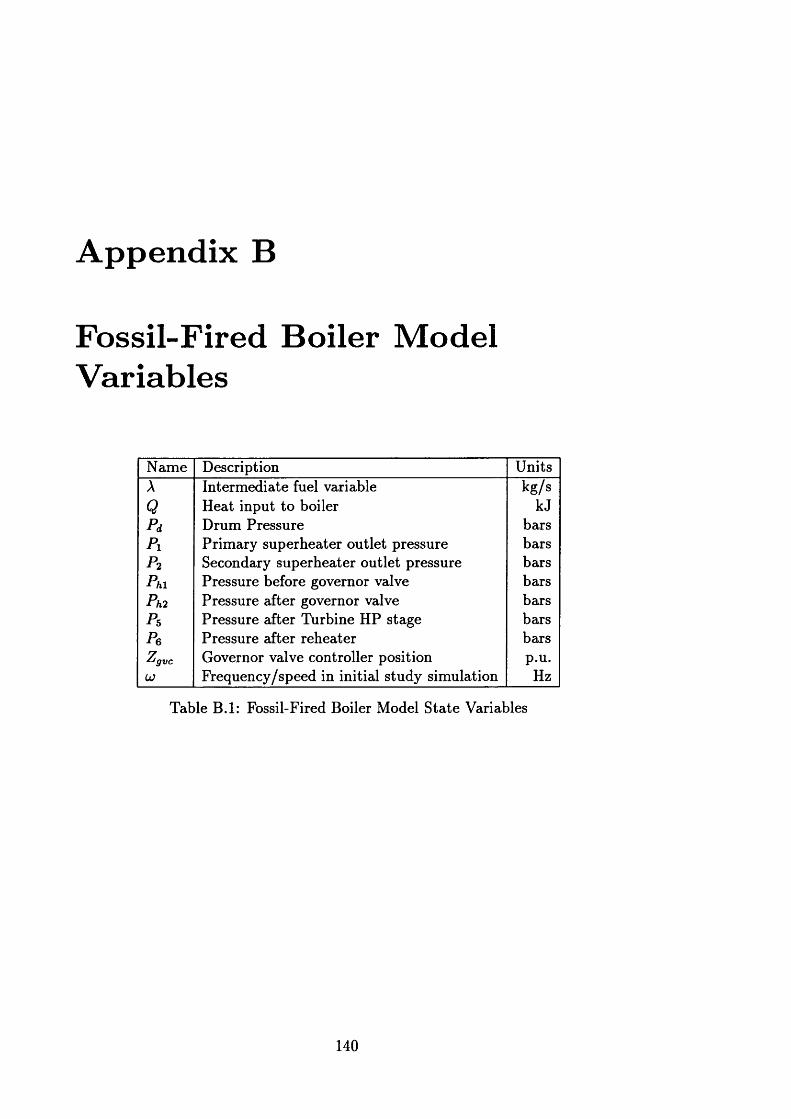
A ppendix B
Fossil-Fired Boiler M odel Variables
Name Description UnitsA Interm ediate fuel variable kg/sQ Heat input to boiler kJPd Drum Pressure barsPi Prim ary superheater outlet pressure barsP2 Secondary superheater outlet pressure barsPhi Pressure before governor valve barsPh2 Pressure after governor valve barsPs Pressure after Turbine HP stage barsPe Pressure after reheater barsZgvc Governor valve controller position p.u.(jJ Frequency/speed in initial study simulation Hz
Table B .l: Fossil-Fired Boiler Model S tate Variables
140
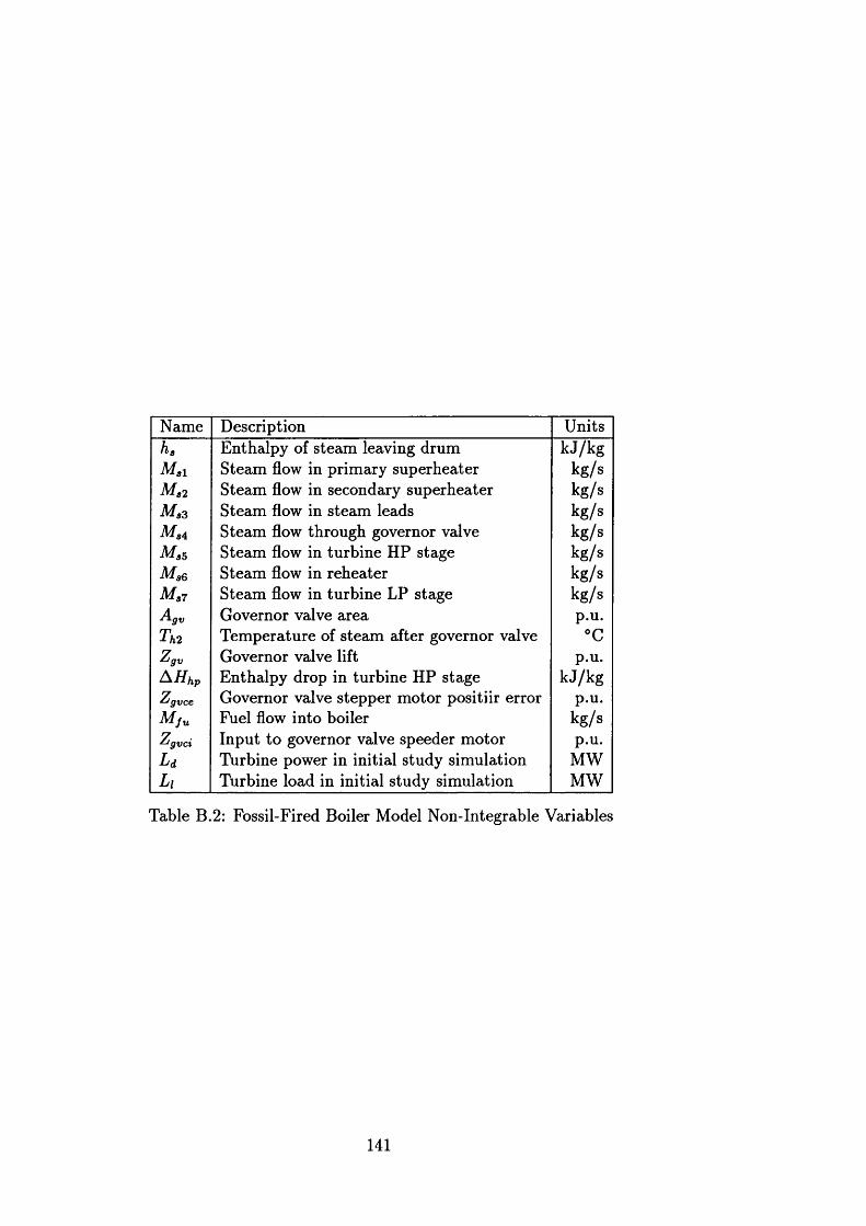
Name Description Unitsha Enthalpy of steam leaving drum kJ/kgM al Steam flow in prim ary superheater kg/sM a2 Steam flow in secondary superheater kg/sM a3 Steam flow in steam leads kg/sM a4 Steam flow through governor valve kg/sM a5 Steam flow in turbine HP stage kg/s
Steam flow in reheater kg/sM a 7 Steam flow in turbine LP stage kg/sASlgv Governor valve area p.u.Th2 Tem perature of steam after governor valve °CZgV Governor valve lift p.u.A H hp Enthalpy drop in turbine HP stage kJ/kgZgvce Governor valve stepper motor positiir error p.u.M fu Fuel flow into boiler kg/sZgvd Input to governor valve speeder motor p.u.L d Turbine power in initial study simulation MWLi Turbine load in initial study simulation MW
Table B.2: Fossil-Fired Boiler Model Non-Integrable Variables
141
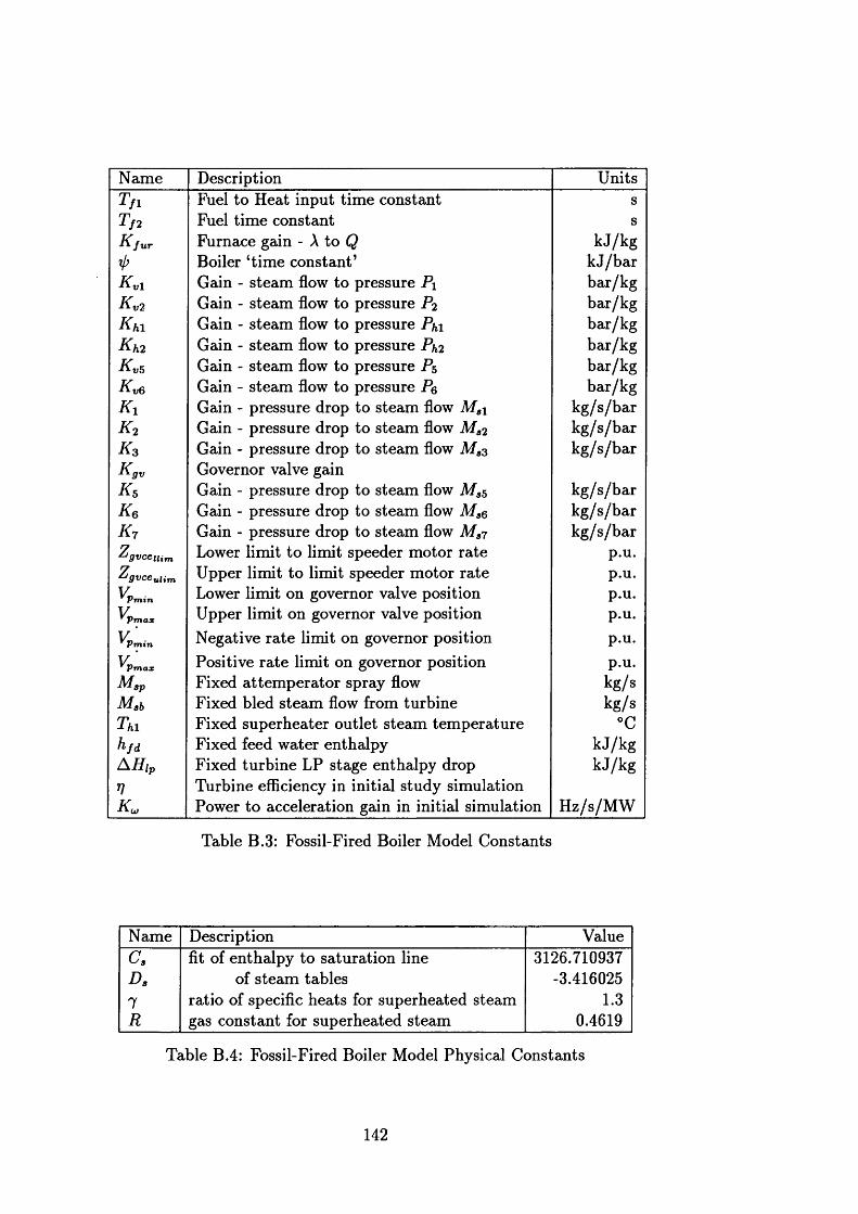
Name Description UnitsT n Fuel to Heat input tim e constant sTf2 Fuel tim e constant sK jUT Furnace gain - A to Q kJ/kg
Boiler ‘tim e constant’ k J /b a rK v i Gain - steam flow to pressure Pi bar/kgK v 2 Gain - steam flow to pressure P2 bar/kgK hl Gain - steam flow to pressure Phi bar/kgK h 2 Gain - steam flow to pressure Ph2 bar/kgK v 5 Gain - steam flow to pressure P$ bar/kgK v 6 Gain - steam flow to pressure P$ bar/kgK x Gain - pressure drop to steam flow M si kg /s /b a rk 2 Gain - pressure drop to steam flow M a2 k g /s /b a rk 3 Gain - pressure drop to steam flow M a3 k g /s /b a rKgV Governor valve gainK 5 Gain - pressure drop to steam flow M a5 kg /s /b a rK 6 Gain - pressure drop to steam flow M ae k g /s /b a rI< 7 Gain - pressure drop to steam flow M a7 kg /s /b a rZgvcetum Lower limit to limit speeder motor rate p.u.Zgvceulim Upper limit to limit speeder motor rate p.u.vPmin Lower limit on governor valve position p.u.vPmax Upper limit on governor valve position p.u.vPmin Negative ra te limit on governor position p.u.y 'Pmax Positive ra te limit on governor position p.u.M sp Fixed at tem per ator spray flow kg/sM ab Fixed bled steam flow from turbine kg/sTh i Fixed superheater outlet steam tem perature °Ch/d Fixed feed water enthalpy kJ/kgAHlp Fixed turbine LP stage enthalpy drop kJ/kgV Turbine efficiency in initial study simulation
Power to acceleration gain in initial simulation H z/s/M W
Table B.3: Fossil-Fired Boiler Model Constants
Name Description Valuec a fit of enthalpy to saturation line 3126.710937Da of steam tables -3.4160251 ratio of specific heats for superheated steam 1.3R gas constant for superheated steam 0.4619
Table B.4: Fossil-Fired Boiler Model Physical Constants
142
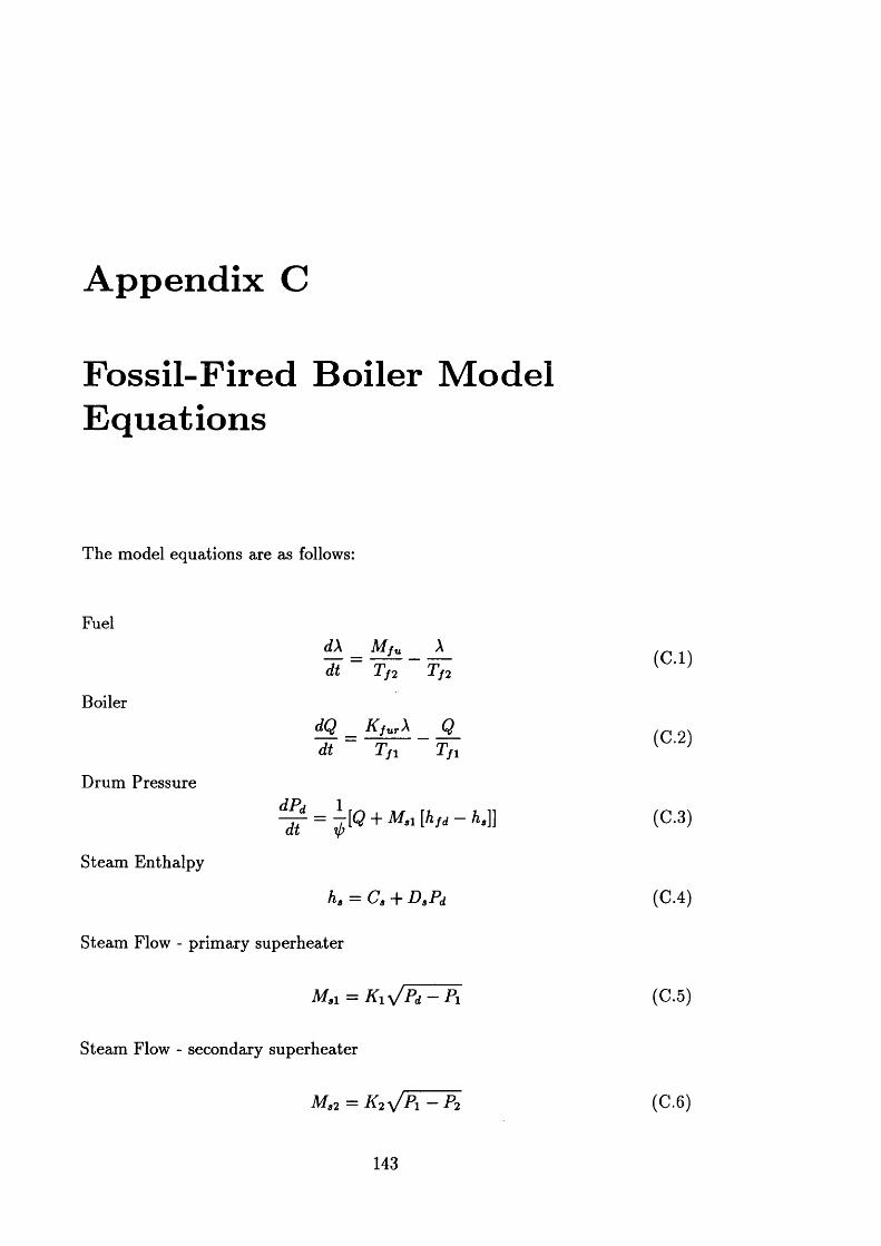
A ppendix C
Fossil-Fired Boiler M odel Equations
The model equations are as follows:
Fuel
Boiler
Drum Pressure
Steam Enthalpy
dX M fu Xdt T/2 T/2
dQ _ K furX Qdt T fi T fi
^ = ±[<J + M a [ h , t - A,]]
ha — Ca + DaPd
Steam Flow - prim ary superheater
A /,i = K1\/Pd — P\
Steam Flow - secondary superheater
m ,2 = k 2^ p 1 - p 2
(C .l)
(C.2)
(0 .3)
(C.4)
(C.5)
(C .6 )
143
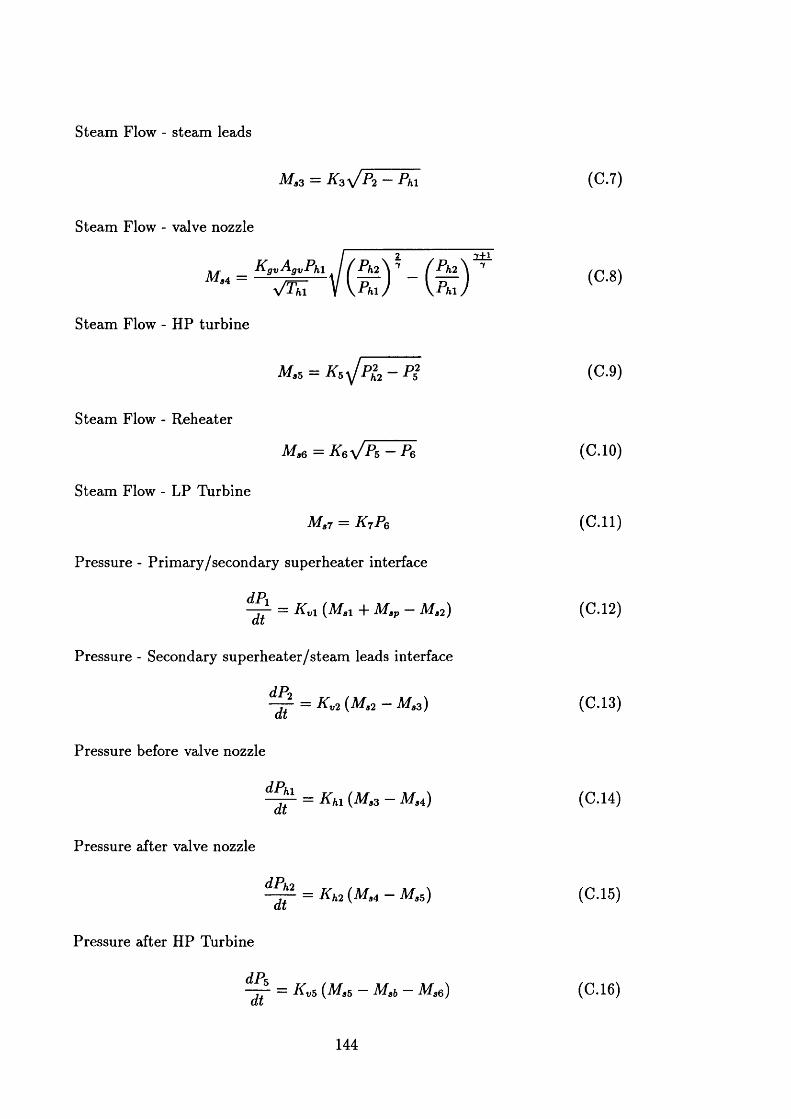
Steam Flow - steam leads
M S3 — K 3yJ P2 — P / i i
Steam Flow - valve nozzle
/ ( £ ) = _ ( £ )2±i
7
Steam Flow - HP turbine
M, 5 = K ^ P t 2 - P i
Steam Flow - Reheater
M a6 — Kq — Pq
Steam Flow - LP Turbine
M a 7 = K 7 P6
Pressure - Prim ary/secondary superheater interface
^ = K vl (A /,i + A /,p - A /,2)
Pressure - Secondary superheater/steam leads interface
dP2
dt
Pressure before valve nozzle
dPhi dt
Pressure after valve nozzle
dPh2 dt
Pressure after HP Turbine
dP5
= K v2 (M a2 - M a3)
= Kfii (M a3 - M a4)
= K h2 (Ma4 - M a5)
dt— K v 5 (M a 5 — Msb — M sq)
(C.7)
(C .8 )
(C.9)
(C.10)
(C .ll)
(C.12)
(C. 13)
(C.14)
(C.15)
(C.16)
144
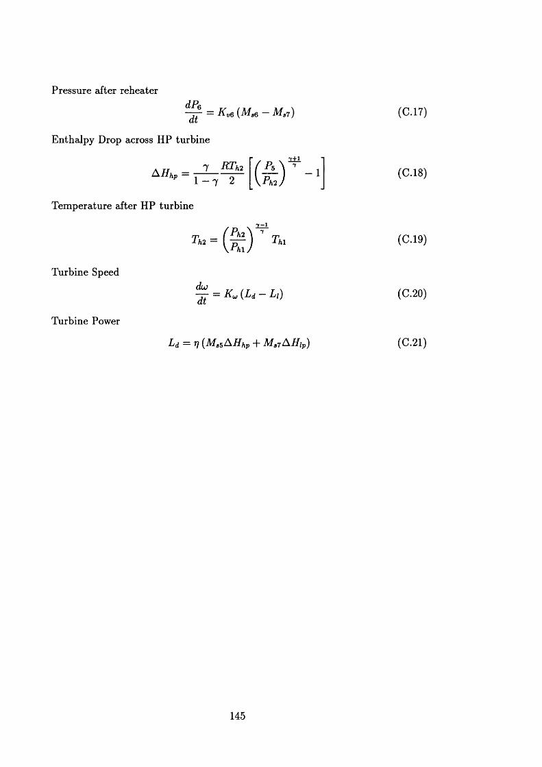
Pressure after reheaterdPedt
= Kve (M sq — M si)
Enthalpy Drop across HP turbine
7 RTh2A H hp = 1 - 7 2 ( £ f
Tem perature after HP turbine
Turbine Speed
Turbine Power
2m = 1 T u
dcudt
= K u (L d - L t )
Ld — Tj (M s5AHhp + M a7A H lp)
(C.17)
(C.18)
(C.19)
(C.20)
(C.2 1 )
145
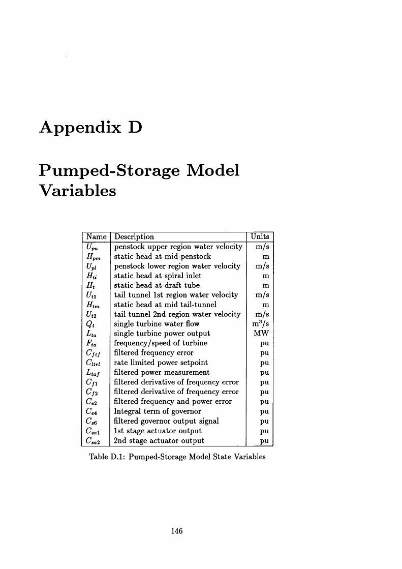
A ppendix D
P um ped-Storage M odel Variables
Name Description Unitsu pu penstock upper region water velocity m /sHpm static head at mid-penstock mu pi penstock lower region water velocity m /s
static head at spiral inlet mH t static head at draft tube mUn tail tunnel 1 st region water velocity m /sH tm static head at mid tail-tunnel mUt2 tail tunnel 2 nd region water velocity m /sQt single turbine water flow m 3/sLta single turbine power output MWFta frequency/speed of turbine puCft f filtered frequency error puUltrl ra te limited power setpoint puLtaf filtered power measurement puC j 1 filtered derivative of frequency error puCf2 filtered derivative of frequency error puCe 2 filtered frequency and power error puCe 4 Integral term of governor puc s6 filtered governor output signal puCaal 1 st stage actuator output puC30,2 2 nd stage actuator output pu
Table D .l: Pumped-Storage Model S tate Variables
146
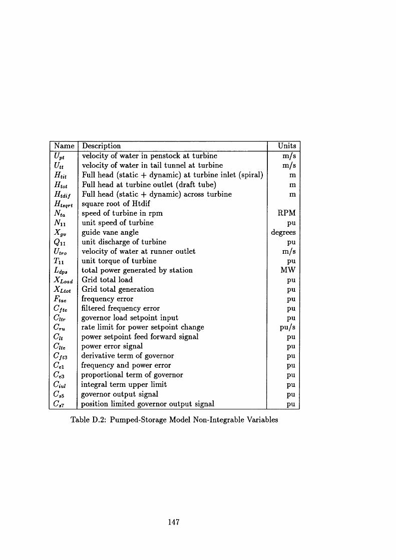
Name Description Unitsupt velocity of water in penstock at turbine m /sutt velocity of water in tail tunnel at turbine m /sH tit Full head (static + dynamic) at turbine inlet (spiral) mHtot Full head at turbine outlet (draft tube) mHtdtf Full head (static + dynamic) across turbine mHfsqrt square root of HtdifN ta speed of turbine in rpm RPMN n unit speed of turbine puXgv guide vane angle degreesQ n unit discharge of turbine puUtro velocity of water at runner outlet m /sT\\ unit torque of turbine puLdps to tal power generated by station MWXLoad Grid to tal load puXHot Grid total generation puHtoe frequency error puCfte filtered frequency error puCltT governor load setpoint input pucru rate limit for power setpoint change pu /sCu power setpoint feed forward signal puClte power error signal pucft3 derivative term of governor puCel frequency and power error puCe3 proportional term of governor puC%ul integral term upper limit pucs5 governor output signal puca7 position limited governor output signal pu
Table D.2: Pumped-Storage Model Non-Integrable Variables
147
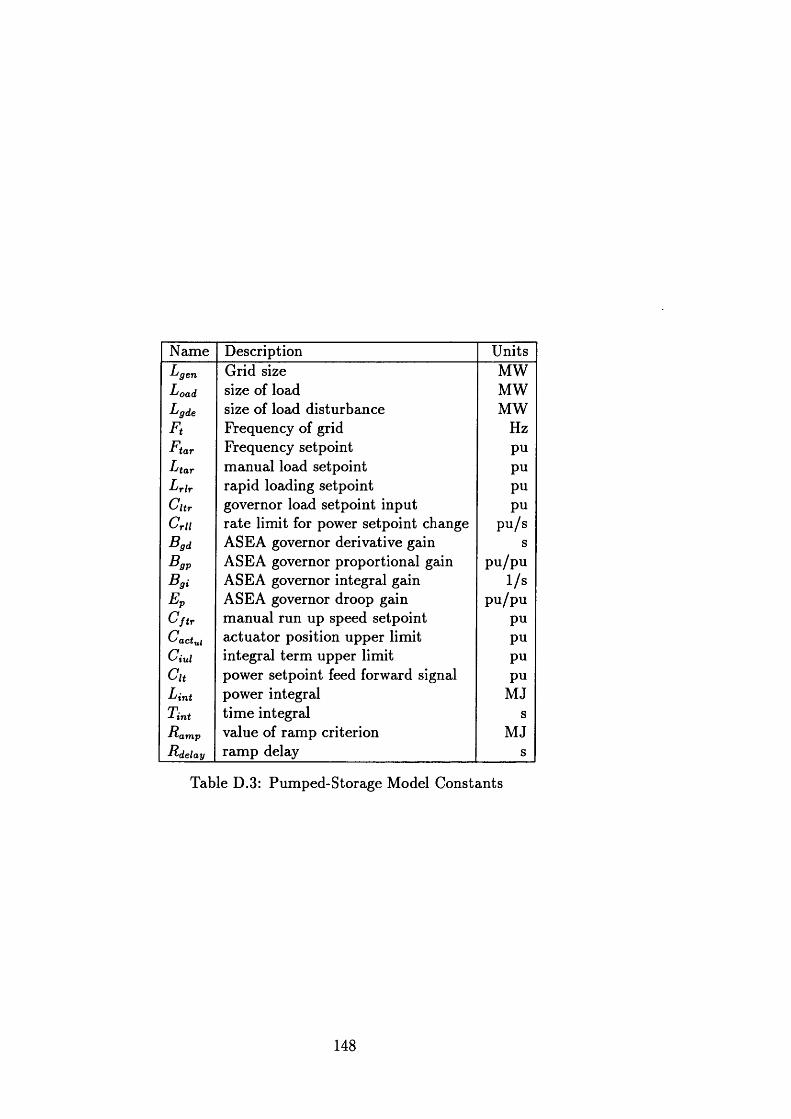
Name Description UnitsLgen Grid size MWLoad. size of load MWLgde size of load disturbance MWFt Frequency of grid HzFtar Frequency setpoint puLtar m anual load setpoint puLrlr rapid loading setpoint puCltr governor load setpoint input puCrll ra te limit for power setpoint change pu /sBgd ASEA governor derivative gain sBgp ASEA governor proportional gain pu /p uB gi ASEA governor integral gain 1/sFP ASEA governor droop gain p u /puCJir manual run up speed setpoint puCactui actuator position upper limit puCivl integral term upper limit puCu power setpoint feed forward signal puLint power integral MJTint tim e integral sRamp value of ram p criterion MJRdelay ram p delay s
Table D.3: Pumped-Storage Model Constants
148
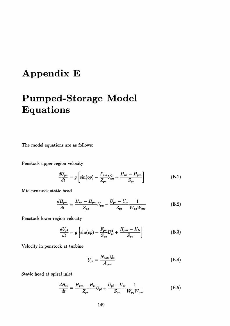
A ppendix E
P um ped-Storage M odel Equations
The model equations are as follows:
Penstock upper region velocity
dUtpudt = 9
Hlir Hr \ ± P™tt2 , " t t rsm {op) - -^—Upu + ----- ?-------'pe
Mid-penstock static head
dHrtm H ut H*dt
Penstock lower region velocity
dUpl
pm -"ur * * p m j T . U pu U p\ 1
~z pu z w wUne. r r nn r r t)'pe r r pg r r ptz;
dt = 9pw t t 2 i Hpm Hti
z Z u”' + ~ Zsin(op) - - ^ U 2pt +pe ^ p e
Velocity in penstock at turbine
Upt =Hgets Q i
lpen
Static head a t spiral inlet
dHti Hpm Hti TT . Upi Upt 1
n r = — — u * +'pe
(E.1)
(E.2)
(E.3)
(E.4)
(E.5)
149
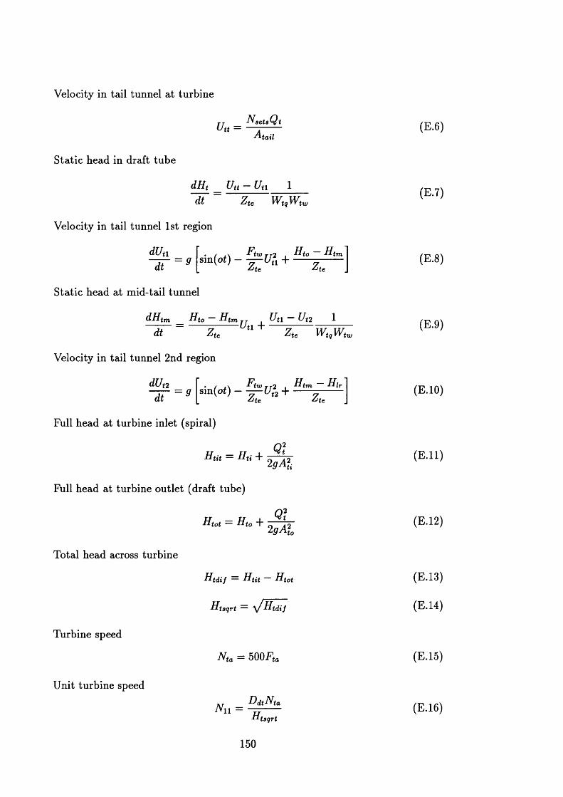
Velocity in tail tunnel at turbine
Utt =H Sets Q t
A-tail
Static head in draft tube
dHt Utt - Un 1dt Zte WtqWfw
Velocity in tail tunnel 1st region
dUi*idt = 9 M o t ) - -7T~Ua +
tw j j2 , Hto Htm
Jte He
Static head at mid-tail tunnel
dt Z te
Velocity in tail tunnel 2nd region
dUn
dHtm Ht0 — H tm TT Uti — Ut2 1—Utl + WtgW tw
dt = 9 sin (at) - +Ftxu t t2 , Htm Hlr Zte ^te
Full head at turbine inlet (spiral)
Hut = H ti +
Full head at turbine outlet (draft tube)
H tot — H t0 +
Q \2 g A l
Q 2t2 g A l
Total head across turbine
H tdif — Hfit Htot
Htsqrt — y j H tdif
Turbine speed
N ta — bOOFta
Unit turbine speedDdtNta
11 “ -------Htsqrt
150
(E.6)
(E.7)
(E.8)
(E.9)
(E.10)
(E .l l)
(E.12)
(E.13)
(E.14)
(E.15)
(E.16)
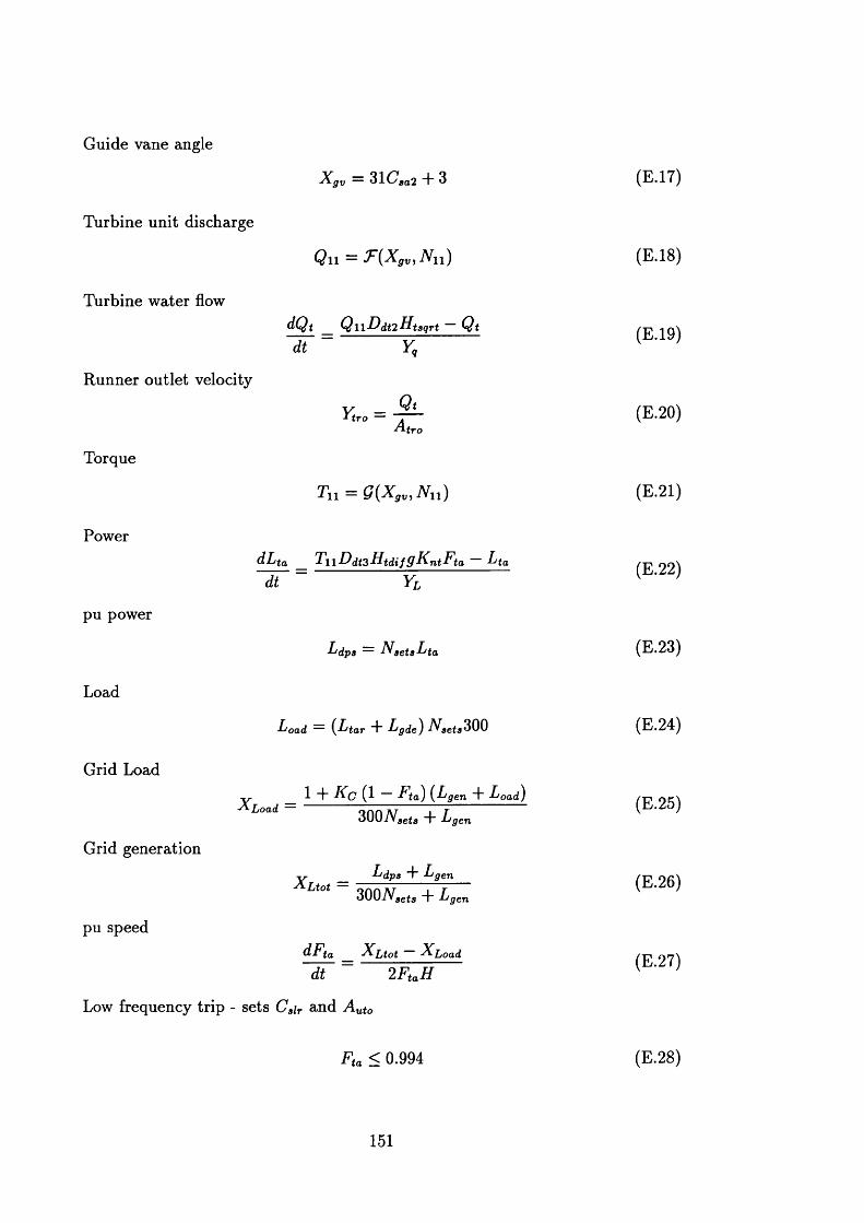
Guide vane angle
Turbine unit discharge
Turbine water flow
Runner outlet velocity
Torque
X gv = 31(7*02 + 3
O n — F ( X g v , N n )
dQt QllDdtlHtsqrt Qt~ d f ~ Y„
V —jl i.rn —U ro
T11= g { X gv,Nn )
Power
pu power
Load
Grid Load
Grid generation
pu speed
d L f a T w D d tzH td i fQ ^n tF ta Lta
~ d T ~ Yl
Ldps — X 3ets L/ta
Load — (Ltor + Lgde) N aets300
Xjjoad —1 ~f~ K C (1 F tq) (-L gen "1“ Load)
3001V„,(s + Lgen
ir Ldps “f- LgenUOt ~ 300iV«(s + Lgen
dFps sC^tot ^sLoaddt 2 Fu,H
Low frequency trip - sets C»ir and Auto
Fta < 0.994
151
(E.17)
(E.18)
(E.19)
(E.20)
(E.21)
(E.22)
(E.23)
(E.24)
(E.25)
(E.26)
(E.27)
(E.28)
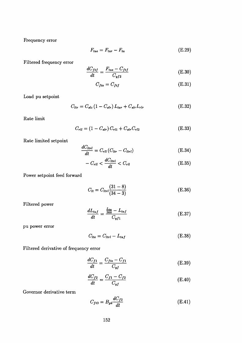
Frequency error
Ftae ~ Ffar Ffa
Filtered frequency errord C f t f _ F fae C i t l
dt C y f 2
C f t e — C f t f
Load pu setpoint
C l t r = C 9lc (1 — C3lr) d tar d" CslrLrlr
R ate limit
Crll = (1 — Csir) Crll + C 8lr C rl2
R ate limited setpointdCuri (n n \
^ o rll {^Itr — o Itrl)
- C rU < < CrU
Power setpoint feed forward
_ (31 - 8)" r ,(34 — 3)
Filtered powerd L t a f 300 ~ d / t a f
dt C y f l
pu power error
Cite = Cltrl d/taf
Filtered derivative of frequency error
dCf 1 ^ Cfte - C/1
(I/t yf
dCn Cn - Cndt C y f
Governor derivative term
r - rC/t3 ~ Bgd ^
(E.29)
(E.30)
(E.31)
(E.32)
(E.33)
(E.34)
(E.35)
(E.36)
(E.37)
(E.38)
(E.39)
(E.40)
(E.41)
152
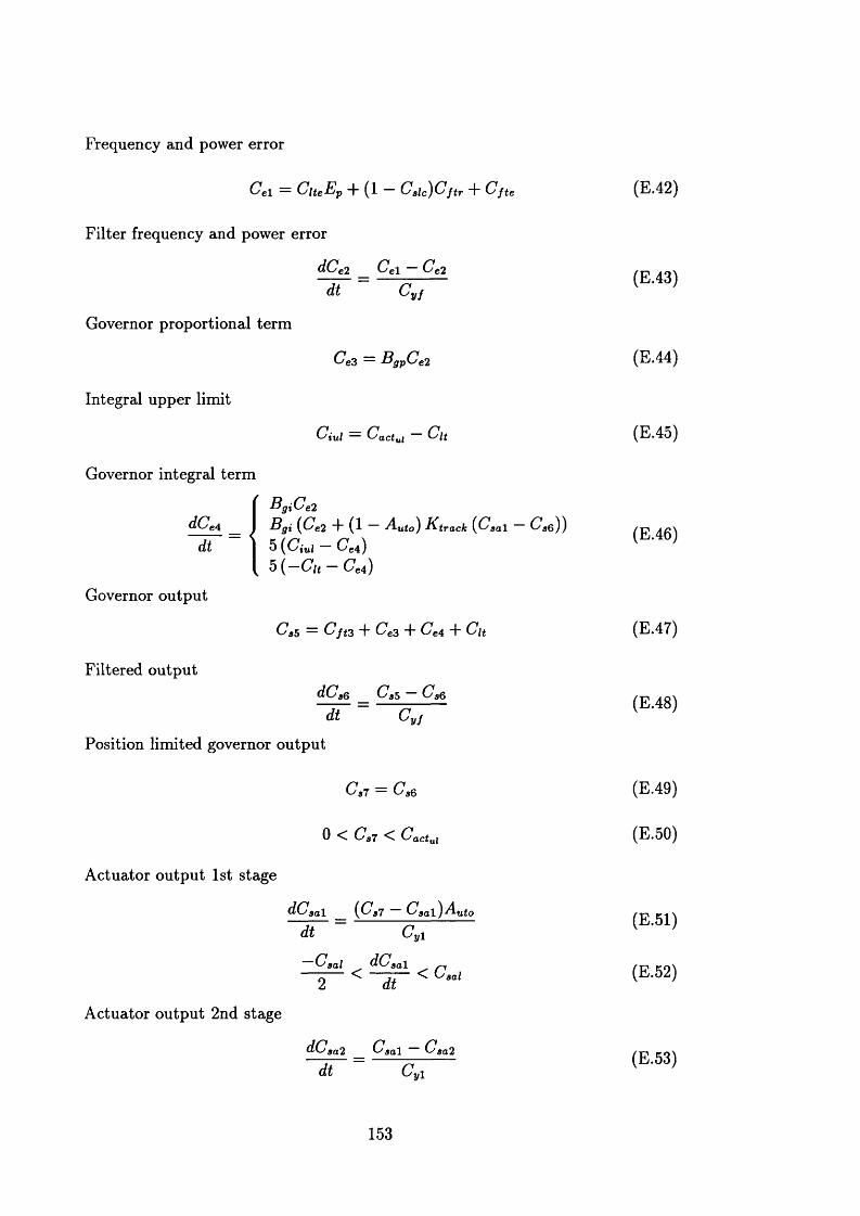
Frequency and power error
Cel — ClteEp -f (1 — C alc)Cjtr + Cfte
Filter frequency and power error
dCe 2 Cel — Ce 2dt CyJ
Governor proportional term
Integral upper limit
Ce3 — BgpCe 2
C\ui — Cactu j C\t
Governor integral term
dCte4dt
Governor output
Filtered output
f BgiCe 2(Ce2 “I" (1 — A uto) Ktrack {Csa 1 _ G ^ ))
5 (C iul ~ C e 4 ){ 5 ( - C i t - C U )
CsS = Cft3 + Ce 3 + Ce4 + Clt
dCa6 _ Cs 5 ~ C, dt 'yf
Position limited governor output
C si — CSQ
0 < Ca7 ^ Cactui
Actuator output 1st stage
dCsa 1 {Csi Caai)A utodt Cyl
Csal dCsa 1 ^~~2 ~ ~ i r c ’°l
Actuator output 2nd stage
dCSa2 CSa\ CSa2
dt C' yl
(E.42)
(E.43)
(E.44)
(E.45)
(E.46)
(E.47)
(E.48)
(E.49)
(E.50)
(E.51)
(E.52)
(E.53)
153
A ppendix F
Four Equivalent M achine Study
NETWORK proc 16 tstep .02PROCESSORS 16
* default governorGOV simple G000 reg 0.04 ta 0.3 tb 0.5 tc 10. kl 1. vpmax 1.1 vpmin \
-1.1 pvpmax 0.2 pvpmin -5. constant power
* Busbar data :-GET "study/m4/b6gen.std"GET "study/govs"GET "study/m4/m4tan"
GET "study/m4/p6"
* GROUP Specifications :-
GROUP DINORWIG bbar DIN04 set DIN001 avr A001 gov dinogov no 6 \vt 1.00346 mw 1000.0 mvar -223.652 area 1
GROUP CEGB bbar CEGB4 set CEGB01 avr A001 gov pembgovsus no 20\vt 0.996656 mw 9677.88 mvar -3.10936 area 1
GROUP NWALES bbar NWAL4 set NWAL01 avr A001 gov pembgovsus no 1 \vt 0.997527 mw 339.116 mvar -66.0287 area 1
GROUP SCOTLAND bbar SC0T4 set SC0T01 avr A001 gov pembgovsus no 4 \ vt 1.00511 mw 1810.95 mvar 18.0024 area 2
F . l M a ster F ile
* Four machine study with Dinorwig generating*
154
* Load data
* LOAD L001 pvO 100 qvO 100 LOAD L001 pfl 100 qfl 100LOADGROUP LDEES4 bbar DEES4 load L001 mw -2500 mvar 0.0LOADGROUP LPENT4 bbar PENT4 load L001 mw -200 mvar 0.0LOADGROUP LCEGB4 bbar CEGB4 load L001 mw -8200 mvar 0.0LOADGROUP LNWAL4 bbar NWAL4 load L001 mw -100 mvar 0.0LOADGROUP LSC0T4 bbar SC0T4 load L001 mw -1200 mvar 0.0
* Picture definition file for four machine study
DIAGRAM "pic.fourmach" info freq
PICTURE single overviewgroups white DINORWIG green NWALES yellow CEGB blue SCOTLAND
PICTURE single overviewbusbars white DEES4 green PENT4 yellow DIN04 blue CEGB4 magenta \
NWAL4 cyan SC0T4
DISPLAY all
END
F .2 B u sb ar and L ine D a ta
* Busbar data :-
BBAR DEES4 pg 0.00 qg 0.00 pi 2803.68 ql -521.26 \vmag 1.01819 vang -98.1135
BBAR PENT4 pg 0.00 qg 0.00 pi 247.147 ql -113.237 \vmag 1.01894 vang -93.6863
BBAR DIN04 pg 1000.0 qg -223.653 pi 0.00 ql 0.00 \vmag 1.01932 vang -93.0448
BBAR CEGB4 pg 9677.88 qg -3.10669 pi 8403.54 ql 189.12 \vmag 0.996656 vang -93.5999
BBAR NWAL4 pg 339.117 qg -66.0301 pi 113.684 ql 68.4929 \vmag 0.997527 vang -92.5236
BBAR SC0T4 pg 1810.95 qg 17.9993 pi 1243.42 ql -23.1189 \vmag 1.00511 vang -82.7423
* Line data :-
LINE name LI bbarl DEES4 bbar2 PENT4 r 0.095 x 1.264 b 52.38LINE name L2 bbarl DEES4 bbar2 PENT4 r 0.095 x 1.264 b 52.38
155
LINE bbarl PENT4 b -200LINE name LI bbarl DIN04 bbar2 PENT4 r 0.0073 X 0.121LINE name L2 bbarl DIN04 bbar2 PENT4 r 0.0094 X 0.1385LINE name L3 bbarl DEES4 bbar2 PENT4 r 0.2034 X 2.0261LINE bbarl DEES4 bbar2 CEGB4 r -0.0272 X 0.6801LINE bbarl DEES4 bbar 2 NWAL4 r 0.3008 X 8.3052LINE bbarl DEES4 bbar 2 SC0T4 r 1.0308 X 17.6785LINE bbarl PENT4 bbar2 CEGB4 r -2.4097 X 19.573LINE bbarl PENT4 bbax2 NWAL4 r 0.0348 X 1.9251LINE bbarl PENT4 bbar2 SC0T4 r -24.5471 X 1899.61LINE bbarl CEGB4 bbar2 NWAL4 r -14.9109 X 79.0945LINE bbarl CEGB4 bbar 2 SC0T4 r 0.2317 X 4.5942LINE bbarl NWAL4 bbar 2 SC0T4 r -594.561 X 7730.81
b 220 b 124.06
Tie S-N
Tie S-N
Tie S-N Tie S-N
F .3 P rim em over D a ta
GOV simple dinogovsimp \reg 0.0 ta 1. tb 100 \tc 100 kl 1. vpmax 1.1 \vpmin -1.1 pvpmax 5. pvpmin -5.
iydro dinogov \Apen 78.5398 Atail 160.368 Ati 4.15476 'Ato 11.0447 Ddt 2.03 Knt 0.0000523599 \Yq 0.01 Kgvl 31.0 Kgv2 3.0 \Atro 3.2647 Fta.ul 0.994 Crll 0.125 \Crl2 0.125 Kffl 31.0 Kff2 8.0 \Kff3 34.0 Kff4 3.0 Cyl 0.1 \Cy2 0.2 Ckll 100.0 \Cyf 0.03 Cyf 1 4.0 Cyf2 0.02 \Csal 0.166667 sinop 0.488333 Fpv 0.124616 \Zpe 600.0 sinot -0.129083 Ftw 0.0885605 \Zte 300.0 Hur 0.0 Hlr 0.0 \Wpq 5.0e-10 Wpw 9810.0 Wtq 5.0e-10 \Wtw 9810.0 Bgd 0.0 BgP 10.0 \Bgi 1.0 Ep 0.01 Cftr 0.0 \Cactul 0.903226 Ciul 0.903226 Ktrack 10.0 \Y1 0.1 pmint 0.01 Csa2inc 0.05imple pembgovsimp \reg .04 ta .3 tb .5 \tc 10 kl 1. vpmax 1.1 \vpmin 0. pvpmax 0.2 pvpmin -5.ossil pembgovsus \reg 0.04 Tfi 15. Tf2 5. \Kfur 15840.513 Tb 434078. Kvl 0.0088438 \Kv2 0.0088438 Khl 0.0576422 Kh2 0.462517 \Kv5 0.0128247 Kv6 0.0286832 Kl 120.127 \
156
K2 216.267 K3 211.294 Kgv 397.153 \K5 3.0228 K6 158.027 K7 9.362 \Zgvcemin -0.025 Zgvcemax 0.025 vpmax 1.1 \vpmin -1.1 pvpmax 5. pvpmin -5. \Ksm 0.4 Msppu 0.0303 Msbpu 0.1854 \Thl 813. hfd 1284. DelHlp 599.23 \pmint 0.1 MfuGain 1.0 ZgvGain 1.0 \Kcpp 0.6566 Kepi 0.006566 Kcli 0.00025 \sustained}ssil pembgovnonsus \reg 0.04 Tfl 15. Tf2 5. \Kfur 15840.513 Tb 434078. Kvl 0.0088438 \Kv2 0.0088438 Khl 0.0576422 Kh2 0.462517 \Kv5 0.0128247 Kv6 0.0286832 K1 120.127 \K2 216.267 K3 211.294 Kgv 397.153 \K5 3.0228 K6 158.027 K7 9.362 \Zgvcemin -0.025 Zgvcemax 0.025 vpmax 1.1 \vpmin -1.1 pvpmax 5. pvpmin -5. \Ksm 0.4 Msppu 0.0303 Msbpu 0.1854 \Thl 813. hfd 1284. DelHlp 599.23 \pmint 0.1 MfuGain 1.0 ZgvGain 1.0 \Kcpp 0.6566 Kepi 0.006566 Kcli 0.00025 \nonsustained
F .4 G en erator and A V R D a ta
* Set data :-
SET DIN001 pf .95 h 4.5 ra .117 xdd 21.6 xd 115.20 xddd 14.3 \xq 64.3 xa 10. tdd 2.6 tddd .04 tl .02 pmax .97 rt .07 xt 4.7 \ mva 330. 50.00 60.35 70.75 82.00 94.34 109.43 129.24 166.98
SET CEGB01 pf .85 h 4.46 ra .31 xdd 30.5 xd 277. xddd 22.8 \xq 263. xa 17. tdd .78 tddd .021 tl .02 pmax .88 rt 0.0 xt 0. \mva 588. 50.0 60.0 70.0 81.6 95.4 111.0 135.0 178.0
SET NWAL01 pf .85 h 4.46 ra .31 xdd 30.5 xd 277. xddd 22.8 \xq 263. xa 17. tdd .78 tddd .021 tl .02 pmax .88 rt 0.0 xt 0. \ mva 588. 50.0 60.0 70.0 81.6 95.4 111.0 135.0 178.0
SET SC0T01 pf .85 h 4.46 ra .31 xdd 30.5 xd 277. xddd 22.8 \xq 263. xa 17. tdd .78 tddd .021 tl .02 pmax .88 rt 0.0 xt 0. \mva 588. 50.0 60.0 70.0 81.6 95.4 111.0 135.0 178.0
* AVR data :-
157
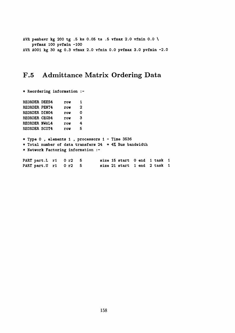
AVR pembavr kg 200 tg .5 ks 0.05 ts .5 vfmax 2.0 vfmin 0.0 \ pvfmax 100 pvfmin -100
AVR A001 kg 30 ag 0.3 vfmax 2.0 vfmin 0.0 pvfmax 3.0 pvfmin -2.0
F .5 A d m itta n ce M atrix O rdering D a ta
* Reordering information :-
REORDER DEES4 row 1REORDER PENT4 row 2REORDER DIN04 row 0REORDER CEGB4 row 3REORDER NWAL4 row 4REORDER SC0T4 row 5
* Type 0 , elements 1 , processors 1 - Time 3536* Total number of data transfers 24 * 4'/, Bus bandwidth* Network Factoring information :-
1 task 12 task 1
PART part.L rl 0 r2 5 size 15 start 0 endPART part.U rl 0 r2 5 size 21 start 1 end
158
A ppendix G
T w enty-F ive Equivalent M achine Study Files
G .l M aster F ile
NETWORK proc 16 tstep .02
* default governorGOV simple G000 reg 0.04 ta 0.3 tb 0.5 tc 10. kl 1. vpmax 1.1 \
vpmin -1.1 pvpmax 0.2 pvpmin -5. constant power
GET "study/govs"GET "study/m20/machines"* set avr and gov data
GET "study/m20/b60din"* bbar and line data
GET "study/m20/m20din"* group data
GET "study/m20/r60din"* reorder data
GET "study/m20/160din"* load data
159
G .2 P rim em over D a ta
GOV fossil Coal500 \ reg 0.04Kfur 15840.513Kv2 0.0088438Kv5 0.0128247K2 216.267K5 3.0228Zgvcemin -0.025 vpmin -1.1Ksm 0.4Thl 813.pmint 0.1Kcpp 0.6295nonsustained
GOV fossil 0il500 \ reg 0.04Kfur 15840.513Kv2 0.0088438Kv5 0.0128247K2 216.267K5 3.0228Zgvcemin -0.025 vpmin -1.1Ksm 0.4Thl 813.pmint 0.1Kcpp 0.6566nonsustained
GOV fossil Coal600 \ reg 0.04Kfur 15840.288Kv2 0.00749Kv5 0.010861K2 285.65K5 3.992Zgvcemin -0.025 vpmin -1.1Ksm 0.4Thl 813.pmint 0.1Kcpp 0.6295nonsustained
GOV fossil 0il600 \ reg 0.04Kfur 15840.288Kv2 0.00749
Tfl 40. Tf2 20. \Tb 434078. Kvl 0.0088438 \Khl 0.0576422 Kh2 0.462517 \Kv6 0.0286832 Kl 120.127 \K3 211.294 Kgv 356.04 \K6 158.027 K7 9.362 \Zgvcemax 0.025 vpmax 1.1 \pvpmax 5. pvpmin “5. \Msppu 0.0303 Msbpu 0.1854 \hfd 1284. DelHlp 599.23 \MfuGain 0.5 ZgvGain 1.0 \Kepi 0.003777 Kcli 0.00025 \
Tfl 15. Tf2 5. \Tb 434078. Kvl 0.0088438 \Khl 0.0576422 Kh2 0.462517 \Kv6 0.0286832 Kl 120.127 \K3 211.294 Kgv 356.04 \K6 158.027 K7 9.362 \Zgvcemax 0.025 vpmax 1.1 \pvpmax 5. pvpmin -5. \Msppu 0.0303 Msbpu 0.1854 \hfd 1284. DelHlp 599.23 \MfuGain 1.0 ZgvGain 1.0 \Kepi 0.006566 Kcli 0.00025 \
Tfl 40. Tf2 20.Tb 513992. Kvl 0.00749Khl 0.048816 Kh2 0.391698Kv6 0.024291 Kl 158.663K3 279.078 Kgv 470.265K6 208.72 K7 12.365Zgvcemax 0.025 vpmax 1.1pvpmax 5. pvpmin -5.Msppu 0.0303 Msbpu 0.1854hfd 1284. DelHlp 613.356MfuGain 0.422 ZgvGain 0.845Kepi 0.003777 Kcli 0.00025
Tfl 15. Tf2 5.Tb 513992. Kvl 0.00749Khl 0.048816 Kh2 0.391698
160
Kv5 0.010861 Kv6 0.024291 Kl 158.663 \K2 285.65 K3 279.078 Kgv 470.265 \K5 3.992 K6 208.72 K7 12.365 \Zgvcemin -0.025 Zgvcemax 0.025 vpmax 1.1 \vpmin -1.1 pvpmax 5. pvpmin -5. \Ksm 0.4 Msppu 0.0303 Msbpu 0.1854 \Thl 813. hfd 1284. DelHlp 613.356 \pmint 0.1 MfuGain 0.845 ZgvGain 0.845 \Kcpp 0.6566 Kepi 0.006566 Kcli 0.00025 \nonsustained
GOV hydro Hydro \Apen 78.5398 Atail 160.368 Ati 4.15476 \Ato 11.0447 Ddt 2.03 Knt 0.00005235!Yq 0.01 Kgvl 31.0 Kgv2 3.0 \Atro 3.2647 Fta_ul 0.994 Crll 0.125 \Crl2 0.125 Kffl 31.0 Kff2 8.0 \Kff3 34.0 Kff4 3.0 Cyl 0.1 \Cy2 0.2 Ckll 100.0 \Cyf 0.03 Cyf 1 4.0 Cyf2 0.02 \Csal 0.166667 sinop 0.488333 Fpw 0.124616 \Zpe 600.0 sinot -0.129083 Ftw 0.0885605 ’Zte 300.0 Hur 0.0 Hlr 0.0 \Wpq 5.0e-10 Wpw 9810.0 Wtq 5.0e-10 \Wtw 9810.0 Bgd 0.0 BgP 10.0 \Bgi 1.0 Ep 0.01 Cftr 0.0 \Cactul 0.903226 Ciul 0.903226 Ktrack 10.0 \Y1 0 pmint 0.01 Csa2inc 0.05
GOV fossil AGR \reg 0.19 Tfl 15. Tf2 5. \Kfur 15840.288 Tb 513992. Kvl 0.00749 \Kv2 0.00749 Khl 0.048816 Kh2 0.391698 \Kv5 0.010861 Kv6 0.024291 Kl 158.663 \K2 285.65 K3 279.078 Kgv 470.265 \K5 3.992 K6 208.72 K7 12.365 \Zgvcemin -0.025 Zgvcemax 0.025 vpmax 1.1 \vpmin -1.1 pvpmax 5. pvpmin -5. \Ksm 0.4 Msppu 0.0303 Msbpu 0.1854 \Thl 813. hfd 1284. DelHlp 663.18 \pmint 0.1 MfuGain 0.845 ZgvGain 0.845 \Kcpp 0.6295 Kepi 0.003777 Kcli 0.00025 \nonsustained
GOV fossil Mag147 \reg 0.19 Tfl 15. Tf 2 5. \Kfur 15841 Tb 257487. Kvl 0.014724 \Kv2 0.014724 Khl 0.095966 Kh2 0.77003 \Kv5 0.030379 Kv6 0.047754 Kl 35.133 \K2 62.953 K3 61.505 Kgv 103.36 \K5 0.87989 K6 46.0 K7 2.7252 \Zgvcemin -0.025 Zgvcemax 0.025 vpmax 1.1 \
161
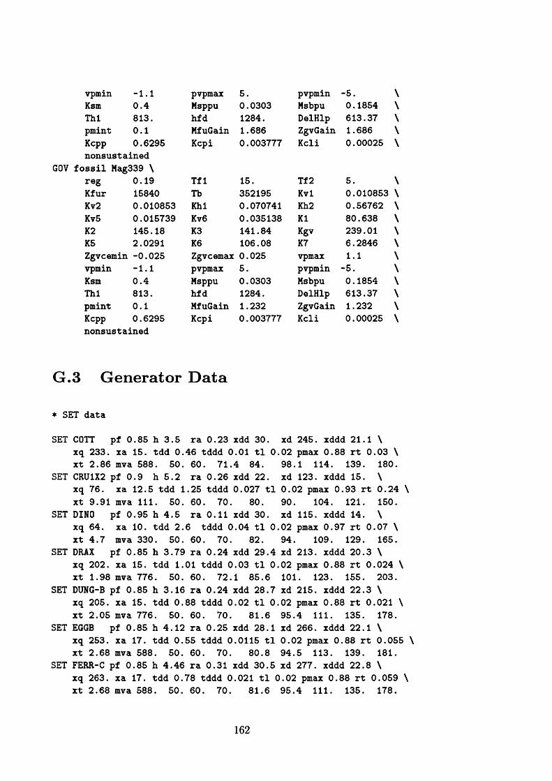
vpmin -1.1 pvpmax 5. pvpmin -5.Ksm 0.4 Msppu 0.0303 Msbpu 0.1854Thl 813. hfd 1284. DelHlp 613.37pmint 0.1 MfuGain 1.686 ZgvGain 1.686Kcpp 0.6295 nonsustained
GOV fossil Mag339 \
Kepi 0.003777 Kcli 0.00025
reg 0.19 Tfl 15. Tf 2 5.Kfur 15840 Tb 352195 Kvl 0.010853Kv2 0.010853 Khl 0.070741 Kh2 0.56762Kv5 0.015739 Kv6 0.035138 Kl 80.638K2 145.18 K3 141.84 Kgv 239.01K5 2.0291 K6 106.08 K7 6.2846Zgvcemin -0.025 Zgvcemax 0.025 vpmax 1.1vpmin -1.1 pvpmax 5. pvpmin -5.Ksm 0.4 Msppu 0.0303 Msbpu 0.1854Thl 813. hfd 1284. DelHlp 613.37pmint 0.1 MfuGain 1.232 ZgvGain 1.232Kcpp 0.6295 nonsustained
Kepi 0.003777 Kcli 0.00025
G .3 G en erator D a ta
* SET data
SET COTT pf 0.85 h 3.5 ra 0.23 xdd 30. xd 245. xddd 21.1 \xq 233. xa 15. tdd 0.46 tddd 0.01 tl 0.02 pmax 0.88 rt 0.03 \xt 2.86 mva 588. 50. 60. 71.4 84. 98.1 114. 139. 180.
SET CRU1X2 pf 0.9 h 5.2 ra 0.26 xdd 22. xd 123. xddd 15. \xq 76. xa 12.5 tdd 1.25 tddd 0.027 tl 0.02 pmax 0.93 rt 0.24 \xt 9.91 mva 111. 50. 60. 70. 80. 90. 104. 121. 150.
SET DINO pf 0.95 h 4.5 ra 0.11 xdd 30. xd 115. xddd 14. \xq 64. xa 10. tdd 2.6 tddd 0.04 tl 0.02 pmax 0.97 rt 0.07 \xt 4.7 mva 330. 50. 60. 70. 82. 94. 109. 129. 165.
SET DRAX pf 0.85 h 3.79 ra 0.24 xdd 29.4 xd 213. xddd 20.3 \xq 202. xa 15. tdd 1.01 tddd 0.03 tl 0.02 pmax 0.88 rt 0.024 \xt 1.98 mva 776. 50. 60. 72.1 85.6 101. 123. 155. 203.
SET DUNG-B pf 0.85 h 3.16 ra 0.24 xdd 28.7 xd 215. xddd 22.3 \xq 205. xa 15. tdd 0.88 tddd 0.02 tl 0.02 pmax 0.88 rt 0.021 \xt 2.05 mva 776. 50. 60. 70. 81.6 95.4 111. 135. 178.
SET EGGB pf 0.85 h 4.12 ra 0.25 xdd 28.1 xd 266. xddd 22.1 \xq 253. xa 17. tdd 0.55 tddd 0.0115 tl 0.02 pmax 0.88 rt 0.055 \xt 2.68 mva 588. 50. 60. 70. 80.8 94.5 113. 139. 181.
SET FERR-C pf 0.85 h 4.46 ra 0.31 xdd 30.5 xd 277. xddd 22.8 \xq 263. xa 17. tdd 0.78 tddd 0.021 tl 0.02 pmax 0.88 rt 0.059 \ xt 2.68 mva 588. 50. 60. 70. 81.6 95.4 111. 135. 178.
162
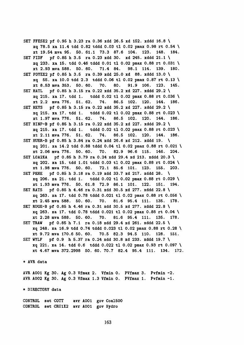
SET FFESX2 pf 0.95 h 3.23 ra 0.36 xdd 26.5 xd 152. xddd 16.8 \xq 78.5 xa 11.4 tdd 0.82 tddd 0.03 tl 0.02 pmax 0.98 rt 0.54 \ xt 19.54 mva 95. 50. 61.1 73.3 87.6 104. 123. 148. 184.
SET FIDF pf 0.85 h 3.5 ra 0.23 xdd 30. xd 245. xddd 21.1 \xq 233. xa 15. tdd 0.46 tddd 0.01 tl 0.02 pmax 0.88 rt 0.031 \ xt 2.93 mva 588. 50. 60. 71.4 84. 98.1 114. 139. 180.
SET F0YEX2 pf 0.85 h 3.5 ra 0.39 xdd 25.0 xd 88. xddd 13.0 \xq 55. xa 10.0 tdd 2.3 tddd 0.06 tl 0.02 pmax 0.87 rt 0.13 \ xt 8.53 mva 353. 50. 60. 70. 80. 91.9 106. 123. 145.
SET HATL pf 0.85 h 3.15 ra 0.22 xdd 35.2 xd 227. xddd 29.2 \xq 215. xa 17. tdd 1. tddd 0.02 tl 0.02 pmax 0.88 rt 0.036 \xt 2.2 mva 776. 51. 62. 74. 86.5 102. 120. 144. 186.
SET HEYS pf 0.85 h 3.15 ra 0.22 xdd 35.2 xd 227. xddd 29.2 \xq 215. xa 17. tdd 1. tddd 0.02 tl 0.02 pmax 0.88 rt 0.023 \xt 1.97 mva 776. 51. 62. 74. 86.5 102. 120. 144. 186.
SET HINP-B pf 0.85 h 3.15 ra 0.22 xdd 35.2 xd 227. xddd 29.2 \xq 215. xa 17. tdd 1. tddd 0.02 tl 0.02 pmax 0.88 rt 0.023 \xt 2.11 mva 776. 51. 62. 74. 86.5 102. 120. 144. 186.
SET HUER-B pf 0.85 h 3.84 ra 0.24 xdd 26.6 xd 212. xddd 19. \xq 201. xa 14.2 tdd 0.88 tddd 0.04 tl 0.02 pmax 0.88 rt 0.021 \ xt 2.06 mva 776. 50. 60. 70. 82.9 96.6 115. 146. 204.
SET L0A2XA pf 0.85 h 3.79 ra 0.24 xdd 29.4 xd 213. xddd 20.3 \ xq 202. xa 15. tdd 1.01 tddd 0.03 tl 0.02 pmax 0.88 rt 0.024 \ xt 1.98 mva 776. 50. 60. 72.1 85.6 101. 123. 155. 203.
SET PEHE pf 0.85 h 3.18 ra 0.19 xdd 33.7 xd 217. xddd 28. \xq 206. xa 21. tdd 1. tddd 0.02 tl 0.02 pmax 0.88 rt 0.029 \xt 1.93 mva 776. 50. 61.8 72.9 86.1 101. 122. 151. 194.
SET RATS pf 0.85 h 4.46 ra 0.31 xdd 30.5 xd 277. xddd 22.8 \xq 263. xa 17. tdd 0.78 tddd 0.021 tl 0.02 pmax 0.88 rt 0.056 \ xt 2.45 mva 588. 50. 60. 70. 81.6 95.4 111. 135. 178.
SET RUGE-B pf 0.85 h 4.46 ra 0.31 xdd 30.5 xd 277. xddd 22.8 \xq 263. xa 17. tdd 0.78 tddd 0.021 tl 0.02 pmax 0.88 rt 0.04 \ xt 2.28 mva 588. 50. 60. 70. 81.6 95.4 111. 135. 178.
SET TRAW pf 0.85 h 7.1 ra 0.18 xdd 29.4 xd 261. xddd 22.5 \xq 248. xa 16.9 tdd 0.74 tddd 0.023 tl 0.02 pmax 0.88 rt 0.28 \xt 9.72 mva 170.6 50. 60. 70.5 82.3 94.5 110. 128. 151.
SET WYLF pf 0.9 h 5.37 ra 0.24 xdd 30.8 xd 233. xddd 19.7 \xq 221. xa 14. tdd 0.6 tddd 0.022 tl 0.02 pmax 0.93 rt 0.097 \ xt 4.67 mva 372.2998 50. 60. 70.7 82.4 95.4 111. 134. 172
* AVR data
AVR A001 Kg 30. Ag 0.3 Vfmax 2. Vfmin 0. PVfmax 3. Pvfmin -2.AVR A002 Kg 30. Ag 0.3 Vfmax 1.3 Vfmin 0. PVfmax 1. Pvfmin -1.
* DIRECTORY data
CONTROL set COTT avr A001 gov Coal500CONTROL set CRU1X2 avr A001 gov Hydro
163
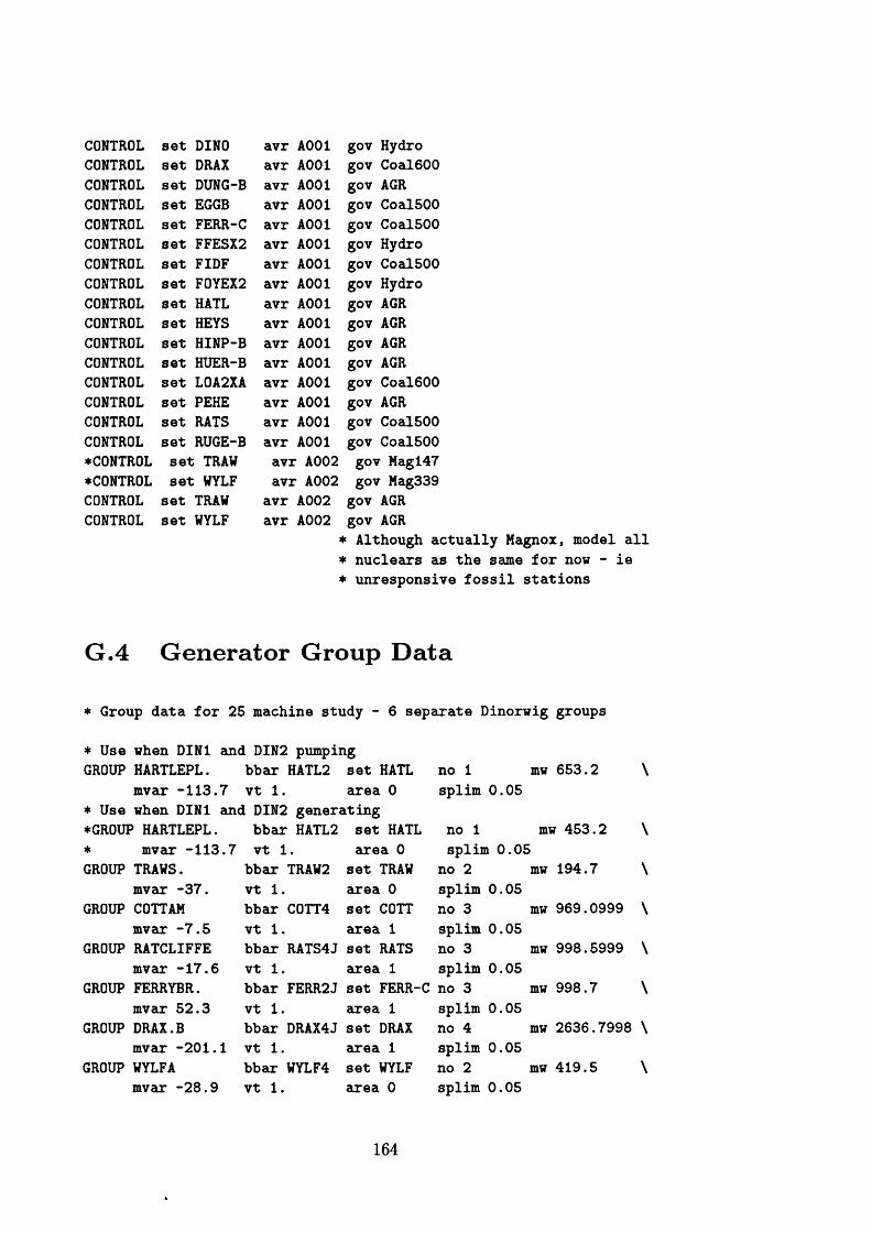
CONTROL set DINO avr A001 gov HydroCONTROL set DRAX avr A001 gov Coal600CONTROL set DUNG-B avr A001 gov AGRCONTROL set EGGB avr A001 gov Coal500CONTROL set FERR-C avr AOOl gov Coal500CONTROL set FFESX2 avr A001 gov HydroCONTROL set FIDF avr AOOl gov Coal500CONTROL set F0YEX2 avr AOOl gov HydroCONTROL set HATL avr AOOl gov AGRCONTROL set HEYS avr AOOl gov AGRCONTROL set HINP-B avr AOOl gov AGRCONTROL set HUER-B avr AOOl gov AGRCONTROL set L0A2XA avr AOOl gov Coal600CONTROL set PEHE avr AOOl gov AGRCONTROL set RATS avr AOOl gov Coal500CONTROL set RUGE-B avr AOOl gov Coal500♦CONTROL set TRAW avr A002 gov Mag147♦CONTROL set WYLF avr A002 gov Mag339CONTROL set TRAW avr A002 gov AGRCONTROL set WYLF avr A002 gov AGR
* Although actually Magnox, model all* nuclears as the same for now - ie* unresponsive fossil stations
G .4 G en erator G roup D a ta
* Group data for 25 machine study - 6 separate Dinorwig groups
* Use when DIN1 and DIN2 pumpingGROUP HARTLEPL. bbar HATL2 set HATL no 1 mw 653.2
mvar -113.7 vt 1. area 0 splim 0.05♦ Use when DIN1 and DIN2 generating♦GROUP HARTLEPL. bbar HATL2 set HATL no 1 mw 453.2♦ mvar -113.7 vt 1. area 0 splim 0.05GROUP TRAWS. bbar TRAW2 set TRAW no 2 mw 194.7
mvar -37. vt 1. area 0 splim 0.05GROUP COTTAM bbar C0TT4 set COTT no 3 mw 969.0999
mvar -7.5 vt 1. area 1 splim 0.05GROUP RATCLIFFE bbar RATS4J set RATS no 3 mw 998.5999
mvar -17.6 vt 1. area 1 splim 0.05GROUP FERRYBR. bbar FERR2J set FERR-C no 3 mw 998.7
mvar 52.3 vt 1. area 1 splim 0.05GROUP DRAX.B bbar DRAX4J set DRAX no 4 mw 2636.7998
mvar -201.1 vt 1. area 1 splim 0.05GROUP WYLFA bbar WYLF4 set WYLF no 2 mw 419.5
mvar -28.9 vt 1. area 0 splim 0.05
164
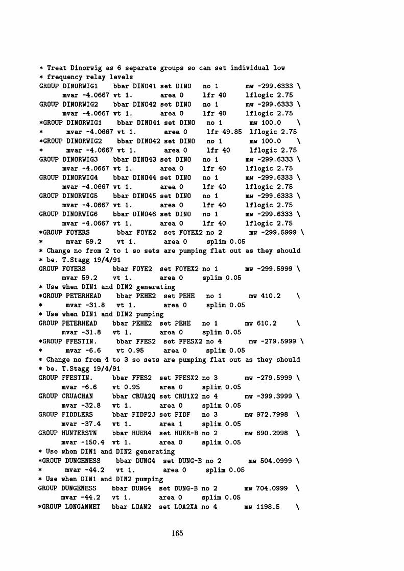
* Treat Dinorwig as 6 separate groups so can set individual low* frequency relay levelsGROUP DIN0RWIG1 bbar DIN041 set DINO no 1 mw -299.6333 \
mvar -4.0667 vt 1. area 0 lfr 40 Iflogic 2.75GROUP DIN0RWIG2 bbar DIN042 set DINO no 1 mw -299.6333 \
mvar -4.0667 vt 1. area 0 lfr 40 Iflogic 2.75♦GROUP DIN0RWIG1 bbar DIN041 set DINO no 1 mw 100.0 \♦ mvar -4.0667 vt 1. area 0 lfr 49.85 Iflogic 2.75♦GROUP DIN0RWIG2 bbar DIN042 set DINO no 1 mw 100.0 \♦ mvar -4.0667 vt 1. area 0 lfr 40 Iflogic 2.75GROUP DIN0RWIG3 bbar DIN043 set DINO no 1 mw -299.6333 \
mvar -4.0667 vt 1, area 0 lfr 40 lflogic 2.75GROUP DIN0RWIG4 bbar DIN044 set DINO no 1 mw -299,.6333 \
mvar -4.0667 vt 1. area 0 lfr 40 lflogic 2.75GROUP DIN0RWIG5 bbar DIN045 set DINO no 1 mw -299,.6333 \
mvar -4.0667 vt 1. area 0 lfr 40 lflogic 2.75GROUP DIN0RWIG6 bbar DIN046 set DINO no 1 mw -299,.6333 \
mvar -4.0667 vt 1. area 0 lfr 40 lflogic 2.75♦GROUP FOYERS bbar F0YE2 set F0YEX2 no 2 mw -299.5999 \♦ mvar 59.2 vt 1. area 0 splim 0.05♦ Change no from 2 to 1 so sets are pumping flat out as they should♦ be. T.Stagg 19/4/91GROUP FOYERS bbar F0YE2 set F0YEX2 no 1 mw -299.5999 \
mvar 59.2 vt 1. area 0 splim 0.05♦ Use when DIN1 and DIN2 generating♦GROUP PETERHEAD bbar PEHE2 set PEHE no 1 mw 410.2 \♦ mvar -31.8 vt 1. area 0 splim 0.05♦ Use when DIN1 and DIN2 pumpingGROUP PETERHEAD bbar PEHE2 set PEHE no 1 mw 610.2 \
mvar -31.8 vt 1. area 0 splim 0.05♦GROUP FFESTIN. bbar FFES2 set FFESX2 no 4 mw -279.5999 \♦ mvar -6.6 vt 0.95 area 0 splim 0.05♦ Change no from 4 to 3 so sets are pumping flat out as they should♦ be. T.Stagg 19/4/91GROUP FFESTIN. bbar FFES2 set FFESX2 no 3 mw -279.5999 \
mvar -6.6 vt 0,.95 area 0 splim 0.05GROUP CRUACHAN bbar CRUA2Q set CRU1X2 no 4 mw -399.3999 \
mvar -32.8 vt 1, area 0 splim 0.05GROUP FIDDLERS bbar FIDF2J set FIDF no 3 mw 972.7998 \
mvar -37.4 vt 1. area 1 splim 0.05GROUP HUNTERSTN bbar HUER4 set HUER-B no 2 mw 690.2998 \
mvar -150.4 vt 1. area 0 splim 0.05♦ Use when DIN1 and DIN2 generating♦GROUP DUNGENESS bbar DUNG4 set DUNG-B no 2 mw 504.0999 \♦ mvar -44.2 vt 1. area 0 splim 0.05♦ Use when DIN1 and DIN2 pumpingGROUP DUNGENESS bbar DUNG4 set DUNG-B no 2 mw 704.0999 \
mvar -44.2 vt 1. area 0 splim 0.05♦GROUP LONGANNET bbar L0AN2 set L0A2XA no 4 mw 1198.5 \
165
* mvar -235.3 vt 1. area 2 splim 0.05* Using Drax 660MW machines for Longannet, having been told by NGC* (Clive Arkell, Steve Brown, NC) that this is a station with large* sets, not little ones. - T.Stagg 19/4/91GROUP LONGANNET bbar L0AN2 set L0A2XA no 2 mw 1198.5
mvar -235.3 vt 1. area 2 splim 0.05♦Use when DIN1 and DIN2 generating♦GROUP HINKLEY bbar HINP4 set HINP-B no 2 mw 624.* mvar 18.3 vt 1. area 0 splim 0.05♦ Use when DIN1 and DIN2 pumpingGROUP HINKLEY bbar HINP4 set HINP-B no 2 mw 824.
mvar 18.3 vt 1. area 0 splim 0.05GROUP RUGELEY bbar RUGE4 set RUGE-B no 1 mw 484.3999
mvar 4.6 vt 1. area 1 splim 0.05GROUP HEYSHAM bbar HEYS4 set HEYS no 1 mw 653.2
mvar -64. vt 1. area 0 splim 0.05GROUP EGGBORO. bbar EGGB4J set EGGB no 2 mw 892.8999
mvar -30.5 vt 1. area 1 splim 0.05
166
G .5 B u sb a r and L ine D a ta
* Extra detail to treat DINORWIG as 6 separate groups
* Load Flow data
* TWENTY MACHINE , SIXTY BUSBAR REDUCTION* DINORWIG STABILISER & LINE SWITCHING STUDIES* CEGB 1984 SUMMER NIGHT MIN 22*/.(10GW) ACS DEMAND* DINORWIG IN PUMP MODE. 500MW TRANSFER FROM SSEB* ORIGINAL STUDY H.LU R4G3539,R4G3540
* Busbar data
BBAR L0VE4 vmag 0 99978 vang -36.09 Pi 423.11 qi -227.17BBAR BRF04 vmag 1 01338 vang -33.20 Pi 143.72 qi -213.40BBAR PELH4 vmag 1 00106 vang -33.38 Pi 545.08 qi -11.97BBAR DUNG4 vmag 1 00000 vang -32.83 Pi -270.30 qi 26.90BBAR SUND4 vmag 0 99433 vang -32.38 Pi 409.37 qi 39.24BBAR ECLA4 vmag 0 99550 vang -33.25 Pi 381.81 qi -32.49BBAR BRLE4 vmag 0 99900 vang -35.75 Pi 399.76 qi -71.36BBAR COWL4 vmag 0 99645 vang -34.63 Pi 75.93 qi -153.31BBAR EXET4 vmag 1 00324 vang -35.03 Pi 282.10 q1 -38.24BBAR HINP4 vmag 1 00497 vang -33.70 Pi -711.24 qi -52.25BBAR MELK4 vmag 0 99234 vang -35.13 Pi 103.17 qi 2.40BBAR WALH4 vmag 0 99662 vang -35.06 Pi -10.49 qi 84.67BBAR ABTH2J vmag 0 97360 vang -38.78 Pi 443.76 qi 92.01BBAR CILF4 vmag 0 98216 vang -37.29 Pi 170.80 qi 14.33BBAR PEMB4 vmag 0 99111 vang -37.55 Pi 129.81 qi 53.61BBAR WALP4 vmag 1 00159 vang -30.24 Pi 171.71 qi -9.74BBAR C0TT4 vmag 0 99997 vang -22.75 Pi -892.89 qi -108.09BBAR HIGM4 vmag 0 99964 vang -23.80 Pi 170.51 qi -37.86BBAR RATS4J vmag 0 99995 vang -26.70 Pi -863.85 qi -57.70BBAR WBUR4 vmag 0 99863 vang -23.18 Pi 97.06 qi -101.96BBAR CELL4 vmag 0 99785 vang -29.05 Pi 107.66 qi 35.94BBAR DRAK4 vmag 0 99717 vang -29.42 Pi 285.92 qi 67.71BBAR FECK4 vmag 0 99657 vang -32.78 Pi 180.32 qi 43.04BBAR IR0N4 vmag 0 99925 vang -32.10 Pi 229.79 qi -6.42BBAR RUGE4 vmag 0 99992 vang -29.36 Pi -459.43 qi -4.62BBAR WILL4 vmag 0 99692 vang -27.92 Pi 196.30 qi 53.39BBAR DEES4 vmag 0 99918 vang -32.61 Pi 324.13 qi -5.35BBAR LEGA4 vmag 0 99821 vang -32.85 Pi 58.71 qi 106.37BBAR PENT4 vmag 0 99969 vang -36.96 Pi 31.46 qi -9.79BBAR TRAW 2 vmag 0 99922 vang -35.44 Pi -183.44 qi 13.73BBAR TRAW4 vmag 1 00074 vang -34.98 Pi 0.0 qi 0.0
167
BBAR WYLF4 vmag 0 .99783 vang -36.60 pi -220.47 qi 105.15BBAR DIN041 vmag 0.99983 vang -37.63 pi 0.0 ql 0. 0BBAR DIN042 vmag 0.99983 vang -37.63 pi 0.0 ql 0. 0BBAR DIN043 vmag 0.99983 vang -37.63 pi 0.0 ql 0. 0BBAR DIN044 vmag 0.99983 vang -37.63 pi 0.0 ql 0. 0BBAR DIN045 vmag 0.99983 vang -37.63 pi 0.0 ql 0. 0BBAR DIN046 vmag 0.99983 vang -37.63 pi 0.0 ql 0. 0BBAR DIN04 vmag 0 99983 vang -37.63 Pi 1979.80 qi 24.43BBAR FFES2 vmag 0 99796 vang -35.67 Pi 279.57 qi 6.60BBAR FIDF2J vmag 0 99990 vang -28.34 Pi -230.33 qi -17.29BBAR DAIN4 vmag 1 00003 vang -28.94 Pi 352.28 qi -7.83BBAR HEYS4 vmag 1 00995 vang -23.07 Pi -465.39 qi -44.04BBAR PEW04 vmag 1 00726 vang -24.27 Pi 60.25 qi -64.88BBAR FERR2J vmag 1 00000 vang -16.60 Pi -528.65 ql 3.73BBAR CREB4 vmag 1 00138 vang -19.74 Pi 129.86 qi 29.10BBAR DRAX4J vmag 0 99998 vang -17.45 Pi -2464.19 ql 258.95BBAR EGGB4J vmag 0 99998 vang -18.11 Pi -859.01 qi 20.17BBAR HAWP4R vmag 1 01572 vang -16.70 Pi 26.84 qi -48.44BBAR KEAR4Q vmag 0 99315 vang -22.73 Pi 179.33 qi 8.83BBAR N0RT4Q vmag 1 01370 vang -18.08 Pi 48.90 qi -5.54BBAR 0SBA4Q vmag 1 00486 vang -17.30 Pi 28.82 qi -32.72BBAR STAL4Q vmag 0 99446 vang -22.98 Pi 118.60 qi 33.35BBAR TH0M4 vmag 0 99499 vang -20.42 Pi 353.86 qi -78.66BBAR BLYT2J vmag 1 01868 vang -16.49 Pi -90.72 qi 41.69BBAR HATL2 vmag 1 01498 vang -14.94 Pi -426.25 qi 72.87BBAR STEW2J vmag 1 02011 vang -16.55 Pi 217.27 qi -85.34BBAR HARK2 vmag 1 01196 vang -18.99 Pi 148.40 qi -108.12BBAR F0YE2 vmag 0 99999 vang -16.34 Pi 338.40 qi -52.05BBAR KINT2 vmag 1 01631 vang -9.57 Pi 138.11 qi -52.19BBAR PEHE2 vmag 1 01998 vang -7.81 Pi -550.52 qi 4.78BBAR CRUA2Q vmag 1 00501 vang -17.77 Pi 427.49 qi -9.20BBAR HUER4 vmag 1 02418 vang -10.94 Pi -460.14 qi -44.20BBAR KINC2 vmag 1 02009 vang -11.10 Pi 176.28 qi -33.84BBAR L0AN2 vmag 1 01498 vang -9.47 Pi -946.52 qi 169.58BBAR STHA2 vmag 1.02416 vang -12.87 Pi 281.20 qi -134.91
* Line data
LINE name LI bbarl L0VE4 bbar2 BRF04 r -25.8094 X 342.6487LINE name LI bbarl L0VE4 bbar2 PELH4 r -45.5669 X 354.5898LINE name LI bbarl L0VE4 bbar2 DUNG4 r 0.1574 X 2.5810LINE name LI bbarl L0VE4 bbar2 SUND4 r -186.6696 X 1319.3962LINE name LI bbarl L0VE4 bbar2 ECLA4 r -73.2008 X 619.8848LINE name LI bbarl L0VE4 bbar2 BRLE4 r 0.0670 X 0.6524LINE name LI bbarl L0VE4 bbar2 EXET4 r 0.1145 X 1.6635LINE name SI bbarl L0VE4 \
168
b -200 J0000LINE name LI bbarl BRF04 bbar2LINE name LI bbarl BRF04 bbar2LINE name LI bbarl BRF04 bbar2LINE name LI bbarl BRF04 bbar2LINE name LI bbarl BRF04 bbar2LINE name LI bbarl BRF04 bbar2LINE name L2 bbarl BRF04 bbar 2
b 45 .9393LINE name LI bbarl PELH4 bbar2LINE name LI bbarl PELH4 bbar2LINE name LI bbarl PELH4 bbar2LINE name LI bbarl PELH4 bbar2LINE name LI bbarl PELH4 bbar2LINE name LI bbarl PELH4 bbar2LINE name LI bbarl DUNG4 bbar2LINE name LI bbarl DUNG4 bbar2LINE name LI bbarl DUNG4 bbar2LINE name LI bbarl SUND4 bbar 2LINE name LI bbarl SUND4 bbar2LINE name LI bbarl SUND4 bbar2LINE name LI bbarl SUND4 bbar2LINE name LI bbarl ECLA4 bbar 2LINE name LI bbarl ECLA4 bbar2LINE name L2 bbarl ECLA4 bbar2
b 19..1900LINE name LI bbarl BRLE4 bbar 2LINE name LI bbarl BRLE4 bbar2
b 48,.1900LINE name LI bbarl C0WL4 bbar2LINE name LI bbarl C0WL4 bbar2LINE name SI bbarl C0WL4
b -200.0000LINE name LI bbarl C0WL4 bbar2
b 24.,1266LINE name L2 bbarl C0WL4 bbar2
b 93.,7054LINE name LI bbarl EXET4 bbar2LINE name LI bbarl MELK4 bbar2LINE name LI bbarl MELK4 bbar2LINE name LI bbarl MELK4 bbar2LINE name LI bbarl MELK4 bbar2LINE name SI bbarl MELK4
b -200.0000LINE name LI bbarl MELK4 bbar 2
b 50. 0014
PELH4 r -0.0994 X 14.9289DUNG4 r 0.4820 X 5.4116SUND4 r 0.5919 X 26.8656ECLA4 r 0.4491 X 18.9649BRLE4 r 0.0777 X 29.2029WALP4 r 0.3038 X 2.7027PELH4 r 0.0831 X 1.1086 \
DUNG4 r 0.2033 X 8.2666SUND4 r 0.3266 X 1.0651ECLA4 r -0.4487 X 12.4916BRLE4 r -1.1483 X 20.6784WALP4 r 0.1080 X 1.4632C0TT4 r 35.5218 X 136.5681SUND4 r 0.7113 X 24.3294ECLA4 r 0.5477 X 12.8785BRLE4 r 0.3169 X 18.6089ECLA4 r 0.2252 X 5.8471BRLE4 r 0.5620 X 10.5452C0TT4 r 0.2386 X 3.4606WBUR4 r 0.3731 X 3.2971BRLE4 r 0.2414 X 6.3296RATS4J r 0.2402 X 2.2025SUND4 r 0.0347 X 0.4631 \
C0WL4 r 0.0591 X 0.8002MELK4 r 0.1964 X 1.5546 \
MELK4 r 0.2298 X 2.2791WALH4 r 3.0580 X 57.3653
\
ECLA4 r 0.0437 X 0.5822 \
WALH4 r 0.1320 X 1.5196 \
HINP4 r 0.0729 X 0.5871WALH4 r 1.4294 X 16.2805ABTH2J r 0.6887 X 3.6260CILF4 r 0.1140 X 1.7669PEMB4 r 26.2089 X 207.9795
\
HINP4 r 0.2083 X 1.6494 \
169
LINE name L2 bbarl b 50.0014
MELK4 bbar2 HINP4 r 0.2083 X 1.6494
LINE name LI bbarl ABTH2J bbar 2 CILF4 r 0.0663 X 1.0250LINE name LI bbarl ABTH2J bbar2 PEMB4 r 0.4419 X 8.9373LINE name LI bbarl CILF4 bbar2 PEMB4 r 0.1836 X 2.7436LINE name SI bbarl
b -200.0000CILF4
LINE name L2 bbarl b 97.9100
CILF4 bbar2 PEMB4 r 0.1725 X 2.3005
LINE name LI bbarl b 109.6999
CILF4 bbar2 WALH4 r 0.1213 X 1.6282
LINE name LI bbarl b 190.4900
PEMB4 bbar2 WALH4 r 0.2637 X 3.5265
LINE name LI bbarl C0TT4 bbar2 WBUR4 r 0.1169 X 1.7705LINE name LI bbarl C0TT4 bbar2 CREB4 r 0.1852 X 1.8166LINE name LI bbarl C0TT4 bbar2 DRAX4J r 0.1682 X 2.0260LINE name LI bbarl
b 40.7232C0TT4 bbar2 RATS4J r 0.1697 X 1.3433
LINE name L2 bbarl b 5.3040
C0TT4 bbar2 WBUR4 r 0.0096 X 0.1280
LINE name LI bbarl HIGM4 bbar2 TH0M4 r 0.0857 X 3.5369LINE name LI bbarl
b 42.3955HIGM4 bbar2 RATS4J r 0.1549 X 1.2287
LINE name LI bbarl b 9.1930
HIGM4 bbar2 WBUR4 r 0.0273 X 0.2580
LINE name LI bbarl b 12.6086
RATS4J bbar2 WILL4 r 0.0525 X 0.4159
LINE name LI bbarl WBUR4 bbar2 CREB4 r 0.1399 X 1.3459LINE name LI bbarl WBUR4 bbar2 DRAX4J r 0.1277 X 1.5011LINE name SI bbarl
b -200.0000WBUR4
LINE name LI bbarl b 70.6300
WBUR4 bbar2 WALP4 r 0.1245 X 1.6594
LINE name LI bbarl b 25.9085
CELL4 bbar 2 DRAK4 r 0.1080 X 0.8546
LINE name LI bbarl b 35.8041
CELL4 bbar 2 WILL4 r 0.1492 X 1.1810
LINE name LI bbarl DRAK4 bbar2 FECK4 r 0.1250 X 1.1740LINE name LI bbarl DRAK4 bbar2 IR0N4 r 0.1833 X 4.4715LINE name LI bbarl DRAK4 bbar 2 WILL4 r 0.1036 X 8.2848LINE name LI bbarl
b 30.0000DRAK4 bbar2 RATS4J r 0.0793 X 0.6288
LINE name LI bbarl b 12.0154
DRAK4 bbar2 RUGE4 r 0.0521 X 0.3963
LINE name LI bbarl FECK4 bbar2 IR0N4 r 0.2257 X 7.7258LINE name LI bbarl FECK4 bbar2 WILL4 r 0.0889 X 10.3370
170
LINE name L2 bbarl FECK4 bbar 2b 37 .4688
LINE name LI bbarl FECK4 bbar2b 63 .1290
LINE name LI bbarl FECK4 bbar2b 40 .1285
LINE name LI bbarl IR0N4 bbar 2LINE name LI bbarl RUGE4 bbar2
b 33 .7536LINE name LI bbarl DEES4 bbar2LINE name LI bbarl DEES4 bbar2LINE name LI bbarl DEES4 bbar2LINE name LI bbarl DEES4 bbar 2LINE name LI bbarl DEES4 bbar2
b 34 .7386LINE name L2 bbarl DEES4 bbar2
b 34 .7386LINE name L2 bbarl DEES4 bbar 2
b 14 .8832LINE name LI bbarl DEES4 bbar2
b 52 .3770LINE name L2 bbarl DEES4 bbar2
b 52 .3770LINE name LI bbarl DEES4 bbar2
b 45,.2091LINE name LI bbarl LEGA4 bbar2
b 37,.1400LINE name L2 bbarl LEGA4 bbar2
b 35..1360LINE name LI bbarl LEGA4 bbar2
b 43.,6105LINE name LI bbarl PENT4 bbar2LINE name LI bbarl PENT4 bbar 2LINE name SI bbarl PENT4
b -200.0000LINE name LI bbarl PENT4 bbar 2
b 136.9016LINE name L2 bbarl PENT4 bbar2
b 23. 3455LINE name L3 bbarl PENT4 bbar2
b 23. 3455LINE name LI bbarl TRAW 2 bbar2LINE name LI bbarl TRAW2 bbar2
b 1.9296LINE name L2 bbarl TRAW2 bbar2
b 1.9296
IR0N4 r 0.1561 X 1.2359
MELK4 r 0.2572 X 2.0364
WALH4 r 0.1365 X 1.2945
WILL4 r 1.2734 X 20.6581IR0N4 r 0.1406 X 1.1134
LEGA4 r 1.9592 X 18.3865FIDF2J r 0.0274 X 1.0798HEYS4 r 1.1580 X 27.7890PEW04 r 0.0887 X 37.1891DAIN4 r 0.1508 X 1.1459
DAIN4 r 0.1508 X 1.1459
LEGA4 r 0.0661 X 0.5170
PENT4 r 0.0950 X 1.2640
PENT4 r 0.0950 X 1.2640
TRAW4 r 0.1884 X 1.4913
IR0N4 r 0.1513 X 1.1979
IR0N4 r 0.1464 X 1.1590
TRAW4 r 0.1906 X 1.4607
TRAW2 r 29.9219 X 111.9125WYLF4 r 16.8170 X 62.8052
TRAW4 r 0.0603 X 0.8215
WYLF4 r 0.0423 X 0.5634
WYLF4 r 0.0423 X 0.5634
WYLF4 r 226.2408 X 406.8196FFES2 r 0.0842 X 0.2952
FFES2 r 0.0842 X 0.2952
171
LINE name LI bbarl TRAW4 bbar2 TRAW2 r 0.0200 x 1.6000b -0.5740
LINE name L2 bbarl TRAW4 bbar2 TRAW2 r 0.0200 x 1.6000b -0.5740
* Extra lines to treat Dinorwig as 6 separate groupsLINE name
b -0LI bbarl .574
DIN041 bbar2 DIN04 r 0.02 X 1.6
LINE name b -0
LI bbarl .574
DIN042 bbar2 DIN04 r 0.02 X 1.6
LINE name b -0
LI bbarl .574
DIN043 bbar2 DIN04 r 0.02 X 1.6
LINE name b -0
LI bbarl .574
DIN044 bbar2 DIN04 r 0.02 X 1.6
LINE name b -0
LI bbarl .574
DIN045 bbar2 DIN04 r 0.02 X 1.6
LINE name b -0
LI bbarl .574
DIN046 bbar2 DIN04 r 0.02 X 1.6
LINE name LI bbarl b 124.0600
DIN04 bbar2 PENT4 r 0.0094 X 0.1385
LINE name L2 bbarl b 220.0000
DIN04 bbar2 PENT4 r 0.0073 X 0.1210
LINE name LI bbarl FIDF2J bbar2 HEYS4 r 0.2667 X 3.1693LINE name LI bbarl FIDF2J bbar2 PEW04 r 0.1896 X 4.3138LINE name LI bbarl DAIN4 bbar2 FERR2J r 0.5441 X 14.0039LINE name LI bbarl DAIN4 bbar2 KEAR4Q r 0.0011 X 3.5267LINE name LI bbarl DAIN4 bbar2 0SBA4Q r 38.9901 X 507.3882LINE name LI bbarl DAIN4 bbar2 STAL4Q r 0.0640 X 3.8385LINE name
b 31LI bbarl .2249
DAIN4 bbar 2 CELL4 r 0.1355 X 1.0300 \
LINE name LI bbarl HEYS4 bbar2 PEW04 r -0.0297 X 4.7691LINE name LI bbarl HEYS4 bbar 2 HARK2 r 0.3175 X 3.5973LINE name
b 24L2 bbarl 2281
HEYS4 bbar2 PEW04 r 0.0997 X 0.8019 \
LINE name LI bbarl PEW04 bbar2 HARK2 r 0.3709 X 4.0129LINE name
b 33LI bbarl 0008
PEW04 bbar2 DAIN4 r 0.1375 X 1.0886 \
LINE name LI bbarl FERR2J bbar2 EGGB4J r 0.0245 X 1.0165LINE name LI bbarl FERR2J bbar2 KEAR4Q r -0.3095 X 17.6632LINE name LI bbarl FERR2J bbar2 0SBA4Q r 0.3128 X 2.9619LINE name LI bbarl FERR2J bbar2 STAL4Q r 4.9395 X 68.5685LINE name LI bbarl CREB4 bbar2 DRAX4J r 0.1864 X 1.5391LINE name
b 35.L2 bbarl 5103
CREB4 bbar 2 DRAX4J r 0.0643 X 0.8570 \
LINE name b 83.
LI bbarl 0000
CREB4 bbar2 N0RT4Q r 0.1500 X 2.0000 \
172
LINE name LI bbarl DRAX4J bbar2 EGGB4J r 0.0126 b 7.1300
LINE name LI bbarl DRAX4J bbar2 0SBA4Q r 0.0970 b 26.6700
LINE name LI bbarl EGGB4J bbar2 PEW04 r 0.1874 b 89.8230
x 0 .1674 \
x 0.6266 \
x 2.2208 \
LINE name LI bbarl EGGB4J bbar 2 TH0M4 r 0.0388 X 0.4500 \b 25 .2000
LINE name LI bbarl HAWP4R bbar 2 N0RT4Q r -2.9415 X 23.2616LINE name LI bbarl HAWP4R bbar 2 0SBA4Q r 0.1675 X 2.2264LINE name LI bbarl HAWP4R bbar2 BLYT2J r 0.2675 X 7.0335LINE name LI bbarl HAWP4R bbar2 HATL2 r 0.1640 X 3.9136LINE name LI bbarl HAWP4R bbar2 STEW2J r 0.7376 X 18.5964LINE name LI bbarl KEAR4Q bbar 2 0SBA4Q r 13.0471 X 641.3445LINE name LI bbarl KEAR4Q bbar 2 STAL4Q r 0.5776 X 17.2903LINE name LI bbarl KEAR4Q bbar2 EGGB4J r 0.2140 X 1.8667 \
b 66 .7337LINE name LI bbarl N0RT4Q bbar2 BLYT2J r -0.2006 X 21.8337LINE name LI bbarl N0RT4Q bbar2 HATL 2 r 0.2260 X 4.4241LINE name LI bbarl N0RT4Q bbar2 STEW2J r 0.3236 X 5.7698LINE name LI bbarl 0SBA4Q bbar2 STAL4Q r 273.4753 X 2481.2468LINE name LI bbarl STAL4Q bbar2 TH0M4 r 0.0917 X 1.1885 \
b 127.2291LINE name SI bbarl TH0M4 \
b -200.0000LINE name LI bbarl BLYT2J bbar2 HATL2 r 0.2757 X 1.9263LINE name LI bbarl BLYT2J bbar2 STEW2J r 2.6969 X 17.1202LINE name LI bbarl BLYT2J bbar2 HARK2 r 1.0719 X 4.3264 \
b 31.0660LINE name L2 bbarl BLYT2J bbar2 HARK2 r 1.2936
b 32.8780LINE name L2 bbarl BLYT2J bbar2 STEW2J r 0.3124
b 7.1556LINE name L3 bbarl BLYT2J bbar2 STEW2J r 0.2087
b 15.4300LINE name LI bbarl HATL2 bbar2 STEW2J r 0.7552LINE name LI bbarl STEW2J bbar2 HARK2 r 13.2056LINE name LI bbarl STEW2J bbar2 HUER4 r 328.2522
tie S-NLINE name LI bbarl STEW2J bbar2 KINC2 r 0.8067
tie S-NLINE name LI bbarl STEW2J bbar2 L0AN2 r 433.6880
tie S-NLINE name LI bbarl STEW2J bbar2 STHA2 r 1.3335
tie S-NLINE name LI bbarl HARK2 bbar2 CRUA2Q r 1623.9790
x 4.4652 \
x 1.0947 \
x 1.3827 \
x 3.4342 x 90.0208 x 805.8992 \
x 7.5937 \
x 2959.3398 \
x 12.3274 \
x 3523.8098 \
173
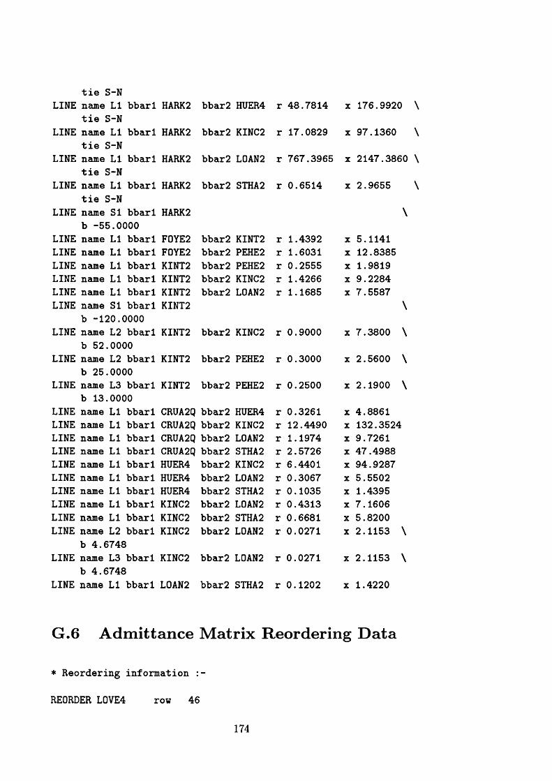
tie !S-NLINE name LI bbarl HARK2 bbar2 HUER4 r 48.7814 X 176.9920
tie :S-NLINE name
tie 1LIS-N
bbarl HARK2 bbar2 KINC2 r 17.0829 X 97.1360
LINE name LI bbarl HARK2 bbar2 L0AN2 r 767.3965 X 2147.3860tie IS-N
LINE name tie 1
LIS-N
bbarl HARK 2 bbar 2 STHA2 r 0.6514 X 2.9655
LINE name SI bbarl HARK2 \b -55.0000
LINE name LI bbarl F0YE2 bbar2 KINT2 r 1.4392 X 5.1141LINE name LI bbarl F0YE2 bbar2 PEHE2 r 1.6031 X 12.8385LINE name LI bbarl KINT2 bbar2 PEHE2 r 0.2555 X 1.9819LINE name LI bbarl KINT2 bbar2 KINC2 r 1.4266 X 9.2284LINE name LI bbarl KINT2 bbar2 L0AN2 r 1.1685 X 7.5587LINE name SI bbarl KINT2 \
b -120.0000LINE name L2 bbarl KINT2 bbar 2 KINC2 r 0.9000 X 7.3800 \
b 52 .0000LINE name L2 bbarl KINT2 bbar2 PEHE2 r 0.3000 X 2.5600 \
b 25 .0000LINE name L3 bbarl KINT2 bbar2 PEHE2 r 0.2500 X 2.1900 \
b 13 .0000LINE name LI bbarl CRUA2q bbar2 HUER4 r 0.3261 X 4.8861LINE name LI bbarl CRUA2Q bbar2 KINC2 r 12.4490 X 132.3524LINE name LI bbarl CRUA2Q bbar2 L0AN2 r 1.1974 X 9.7261LINE name LI bbarl CRUA2Q bbar2 STHA2 r 2.5726 X 47.4988LINE name LI bbarl HUER4 bbar2 KINC2 r 6.4401 X 94.9287LINE name LI bbarl HUER4 bbar2 L0AN2 r 0.3067 X 5.5502LINE name LI bbarl HUER4 bbar2 STHA2 r 0.1035 X 1.4395LINE name LI bbarl KINC2 bbar2 L0AN2 r 0.4313 X 7.1606LINE name LI bbarl KINC2 bbar2 STHA2 r 0.6681 X 5.8200LINE name L2 bbarl KINC2 bbar2 L0AN2 r 0.0271 X 2.1153 \
b 4.6748LINE name L3 bbarl KINC2 bbar2 L0AN2 r 0.0271 X 2.1153 \
b 4.6748LINE name LI bbarl L0AN2 bbar2 STHA2 r 0.1202 X 1.4220
G .6 A d m itta n ce M atrix R eord erin g D a ta
* Reordering information :-
REORDER L0VE4 row 46
174
REORDER BRF04 rowREORDER PELH4 rowREORDER DUNG4 rowREORDER SUND4 rowREORDER ECLA4 rowREORDER BRLE4 rowREORDER C0WL4 rowREORDER EXET4 rowREORDER HINP4 rowREORDER MELK4 rowREORDER WALH4 rowREORDER ABTH2J rowREORDER CILF4 rowREORDER PEMB4 rowREORDER WALP4 rowREORDER C0TT4 rowREORDER HIGM4 rowREORDER RATS4J rowREORDER WBUR4 rowREORDER CELL4 rowREORDER DRAK4 rowREORDER FECK4 rowREORDER IR0N4 rowREORDER RUGE4 rowREORDER WILL4 rowREORDER DEES4 rowREORDER LEGA4 rowREORDER PENT4 rowREORDER TRAW2 rowREORDER TRAW4 rowREORDER WYLF4 rowREORDER DIN04 rowREORDER FFES2 rowREORDER FIDF2J rowREORDER DAIN4 rowREORDER HEYS4 rowREORDER PEW04 rowREORDER FERR2J rowREORDER CREB4 rowREORDER DRAX4J rowREORDER EGGB4J rowREORDER HAWP4R rowREORDER KEAR4Q rowREORDER N0RT4Q rowREORDER 0SBA4Q rowREORDER STAL4Q row
48494550514722
23
23161314151752185354193155244
32339768501
20562125342636572935445837
175
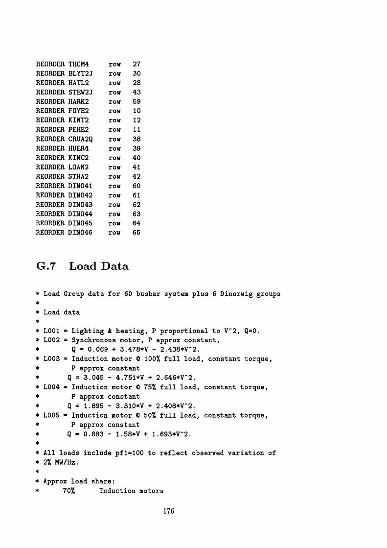
REORDER TH0M4 row 27REORDER BLYT2J row 30REORDER HATL 2 row 28REORDER STEW2J row 43REORDER HARK2 row 59REORDER F0YE2 row 10REORDER KINT2 row 12REORDER PEHE2 row 11REORDER CRUA2q row 38REORDER HUER4 row 39REORDER KINC2 row 40REORDER L0AN2 row 41REORDER STHA2 row 42REORDER DIN041 row 60REORDER DIN042 row 61REORDER DIN043 row 62REORDER DIN044 row 63REORDER DIN045 row 64REORDER DIN046 row 65
G .7 L oad D a ta
* Load Group data for 60 busbar system plus 6 Dinorwig groups*
* Load data** L001 - Lighting & heating, P proportional to V~2, Q=0.* L002 = Synchronous motor, P approx constant,* Q = 0.069 + 3.478*V - 2.438*V~2.* L003 = Induction motor <0 100*/, full load, constant torque,* P approx constant* Q = 3.045 - 4.751*V + 2.646*V~2.* L004 - Induction motor <D 75*/ full load, constant torque,* P approx constant* Q = 1.895 - 3.310*V + 2.408*V~2.* L005 - Induction motor 0 50*/ full load, constant torque,* P approx constant* Q * 0.883 - 1.58*V + 1.693*V~2.*
* All loads include pfl-100 to reflect observed variation of* 2*/, MW/Hz.*
* Approx load share:* 70/ Induction motors
176
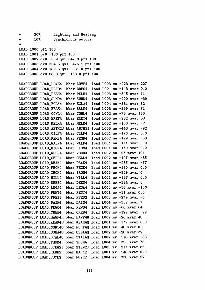
* 20% Lighting and Heating* 10% Synchronous motors*
LOAD L000 pfl 100LOAD L001 pvO -100 pfl 100LOAD L002 qvO -6.9 qvl 347.8 pfl 100LOAD L003 qvO 304.5 qvl -475.1 pfl 100LOAD L004 qvO 189.5 qvl -331.0 pfl 100LOAD L005 qvO 88.3 qvl -158.0 pfl 100
LOADGROUP L0AD.L0VE4 bbar L0VE4 load L003 mw -423 mvar 227LOADGROUP L0AD.BRF04 bbar BRF04 load L001 mw -143 mvar 0.0LOADGROUP L0AD.PELH4 bbar PELH4 load L003 mw -545 mvar 11LOADGROUP L0AD.SUND4 bbar SUND4 load L003 mw -490 mvar -39LOADGROUP L0AD.ECLA4 bbar ECLA4 load L004 mw -381 mvar 32LOADGROUP L0AD.BRLE4 bbar BRLE4 load L003 mw -399 mvar 71LOADGROUP L0AD.C0WL4 bbar C0WL4 load L002 mw -75 mvar 153LOADGROUP L0AD_EXET4 bbar EXET4 load L005 mw -282 mvar 38LOADGROUP L0AD.MELK4 bbar MELK4 load L002 mw -103 mvar -2LOADGROUP L0AD_ABTH2J bbar ABTH2J load L003 mw -443 mvar -92LOADGROUP L0AD_CILF4 bbar CILF4 load L001 mw -170 mvar 0.0LOADGROUP L0AD.PEMB4 bbar PEMB4 load L002 mw -129 mvar -53LOADGROUP L0AD.WALP4 bbar WALP4 load L001 mw -171 mvar 0.0LOADGROUP L0AD.HIGM4 bbar HIGM4 load L001 mw -170 mvar 0.0LOADGROUP L0AD.WBUR4 bbar WBUR4 load L002 mw -97 mvar 101LOADGROUP L0AD_CELL4 bbar CELL4 load L002 mw -107 mvar -35LOADGROUP L0AD.DRAK4 bbar DRAK4 load L004 mw -285 mvar -67LOADGROUP L0AD.FECK4 bbar FECK4 load L001 mw -180 mvar 0.0LOADGROUP L0AD.IR0N4 bbar IR0N4 load L005 mw -229 mvar 6LOADGROUP L0ADJJILL4 bbar WILL4 load L001 mw -196 mvar 0.0LOADGROUP L0AD.DEES4 bbar DEES4 load L004 mw -324 mvar 5LOADGROUP L0AD_LEGA4 bbar LEGA4 load L005 mw -58 mvar -■106LOADGROUP L0AD_PENT4 bbar PENT4 load L001 mw -31 mvar 0.0LOADGROUP L0AD.FFES2 bbar FFES2 load L005 mw -279 mvar -6LOADGROUP L0AD_DAIN4 bbar DAIN4 load L004 mw -352 mvar 7LOADGROUP L0AD.PEW04 bbar PEW04 load L002 mw -60 mvar 64LOADGROUP L0AD.CREB4 bbar CREB4 load L002 mw -129 mvar -29LOADGROUP L0AD.HAWP4R bbar HAWP4R load L002 mw -26 mvar 48LOADGROUP L0AD.KEAR4Q bbar KEAR4Q load L001 mw -179 mvar 0.0LOADGROUP L0AD.N0RT4Q bbar N0RT4Q load L001 mw -48 mvar C).0LOADGROUP L0AD_0SBA4Q bbar 0SBA4Q load L002 mw -28 mvar 32LOADGROUP L0AD_STAL4Q bbar STAL4Q load L002 mw -118 mvar -33LOADGROUP L0ADJTH0M4 bbar TH0M4 load L004 mw -353 mvar 78LOADGROUP L0AD.STEW2J bbar STEW2J load L005 mw -217 mvar 85LOADGROUP L0AD_HARK2 bbar HARK2 load L001 mw -148 mvar 0.0LOADGROUP L0AD.F0YE2 bbar F0YE2 load L004 mw -338 mvar 52
177
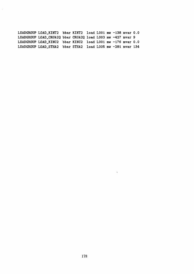
LOADGROUPLOADGROUPLOADGROUPLOADGROUP
L0AD_KINT2 bbar L0AD.CRUA2Q bbar L0AD.KINC2 bbar L0AD.STHA2 bbar
KINT2 load L001 CRUA2Q load L003 KINC2 load L001 STHA2 load L005
mw -138 mvar 0.0 mw -427 mvar 9 mw -176 mvar 0.0 mw -281 mvar 134
178
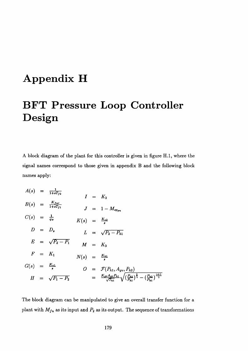
A ppend ix H
B F T Pressure Loop Controller D esign
A block diagram of the plant for this controller is given in figure H .l, where the
signal names correspond to those given in appendix B and the following block
names apply:
^ ( 5) — i+)tj2
B (s ) = irfr7T
— rl>3 T/ ( t, \ _ K x Z
I = Ko
J = 1 - M 3Ppu
D = D a
E = VPd ~ Pi
F = K i
G(s) = ^
I<(s) =
L = V P 2 - Phi
M = K 3
N (s ) = ^
0 = ^{PhllAgy^PhT)
h = - ( £ )2±i7
The block diagram can be m anipulated to give an overall transfer function for a
plant with M j u as its input and P2 as its output. The sequence of transformations
179
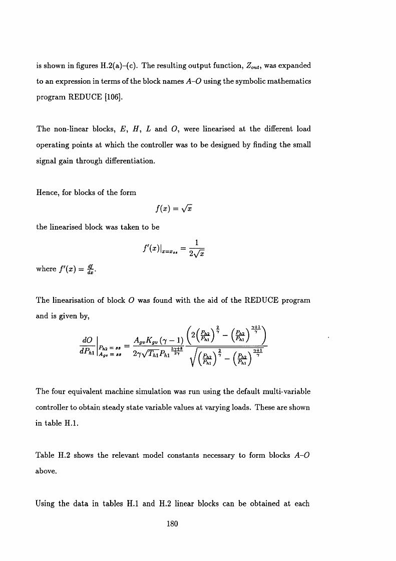
is shown in figures H .2(a)-(c). The resulting output function, Zout, was expanded
to an expression in term s of the block names A - 0 using the symbolic m athem atics
program REDUCE [106].
The non-linear blocks, E y H , L and O, were linearised at the different load
operating points at which the controller was to be designed by finding the small
signal gain through differentiation.
Hence, for blocks of the form
f ( x ) = y/x
the linearised block was taken to be
where f ' ( x ) = £•
The linearisation of block O was found with the aid of the REDUCE program
and is given by,
dOdPhi
AgxiK gv (7 — 1) V V M V Wp h2 = S3 ^ n 5 7 + 8 l~ — ----------- ;---------—•*fc2 = SS ^ „ 5*y+8 I----------------- 2---------------------------Agv = ss 2 /y y /T h iP h i ^ ^ p h2^ 1
The four equivalent machine simulation was run using the default multi-variable
controller to obtain steady state variable values at varying loads. These are shown
in table H .l.
Table H.2 shows the relevant model constants necessary to form blocks A - 0
above.
Using the data in tables H .l and H.2 linear blocks can be obtained at each
180
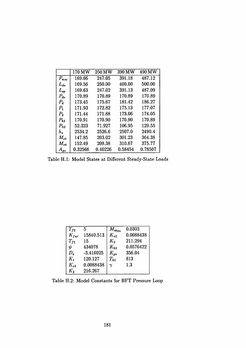
170 MW 250 MW 390 MW 490 MWp1 mw 169.66 247.05 391.18 487.12Ldv 169.56 250.00 400.00 500.00Lgp 169.63 247.02 391.13 487.09Pdv 170.89 170.89 170.89 170.89Pd 173.45 175.67 181.42 186.27P i 171.93 172.82 175.13 177.07P 2 171.44 171.88 173.06 174.05Phi 170.91 170.90 170.90 170.89Ph2 52.323 71.927 106.95 129.55ha 2534.2 2526.6 2507.0 2490.4M sl 147.85 203.02 301.23 364.38m s4 152.49 209.38 310.67 375.77AgV 0.32566 0.40226 0.58454 0.78507
Table H .l: Model States at Different Steady-State Loads
T f 2 5 M aPpu 0.0303K f u r 15840.513 K v 2 0.0088438T f i 15 k 3 211.294
434078 K h 1 0.0576422D a -3.416025 Kgv 356.04K x 120.127 Th 1 813K v 1 0.0088438 7 1.3k 2 216.267
Table H.2: Model Constants for B FT Pressure Loop
181
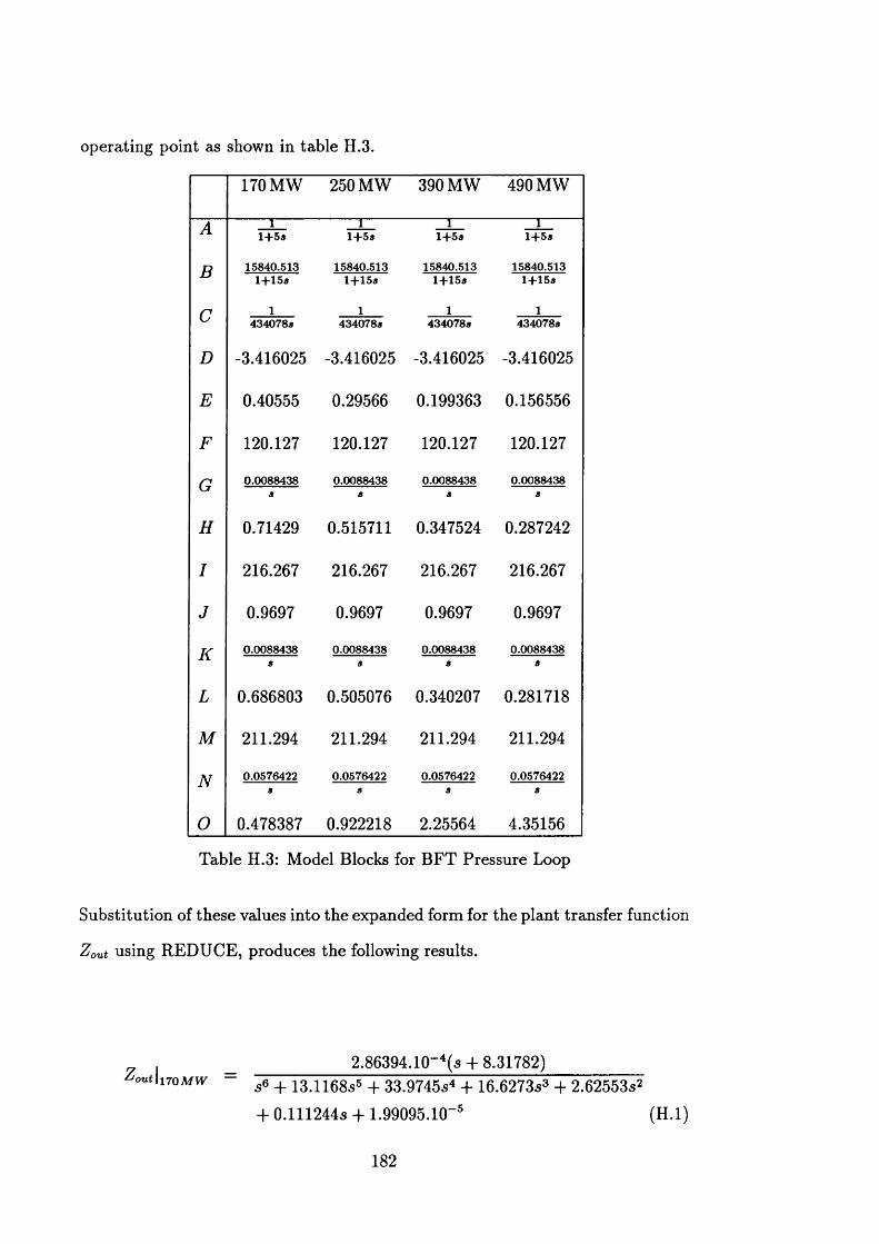
operating point as shown in table H.3.
170 MW 250 MW 390 MW 490 MW
A il + 5 a
il + 5 a
ll + 5 a
ll + 5 a
B 1 5 8 4 0 .5 1 3 1 5 8 4 0 .5 1 3 1 5 8 4 0 .5 1 3 1 5 8 4 0 .5 1 31 + 1 5 « l + 1 5 a l+ 1 5 a l+ 1 5 a
C 1 1 1 14 3 4 0 7 8 a 4 3 4 0 7 8 a 4 3 4 0 7 8 a 4 3 4 0 7 8 a
D -3.416025 -3.416025 -3.416025 -3.416025
E 0.40555 0.29566 0.199363 0.156556
F 120.127 120.127 120.127 120.127
G 0 .0 0 8 8 4 3 83
0 .0 0 8 8 4 3 83
0 .0 0 8 8 4 3 83
0 .0 0 8 8 4 3 8a
H 0.71429 0.515711 0.347524 0.287242
I 216.267 216.267 216.267 216.267
J 0.9697 0.9697 0.9697 0.9697
I< 0 .0 0 8 8 4 3 8 0 .0 0 8 8 4 3 8 0 .0 0 8 8 4 3 8 0 .0 0 8 8 4 3 8a a a a
L 0.686803 0.505076 0.340207 0.281718
M 211.294 211.294 211.294 211.294
N 0 .0 5 7 6 4 2 2 0 .0 5 7 6 4 2 2 0 .0 5 7 6 4 2 2 0 .0 5 7 6 4 2 2a a a a
0 0.478387 0.922218 2.25564 4.35156
Table H.3: Model Blocks for BFT Pressure Loop
Substitution of these values into the expanded form for the plant transfer function
Z out using REDUCE, produces the following results.
2.86394.10_4(s + 8.31782)™t\noMW - + J3.n68.s5 + 33.9745s4 + 16,6273s3 + 2.62553s2
+ 0.111244s + 1.99095.10-5 (H .l)
182
w ith open loop poles at s = —0.000179733, —0.0666674, —0.200016,-0.312197, -2.70797, -9.82988
and open loop zero at s = —8.31782
L50747.10"7(s + 6.20472)w i 250 w + 9.77539^5 + ig.0512s4 + 7.8608s3 + 1.117s2
+ 0.0465932s + 1.07362. MT* (H.2)
w ith open loop poles at s = —0.00244512, —0.0666665, —0.200015,-0.229506, -1.96174, -7.31507
and open loop zero at s = —6.20472
_ , _ 6.8498.10-5 (s -f 4.27355)A
°ui l390Mlv s 6 + 6.76681s5 + 9.44955s4 + 3.24117s3 + 0.401339s2
+ 0.016056s + 6.92132.10"5 (H.3)
w ith open loop poles at s = —0.00488374, —0.0666614, —0.159628,-0.199997, -1.33066, -5 .005
and open loop zero at s = —4.27355
, _ 4.44596.10~6(s + 3.68201)A °«<l4s>o m w se + 5.77869s5 + 6.96360s4 + 2.20837s3 + 0.257563s2
+ 0.0102876s + 6.54172.1 0 '5 (H.4)
with open loop poles at s = —0.00777324, —0.0666852, —0.133739,-0.199995, -1.10689, -4.26362
and open loop zero a t s = —3.68201
It can be seen from these transfer functions, tha t all four cases show the expected
open loop poles a t s = —0.0666667 and s = —0.2 from the linear fuel blocks A
and B . In all four cases again, it can be seen tha t the two fastest poles were much
183
more than five times faster than the next making their effect negligible. This effect
is reinforced by the presence of the fast zero. Therefore, it was decided to ignore
these fast poles and zero and design for the fourth order systems shown below,
where the d.c. gain has been neglected for the moment and the characteristic
equations are formed simply from the product of the four slowest open loop poles.
<?(,)|noMW .g 4 + o.57906s3 + 0.0966963s2 + 0.00418037s + 7.4823.10-'
G (s ) |; 1250 m w s 4 + 0.498633s3 + 0.0757525s2 + 0.00324256s + 7.4828.10"6
G M I , 1I390MIV s 4 + 0 . 4 3 1 17^3 + 0.0579801s2 + 0.00240117s + 1.03934.10"5
1490 m w s4 + o.0.408192s3 + 0.0521148s2 + 0.00216454s + 1.38646.10-5
First of all, proportional control of these systems was investigated as shown in
block diagram form in figure H.3. As the proportional gain, K , is varied the root
loci for these systems are of the form shown in figure H.4. From this it can be
determ ined th a t these systems will quickly go unstable with increasing K as the
locus quickly passes into the unstable right-hand region, and also have a non-zero
steady-state step error shown by there being no open loop pole at the origin.
184
It was decided, therefore, to use proportional plus integral, PI, control as shown
in figure H.5, choosing the position of the resulting zero appropriately to provide
adequate damping. The system under consideration here is of the form,
9{s)
where g(s) is a fourth order polynomial in s.
The PI controller is of the form,
K jC(s) = K P +
3
k p + w i )V KrJ - (H.5)
sK p (s + z)
s = —z being the position of the open loop zero introduced by this form of
controller.
Root loci can be plotted as K p varies. By analysis of the form of the root loci
it was determ ined th a t the zero needed to be between the two slowest open loop
poles—if it were nearer the origin than the slowest pole, ie. between th a t pole
and the pole introduced at the origin, the system would be dom inated by a slow
first order response. However, the system would again quickly go unstable if
the zero were too distant from the origin. Consequently, the design required a
compromise between the loci illustrated in figures H.6 and H.7.
Using a com puter program th a t was able to plot root loci given corresponding
transfer functions, it was found, by experiment, tha t placing the zero a t s = —0.01
was adequate for all cases, resulting in a root locus of the form shown in figure H.8.
It was desirable to place the closed loop poles in such positions th a t the damping
of the resulting system would be fairly insensitive to changes in system gain.
185
From equation H.5 it can be seen th a t in order to have the open loop zero at s =
—0.01 then K i = 0.01 K p. The forward path transfer function of the controlled
system is then:
C(s)G(s) = £ d f + f ) s9(s )
where z = 0.01 for this design.
The closed loop system transfer function is obtained from
C (s)G (s)
Hence,
T(S) l + C (s)G (s)
K P(s + z)T (s) =
sg(s) + K P(s + z)
The closed loop poles of the system are the roots of
t(s) = sg(s) + K P(s + z)
= sg(s) + K Ps + K Pz
= sg(s) + K p s + O.OlFfp
so, given a desired value for s at the closed loop poles, K p can be found from,
0 = sg(s) + K p(s + 0.01)
or,
Kp =
where p is a desired closed loop pole.
M 3)s + 0.01
(H.6)9=p
Using the root locus plotting program, a value for p was obtained at an appro
priate point on the root locus, and then K p calculated from equation H.6. This
is illustrated below for the system at the operating point of 390 MW, chosen for
being around the middle of the normal operating range.
g(s)\3goMW = s4 + 0.43117s3 + 0.0579801s2 + 0.00240117s + 1.03934.10"5
186
w ith z = 0.01, then,
= -s5 + 0.43117s4 + 0.0579801a3 + 0.00240117s2
+ (1.03934.10-5 + K P) s + 0.01 K P
As previously described, choose closed loop pole to be at
a = -0.01108 ±j0.01033
Using equation H.6, this gives,
K P = 2.79817.10-5 =F jl.8068.10-7
so th a t,
\Kp\ = 2.79823.10"5
thus, K p was considered to be adequately ‘real’ to be an acceptable solution.
In fact, the controller design is only concerned with obtaining a reasonable esti
m ate for K p , not an exact value, so it was decided to use
I3 9 0MW = 2.798.10
in the closed loop characteristic equation, t(s).
This results in closed loop poles at,
a = -0.0341812,
—0.0111238 ±.;0.0102305,
—0.187368 ± j 0 .0271412
Plotting these solutions on the root locus shows th a t they are quite adequate, as
seen in figure H.9.
187
The above value for K p was also used with the systems at the other operating
points being considered and it was found th a t in the 170 M W case this produced
dom inant closed loop poles with rather low damping at
a = - 0 .0 0 2 9 ± ; 0 .0 0 9
The design exercise was repeated with the 170 M W system to improve the dam p
ing resulting in,
K p \\7omw = 8 .7 .1 0
w ith closed loop poles at,
a = - 0 .0 2 4 7 8 8 ,
- 0 .3 0 0 2 2 ,
- 0 .2 2 6 7 5 ,
-0 .0 1 3 5 5 9 ± j 0 .0 1 8 7 4 6
which illustrates the improvement in damping of the dominant closed loop poles.
So far, the design process has only considered a system of the form,
= 5 4 + h s 3 + + h s + bo
and produced a controller of the form,
K P (s + £ - )C(s) = ---- *----
The full system, shown by equations H .1 -H .4 , is of the form,
K a (s + Co)G'(s) =
(s2 -f dis + a0) (s4 + b3s3 + b2s2 + + ^o)
188
and this requires a full system controller,
K 'p ( s +C'(s) = ^
s
The d.c. gains of the two systems must be matched.
The full system d.c. gain is,K , = K'pK.co
a0b0
and the reduced system d.c. gain is,
bo
M atching the two enables K p to be found from,
, _ K p a o P _ K 3co
At 390 MW, equation H.7 gives,
2.798.10-5 x 1.33066 x 5.005K '
p >390m w 6.8498.10-5 x 4.27355
= 0.6366
=> K'i = 0.006366
At 170 MW, equation H.7 gives,
8.7.10"5 x 2.70797 x 9.82988K \
p I170MW 2.86394 .10-4 x 8.31782
= 0.9722
(H.7)
189

It can be seen from these calculations th a t, because of other non-linear gains in the
plant, K'P \imMW is not as far from K'P \390MW as K P \inM W is from K P\390MW.
In fact, simulation (non-linear) of the full system showed quite adequate control
for a fixed value of K p (0.6366) at different loads. Simulation also dem onstrated
th a t a fixed K p was adequate at different pressures. Scheduling this gain had been
considered. However, the simulation results suggested th a t this was unnecessary.
190
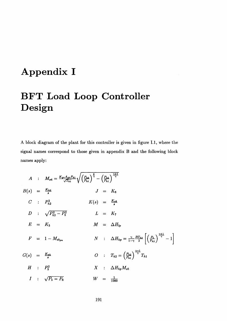
A ppendix I
B F T Load Loop Controller D esign
A block diagram of the plant for this controller is given in figure 1.1, where the
signal names correspond to those given in appendix B and the following block
names apply:
A Jl/f _ KgVAgvPhl■ M "* ~ VTm y l W -
(PhiV^i
V 2±i
) ’
B (s) _ *12 s J = Ke
C ■ P L K (s) = Kv 6s
D ■ V P L - P i L = k 7
E = K s M = A H lp
F = 1 Afsbpu N :
G(s) _ KvS s 0 :
H : P i X : XHhpMs§
I II w = i1000
191
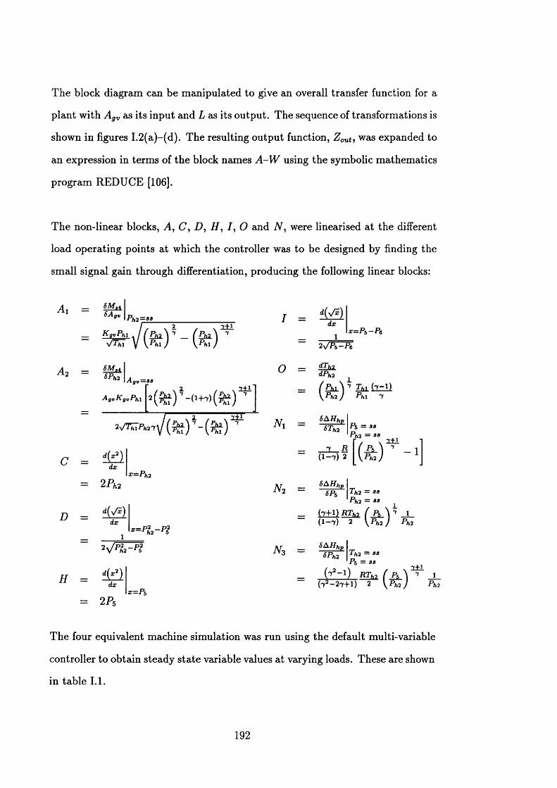
The block diagram can be m anipulated to give an overall transfer function for a
plant w ith Agv as its input and L as its output. The sequence of transformations is
shown in figures I.2(a)-(d). The resulting output function, Z out, was expanded to
an expression in terms of the block names A - W using the symbolic mathematics
program REDUCE [106].
The non-linear blocks, A, C, D , H , / , O and N , were linearised at the different
load operating points at which the controller was to be designed by finding the
small signal gain through differentiation, producing the following linear blocks:
Ax =
C =
D =
H =
wfk6A* I Ph2=ss I =_ d{y/x)
KjvPh1_y/Thi Pm ) ( \ xi± Phl) 7
Phi )
dx
1 x —Pb- P &
2
SPh 2 ■ "gv-
AgVKgvPhl
o = dTh7 dPh 2
( f t ) * - ( % )
2±17
2±T1
- (ft)’ Phi 7
Nx =SAHihp
d(x2)dx
2Ph2
- 7 R1 / \ 2±L 1
( f t ) ’ - •(1 -7 ) 2
x=Ph2
No
d y/x^dx
*=PL ~ P2
SAH hp SPs \T h2 = S S
Ph2 = ss
f r + 1 ) RTh2 ( Pb Y 1 ( 1 —7 ) 2 \P h 2 ) Pfi2
d(x2)
SAHhpSPh2 \^h2 = ss
'P5 = S3
dx
2 P5
RTih i
x=P$(72- 27+l) 2 (ft)
1±1 7 1
Ph2
The four equivalent machine simulation was run using the default multi-variable
controller to obtain steady state variable values at varying loads. These are shown
in table 1.1.
192
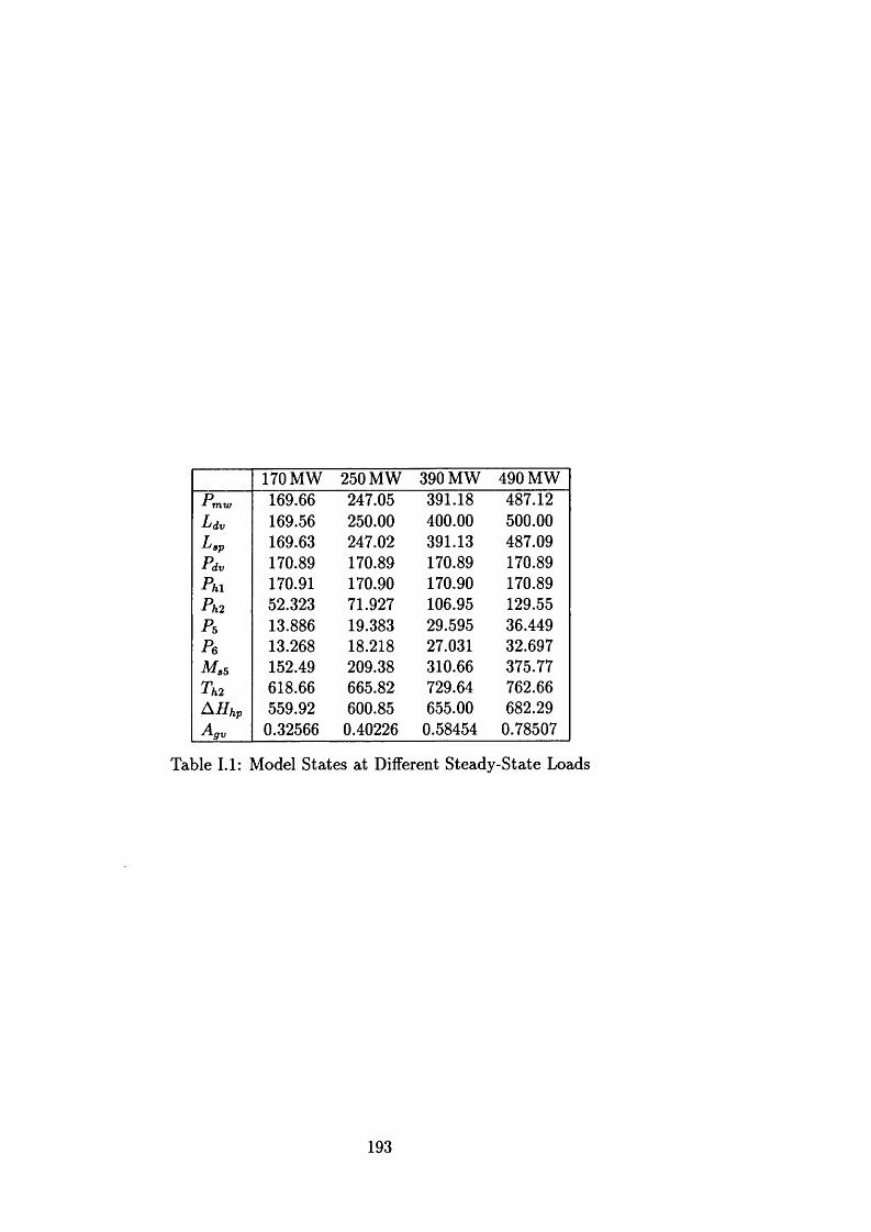
170 MW 250 MW 390 MW 490 MWp1 mw 169.66 247.05 391.18 487.12Ldv 169.56 250.00 400.00 500.00Pap 169.63 247.02 391.13 487.09Pdv 170.89 170.89 170.89 170.89Phi 170.91 170.90 170.90 170.89Ph2 52.323 71.927 106.95 129.55Ps 13.886 19.383 29.595 36.449Pe 13.268 18.218 27.031 32.697M a5 152.49 209.38 310.66 375.77Th2 618.66 665.82 729.64 762.66A Hhp 559.92 600.85 655.00 682.29Agy 0.32566 0.40226 0.58454 0.78507
Table 1.1: Model States at Different Steady-State Loads
193
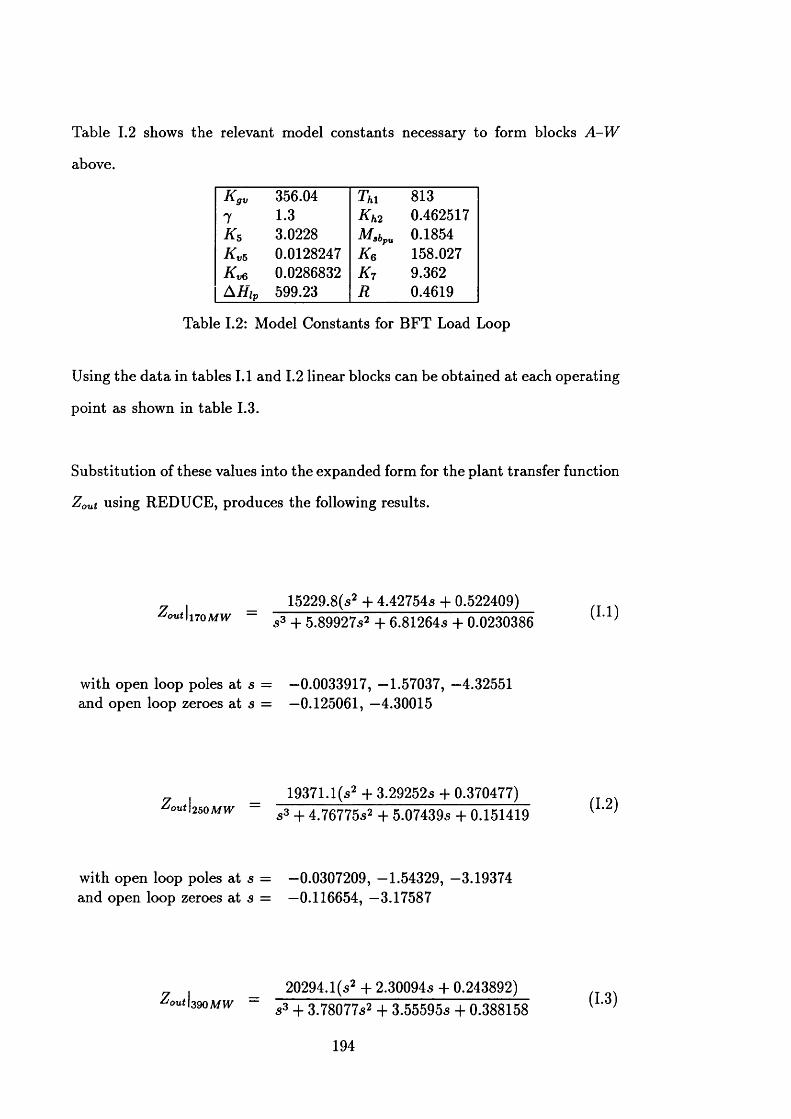
Table 1.2 shows the relevant model constants necessary to form blocks A - W
above.
K 9V 356.04 Th i 8137 1.3 K h2 0.462517k 5 3.0228 bpu 0.1854k v5 0.0128247 Ke 158.027Kys 0.0286832 k 7 9.362A H lp 599.23 R 0.4619
Table 1.2: Model Constants for B FT Load Loop
Using the d a ta in tables 1.1 and 1.2 linear blocks can be obtained at each operating
point as shown in table 1.3.
Substitution of these values into the expanded form for the plant transfer function
Z out using REDUCE, produces the following results.
15229.8(s2 -f 4.42754s + 0.522409)» « i l i 7 0 M W ~ 3 3 + 5 . 8 9 9 2 7 ^ 2 + 6.81264s + 0.0230386 ( ' ’
with open loop poles a t s = —0.0033917, —1.57037, —4.32551and open loop zeroes at s = —0.125061, —4.30015
19371. l ( s 2 + 3.292525 + 0.370477) 'outl^oMW ~ s3 + 4.76775s2 + 5.07439s + 0.1-51419
with open loop poles at s = —0.0307209, —1.54329, —3.19374 and open loop zeroes a t s = —0.116654, —3.17587
, _ 20294.1(s2 + 2.30094s + 0.243892)/°“i |39°w s 3 + 3 .7 8 0 7 7 s 2 + 3 .5 5 5 9 5 s + 0 .3 8 8 1 5 8 ( ' ’
194
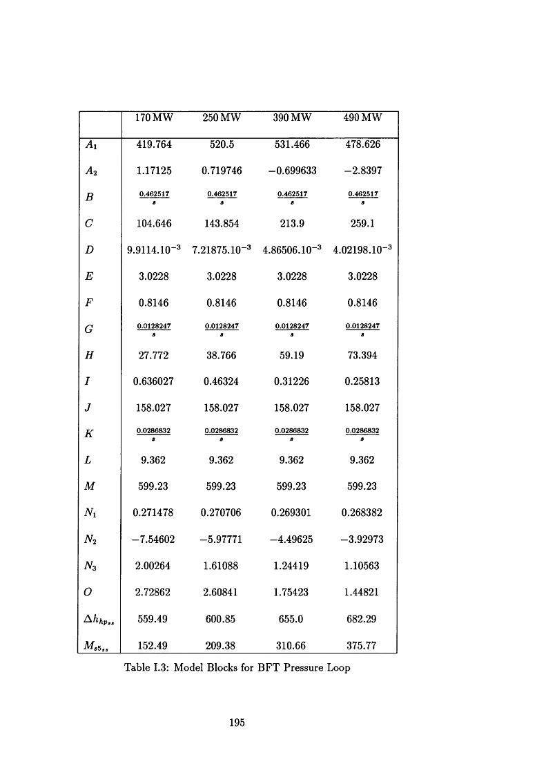
170 MW 250 MW 390 MW 490 MW
A i 419.764 520.5 531.466 478.626
A 2 1.17125 0.719746 -0.699633 -2.8397
B 0.462517a
0.4625178
0.462517a
0.462517a
C 104.646 143.854 213.9 259.1
D 9.9114.10-3 7.21875.10-3 4.86506.10“3 4.02198.10-3
E 3.0228 3.0228 3.0228 3.0228
F 0.8146 0.8146 0.8146 0.8146
G 0.01282478
0.01282478
0.0128247a
0.0128247a
H 27.772 38.766 59.19 73.394
I 0.636027 0.46324 0.31226 0.25813
J 158.027 158.027 158.027 158.027
K 0.02868328
0.0286832a
0.0286832a
0.0286832a
L 9.362 9.362 9.362 9.362
M 599.23 599.23 599.23 599.23
N r 0.271478 0.270706 0.269301 0.268382
n 2 -7.54602 -5.97771 -4.49625 -3.92973
n 3 2.00264 1.61088 1.24419 1.10563
0 2.72862 2.60841 1.75423 1.44821
^hfipss 559.49 600.85 655.0 682.29
M sbas 152.49 209.38 310.66 375.77
Table 1.3: Model Blocks for BFT Pressure Loop
195
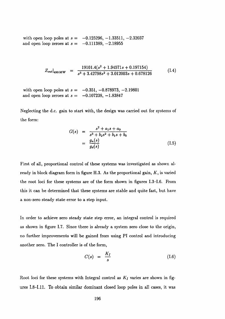
with open loop poles a t s = —0.125296, —1.33511, —2.32037and open loop zeroes a t s = —0.111389, —2.18955
19101.4(s2 + 1.94571s + 0.197154)»"<l49om w ~ s3 + 3.42798s2 + 3.012003s + 0.678126 ’
with open loop poles at s = —0.351, —0.878973, —2.19801 and open loop zeroes at s = —0.107238, —1.83847
Neglecting the d.c. gain to start with, the design was carried out for systems of
the form:
s2 + <ZiS + do s3 + 6 2s2 -J- b\S -f- 60
5” (s) (1.5)9d(s)
First of all, proportional control of these systems was investigated as shown al
ready in block diagram form in figure H.3. As the proportional gain, K , is varied
the root loci for these systems are of the form shown in figures 1.3-1.6. From
this it can be determined th a t these systems are stable and quite fast, but have
a non-zero steady state error to a step input.
In order to achieve zero steady state step error, an integral control is required
as shown in figure 1.7. Since there is already a system zero close to the origin,
no further improvements will be gained from using P I control and introducing
another zero. The I controller is of the form,
C (s) = ^ (1.6)s
Root loci for these systems with Integral control as K j varies are shown in fig
ures I.8-I.11. To obtain similar dominant closed loop poles in all cases, it was
196
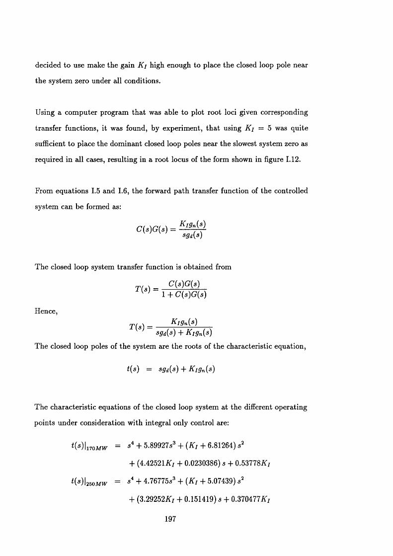
decided to use make the gain K i high enough to place the closed loop pole near
the system zero under all conditions.
Using a com puter program th a t was able to plot root loci given corresponding
transfer functions, it was found, by experiment, th a t using K i — 5 was quite
sufficient to place the dominant closed loop poles near the slowest system zero as
required in all cases, resulting in a root locus of the form shown in figure 1.12.
From equations 1.5 and 1.6, the forward path transfer function of the controlled
system can be formed as:
K ig n{s)C(s)G(s) =
sgd(s)
The closed loop system transfer function is obtained from
C (.)G ( .)W 1 + C(s)G(s)
Hence,
T(a) = Kl9n{s)sgd(s) + K Ign(s)
The closed loop poles of the system are the roots of the characteristic equation,
t(s) = sgd(s) + K Ign(s)
The characteristic equations of the closed loop system at the different operating
points under consideration with integral only control are:
< M li7 o w = s4 + 5.89927.S3 + ( # / + 6.81264) s 1
+ (4.42521.ft'j + 0.0230386) s + 0.53778 K ,
<(S)I25 0 W = s4 + 4.76775s3 + (K] + 5.07439) s2
+ (3.29252K i + 0.151419) a + 0.370477#/
197
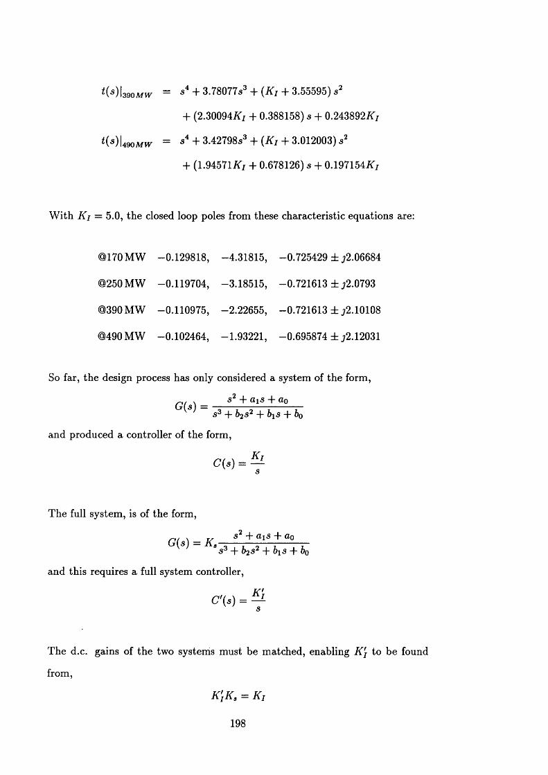
^ I s a o m w = s* + 3.78077s3 + (K , + 3.55595) s2
+ (2.30094A"/ + 0.388158) s + 0.243892A',
< W l49ow = s4 + 3.42798s3 + (K , + 3.012003) s2
+ (1.94571A'/ + 0.678126) 3 + 0.197154/0
W ith K i = 5.0, the closed loop poles from these characteristic equations are:
@170 MW -0.129818, -4.31815, -0.725429 ± ;2.06684
@250 MW -0.119704, -3.18515, -0.721613 ± j2 .0793
@390 MW -0.110975, -2.22655, -0.721613 ± ;2.10108
@490 MW -0.102464, -1.93221, -0.695874 ± ;2.12031
So far, the design process has only considered a system of the form,
> _ s2 + a is + Qp s3 + b2s2 + bis + b0
and produced a controller of the form,
C ( .) = ^ s
The full system, is of the form,
s2 T -}■ o>oG(s) = K as3 + b2s2 + bis + b0
and this requires a full system controller,
< ? ( . ) - &s
The d.c. gains of the two systems must be matched, enabling K j to be found
from,
K \ K a = K j
198
hence,
k ' - ^ l K i ~ K ,
This leads to the following controller gains required at each operating point,
@ 1 7 0 M W :# ; = 0.000328 @390 MW: K \ = 0.000246
@250 MW: K \ = 0.000258 @490 MW: = 0.000261
From root locus analysis, it was found th a t the positions of the dominant closed
loop poles were not very sensitive to the value of K i , or K j , at the design point.
Hence, it was considered th a t any value of K \ around the values calculated above
would do. Thus K j was chosen as,
K i = 0.00025
199

A ppendix J
Conversion o f Fossil M odel for Coal and for 660 M W U nits
J . l C reation o f C oal-F ired M od el
Coal-fired and oil-fired boilers are very similar in all aspects except for the fuel
system. Consequently, the only modification necessary to convert the original
oil-fired boiler model to coal-fired was to increase the tim e constants of the fuel
system, T/\ and T /2 to 40 and 20 seconds respectively instead of 15 and 5.
J .2 C reation o f 660 M W U n it M o d el
The original boiler model was for a 505 MW unit and a model was needed for a
667 MW unit. Certain assumptions were made in order to convert the 505 MW
model to a 667 MW model. The conversion is outlined below. Both model pa
ram eters and initial conditions of variables needed to be converted.
Firstly, it is assumed th a t the pressure conditions in the two sizes of unit will be
200
similar. Hence,-^667 ■ 605 = 174 bar
D1667 — P-*1505 = 167.6 bar
- 2667 - 2505 = 165.5 bar
D/ll667_ P-* 1505 = 163.3 bar
/l2667 Ph2sob = 107.9 bar
p1 5667 _ p-1 5505 = 29.88 bar
- 6667 ^6505 = 27.27 bar
Secondly, it is assumed th a t the tim e constants of the fuel supply systems are
similar. Hence, for a coal-fired boiler,
J/lMT = AVISOS = 40 SeC
T j2 „ 7 = Tf2S0S = 20 sec
Thirdly, it is assumed th a t fuel flow and steam flows are proportional to the unit
201
output power. Hence,
M f u667 = M f u ^ O b X 667505 = 2 3 . 9 4 9 x f § | = 3 1 . 6 3 2 m 3/se c
^ 6 6 7 = \ v 667 505 X 5Q5 = 2 3 . 9 4 9 x § § | = 3 1 . 6 3 2 m 3/se c
M s i 667 = ■^T»l505 X 6 67505
= 3 0 3 . 9 x g g = 4 0 1 . 3 9 m 3/se c
M Sp e67 = M ap 505 X 667505
= 9 . 5 x H I = 1 2 . 5 4 8 m 3/se c
M s 2 66 7 = M s 2s o s X 667505 = 3 1 3 . 4 x g = 4 1 3 . 9 4 m 3/se c
A fs3667 = M 3505 X 667505 = 3 1 3 . 4 x g g = 4 1 3 . 9 4 m 3/se c
M ^ s 4 667 = M a 4 5o s X 667505 = 3 1 3 . 4 x g g = 4 1 3 . 9 4 m 3/se c
M ^ s 5 667 = M s 5$ 05 X 667505 = 3 1 3 . 4 x f § | = 4 1 3 . 9 4 m 3/se c
M a b ^ 7 = M s b s o s X 667505 = 5 8 . 1 x g g = 7 6 . 7 3 8 m 3/se c
A /a 6 667 = M g 6505 X 667505 = 2 5 5 . 3 x g = 3 3 7 . 2 m 3/se c
M t s 7 §$7 = M a 7505 X 667505 = 2 5 5 . 3 x | § | = 3 3 7 . 2 m3/ sec
Assuming the same economiser outlet conditions and steam drum outlet condi
tions, means tha t,
hfde67 = hfds05 = 1284.00 k J/kg
h>667 = *>05 = 2532.32 k J/kg
An initial condition for boiler heat input can be found from
Q667 = M ai667 (h fd667 - hS667) = 501060 kJ/sec
Now,
^ = i [Q + Msl (h/d - fc.)]
Smaller units will respond more quickly to heat input changes, hence
^505 < ^667
202
Boiler tim e constants are in the approximate range of 250 sec-450 sec for boilers
ranging from 200 MW-660 MW. 0 wiU be assumed to vary in a similar proportion
even though it is not strictly the same thing. Hence, assuming a linear relation
ship between boiler tim e constant and unit size and using Tb to denote boiler
tim e constant,
This leads to,
TB" 7 = 250 + (TBm - 200) x ^
0667 — 0505 X-*■ Bsos
= 434078 x 1.1841
= 513992
Also,
K fure 67Q&67
^66750106031.632
= 15840.288
Using the basic model equations C.5, C.6 and C.7, other gains may now be found
as,K lm = lnM" mn— = 158.663
* * .» = /PM“% = 285.65V ^ e e r ^ * 6 6 7
= jp M'HJ p = 279-078y 2 6 6 7 ^ 1 667
Using equation C.8, K gv may be found from,
M aW T h i 1AgyPhl j / p ~7p \
V ( f c ) - ( & ) 7
203
Assuming the same physical conditions as before, ie. Thi = 813, 7 = 1.3 and
A gv = 0.7, then,
413.94 x v^13 1= --- — ------T— --- X
9 667 0.7 x 163.3 / / io7.9\i% / 107.9\V V 1 6 3 .3 / V 1 6 3 .3 /
= 470.265
Further gains may be found from equations C.9, C.10 and C .l l , thus,
K 5m7 = ,-------------- = 3.992667 / p2 p2
y h 2 6 6 7 5 6 67
K 6, , , = — = 208.726 6 7 “ f t , 6 6 7
k ^ t = 7 p “ - = 12.365®667
Reheat tim e constants range from approximately 9-16 seconds for unit sizes rang
ing from 200-660 MW. This implies a reheat time constant of 13.641 seconds for
a 505 MW unit and 16.107 seconds for a 667 MW unit. The gains relating steam
flow to pressure drop need to be smaller with increasing MW in the same ratio
as the reheat tim e constant. Hence,
1 1 T R m i
7 667 7 505 T R m
1= —— X 1.1808
Tv 505
T S 7 505_v T S ouo^ Km7 ~ l7l808
204
This leads to the following gains for the 667 MW model,
K vU67 = K v lm l . i m = 0.00749
K v2667 - K v2bQb 1.1808 = 0.00749
K h 166T = K Klm 1.1808 = 0.048816
Kh2es7 = Kh2sos 1.1808 = 0.391698
tft,5667 = ^55051-1808 = 0.010861
Kv6eer = t f * * . 1.1808 = 0.024291
Ld — Tj (M s5AH hp + M a7A H ip) -r-1000
Also assume,
^i266r — T,2605 — 738.86
and so,
663.18 k J/kg
Using,
Then,
Ai7/p667^ s 7 667
337.2
613.356 kJ/kg
205
A ppendix K
D igitisation o f Controllers
K .l S ym bols
(7(3) Controller Transfer Function
u(s) Laplace Transform of Controller O utput
e(s) Laplace Transform of System Error
K p Proportional Gain
K i Integral Gain
s Laplace Operator
T Digital Controller Time Interval
Uk Controller O utput at sample k
ek System Error a t sample Jc
206
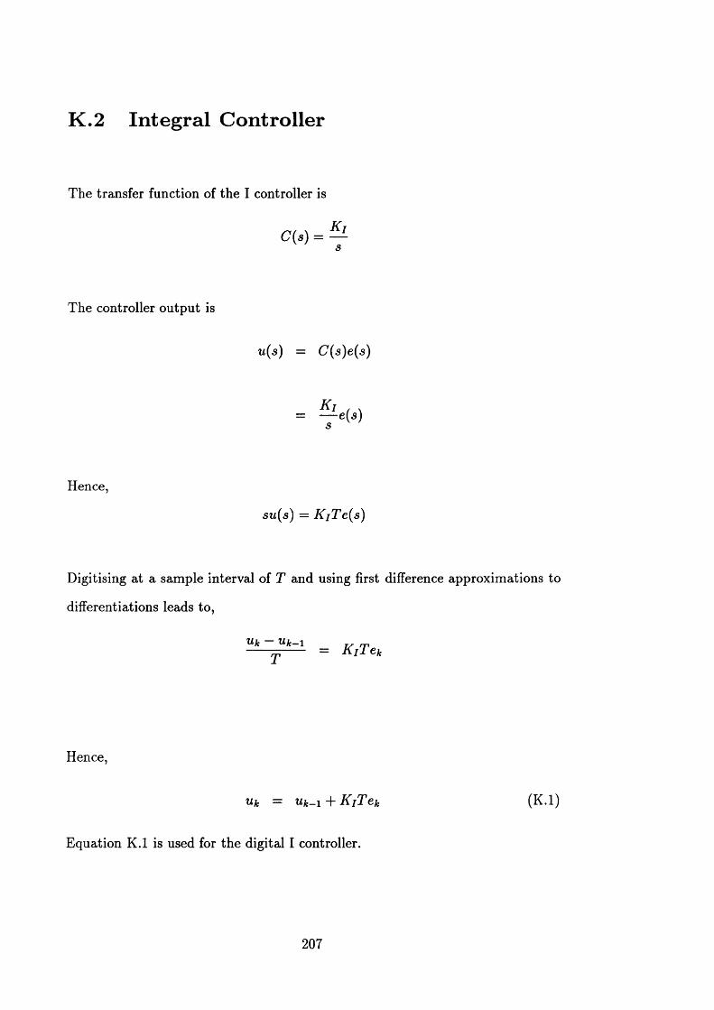
K .2 In tegral C ontroller
The transfer function of the I controller is
C(s) = s
The controller output is
Hence,
u(s) = C(.s)e(s)
K i f , = — e(s) s
su(s) = K jT e (s )
Digitising at a sample interval of T and using first difference approximations to
differentiations leads to,
Ulr Ulfc—1 m--- -■ ■ = K {T e k
Hence,
u k = Ufc-i + K {T e k (K .l)
Equation K .l is used for the digital I controller.
207
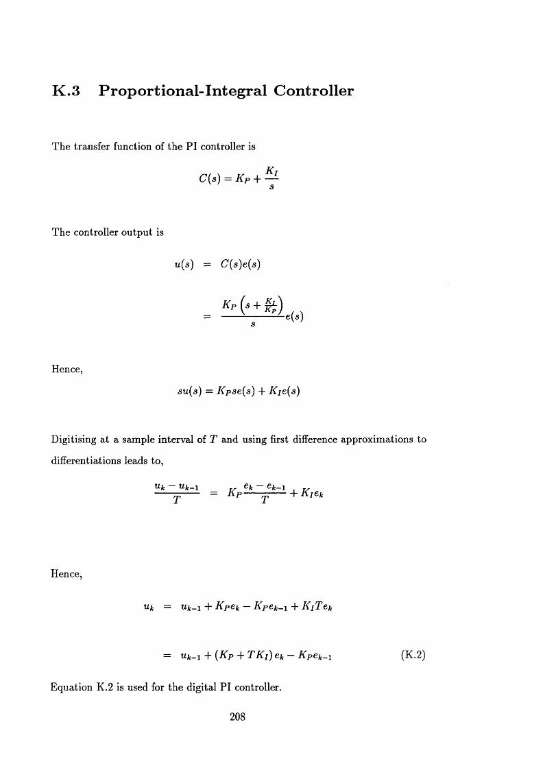
K .3 P rop ortion a l-In tegra l C ontroller
The transfer function of the P I controller is
C(s) = K P + — s
The controller output is
tt(s) = C(s)e(.s)
Hence,
su(.s) = Kpse(s) + K ie(s)
Digitising at a sample interval of T and using first difference approximations to
differentiations leads to,
^ k 1 j y Cfc— 1 j r
™----- = k p ----- ™------+ Ki^k
Hence,
Uk = U k ~ i + K p e k — K p e k - i + K i T e k
= Uk-i + ( K p + T K i ) e k — K p e k - i (K.2)
Equation K.2 is used for the digital PI controller.
208
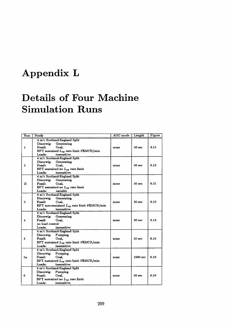
A ppendix L
D etails o f Four M achine Sim ulation R uns
Run Study AGC m ode Length Figure
1
4 m ’c Scotland-England Split Dinorwig: Generating Fossil: Coal,B F T sustained Lap rate lim it 5% M CR/min Loads: insensitive
none 50 sec 6.11
2
4 m ’c Scotland-England Split Dinorwig: Generating Fossil: Coal,B F T sustained no Lap rate lim it Loads: insensitive
none 50 sec 6.12
21
4 m ’c Scotland-England Split Dinorwig: Generating Fossil: Coal,B FT sustained no Lap rate lim it Loads: variable
none 50 sec 6.21
3
4 m ’c Scotland-England Split Dinorwig: Generating Fossil: Coal,B F T non-sustained Lap rate lim it 5% M CR/min Loads: insensitive
none 50 sec 6.13
4
4 m ’c Scotland-England Split Dinorwig: Generating Fossil: Coal, no load control Loewis: insensitive
none 50 sec 6.14
5
4 m ’c Scotland-England Split Dinorwig: Pum ping Fossil: Coed,B F T susteuned Lap rate lim it 5% M CR/min Loewis: insensitive
none 50 sec 6.15
5a
4 m ’c Scotlemd-Englemd Split Dinorwig: Pum ping Fossil: Coed,B F T susteuned Lap rate lim it 5% M CR/min Loads: insensitive
none 1000 sec 6.19
6
4 m ’c Scotland-England Split Dinorwig: Pumping Fossil: Coed,B F T sustained no Lap rate lim it Loewis: insensitive
none 50 sec 6.16
209
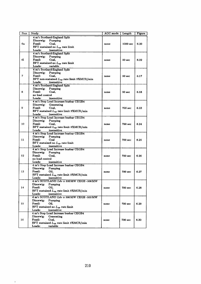
| Run | Study | AQC m ode | Length | Figure |
6a
4 m ’c Scotland-England Split Dinorwig: Pumping Fossil: Coal,B FT sustained no Lap rate lim it Loads: insensitive
none 1000 sec 6.20
61
4 m ’c Scotland-England Split Dinorwig: Pumping Fossil: Coal,B FT sustained no Lap rate lim it Loads: variable
none 50 sec 6.22
7
4 m ’c Scotland-England Split Dinorwig: Pumping Fossil: Coal,B F T non-sustained Lap rate lim it 5% M CR/min Loads: insensitive
none 50 sec 6.17
8
4 m ’c Scotland-England Split Dinorwig: Pumping Fossil: Coal, no load control Loads: insensitive
none 50 sec 6.18
9
4 m ’c Step Load Increase busbar CEGB4 Dinorwig: Generating Fossil: Coal,B FT sustained Lap rate lim it 5% M CR/min Loads: insensitive
none 700 sec 6.23
10
4 m ’c Step Load Increase busbar CEGB4 Dinorwig: Pumping Fossil: Coal,B FT sustained Lap rate lim it 5% M CR/min Loads: insensitive
none 700 sec 6.24
11
4 m ’c Step Load Increase busbar CEGB4 Dinorwig: Pum ping Fossil: Coal B FT sustained no Lap rate lim it Loads: insensitive
none 700 sec 6.25
12
4 m ’c Step Load Increase busbar CEGB4 Dinorwig: Pumping Fossil: Coal, no load control Loads: insensitive
none 700 sec 6.26
13
4 m ’c Step Load Increase busbar CEGB4 Dinorwig: Pum ping Fossil: Oil,B FT sustained Lap rate lim it 5% M CR/min Loads: insensitive
none 700 sec 6.27
14
4 m ’c SCOTLAND Ldv + 500 MW CEGB -500 MW Dinorwig: Pumping Fossil: Oil,B FT sustained Lap rate lim it 5% M CR/min Loads: insensitive
none 700 sec 6.28
15
4 m ’c SCOTLAND Ldv + 500 MW CEGB -500 MW Dinorwig: Pumping Fossil: Oil,BFT sustained no Lap rate lim it Loads: insensitive
none 700 sec 6.29
16
4 m ’c Step Load Increase busbar CEGB4 Dinorwig: Generating Fossil: Coal,B FT sustained Lap rate lim it 5% M CR/min Loads: variable
none 700 sec 6.30
210
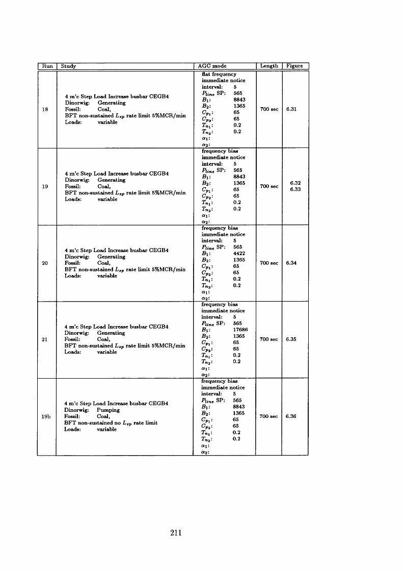
Run Study
4 m ’c Step Load Increase busbar CEGB4 Dinorwig: Generating
18 Fossil: Coal,B FT non-sustained Lap rate lim it 5% MCR/min Loads: variable
AGC m ode________flat frequency im m ediate notice
Length Figure
interval: 5Pline SP: 565Bn 8843B2: 1365CP l: 65Cpi' 65Tn i: 0.2Tt»3 : 0.2Ofi:a2:
700 sec 6.31
frequency bias im m ediate notice
4 m ’c Step Load Increase busbar CEGB4 Dinorwig: Generating
19 Fossil: Coal,B FT non-sustained L Sp rate lim it 5% MCR/min Loads: variable
interval: 5Pline SP: 565Bn 8843B2: 1365CPl: 65CP2: 65Tn i: 0.2Tn2: 0.2ori:a2:
700 sec 6.326.33
frequency bias im m ediate notice
4 m ’c Step Load Increase busbar CEGB4 Dinorwig: Generating
20 Fossil: Coal,B FT non-sustained Lap rate lim it 5% MCR/min Loads: variable
interval: 5Pline SP: 565Bn 4422B2: 1365Cp i : 65CP2: 65Tni: 0.2Tna: 0.2a i:a 2:frequency biasim m ediate noticeinterval: 5Pline SP: 565Bn 17686B2: 1365Cpi ’• 65Cp2: 65Tn i : 0.2I n j : 0.2
700 sec 6.34
4 m ’c Step Load Increase busbar CEGB4 Dinorwig: Generating
21 Fossil: Coal,B FT non-sustained Lap rate lim it 5% MCR/min Loads: variable
700 sec 6.35
ori: a 2:frequency bias im m ediate notice
4 m ’c Step Load Increase busbar CEGB4 Dinorwig: Pum ping
19b Fossil: Coal,B FT non-sustained no Lap rate lim it Loads: variable
interval: 5Pline SP: 565Bn 8843B2: 1365Cp i : 65CP2: 65Tni: 0.2Tn2: 0.2a na 2:
700 sec 6.36
211
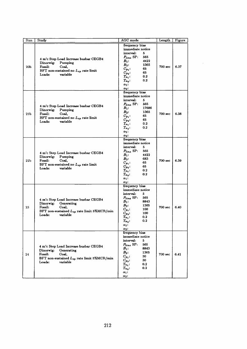
| Run | Study
4 m ’c Step Load Increase busbar CEGB4 Dinorwig: Pum ping
20b Fossil: Coal,B FT non-sustained no Lap rate lim it Loads: variable
AGC m odefrequency bias im m ediate notice
Length Figure
interval: 5Pline SP: 565Bn 4422B2: 1365C'P l: 65Cp a : 65Tn i: 0.2Tna: 0.2
700 sec 6.37
aila2i
4 m ’c Step Load Increase busbar CEGB4 Dinorwig: Pum ping
21b Fossil: Coal,B FT non-sustained no Lsp rate lim it Loads: variable
frequency bias im m ediate noticeinterval: 5Pline SP: 565Bn 17686B2: 1365Cp i ; 65Cp a : 65Tni: 0.2Tna: 0.2a na 2:frequency biasim m ediate noticeinterval: 5Pline SP: 565Bn 4422B2: 683Cp 65Cp3 : 65Tni: 0.2I n j : 0.2ana 2ifrequency biasim m ediate noticeinterval: 5Pline SP: 565Bn 8843B2 : 1365Cpi'. 100Cp?'- 100Tnn 0.2Tti^: 0.2
700 sec 6.38
4 m ’c Step Load Increase busbar CEGB4 Dinorwig: Pumping
22b Fossil: Coal,B FT non-sustained no Lap rate lim it Loads: variable
700 sec 6.39
4 m ’c Step Load Increase busbar CEGB4 Dinorwig: Generating
23 Fossil: Coal,B FT non-sustained Lap rate lim it 5% MCR/min Loads: variable
ai:0 2 :
700 sec 6.40
frequency bias im m ediate notice
4 m ’c Step Load Increase busbar CEGB4 Dinorwig: Generating
24 Fossil: Coal,B FT non-sustained Lap rate lim it 5% M CR/min Loads: variable
interval: 5Pline SP: 565Bi: 8843B2: 1365Cp i : 30CP3: 30Tni: 0.2Tna: 0.2ori:a 2:
700 sec 6.41
212
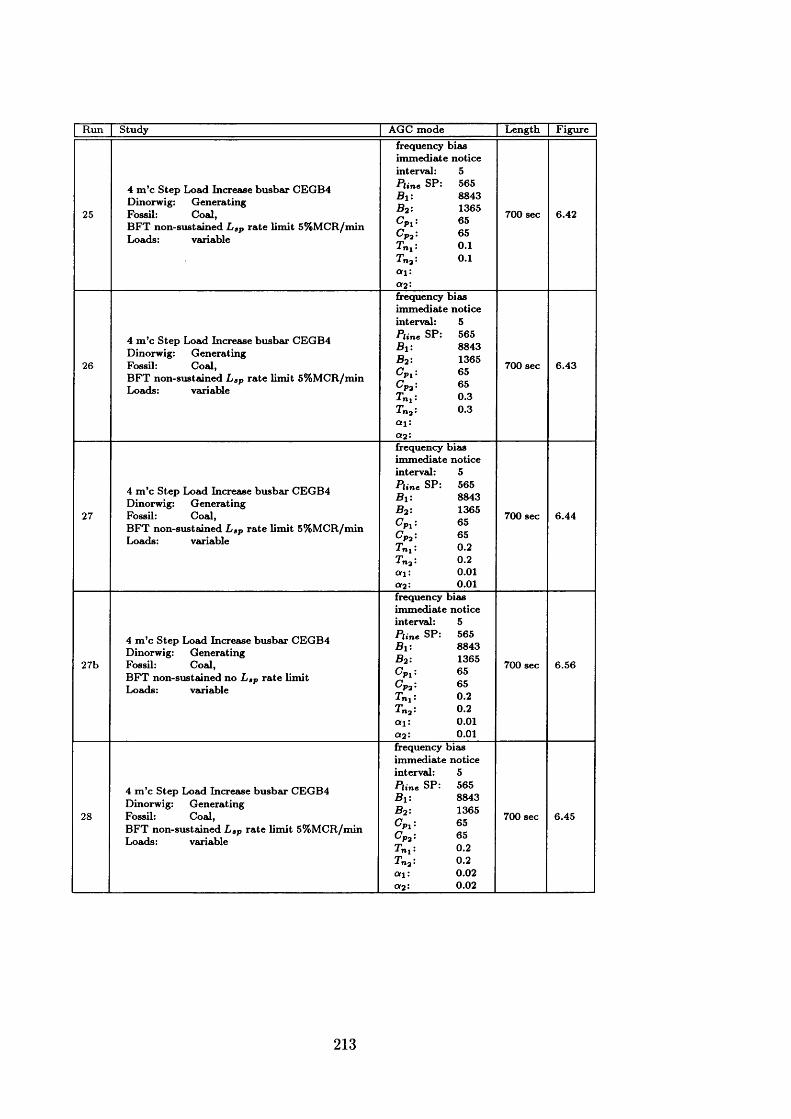
| Run | Study
4 m ’c Step Load Increase busbar CEGB4 Dinorwig: Generating
25 Fossil: Coal,B FT non-sustained L ap rate lim it 5% M CR/min Loads: variable
AGC m ode________frequency bias immediate notice
Length Figure
interval: 5Pline SP: 565By. 8843B2: 1365CPl: 65CP3: 65Tn i: 0.1Tr»3: 0.1ori:a y
700 sec 6.42
frequency bias im m ediate notice
4 m ’c Step Load Increase busbar CEGB4 Dinorwig: Generating
26 Fossil: Coal,B FT non-sustained Lap rate lim it 5% MCR/min Loads: variable
interval: 5Pline SP: 565By. 8843B2: 1365CP l: 65CP2: 65Tn i: 0.3Tna: 0.3
700 sec 6.43
ay.a yfrequency bias im m ediate notice
4 m ’c Step Load Increase busbar CEGB4 Dinorwig: Generating
27 Fossil: Coal,B FT non-sustained Lap rate lim it 5% MCR/min Loads: variable
interval: 5Pline SP: 565By. 8843By. 1365Cp i : 65Cp 3 : 65Tn i : 0.2Tn3: 0.2ot\: 0.01a y 0.01
700 sec 6.44
frequency bias im m ediate notice
4 m ’c Step Load Increase busbar CEGB4 Dinorwig: Generating
27b Fossil: Coal,B FT non-sustained no L sp rate lim it Loads: variable
interval: 5Pline SP: 565By. 8843B y 1365Cpi: 65CP3: 65Tn i : 0.2Tn3: 0.2o i: 0.01a y 0.01frequency biasim m ediate noticeinterval: 5Pline SP: 565By. 8843B y 1365Cp i ; 65CP2: 65Tni’. 0.2Tjj3 : 0.2ax: 0.02a y 0.02
700 sec 6.56
4 m ’c Step Load Increase busbar CEGB4 Dinorwig: Generating
28 Fossil: Coal,B FT non-sustained Lap rate lim it 5% MCR/min Loads: variable
700 sec 6.45
213
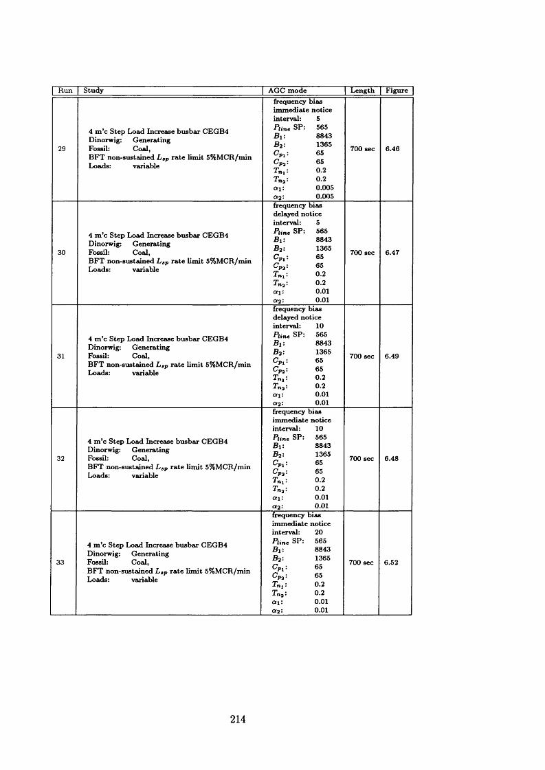
| Run | Study
4 m ’c Step Load Increase busbar CEGB4 Dinorwig: Generating
29 Fossil: Coal,B FT non-sustained Lap rate lim it 5% M CR/min Loads: variable
| AGC m odefrequency bias im m ediate notice interval: 5Pune SP: 565
Length I Figure
Bn 8843B2 : 1365CPi : 65CP2- 65Tni: 0.2
0.2ofj: 0.005<*2‘ 0.005
700 sec 6.46
frequency bias delayed notice
4 m ’c Step Load Increase busbar CEGB4 Dinorwig: Generating
30 Fossil: Coal,B FT non-sustained L ap rate lim it 5% M CR/min Loads: variable
interval: 5Pline SP: 565Bn 8843B2: 1365CPl: 65Cp3: 65Tni. 0.2Tna: 0.2an 0.01a2: 0.01frequency biasdelayed noticeinterval: 10Pline SP: 565Bn 8843B2: 1365Cp i : 65Cp 3 : 65Tnn 0.2Tn2: 0.2a n 0.01a 2: 0.01
700 sec 6.47
4 m ’c Step Load Increase busbar CEGB4 Dinorwig: Generating
31 Fossil: Coal,B FT non-sustained Lap rate lim it 5% MCR/min Loads: variable
700 sec 6.49
frequency bias im m ediate notice
4 m ’c Step Load Increase busbar CEGB4 Dinorwig: Generating
32 Fossil: Coal,B FT non-sustained Lsp rate lim it 5% M CR/min Loads: variable
interval: 10Pline SP: 565Bn 8843B2: 1365CP1: 65CP3: 65Tm: 0.2Tn2: 0.2a n 0.01a 2: 0.01frequency biasim m ediate noticeinterval: 20Pline SP: 565Bn 8843B2: 1365CPl: 65CP2: 65Tn i: 0.2Tn2: 0.2a n 0.01a 2: 0.01
700 sec 6.48
4 m ’c Step Load Increase busbar CEGB4 Dinorwig: Generating
33 Fossil: Coal,B FT non-sustained Lap rate lim it 5% MCR/min Loads: variable
700 sec 6.52
214
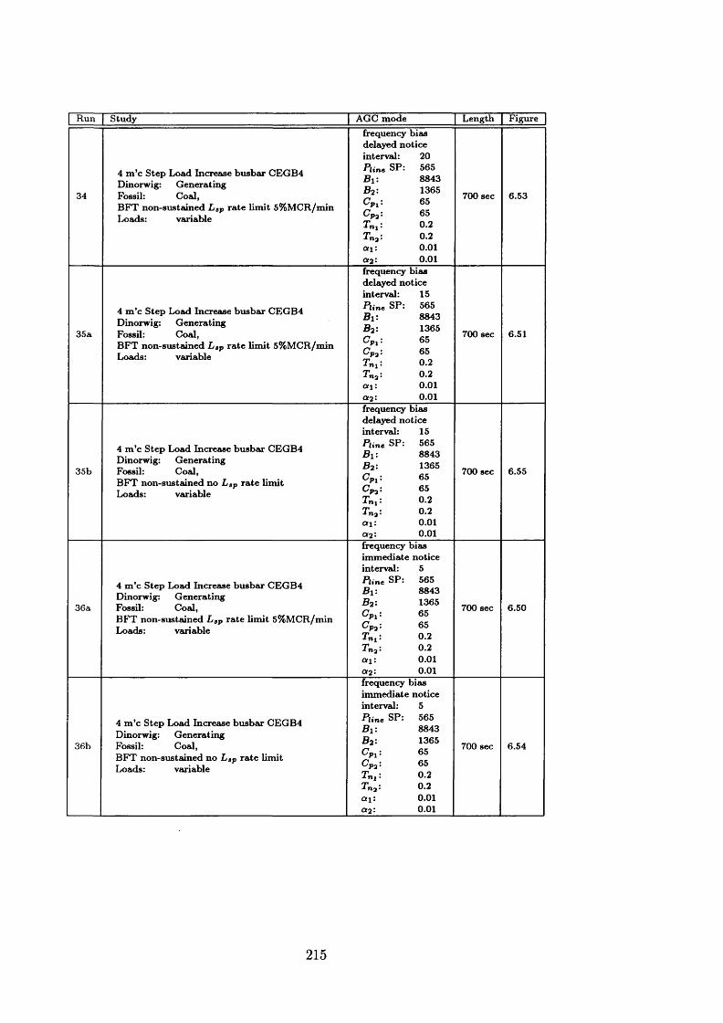
| Run | Study
4 m ’c Step Load Increase busbar CEGB4 Dinorwig: Generating
34 Fossil: Coal,B FT non-sustained Lap rate lim it 5% MCR/min Loads: variable
AGC m ode frequency bias delayed notice
Length Figure
interval: 20Pline SP: 565By. 8843By. 1365CPli 65Cp 2: 65Tn i : 0.2I n j ’ 0.2ay. 0.01a y 0.01frequency biasdelayed noticeinterval: 15Pline SP: 565By. 8843B y 1365CPl: 65Cp 3 : 65Tnx: 0.2I n j : 0.2Ofj: 0.010 2 : 0.01
700 sec 6.53
4 m ’c Step Load Increase busbar CGGB4 Dinorwig: Generating
35a Fossil: Coal,B FT non-sustained Lap rate lim it 5% M CR/min Loads: variable
700 sec 6.51
4 m ’c Step Load Increase busbar CEGB4 Dinorwig: Generating
35b Fossil: Coal,B FT non-sustained no Lap rate lim it Loads: variable
frequency biasdelayed noticeinterval: 15Pline SP: 565B y 8843B y 1365Cp i : 65Cpy. 65Tn\: 0.2Tn2: 0.2a i: 0.010 2 : 0.01
700 sec 6.55
frequency bias im m ediate notice
4 m ’c Step Load Increase busbar CEGB4 Dinorwig: Generating
36a Fossil: Coal,B FT non-sustained LSp rate lim it 5% MCR/min Loads: variable
interval: 5Pline SP: 565B y 8843B y 1365Cpy 65Cp?' 65Tnv: 0.2Tn2: 0.2a y 0.010 2 : 0.01frequency biasim m ediate noticeinterval: 5Pline SP: 565By. 8843B y 1365Cpi’. 65CP3: 65Tn i: 0.2Tn2: 0.2a y 0.010 2 : 0.01
700 sec 6.50
4 m ’c Step Load Increase busbar CEGB4 Dinorwig: Generating
36b Fossil: Coeil,B FT non-sustained no Lap rate lim it Loads: variable
700 sec 6.54
215
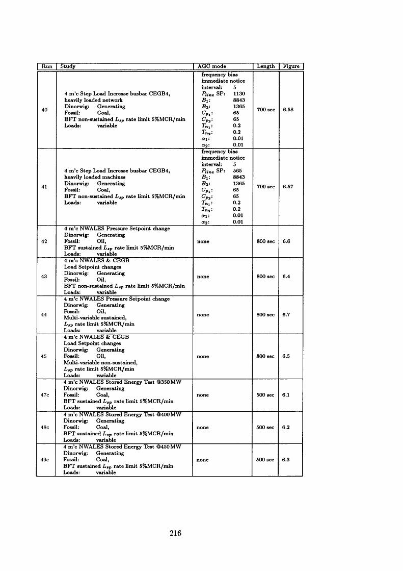
| Run | Study | AGC m ode Length Figure
40
4 m ’c Step Load Increase busbar CEGB4, heavily loaded network Dinorwig: Generating Fossil: Coal,B F T non-sustained L ap rate lim it 5% M CR/min Loads: variable
frequency bias im m ediate notice interved: 5 Pline SP: 1130 B i : 8843 B2: 1365 CPl: 65 CP2: 65 Tn i : 0.2 T„3: 0.2ori: 0.01 OT2’ 0.01
700 sec 6.58
41
4 m ’c Step Load Increase busbar CEGB4, heavily loaded machines Dinorwig: Generating Fossil: Coal,B FT non-sustained Lap rate lim it 5% MCR/min Loads: variable
frequency bias im m ediate notice interval: 5 Pline SP: 565 Bi: 8843 J92: 1365 0 P l: 65 Cp.,: 65 Tn i: 0.2 T„a: 0.2o i : 0.01 or2: 0.01
700 sec 6.57
42
4 m ’c NWALES Pressure Setpoint change Dinorwig: Generating Fossil: Oil,B FT sustained Lap rate lim it 5% M CR/min Loads: variable
none 800 sec 6.6
43
4 m ’c NWALES & CEGB Load Setpoint changes Dinorwig: Generating Fossil: Oil,BFT non-sustained Lap rate lim it 5% M CR/min Loads: variable
none 800 sec 6.4
44
4 m ’c NWALES Pressure Setpoint change Dinorwig: Generating Fossil: Oil,M ulti-variable sustained,Lap rate lim it 5% M CR/min Loads: variable
none 800 sec 6.7
45
4 m ’c NWALES & CEGB Load Setpoint changes Dinorwig: Generating Fossil: Oil,M ulti-variable non-sustained, Lap rate lim it 5% M CR/min Loads: variable
none 800 sec 6.5
47c
4 m ’c NWALES Stored Energy Test @350 MW Dinorwig: Generating Fossil: Coal,B FT susteuned Lap rate lim it 5% M CR/min Loads: variable
none 500 sec 6.1
48c
4 m ’c NWALES Stored Energy Test @400 MW Dinorwig: Generating Fossil: Coal,B FT sustained Lap rate lim it 5% M CR/min Loads: variable
none 500 sec 6.2
49c
4 m ’c NWALES Stored Energy Test @450 MW Dinorwig: Generating Fossil: Coal,B FT susteuned Lap rate lim it 5% M CR/min Loads: variable
none 500 sec 6.3
216

Run Study AGC m ode Length Figure
51
4 m ’c DINORWIG Manual Guide Vane Ramp, no frequency regulation Dinorwig: Generating Fossil: Coal,B FT sustained Lap rate lim it 5% M CR/min Loads: variable
none 20 sec 6.9
52
4 m ’c DINORWIG Response to Power Setpoint Increase Dinorwig: Generating Fossil: Coal,BFT sustained Lap rate lim it 5% M CR/min Loads: variable
none 100 sec 6.10
217
A ppendix M
D etails o f T w enty-F ive M achine Sim ulation R uns
Run Study25 m ’c Scotland-England Split Dinorwig: GeneratingFossil: Coal,B FT sustained L ap rate lim it 5% M CR/min Loads: variable
AGC m ode Length
100 sec
Figure
7.1
frequency bias im m ediate notice
25 m ’c Step Load Increase busbar EGGB4J Dinorwig: 1-6: Pum ping, LFR 40.00 Hz, 2.75 secs
10 Fossil: Coal,B FT susteuned Lap rate lim it 5% M CR/min Loads: variable
interval: 5Pline SP: 609By. 4208B2: 748Cp i : 65CP3: 65Tn i : 0.2Tn2: 0.2o i: 0.01a y 0.01
700 sec 7.2
frequency bias im m ediate notice
25 m ’c Step Load Increase busbar EGGB4J Dinorwig: 1-2: Generating, LFR 40.00 Hz 2.75 secs
3-6: Pum ping, LFR 40.00 Hz 2 .75secs Fossil: Coal,BFT susteuned L ap rate lim it 5% M CR/min Loetds: veiriable
interveil: 5Pline SP: 609B y 4208B y 748CP \ : 65CP2: 65Tnx: 0.2^nj • 0.2a y 0.01a 2: 0.01frequency bieusim m ediate noticeinterveil: 5Pline SP: 609B y 4208B y 748CP1: 65CP2 '■ 65Tnx: 0.2Tm • 0.2o i: 0.01a y 0.01
700 sec 7.3
25 m ’c Step Loetd Increase busbar EGGB4J Dinorwig: 1-2: Generating, LFR 40.00 Hz 2 .75secs
3-6: Pum ping, LFR 40.00 Hz 2 .75secs Fossil: Coal,som e B FT susteuned L ap rate lim it 5% M CR/min som e B FT susteuned L ap rate lim it 2% M CR/min Loads: variable
700 sec 7.4
218

Run Study
25 m ’c Step Load Increase busbar EGGB4J interval: 5Dinorwig: 1: Generating, LFR 49.85 Hz 2.75 secs Pline SP: 609
2: Generating, LFR 40 .00Hz 2.75 secs Bn 42083-6: Pum ping, LFR 40.00 Hz 2.75 secs B2: 748
Fossil: Coal, CP l: 65som e BFT sustained Lap rate lim it 5% M CR/min C7P3: 65som e BFT susteuned Lap rate lim it 2% M CR/min TB1: 0.2Loads: variable T n j: 0.2
cri: 0.01a 2: 0.01
AGC m ode frequency bias im m ediate notice
Length Figure
700 sec 7.5
219
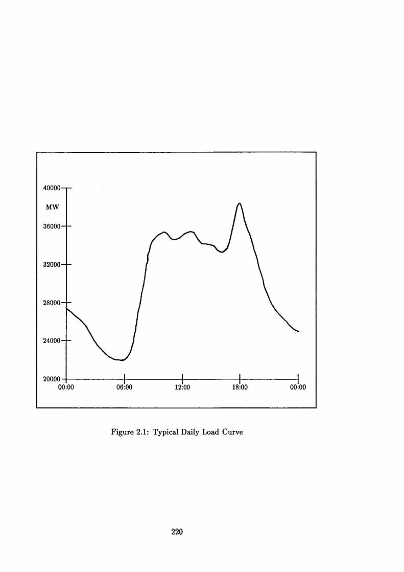
40000-r-
MW
36000
32000—
28000—
24000—
2000000:00 06:00 18:00 00:0012:00
Figure 2.1: Typical Daily Load Curve
220
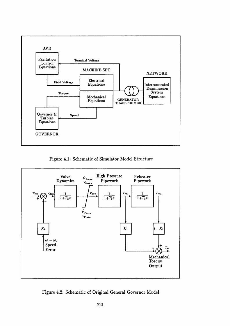
AYR
Terminal Voltage
MACHINE SETNETWORK
Field Voltage
Torque
GENERATORTRANSFORM ER
Speed
ExcitationControl
Equations
Governor &; Turbine
Equations
InterconnectedTransmission
SystemEquationsMechanical
Equations
ElectricalEquations
GOVERNOR
Figure 4.1: Schematic of Simulator Model Structure
ValveDynamics
High Pressure Pipework
ReheaterPipework
n»iP03
PminPmin
UJ — UJ,SpeedError
Mechanical Torque Output
Figure 4.2: Schematic of Original General Governor Model
221
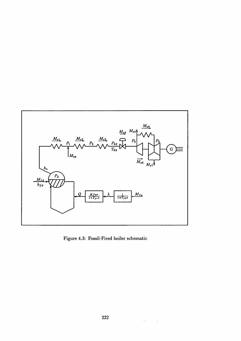
m ,6
•p«s
Figure 4.3: Fossil-Fired boiler schematic
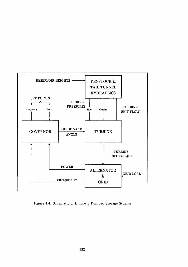
RESERVOIR HEIGHTS
SET POINTSTURBINE
PRESSURES TURBINE UNIT FLOW
PowerFrequency O utletInlet
GUIDE VANE
ANGLE
TURBINE UNIT TORQUE
POWER
GRID LOAD
FREQUENCY
GOVERNOR TURBINE
PENSTOCK k TAIL TUNNEL
HYDRAULICS
ALTERNATOR
GRID
Figure 4.4: Schematic of Dinorwig Pum ped Storage Scheme
223
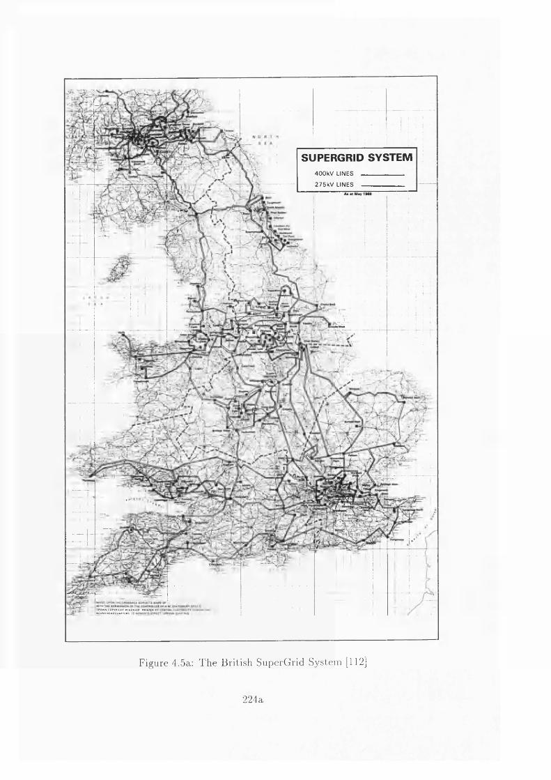
S U P E R G R I D S Y S T E M
400kV LINES275kV LINES
Figure 4.5a: The British SuperGrid System [112]
224a
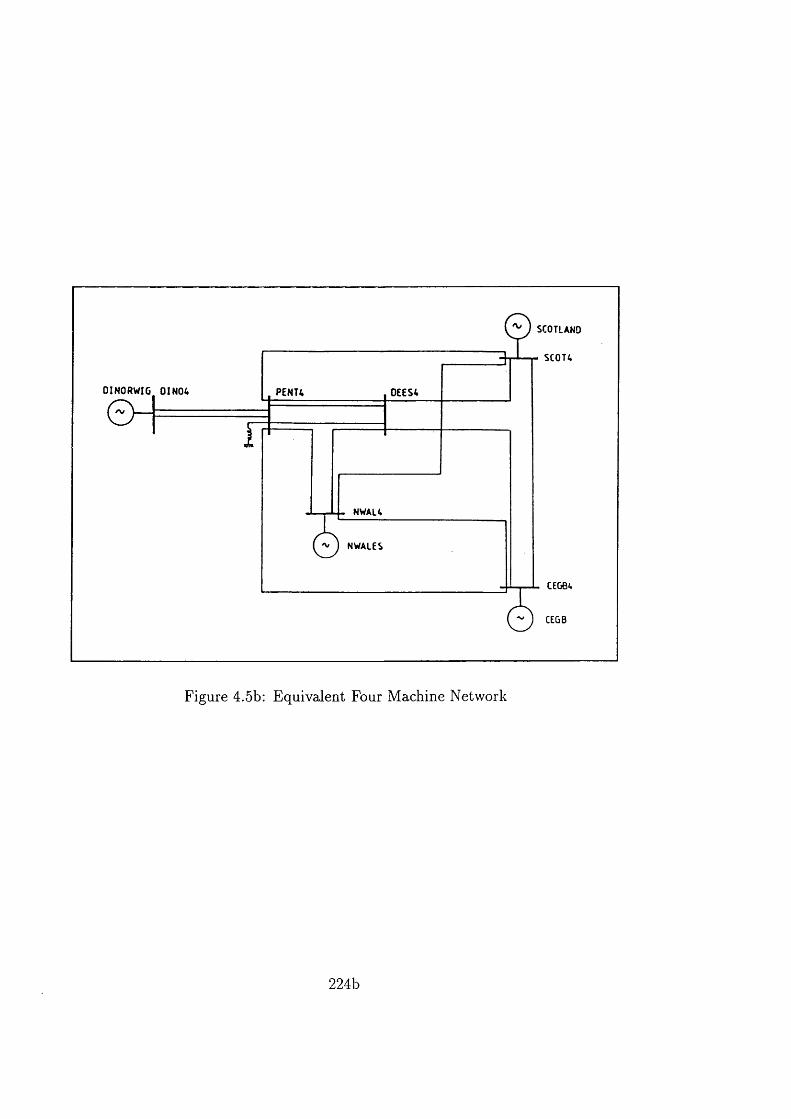
~ ) SCOTLAND
DINORWIG 0 I N 0 4 P E N U OEES4
NWALES
CEGB
Figure 4.5b: Equivalent Four Machine Network
224b
*dv
Turbine & Generator
Mills and Boiler
Grid
Figure 4.6: Typical Boiler Follows Turbine structure
225
GridTurbine & Generator
Mills and Boiler
Figure 4.7: Typical Turbine Follows Boiler structure
226
PhiM,MsMj
KeH )
F igure 4.8: Block D iagram of Fossil-Fired B oiler M odel
227
Figure 4.9: Block Diagram of BFT Pressure Loop PI Control
lgvG(s)
Figure 4.10: Block Diagram of BFT Load Loop I Control
228
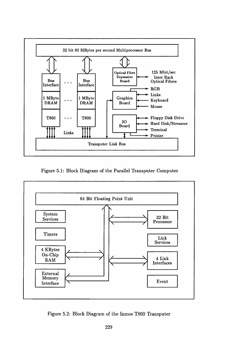
32 bit 80 MBytes per second Multiprocessor Bus
7S, 7S
Links
-----
Bus
________
BusInterface Interface
1 MByte 1 MByteDRAM DRAM
T800 T800
Optical Fibre Expansion
Board
GraphicsBoard
Board
Transputer Link Bus
125 Mbit/sec Inter Rack
Optical Fibres
RGBLinksKeyboardMouse
Floppy Disk Drive Hard Disk/Streamer Terminal Printer
Figure 5.1: Block Diagram of the Parallel Transputer Com puter
64 Bit Floating Point Unit
SystemServices 32 Bit
Processor
TimersLink
Services
4 K Bytes On-Chip
RAM 4 Link Interfaces
ExternalMemoryInterface Event
Figure 5.2: Block Diagram of the Inmos T800 Transputer
229
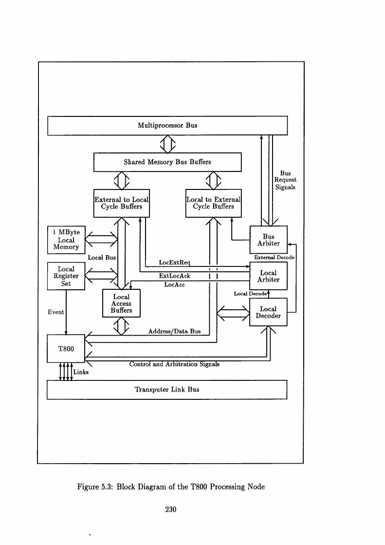
Multiprocessor Bus
x k .Shared Memory Bus Buffers
yv ' A X / \ /[ X\ /
_______ x t _______
External to Local-----------^ -----------Local to External
Cycle Buffers Cycle Buffers
Bus Request Signals
1 M Byte Local
MemoryBus
Arbiter
Local Bus External DecodeLocExtReq
Local Register
Set
LocalExtLocAck ArbiterLocAcc
Local DecodeLocalAccessBuffers LocalEvent Decoder
Address/Data Bus
Control and Arbitration SignalsLinks
Transputer Link Bus
Figure 5.3: Block Diagram of the T800 Processing Node
230
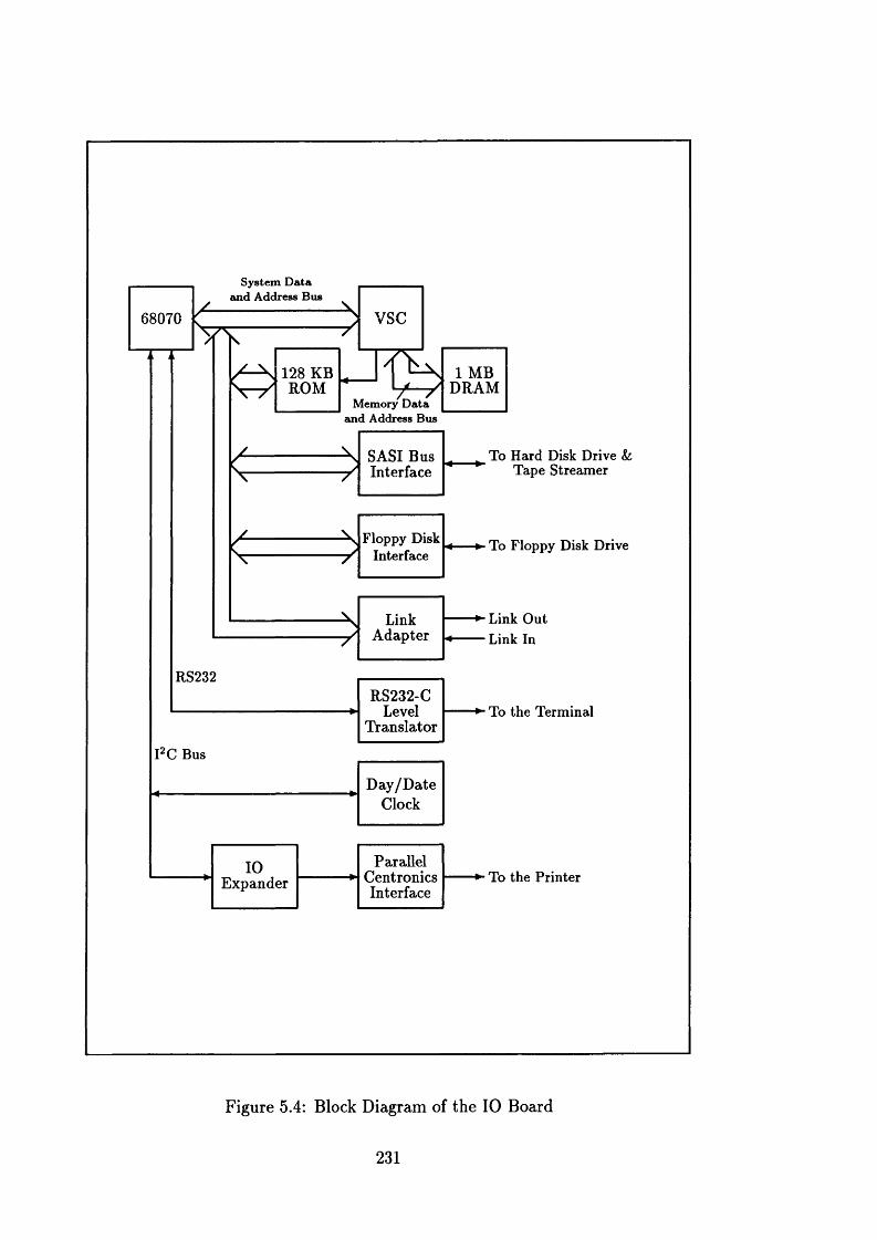
System D ata and Address Bus
vsc68070
128 KB ■V ROM
1 MB DRAM
Memory D ata and Address Bus
To Hard Disk Drive & Tape Streamer
SASI Bus - / Interface
Floppy Disk Interface
To Floppy Disk Drive
Link Out Link In
LinkAdapter
RS232RS232-C
LevelTranslator
To the Terminal
I2C Bus
D ay /D ateClock
ParallelCentronicsInterface
To the PrinterExpander
Figure 5.4: Block Diagram of the 10 Board
231
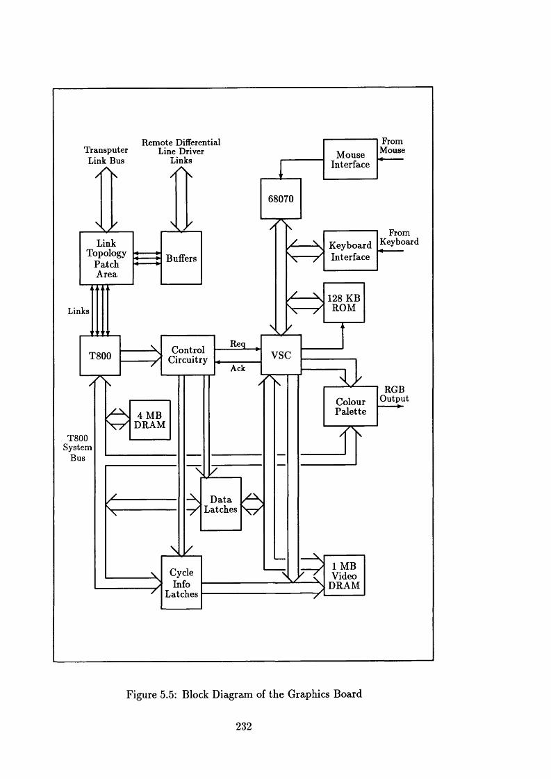
Transputer Link Bus
yv A N
\ / /Link
TopologyPatchArea
Links
Remote Differential Line Driver
Links y\
A N
Buffers
N
V
V
T800
s \A N
yControl
Circuitry
T800System
Bus
4 MB DRAM
V
N
y
N
y
Req
Ack
y
D ataLatches \
1/
CycleInfo
Latches
VSC
7K\
MouseFrom
Mouse
Interface
68070
TKeyboardInterface
FromKeyboard
y128 KB ROM
\ /V RGBColour OutputPalette
I T T\y
1 MB Video
DRAM
Figure 5.5: Block Diagram of the Graphics Board
232
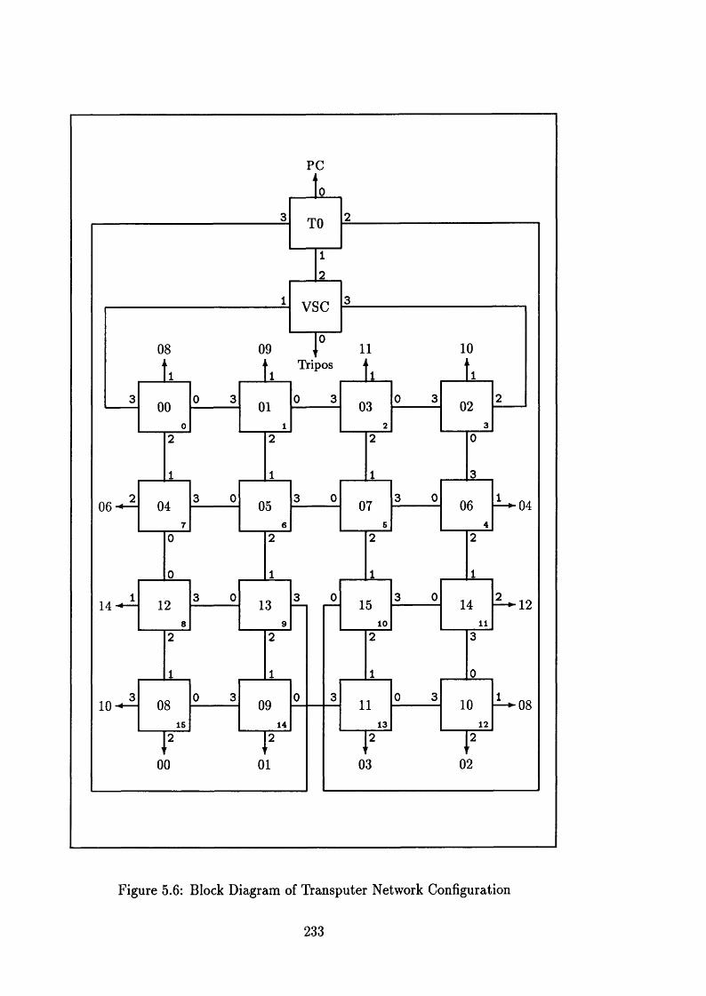
PC
Tripos
10
15 13
TO
14
vsc
Figure 5.6: Block Diagram of Transputer Network Configuration
233
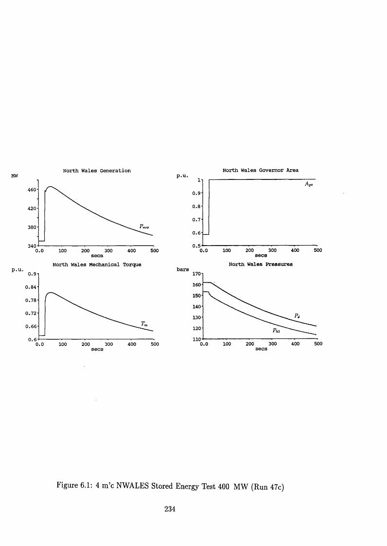
North Wales Generation North Wales Governor Area
460-
420-
380-
3405004000.0 100 200 300secs
North Wales Mechanical Torque0.9-1
0 .8 4 -
0 .78 -
0 .7 2 -
0.66-
0.65004000.0 100 200 300
0 .9
0.8-
0 .7
0.6-
0 .5500200 300 4001000.0 secs
North Wales Pressuresbars
170-1
160
150-
140
130-
120 Phi110
500300 400100 2000.0
Figure 6.1: 4 m ’c NWALES Stored Energy Test 400 MW (Run 47c)
234
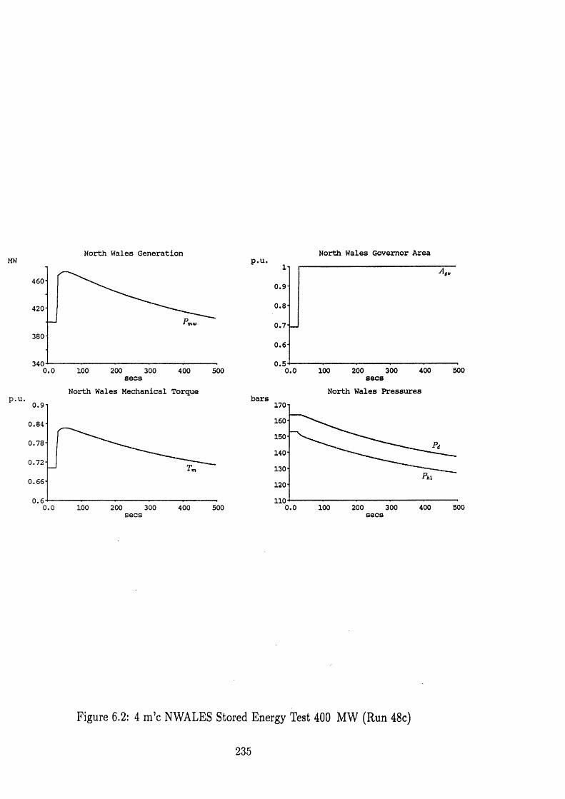
MW
p.U.
North Wales Generation
460-
420-
380-
3400.0 100 200 300 400 500secsNorth Wales Mechanical Torque
0.9n
0 .84-
0 .78-
0.60.0 100 200 300 400 500
North Wales Governor Areap . u .
Igy
0 .9 -
0.8-
0 .7 -
0.6-
0 .5500400200 3000.0 100 secs
North Wales Pressuresbars
170
160
150
140
130Phi
120110
500300 4000.0 100 200
Figure 6.2: 4 m ’c NWALES Stored Energy Test 400 MW (Run 48c)
235
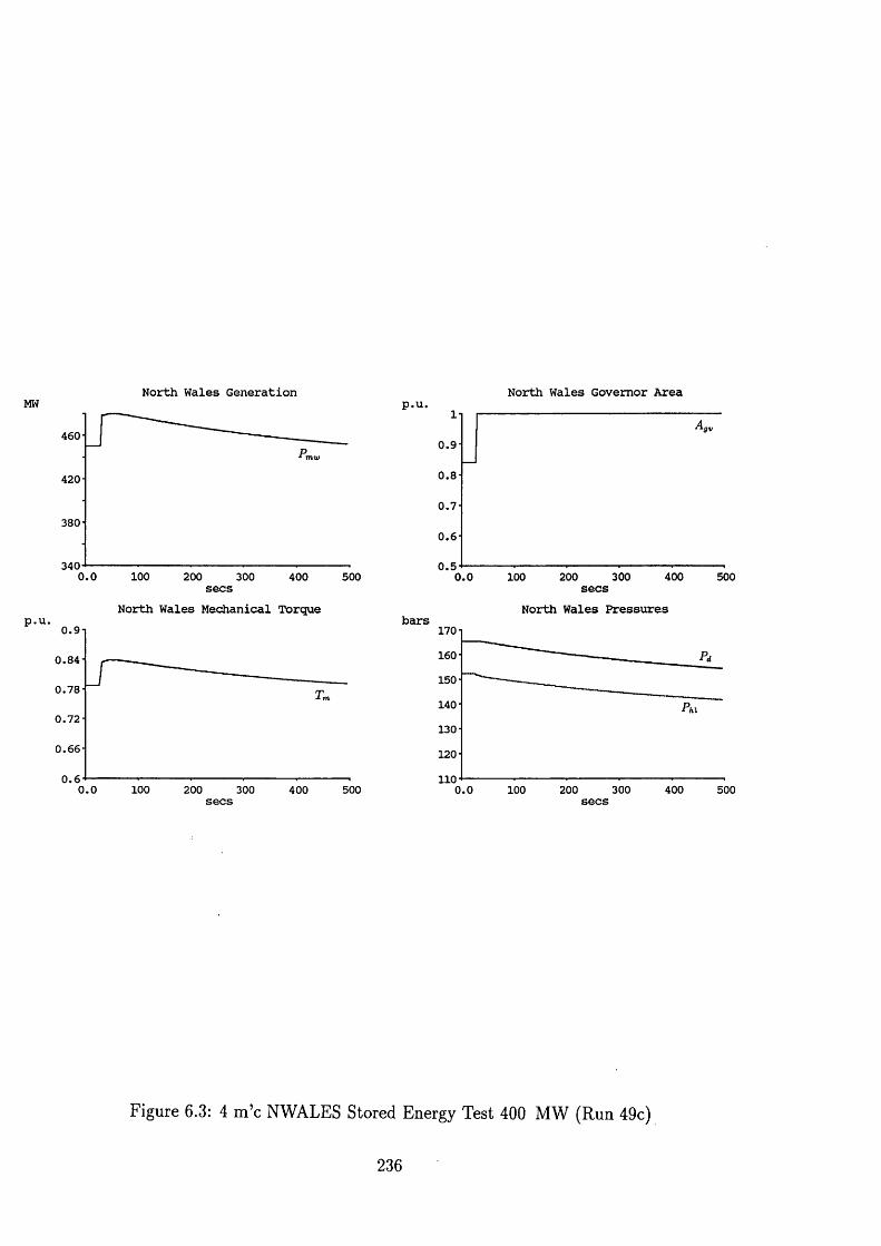
North Wales Generation North Wales Governor Area
4 6 0
4 2 0
3 8 0
3 4 00.0 100 200 3 00 4 0 0 5 0 0secs
North Wales Mechanical Torque0 .9 - i
0 .8 4 -
0 .7 8 -
0 .7 2 -
0.66-
0.60.0 100 200 300 5004 0 0
0 .9 -
0.8-
0 .7 -
0.6-
0 . 53 00 4 0 0 5000.0 100 200
secsNorth Wales Pressuresbars
170
16 0
150
140
130
120110
40 0100 200 3 00 50 00.0
Figure 6.3: 4 m ’c NWALES Stored Energy Test 400 MW (Run 49c)
236

( \ f \ L

Tie-Line PowerMW585
580
575
570line
565
560
0.0 200 400 600 800secs
SCOTLAND FrequencyHz50
4 9 .9 8
4 9 .9 6
4 9 .9 4
4 9 .9 2
4 9 .90.0 200 400 600 800
CEGB FrequencyHz50
ceg
49 .9 8
4 9 .9 6
4 9 .9 4
49 .92
4 9 .90.0 200 400 600 800
CEGB Generation SCOTLAND GenerationMW
MW
465
462
459
456
453
4500.0 200 400 600 800secs
DINOKWIG Generation195
190
185
180
175
170
165600 8000.0 200 400
MW
MW
368
366
364
362
360
3580 . 0 400 600200 800
secsNWALES Generation
480
'4p,440
400
360
3200.0 200 400 600 800
Figure 6.4: (a) 4 m ’c NWALES and CEGB Load Setpoint Changes (Run 43)
237
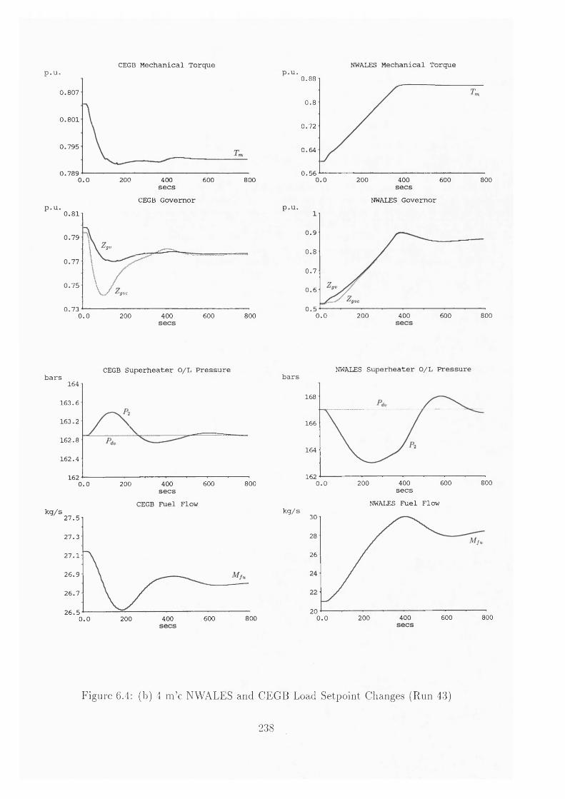
CEGB Mechanical Torque NWALES Mechanical Torquep.u. p.u.
0 .8 0 7
0 .8 0 1
0 .7 9 5
0 .7 8 90.0 200 400 600 800
p.u.
secs CEGB Governor
0 .8 1
0 .7 9Igv
0 .7 7
0 .7 5Igvc
0 .7 3400 600 8000.0 200
0.88
0 . 8
0 .7 2
0 .6 4
0 .5 60.0 200 400 600 800
p.U.
secs NWALES Governor
0 .9
0.8
0 .7
0 . 6
0 .50.0 200 400 600 800
barsCEGB Superheater O/L Pressure
164
16 3 .6
163 .2
16 2 .8
16 2 .4
162600 8000.0 200 400
kg/s
secs CEGB Fuel Flow
2 7 .5
2 7 .3
2 7 .1
2 6 .9
2 6 .7
2 6 .5600 800200 4000 . 0
barsNWALES Superheater O/L Pressure
kg/s
168
166
164
162800400 6000.0 200
secsNWALES Fuel Flow
30
28
26
20600 8004000.0 200
Figure 6.4: (b) 4 m ’c NWALES and CEGB Load Setpoint Changes (Run 43)
238
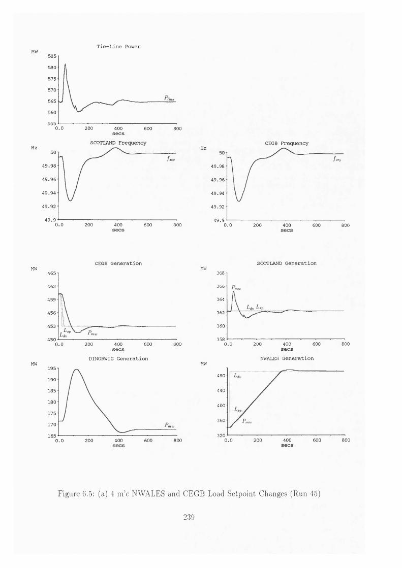
Tie-Line PowerMW585
580
575
570
565
560
5550.0 200 400 600 800secs
SCOTLAND FrequencyHz
50
4 9 .9 8
4 9 .9 6
4 9 .9 4
4 9 .9 2
4 9 .90.0 200 400 600 800
CEGB FrequencyHzceg
4 9 .98
4 9 .9 6
4 9 .94
4 9 .92
4 9 .90.0 200 400 600 800
CEGB Generation SCOTLAND GenerationMW
MW
465
462
459
456
453
450600 8000.0 200 400
secsDINORWIG Generation
195
190
185
180
175
170
165400 600 8000.0 200
MW
MW
368
366
364
362
360
3588000.0 200 400 600
secsNWALES Generation
480
440
400
360
320400 600 8000.0 200
Figure 6.5: (a) 4 m’c NWALES and CEGB Load Setpoint Changes (Run 45)
239

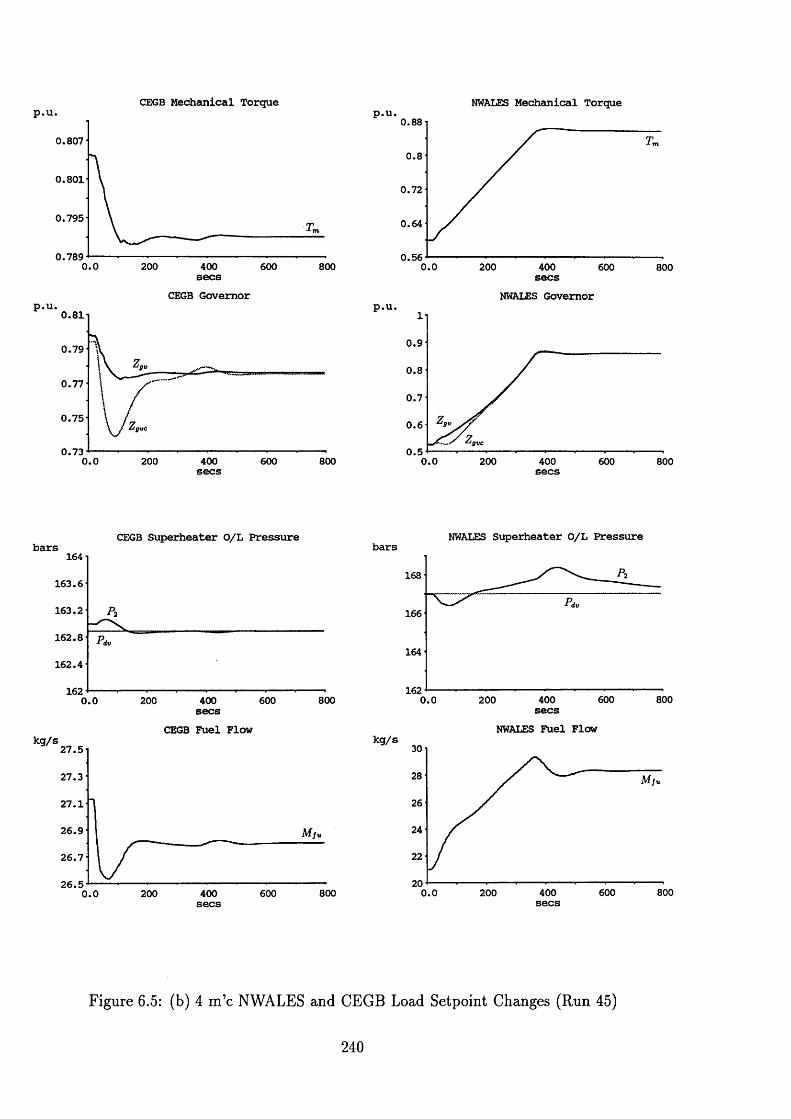
CEGB Mechanical Torque NWALES Mechanical Torquep.u. p.u.
0 .807
0 .801
0 .795
0 .7890.0 200 400 600 800
p.u.
secs CEGB Governor
0 .8 1
0 .7 9lgv
0 .7 7
0 .7 5tgvC
0 .7 3400 8000.0 200 600
0.88
0.8
0.72
0.64
0 .560.0 200 400 600 800
p.u.
secs NWALES Governor
0 .9
0.8
0 .7
0.6
0 .50.0 200 400 600 800
barsCEGB Superheater O/L Pressure
164
163 .6
163.2
162 .8
162.4
162800200 400 6000.0
kg/s
secs CEGB Fuel Flow
2 7 .5
27 .3
2 7 .1
2 6 .9
2 6 .7
2 6 .5800400 6000.0 200
bars NWALES Superheater O/L Pressure
168
P<tv166
164
162600 800200 4000.0 secs
NWALES Fuel Flowkg/s
22
20600 800200 4000.0
Figure 6.5: (b) 4 m ’c NWALES and CEGB Load Setpoint Changes (Run 45)
240

A : o
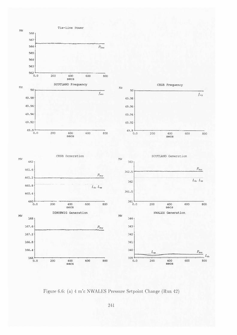
Tie-Line PowerMW568
567
566
565
564
563
5620.0 200 400 600 800
Hz
secsSCOTLAND Frequency
50
49.98
4 9 .9 6
4 9 .9 4
49.92
4 9 .90.0 200 400 600 800
Hz CEGB Frequency50
ceg
4 9 .9 8
4 9 .9 6
49 .9 4
49 .92
4 9 .90.0 200 400 600 800
CEGB Generation SCOTLAND GenerationMW
MW168
1 6 7 .6
1 6 7 .2
1 6 6 .8
1 6 6 .4
1660.0
462
4 6 1 .6
4 6 1 .2
4 6 0 .8
4 6 0 .4
4600.0 200 400 600 800secs
DINOKWIG Generation
200 400secs
600 800
MW363
3 6 2 .5
362
3 6 1 .5
3610.0 200 400 600 800
MW
secsNWALES Generation
344
343
342
341
340'»p
3390.0 200 400 600 800
Figure 6.6: (a) 4 m ’c NWALES Pressure Setpoint Change (Run 42)
241

Q't' (p . (c? ( c £ )
CEGB Mechanical Torque NWALES Mechanical Torquep.u.
0 .8 1
0 .8 0 8
0 .8 0 6
0 .8 0 4
0 .8 0 2
0.80.0 200 400 600 800
p.U.
secs CEGB Governor
0 .8 0 2 5
0 .8 0 2
0 .8 0 1 5
0 .8 0 1 'gvc
0 .8 0 0 5
0 . 8600 8000.0 200 400
p.u.0 .6 0 5
0 .6 0 3
0 .6 0 1
0 .5 9 9
0 .5 9 70.0 200 400 600 800
p.u
secs NWALES Governor
0 .5 4
0 .5 3 6
0 .5 3 2
'gvc0 .5 2 8
0 .5 2 4
0 .5 2400 600 8000.0 200
barsCEGB Superheater O/L Pressure
164
1 6 3 .6
1 6 3 .2
1 6 2 .8
1 6 2 .4
162800400 6000.0 200
kg/s
secs CEGB Fuel Flow
2 7 .5
2 7 .3
2 7 .1
2 6 .9
2 6 .7
2 6 .5800400 6002000.0
barsNWALES Superheater O/L Pressure
168
166
164
162400 600 8002000.0
kg/s
secsNWALES Fuel Flow
21.6
21 .2
20
20.4
20 800400 6000.0 200
Figure 6.6: (b) 4 m ’c NWALES Pressure Setpoint Change (Run 42)
242

'jfL O o )
Tie-Line PowerMW 568567
line
566
565
564
563
5620.0 200 400 600 800
Hz
secs3COTIAND Frequency
50
4S.98
49.96
49.94
49.92
49.90.0 200 400 600 800
CEGB GenerationMW 462
461.6
461.2
460.8
460.4
4600.0 200 400 600 800secsDINOEWIG GenerationMW 168
167.6
167.2
166.8
166.4
1660.0 200 400 600 800
HZ CEGB Frequency
ceg
49.98
49.96
49.94
49.92
49.90.0 200 400 600 800secs
SCOTLAND GenerationMW 363
362.5
362
361.5
3610.0 200 400 600 800secsNWALES GenerationMW 344
343
342
341
340
339 4000.0 200 600 800secs
Figure 6.7: (a) 4 m ’c NWALES Pressure Setpoint Change (Run 44)
243

W U .No, (o •'1 ( £ 0
p.u. CEGB Mechanical Torque0 .8 1
0 .8 0 8
0 .8 0 6
0 .8 0 4
0 .8 0 2
0 .80 .0 200 400 600 800
secs CEGB Governor
0 .8 0 2 5
0 .8 0 2'gv
0 .8 0 1 5
0 .8 0 1'gvc
0 .8 0 0 5
0 . 80.0 200 400 600 800
p.U. NWALES Mechanical Torque
0 .6 0 5
0 .6 0 3
0 .6 0 1
0 .5 9 9
0 .5 9 70.0 200 400 600 800secs NWALES Governorp.u
0 .5 4
0 .5 3 6
*gv0 .5 3 2
'gvc0 .5 2 8
0 .5 2 4
0 .5 20.0 200 400 600 800secs
bars CEGB Superheater O/L Pressure164
1 6 3 .6
1 6 3 .2
1 6 2 .8
1 6 2 .4
162
P i
Pdv
kg/s
0 .0 200 400 600secs
CEGB Fuel Flow
800
2 7 .5
2 7 .3
2 7 .1
2 6 .9
2 6 .7
2 6 .5200 400 600 8000 .0
barsNWALES Superheater O/L Pressure
168
166
164
1620.0 200 400 600 800secs
NWALES Fuel Flowkg/s
21.6
21.2
20.8
2 0 .4
8000 .0 200 400 600secs secs
Figure 6.7: (b) 4 m ’c NWALES Pressure Setpoint Change (Run 44)
244
o r q u e / S P e e d c
T 1 1
6 0
D i s c h a r g e / S p e e d C
20
6 0
Figure 6.8
245

nJ
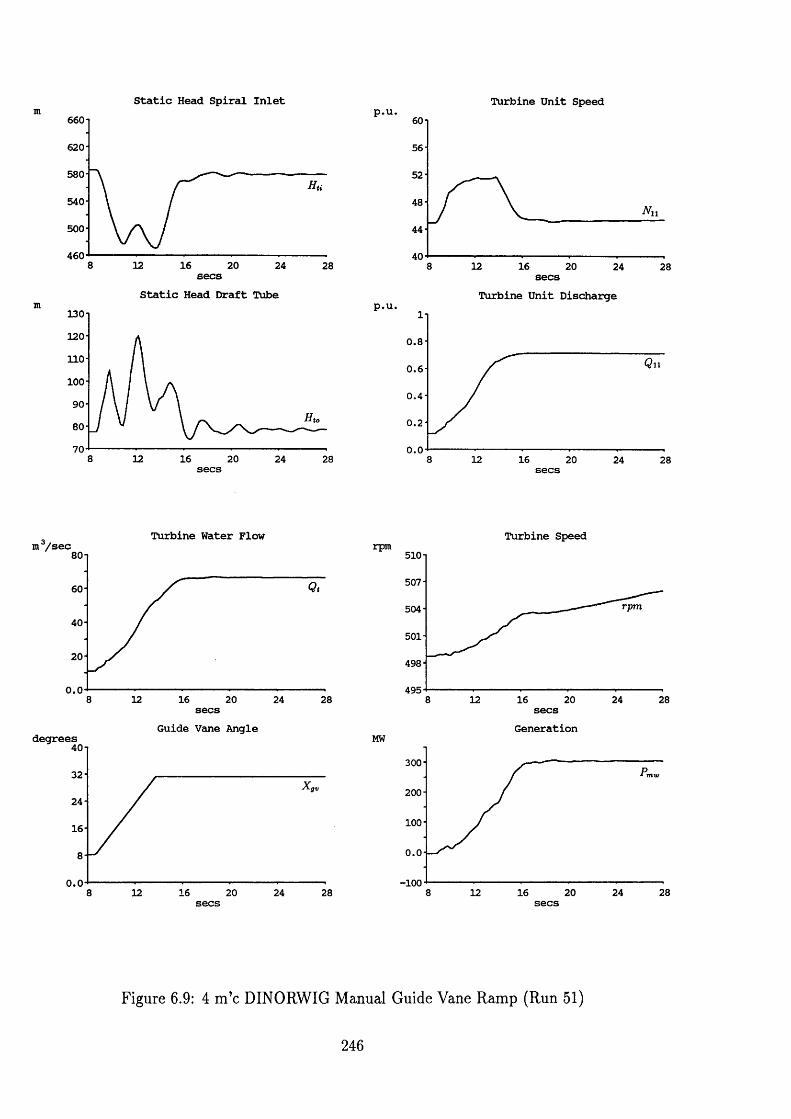
Static Head Spiral Inlet660 t
620
580
540
500
460 8 12 16 20 24 28secsStatic Head Draft Tube
130-]
120-
n o -
100-90-
80-
70 8 12 16 20 24 28
p .U .Turbine Unit Speed
60-1
56-
52-
48-
40128 16 20 24 28
p .u .
secsTurbine Unit Discharge
0.8-
0 . 6 -
0 .4
0 . 2 -
0.08 12 16 20 24 28
Turbine Water Flowm /sec
HU
60
40
20
0.0 8 12 16 20 2824secsGuide Vane Angledegrees
40 n
32-
24-
16-
0.08 12 16 20 24 28
Turbine SpeedrpmDJ.U i
507-
rpm504-
501-
498-
49520 248 12 16 28secs
GenerationMW300
200
100
0.0
-10016 20 24 288
Figure 6.9: 4 m ’c DINORWIG Manual Guide Vane Ram p (Run 51)
246

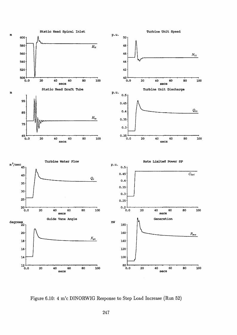
Static Head Spiral Inlet600
580 Hu560
540
520
5000.0 20 40 8060 100secs
Static Head Draft Tube
95
85
75
650.0 20 40 60 80 100secs
Turbine Water Flowm3/ sec
4 D
40
35
30
25
200.0 20 40 60 80 100secs
Guide Vane Angledegrees22
20
18
16
14
12 1008020 40 600.0
Turbine Unit Speed50
48
46
44
42
400.0 20 60 8040 100secsTurbine Unit Discharge
0 .5
0.45
0 .4
0.35
0 .3
0.25 1000.0 20 40 60 80secs
Rate Limited Power SP0 .5
Cltrl0 .45
0 .4
0 .35
0 .3
0 .25
0.260 80 1000.0 20 40 secs
Generation180
160
140
120
100
8060 80 1000.0 20 40
Figure 6.10: 4 m ’c DINORWIG Response to Step Load Increase (Run 52)

£ © . (e>.KO
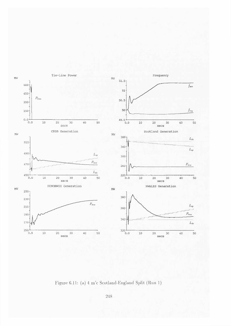
Tie-Line PowerMW
MW
MW
600
450
300
150
0.00.0 10 20 30 40 50
secs CEGB Generation
510
490
470
4500.0 10 20 30 40 50secs
DINORWIG Generation250
230
210
190
170
1500.0 10 20 30 40 50
HZFrequency
MW
MW
51.5
51
5 0 .5
ccg
4 9 .50.0 20 3010 40 50
secsScotland Generation
380
340
300
260
2200.0 3010 20 40 50secs
NWALES Generation
380
360
340
3200.0 10 20 30 40 50
Figure 6.11: (a) 4 m ’c Scotland-England Split (Run 1)
248

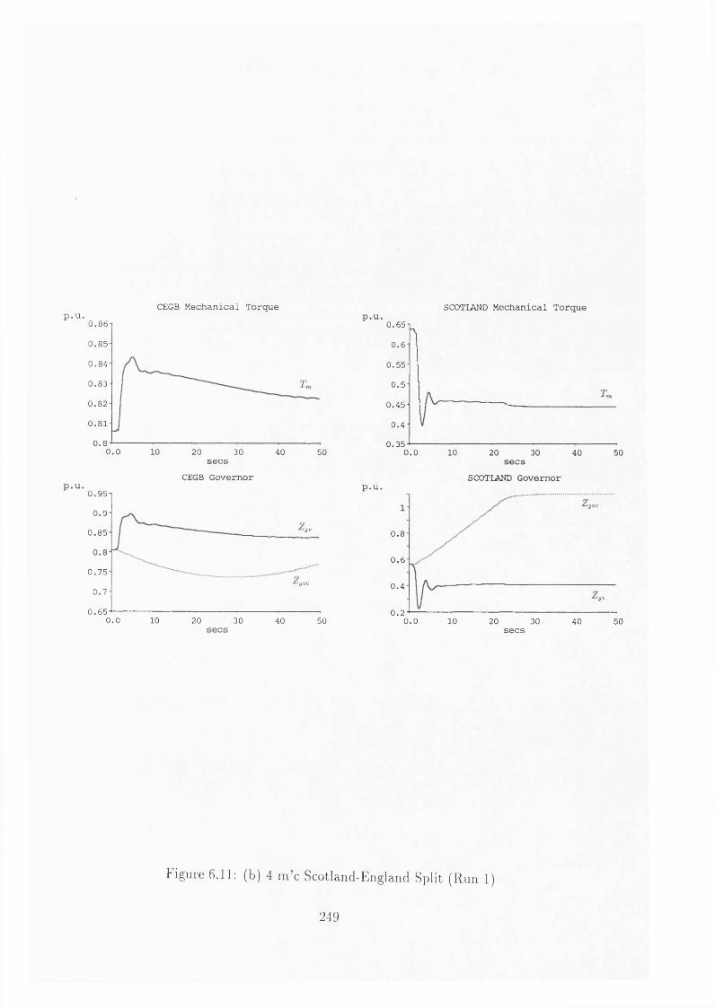
CEGB Mechanical Torquep.u. U.Bb0 .8 5
0 .8 4
0 .8 3
0 .8 2
0 .8 1
0.80 . 0 10 20 30 40 50secs
CEGB Governor0.95-1
0 .9
Igv0 .8 5
0 .7 5 -igtlC
0 .7 -
0 .6 50 . 0 10 20 30 40 50
SCOTLAND Mechanical Torque0.65
0 . 6
0 .5 5
0 .5
0 .4 5
0 .4
0 .3 50.0 10 20 30 40 50secs
SCOTLAND Governorp.u.
'JV C
0.8
0.6
0 .4'J V
0 . 20.0 10 20 30 40 50secs
Figure 6.11: (b) 4 m ’c Scotland-England Split (Run 1)
249

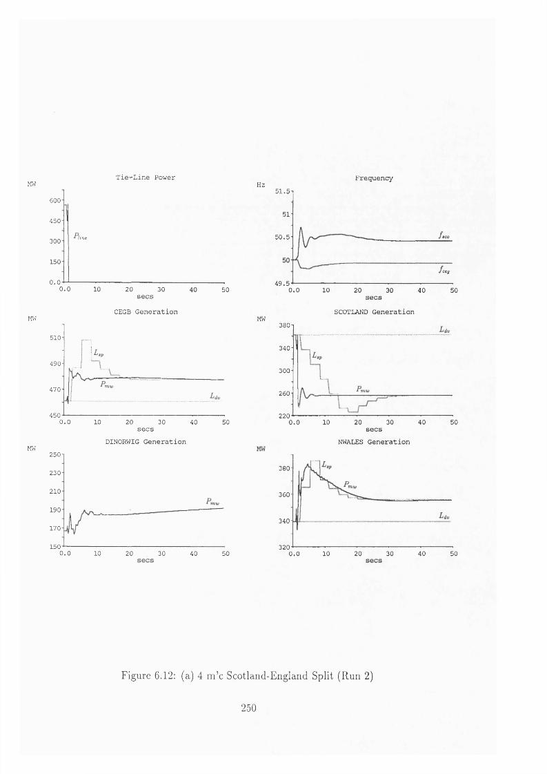
Tie-Line PowerMW
600
450
line300
150
0.00.0 10 20 30 50secs CEGB GenerationMW
510
490
470
4500.0 10 20 30 40 50secs
DINORWIG GenerationMW250
230
210
190
170
1500.0 10 20 30 5040
FrequencyHz 51.5
51
5 0 .5
'ceg
4 9 .5 100.0 20 30 40 50secs
SCOTLAND GenerationMW
380
340
300
260
220 10 20 30 40 500.0secs
NWALES Generation
380
360
340
3200.0 10 20 30 40 50
Figure 6.12: (a) 4 m ’c Scotland-England Split (Run 2)
250
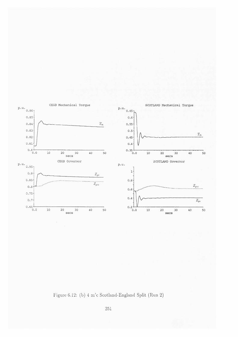
CEGB Mechanical Torque0.860 .8 5
0 .8 4
0 .8 3
0 .8 2
0 .8 1
0.80.0 10 20 30 40 50secs CEGB Governor
0 .9 5
0 .9 'gv
0 .8 5'JV C8
0 .7 5
0 .7
0 .6 50.0 10 20 30 40 50
SCOTLAND Mechanical Torque0.650.6
0 .5 5
0 .5
0 .4 5
0 .4
0 .3 50.0 10 20 30 40 50secsSCOTLAND Governor
p.u.
0.8'J V C
0.6
0 .4' jv
0.20.0 10 20 30 40 50
Figure 6.12: (b) 4 m ’c Scotland-England Split (Run 2)
251
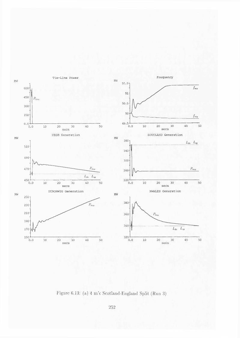
Tie-Line Power FrequencyMW
600
450line
300
150
0.030 40 50200.0 10
secsCEGB Generation
510-
490-
470-
450500.0 10 20 30 40
secsDINORWIG GenerationMW
250
230
210
190
170
1500.0 10 20 30 40 50secs
Hz 51.5
5 0 .5
50ceg
4 9 .540 5020 30100.0 secs
SCOTLAND Generation380
340
300
260
22040 500 . 0 10 20 30
secsNWALES Generation
380
360
340<ap
320 10 20 30 40 500.0 secs
Figure 6.13: (a) 4 m ’c Scotland-England Split (Run 3)
252

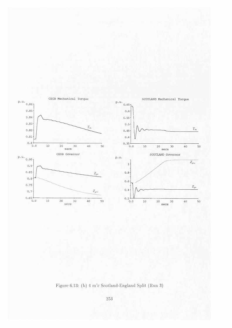
CEGB Mechanical Torque0.860 .8 5 -
0 .8 4 -
0 .8 3 -
0 .8 2 -
0 .8 1
0.80.0 10 20 30 40 50secs
CEGB Governorp.u. u.yo0 .9
0 .8 5
80 .7 5
0 .7 tgvc
0 .6 50.0 10 20 30 40 50secs
SCOTLAND Mechanical Torquep.u. u.to
0.6-0 .5 5
0 .5
0 .4 5 -
0 .4
0 .3 50 . 0 10 20 30 40 50secs
SCOTLAND Governorp.u.'gvc
0 . 6
0 .4
0 . 20 . 0 10 20 30 40 50
Figure 6.13: (b) 4 m ’c Scotland-England Split (Run 3)
253

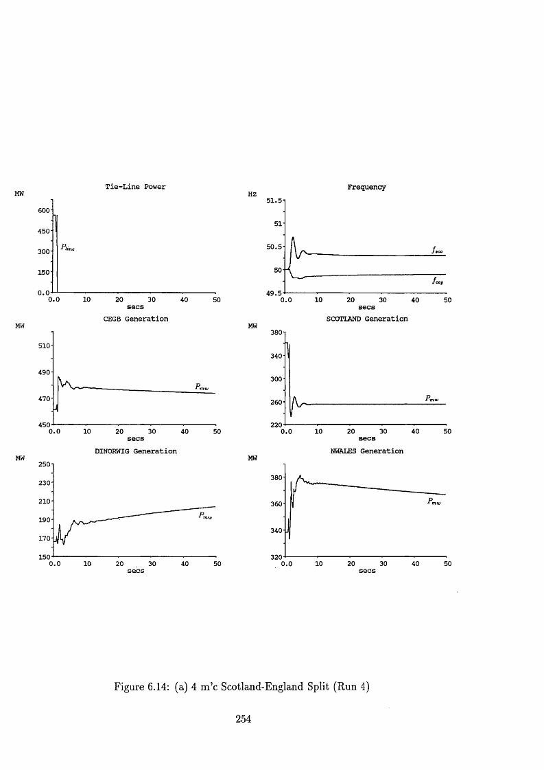
Tie-Line PowerMW
MW
MW
600
450
300
150
0.00.0 10 20 30 40 50secs CEGB Generation
510
490
470
4500.0 10 3020 40 50secsDINORWIG Generation
250
230
210
190
170
1500.0 10 3020 40 50
HZ Frequency51.5i
51
50 .5
50ceg
4 9 .5 100.0 20 30 40 50secsSCOTLAND GenerationMW
380
340
300
260
220 20 30 4010 500.0 secsNWALES GenerationMW
380
360
340
320 10 20 30 40 500.0
Figure 6.14: (a) 4 m ’c Scotland-England Split (Run 4)
254

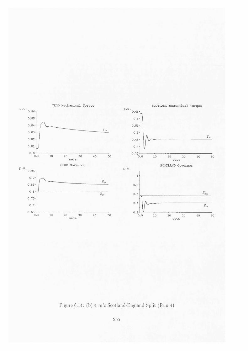
CEGB Mechanical Torquep.u. U.bb
0 .8 5
0 .8 4
0 .8 3
0 .8 2
0 .8 1
0.0 10 20 30 40 50secs
CEGB Governor0.95-1
0 .9 -
0 .8 5 -
0.8igvc
0 .7 5 -
0 .7 -
0 .6 50.0 10 20 30 40 50
SCOTLAND Mechanical Torquep.u. u.tb-i0.6
0 .5 5
0 .5
0 .4 5
0 .4
0 .3 50.0 10 20 30 40 50
secsSCOTLAND Governorp.u.
0.8
0.6
0 .4'gv
0.20.0 10 20 30 40 50secs
Figure 6.14: (b) 4 m ’c Scotland-England Split (Run 4)
255

o WU-t-CcO
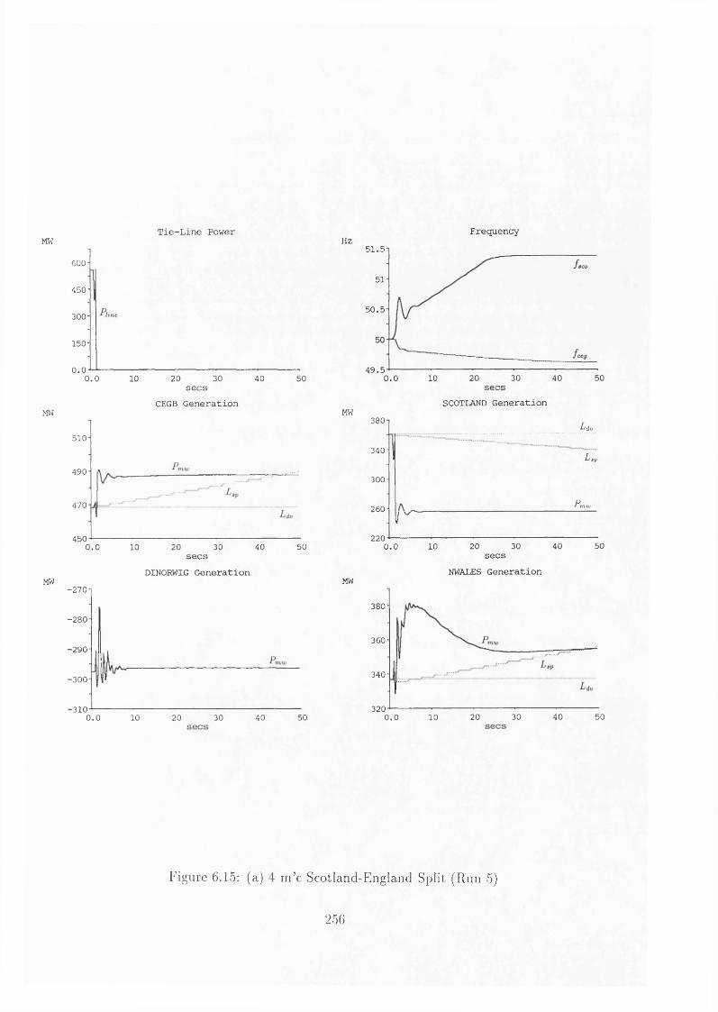
Tie-Line Power FrequencyMW Hz
MW
600
450
300
150
0.00.0 10 20 30 40 50secs
CEGB Generation
secsDINORWIG Generation
MW
510
490
470
45040 500.0 10 20 30
-2 7 0
-2 8 0
-2 9 0
-3 0 0
•310 20 30 40 500.0 10
51.5
51
5 0 .5
4 9 .5 10 20 30 40 500.0secs
SCOTLAND GenerationMW
380
340
300
260
220
L d v
l \ -
L ,p
P m w
r
0.0 10 20 30 40secs
NWALES Generation
50
MW
380
360
340
32030 40 500.0 10 20
Figure 6.15: (a) 4 m ’c Scotland-England Split (Run 5)
256

^ ‘ (a.
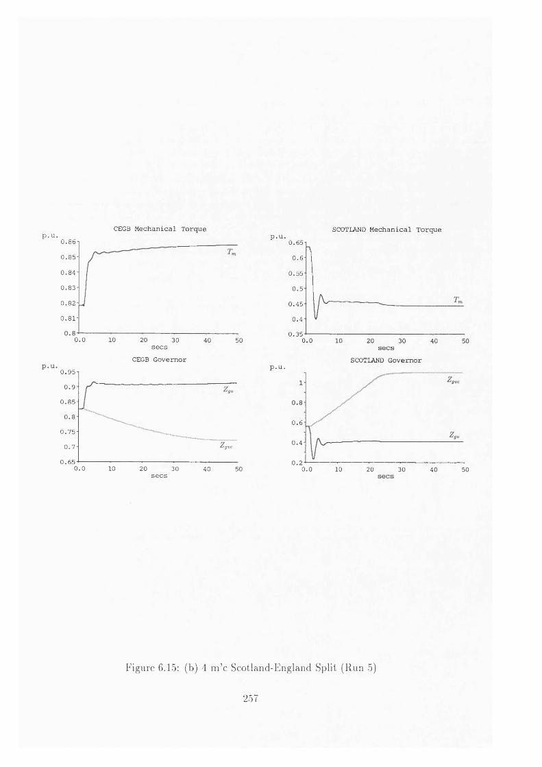
CEGB Mechanical Torquep.u. u.a&i0 .8 5 -
0 .8 4 -
0 .8 3 -
0 .8 2 -
0 .8 1 -
0.0 10 20 30 40 50secs CEGB Governor
0 .9 5
0 .9
0 .8 5
0.80 .7 5
0 .7 'gvc
0 .6 50.0 10 20 30 40 50secs
SCOTLAND Mechanical Torquep.u. U.bS-i0.6-
0 .5 5
0 .5
0 .4 5
0 .4
0 .3 50.0 10 20 30 40 50secs
SCOTLAND Governorp.u.
0.6
0 .4
0.20.0 10 20 30 5040
Figure 6.15: (b) 4 m ’c Scotland-England Split (Run 5)
257

V : I© . \ ^ C & )
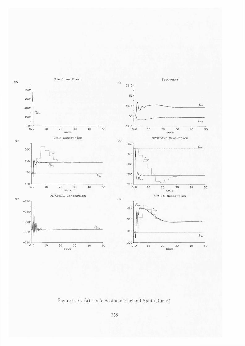
Tie-Line PowerMW
600
450
300
150
0 . 00 . 0 10 20 30 40 50secs
CEGB GenerationMW
510
490
470
4500 . 0 10 20 30 40 50secs
DINORWIG GenerationMW■270
-2 8 0
-2 9 0
•300
•3100.0 10 20 30 40 50
HZFrequency
51.5-1
51
5 0 .5 -
ceg
4 9 .50.0 10 20 30 40 50secs
SCOTLAND GenerationMW380
340
300
260
2200.0 10 20 30 40 50
secsNWALES GenerationMW
380 i L;
360
340
3200.0 10 20 30 40 50
Figure 6.16: (a) 4 m ’c Scotland-England Split (Run 6)
258

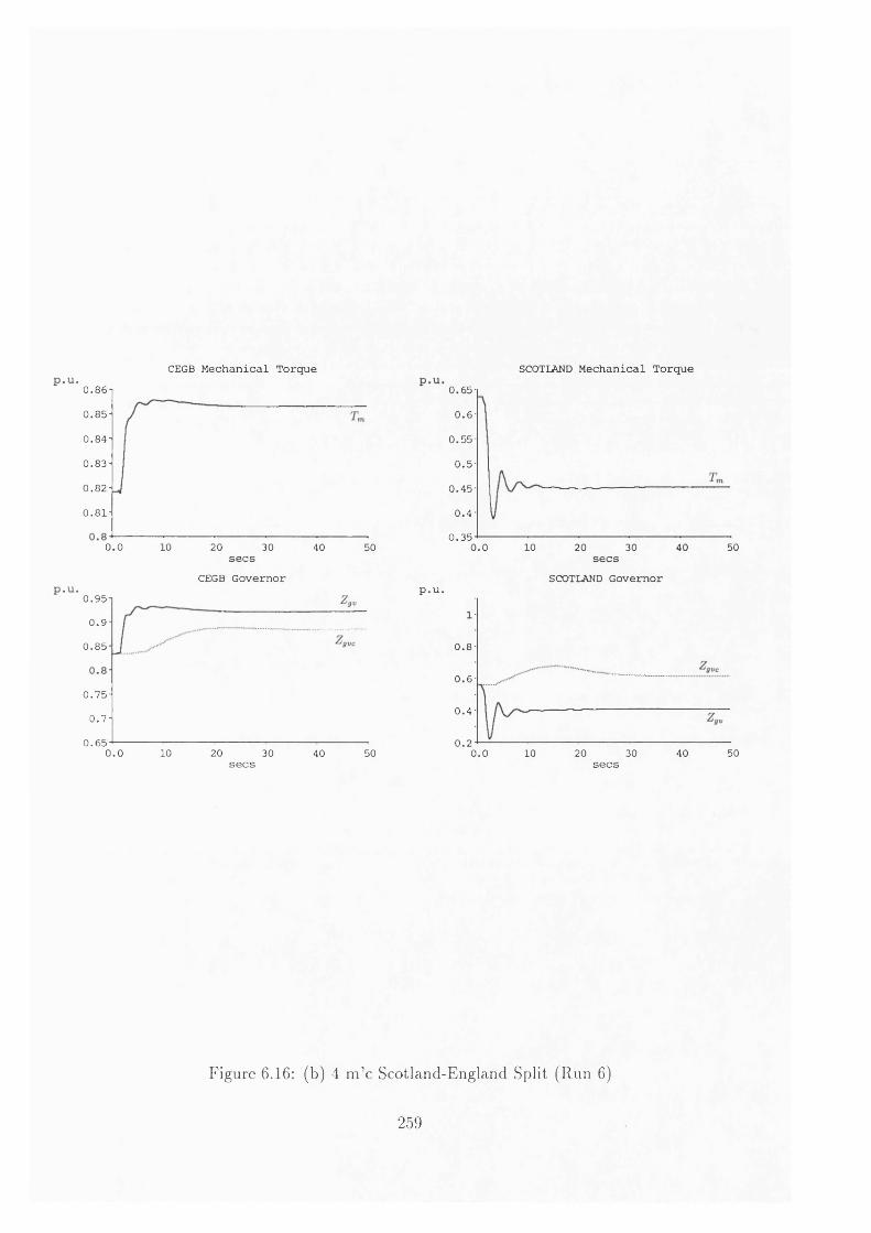
CEGB Mechanical Torque0 .8 6 i
0 .8 5 -
0 .8 4 -
0 .8 3 -
0 .8 2 -
0 .8 1 -
0.0 10 20 30 40 50secs
CEGB Governor0 .9 5 1
0 .9 -
0 .8 5 -
0 .7 5 -
0 .7 -
0 .6 50.0 10 20 30 40 50secs
SCOTLAND Mechanical Torque0.65
0 . 6
0 .5 5
0 .5
0 .4 5
0 .4
0 .3 540 500.0 10 20 30
secsSCOTLAND Governor
p.u.
0.8
0.6
0 .4
0 . 2500.0 10 20 30 40
secs
Figure 6.16: (b) 4 m ’c Scotland-England Split (Run 6)
259

t . i f c O O
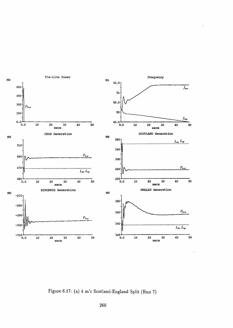
Tie-Line PowerMW
600
450
300line
150
0.00.0 10 20 30 40 50secs
CEGB GenerationMW
510
490
470
45040 5020 300 . 0 10
secsDINORWIG GenerationMW
-270
-280
-290
-300
-3105020 30 400 .0 10
HZFrequency
51.5
51
50 .5
ceg4 9 .5
0 .0 10 20 30 40 50secsSCOTLAND Generation
MW380
340
300
260
220
Ldv L,
0 .0 10 20 30 40 50secs NWALES Generation
MW
380
360
340
3205030 4010 200.0
Figure 6.17: (a) 4 m ’c Scotland-England Split (Run 7)
260

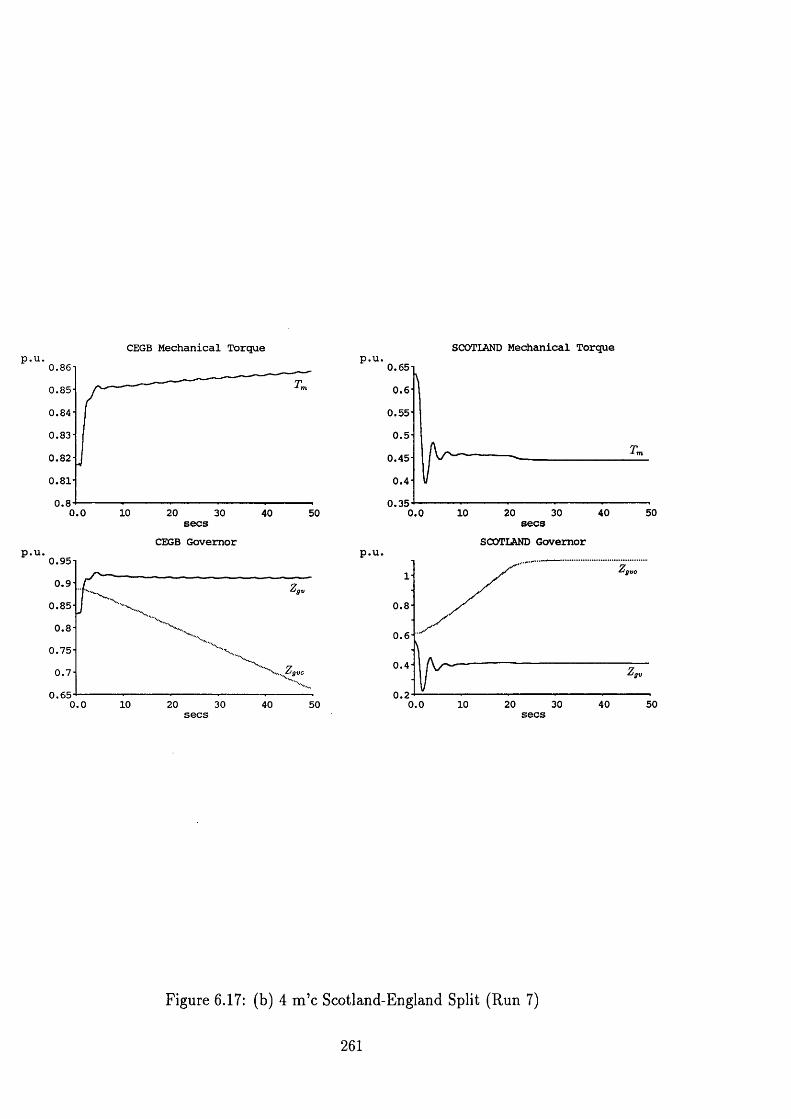
CEGB Mechanical Torque0.86-10 .85-
0 .84-
0 .83-
0 .82-
0 .81 -
0.80.0 10 20 30 40 50secsCEGB Governor
0.95-1
0 .9 -
0 .85-
0.8-0 .75-
0 .7 -
0 .6 50.0 10 20 30 40 50
SCOTLAND Mechanical Torque0.650.6
0 .55
0 .5
0 .45
0 .4
0 .35 20 30 40 500.0 10 secs SCOTLAND Governor
p.u.
0.8
0.6
0 .4
0.2 20 30 40 500.0 10
Figure 6.17: (b) 4 m ’c Scotland-England Split (Run 7)
261

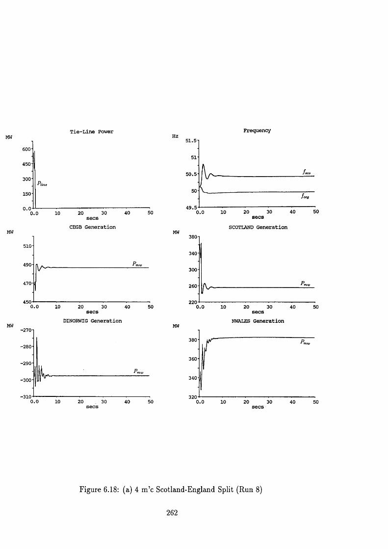
Tie-Line Power FrequencyMW
600
450
300
150
0.050403020100.0 secs
CEGB GenerationMW
510
490
470
4500.0 10 20 30 40 50secsDINORWIG GenerationMW
-270
-280
-290
-300
-3100.0 10 20 30 40 50
Hz 51.5-
51-
50.5-
50-
4 9 .5504030200.0 secs
SCOTLAND GenerationMW380
340
300
260
2200.0 10 20 30 40 50secsNWALES GenerationMW
380
360
340
3200.0 10 20 30 40 50
Figure 6.18: (a) 4 m ’c Scotland-England Split (Run 8)
262

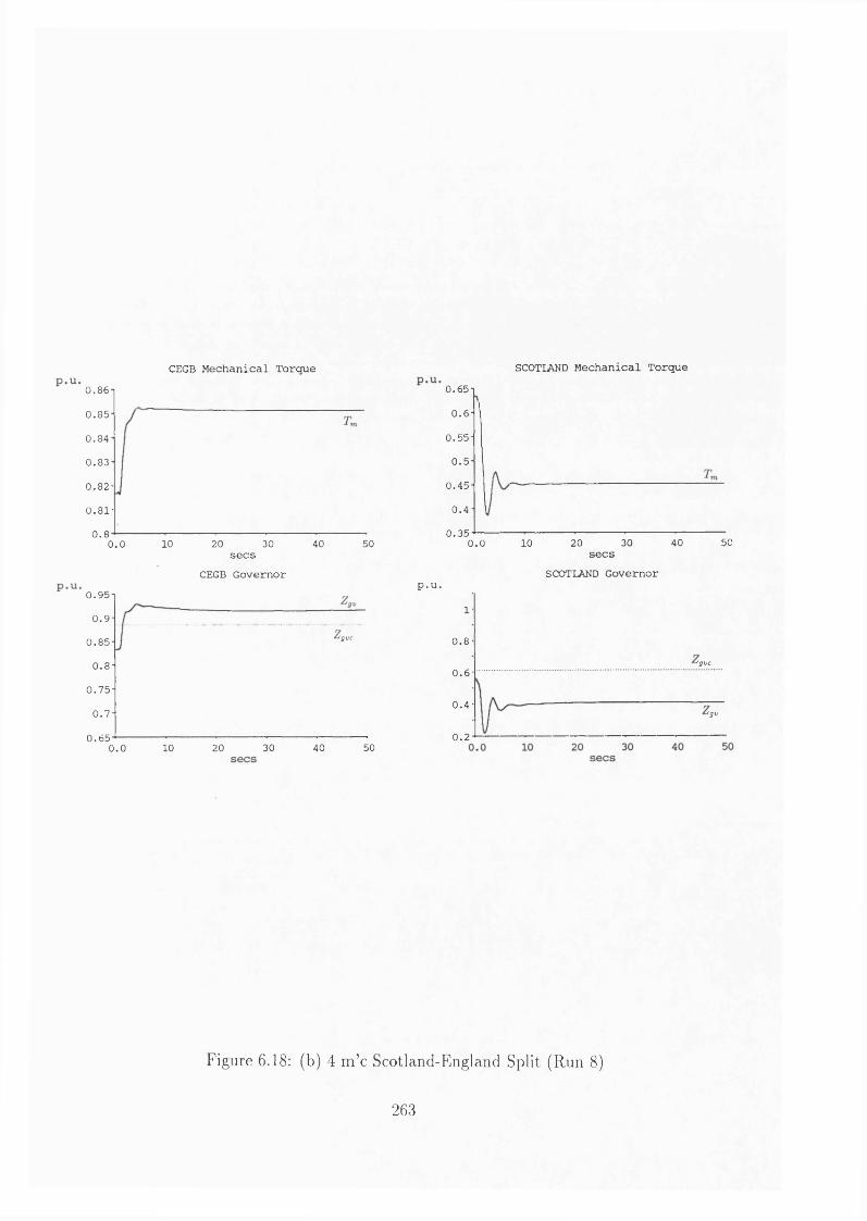
CEGB Mechanical TorqueO.86-1
0 .8 5
0 .8 4
0 .8 3
0 .8 2 -
0 .8 1 -
0.8 10 20 30 40 500.0secs
CEGB Governor0 .9 5
0 .9
Igvc0 .8 5
0.80 .7 5
0 .7
0 .6 5500.0 10 20 30 40
SCOTLAND Mechanical Torque0.650.6
0 .5 5
0 .5
0 .4 5
0 .4
0 .3 55020 30 400.0 10 secs
SCOTLAND Governorp.u.
1
0.8'gvc
0.6
0 .4'gv
0.2
Figure 6.18: (b) 4 m ’c Scotland-England Split (Run 8)
263

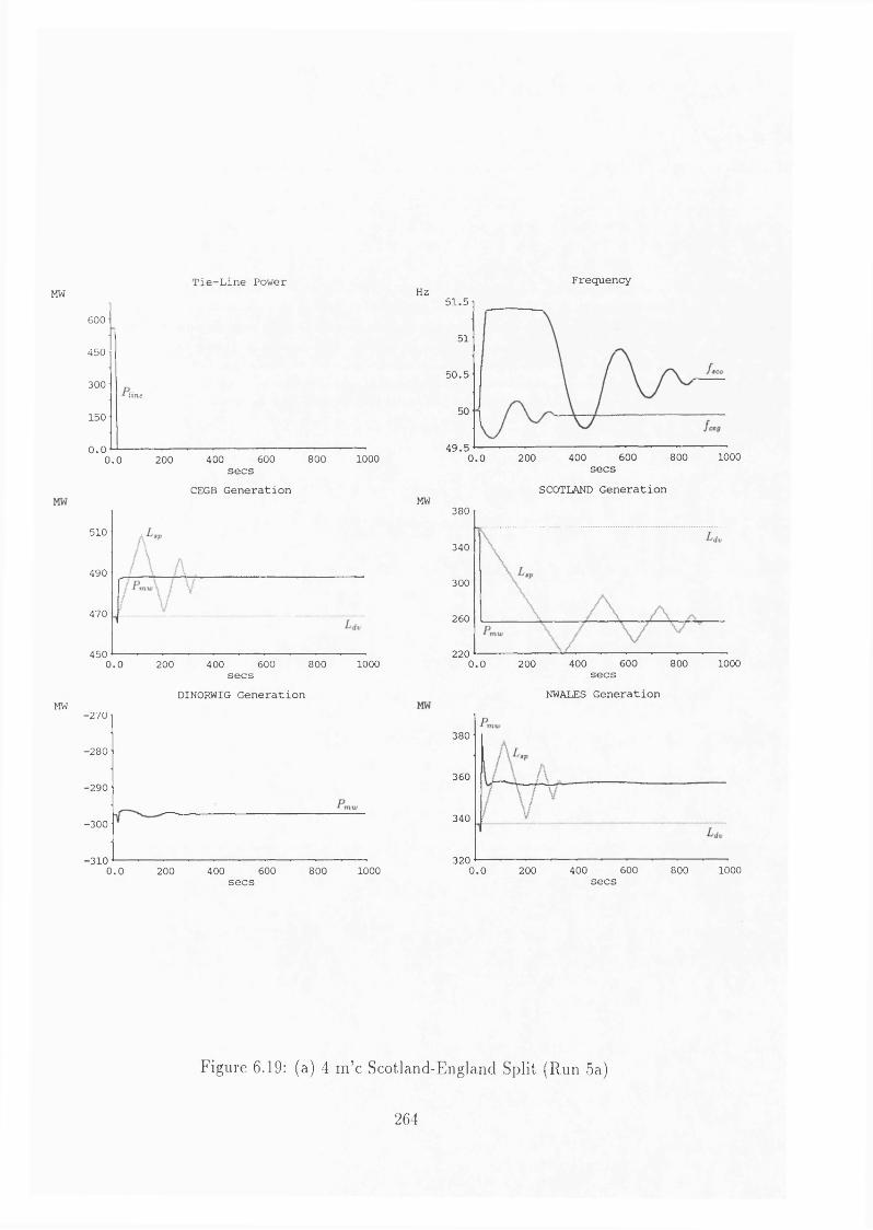
Tie-Line Power FrequencyMW
600
450
300line
150
0.01000600 800200 4000.0
secsCEGB Generation
510
490
470
4500 .0 200 400 600 800 1000
secsDINORWIG Generation
MW-2 7 0
-2 8 0
-2 9 0
-3 0 0
■31010000.0 200 400 600 800
secs
Hz 51.5
51
5 0 .5
50
4 9 .51000600 800200 4000.0 secs
SCOTLAND GenerationMW
380
340
300
260
220400 600 800 10000.0 200 secs
NWALES Generation
380
360
340
320400 600 800 10000.0 200
secs
Figure 6.19: (a) 4 m ’c Scotland-England Split (Run 5a)
264

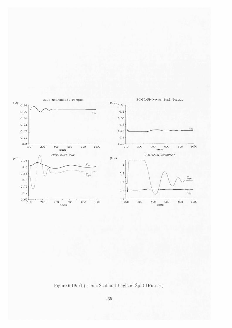
CEGB Mechanical Torque SCOTLAND Mechanical Torquep.u.
0 .8 5
0 .8 4
0 .8 3
0 .8 2
0 .8 1
8400 600 800 10000.0 200
secs CEGB Governor
0 .9 5Igv
0 .9
0 .8 5
0 .7 5
0 .7
0 .6 5600 800 10000.0 200 400
0.650.6
0 .5 5
0 .5
0 .4 5
0 .4
0 .3 510000.0 200 400 600 800
secsSCOTLAND Governor
p.u.
0.8'gvc
0.6
0 .4
0.2 200 400 600 10000.0 800
Figure 6.19: (b) 4 m ’c Scotland-England Split (Run 5a)
265

G to v j
l* U * >
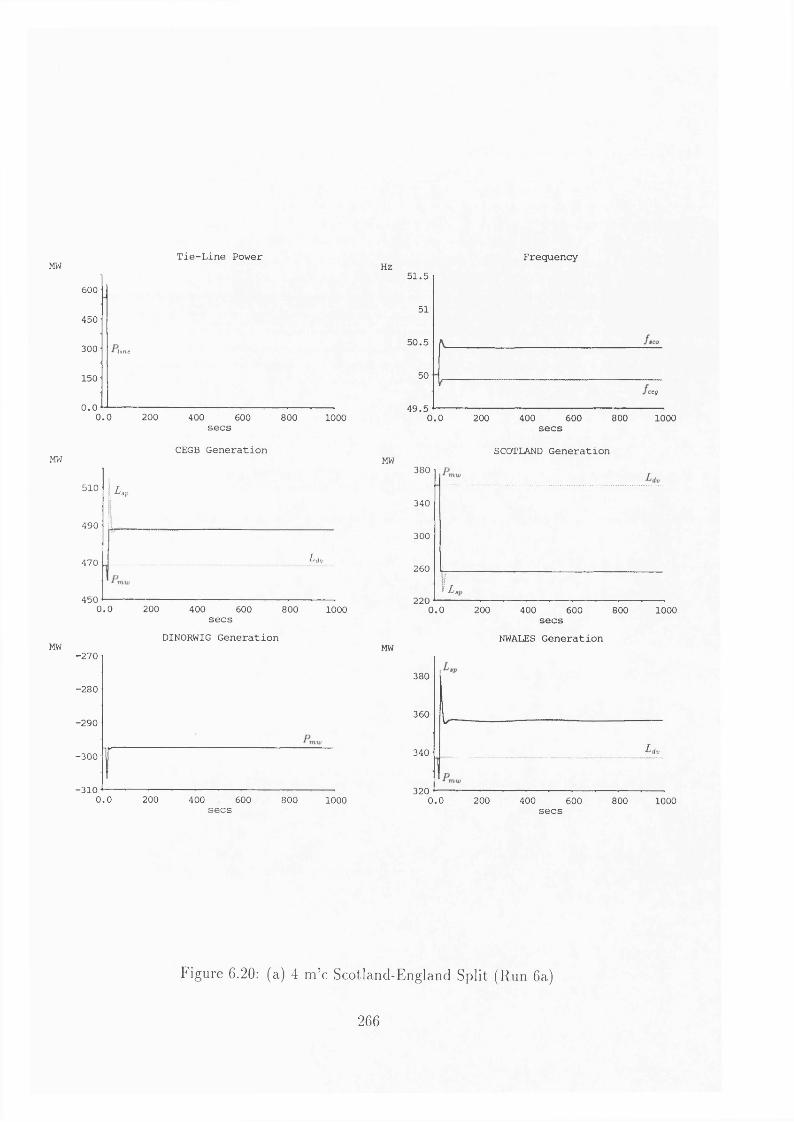
MW Tie-Line Power
MW
MW
600
450
300 line
150
0.00.0 200 400 600 800 1000secs
CEGB Generation
510
490
470
450
\ k
Liv
0.0 200 400 600 800secs
DINORWIG Generation
1000
-2 7 0
-2 8 0
-2 9 0
-3 0 0
-3 1 0r
0 .0 200 400 600secs 800 1000
Hz Frequency
MW
MW
51.5
51
5 0 .5
50ceg
4 9 .50.0 200 400 600 800 1000secs
SCOTLAND Generation380
340
300
260
220■iU.
0 .0 200 400 600 800 1000secs
NWALES Generation
380
360
340
320
ILdv
0 .0 200 400 600 800 1000secs
Figure 6.20: (a) 4 m ’c Scotland-England Split (Run 6a)
266

f c a - f r ^ k . ' x o O o ' )
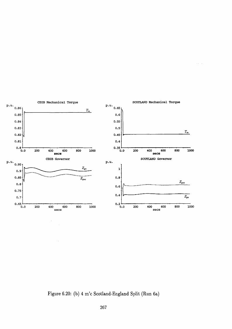
CEGB Mechanical Torque0.860 .8 5
0 .8 4
0 .83
0 .8 2
0 .8 1
0.8 200 400 8000.0 600 1000secs CEGB Governor
0 .9 5
0 .9
0 .8 5
0.80 .7 5
0 .7
0 .6 50.0 200 400 600 800 1000
SCOTLAND Mechanical Torque0.650.6
0.55
0 .5
0 .45
0 .4
0.35600 800 10004002000.0 secs
SCOTLAND Governor p.u.
0.8tgVC
0.6
0 .4
0.2400 600 800 10002000.0
Figure 6.20: (b) 4 m ’c Scotland-England Split (Run 6a)
267

4.P (o ? o WO
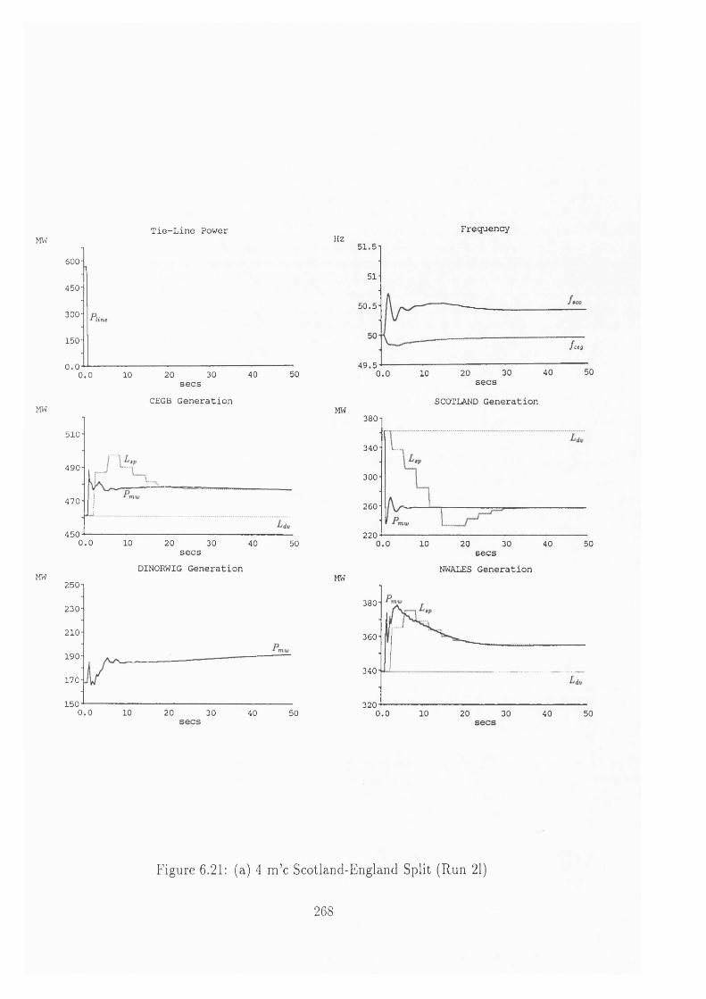
Tie-Line Power FrequencyMW
MW
MW
600
450
300
150
0.040 5020 300.0 10
secs CEGB Generation
510
490
470
4500.0 10 20 30 40 50secs
DINORWIG Generation250
230
210
190
170
1500.0 10 20 30 40 50
Hz 51.5
51
5 0 .5
ccs
4 9 .540 5030200.0 10
MW
MW
secsSCOTLAND Generation
380
340
300
260
2200.0 10 20 5030 40secs
NWALES Generation
380
360
340
3200.0 10 20 30 40 50
Figure 6.21: (a) 4 m ’c Scotland-England Split (Run 21)
268
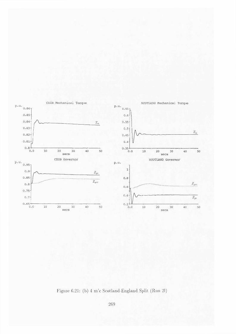
CEGB Mechanical Torquep.u. U.Ot)0 .8 5
0 .8 4
0 .8 3
0 .8 2
0 .8 1
0.80.0 10 20 30 40 50secs
CEGB Governorp.u. u.yo
0 .9
0 .8 5'JV C0.8
0 .7 5
0 .7
0 .6 50.0 10 20 4030 50
SCOTLAND Mechanical Torque0 .6 5
0.60 .5 5
0 .5
0 .4 5
0 .4
0 .3 50.0 2010 30 40 50secs
SCOTLAND Governor p.u.
'gvc0.6
0 .4'J V
0.20.0 10 20 30 40 50secs
Figure 6.21: (b) 4 m ’c Scotland-England Split (Run 21)
269

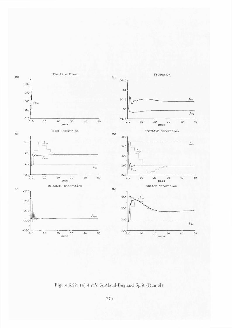
MW Tie-Line Power
600
450
300
150
0.00.0 10 20 30 40 50secs CEGB GenerationMW
secsDINORWIG GenerationMW
510
i__490 ....V.
470
4500.0 10 20 30 40 50
-2 7 0
-2 8 0
■290
-3 0 0
-3 1 00.0 10 20 30 5040
Hz Frequency
MW
MW
51-5
51
5 0 .5
ceg
4 9 .50.0 10 20 30 40 50secs
SCOTLAND Generation380
340
300
260
2200.0 10 20 30 40 50secs
NWALES Generation
380
360
340
3200.0 10 20 30 40 50
Figure 6.22: (a) 4 m ’c Scotland-England Split (Run 61)
270

&
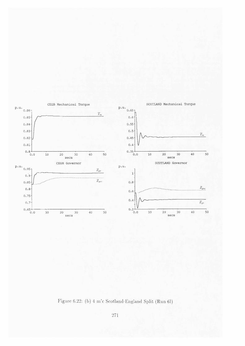
CEGB Mechanical TorqueO.86-1
0 .8 5 -
0 .8 4 -
0 .8 3 -
0 .8 2 -
0 .8 1 -
30 40 500.0 10 20secs
CEGB Governor0 . 95-1
0 .9 -
1 gvc0 .8 5
0 .7 5
0 .7
0 .6 5 20 30 40 500.0 10secs
SCOTLAND Mechanical Torque0.650.6
0 .5 5
0 .5
0 .4 5
0 .4
0 .3 540 5010 20 300.0 secs
SCOTLAND Governorp.u.
1
0.8
0.6
0 .4Igv
0.25020 30 400.0 10 secs
Figure 6.22: (b) 4 m ’c Scotland-England Split (Run 61)
271

<Kr.
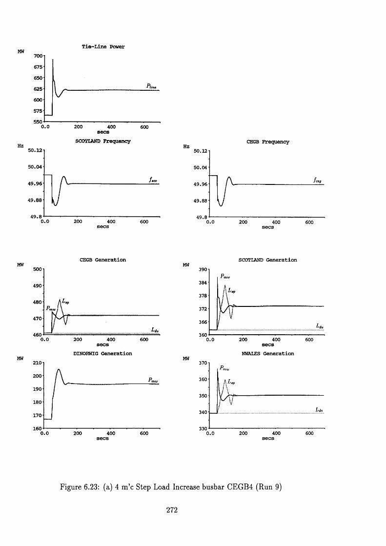
Tie-Line PowerMW 700675
650
625
600
575
5500.0 200 400 600secs
SCOTLAND Frequency Hz50 .12
5 0 .04
4 9 .9 6
4 9 .8 8
4 9 .80.0 200 400 600secs
CEGB Generation MW500
490
480
470
460 2000.0 400 600secs DINORWIG Generation MW 210
200
190
180
170
1600.0 400 600200
CEGB Frequency50.12
50.04
ceg49 .96
49.88
49 .80.0 200 400 600secs
SCOTLAND Generation MW390
384i\L,
378
372
366
3600 .0 200 400 600secs
NWALES GenerationMW370
360 h.L,
350
340
3300 .0 200 400 600
Figure 6.23: (a) 4 m ’c Step Load Increase busbar CEGB4 (Run 9)
272

'" l
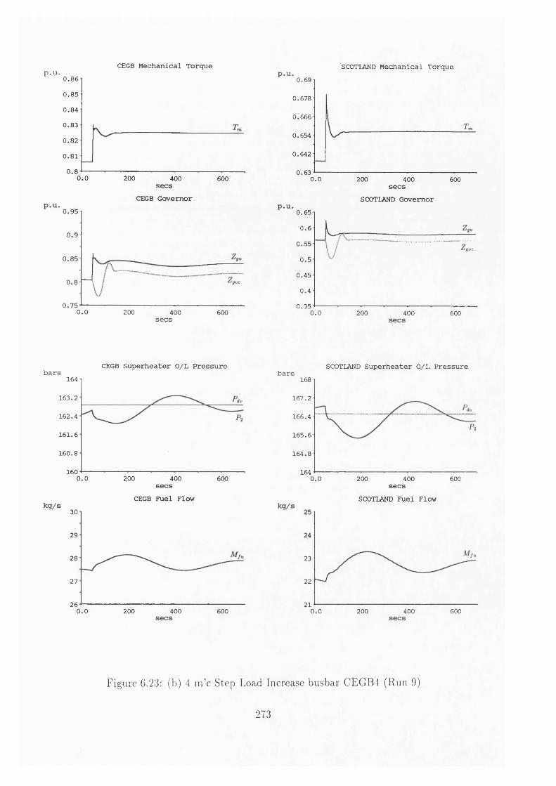
CEGB Mechanical Torquep.u. U.8b
0 .8 5
0 .8 4
0 .8 3
0 .8 2
0 .8 1
0.80.0 200 400 600secs
CEGB Governor0 .9 5
0 .9
0 .8 5
0.8 'gvc
0 .7 50.0 200 400 600secs
SCOTLAND Mechanical Torque0.69
0 .678
0.666
0 .654
0 .642
0 .6 30.0 200 400 600
secsSCOTLAND Governor
0 .6 5
0.60 .5 5
‘gvc
0 .5
0 .4 5
0 .4
0 .3 50.0 200 400 600
CEGB Superheater 0/L Pressurebars164
16 3 .2
16 2 .4
1 6 1 .6
1 6 0 .8
1600.0 200 400 600secs
CEGB Fuel Flow30
29
28
27
260.0 200 400 600
SCOTLAND Superheater 0/L Pressurebars168
1 67 .2
1 66 .4
1 6 5 .6
1 6 4 .8
1640.0 200 400 600secs
SCOTLAND Fuel Flow
23
22
210.0 200 400 600
Figure 6.23: (b) 4 m ’c Step Load Increase busbar CEGB4 (Run 9)
273

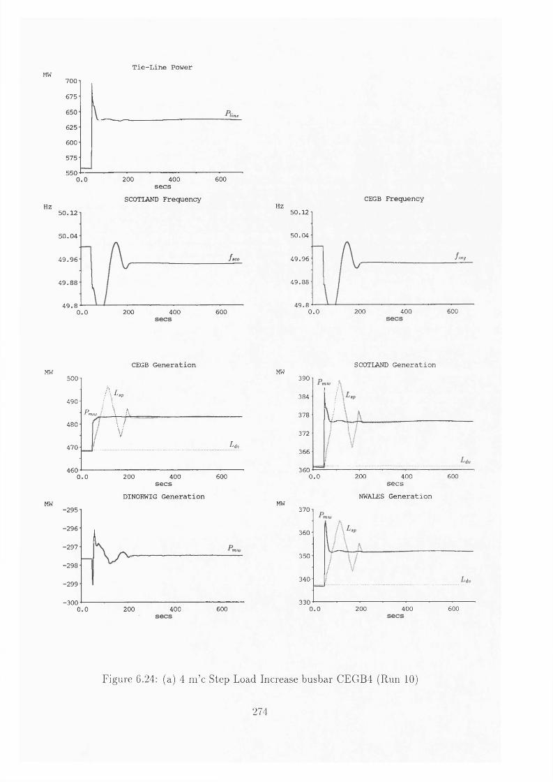
Tie-Line PowerMW 700
675
650 line
625
600
575
5506000.0 200 400
Hz
secsSCOTLAND Frequency
5 0 .1 2
5 0 .0 4
4 9 .9 6
4 9 .8 8
4 9 .8600200 4000.0
HZCEGB Frequency
5 0 .12
50 .04
49 .9 6 ceg
49 .8 8
4 9 .86000.0 200 400
CEGB Generation SCOTLAND GenerationMW
MW
500
490
480
470
460
/wI I P I ' Amu' f » ‘
0.0
\VLdv
200 400secs
600
DINORWIG Generation■295
-2 9 6
-297
■298
-299
-3 0 0 200 400 6000.0
MW
MW
390
384
378
372
366
360 200 400 6000.0secs
NWALES Generation370
360
350
340
330 200 400 6000.0
Figure 6.24: (a) 4 m ’c Step Load Increase busbar CEGB4 (Run 10)
274

i+ L& )
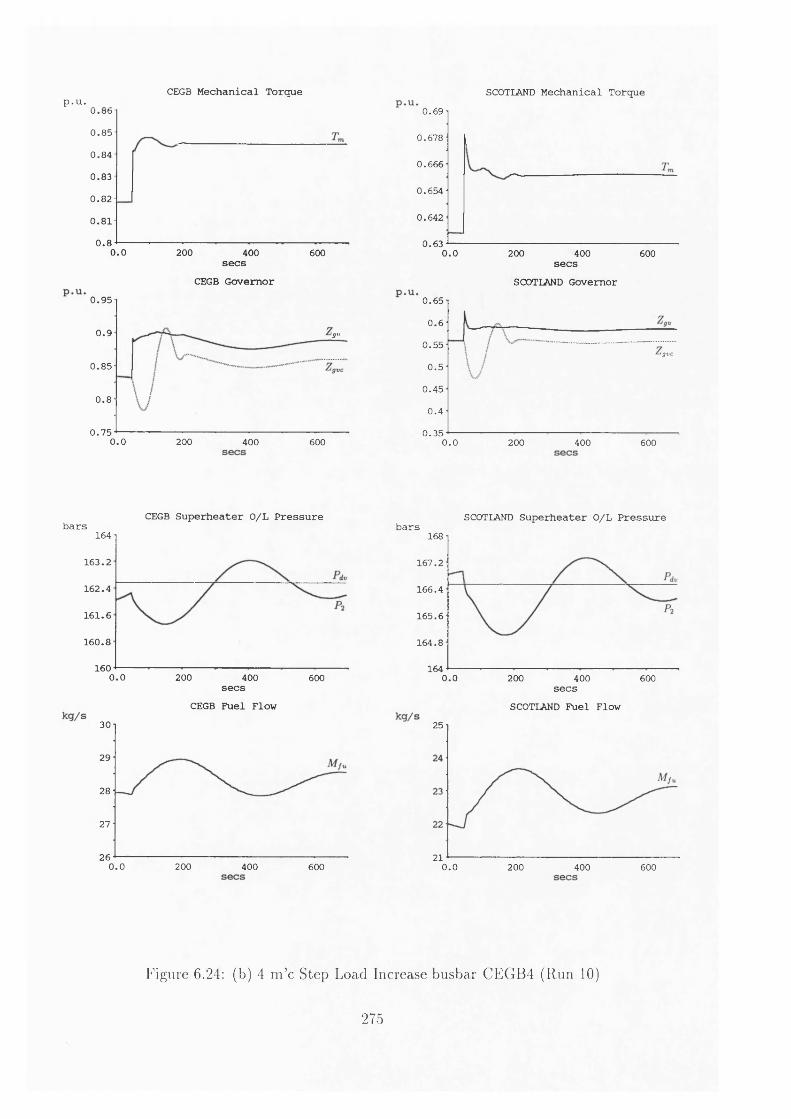
CEGB Mechanical Torquep.u. U.bb0 .8 5
0 .8 4
0 .8 3
0 .8 2
0 .8 1
0 . 80.0 200 400 600
secsCEGB Governor
0 .9 5
0 .9 igv
0 .8 5
0 . 8
0 .7 50.0 200 400 600
SCOTLAND Mechanical Torque0.69
0 .678
0.666
0 .654
0 .642
0 .630.0 200 400 600secs
SCOTLAND Governor0 .6 5
0 . 6
0 .5 5'gvc
0 .5
0 .4 5
0 .4
0 .3 50.0 200 400 600
CEGB Superheater O/L Pressurebars164
1 6 3 .2
1 6 2 .4
1 6 1 .6
1 6 0 .8
1600.0 200 400 600secs
CEGB Fuel Flow30
29
28
27
260.0 200 400 600
SCOTLAND Superheater O/L Pressurebars168
167 .2
166 .4
16 5 .6
164 .8
1640.0 200 400 600
secsSCOTLAND Fuel Flow
25
210.0 200 400 600
Figure 6.24: (b) 4 m ’c Step Load Increase busbar CEGB4 (Run 10)
275

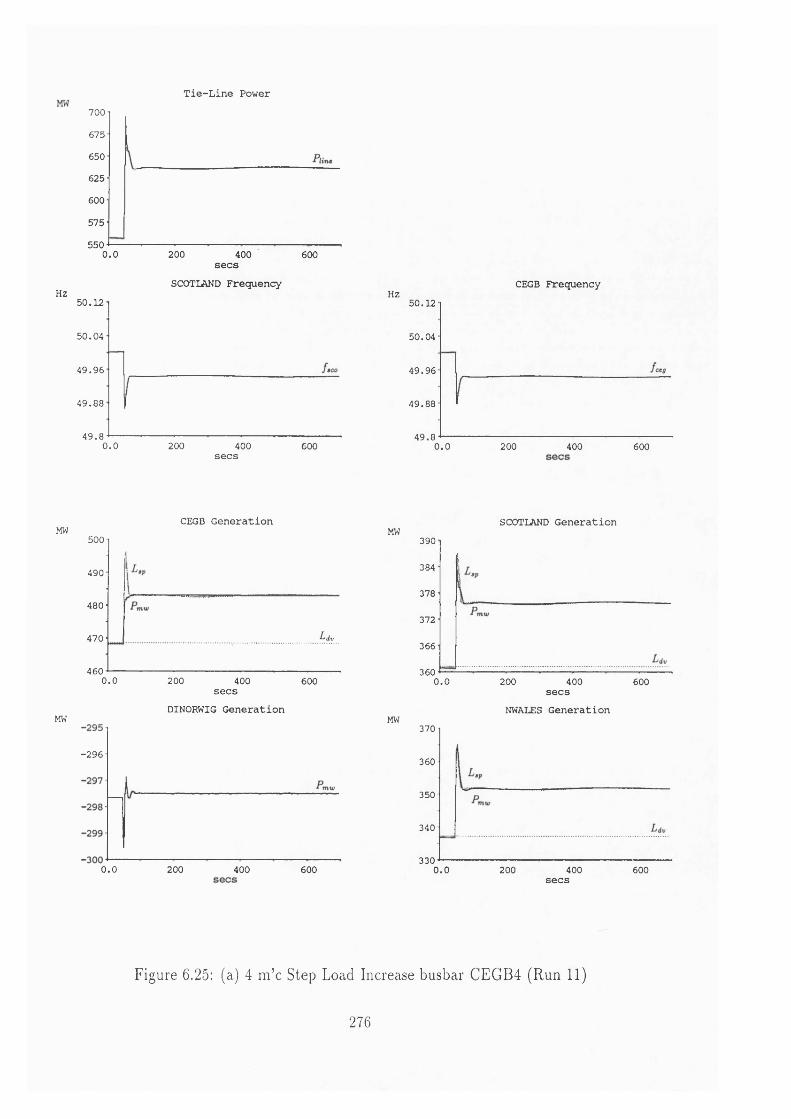
Tie-Line Power700675
650
625
600
575
5500.0 200 400 600
secs SCOTLAND Frequency
Hz50 .1 2
5 0 .0 4
4 9 .9 6
49 .8 8
4 9 .80.0 200 400 600secs
CEGB FrequencyHz
50 .12
50 .04
4 9 .9 6
49 .8 8
4 9 .80.0 200 400 600
MW500
490
480
470
4600.0
MW
CEGB Generation
Ldv
200 400 600secs
DINORWIG Generation
-2 9 6
0.0 200 400 600
SCOTLAND GenerationMW
MW
390
384
378
372
366
3600.0 200 400 600secs
NWALES Generation370
360
350
340
3300.0 200 400 600
secs
Figure 6.25: (a) 4 m ’c Step Load Increase busbar CEGB4 (Run 11)
276
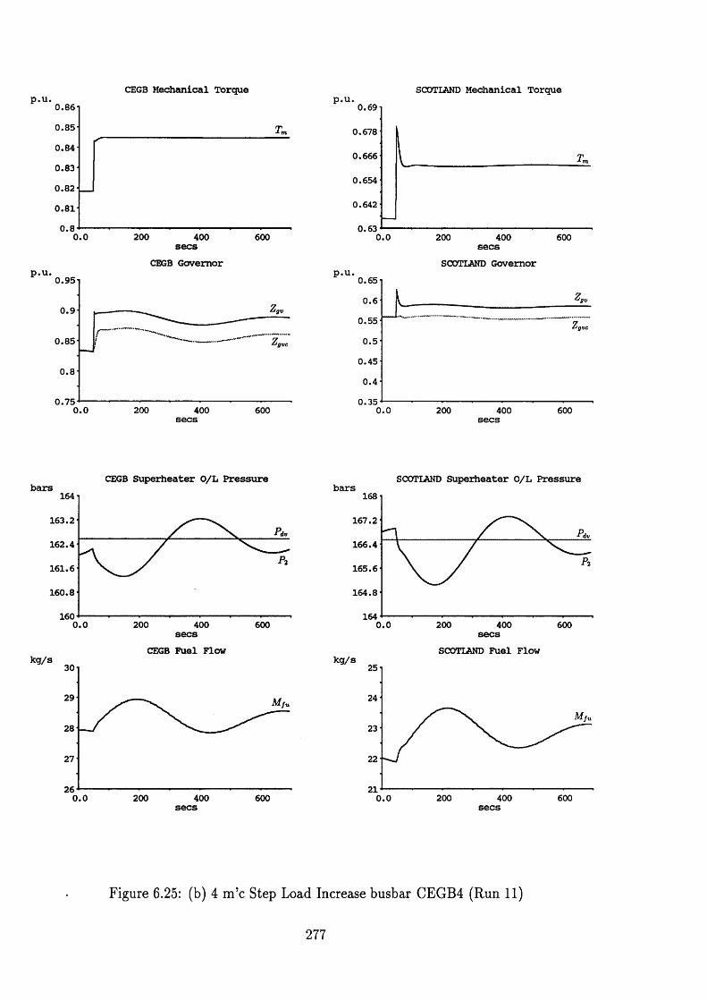
CEGB Mechanical Torque SCOTLAND Mechanical Torque0.860 .8 5
0 .84
0 .8 3
0 .8 2
0 .8 1
0.80.0 200 400 600secs CEGB Governor
0 .9 5
0 .9 tgv
0 .8 5
0.8
0 .7 50.0 200 400 600
0.69
0.678
0 .666
0.654
0.642
0 .630.0 200 400 600secs
SCOTLAND Governor0 .65
0.60 .55
ig tic
0 .5
0 .45
0 .4
0 .350.0 200 400 600
CEGB Superheater O/L Pressure bars164
163.2
162.4
161.6
160.8
160 2000.0 400 600secsCEGB Fuel Flow
30
29
28
27
260.0 200 400 600
SCOTLAND Superheater O/L Pressure bars168
167.2
166.4
165 .6
164.8
1640.0 200 400 600secsSCOTLAND Fuel Flow
21 200 400 6000.0
Figure 6.25: (b) 4 m ’c Step Load Increase busbar CEGB4 (Run 11)
277

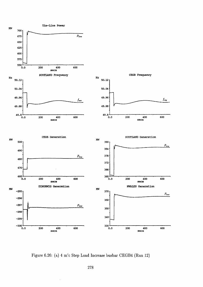
Tie-Line Power700675
650
625
600
575
550400 6000.0 200 secs
SCOTLAND FrequencyHz
50.12
50 .04
4 9 .96
49 .88
4 9 .8600200 4000.0
CEGB FrequencyHz
50.12
50.04
49.96ceg
49.88
4 9 .8400 6002000.0
CEGB GenerationMW500
490
480
470
4600.0 200 400 600
MW
secsDINORWIG Generation
•295
-296
■297
-298
-299
-3000.0 200 400 600
SCOTLAND GenerationMW390
384
378
372
366
360 200 400 6000.0
MW
secsNWALES Generation
370
360
350
340
330 200 400 6000.0 secs
Figure 6.26: (a) 4 m ’c Step Load Increase busbar CEGB4 (Run 12)
278

a jp
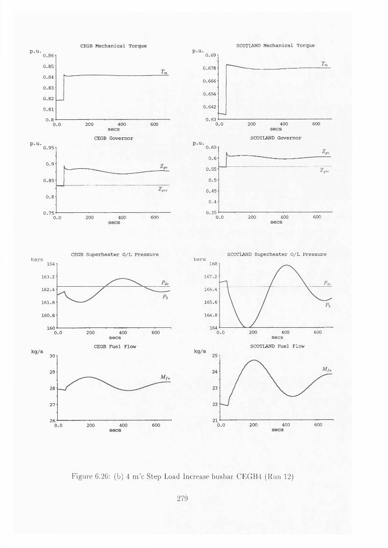
CEGB Mechanical Torque SCOTLAND Mechanical Torque0.860 .8 5
0 .8 4
0 .8 3
0 .8 2
0 .8 1
0.80.0 200 400 600secs
CEGB Governor0 .9 5
0 .9
0 .8 5
'gvc
0.8
0 .7 56000.0 200 400
0.69
0 .6 7 8
0.666
0 .654
0 .642
0 .6 3 200 400 6000.0secs
SCOTLAND Governor0 .6 5
0.60 .5 5 'gvc
0 .5
0 .4 5
0 .4
0 .3 56000.0 200 400
CEGB Superheater O/L Pressure bars
164
1 6 3 .2
1 6 2 .4
1 6 1 .6
1 6 0 .8
1606000.0 200 400
secs CEGB Fuel Flow
30
29
28
27
26 200 400 6000.0
SCOTLAND Superheater O/L Pressure bars
168
167 .2dv
166 .4
1 6 5 .6
164 .8
164 200 400 6000.0secs
SCOTLAND Fuel Flow25
23
22
21 200 400 6000.0
Figure 6.26: (b) 4 m ’c Step Load Increase busbar CEGB4 (Run 12)
279

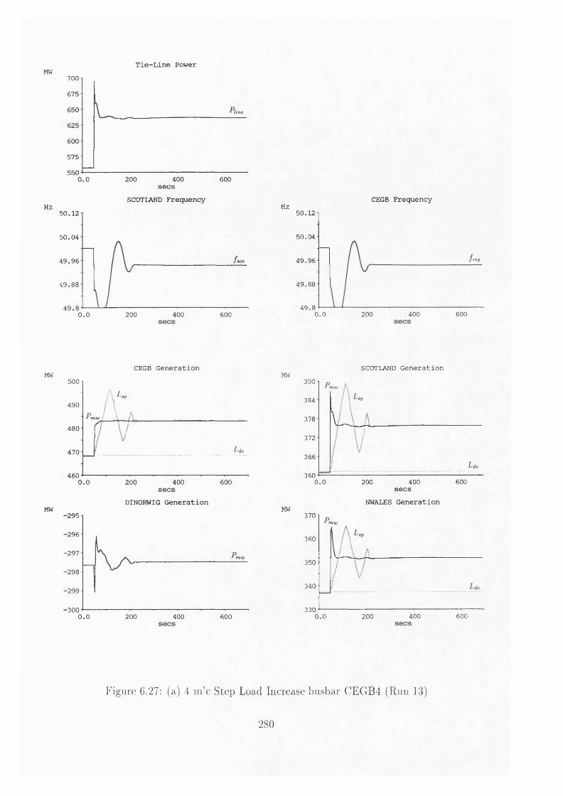
Tie-Line PowerMW 700
675
650 line
625
600
575
550 200 400 6000.0
Hz
secsSCOTLAND Frequency
5 0 .1 2
5 0 .0 4
4 9 .9 6
4 9 .8 8
4 9 .80.0 200 400 600
HZCEGB Frequency
5 0 .1 2
5 0 .0 4
4 9 .9 6 ceg
4 9 .8 8
4 9 .80.0 200 400 600
CEGB Generation SCOTLAND GenerationMW
MW
500
490
480
470
460
A Tj V L»v
p I \ AI \ r
0.0
L d v
200 400secs
600
DINOKWIG Generation•295
-2 9 6
-2 9 7
-2 9 8
-2 9 9
■3000.0 400 600200
MW
MW
390
384
378
372
366
360400 6000.0 200
secsNWALES Generation
370
360
350
340
330400 6000.0 200
Figure 6.27: (a) 4 m ’c Step Load Increase busbar CEGB4 (Run 13)
280

* V i ( c ' j
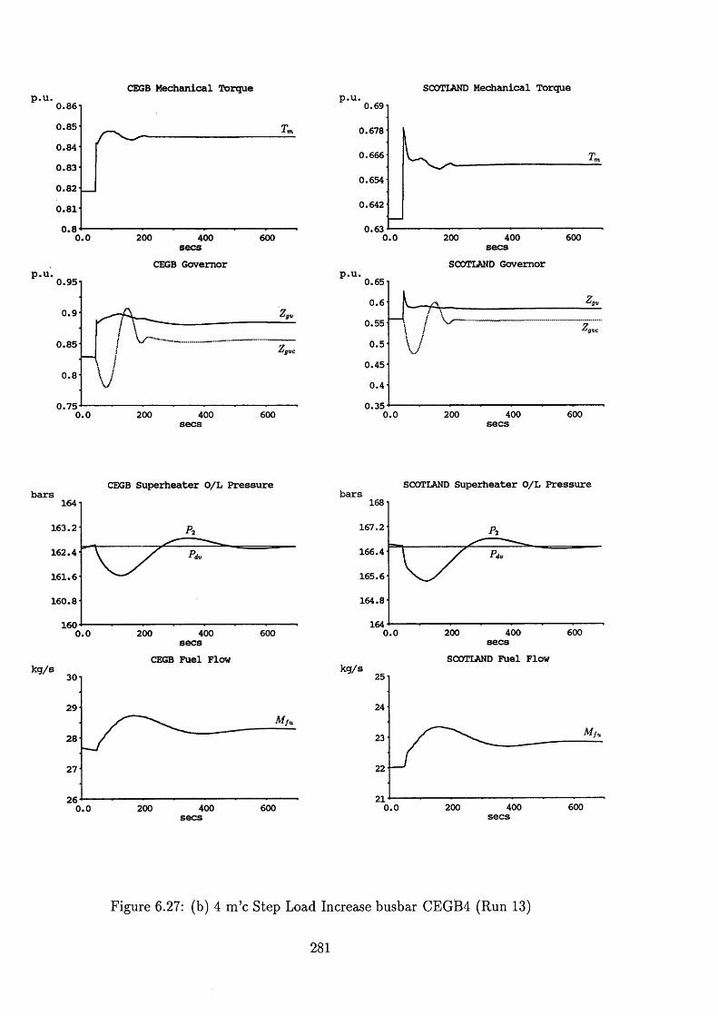
CEGB Mechanical Torque0.860 .8 5
0 .8 4
0 .8 3
0 .8 2
0 .8 1
0.8 2000.0 400 600secs
CEGB Governor0 .9 5
0 .9 'gv
0 .8 5'gvc
0.8
0 .7 50.0 200 400 600
SCOTLAND Mechanical Torque0.69
0.678
0.666
0.654
0.642
0.636004000.0 200
secsSCOTLAND Governor
0 .65
0.60.55
0 .5
0 .45
0 .4
0 .356004000.0 200
CEGB Superheater O/L Pressure bars
164
163 .2
162 .4
1 6 1 .6
160 .8
160400 6000.0 200
secsCEGB Fuel Flow
30
29
28
27
26400 6002000.0
SCOTLAND Superheater O/L Pressurebars
168
167.2
166.4
165.6
164.8
164600200 4000.0 secs
SCOTLAND Fuel Flow25
24
21 6004002000.0
Figure 6.27: (b) 4 m ’c Step Load Increase busbar CEGB4 (Run 13)
281

\o . ' D C C )
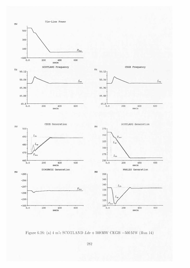
Tie-Line PowerMW
500
300
100
■1000.0 200 400 600secs
SCOTLAND Frequency HZ
5 0 .1 2
5 0 .0 4
4 9 .9 6
4 9 .8 8
4 9 .80.0 400 600200secs
CEGB Generation MW500
490
480
470
4600.0 200 400 600secs
DINOKWIG Generation MW
■295
-2 9 6
■297
•298
-299
■300 200 400 6000.0
CEGB Frequency Hz
5 0 .1 2
5 0 .0 4
4 9 .9 6
4 9 .8 8
4 9 .80.0 200 400 600secs
SCOTLAND Generation MW
375
350
325
300
275
2500 .0 200 400 600
secsNWALES Generation
350
345
340
335
330
325
3200 .0 200 400 600
Figure 6.28: (a) 4 m ’c SCOTLAND Ldv + 500 MW CEGB -500 MW (Run 14)
282

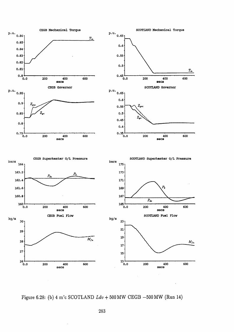
CEGB Mechanical Torque SCOTLAND Mechanical Torque0.860 .8 5
0 .84
0 .83
0 .82
0 .8 1
0.84000.0 200 600
secs CEGB Governor
0 .9 5
0 .9 4gvc
0 .85 fgv
0.8
0 .7 56000.0 200 400secs
0.65
0.6
0 .55
0 .5
0 .4 5400 6000.0 200 secs
SCOTLAND Governor0 .65
0.60 .55 fgv c
0 .5fgv
0 .45
0 .4
0 .35 200 400 6000.0
CEGB Superheater O/L Pressure bars164
163.2
162 .4
1 6 1 .6
160 .8
1600.0 200 400 600secs
CEGB Fuel Flow30
29
28
27
266000.0 200 400
SCOTLAND Superheater O/L Pressure bars175
173
171
169
167
165400 6000.0 200
secsSCOTLAND Fuel Flow
23
21
19
17
15
13400 6002000.0
Figure 6.28: (b) 4 m ’c SCOTLAND L d v + 500 MW CEGB -5 0 0 MW (Run 14)
283
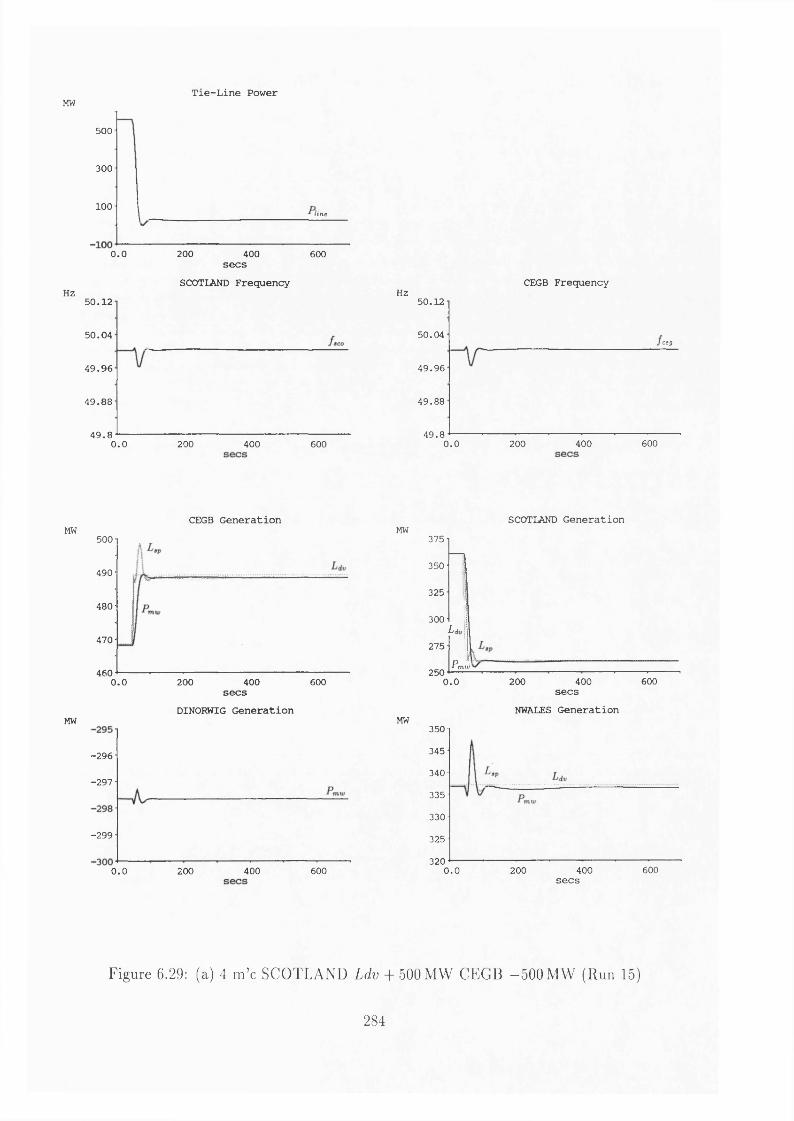
Tie-Line PowerMW
500
300
100line
0.0 200 400 600
Hz
secsSCOTLAND Frequency
5 0 .1 2
5 0 .0 4
4 9 .9 6
4 9 .8 8
4 9 .80.0 200 400 600
HZCEGB Frequency
50.12
50 .04ceg
4 9 .9 6
4 9 .8 8
4 9 .86000.0 200 400
CEGB Generation SCOTLAND GenerationMW
MW
500
490
480
470
4604000.0 200 600
secsDINORWIG Generation
-2 9 6
-2 9 7
-2 9 9
0.0 200 400 600
MW
MW
375
350
325
300
275
250
Li
P m w
0.0 400secs
200
NWALES Generation
600
350
345
340
335
330
325
3206000.0 200 400
secs
Figure 6.29: (a) 4 m ’c SCOTLAND L<fo + 500MW CEGB -500 MW (Run 15)
284

C e \ C o/2O
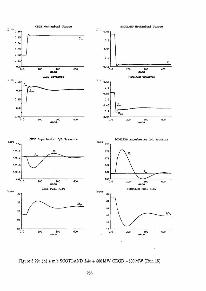
CEGB Mechanical Torque0.860 .8 5
0 .84
0 .83
0 .8 2
0 .8 1
0.80.0 200 400 600secsCEGB Governor
0 .9 5<gv
0 .9 *gvc
0 .8 5
0.8
0 .7 50 .0 400200 600
SCOTLAND Mechanical Torque0.65
0.6
0 .5 5
0 .5
0 .450.0 400200 600secs
SCOTLAND Governor0 .65
0.6
0 .55
0 .5
0 .45
0 .4*gvc
0 .3 50.0 200 400 600
CEGB Superheater O/L Pressurebars164
163.2
162.4
161 .6
160 .8
1600.0 200 400 600secsCEGB Fuel Flow
30
29
28
27
260.0 400200 600
SCOTLAND Superheater O/L Pressurebars175
173
171
169
167
1650.0 200 400 600secs
SCOTLAND Fuel Flow
21
0.0 200 400 600
Figure 6.29: (b) 4 m’c SCOTLAND Ldv + 500 MW CEGB -500 MW (Run 15)
285
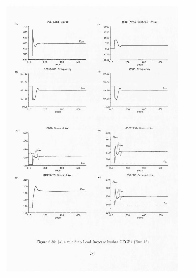
Tie-Line PowerMW
Hz
700675
650
625
600
575
5500.0 200 400 600secs
SCOTLAND Frequency5 0 .1 2
5 0 .0 4
4 9 .9 6
4 9 .8 8
4 9 .86000.0 200 400
CEGB Area Control ErrorMW 3000
2250
1500
750
0.0■750
-1 5 0 0 200 400 6000.0
HZ
secs CEGB Frequency
5 0 .12
5 0 .04
ctg4 9 .9 6
49
4 9 .80.0 200 400 600
CEGB Generation MW
500
490
480P i\x m w f <
470
4600.0 200 400 600secs
DINORWIG Generation MW 210
200
190
180
170
1600 .0 200 400 600
SCOTLAND Generation MW
390
384
378
372
366
3604000.0 200 600
secsNWALES Generation
MW370
360
350
340
3300.0 200 400 600
Figure 6.30: (a) 4 m ’c Step Load Increase busbar CEGB4 (Run 16)
286

( r
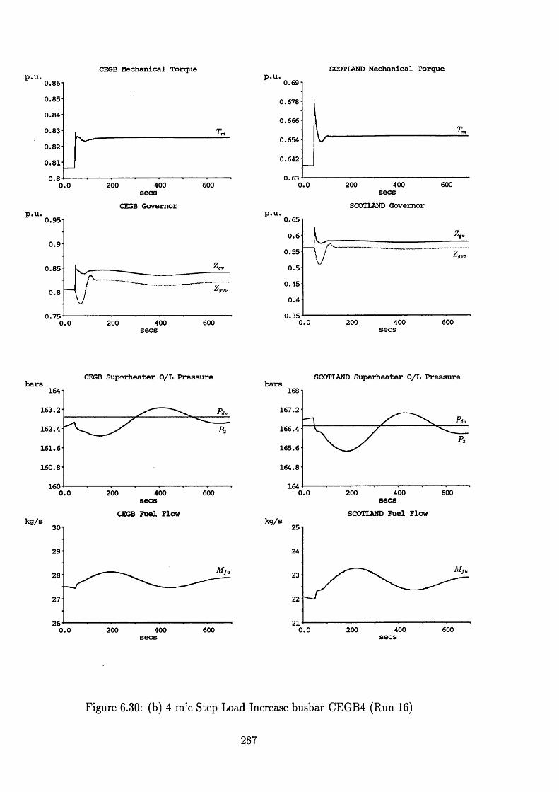
CEGB Mechanical Torque0.860 .8 5
0 .84
0 .83
0 .82
0 .8 1
0.8400 6000.0 200
secs CEGB Governor
0 .9 5
0 .9
0 .8 5
'gvc0.8
0 .7 5400 6002000.0
SCOTLAND Mechanical Torque0.69
0 .678
0 .666
0.654
0.642
0 .63400 6000.0 200 secs
SCOTLAND Governor0 .6 5
0.60 .55 'gvc
0 .5
0 .4 5
0 .4
0 .35600200 4000.0
CEGB Superheater O/L Pressure bars164
163.2
162 .4
161 .6
160 .8
160400 6000.0 200 secs
CEGB Fuel Flow30
29
28
27
266000.0 200 400
SCOTLAND Superheater O/L Pressure bars168
167.2
166.4
165.6
164.8
164400 6002000.0 secs
SCOTLAND Fuel Flow25
21400 6002000.0
Figure 6.30: (b) 4 m ’c Step Load Increase busbar CEGB4 (Run 16)
287

I ip \ O' b ; % o ^ v )
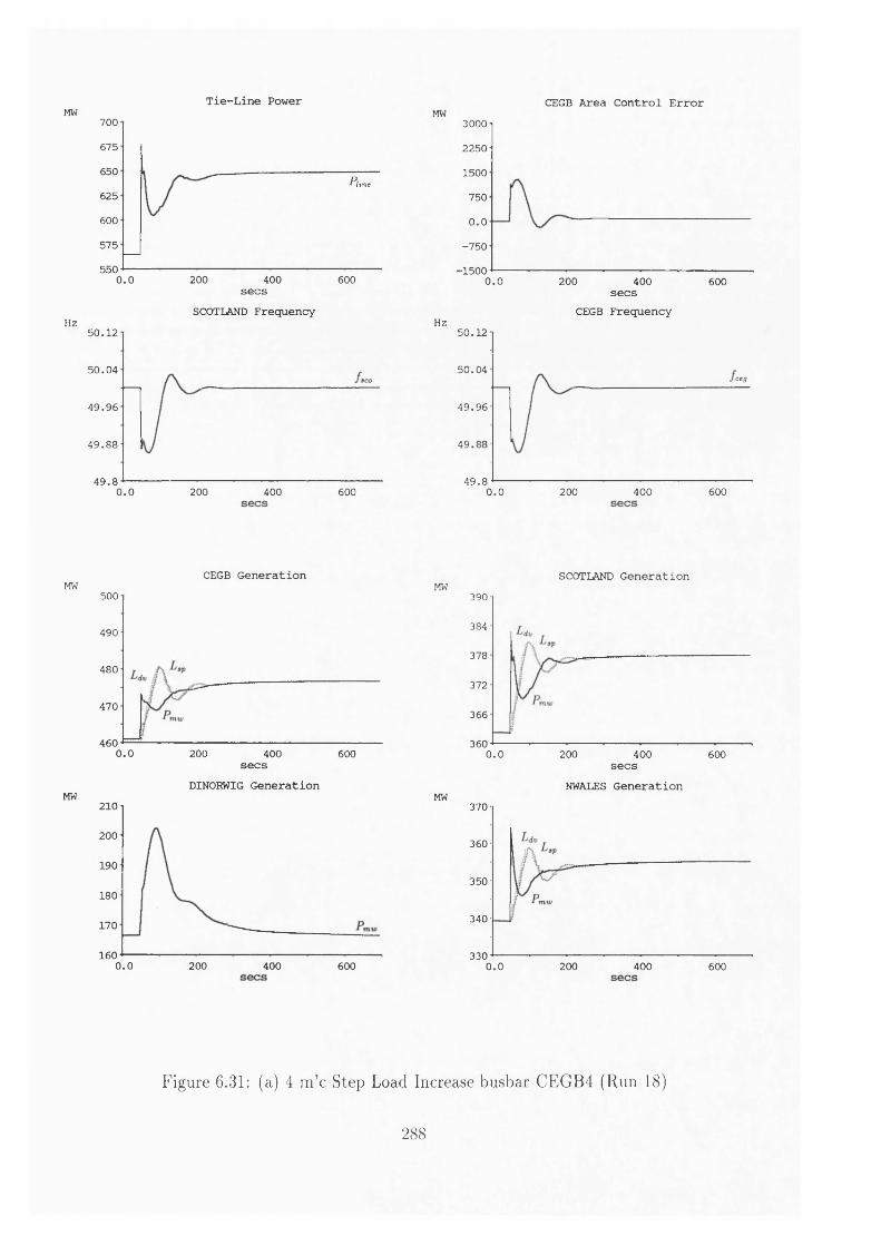
Tie-Line PowerMW 700
675
650P lin e
625
600
575
550 200 400 6000.0secs
SCOTLAND FrequencyHz
5 0 .1 2
5 0 .0 4
4 9 .9 6
4 9 .8 8
4 9 .80.0 200 400 600
CEGB Area Control ErrorMW 30002250
1500
750
0.0-7 5 0
■15000.0 200 400 600secs
CEGB FrequencyHz
50 .12
50 .0 4ceg
4 9 .9 6
49
4 9 .80.0 200 400 600
CEGB GenerationMW
MW
500
490
480
470
4600.0 200 400 600secs
DINOKWIG Generation210
200
190
180
170
1600.0 200 400 600
SCOTLAND GenerationMW
MW
390
384
378
372
366
3600.0 200 400 600secs
NWALES Generation370
360
350
340
3300.0 200 400 600
Figure 6.31: (a) 4 m ’c Step Load Increase busbar CEGB4 (Run 18)
288

I Co-')
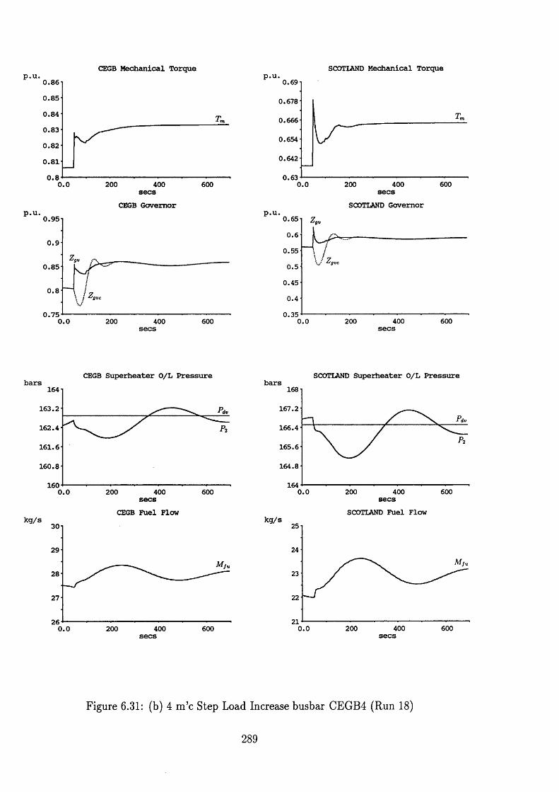
CEGB Mechanical Torque0.860 .8 5
0 .8 4
0 .8 3
0 .8 2
0 .8 1
0 .80.0 200 400 600
secs CEGB Governor
0 .9 5
0 .9
0 .8 5
0.8
0 .7 50.0 200 400 600
SCOTLAND Mechanical Torque0.69
0.678
0.666
0.654
0.642
0 .636000.0 200 400
secsSCOTLAND Governor
0 .65 <gv
0.60.55
0 .5
0.45
0 .4
0 .35600200 4000.0
CEGB Superheater O/L Pressurebars164
163.2 P d v
162 .4
161 .6
160 .8
1600.0 400 600200secs
CEGB Fuel Flow30
29
28
27
26400 6000.0 200
SCOTLAND Superheater O/L Pressurebars168
167.2
166.4
165.6
164.8
164400 6000.0 200 secs
SCOTLAND Fuel Flow
21400 6000.0 200
Figure 6.31: (b) 4 m ’c Step Load Increase busbar CEGB4 (Run 18)
289

% ( & , ( \ ^
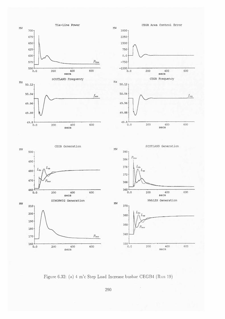
Tie-Line PowerMW 700
675
650
625
600
575
550600200 4000 .0 secs
SCOTLAND Frequency5 0 .1 2
5 0 .0 4
4 9 .9 6
4 9 .8 8
4 9 .86004000.0 200
CEGB Area Control ErrorMW 3000
2250
1500
750
0.0-7 5 0
-1 5 0 0400 6000.0 200
secs CEGB Frequency
Hz50 .12
50 .04ceg
4 9 .9 6
49.
4 9 .8 200 400 6000.0
CEGB Generation
200 400 600secs
330 -------------------------0 .0 200 400 600
secs
200 400 600secs
DINORWIG Generation
SCOTLAND Generation
200 400 600secs
NWALES Generation
378
372
Figure 6.32: (a) 4 m ’c Step Load Increase busbar CEGB4 (Run 19)
290
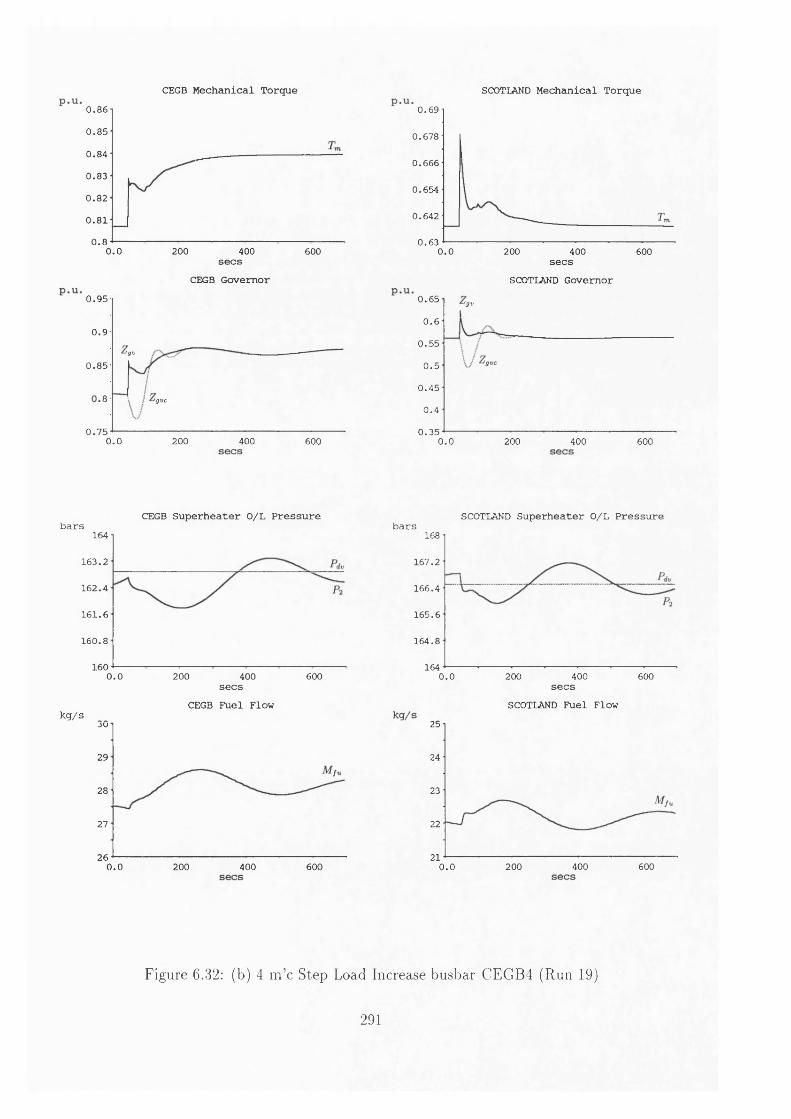
CEGB Mechanical Torque SCOTLAND Mechanical Torque0.860 .8 5
0 .8 4
0 .8 3
0 .8 2
0 .8 1
0.80.0 200 400 600secs
CEGB Governor0 .9 5
0 .9
lgV0 .8 5
8 Igvc
0 .7 50.0 200 400 600
0.69
0 .6 7 8
0 .6 6 6
0 .6 5 4
0 .642
0 .6 30.0 200 400 600secs
SCOTLAND Governor0 .6 5 'gv
0.60 .5 5
0 .5
0 .4 5
0 .4
0 .3 50.0 200 400 600
CEGB Superheater O/L Pressurebars
164
1 6 3 .2
16 2 .4
1 6 1 .6
16 0 .8
1600.0 200 400 600secs
CEGB Fuel Flowkg/s JU
29
28
27
260.0 200 400 600
SCOTLAND Superheater O/L Pressurebars
168
167 .2
166 .4
165 .6
164 .8
1640.0 200 400 600secs
SCOTLAND Fuel Flow25
24
23
22
210.0 200 400 600
Figure 6.32: (b) 4 m ’c Step Load Increase busbar CEGB4 (Run 19)
291

k c \
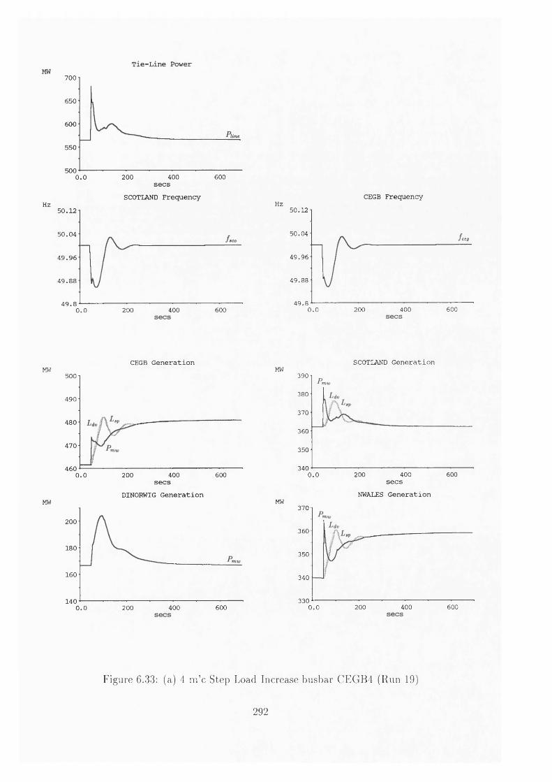
Tie-Line Power700
650
600
550
500200 400 6000.0
secsSCOTLAND Frequency
Hz5 0 .1 2
5 0 .0 4
4 9 .9 6
4 9 .8 8
4 9 .86000.0 200 400
CEGB Frequency Hz
50 .12
5 0 .04ceg
4 9 .9 6
4 9 .88
4 9 .8600200 4000.0
CEGB Generation MW
500
490
480 '*p
470
4600 .0 400 600200
secsDINORWIG Generation
MW
200
180
160
1406000.0 200 400
SCOTLAND Generation MW
390
380
370
360
350
3400 .0 200 400 600
secsNWALES Generation
MW370
360
350
340
3300 .0 200 400 600
Figure 6.33: (a) 4 m ’c Step Load Increase busbar CEGB4 (Run 19)
292

lo
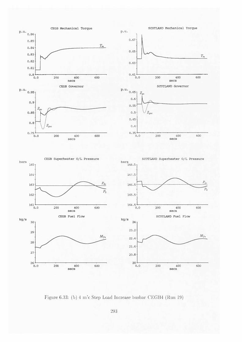
CEGB Mechanical Torque0.860 .8 5
0 .8 4
0 .8 3
0 .8 2
0 .8 1
0 .80 .0 200 400 600
secs CEGB Governor
SCOTLAND Mechanical Torquep.u.
0 .6 7
0 .6 5
0 .63
0 .6 1400 6000.0 200
secsSCOTLAND Governor
0 .6 5
0 . 6
0 .5 5
0 .5
0 .4 5
0 .4
0 .3 5400 6000.0 200
CEGB Superheater O/L Pressurebars
165
164
163
162
1610.0 200 400 600secs
CEGB Fuel Flow30
29
28
27
260.0 200 400 600
SCOTLAND Superheater O/L Pressure bars
1 6 8 .5
1 6 7 .5
dv1 6 6 .5
1 6 5 .5
16 4 .50.0 600200 400secs
SCOTLAND Fuel Flow
2 3 .2
2 2 .4
2 1 .6
20
6000.0 200 400
Figure 6.33: (b) 4 m ’c Step Load Increase busbar CEGB4 (Run 19)
0 .7 5 -400
secs
293

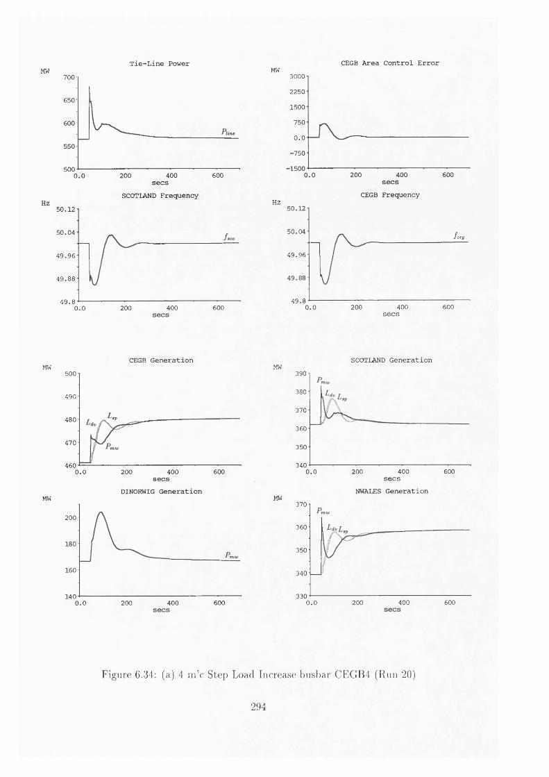
Tie-Line PowerMW 700
650
600
550
500400 6000.0 200
secsSCOTLAND Frequency
5 0 .1 2
5 0 .0 4
4 9 .9 6
4 9 .8 8
4 9 .8600200 4000.0
CEGB Area Control ErrorMW 3000
2250
1500
750
0.0•750
■1500400 6000.0 200
secs CEGB Frequency
Hz50 .12
50 .04c e g
4 9 .9 6
4 9 .8400 6000.0 200
secs
CEGB Generation MW
500
490
‘•p480
470
4600.0 200 400 600secs
DINORWIG GenerationMW
200
180
160
1406000.0 200 400
SCOTLAND Generation MW
390
380
370
360
350
3400 .0 200 400 600
secsNWALES Generation
MW370
360
350
340
3300 .0 200 400 600
Figure 6.34: (a) 4 m ’c Step Load Increase busbar CEGB4 (Run 20)
294

L ° C a .
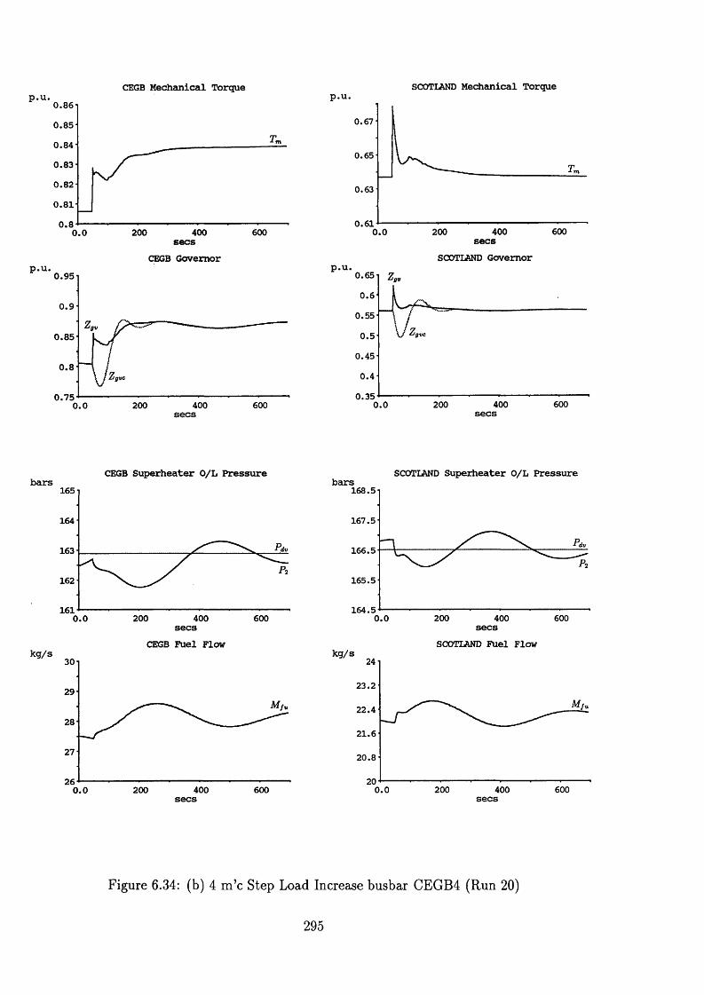
CEGB Mechanical Torque0.860 .8 5
0 .84
0 .83
0 .8 2
0 .8 1
0.8 200 400 6000.0 secs CEGB Governor
0 .9 5
0 .9
Igv
0 .8 5
0.8
0 .7 5400 6002000.0
SCOTLAND Mechanical Torquep . u .
0.67
0.65
0.63
0 .61400 6002000.0 secs
SCOTLAND Governor0 .65 tgv
0.60.55
0 .5 IgV C
0.45
0 .4
0 .35400 6000.0 200
CEGB Superheater O/L Pressure bars165
164
163
162
161400200 6000.0 secs
CEGB Fuel Flow30
29
28
27
264000.0 200 600
SCOTLAND Superheater O/L Pressure bars168.5
167.5
166.5
165.5
164.5 200 400 6000.0 secsSCOTLAND Fuel Flow
23.2
22.4
21.6
20.8
20400 6000.0 200
Figure 6.34: (b) 4 m ’c Step Load Increase busbar CEGB4 (Run 20)
295

® . ' i u C 'O )— '
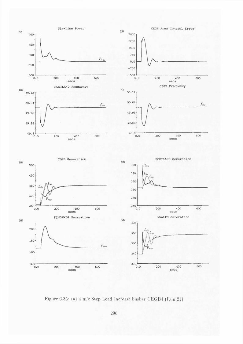
Tie-Line Power CEGB Area Control ErrorMW 700
650
600line
550
500400 6000.0 200
HZ
secsSCOTLAND Frequency
50.12
50.04
49.96
49.88
49.8600200 4000.0
MW 30002250
1500
750
0.0■750
-15000.0 200 400 600
Hz
secs CEGB Frequency
50.12
50.04ceg
49.96
49.88
49.8400 6002000.0
CEGB Generation SCOTLAND GenerationMW
MW
500
490
480
470
4600.0 200 400 600secs
DINORWIG Generation
200
180
160
140400 6000.0 200
MW
MW
390
380
370
360
350
340400 6000.0 200
secsNWALES Generation
370
360
350
340
330400 6000.0 200
secs
Figure 6.35: (a) 4 m ’c Step Load Increase busbar CEGB4 (Run 21)
296

o
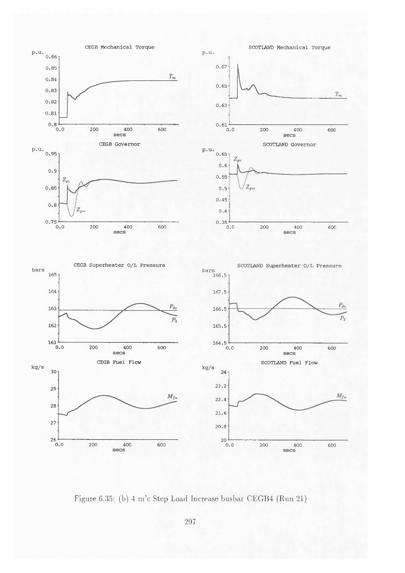
p.u.
bars
kg/s
CEGB Mechanical Torque0.860 .8 5
0 .8 4
0 .8 3
0 .8 2
0 .8 1
0.80.0 200 400 600secs
CEGB Governor0 .9 5
0 .9
'gv
0 .8 5
0.8'gvc
0 .7 50.0 200 400 600
SCOTLAND Mechanical Torquep.u.
0 .6 7
0 .6 5
0 .6 3
0 .6 10.0 200 400 600secs
SCOTLAND Governor0 .6 5
0.60 .5 5
0 .5
0 .4 5
0 .4
0 .3 50.0 200 400 600
CEGB Superheater O/L Pressure165
164
163
162
1610.0 200 400 600secs
CEGB Fuel Flow30
29
28
27
260.0 200 400 600
SCOTLAND Superheater O/L Pressurebars1 6 8 .5
1 6 7 .5
1 6 6 .5
1 6 5 .5
1 6 4 .50.0 200 400 600secs
SCOTLAND Fuel Flowkg/s
2 3 .2
2 2 .4
21.6
20.8
200.0 200 400 600
Figure 6.35: (b) 4 m ’c Step Load Increase busbar CEGB4 (Run 21)
297

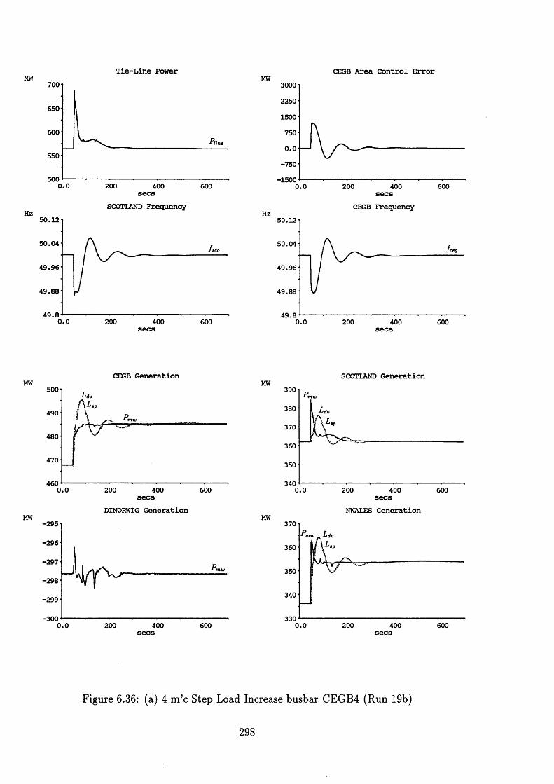
Tie-Line PowerMW 700
650
600
550
5000.0 200 400 600secs SCOTLAND Frequency Hz
50 .12
50 .04
4 9 .96
49 .88
4 9 .80.0 200 400 600
CEGB Area Control ErrorMW 30002250
1500
750
0.0-750
■1500400 6000.0 200 secs
CEGB Frequency Hz50.12
50.04
49 .96
49.88
4 9 .80.0 200 400 600
CEGB Generation MW500
490
480
470
4600.0 200 400 600secs DINORWIG Generation MW
-295
-296
■297
-298
-299
-300 200 4000.0 600
SCOTLAND Generation MW390
380
370
360
350
3400.0 200 400 600secs NWALES Generation MW
370
360
350
340
330 200 400 6000.0
Figure 6.36: (a) 4 m ’c Step Load Increase busbar CEGB4 (Run 19b)
298

OR

CEGB Mechanical Torque0.860 .8 5
0 .8 4
0 .8 3
0 .8 2
0 .8 1
0.80.0 200 400 600secs
CEGB Governor0 .9 5
*gv0 .9
0 .8 5 'gvc
0.8
0 .7 50.0 200 400 600
SCOTLAND Mechanical Torquep . u .
0 .67
0 .65
0.63
0 .610.0 200 400 600secsSCOTLAND Governor
0 .65 fg V
0.60.55
0 .5 'gvc
0 .45
0 .4
0 .350.0 200 400 600
CEGB Superheater O/L Pressure bars165
164
163P d v
162
1610.0 200 400 600secsCEGB Fuel Flow
30
29
28
27
260.0 200 400 600
SCOTLAND Superheater O/L Pressure bars168.5
167.5
166.5
165.5
164.50.0 200 600400secsSCOTLAND Fuel Flowkg/s
23.2
22.4
21.6
20.8
0.0 200 400 600
Figure 6.36: (b) 4 m ’c Step Load Increase busbar CEGB4 (Run 19b)
299

\q)
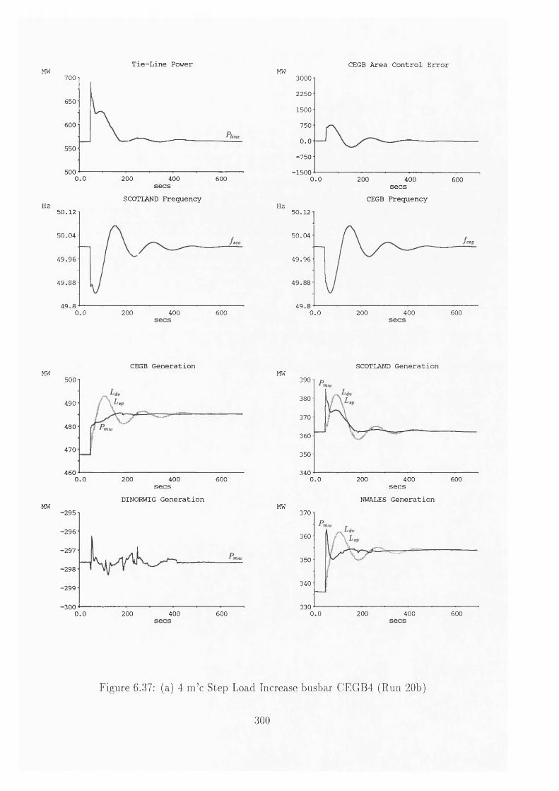
Tie-Line Power CEGB Area Control ErrorMW MW700
650
600
550
5000.0 200 400 600
Hz
secsSCOTLAND Frequency
50 .1 2
50 .04
4 9 .9 6
4 9 .8 8
4 9 .80.0 200 400 600
30002250
1500
750
0.0-7 5 0
•15000.0 200 400 600
Hz
secs CEGB Frequency
50 .12
50 .04
4 9 .9 6
49 0.0 200 400 600
CEGB Generation SCOTLAND GenerationMW
MW
500
490
480
470
4600.0 200 400 600
secsDINOKWIG Generation
•295
•296
-2 9 7
•298
-2 9 9
•3004000.0 200 600
MW
MW
390
380
370
360
350
340400 6000.0 200
secsNWALES Generation
370
360
350
340
3300.0 200 400 600
Figure 6.37: (a) 4 m ’c Step Load Increase busbar CEGB4 (Run 20b)
300

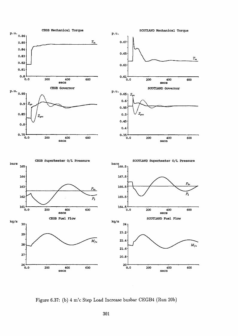
CEGB Mechanical Torque0.860 .8 5
0 .8 4
0 .8 3
0 .8 2
0 .8 1
0.80.0 400200 600
secsCEGB Governor
0 .9 5
0 .9 fgV
0 .8 5tgV C
0.8
0 .7 50.0 200 400 600
SCOTLAND Mechanical Torquep.u.
0 .67
0 .6 5
0 .6 3
0 .6 10.0 200 400 600secsSCOTLAND Governor
0 .6 5 Ig V
0 . 6
0 .5 5
0 .5
0 .4 5
0 .4
0 .3 50.0 200 400 600
CEGB Superheater O/L Pressure bars165
164
163
162
1612000.0 400 600secs
CEGB Fuel Flow30
29
28
27
260.0 200 400 600
SCOTLAND Superheater O/L Pressure bars1 6 8 .5
16 7 .5
166 .5
16 5 .5
16 4 .50 .0 200 400 600
secsSCOTLAND Fuel Flow
24
2 3 .2
2 2 .4
2 1 .6
20.8
200.0 400 600200
Figure 6.37: (b) 4 m ’c Step Load Increase busbar CEGB4 (Run 20b)
301

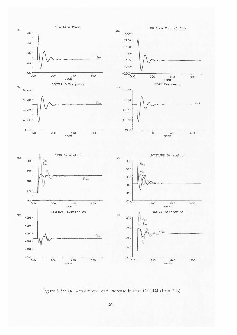
MW
Hz5 0 .1 2
4 9 .80.0
Tie-Line Power700
650
600P lin e
550
5000.0 200 400 600secs
SCOTLAND Frequency
200 400secs
600
MW CEGB Area Control Error30002250
1500
750
0.0
■750
•15000.0 200 400 600
HZ
secs CEGB Frequency
5 0 .1 2
5 0 .0 4ceg
4 9 .9 6
4 9 .8 8
4 9 .80.0 200 400 600
CEGB Generation500
490
480
470
4600.0 200 400 600secs
DINORWIG Generation■295
-2 9 6
■297
-298
-299
■3000.0 200 400 600
SCOTLAND GenerationMW390
380
fti,370
360
350
3400 .0 200 400 600
secsNWALES Generation
370
360
350
340
3300 .0 200 400 600
Figure 6.38: (a) 4 m ’c Step Load Increase busbar CEGB4 (Run 21b)
5 0 .0 4
4 9 .9 6
4 9 .8 8
302

CEGB Mechanical Torque0.860 .8 5
0 .8 4
0 .8 3
0 .8 2
0 .8 1
0.8 200 400 6000.0secs
CEGB Governor0 .9 5
lgv0 .9
0 .8 5‘gvc
0 .7 5400 6000.0 200
SCOTLAND Mechanical Torquep.u.
0 .6 7
0 .6 5
0 .6 3
0 .6 1600200 4000.0
secsSCOTLAND Governor
0 .6 5lgv
0.60 .5 5
0 .5
0 .4 5
0 .4
0 .3 5600200 4000.0
CEGB Superheater O/L Pressurebars
165
164
163
162
161400 6000.0 200
secs CEGB Fuel Flow
30
600200 4000.0
SCOTLAND Superheater O/L Pressurebars
16 8 .5
1 6 7 .5
1 6 6 .5
1 6 5 .5
1 6 4 .5600200 4000.0 secs
SCOTLAND Fuel Flow
2 3 .2
2 2 .4
2 1 .6
20 6004000.0 200
Figure 6.38: (b) 4 m ’c Step Load Increase busbar CEGB4 (Run 21b)
303

9, ( «cT)
Tie-Line PowerMW 700
650
600
550
5000.0 200 400 600secsSCOTLAND FrequencyHz
50.12
50.04
49 .96
49 .88
4 9 .80.0 200 400 600
CEGB Area Control ErrorMW 3000
2250
1500
750
0.0-750
-15006004002000.0 secs
CEGB FrequencyHz50.12
50.04ceg
49.96
49.88
49 .80.0 200 400 600
CEGB GenerationMW
500
490
480
470
460 200 400 6000.0 secsDINOKWIG Generation
MW-295
-296
-297
-298
-299
■3000.0 400 600200
SCOTLAND GenerationMW
390
380
370
360
350
3406004000.0 200 secs
NWALES GenerationMW
370
360
350
340
330 600200 4000.0
Figure 6.39: (a) 4 m ’c Step Load Increase busbar CEGB4 (Run 22b)
304

(e? .^ P l (Ca)
p.u.
bars
kg/s
CEGB Mechanical Torque SCOTLAND Mechanical Torque
0.8400 6000.0 200
secs CEGB Governor
0 .9 <gv
•gvc
6000.0 200 400
p.u.
0 .6 7
0 .6 5
0 .6 3
0 .6 1400 6000.0 200
secsSCOTLAND Governor
p.u.0 .6 5
lgv
0.60 .5 5
0 .5 'gvc
0 .4 5
0 .4
0 .3 5400 6000.0 200
CEGB Superheater O/L Pressure165
164
163dv
162
161 200 400 6000.0secs
CEGB Fuel Flow30
29
28
27
260.0 200 400 600
barsSCOTLAND Superheater O/L Pressure
1 6 8 .5
16 7 .5
1 6 6 .5
1 6 5 .5
1 6 4 .56004000.0 200
kg/s
secsSCOTLAND Fuel Flow
2 3 .2
2 2 .4
2 1 .6
20
20400 6002000.0
Figure 6.39: (b) 4 m ’c Step Load Increase busbar CEGB4 (Run 22b)
305

'^Zlo ^
Tie-Line PowerMW 700
650
600
550
500400200 6000.0 secs
SCOTLAND FrequencyHz50.12
50.04
49 .96
49 .88
4 9 .86000.0 400200 secs
CEGB GenerationMW500
490
480
470
460 200 400 6000.0 secsDINOKWIG GenerationMW
200
180
160
140400 6000.0 200
CEGB Area Control ErrorMW 30002250
1500
750
0.0-750
-15000.0 200 400 600secs CEGB Frequency
Hz50.12
50.04
49 .96
49.88
49 .86000.0 200 400secs
SCOTLAND GenerationMW390
380
370
360
350
340400 6000.0 200
secsNWALES GenerationMW
370
360
350
340
330400 6000.0 200
Figure 6.40: (a) 4 m ’c Step Load Increase busbar CEGB4 (Run 23)
306

l^o C°^)
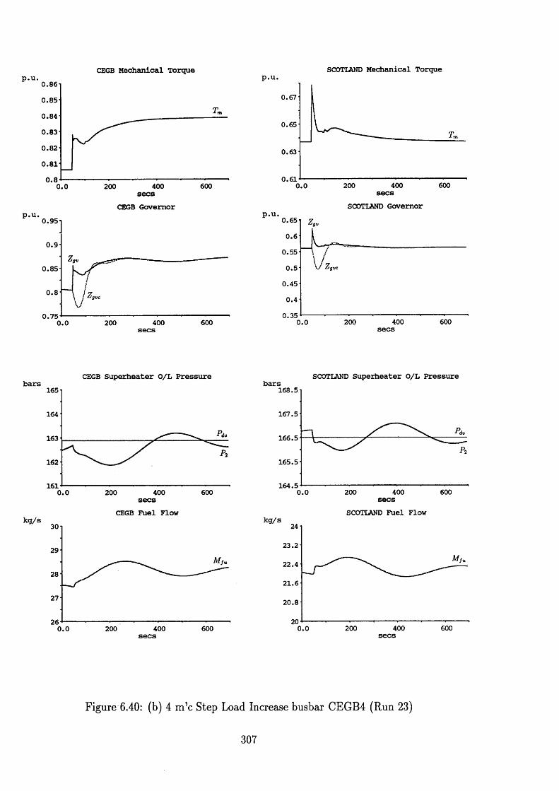
CEGB Mechanical Torque0.860 .8 5
0 .8 4
0 .8 3
0 .8 2
0 .8 1
0.86004000.0 200 secs
CEGB Governor0 .9 5
0 .9
IgV
0 .8 5
0.8
0 .7 56004002000.0
SCOTLAND Mechanical Torquep . u .
0 .67
0.65
0.63
0 .616004002000.0 secs
SCOTLAND Governor0 .65
0 .6
0 .55
0 .5 i g vc
0.45
0 .4
0 .356004002000.0
CEGB Superheater O/L Pressurebars165
164
163
162
1614000.0 200 600
secsCEGB Fuel Flow
30
29
28
27
266000.0 400200
SCOTLAND Superheater O/L Pressurebars
168.5
167.5
166.5
165.5
164.56004000.0 200
secsSCOTLAND Fuel Flow
23.2
22.4
21 .6
20 .8
400 6000.0 200
Figure 6.40: (b) 4 m ’c Step Load Increase busbar CEGB4 (Run 23)
307

Lfk - - -> • ^ c ^o . 1+0 C0 )
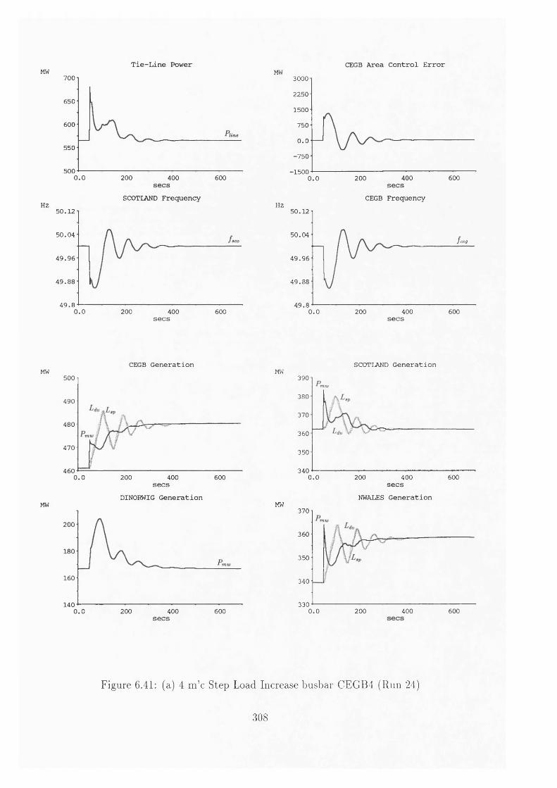
Tie-Line PowerMW 700
650
600
550
5000 .0 200 400 600
secsSCOTLAND Frequency
Hz5 0 .1 2
5 0 .0 4
4 9 .9 6
4 9 .8 8
4 9 .80.0 200 400 600secs
CEGB Generation MW
500
490
480
470
4600.0 200 400 600secs
DINORWIG Generation MW
200
180
160
1400 . 0 200 400 600
secs
CEGB Area Control ErrorMW 3000
2250
1500
750
0.0■750
•1500600200 4000 .0 secs
CEGB FrequencyHz
5 0 .1 2
5 0 .0 4ctg
4 9 .9 6
4 9 .8 8
4 9 .80.0 200 400 600secs
SCOTLAND GenerationMW390
380
370
360
350
3400.0 200 400 600
secsNWALES Generation
MW370
360
350
340
3300.0 200 400 600
Figure 6.41: (a) 4 m ’c Step Load Increase busbar CEGB4 (Run 24)
308

o
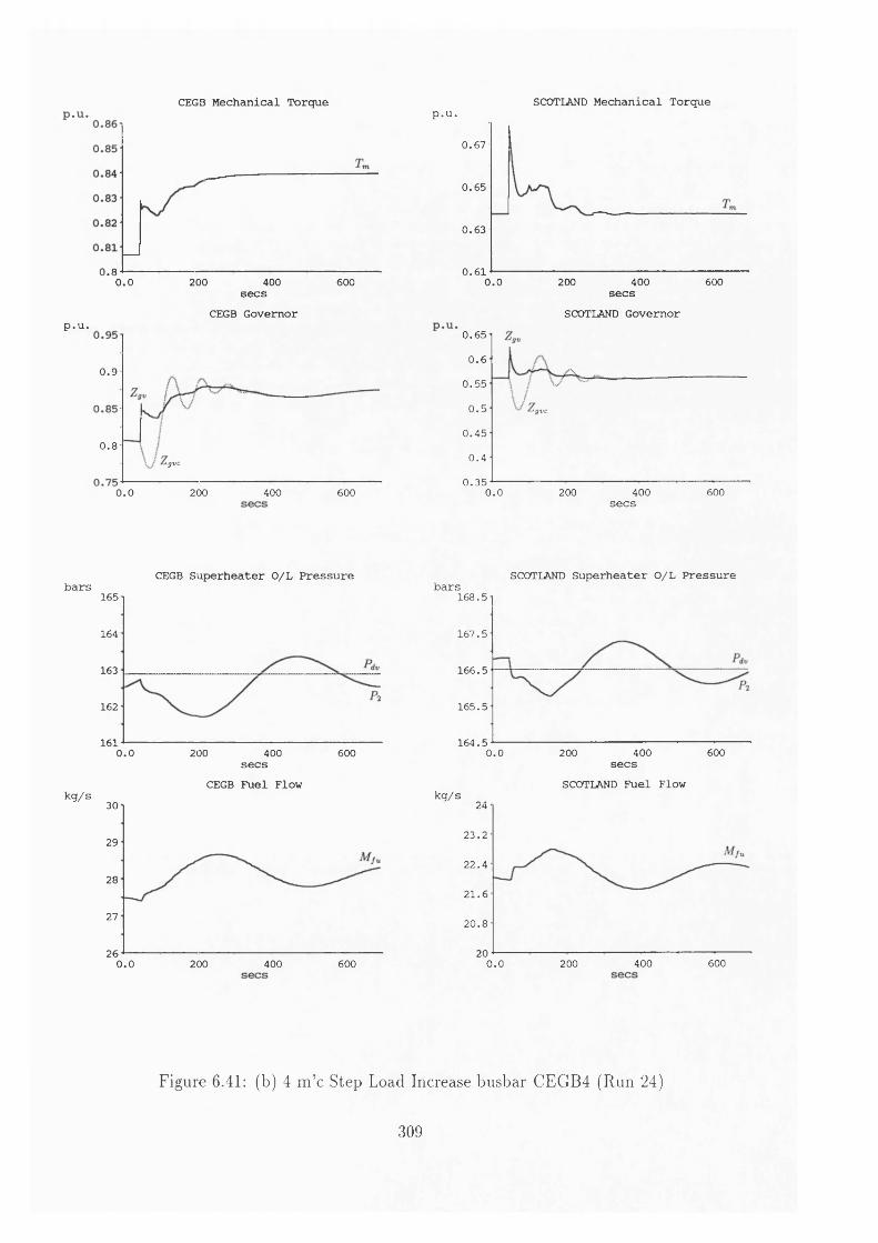
p.u.
bars
kg/s
CEGB Mechanical Torque
0.8400 6000.0 200
secs CEGB Governor
0 .9
0.8I gvC
0.0 200 400 600
SCOTIAND Mechanical Torquep.u.
0 .6 7
0 .6 5
0 .6 3
0 .6 10.0 200 400 600secs
SCOTLAND Governor0 .6 5
0.60 .5 5
0 .5 'gvc
0 .4 5
0 .4
0 .3 56000.0 200 400
secs
CEGB Superheater O/L Pressure165
164
163
162
1610.0 600200 400secs
CEGB Fuel Flow30
29
28
27
260.0 200 400 600
SCOTLAND Superheater O/L Pressurebars
1 6 8 .5
1 6 7 .5
16 6 .5
16 5 .5
16 4 .50.0 200 400 600secs
SCOTLAND Fuel Flowkg/s
/.‘k
2 3 .2
2 2 .4
21.6
20.8
20 6000.0 200 400
Figure 6.41: (b) 4 m ’c Step Load Increase busbar CEGB4 (Run 24)
309

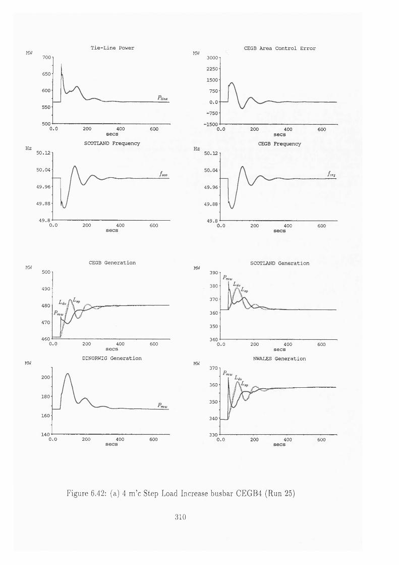
Tie-Line PowerMW 700
650
600
550
5000.0 200 400 600secs
SCOTLAND Frequency Hz5 0 .1 2
5 0 .0 4
4 9 .9 6
4 9 .8 8
4 9 .80.0 200 400 600
CEGB Area Control ErrorMW 30002250
1500
750
0.0•750
•15000.0 200 400 600secs
CEGB Frequency Hz50 .12
50 .0 4ceg
4 9 .9 6
4 9 .8 8
4 9 .80.0 200 400 600
CEGB GenerationMW500
490
480
470
4600.0 200 400 600secs
DINORWIG GenerationMW
200
180
160
1400.0 200 400 600
SCOTLAND GenerationMW390
380
370
360
350
3400 .0 200 400 600
secsNWALES GenerationMW
370
360
350
340
3300 .0 200 400 600
Figure 6.42: (a) 4 m ’c Step Load Increase busbar CEGB4 (Run 25)
310
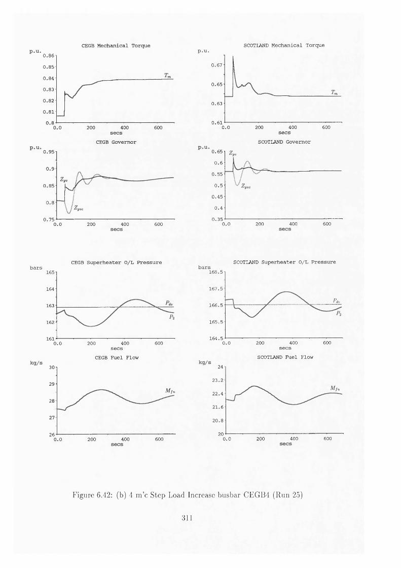
CEGB Mechanical Torque0 .86
0 .8 5
0 .8 4
0 .8 3
0 .8 2
0 .8 1
0.84000.0 200 600
secs CEGB Governor
0 .9 5
0 .9
0 .8 5
0.8
0 .7 5 200 400 6000.0
SCOTLAND Mechanical Torquep.u.
0 .6 7
0 .6 5
0 .6 3
0 .6 1400 6000.0 200
secsSCOTLAND Governor
0 .6 5
0.60 .5 5
0 .5
0 .4 5
0 .4
0 .3 56000.0 200 400
CEGB Superheater O/L Pressurebars
165
164
163
162
1616000.0 200 400
secsCEGB Fuel Flow
30
29
28
26400 6000.0 200
SCOTLAND Superheater O/L Pressurebars
1 6 8 .5
1 6 7 .5
Pdv1 6 6 .5
1 6 5 .5
1 6 4 .5 200 400 6000.0secs
SCOTLAND Fuel Flow24
2 3 .2
2 2 .4
21.6
20.8
20 600200 4000.0
Figure 6.42: (b) 4 m ’c Step Load Increase busbar CEGB4 (Run 25)
311

C,
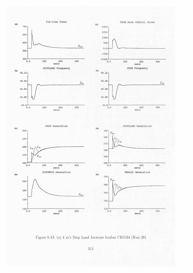
Tie-Line PowerMW 700
650
600
550
5000.0 200 400 600secs
SCOTLAND Frequency5 0 .1 2
5 0 .0 4
4 9 .9 6
4 9 .8 8
4 9 .80.0 200 400 600secs
CEGB Generation MW
500
490
480
470
4600.0 200 400 600secs
DINORWIG Generation MW
200
180
160
1400.0 200 400 600
CEGB Area Control ErrorMW 30002250
1500
750
0.0•750
•15000.0 200 400 600secs
CEGB FrequencyHz
5 0 .1 2
5 0 .0 4ceg
4 9 .9 6
4 9 .8 8
4 9 .80.0 200 400 600secs
SCOTLAND Generation MW
390
380'dv
370
360
350
3400.0 200 400 600secs
NWALES Generation MW370
360
350
340
3300.0 200 400 600
Figure 6.43: (a) 4 m ’c Step Load Increase busbar CEGB4 (Run 26)
312

o
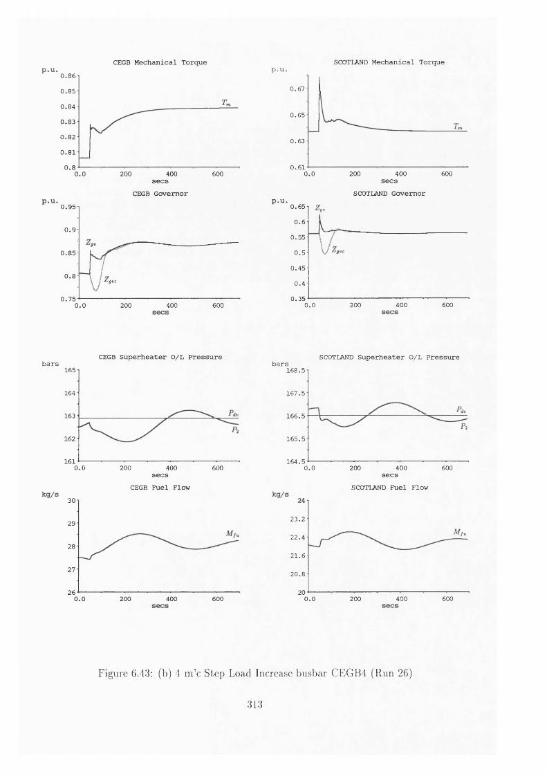
CEGB Mechanical Torque0.860 .8 5
0 .8 4
0 .8 3
0 .8 2
0 .8 1
0.84000.0 200 600
secs CEGB Governor
0 .9 5
0 .9
0 .8 5
0.8'gvc
0 .7 5400 6000.0 200
SCOTLAND Mechanical Torquep.u.
0 .6 7
0 .6 5
0 .6 3
0 .6 10.0 200 400 600secs
SCOTLAND Governor0 .6 5 'gv
0.60 .5 5
0 .5
0 .4 5
0 .4
0 .3 56000.0 200 400
CEGB Superheater O/L Pressurebars
165
164
163
162
1610 .0 200 400 600
secsCEGB Fuel Flow
30
29
28
27
260.0 200 400 600
SCOTLAND Superheater O/L Pressurebars
1 6 8 .5
1 6 7 .5
1 6 6 .5
1 6 5 .5
1 6 4 .5 200 400 6000.0secs
SCOTLAND Fuel Flow
2 3 .2
2 2 .4
21.6
20.8
200.0 200 400 600
Figure 6.43: (b) 4 m ’c Step Load Increase busbar CEGB4 (Run 26)
313

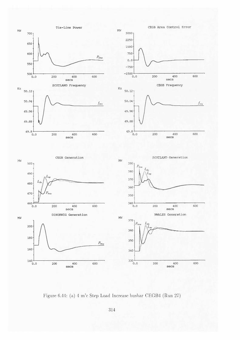
Tie-Line Power CEGB Area Control ErrorMW 700
650
600
550
500 200 400 6000.0
Hz
secsSCOTLAND Frequency
5 0 .1 2
5 0 .0 4
4 9 .9 6
4 9 .8 8
4 9 .8400 6000.0 200
MW 30002250
1500
750
0.0-7 5 0
■15006004000.0 200
Hz
secs CEGB Frequency
5 0 .1 2
5 0 .0 4ceg
4 9 .9 6
4 9 .8 8
4 9 .8400 6000.0 200
CEGB Generation SCOTLAND GenerationMW
MW
500
490
480
470
4600.0 200 400 600secs
DINOKWIG Generation
200
180
160
1400.0 200 400 600
MW
MW
390
380
370
360
350
3406000.0 200 400
secsNWALES Generation
370
360
350
340
330 6004000.0 200
Figure 6.44: (a) 4 m ’c Step Load Increase busbar CEGB4 (Run 27)
314

??■ pV \ b :
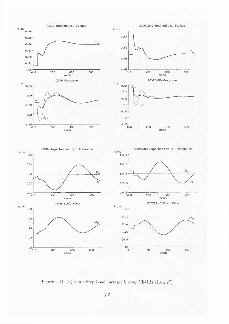
p.u.
bars
kg/s
CEGB Mechanical Torque SCOTLAND Mechanical Torque0.860 .8 5
0 .8 4
0 .8 3
0 .8 2
0 .8 1
0.8 200 400 6000.0secs
CEGB Governor0 .9 5
0 .9
0 .8 5
0.8<gvc
0 .7 5400 6000.0 200
p.u.
0 .6 7
0 .6 5
0 .6 3
0 .6 16000.0 200 400
secsSCOTLAND Governor
p.u.0 .6 5
0.60 .5 5
0 .5
0 .4 5
0 .4
0 .3 56000.0 200 400
CEGB Superheater O/L Pressure barsSCOTLAND Superheater 0/L Pressure
secs CEGB Fuel Flow
165
164
dv163
162
161400 6000.0 200
30
29
28
27
26600200 4000.0
16 8 .5
1 67 .5
1 6 6 .5
1 6 5 .5
164 .5400 6002000.0 secs
SCOTLAND Fuel Flowkg/s
2 3 .2
2 2 .4
21.6
20.8
20400 6000.0 200
Figure 6.44: (b) 4 m ’c Step Load Increase busbar CEGB4 (Run 27)
315

k-U rbo)
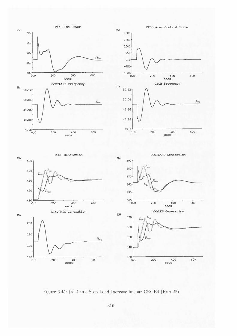
Tie-Line Power CEGB Area Control ErrorMW MW700
650
600
550
500400 6000.0 200
Hz
secsSCOTLAND Frequency
5 0 .1 2
5 0 .0 4
4 9 .9 6
4 9 .8 8
4 9 .86004000.0 200
30002250
1500
750
0.0-7 5 0
-1500400 6000 .0 200
HZ
secs CEGB Frequency
5 0 .12
5 0 .04
4 9 .9 6
49
4 9 .86004000.0 200
CEGB Generation SCOTLAND GenerationMW
MW
500
490
\ >480
470
460400 6000 .0 200
secsDINOKWIG Generation
200
180
160
140400 6000.0 200
MW
MW
390
A380
370
360 'dv \
350
3406000.0 200 400
secsNWALES Generation
370
360
350
340
330200 400 6000.0
Figure 6.45: (a) 4 m ’c Step Load Increase busbar CEGB4 (Run 28)
316

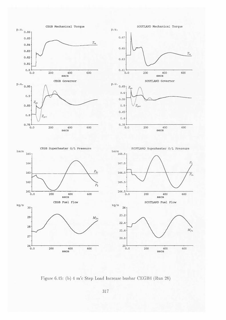
p.u.
bars
kg/s
CEGB Mechanical Torque
0.80.0 200 400 600secs
CEGB Governor
0 .9
0.8 igvc
0.0 200 400 600
p.U.SCOTLAND Mechanical Torque
0 .6 7
0 .6 5
0 .6 3
0 .6 1 200 400 6000.0secs
SCOTLAND Governorp.u.
0 .6 5
0 .6
0 .5 5
0 .5
0 .4 5
0 .4
0 .3 50.0 200 400 600
CEGB Superheater O/L Pressurebars SCOTLAND Superheater O/L Pressure
165
164
163
162
1610.0 200 400 600secs
CEGB Fuel Flow30
29
28
27
260.0 200 400 600
1 6 8 .5
1 6 7 .5
166 .5
1 6 5 .5
1 6 4 .50.0 200 400 600
kg/s
secsSCOTLAND Fuel Flow
2 3 .2
2 2 .4
21.6
2 0 .8
200.0 200 400 600
Figure 6.45: (b) 4 m ’c Step Load Increase busbar CEGB4 (Run 28)
317

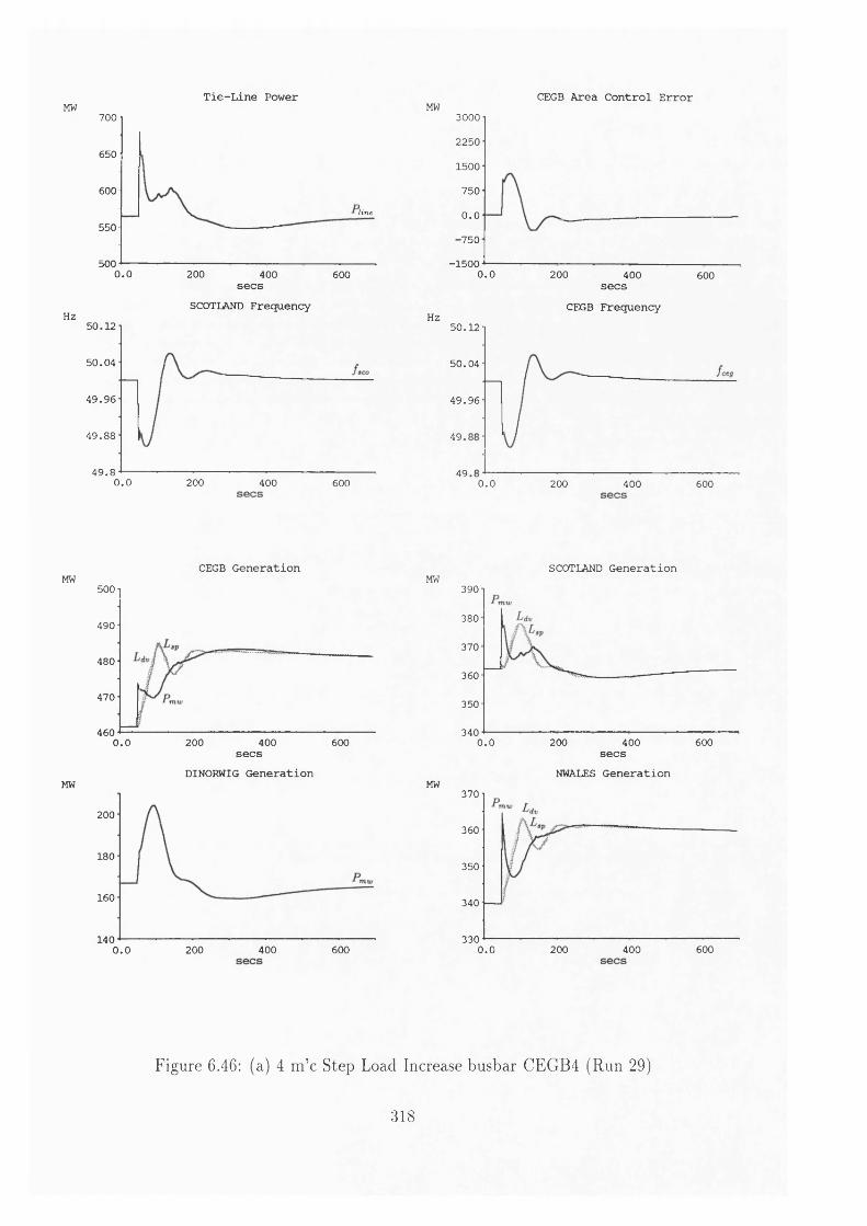
Tie-Line PowerMW 700
650
600
line
550
5000.0 200 400 600secs
SCOTLAND Frequency Hz
5 0 .1 2
5 0 .0 4
4 9 .9 6
4 9 .8 8
4 9 .80.0 200 400 600
CEGB Area Control ErrorMW 30002250
1500
750
0.0•750
-15 0 00.0 200 400 600secs CEGB FrequencyHz
50 .12
50 .04
4 9 .9 6
49
49 0.0 200 400 600
CEGB Generation MW
500
490
480
470
4600 .0 200 400 600
secsDINORWIG Generation
MW
200
180
160
1400 .0 200 400 600
SCOTLAND GenerationMW
390
380
370
360
350
3400 .0 200 400 600
secsNWALES Generation
MW370
360
350
340
3300 .0 200 400 600
Figure 6.46: (a) 4 m ’c Step Load Increase busbar CEGB4 (Run 29)
318

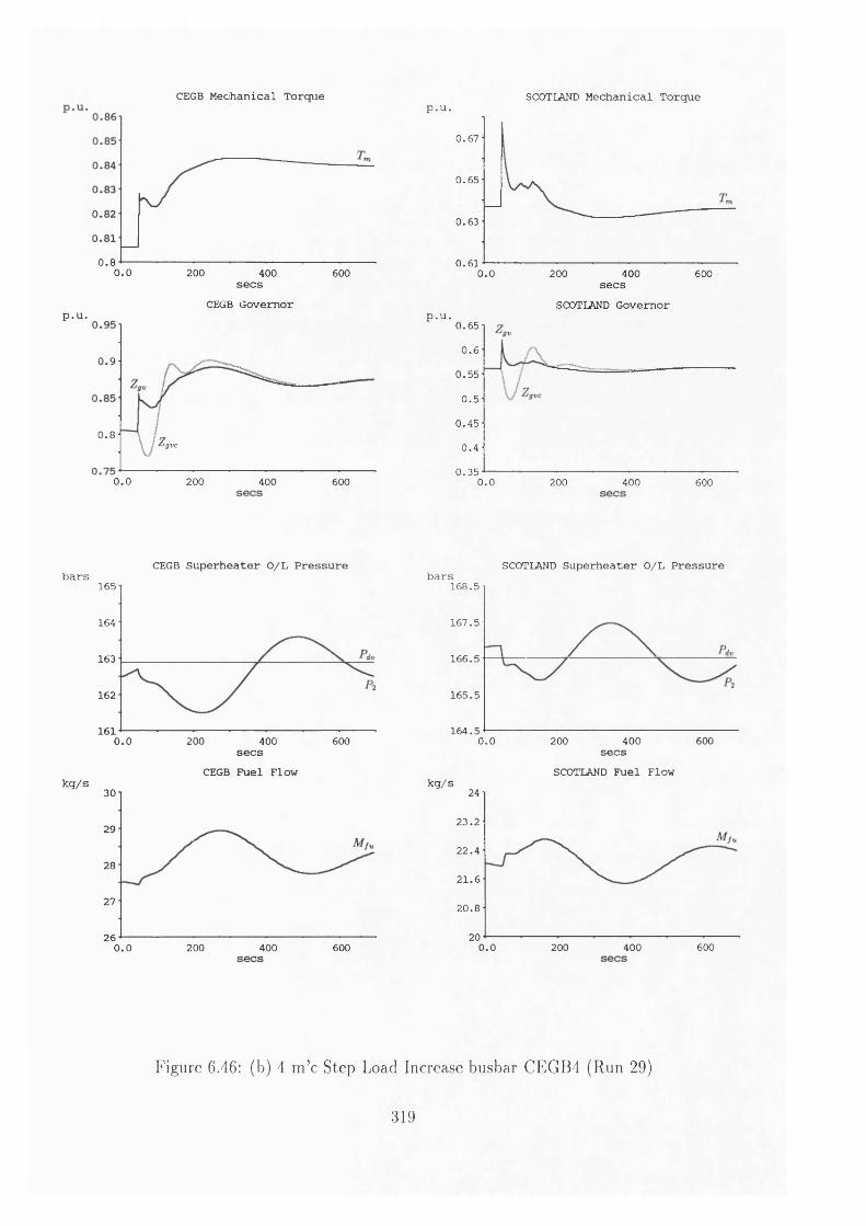
p.u.
bars
kg/s
CEGB Mechanical Torque
0 .80.0 200 400 600secs
CEGB Governor
0 .9
0.8'gvc
0.0 200 400 600
p.u.SCOTLAND Mechanical Torque
0 .6 7
0 .6 5
0 .6 3
0 .6 10.0 200 400 600secs
SCOTLAND Governorp.u.
0 .6 5
0.60 .5 5
0 .5
0 .4 5
0 .4
0 .3 50.0 200 400 600
CEGB Superheater O/L Pressurebars
SCOTLAND Superheater O/L Pressure165
164
163
162
1610.0 200 400 600secs
CEGB Fuel Flow30
29
28
27
260.0 200 400 600
1 6 8 .5
1 6 7 .5
1 6 6 .5
1 6 5 .5
1 6 4 .50.0 200 400 600
kg/s
secsSCOTLAND Fuel Flow
24
2 3 .2
2 2 .4
21.6
2 0 .8
200.0 200 400 600
Figure 6.46: (b) 4 m ’c Step Load Increase busbar CEGB4 (Run 29)
319

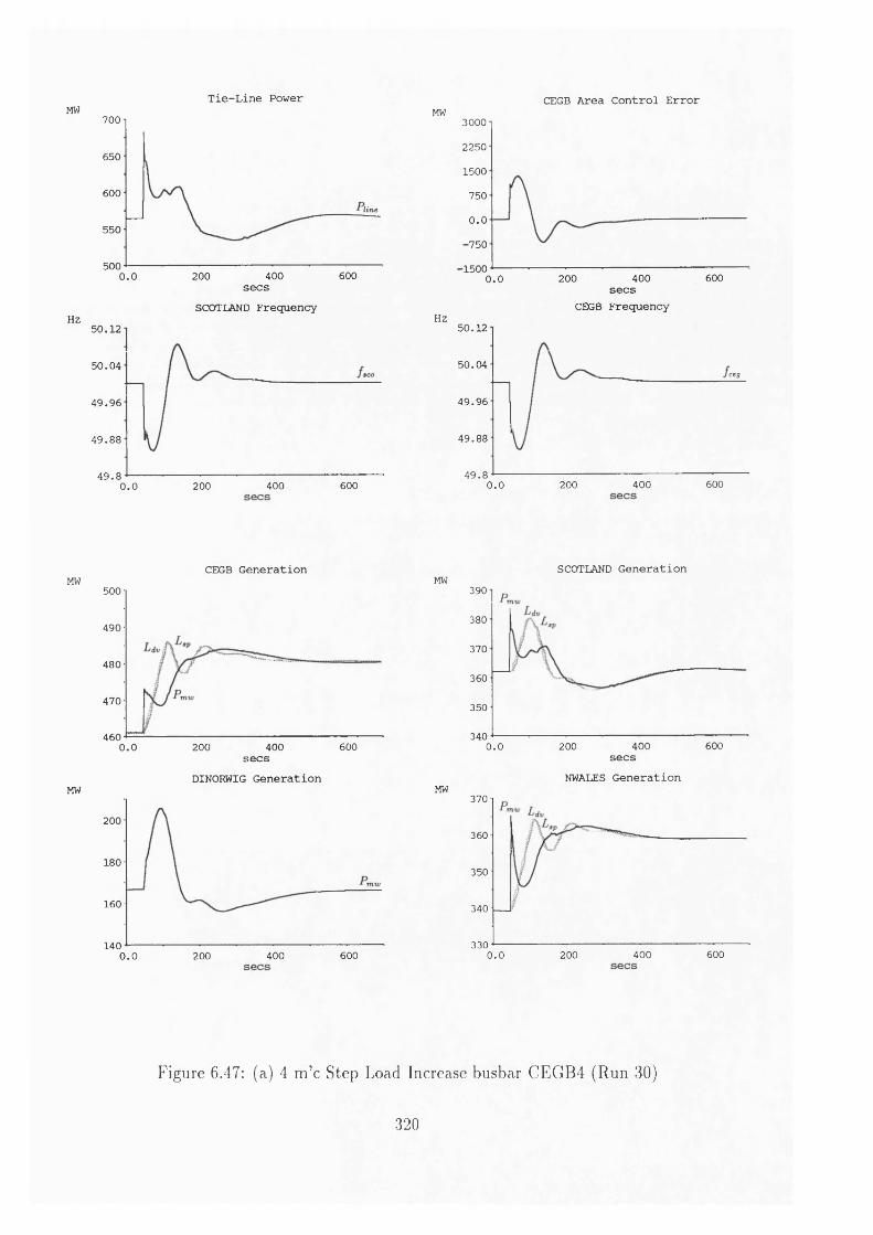
Tie-Line Power CEGB Area Control ErrorMW 700
650
600
550
500600200 4000.0
MW
Hz
secsSCOTLAND Frequency
5 0 .1 2
5 0 .0 4
4 9 .9 6
4 9 .8 8
4 9 .8400 6000.0 200
30002250
1500
750
0.0■750
■1500400 6002000.0
Hz
secs CEGB Frequency
5 0 .1 2
50 .0 4ceg
4 9 .9 6
4 9 .8 8
4 9 .8600200 4000.0
CEGB Generation SCOTLAND GenerationMW
MW
500
490
480
470
4600.0 200 400 600secs
DINORWIG Generation
200
180
160
1400.0 200 400 600
MW
MW
390
380
370
360
350
340400 6000.0 200
secsNWALES Generation
370
360
350
340
330 600200 4000.0
Figure 6.47: (a) 4 m ’c Step Load Increase busbar CEGB4 (Run 30)
320

5 0 ^ (c - ,4
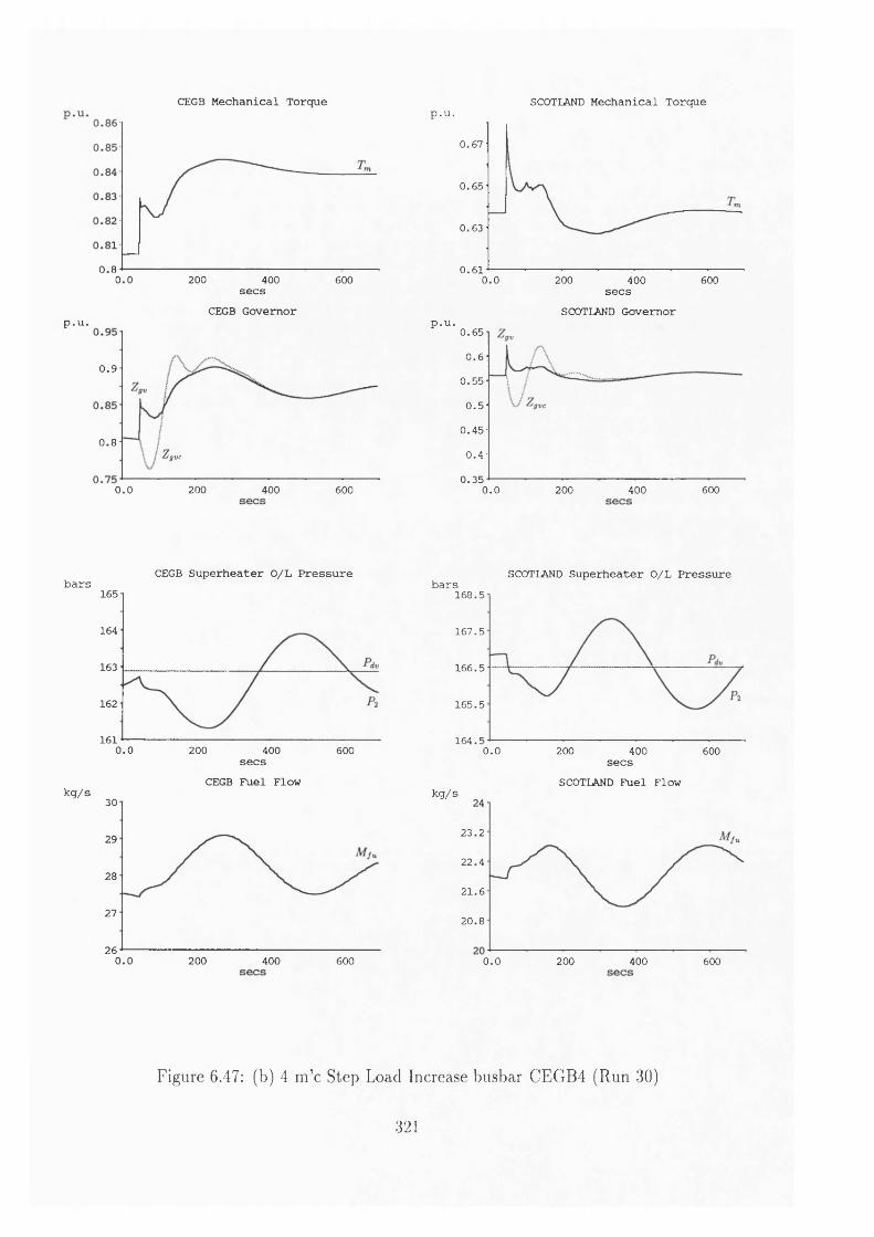
p.u.
bars
kg/s
CEGB Mechanical Torque
0.80 . 0 200 400 600
secs CEGB Governor
0 .9
0 . 8(JV C
0.0 200 400 600
p.u.SCOTLAND Mechanical Torque
0 .6 7
0 .6 5
0 .6 3
0 .6 10.0 200 400 600
p.u.
secsSCOTLAND Governor
0 .6 5
0.60 .5 5
0 .5
0 .4 5
0 .4
0 .3 50.0 600200 400
CEGB Superheater O/L Pressurebars SCOTLAND Superheater O/L Pressure
165
164
163
162
1610.0 200 400 600secs
CEGB Fuel Flow30
29
28
27
260.0 200 400 600
16 8 .5
1 6 7 .5
1 6 6 .5
1 6 5 .5
16 4 .50.0 200 400 600
kg/s
secsSCOTLAND Fuel Flow
2 3 .2
2 2 .4
2 1 .6
2 0 .8
0.0 200 400 600
Figure 6.47: (b) 4 m ’c Step Load Increase busbar CEGB4 (Run 30)
321

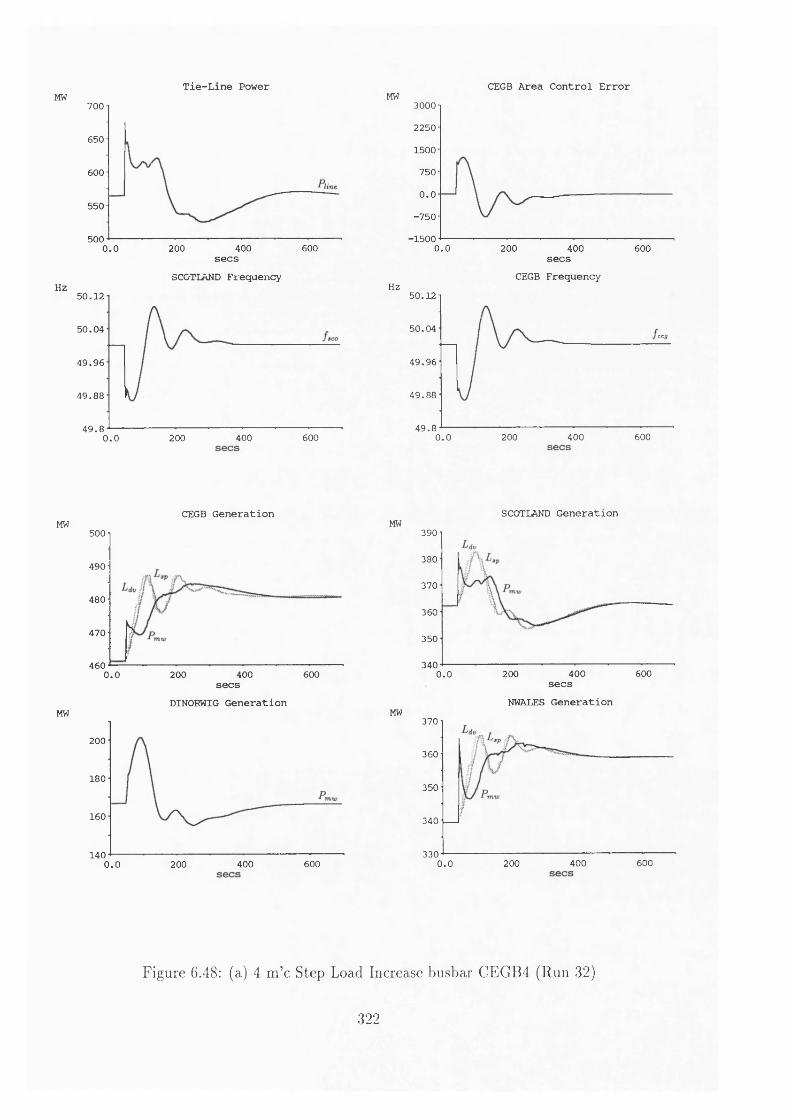
Tie-Line Power CEGB Area Control ErrorMW 700
650
600
550
500 200 400 6000.0
Hz
secsSCOTLAND Frequency
5 0 .1 2
5 0 .0 4
4 9 .9 6
4 9 .8 8
4 9 .8 200 400 6000.0
MW 30002250
1500
750
0.0-7 5 0
-1 5 0 00.0 200 400 600
Hz
secs CEGB Frequency
50 .1 2
50 .0 4ctg
4 9 .9 6
4 9 .8 8
4 9 .8400 6000.0 200
CEGB Generation SCOTLAND GenerationMW
MW
500
490
480
470
460200 400 6000.0
secsDINORWIG Generation
200
180
160
140200 400 6000.0
MW
MW
390
380
370
360
350
340400 6000 .0 200
secsNWALES Generation
370
360
350
340
330 600200 4000.0
Figure 6.48: (a) 4 m ’c Step Load Increase busbar CEGB4 (Run 32)
322

C' *c? < C c0
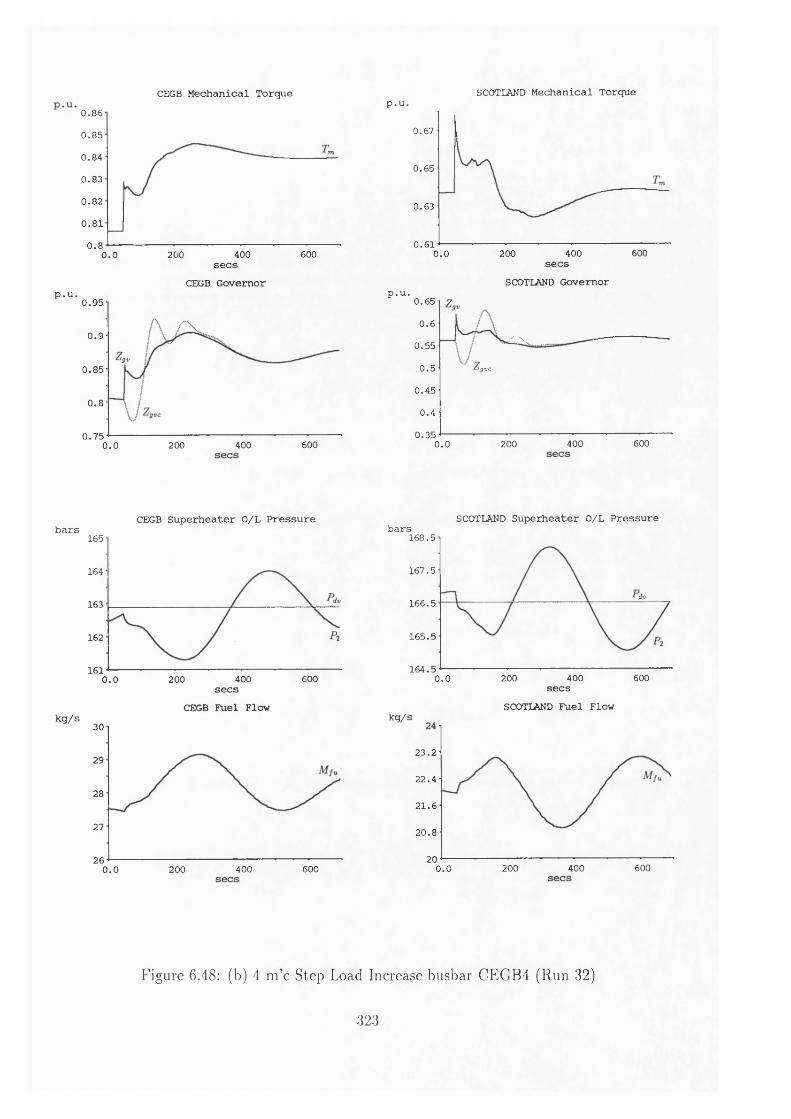
p.u.
bars
kg/s
CEGB Mechanical Torque SCOTLAND Mechanical Torque0.860 .8 5
0 .8 4
0 .8 3
0 .8 2
0 .8 1
0 .86000 .0 200 400
secs CEGB Governor
0 .9 5
0 .9
<g v0 .8 5
0 .8
0 .7 5400 6000.0 200
p.u.
0 .6 7
0 .6 5
0 .6 3
0 .6 1600200 4000.0
secsSCOTLAND Governor
p.u.0 .6 5
0 . 6
ZLV0 .5 5
0 .5 'gvc
0 .4 5
0 .4
0 .3 56004000.0 200
CEGB Superheater O/L Pressure barsSCOTLAND Superheater O/L Pressure
165
164
163
162
161600200 4000.0
secs CEGB Fuel Flow
30
29
28
27
26600200 4000.0
16 8 .5
1 6 7 .5
dv1 66 .5
1 6 5 .5
1 6 4 .56000.0 200 400
secsSCOTLAND Fuel Flow
kg/s
2 3 .2
2 2 .4
21 .6
20.8
20400 6000.0 200
Figure 6.48: (b) 4 m ’c Step Load Increase busbar CEGB4 (Run 32)
323

>1
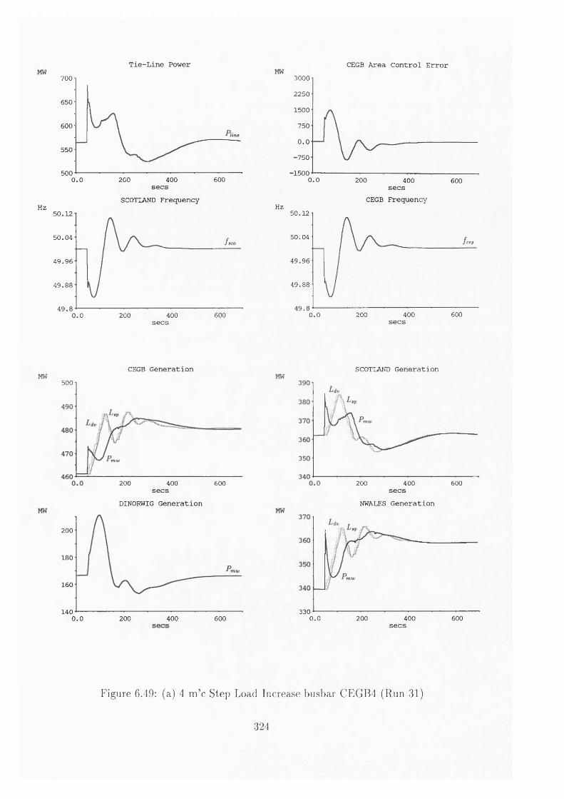
Tie-Line Power CEGB Area Control Error700
650
600
550
500400 6000.0 200
secsSCOTLAND Frequency
Hz5 0 .1 2
5 0 .0 4
4 9 .9 6
4 9 .8 8
4 9 .86000.0 200 400
secs
CEGB Generation500
30002250
1500
750
0.0•750
■15000.0 200 400 600secs CEGB Frequency
Hz50 .1 2
50 .0 4ceg
4 9 .9 6
4 9 .8 8
4 9 .8400 6000.0 200 secs
330 --------------0 .0 200 400 600
secs
SCOTLAND Generation
200 400 600secs
DINORWIG Generation
200 400 600secs
NWALES Generation
200
180
160
1400.0 200 400 600
Figure 6.49: (a) 4 m ’c Step Load Increase busbar CEGB4 (Run 31)
324

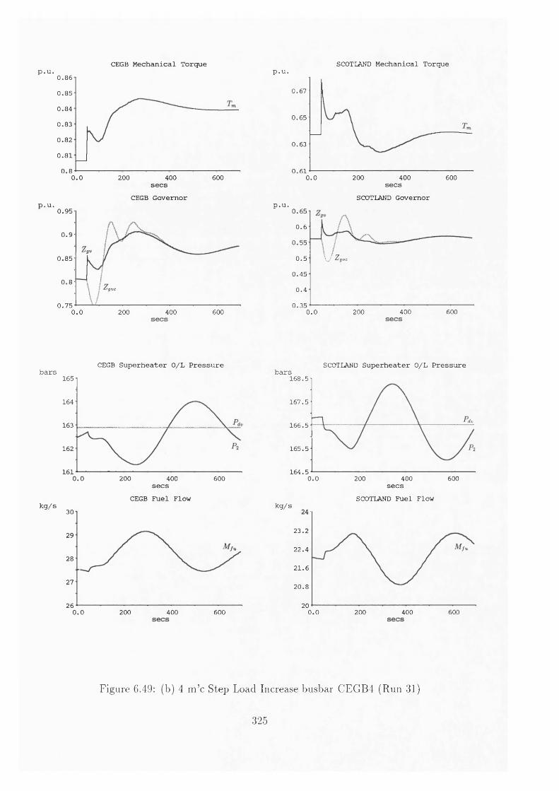
p.u.CEGB Mechanical Torque SCOTLAND Mechanical Torque
p.u.
0.860 .8 5
0 .8 4
0 .8 3
0 .8 2
0 .8 1
0.80.0 200 400 600secs
CEGB Governor0 .9 5
0 .9
0 .8 5
0.8Igvc
0 .7 50.0 200 400 600
p.u.
0 .6 7
0 .6 5
0 .6 3
0 .6 14000.0 200 600
secsSCOTLAND Governor
p.u.0 .6 5
0.60 .5 5
I / Z gvc0 .5
0 .4 5
0 .4
0 .3 5 200 400 6000.0
barsCEGB Superheater O/L Pressure
165
164
163
162
1610.0 200 400 600
kg/s
secs CEGB Fuel Flow
30
29
28
27
260.0 200 400 600
bars SCOTLAND Superheater O/L Pressure16 8 .5
16 7 .5
dv16 6 .5
16 5 .5
164 .50.0 200 400 600
kg/s
secsSCOTLAND Fuel Flow
23 .2
2 2 .4
21.6
20.8
200.0 200 400 600
Figure 6.49: (b) 4 m ’c Step Load Increase busbar CEGB4 (Run 31)
325

U r\
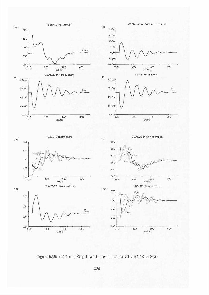
Tie-Line Power CEGB Area Control ErrorMW 700
650
600
550
500200 400 6000.0
Hz
secsSCOTLAND Frequency
5 0 .1 2
5 0 .0 4
4 9 .9 6
4 9 .8 8
4 9 .8200 400 6000.0
MW 30002250
1500
750
0.0■750
-1 5 0 06000.0 200 400
Hz
secs CEGB Frequency
50 .1 2
5 0 .0 4ceg
4 9 .9 6
4 9 .8 8
4 9 .8400 6000.0 200
CEGB Generation SCOTLAND GenerationMW
MW
500
490
480
470
4606000.0 200 400
secsDINOKWIG Generation
200
180
160
140400 6000 . 0 200
MW
MW
390
380
370
360
350
340200 400 6000.0
secsNWALES Generation
370
360
350
340
330200 400 6000.0
secs
Figure 6.50: (a) 4 m ’c Step Load Increase busbar CEGB4 (Run 36a)
326

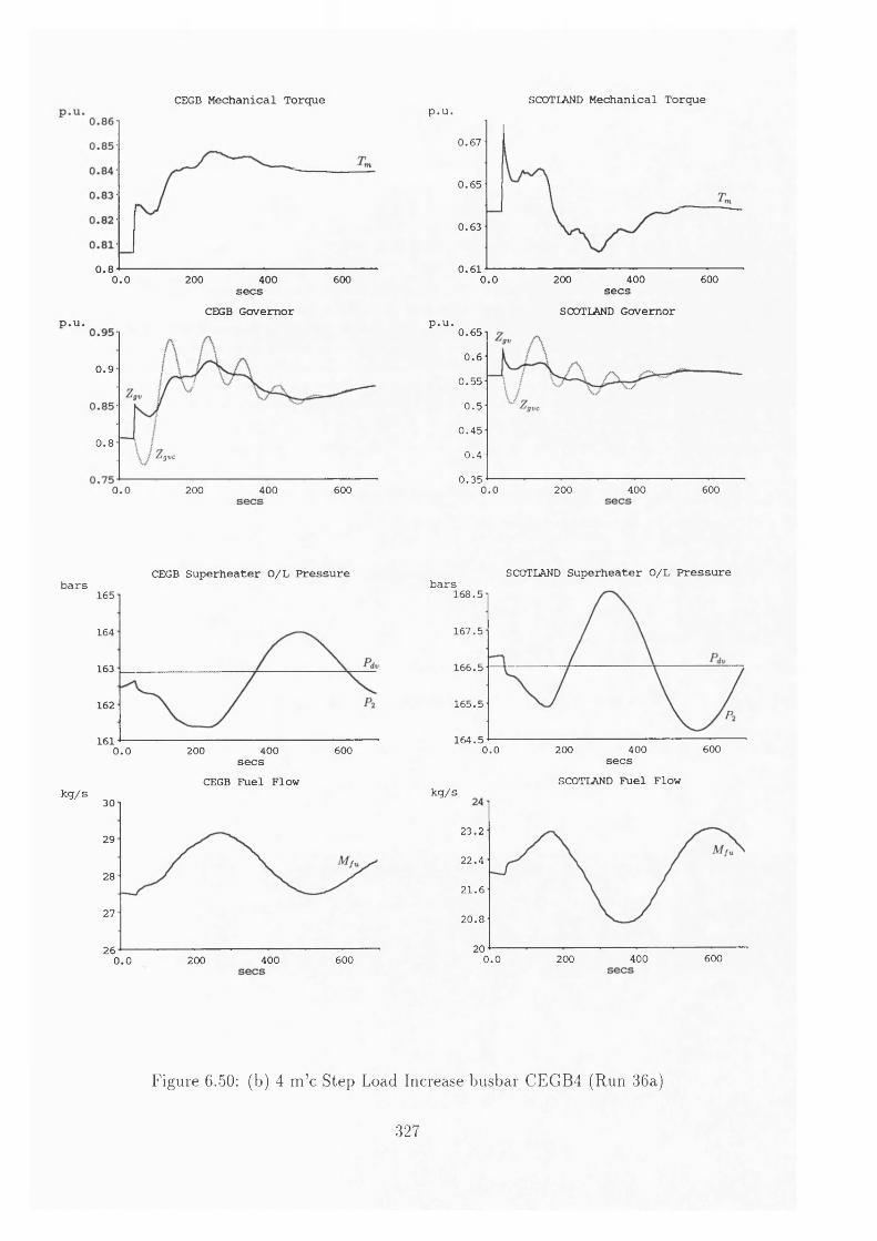
p.u.
bars
kg/s
CEGB Mechanical Torque
0.80.0 200 400 600secs
CEGB Governor
0.9
0.8IgVC
0.0 200 400 600
p.u.SCOTLAND Mechanical Torque
0.67
0.65
0.63
0.610.0 200 400 600secs
SCOTLAND Governorp.u.
0.65
0.60.55
0.5
0.45
0.4
0.350.0 200 400 600
CEGB Superheater O/L Pressure barsSCOTLAND Superheater O/L Pressure
165
164
163
162
161400 6000.0 200
secs CEGB Fuel Flow
30
29
28
27
26400 6000.0 200
168.5
167.5
166.5
165.5
164.56004000.0 200 secs
SCOTLAND Fuel Flowkg/s
23.2
22.4
21.6
20.8
20600200 4000 . 0
Figure 6.50: (b) 4 m ’c Step Load Increase busbar CEGB4 (Run 36a)
327

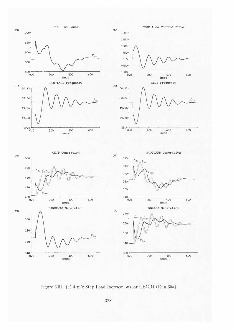
Tie-Line Power CEGB Area Control ErrorMW 700
650
600P lin e
550
5006000.0 200 400
Hz
secsSCOTLAND Frequency
5 0 .1 2
5 0 .0 4
4 9 .9 6
4 9 .8 8
4 9 .80.0 200 400 600
MW 30002250
1500
750
0.0
■750
-1 5 0 00.0 200 400 600
Hz
secs CEGB Frequency
50 .12
50 .04ceg
4 9 .9 6
4 9 .8 8
4 9 .8400 6000.0 200
CEGB Generation SCOTLAND GenerationMW
MW
500
490
480
470
4600.0 200 400 600secs
DINORWIG Generation
200
180
160
1400.0 200 400 600
MW
MW
390
380
370
360
350
3400.0 200 400 600secs
NWALES Generation370
360
350
340
330400 6000.0 200
Figure 6.51: (a) 4 m ’c Step Load Increase busbar CEGB4 (Run 35a)
328

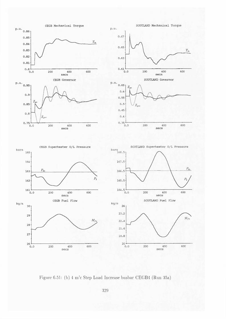
p.u.
bars
kg/s
CEGB Mechanical Torque SCOTLAND Mechanical Torque
0 . 8200 400 6000.0 secs
CEGB Governor
0 .9
0 . 8IgVC
600200 4000.0
p.u.
0 .6 7
0 .6 5
0 .6 3
0 .6 1 200 6000.0 400secs
SCOTLAND Governorp.u.
0 .6 5
0.60 .5 5
0 .5
0 .4 5
0 .4
0 .3 5600200 4000.0
CEGB Superheater O/L Pressure165
164
163
162
1610.0 200 400 600secs
CEGB Fuel Flow30
29
28
26 200 400 6000.0
barsSCOTLAND Superheater O/L Pressure
1 6 8 .5
1 6 7 .5
16 6 .5
1 6 5 .5
16 4 .5400 6000.0 200
secsSCOTLAND Fuel Flow
kg/s
2 3 .2
2 2 .4
2 1 .6
20
20400 6000 . 0 200
secs secs
Figure 6.51: (b) 4 m ’c Step Load Increase busbar CEGB4 (Run 35a)
329

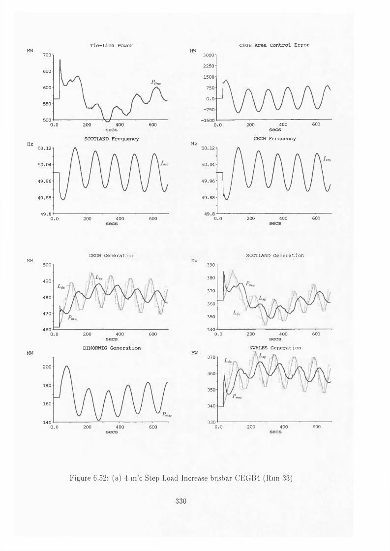
Tie-Line Power CEGB Area Control ErrorMW 700
650
600
550
5000.0 200 400 600
HZ
secsSCOTLAND Frequency
5 0 .1 2
5 0 .0 4
4 9 .9 6
4 9 .8 8
4 9 .8400 6000.0 200
MW 30002250
1500
750
0.0—1■750
■15006004002000.0
HZ
secs CEGB Frequency
50 .12
ceg50 .0 4
4 9 .9 6
49 .8 8
200 400 6000.0
CEGB Generation SCOTLAND GenerationMW
MW
500
490
480
470
4600.0 400200 600secs
DINORWIG Generation
200
180
160
140400 6000.0 200
MW
MW
390
380
370
360
350
3406000.0 200 400
secsNWALES Generation
370
360
350
340
330 6000.0 200 400
Figure 6.52: (a) 4 m ’c Step Load Increase busbar CEGB4 (Run 33)
330

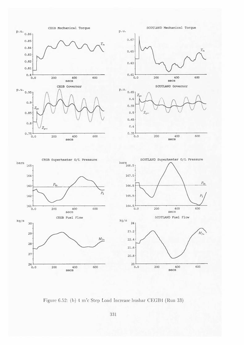
p.u.
bars
kg/s
CEGB Mechanical Torque SCOTLAND Mechanical Torque0.860 .8 5
0 .8 4
0 .8 3
0 .8 2
0 .8 1
0.8400 6000.0 200
secs CEGB Governor
0 .9 5
0 .9
0 .8 5
0.8'J V C
0 .7 5600200 4000.0
p.u.
0 .6 7
0 .6 5
0 .6 3
0 .6 1400 6000.0 200
secsSCOTLAND Governor
p.u.0 .6 5
A0.60 .5 5
\ J0 .5 igvc
0 .4 5
0 .4
0 .3 5400 6000.0 200
CEGB Superheater O/L Pressure SCOTLAND Superheater O/L Pressure165
164
163
162
161 200 400 6000.0secs
CEGB Fuel Flow30
29
28
27
266000.0 200 400
bars1 6 8 .5
1 6 7 .5
1 6 6 .5
1 6 5 .5
1 6 4 .5400 6000.0 200
secsSCOTLAND Fuel Flow
kg/s
2 3 .2
2 2 .4
21.6
20.8
20400 6002000.0
Figure 6.52: (b) 4 m ’c Step Load Increase busbar CEGB4 (Run 33)
331

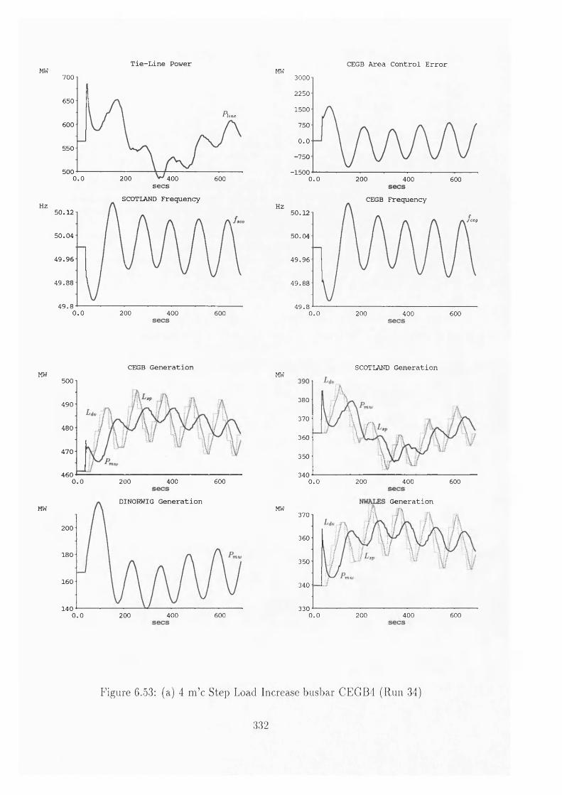
Tie-Line Power CEGB Area Control ErrorMW MW700
650
P lin e
600
550
5000.0 200 400 600secs
SCOTLAND FrequencyHz5 0 .1 2
5 0 .0 4
4 9 .9 6
4 9 .8 8
4 9 .80.0 200 400 600
30002250
1500
750
0.0■750
-15000.0 200 400 600
CEGB FrequencyHz50 .1 2
'ceg
50 .0 4
49 .9 6
49 .8 8
4 9 .80.0 200 400 600
CEGB Generation SCOTLAND GenerationMW500
490
480
470
4600.0 200 400 600
MW
380
370
360
350
3400.0 200 400 600
MW DINORWIG Generation
200
180
160
1400.0 200 400 600
MWGeneration
370
360
350
340
3300.0 200 400 600
Figure 6.53: (a) 4 m ’c Step Load Increase busbar CEGB4 (Run 34)
332

7J-{ £
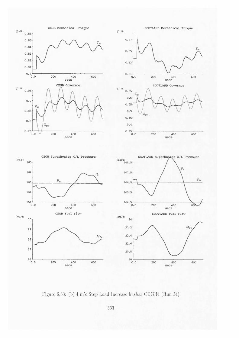
p.u.
bars
kg/s
CEGB Mechanical Torque
0.80.0 200 400 600secs
CEGB Governor
0 .9
0.8
0.0 200 400 600secs
p.u. SCOTLAND Mechanical Torque
0 .6 7
0 .6 5
0 .6 3
0 .6 10.0 200 400 600secs
SCOTLAND Governorp.u.0 .6 5
0.60 .5 5
0 .5
0 .4 5
0 .4
0 .3 50.0 200 400 600
CEGB Superheater O/L Pressure165
164
163
162
1610.0 200 400 600secs
CEGB Fuel Flow30
29
28
27
260.0 200 400 600
SCOTLAND Superheater O/L Pressurebars168 .5
167 .5
166 .5
165 .5
164 .50.0 200 400secs
kg/sSCOTLAND Fuel Flow
23 .2
2 2 .4
21.6
20.8
200.0 200 400 600
Figure 6.53: (b) 4 m ’c Step Load Increase busbar CEGB4 (Run 34)
333

k i f ©
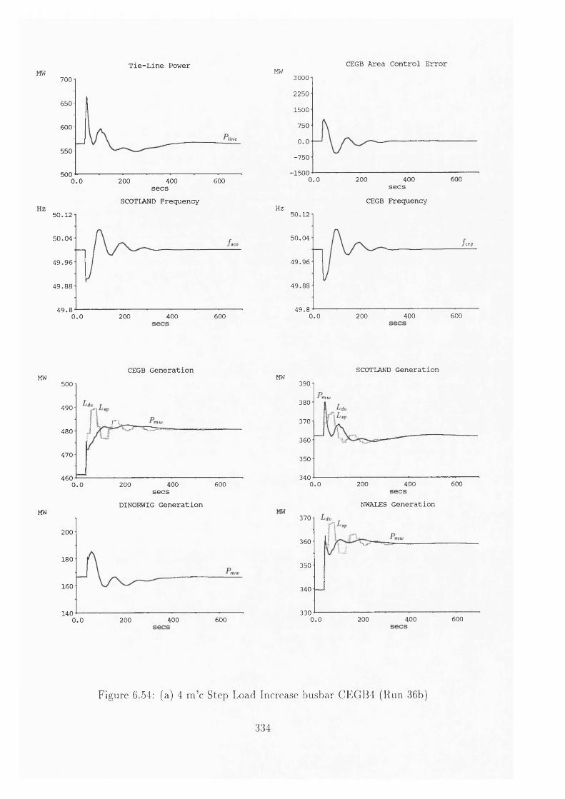
Tie-Line PowerMW 700
650
600line
550
500 200 400 6000.0secs
SCOTLAND Frequency5 0 .1 2
5 0 .0 4
4 9 .9 6
4 9 .8 8
4 9 .8 200 400 6000.0
CEGB Area Control ErrorMW 3000
2250
1500
750
0.0-7 5 0
■1500 200 400 6000.0secs
CEGB FrequencyHz
50 .12
50 .04ceg
49 .9 6
49 .8 8
4 9 .86000.0 200 400
CEGB GenerationMW
500
490
rv480
470
4600.0 200 400 600secs
DINORWIG GenerationMW
200
180
160
140400 6000.0 200
SCOTLAND GenerationMW
390
380
370
360
350
3400 .0 200 400 600
secsNWALES Generation
370
360
350
340
330400 6000.0 200
Figure 6.54: (a) 4 m ’c Step Load Increase busbar CEGB4 (Run 36b)
334

k , S it- (cC)
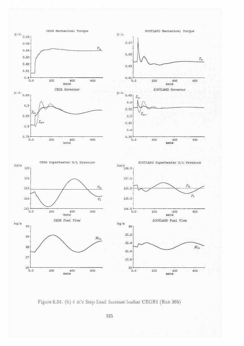
p.u.
bars
kg/s
CEGB Mechanical Torque0.860 .8 5
0 .8 4
0 .8 3
0 .8 2
0 .8 1
0.80.0 200 400 600secs
CEGB Governor0 .9 5
0 .9
0 .8 5
0.8
0 .7 50.0 200 400 600secs
SCOTLAND Mechanical Torquep.u.
0 .6 7
0 .6 5
0 .6 3
0 .6 10.0 400200 600
secsSCOTLAND Governor
p.u. u.co'gv
0.6
0 .5 5
'gvc0 .5
0 .4 5
0 .4
0 .3 50.0 200 400 600
CEGB Superheater O/L Pressure165
164
163
162
1610 .0 200 400 600
secs CEGB Fuel Flow
30
29
28
27
260.0 200 400 600
SCOTLAND Superheater O/L Pressurebars168 .5
167 .5
16 6 .5
165 .5
164 .50.0 200 400 600
secsSCOTLAND Fuel Flowkg/s
23 .2
2 2 .4
21.6
20.8
200.0 200 400 600
Figure 6.54: (b) 4 m ’c Step Load Increase busbar CEGB4 (Run 36b)
335
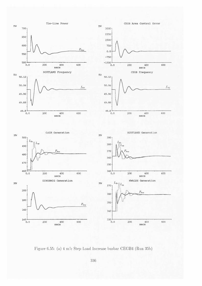
Tie-Line Power CEGB Area Control ErrorMW MW700
650
600
550
5000.0 200 400 600
Hz
secsSCOTLAND Frequency
5 0 .1 2
5 0 .0 4
4 9 .9 6
4 9 .8 8
4 9 .80.0 200 400 600
30002250
1500
750
0 . 0 —
-7 5 0
■15000.0 200 400 600
Hz
secs CEGB Frequency
50 .12
50 .04ceg
49 .9 6
49 .88
49 .80 .0 600200 400
CEGB Generation SCOTLAND GenerationMW
MW
500
490
480
470
4600.0 200 400 600secs
DINORWIG Generation
200
180
160
1400.0 200 400 600
MW
MW
390
380
370
360
350
340 200 400 6000.0secs
NWALES Generation370
360
350
340
330200 400 6000.0
Figure 6.55: (a) 4 m ’c Step Load Increase busbar CEGB4 (Run 35b)
336


p.u.
bars
kg/s
CEGB Mechanical Torque0.86
0 .8 5
0.80.0 200 400 600secs
CEGB Governor
0 .9
0.8fgvc
0.0 200 400 600
p.u.SCOTLAND Mechanical Torque
0 .6 7
0 .6 5
0 .6 3
0 .6 10.0 200 400 600secs
SCOTLAND Governorp.u.
0 .6 5
0.6
0 .5 5
0 .5
0 .4 5
0 .4
0 .3 50.0 200 400 600
CEGB Superheater O/L Pressurebars SCOTLAND Superheater O/L Pressure
165
164
163
162
161200 4000.0 600
secs CEGB Fuel Flow
30
29
28
27
260.0 200 400 600
16 8 .5
1 6 7 .5
16 6 .5
1 6 5 .5
164 .50.0 400 600200secs
SCOTLAND Fuel Flowkg/s
2 3 .2
2 2 .4
21 .6
20.8
200.0 200 400 600
Figure 6.55: (b) 4 m ’c Step Load Increase busbar CEGB4 (Run 35b)
337

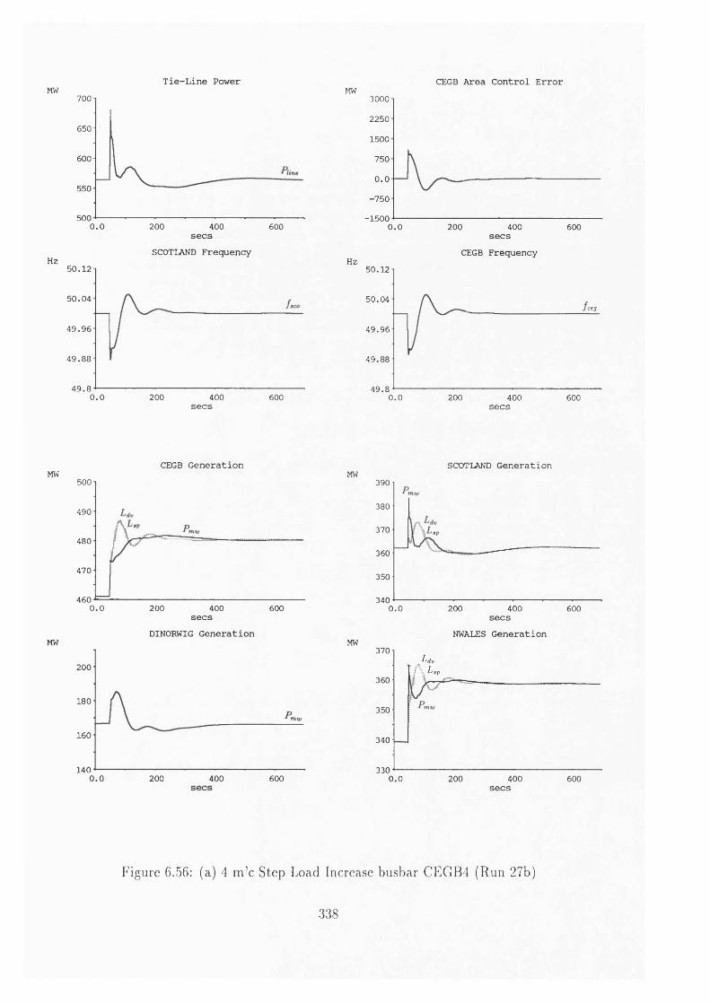
Tie-Line PowerMW 700
650
600
550
5000.0 200 400 600secs
SCOTLAND Frequency Hz5 0 .1 2
5 0 .0 4
4 9 .9 6
4 9 .8 8
4 9 .80.0 400200 600secs
CEGB Area Control ErrorMW 3000
2250
1500
750
0.0•750
-15 0 00.0 200 400 600secs
CEGB FrequencyHz
5 0 .12
5 0 .04ceg
4 9 .9 6
49
4 9 .80.0 200 400 600
secs
CEGB GenerationMW
MW
500
490
480
470
4600.0 200 400 600secs
DINORWIG Generation
200
180
160
1400 . 0 200 400 600
MW
MW
SCOTLAND Generation390
380
370 '*p
360
350
3400.0 200 400 600
secsNWALES Generation
370
360
350
340
330
Ldvi \ L’v
0.0 200 400secs
600
Figure 6.56: (a) 4 m ’c Step Load Increase busbar CEGB4 (Run 27b)
338

1 ? lo V o <o •
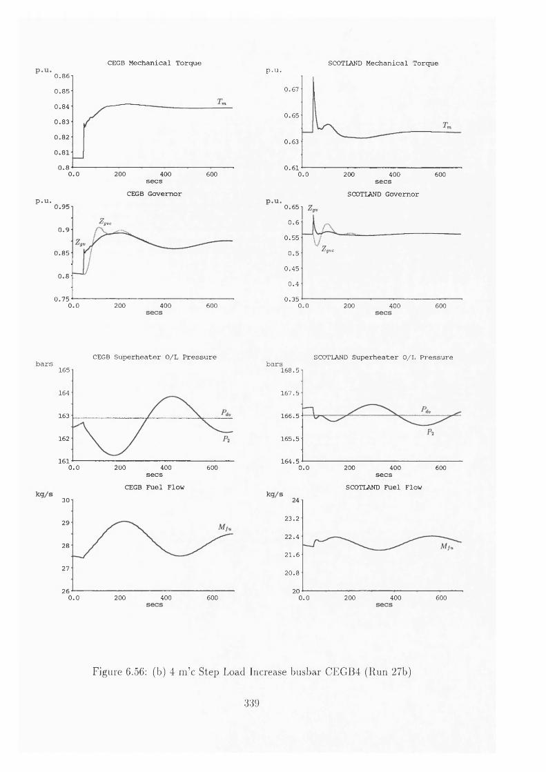
CEGB Mechanical Torque0.860 .8 5
0 .8 4
0 .8 3
0 .8 2
0 .8 1
0.80.0 200 400 600secs
CEGB Governorp.u . u.yo
'gvc0 .9
0 .8 5
0 .8
0 .7 50.0 200 400 600
SCOTLAND Mechanical Torquep.u.
0 .6 7
0 .6 5
0 .6 3
0 .6 10.0 200 400 600secs
SCOTLAND Governor0 .6 5
0 . 6
0 .5 5
igvc0 .5
0 .4 5
0 .4
0 .3 50.0 200 400 600
CEGB Superheater O/L Pressurebars
165
164
163
162
1610 .0 200 400 600
secs CEGB Fuel Flow
30
29
28
27
260.0 200 400 600
SCOTLAND Superheater O/L Pressurebars16 8 .5
16 7 .5
16 6 .5
16 5 .5
1 6 4 .50.0 200 400 600
secsSCOTLAND Fuel Flow
2 3 .2
2 2 .4
2 1 .6
20.8
200.0 200 400 600
Figure 6.56: (b) 4 m ’c Step Load Increase busbar CEGB4 (Run 27b)
339

V - h
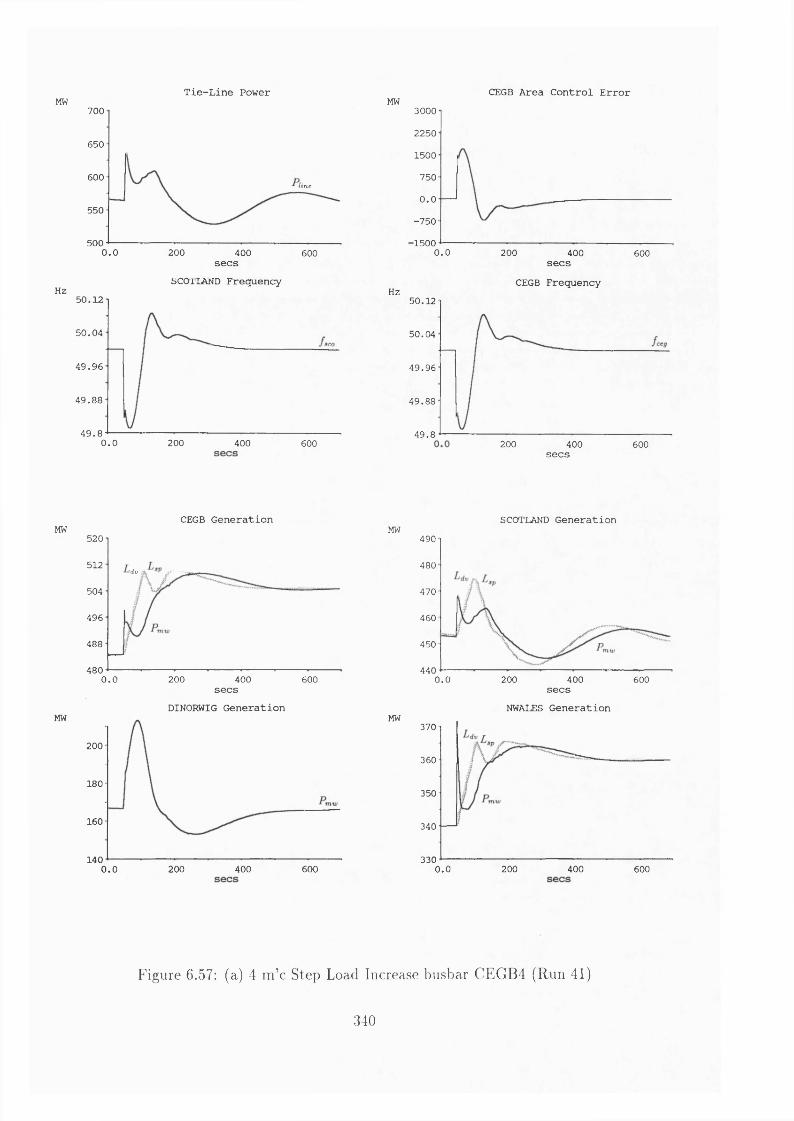
Tie-Line PowerMW 700
650
600line
550
5000.0 200 400 600
Hz
secsSCOTLAND Frequency
5 0 .1 2
5 0 .0 4
4 9 .9 6
4 9 .8 8
4 9 .80.0 200 400 600
MW
Hz50 .12
CEGB Area Control Error30002250
1500
750
0.0-7 5 0
•15000.0 200 400 600secs
CEGB Frequency
600
50 .04
4 9 .9 6
4 9 .8 8
4 9 .8200 400
secs
CEGB Generation MW
520
512'dv
504
496
488
4800.0 200 400 600secs
DINORWIG GenerationMW
200
180
160
1400.0 200 400 600
SCOTLAND Generation MW490
480
470
460
450
4400 .0 200 400 600
secs NWALES Generation
MW370
360
350
340
3300 .0 200 400 600
Figure 6.57: (a) 4 m ’c Step Load Increase busbar CEGB4 (Run 41)
340

4 7 ^
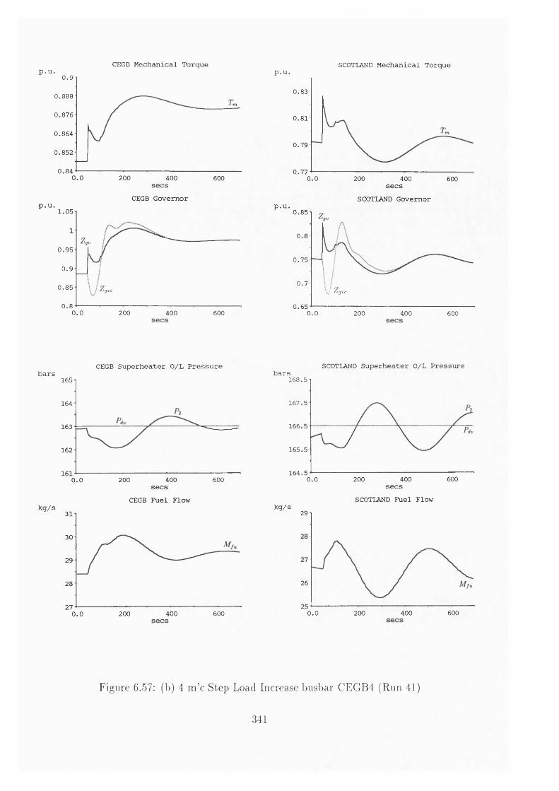
p.u. CEGB Mechanical Torque
p.u.
0.9
0.888
0 .8 7 6
0 .8 6 4
0 .8 5 2
0 .8 40.0 200 400 600secs
CEGB Governor1 .0 5
IgV0 .9 5
0 .9
0 .8 5 igvc
0.80.0 200 400 600
p.U. SCOTLAND Mechanical Torque
0 .8 3
0 .8 1
0 .7 9
0 .7 70.0 200 400 600secsSCOTLAND Governor
p.u.0 .8 5
0.8
0 .7 5
0 .7V Zs„c
0 .6 50.0 200 400 600
barsCEGB Superheater O/L Pressure
165
164
163
162
161 200 400 6000.0
kg/s
secs CEGB Fuel Flow
31
30
29
28
27400 6000.0 200
barsSCOTLAND Superheater O/L Pressure
1 68 .5
1 67 .5
1 6 6 .5
165 .5
16 4 .5400 6000.0 200
kg/s
secsSCOTLAND Fuel Flow
29
26
25 200 400 6000.0
Figure 6.57: (b) 4 m ’c Step Load Increase busbar CEGB4 (Run 41)
341

4 1 4 -1-0 (
*
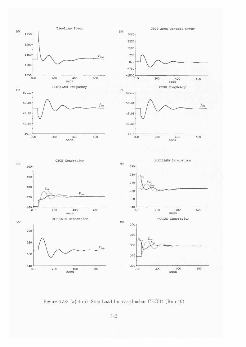
Tie-Line Power1250
1200
1150
1100
10500.0 200 400 600secs
SCOTLAND FrequencyHz
5 0 .1 2
5 0 .0 4
4 9 .9 6
4 9 .8 8
4 9 .80.0 200 400 600
CEGB Area Control ErrorMW3000
2250
1500
750
0.0-7 5 0
-1 5 0 00.0 200 400 600secs CEGB Frequency
Hz50 .12
50 .04
4 9 .9 6
49
4 9 .80.0 200 400 600
CEGB GenerationMW
500
490
480
470
460400 6000.0 200
secsDINOKWIG Generation
MW
200
180
160
140400 6000.0 200
SCOTLAND GenerationMW
390
380
370
360
350
3406000.0 200 400
secsNWALES Generation
MW370
360
/ \ L ,350
340
330400 6000.0 200
Figure 6.58: (a) 4 m ’c Step Load Increase busbar CEGB4 (Run 40)
342

t r .O '& C W )
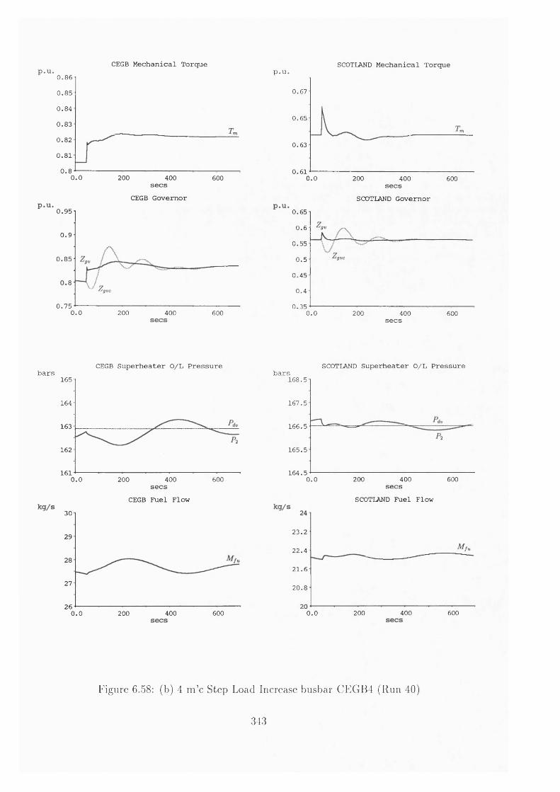
CEGB Mechanical Torque0.860 .8 5
0 .8 4
0 .8 3
0 .8 2
0 .8 1
0.80.0 200 400 600secs
CEGB Governor0 .9 5
0 .9
0 .8 5
8
0 .7 50.0 200 400 600
SCOTLAND Mechanical Torquep.u.
0 .6 7
0 .6 5
0 .6 3
0 .6 10.0 200 400 600secs
SCOTLAND Governor0 .6 5
0.60 .5 5
0 .5
0 .4 5
0 .4
0 .3 50.0 200 400 600secs
CEGB Superheater O/L Pressurebars
165
164
163
162
1610.0 200 400 600secs
CEGB Fuel Flow30
29
28
27
260.0 200 400 600
SCOTLAND Superheater O/L Pressurebars
168 .5
1 6 7 .5
16 6 .5
1 65 .5
1 6 4 .50 .0 200 400 600
secsSCOTLAND Fuel Flow
2 3 .2
2 2 .4
21.6
20.8
200.0 200 400 600
Figure 6.58: (b) 4 m ’c Step Load Increase busbar CEGB4 (Run 40)
343

^ ^ (p ( b )
Tie-Line PowerMW
MW
600
400
200
0.0P i,
MW
0.0 20 40 60 80secs
DINORWIG1 Generation
100
-285•290-295■300■305■310-315
10020 40 60 800.0secs
LONGANNET Generation
600
500
400
300
200 20 60 80 1000.0 40
HZFrequency
MW
MW
51.2
50.8
50.4
50 ceg
49.60.0 60 80 10020 40secs
DINORWIG2 Generation-285-290■295■300■305■310■315 60 80 100400.0 20 secs
DRAX.B Generation695
685
675
665
655 60 80 1000.0 20 40
Figure 7.1: (a) 25 m ’c Scotland-England Split (Run 1)
344
COTTAM Generation RATCLIFFE GenerationMW
MW
370
360
350
340
330
32010060 800.0 20 40
secsEGGBORO. Generation
490
480
470
460
450
440 1000.0 20 40 60 80
MW
MW
380
370
360
350 ' s p
340
33010040 60 800.0 20 secs
RUGELEY Generation520
512
504
496
488
48010020 40 60 800.0
HUNTERSTN. Generation HINKLEY GenerationMW
MW
375
350
325
300
275
250
22560 80 1000.0 20 40
secsPETERHEAD Generation
630
610
590
570
550
5300.0 20 40 60 80 100
MW
MW
440
435
430
425
420
415
410 10020 40 60 800.0secs
HEYSHAM Generation
700
680
660
6400.0 20 40 60 80 100
Figure 7.1: (b) 25 m ’c Scotland-England Split (Run 1)
345
LONGANNET Mechanical Torquep.u.
0 .7
0.6
0 .5
0 .4
0 .30.0 40 60 80 10020
p.u
secsCOTTAM Mechanical Torque
0 .7
C .675
0 .6 5
0 .6 2 5
0.60 .5 7 5
0 .5 50.0 40 60 80 10020
p.u.DRAX.B Mechanical Torque
p.u.
0.950 .9 2 5
0 .9
0 .8 7 5
0 .8 5
0 .8 2 5
0.840 60 80 1000.0 20
secsRATCLIFFE Mechanical Torque
0 .7
0 .6 7 5
0 .6 5
0 .6 2 5
0.60 .5 7 5
0 .5 540 60 80 1000.0 20 secs
p.u. EGGBORO. Mechanical Torque
p.u.
0 .9
0 .8 7 5
0 .8 5
0 .8 2 5
0.80 .7 7 5
0 .7 50.0 20 40 60 80 100secs
HUNTERSTN. Mechanical Torque0 .5
0 .4 6
0 .4 2
0 .3 8
0 .3 40.0 20 40 60 80 100
p.u.RUGELEY Mechanical Torque
0 .8 7 5
0 .8 5
0 .8 2 5
0.80 .7 7 5
0 .7 50.0 20 40 60 80 100
p.u.
secsHINKLEY Mechanical Torque
0 .6 5
0 .6 2 5
0.6
0 .5 7 5
0 .5 5
0 .5 2 5
0 .50.0 20 40 60 80 100
Figure 7.1: (c) 25 m ’c Scotland-England Split (Run 1)
346
LONGANNET Governor DRAX.B Governorp.u.
1.1
0 .9
0 .7
0 .5
0 .380 10040 600.0 20 secs
COTTAM Governorp.u.
0 .7
0 .6 5
0.6'gvc
0 .5 5
0 .5
0 .4 5
0 .460 80 1000.0 20 40
p.u. 1.2
1.12
1 .0 4
0 .9 6
0.88 10040 60 800.0 20secs
RATCLIFFE Governorp.u.
0 .7IgV
0 .6 5
0.6 'gvc
0 .5 5
0 .5
0 .4 5
0 .4 20 40 60 80 1000.0
EGGBORO. Governor RUGELEY Governorp.u. 1.12
1 .0 4
‘gvc0 .9 6
0.88
1000.0 20 40 60 80
p.U.
secsHUNTERSTN. Governor
0 .6 5
0.60 .5 5 'gvc
0 .5
0 .4 5
0 .4
0 .3 50.0 20 40 60 80 100
p.u. 1.21 .1 5
1.11 .0 5 ‘gvc
0 .9 5
0 .960 80 1000.0 20 40
p.u.
secsHINKLEY Governor
0 .6 5
0.60 .5 5
I gV
0 .5‘gvc
0 .4 5
0 .4
0 .3 5 600.0 20 40 80 100
Figure 7.1: (d) 25 m ’c Scotland-England Split (Run 1)
347
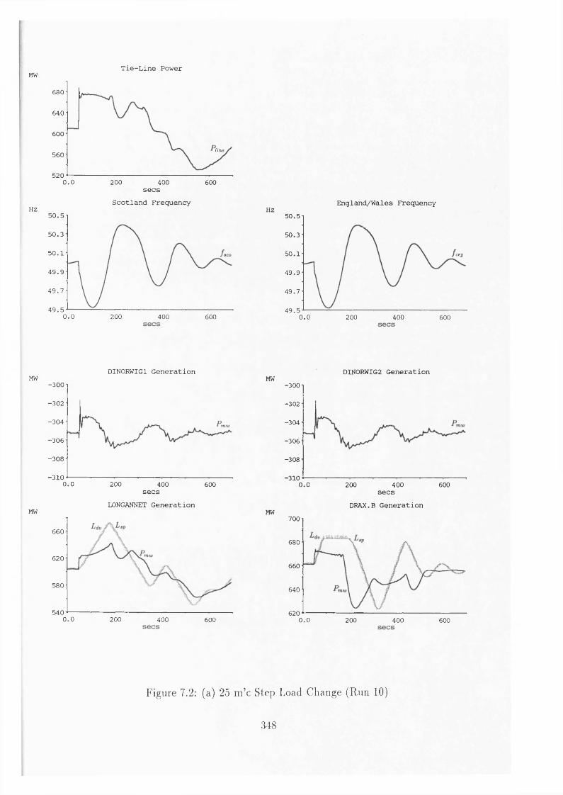
Tie-Line PowerMW
Hz
680
640
600Imi560
5200.0 200 400 600secs
Scotland Frequency50.5
50.3
50.1
49.9
49.7
49.50.0 200 400 600
HZEngland/Wales Frequency
50.5
50.3
50.1 ceg
49.9
49.7
49.50.0 200 400 600
DINORWIG1 GenerationMW DIN0RWIG2 Generation
MW
-300
-302
-304
■306
-308
-3100.0 200 400 600secs
L0NGANNET Generation
660
620
580
5400.0 200 400 600
MW
MW
-300
-302
-304
•306
-308
■3100.0 200 400 600secs
DRAX.B Generation700
680
660
640
6200.0 200 400 600
Figure 7.2: (a) 25 m ’c Step Load Change (Run 10)
348

(O
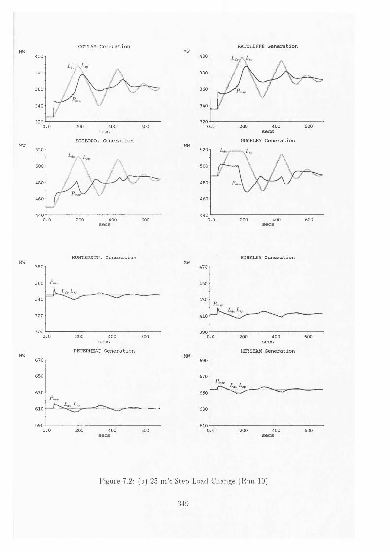
COTTAM Generation RATCLIFFE GenerationMW
MW
400'dv j\~ sp
380
360
340
3200.0 200 400 600secs
EGGBORO. Generation520
500
480
460
4400.0 200 400 600
MW
MW
400
380
360
340
3206000.0 200 400
secsRUGELEY Generation
520
500
480
460
4400.0 200 400 600
HUNTERSTN. Generation HINKLEY GenerationMW
MW
380
360
340
320
3000.0 200 400 600secs
PETERHEAD Generation670
650
630
610
5900.0 200 400 600
MW
MW
470
450
430
410
3900.0 200 400 600secs
HEYSHAM Generation690
670
650
630
6100.0 200 400 600
Figure 7.2: (b) 25 m ’c Step Load Change (Run 10)
349

■o
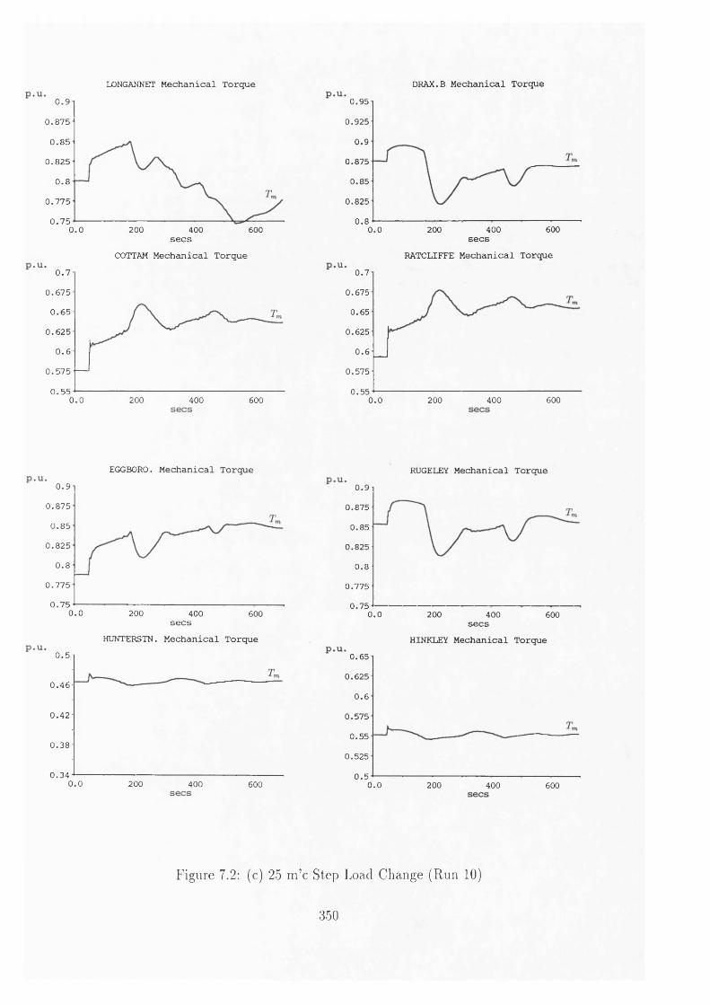
LONGANNET Mechanical Torque0.9
0 .8 7 5
0 .8 5
0 .8 2 5
0.80 .7 7 5
0 .7 50.0 200 400 600secs
COTTAM Mechanical Torque0 .7
0 .6 7 5
0 .6 5
0 .6 2 5
0.60 .5 7 5
0 .5 50.0 200 400 600
DRAX.B Mechanical Torque0.95
0 .925
0 .9
0 .8 7 5
0 .8 5
0 .8 2 5
0 .86000 .0 200 400
secsRATCLIFFE Mechanical Torque
0 .7
0 .6 7 5
0 .6 5
0 .6 2 5
0 . 6
0 .5 7 5
0 .5 50.0 400 600200
EGGBORO. Mechanical Torque0 .9
0 .8 7 5
0 .8 5
0 .8 2 5
0.80 .7 7 5
0 .7 50.0 200 400 600
secsHUNTERSTN. Mechanical Torque
0 .5
0 .4 6
0 .4 2
0 .3 8
0 .3 40.0 200 400 600
RUGELEY Mechanical Torque0 .9
0 .8 7 5
0 .8 5
0 .8 2 5
0 . 8
0 .7 7 5
0 .7 50.0 200 400 600secs
HINKLEY Mechanical Torque0 .6 5
0 .6 2 5
0 .6
0 .5 7 5
0 .5 5
0 .5 2 5
0 .50.0 200 400 600
Figure 7.2: (c) 25 m ’c Step Load Change (Run 10)
350

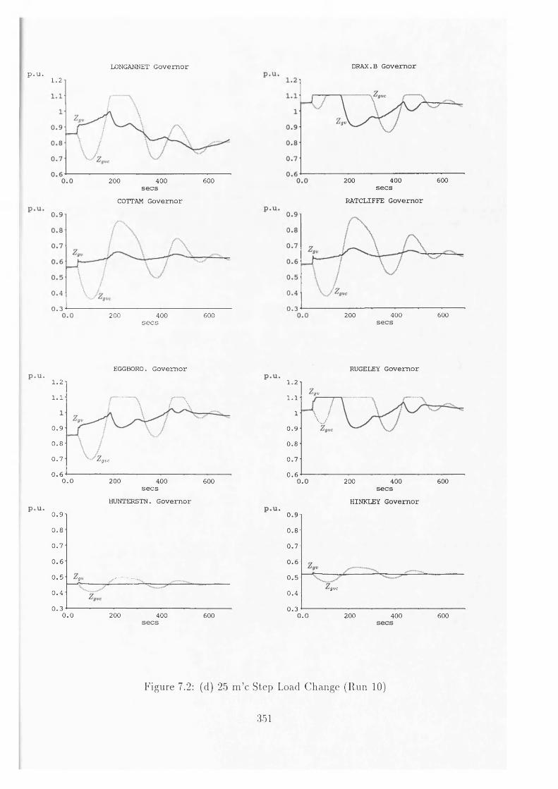
LONGANNET Governorp.u. 1.2
200 400 600s e c s
200 400 600secs
COTTAM Governor
DRAX.B Governor
200 400 600se c s
200 400 600secs
RATCLIFFE Governor
EGGBORO. Governor1.21.1 x/ \
0 .9
0.80 .7 ' g v c
0 . 60.0 200 400 600secs
HUNTERSTN. Governor0 .9
0.80 .7
0.60 .5 i g v
0 .4
0 .30.0 200 400 600
RUGELEY Governor1.2
I g v1.1
1V
0 .9
0.80 .7
0.60.0 200 400 600secs
HINKLEY Governor0 .9
0.80 .7
0.60 .5
'gvc0 .4
0 .30.0 200 400 600
Figure 7.2: (d) 25 m ’c Step Load Change (Run 10)
351

U
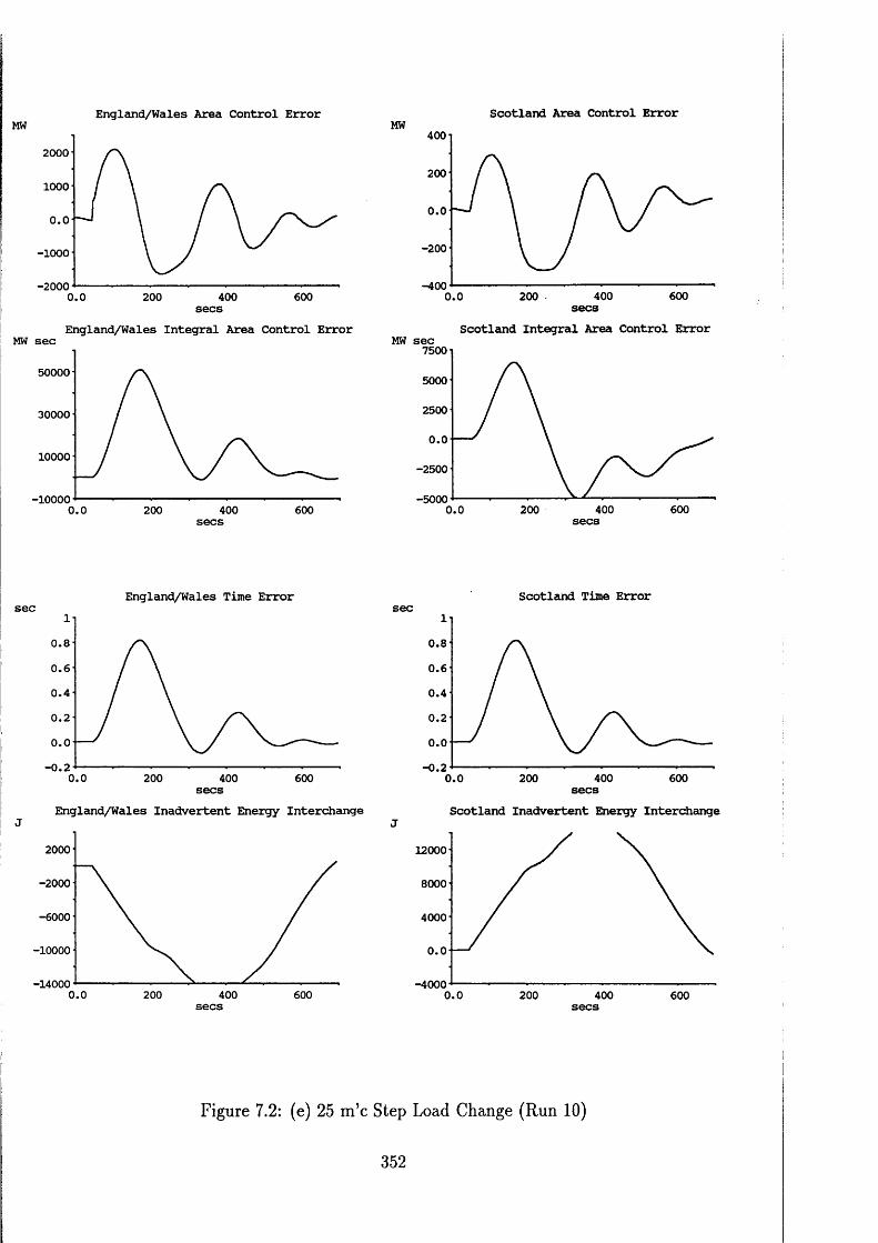
England/Wales Area Control ErrorMW2000
1000
0.0
-1000
-2000400 6000.0 200 secs
England/Wales Integral Area Control ErrorMW sec
50000
30000
10000
-100000.0 400 600200
Scotland Area Control ErrorMW 400
200
0.0
-200
-4006004002000.0 secs
Scotland Integral Area Control ErrorMW sec
7500
5000
2500
0.0
-2500
6004000.0 200
England/Wales Time Errorsec
0.80.60 .4
0.20.0
-0.20.0 200 400 600secs
England/Wales Inadvertent Energy InterchangeJ
2000
-2000
-6000
-10000
-140000 .0 400 600200
Scotland Time Errorsec
0.80.60 .4
0.20.0
-0.24000.0 200 600secs
Scotland Inadvertent Energy InterchangeJ
12000
8000
4000
0.0
-40000.0 200 400 600
Figure 7.2: (e) 25 m ’c Step Load Change (Run 10)
352

t o
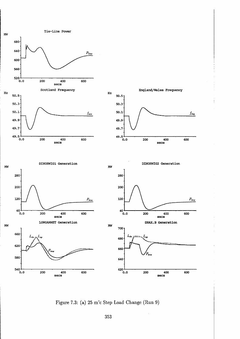
Tie-Line PowerMW
HZ
680
640
600
560
5200.0 200 400 600secsScotland Frequency
50.5
50.3
50.1
49.9
49.7
49.50.0 200 400 600
Hz England/Wales Frequency50.5
50.3
50.1
49.9
49.7
49.50.0 200 400 600
DIN0RWIG1 Generation DINORWIG2 GenerationMW
280
200
120
400.0 200 400 600
MW
secsLONGANNET Generation
660
620
580
5400.0 200 400 600
MW
MW
280
200
120
400.0 200 400 600secs
DRAX.B Generation700
680
660
640
6200.0 200 400 600secs
Figure 7.3: (a) 25 m ’c Step Load Change (Run 9)
353

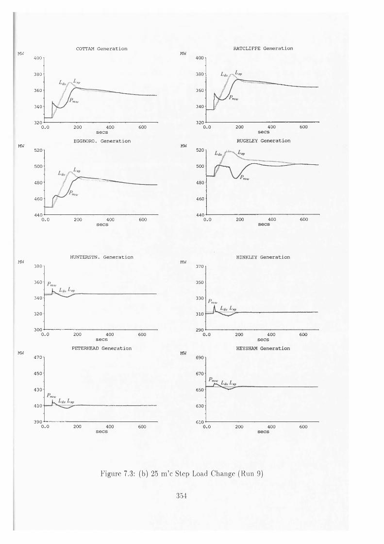
COTTAM Generation RATCLIFFE GenerationMW
MW
secsEGGBORO. Generation
MW400
380
' ap
360
340
3200.0 200 400 600
MW520
500
480
460
4400.0 200 400 600
380
360
340
320400 6000.0 200
secsRUGELEY Generation
520
500
480
460
440400 6000.0 200
HUNTERSTN. Generation HINKLEY GenerationMW
MW
secsPETERHEAD Generation
MW380
360
340
320
3000.0 200 400 600
MW470
450
430
410
3900.0 200 400 600
370
350
330
310
2900.0 200 400 600secs
HEYSHAM Generation690
670
650
630
6100.0 200 400 600
Figure 7.3: (b) 25 m ’c Step Load Change (Run 9)
354

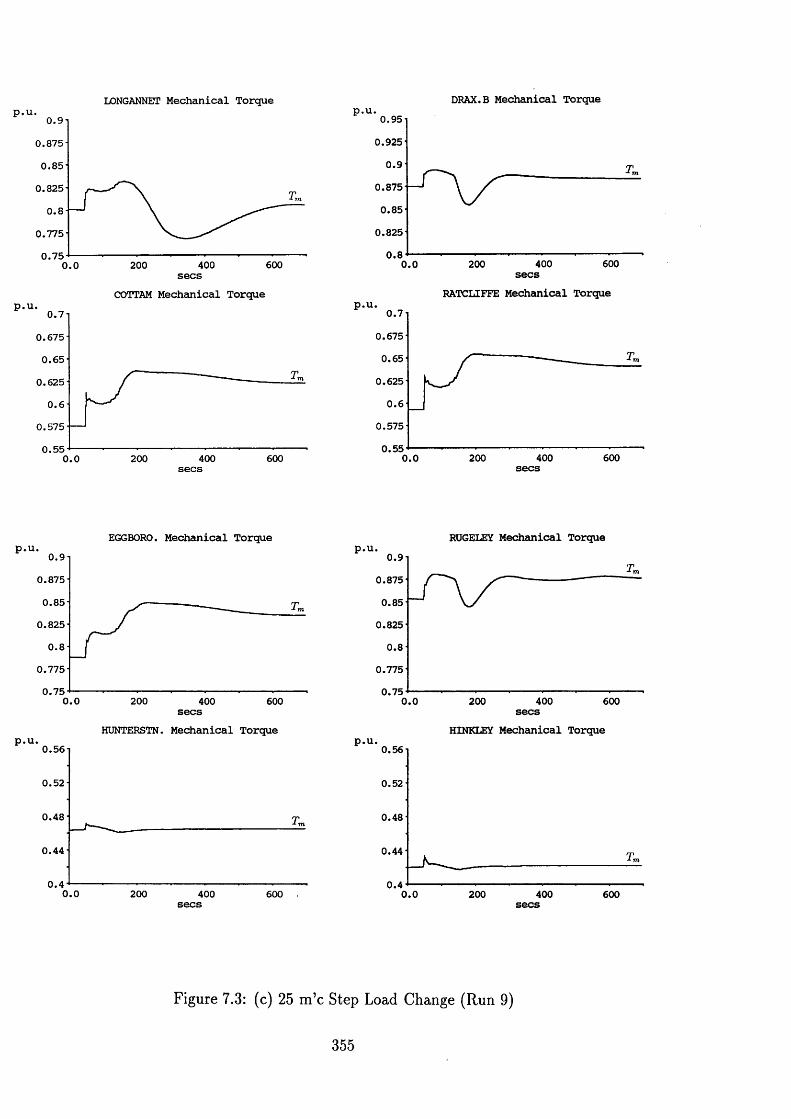
LONGANNET Mechanical Torque DRAX.B Mechanical Torque0.9
0.875
0 .8 5
0 .825
0 . 8
0.775
0 .7 56004002000 .0 secs
COTTAM Mechanical Torque0 .7
0 .675
0 .6 5
0 .625
0.60 .575
0 .5 5200 400 6000.0
0.950 .925
0 .9
0 .875
0 .8 5
0 .825
0.86004002000.0 secs
RATCLIFFE Mechanical Torque0 .7
0.675
0 .65
0.625
0 .6
0.575
0 .5 5600200 4000.0
EGGBORO. Mechanical Torque0 .9
0.875
0 .8 5
0.825
0.80.775
0 .7 50.0 200 600400secs
HUNTERSTN. Mechanical Torque0 .5 6
0 .52
0 .4 8
0 .44
0 .40.0 200 400 600
RUGELEY Mechanical Torque0 .9
0.875
0.85
0.825
0.80.775
0.754000.0 200 600
secs HINKLEY Mechanical Torque
0.56
0.52
0.48
0.44
0 .4 4000.0 200 600
Figure 7.3: (c) 25 m ’c Step Load Change (Run 9)
355

LONGANNET Governor1.21.1
0 .9
0.80 .7
0.60.0 200 400 600
secsCOTTAM Governor
0 .9
0.80 .7
0 . 6
0 .5
0 .4 'gvc
0 .30.0 200 400 600
DRAX.B Governor1.21.1
1 'JV C
0 .9
0 . 8
0 .7
0.6 2000.0 400 600secs
RATCLIFFE Governor0 .9
0 . 8
0 .7/gv
0 . 6
0 .5' j v c
0 .4
0 .30.0 200 400 600
EGGBORO. Governor1 .2
1.1
0 .9
0 . 8
0 .7
0.60.0 200 400 600secs
HUNTERSTN. Governor0 .9
0 .7
0 . 6
0 .5
0 .4 'gvc
0 .30.0 200 400 600
RUGELEY Governor1.2
'gv1 .1
i
0 .9
8
0 .7
0 . 6 200 6000.0 400secs
HINKLEY Governor0 .9
0 .8
0 .7
0 .6
0 .5
0 .4
0 .32000.0 400 600
Figure 7.3: (d) 25 m ’c Step Load Change (Run 9)
356

England/Wales Area Control ErrorMW2000
1000
0.0
-1000
-20000.0 200 400 600secsEngland/Wales Integral Area Control ErrorMW sec
50000
30000
10000
-100000.0 200 400 600
Scotland Area Control ErrorMW 400
200
0.0
■200
-4004000.0 200 600secs
Scotland Integral Area Control ErrorMW sec7500
5000
2500
0.0
-2500
■50000.0 200 400 600
England/Wales Time Errorsec
0.80.60 .4
0.20.0
-0.20.0 200 400 600secs
England/Wales Inadvertent Energy InterchangeJ
2000
-2000
-6000
-10000
•140006000.0 200 400
Scotland Time Errorsec
0.80.60 .4
0.20.0
-0.24000.0 200 600
secsScotland Inadvertent Energy InterchangeJ
12000
8000
4000
0.0
-40000.0 200 400 600
Figure 7.3: (e) 25 m ’c Step Load Change (Run 9)
357

Tie-Line Power
680
640
600
560
520 400 6002000.0 secsScotland Frequency
50.5
50.3
50.1
49.9
49.7
49.5 600200 4000.0
England/Wales FrequencyHz 50.5
50.3
50.1
49.9
49.7
49.5 400 6002000.0
DIN0RWIG1 GenerationMW
MW
280
200
120
400.0 200 400 600secs
LONGANNET Generation
660LdvyxL.
620
580
5400.0 200 400 600
DIN0RWIG2 GenerationMW
MW
280
200
120
40 200 400 6000.0 secsDRAX.B Generation
700
'«p680
660
640
620 200 400 6000.0
Figure 7.4: (a) 25 m ’c Step Load Change (Run 8)
358
COTTAM Generation RATCLIFFE GenerationMW
MW
secsEGGBORO. Generat ion
MW400
'»p380
360
340
3200.0 400 600200
MW520
' d v500
480
460
4400.0 400200 600
400
380
360
340
320400 6000.0 200
secsRUGELEY Generation
520
500
480
460
4400.0 400 600200
HUNTERSTN. Generation HINKLEY GenerationMW
MW
secsPETERHEAD Generation
MW380
360
340
320
3000.0 200 400 600
MW470
450
430
410
3900.0 200 400 600
370
350
330
310
2900.0 400200 600secs
HEYSHAM Generation690
670
650
630
6100.0 200 400 600
Figure 7.4: (b) 25 m ’c Step Load Change (Run 8)
359

X
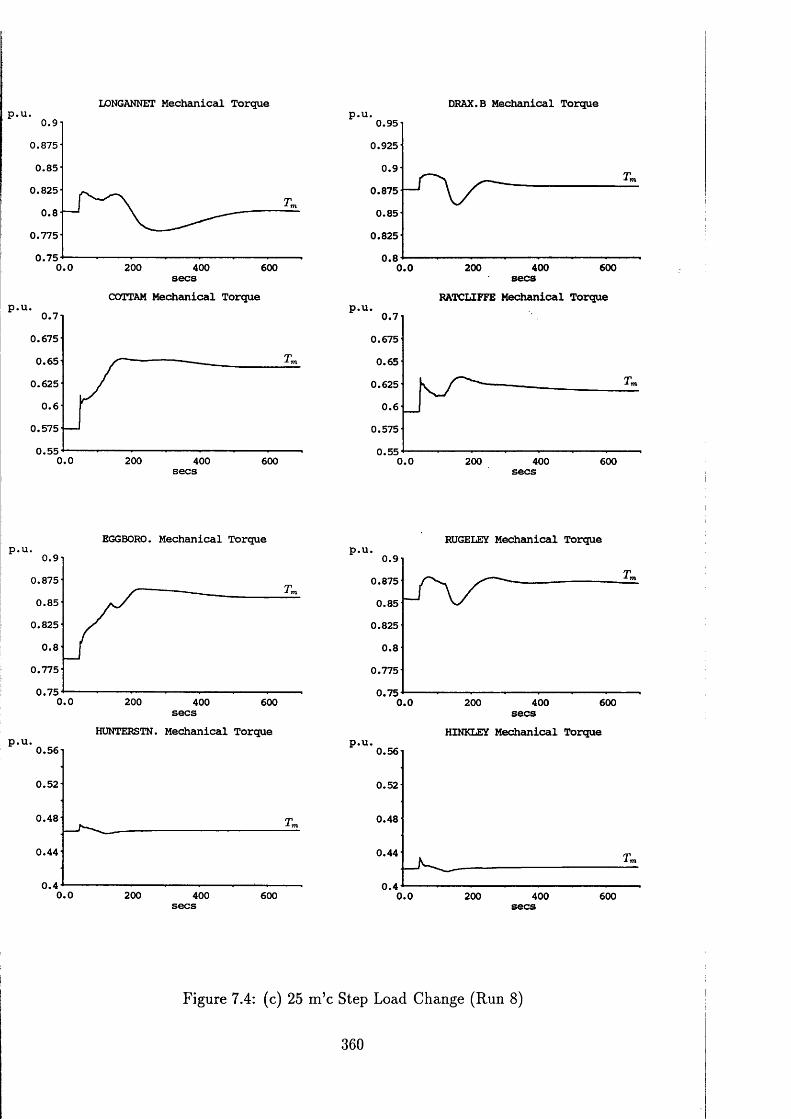
LONGANNET Mechanical Torque0.9
0 .875
0 .8 5
0 .825
0 .8
0 .775
0 .7 50.0 200 400 600secs
COTTAM Mechanical Torque0 .7
0 .675
0 .6 5
0 .625
0 . 6
0 .575
0 .5 50.0 200 400 600
DRAX.B Mechanical Torque0.95
0 .925
0 .9
0 .875
0 .85
0 .825
0.8200 400 6000.0 secs
RATCLIFFE Mechanical Torquep.u0 .7
0.675
0 .65
0.625
0 .6
0.575
0 .5 50.0 200 400 600
EGGBORO. Mechanical Torque0 .9
0.875
0 .8 5
0.825
0.80 .775
0 .7 50 .0 200 400 600secs
HUNTERSTN. Mechanical Torque0 .5 6
0 .52
0 .4 8
0 .44
0 .40.0 200 400 600
RUGELEY Mechcinical Torque0 .9
0.875
0 .85
0.825
0.8
0.775
0 .750.0 600200 400
secsHINKLEY Mechanical Torque
0 .56
0 .52
0 .48
0 .44
0 .40.0 200 400 600
Figure 7.4: (c) 25 m ’c Step Load Change (Run 8)
360

t?
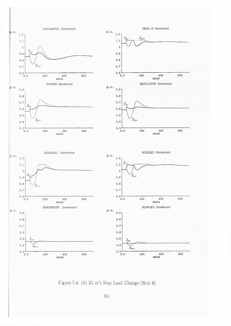
LONGANNET Governor1.21.1
igv0 .9
0.80 .7 'gvc
0.6400 6000.0 200
secsCOTTAM Governor
0 .9
0 .7
0.60 .5
'gvc0 .4
0 .30.0 200 400 600secs
EGGBORO. Governor1.2
1.1
0 .9
0.8'gvc
0 .7
0 . 6400 6000.0 200
secsHUNTERSTN. Governor
0 .9
0 .7
0 . 6
0 .5 igv0 .4 'gvc
0 .30.0 200 400 600
DRAX.B Governor1.21.1
0 .9
0.8
0 .7
0 .6400 6000 .0 200
secsRATCLIFFE Governor
0 .9
0.8
0 .7I g v
0.6
0 .5
'gvc0 .4
0 .3400 6000.0 200 secs
RUGELEY Governor1.2
igv1.1
'gvc0 .9
0.8
0 .7
0.6400 6000.0 200
secsHINKLEY Governor
0 .9
0.8
0 .7
0.60 .5
0 .4
0 .36004000 .0 200
Figure 7.4: (d) 25 m ’c Step Load Change (Run 8)
361
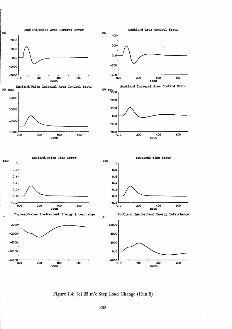
MWEngland/Wales Area Control Error Scotland Area Control Error
2000
1000
0.0
-1000
-20000.0 200 400 600
MW sec England/Wales Integral Area Control Error
50000
30000
10000
0.0 200 400 600
MW 400
200
0.0
-200
-4006004002000.0 secs
MW secScotland Integral Area Control Error
7500
5000
2500
0.0
6004000.0 200
England/Wales Time Errorsec
0.80.60 .4
0.20.0
-0.20.0 200 400 600secsEngland/Wales Inadvertent Energy InterchangeJ
2000
-6000
-10000
0.0 200 400 600
Scotland Time Errorsec
0.80.60 .4
0.20.0
-0.2 200 400 6000.0 secsScotland Inadvertent Energy Interchange
J12000
8000
4000
0.0
-40000.0 200 400 600
Figure 7.4: (e) 25 m ’c Step Load Change (Run 8)
362

6
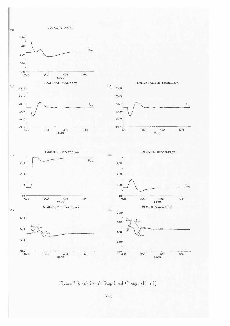
MWTie-Line Power
680
640
600
560
5200.0 200 400 600secs
Scotland FrequencyHz 50.5
50.3
50.1
49.9
49.7
49.50.0 200 400 600secs
DINORWIG1 GenerationMW
280
200
120
400.0 200 400 600secs
LONGANNET GenerationMW
660
620
580
5400.0 200 400 600
England/Wales FrequencyHz 50.5
50.3
50.1 ceg
49.9
49.7
49.5 4000.0 200 600secs
DINORWIG2 Generation
280
200
120
400.0 200 400 600secs
DRAX.B GenerationMW 700
680
660
640
6200.0 200 400 600
Figure 7.5: (a) 25 m ’c Step Load Change (Run 7)
363

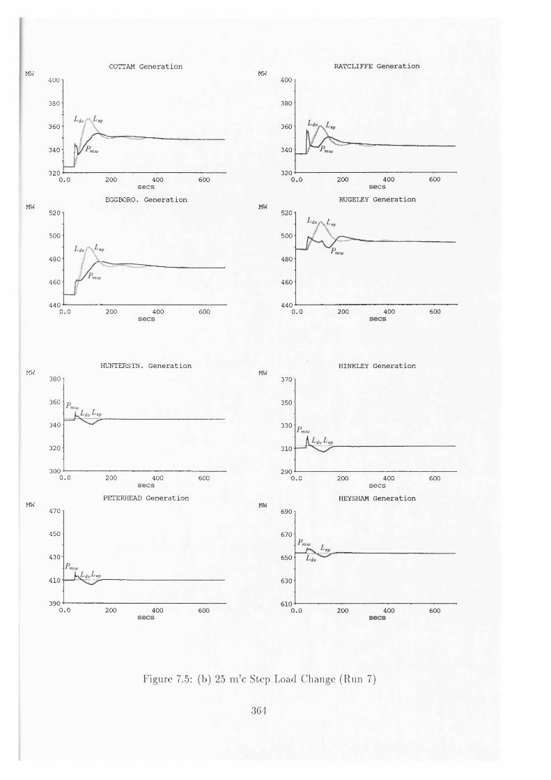
COTTAM GenerationMW
MW
400
380
360
340
3200.0 200 400 600secs
EGGBORO. Generation520
500
480
460
4400.0 200 400 600
RATCLIFFE GenerationMW
MW
400
380
360
340
320400 6000.0 200
secsRUGELEY Generation
520'sp
500
480
460
440400 6000.0 200
HUNTERSTN. GenerationMW
380
360
340
320
3000.0 200 400 600secs
PETERHEAD GenerationMW470
450
430
410
3900.0 200 400 600
HINKLEY GenerationMW
370
350
330
310
2900.0 200 400 600secs
HEYSHAM GenerationMW690
670
650
630
6100.0 200 400 600
Figure 7.5: (b) 25 m ’c Step Load Change (Run 7)
364

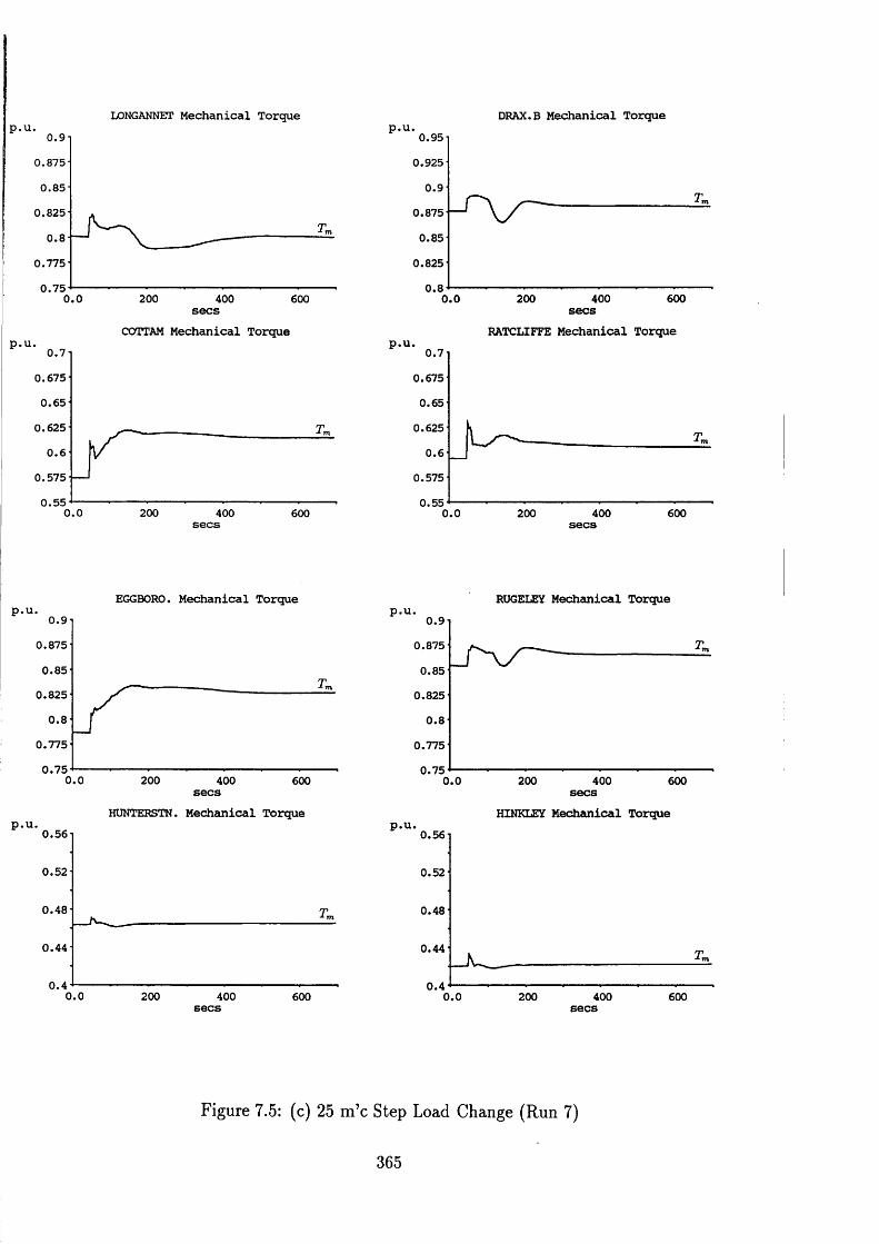
LONGANNET Mechanical Torque0.9
0.875
0 .8 5
0 .825
0.80 .775
0 .7 50.0 200 400 600secs
COTTAM Mechanical Torque0 .7
0 .675
0 .6 5
0 .625
0.60 .575
0 .5 50.0 200 400 600
DRAX.B Mechanical Torquep.u. u.yo
0.925
0 .9
0 .875
0 .85
0 .825
0.86000.0 200 400
secsRATCLIFFE Mechanical Torque
0 .7
0 .675
0 .65
0.625
0.60.575
0.556000.0 200 400
EGGBORO. Mechanical Torque0 .9
0 .875
0 .8 5
0 .825
0.80 .775
0 .7 50.0 200 400 600secs
HUNTERSTN. Mechanical Torque0 .5 6
0 .5 2
0 .4 8
0 .4 4
0 .40.0 200 400 600
RUGELEY Mechanical Torque0 .9
0.875
0 .85
0.825
0.80.775
0 .75 200 400 6000.0secs
HINKLEY Mechanical Torque0 .56
0.52
0.48
0.44
0 .40.0 200 400 600
Figure 7.5: (c) 25 m ’c Step Load Change (Run 7)
365

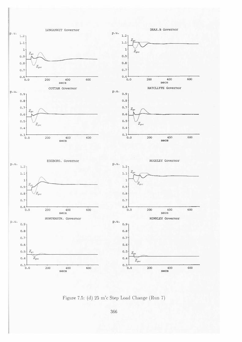
LONGANNET Governorp.u.
p.u.
1.21.1
0 .9
0.80 .7
0.6400 6000.0 200
secs COTTAM Governor
0 .9
0.80 .7
0.60 .5
'gvc0 .4
0 .3 200 400 6000.0
DRAX.B Governorp.u.
p.u.
1.21.1
0 .9
0 .7
0.6400 6002000.0 secs
RATCL1FFE Governor0 .9
0.80 .7
0.60 .5
'gvc
0 .4
0 .3400 6002000.0
EGGBORO. Governor1.21.1
i g v0 .9
0.80 .7
0.60.0 200 400 600secs
HUNTERSTN. Governorp.u.
u.y
0 .7
0.60 .5 !gv0 .4
0 .30.0 200 400 600
RUGELEY Governor1.21.1
1'gvc
0 .9
0.80 .7
0.66000.0 200 400
secsHINKLEY Governor
0 .9
0.80 .7
0.60 .5
0 .4'gvc
0 .3 200 400 6000.0
Figure 7.5: (d) 25 m ’c Step Load Change (Run 7)
366

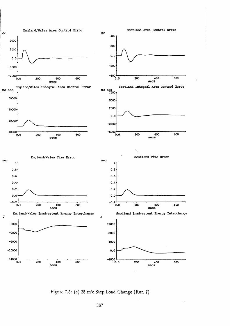
England/Wales Area Control ErrorMW
2000
1000
0.0
-1000
-20006004000 .0 200 secs
England/Wales Integral Area Control ErrorMW sec
50000
30000
10000
-100006004000 . 0 200 secs
England/Wales Time Errorsec
0 .8
0 .6
0 .4
0 .2
0 .0
- 0 . 20.0 200 400 600secs
England/Wales Inadvertent Energy InterchangeJ
2000
-2000
-6000
-10000
-140000.0 200 400 600
Scotland Area Control ErrorMW 400
200
0.0
-4006004002000.0 secs
Scotland Integral Area Control ErrorMW sec
7500
5000
2500
0.0
6004002000.0 secs
Scotland Time Errorsec
0.8
0 . 6
0 .4
0 .2
0.0- 0.2
6004002000.0 secsScotland Inadvertent Energy Interchange
J12000
8000
4000
0 .0
-40000.0 200 400 600
Figure 7.5: (e) 25 m ’c Step Load Change (Run 7)
367
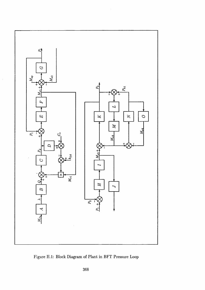
Figure H .l: Block Diagram of P lant in BFT Pressure Loop
368
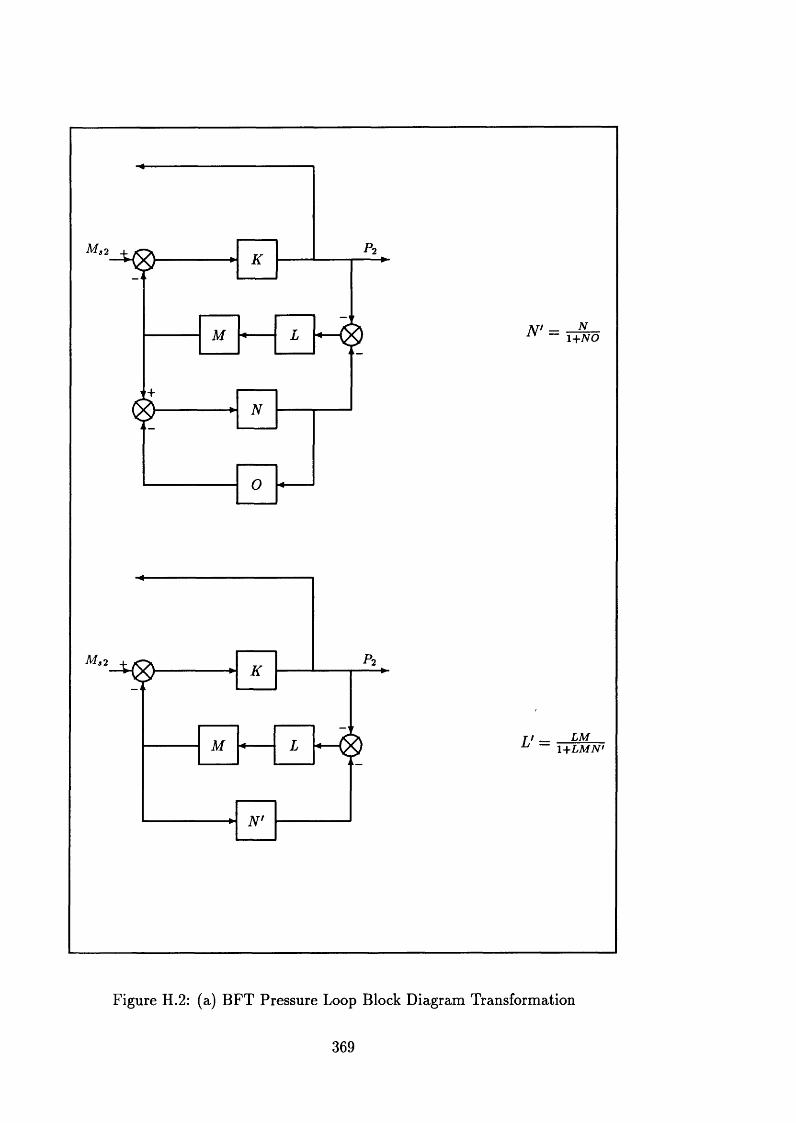
s 2
M ,3 2
v +
/ TVW' = 1+TVO
1+LMN'
Figure H.2: (a) B FT Pressure Loop Block Diagram Transformation
369
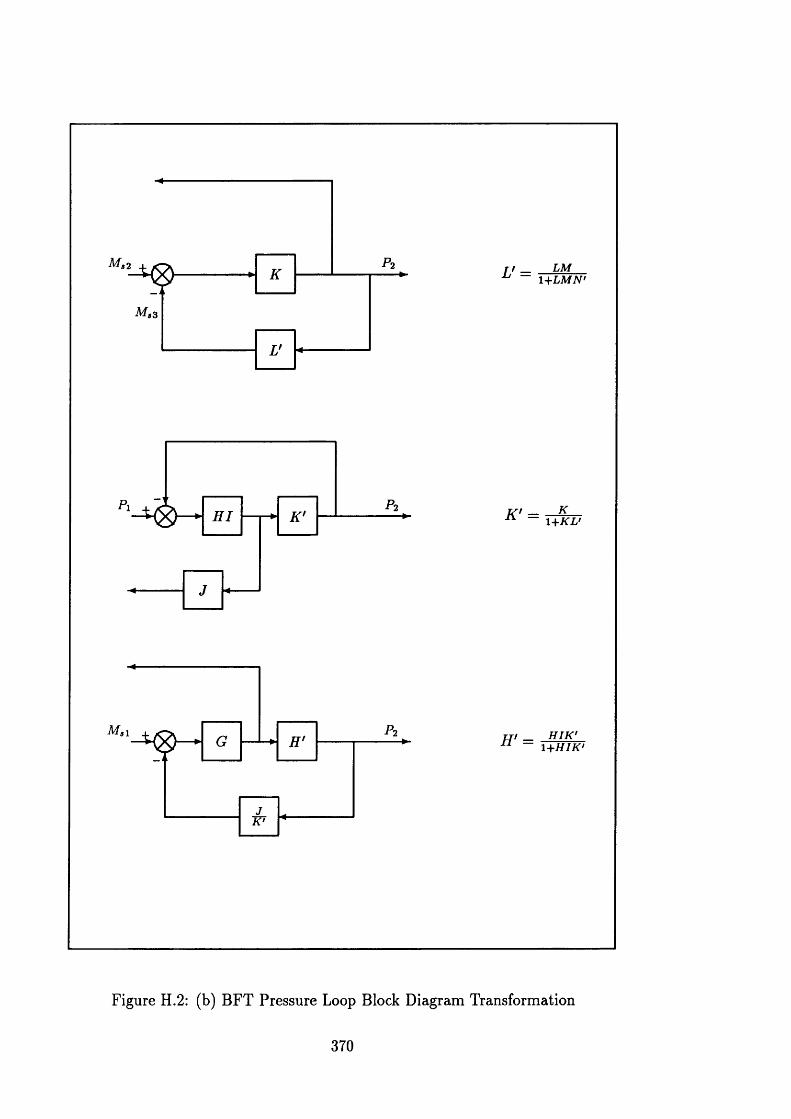
M,
_ i
M s3
K
V
P2L ' = LM
1+ L MN 1
H I K ' = 1+KL'
M ,S / _ HIK'1+ H I K 1H ' =
Figure H.2: (b) BFT Pressure Loop Block Diagram Transform ation
370
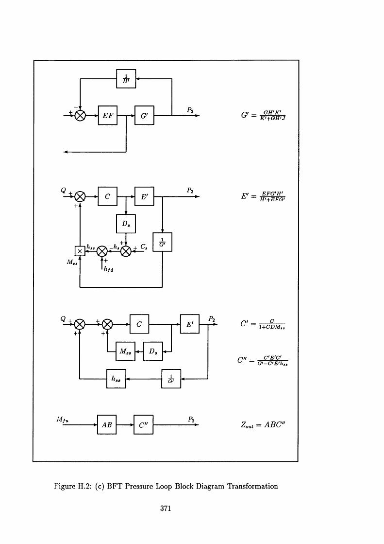
W
E F
AB
33
G ' =G H ’K '
K '+ G H 'J
/ _ E F G 'H ' H '+ E F G '
r p r £ j
E - JfT
C ' = 1+CDM ss
ft _ C 'E 'G ' G '- C 'E 'h ,C " =
Z aui = A B C "
Figure H.2: (c) BFT Pressure Loop Block Diagram Transformation
371
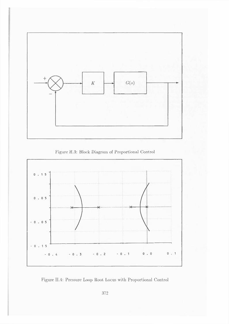
G(s)
Figure H.3: Block Diagram of Proportional Control
Figure H.4: Pressure Loop Root Locus with Proportional Control
372
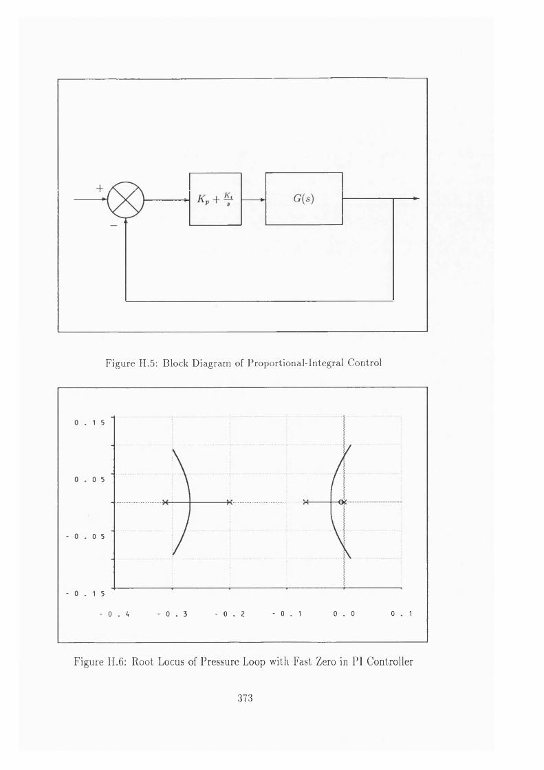
Figure H.5: Block Diagram of Proportional-Integral Control
1 5
o 5
-e<
0 5
. 1 5
- 0 . 4 - 0 . 3 - 0 . 2 - 0 . 1 0 . 0 0 . 1
Figure H.6: Root Locus of Pressure Loop with Fast Zero in PI Controller
373
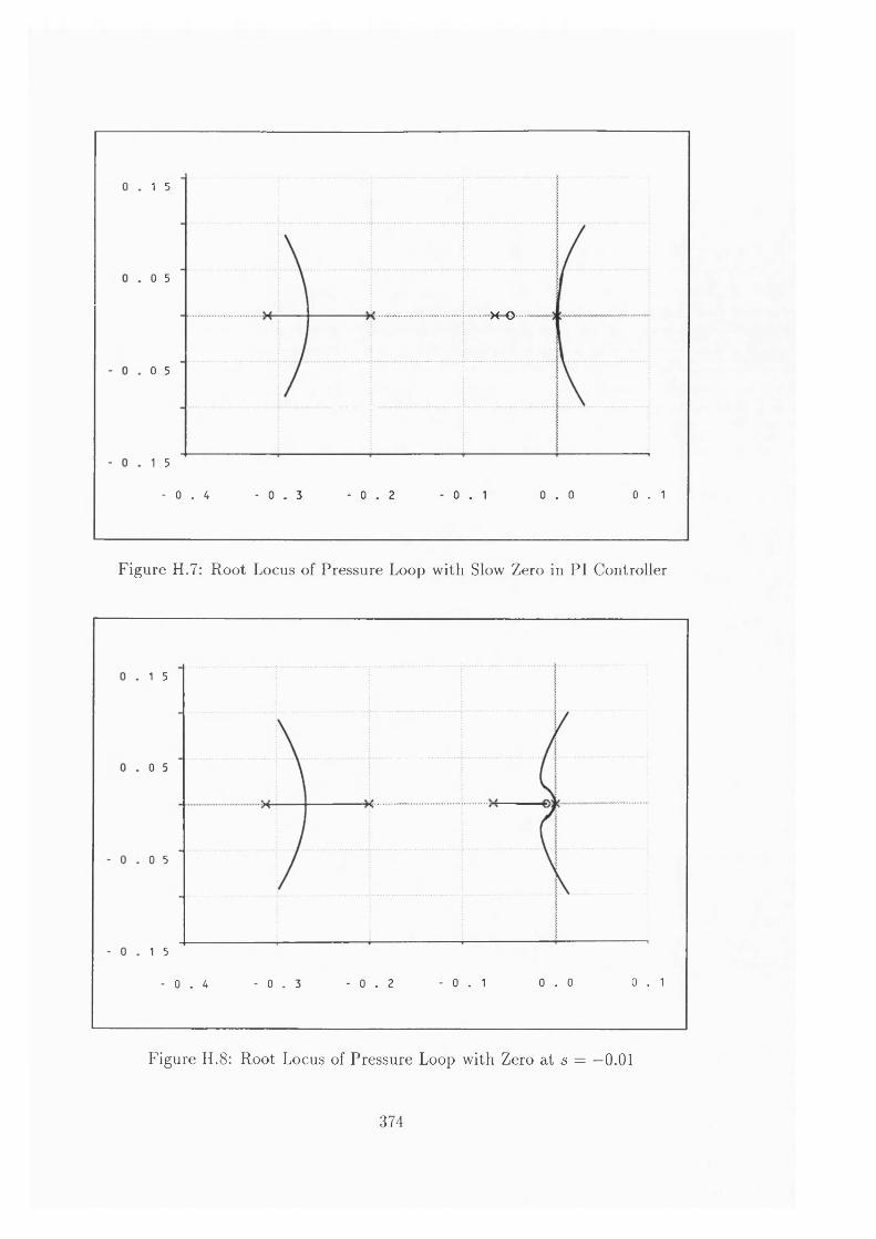
1 5
0 5
M-O
0 5
1 5
- 0 . 4 - 0 . 3 - 0 . 2 - 0 . 1 0 . 0 0 . 1
Figure H.7: Root Locus of Pressure Loop with Slow Zero in PI Controller
1 5
o 5
0 5
1 5
- 0 . 4 - 0 . 3 - 0 . 2 - 0 . 1 0 . 0 0 . 1
Figure H.8: Root Locus of Pressure Loop with Zero at s = —0.01
374
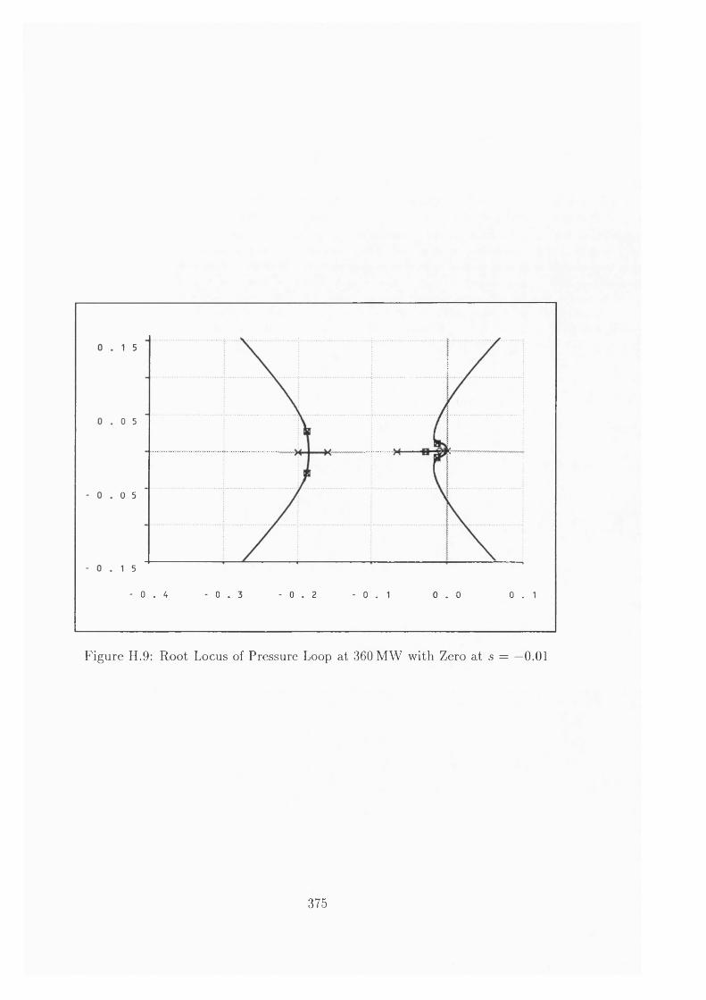
1 5
0 5
0 5
1 5
- 0 . 4 - 0 . 3 - 0 . 2 - 0 . 1 0 . 0 0 . 1
Figure H.9: Root Locus of Pressure Loop at 360 MW with Zero at s = —0.01
375
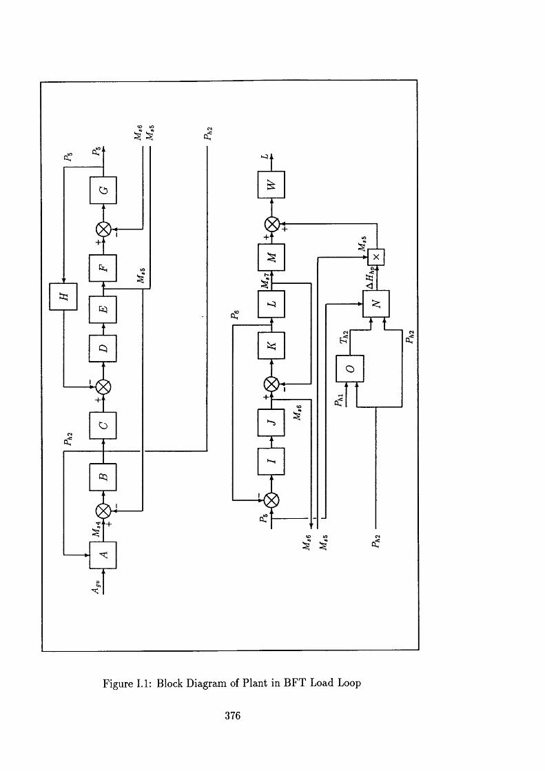
Figure 1.1: Block Diagram of Plant in B FT Load Loop
376
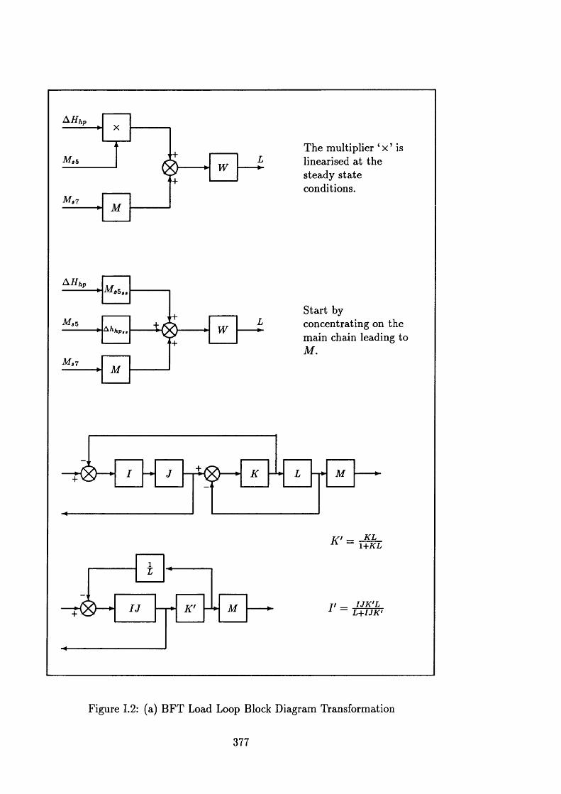
1 - +a 5
A hi
The multiplier ‘ x ’ is linearised at the steady state conditions.
Start byconcentrating on the main chain leading to M.
IJ
K' = 1+ K L
j / _ IJK'LL+IJK'
Figure 1.2: (a) B FT Load Loop Block Diagram Transformation
377
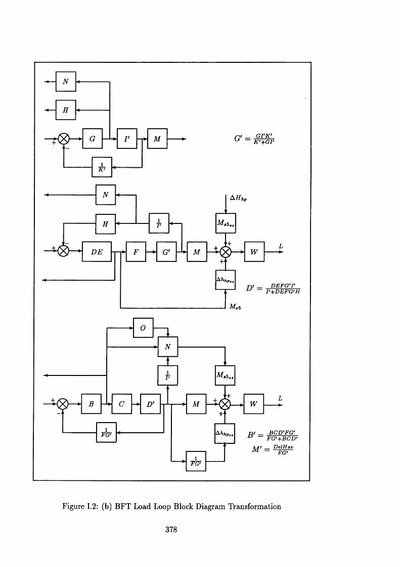
<t _ G I'K • ~ K '+G V
D E F G T~ I'+DEFG'H
K '
DE
»/ _ BCD'FG' ~ FG'+BCD
\/rt DelHssFG'
Figure 1.2: (b) B FT Load Loop Block Diagram Transformation
378
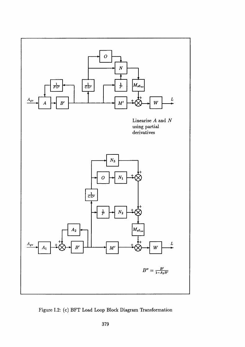
■gv
FG>
Linearise A and N using partial derivatives
CD'
O f f _ B'D ~ 1 - A 2B'
Figure 1.2: (c) BFT Load Loop Block Diagram Transformation
379
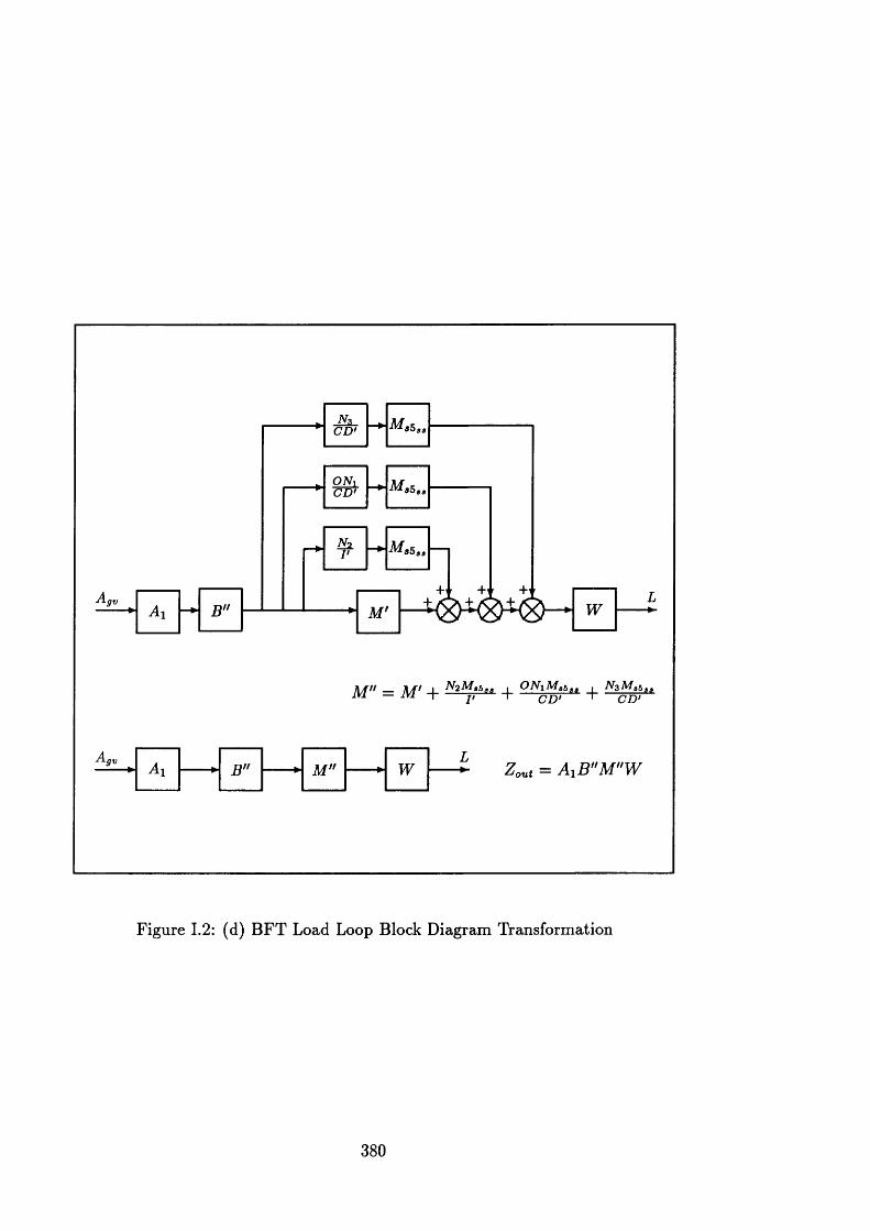
ON,C D '
M " — M ' 4- N 2 M a b °> -L O N l M **ss + N 3 M 3bsa i v i — 1V1 T T, T C D , T QD ,
Figure 1.2: (d) BFT Load Loop Block Diagram Transformation
380
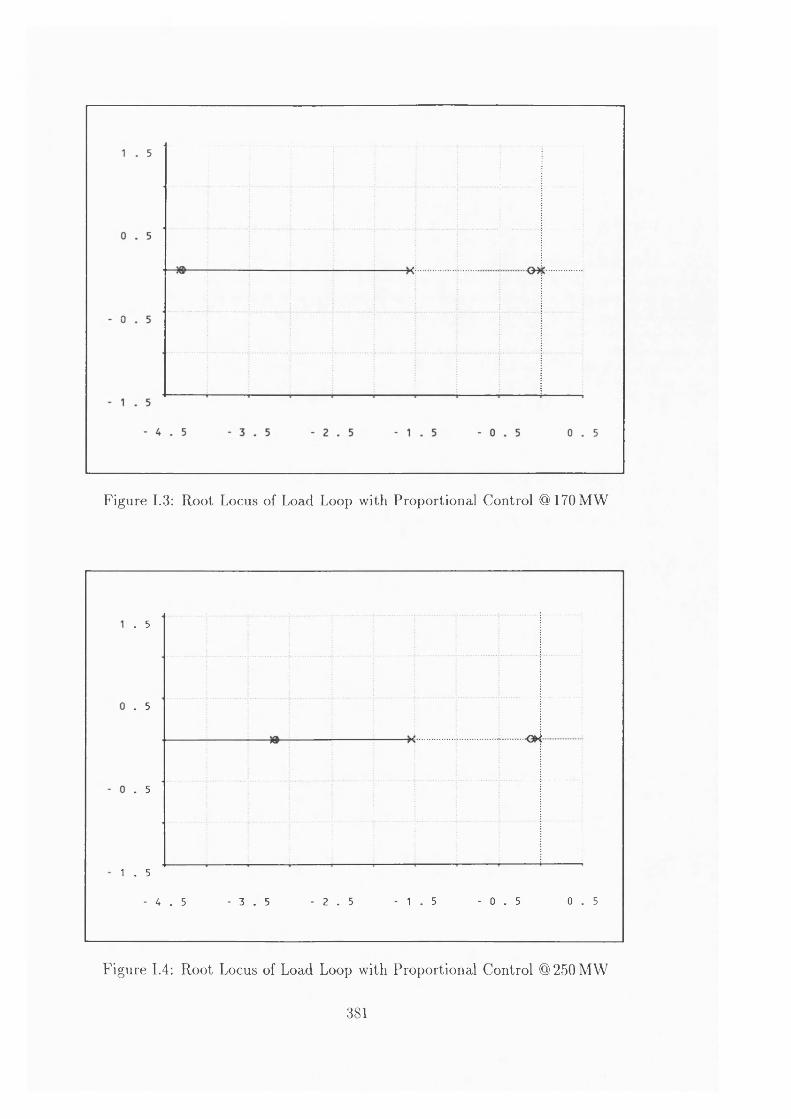
Figure 1.3: Root Locus of Load Loop with Proportional Control @170 MW
. 5
. 5
. 5
1 . 5
- 4 . 5 - 3 . 5 - 2 . 5 - 1 . 5 - 0 . 5 0 . 5
Figure 1.4: Root Locus of Load Loop with Proportional Control @ 250 MW
381
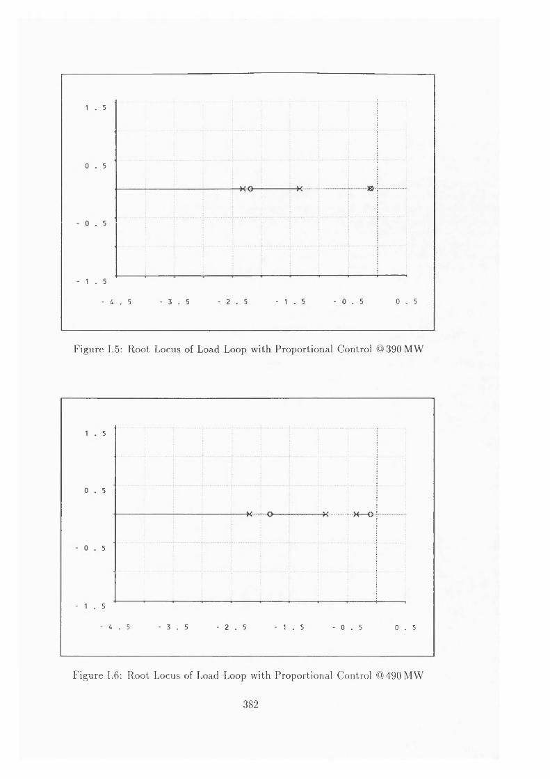
5
5
. 5
1 . 5
- 4 . 5 - 3 . 5 - 2 . 5 - 1 . 5 - 0 . 5 0 . 5
Figure 1.5: Root Locus of Load Loop with Proportional Control @390 MW
5
5
5
. 5
- 4 . 5 - 3 . 5 - 2 . 5 - 1 . 5 - 0 . 5 0 . 5
Figure 1.6: Root Locus of Load Loop with Proportional Control @ 490 MW
382
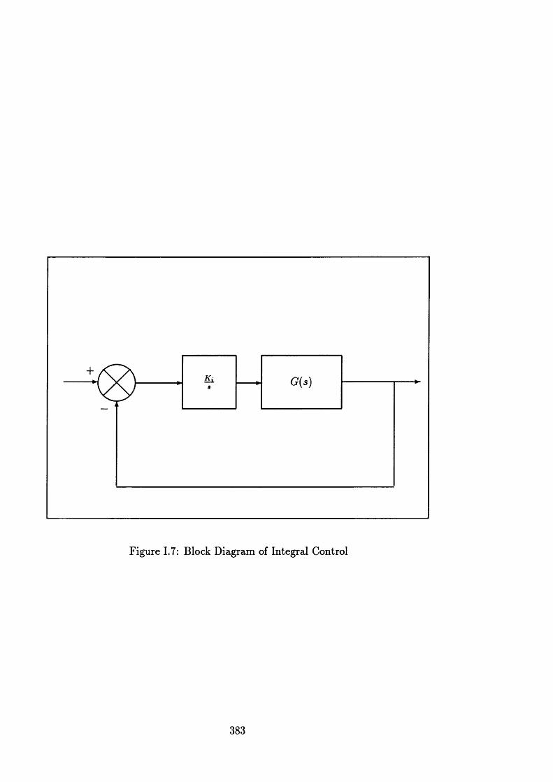
Figure 1.7: Block Diagram of Integral Control
383
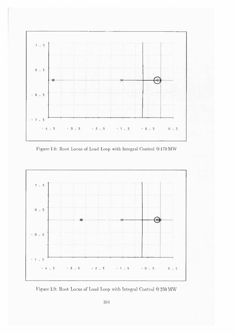
5
. 5
• • • » • • •
5
1 . 5
- 4 . 5 - 3 . 5 - 2 . 5 - 1 . 5 - 0 . 5 0 . 5
Figure 1.8: Root Locus of Load Loop with Integral Control @ 170 MW
. 5
5
5
1 . 5
- 4 . 5 - 3 . 5 - 2 . 5 - 1 . 5 - 0 . 5 0 . 5
Figure 1.9: Root Locus of Load Loop with Integral Control @250 MW
384
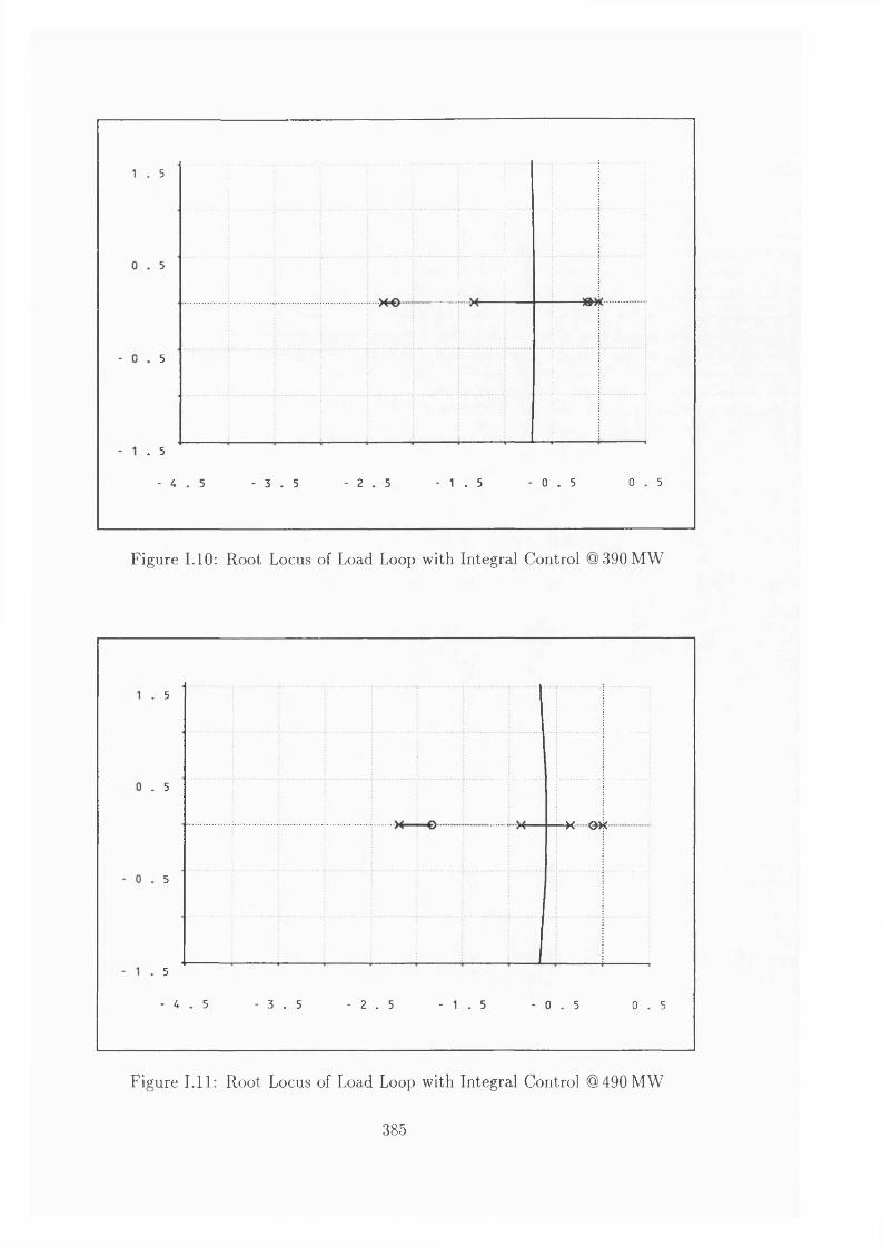
5
5
5
. 5
- 4 . 5 - 3 . 5 - 2 . 5 - 1 . 5 - 0 . 5 0 . 5
Figure 1.10: Root Locus of Load Loop with Integral Control @390 MW
. 5
. 5
—X OK
5
5
- 4 . 5 - 3 . 5 - 2 . 5 - 1 . 5 - 0 . 5 0 . 5
Figure 1.11: Root Locus of Load Loop with Integral Control @490 MW
385
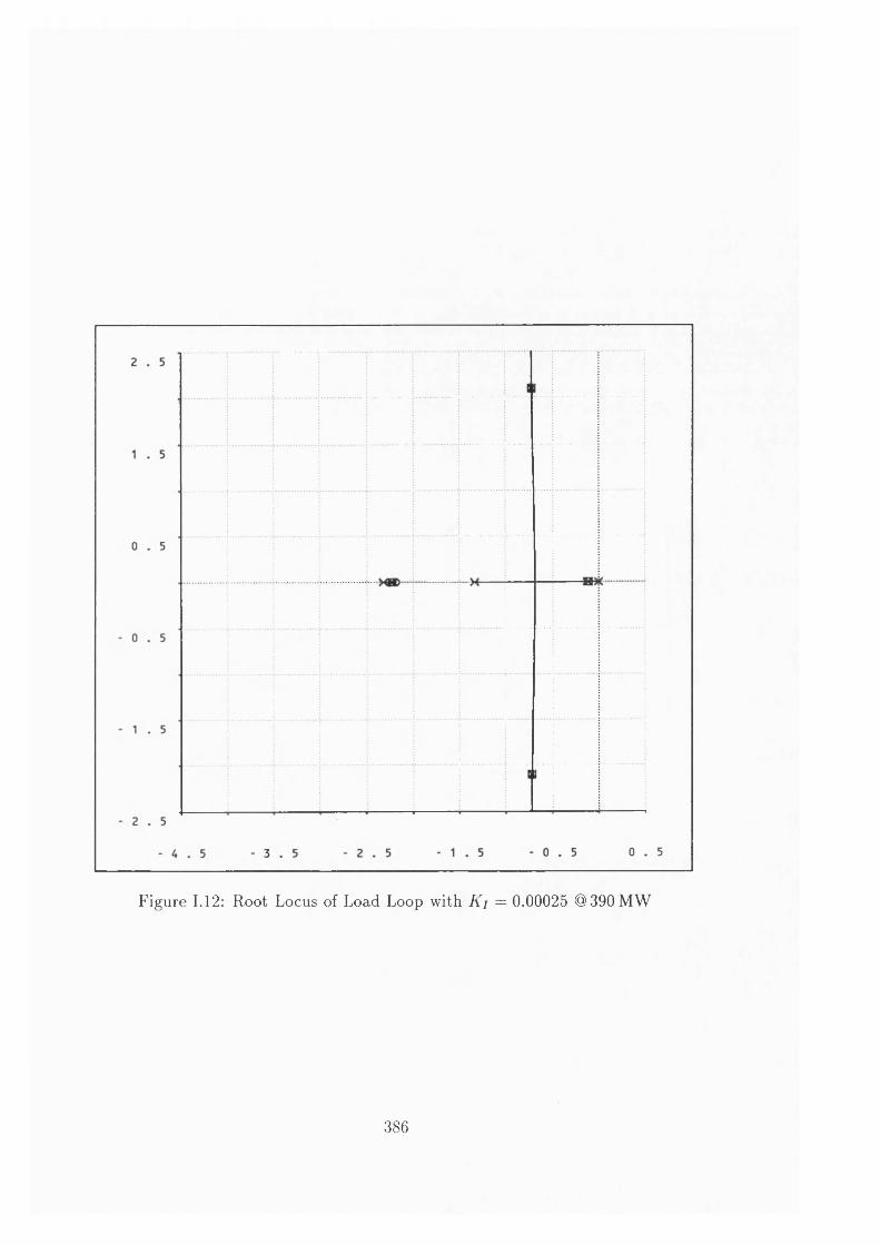
Figure 1.12: Root Locus of Load Loop with K i = 0.00025 @390 MW
386
Bibliography
[11 Electricity Council. H istory o f Electricity in Great Britain, a Chronology. Dec. 1971. Serial No. RP.3.
[2] Lord Hinton of Bankside. Heavy Current Electricity in the United Kingdom, H istory and Development. Pergamon Press, first edition, 1979. ISBN 0-08- 023246-9.
[3] F. D. Boardman. Control and operation of the UK electricity supply system: an account of its development. IEE Proceedings, 125(1 ):61—65, Jan. 1978.
[4] U. G. Knight and F. Moran. The operation and control of the CEGB power system. Trans. Inst. M C., 6(5), Oct. 1984.
[5] H. E. Pulsford. Developments in power system control. IEE Proceedings, 114(8):1139—1148, 1967.
[6] J. H. Banks, J. W. Dillow, U. G. Knight, and A. G. Oughton. Paper 2.1.6. In International Union o f Producers and D istributors of Electrical Energy D ata Processing Conference, Lisbon, June 1971.
[7] S. R. Browning, P. H. Plumptre, H. R. W. Lewis, and R. G. Lucas. Development of the generator ordering and loading program (GOAL). In UPEC-20, Huddersfield, England, 1985.
[8] P. Brown and A. G. Entwistle. Distributed computer control of a 500MW oil-fired boiler. In IEE Conf. D istributed Computer Control System s, pages 108-113, 1977.
[9] L. R. Johnstone, C. R. Marsland, and S. T. Pringle. A distributed computer control system for a 120MW boiler. In IEE Conf. D istributed Com puter Control System s, pages 114-119, 1977.
[10] M. J. Metcalfe, J. Waddington, and R. G. Wilson. Operational experience with fossil-fired generating plant under automatic load control. IEE Proceedings, 126(4), Apr. 1979.
[11] J. Waddington. Load-controller design for a regulating coal-fired unit. IEE Proceedings, 126(5), May 1979.
387
12] J. N. Wallace and R. Clarke. Load control of a 500MW oil-fired boiler- turbine. In IEE Con}. Control and its Applications, pages 250-255, 1981.
13] A. R. Fowkes, G. Wronski, and R. G. Wilson. The management of frequency response of fossil-fired power plant. In IEE 2nd Int. Conf. Power System M onitoring and Control, pages 400-405, 1986.
14] R. Clarke, J. Waddington, and J. N. Wallace. The application of Kalman filtering to the load/pressure control of coal-fired boilers. In IEE Colloq., 1988/89.
15] Central Electricity Generating Board. Annual report and accounts 1987/88, 1988.
16] R. M. Dunnett and S. Duckworth. An experimental study of centralised economic dispatch in the CEGB. In IEE 2nd Int. Conf. Power System M onitoring and Control, pages 7-12, 1986.
17] W. D. Laing and C. Brewer. The development of an on-line short-term demand prediction facility. In IEE 2nd Int. Conf. Power System Monitoring and Control, pages 1-6, 1986.
18] H. Glavitsch and J. Stoffel. Automatic generation control. International Journal o f Electrical Power and Energy System s, 2(1):21—28, Jan. 1980.
19] J. Carpentier, A. Gillon, R. Girard, Y. Jegouzo, P. Pruvot, A. Candre, F. Caraman, R. Grimonpont, F. Pellen, and P. Tournebise. Concepts, models and studies for a closed loop secure automatic generation control. In IASTED Power High Tech 89, pages 361-366, Valencia, Spain, 1989.
20] M. Davies, F. Moran, and J. I. Bird. Power/frequency characteristics of the British grid system. IEE Proceedings, 106-A: 154-162, Nov. 1958.
21] J. Osanna, H. Graner, and F. Hofmann. Frequenz- und Leistungssteuerung (Netzkennliniensteuerung) von Netzverbanden. German Patent No. 634025, Feb. 1931.
22] H. Graner. Vorschlage fur den Betrieb von Netzverbanden. Elektrotechn. Z ., 55:1069, 1934.
23] G. Darrieus. Frequenz- und Leistungsregulierung in grossen Netzverbanden. Bull, schweiz. elektrotech., 28:525, 1937.
24] A. de Quervain and W. Frey. Methods of controlling interconnected power systems. Brown Boveri Review , 44(ll):472-487, Nov. 1957.
25] G. Quazza. Noninteracting controls of interconnected electric power systems. IEEE Trans. PAS , PAS-85(7):727-741, July 1966.
26] C. W. Ross. Error adaptive control computer for interconnected power systems. IEEE Trans. PAS , PAS-85(7):742-749, July 1966.
388
[27] 0 . I. Elgerd and C. E. Fosha. Optimum megawatt-frequency control of multiarea electric energy systems. IEEE Trans. PAS , PAS-89(4):556-562, Apr. 1970.
[28] C. E. Fosha and 0 . I. Elgerd. The megawatt-frequency control problem: A new approach via optimal control theory. IEEE Trans. PAS , PAS- 89(4):563-577, Apr. 1970.
[29] H. Glavitsch and F. D. Galiana. Load-frequency control with particular emphasis on thermal power stations. In E. Handschin, editor, Real-Time Control o f Electric Power System s, pages 115-145. Elsevier, 1972.
[30] F. P. deMello, R. J. Mills, and W. F. B ’Rells. Automatic generation control, part i - process modeling. IEEE Trans. PAS , pages 710-715, Mar/Apr 1973.
[31] F. P. deMello, R. J. Mills, and W. F. B ’Rells. Automatic generation control. part ii - digital control techniques. IEEE Trans. PAS , pages 716-724, Mar/Apr 1973.
[32] A. J. Connor, F. I. Denny, J. R. Huff, T. Kennedy, C. J. Frank, and M. D. Anderson. Current operating problems associated with automatic generation control. IEEE Trans. PAS , PAS-98(l):88-96, Jan/Feb 1979. A report prepared for the System Operations Subcommittee of the Power System Engineering Committee by the Current Operational Problems Working Group (76-1).
[33] M. L. Kothari, P. S. Satsangi, and J. Nanda. Sampled-data automatic generation control of interconnected reheat thermal systems considering generation rate constraints. IEEE Trans. PAS , PAS-100(5):2334-2342, May 1981.
[34] A. Kumar and O. P. Malik. Discrete analysis of load-frequency control problem. IEE Proceedings, 113-C(4): 144-145, July 1984.
[35] S. C. Tripathy, T. S. Bhatti, C. S. Jha, O. P. Malik, and G. S. Hope. Sampled data automatic generation control analysis with reheat steam turbines and governor dead-band effects. IEEE Trans. PAS , PAS-103(5):1045-1051, May 1984.
[36] L. Basanez and J. Riera. Load frequency control behaviour with governor dead-band effects. In IEE 2nd Int. Conf. Power System M onitoring and Control, pages 23-28, 1986.
[37] E. Davison and N. Tripathi. . IEEE Trans. A C , 23:312-325, 1978.
[38] A. Kumar, O. P. Malik, and G. S. Hope. Discrete variable structure controller for load frequency control of multi-area interconnected power systems. IEE Proceedings, 134-C(2):116-122, Mar. 1987.
[39] J. Carpentier. Optimal power flows: Uses, methods and developments. In IFAC Electric Energy System s, pages 11-21, Rio de Janeiro, Brazil, 1985.
389
[40] M. L. Kothari, J. Nanda, D. P. Kothari, and D. Das. Discrete-mode automatic generation control of a two-area reheat thermal system with new area control error. IEEE Trans. P W R S , 4(2):730—738, May 1989.
[41] P. D. Henerson, H. Klaiman, J. Ginnetti, T. Snodgrass, N. Cohn, S. Bloor, and L. VansSlyck. Cost aspects of AGC, inadvertent energy and time error. IEEE Trans. P W R S , 5(1):111-118, Feb. 1990.
[42] K. Yamashita and H. Miyagi. Multivariable self-tuning regulator for load frequency control system with interaction of voltage on load demand. IEE Proceedings, 138-D(2):177-183, Mar. 1991.
[43] M. Aldeen and J. F. Marsh. Decentralised proportional-plus-integral design method for interconnected power systems. IEE Proceedings, 138-C(4):263- 274, July 1991.
[44] E. Jaggy and A. P. Longley. Implementation of an AGC-algorithm in different power systems and on different control levels. In IEE 3rd Int. Conf. Power System M onitoring and Control, pages 162-167, 1991.
[45] K. Kovacs, B. Bechtold, and K. Szendy. Adaptive automatic generation control in the Hungarian power system. In IEE Int. Conf. Power System M onitoring and Control, pages 143-148, 1980.
[46] I. Vajk, M. Vajta, L. Keviczky, R. Haber, J. Hetthessy, and K. Kovacs. Adaptive load-frequency control of the Hungarian power system. Autom ation, 21 (2):129—137, 1985.
[47] J. Auge, R. Fernandez, A. Merlin, and F. Broussolle. The new real-time computerized control system in the national control center of Electricite de France. In CIGRE Int. Conf. Large High Voltage Electric System s, 30th session , 1984. paper 39-10.
[48] J. Carpentier. The French national control center present state and developments. IEEE Trans. P W R S , PW RS-l(4):42-48, Nov. 1986.
[49] J. Carpentier, A. Candre, R. C. Girard, B. A. Heilbronn, L. P. Loevenbruck, and G. J. Nerin. Secure automatic generation control. Principle, simulation models and results. In IEE 3rd Int. Conf. Power System M onitoring and Control, pages 156-161, 1991.
[50] V. Garcia-Echave, L. Pradinas, J. M. Ferrer, F. Lasheras, and J. J. Gonzales. Regulating system for the co-ordination of the multiple AGCs of the Spanish peninsular utilities as a unique control area. Description and field experiences. In CIGRE Int. Conf. Large High Voltage Electric Systems, 30th session , 1984. Paper 39-11.
[51] J. Bistrom and K. Lindstrom. The Finnish power system control centre. IEEE Trans. P W R S , PW RS-l(4):49-55, Nov. 1986.
390
[52] P. Leman and H. Urpinen. Computer aided production planning and control in the Finnish national control centre. In IEE 2nd Int. Conf. Power System M onitoring and Control, pages 13-17, 1986.
[53] G. L. Kusic, J. A. Sutterfield, A. R. Caprez, J. L. Haneline, and B. R. Bergman. Automatic generation control for hydro systems. IEEE Trans. EC, 3(1):33—39, Mar. 1988.
[54] C. D. Vournas, E. N. Dialynas, N. Hatziargyriou, A. V. Machias, J. L. Souflis, and B. C. Papadias. A flexible AGC algorithm for the Hellenic interconnected system. IEEE Trans. PW RS, 4(l):61-68, February 1989.
[55] C. Liang. An overview of the hierarchical dispatch and control system in Taipower. IEEE Trans. PW RS, 5(4):1041-1046, Nov. 1990.
[56] K. Matsuzawa, M. Suzuki, Y. Okuhara, Y. Kishidi, Y. Kudo, and T. Ya- mashita. New energy management system for central dispatching center of Tokyo Electric Power Co., Inc. IEEE Trans. PW R S, 5(4): 1112-1117, Nov.1990.
[57] M. Power and G. Schaffer. Upgrading Ireland’s national control centre. In IEE 3rd Int. Conf. Power System M onitoring and Control, pages 198-203,1991.
[58] F. Moran. Power system automatic frequency control techniques. IEE Proceedings, 106-A:145-153, Nov. 1958.
[59] C. Brewer, G. F. Charles, C. C. M. Parish, J. N. Prewett, D. C. Salthouse, and B. J. Terry. Performance of a predictive automatic load-dispatching system. IEE Proceedings, 115(10):1577—1586, Oct. 1968.
[60] C. Brewer, J. Frost, and C. C. M. Parish. Control room in an experimental load-dispatching system for the power supply industry. IEE Proceedings, 115(2):318—324, February 1968.
[61] E. D. Farmer. Stability and noise sensitivity of a digital-analogue control system for the automatic loading of a power system. IEE Proceedings, 115(3):453—459, Mar. 1968.
[62] E. D. Farmer and M. J. Potton. Development of on-line load-prediction techniques with results from trials in the south-west region of the CEGB. IEE Proceedings, 115(10): 1549-1558, Oct. 1968.
[63] F. Moran, D. K. S. Bain, and J. S. Sohal. Development of the equipment required for the loading of turbogenerators under automatic power-system control. IEE Proceedings, 155(7):1067—1075, July 1968.
[64] F. Moran and D. R. Williams. Automatic control of power-system frequency by machine controllers. IEE Proceedings, 115(4):606-614, Apr. 1968.
391
[65] P. Pettit. Digital-computer programs for an experimental automatic load- dispatching system. IEE Proceedings, 115(4):597—605, Apr. 1968.
[66] E. D. Farmer, K. W. James, F. Moran, and P. Pettit. Development of automatic digital control of a power system from the laboratory to a field installation. IEE Proceedings, 116(3):436—444, Mar. 1969.
[67] F. Moran and J. N. Prewett. An experiment in the automatic control of power generation. Autom atica , 6:19-32, 1970.
[68] Casson, Moran, and Taylor. Development and future possibilities of automatic control on the British grid system. In Proc. 1st IFAC Congress, pages 78-85, Moscow, 1960.
[69] D. K. S. Bain. Power system model. IEE Proceedings, 114(8):1131—1138, 1967.
[70] E. D. Farmer. The economics and dynamics of system loading and regulation. In IEE Conference Publication 187, pages 125-131, 1980.
[71] M. Rafian, M. J. H. Sterling, and M. R. Irving. Real-time power system simulation. IEE Proceedings, 134-C(3):206-223, May 1987.
[72] M. Rafian, M. J. H. Sterling, and M. R. Irving. Parallel processor algorithm for power system simulation. IEE Proceedings, 135-C(4), July 1988.
[73] D. K. Whitlock. RASM05 - Revised transient stability program, version 2.0. Technical Report N S/C/P478, CEGB Computing Services Department, .
[74] L. A. Dale. Real-Tim e Modelling o f Multi-Machine Power Systems. PhD thesis, School of Electrical Engineering, University of Bath, UK, 1986.
[75] T. Berry. Real Time Simulation o f Complex Power System s using Parallel Processors. PhD thesis, School of Electrical Engineering, University of Bath, UK, 1989.
[76] K. W. Chan. A Power System Simulator to Model the Transient Mode of Operation o f the (U K) N ational Supergrid in Real-Time. PhD thesis, School of Electronic and Electrical Engineering, University of Bath, UK, 1992. To be submitted.
[77] V. Kola, A. Bose, and P. M. Anderson. Power plant models for operator training simulators. IEEE Trans. PW R S, 4(2), May 1989.
[78] B. W. Empett, R. S. Edgar, and D. R. Battlebury. SYRES01 - System response program. Technical Report M S/C/P129 STB/12/71, Central Electricity Generating Board, July 1971.
[79] P. H. Ashmole, D. R. Battlebury, and R. K. Bowdler. Power system model for large frequency disturbances. IEE Proceedings, 121 (7):601—608, July 1974.
392
[80] B. E. Murray. Model specification. Technical Report O D(S)/BEM /, CEGB Systems Operations Department, Aug. 1987. Draft.
[81] D. G. Tanner. Real Time Simulation o f Power System s. PhD thesis, School of Electrical Engineering, University of Bath, UK, 1982.
[82] S. K. Williams. Power System Optim isation and Stability Studies using Real-Time Simulation. PhD thesis, School of Electrical Engineering, University of Bath, UK, 1986.
[83] T. Berry, A. R. Daniels, R. W. Dunn, and S. Geeves. Real time power system dynamics simulation. In CIG R E Int. Conf. Large High Voltage Electric System s, pages 1-5, 1990. Paper 38-210.
[84] M. Richards and C. Whitby-Strevens. BCPL, the Language and its Compiler. Cambridge University Press, 1980. ISBN 0-521-28681-6.
[85] Motorola Inc. M C68000 16 bit Microprocessor U ser’s Manual, second edition, 1980.
[86] Motorola Inc. M C68000 16 bit Microprocessor Program m er’s Manual, 1984.
[87] T. J. King. Tripos User Guide. School of Mathematics, University of Bath, 1983.
[88] T. J. King. Tripos Programming Guide. School of Mathematics, University of Bath, 1983.
[891 T. J. King. Tripos Technical Guide. School of Mathematics, University of Bath, 1983.
[90] Motorola Inc. M C68020 32 bit Microprocessor U ser’s Manual. Prentice Hall, 1985.
[91] Motorola Inc. MC68881 32 bit Coprocessor U ser’s Manual. Prentice Hall, 1985.
[92] S. P. Harbison and G. L. Steele. C: A Reference Manual. Prentice Hall, 1987.
[93] Perihelion Software Ltd. The Helios Operating System . Prentice Hall, 1989. ISBN 0-13-386004-3.
[94] Anon. T800 transputer. Technical Report 42 1082 00, Inmos Ltd, Apr. 1987.
[95] W. M. Fu. Real time power system simulation. B.Sc. final year project report, School of Electrical Engineering, University of Bath, 1989.
[96] F. Ng. A Man Machine Interface fo r Real Time Power System Simulation. PhD thesis, School of Electronic and Electrical Engineering, University of Bath, UK, 1992. To be examined.
393
[97] Microway, Inc., Research Park, Box 79, Kingston, MA 02364, USA. N u m b e r S m a s h e r - 8 6 0 O w n e r ’s M a n u a l , 1990.
[98] D. A. Briggs. Private communication to the author. National Power Division, CEGB, 1989.
[99] D. A. Briggs. Dinorwic power station. Theoretical study of ASEA governor system dynamics. Technical Report P E D /S E S /C P K /29 , Central Electricity Generating Board, Dec. 1976.
[100] C. F. Gerald and P. 0 . Wheatley. A p p l ie d N u m e r ic a l A n a ly s i s . Addison- Wesley, 1984. ISBN 0-201-11579-4.
[101] T. Berry. Private communication to the author. School of Mechanical Engineering, University of Bath, 1991.
[102] J. M. Grzejewski. Private communication to the author. School of Electronic and Electrical Engineering, University of Bath, 1991.
[103] B. M. Weedy. E le c tr ic P o w e r S y s te m s . John Wiley & Sons Ltd., third edition, Aug. 1983. ISBN 0-471-27584-0.
[104] C. Arkell. Private communication to the author. National Grid Company,1991.
[105] R. Clarke. Private communication to the author. National Power Division, CEGB, 1989.
[106] The Rand Corporation. R E D U C E 3 M a n u a l , 1983.
[107] S. Shamail. D is t r ib u te d M e m o r y D ie s e l E n g in e S im u la t io n U sing T r a n s p u t ers. PhD thesis, School of Electrical Engineering, University of Bath, UK, 1990.
[108] R. W. Dunn, A. R. Daniels, V. G ott, and C. G. Selwyn. A new architecture of high speed performance parallel computer for use in condition monitoring of large diesel engines. In I E E In t . C on f. on S o f tw a r e E n g in e e r in g f o r R e a l
T i m e S y s t e m s , Sept. 1989.
[109] M. Hafeez. A n E x p a n d a b le I n p u t / O u t p u t a n d G r a p h ic s S y s t e m f o r D i s t r ib u te d M e m o r y P a r a l l e l C o m p u te r s . PhD thesis, School of Electrical Engineering, University of B ath, UK, 1990.
[110] Transtech. T ra n s tech T M B 0 4 U se r M a n u a l , 1989. TMB04MAN0889.
[111] Vision. B A B Y 2 8 6 M B M i n i A T - S y s t e m B o a r d R e fe r e n c e M a n u a l , 1983.
[112] The British SuperGrid System. From an original supplied by the Central Electricity Generating Board.
394


