Embed Size (px)
Citation preview
1
Test Sequen ing Algorithms with Unreliable Tests
Vijaya Raghavan
y
; Mojdeh Shakeri
y
; and Krishna Pattipati
yy
The Mathworks In .
y
24, Prime Park Way, Nati k, MA 01760
e-mail: vijay�mathworks. om
Department of Ele tri al and Systems Engineering
yy
University of Conne ti ut, Storrs, CT 06269-3157
e-mail: krishna�sol.u onn.edu
Abstra t
In this paper, we onsider imperfe t test sequen ing problems under a single fault assumption. This
is a partially observed Markov de ision problem (POMDP), a sequential multi-stage de ision problem
wherein a probability distribution failure sour e must be identi�ed using the results of imperfe t tests at
ea h stage. The optimal solution for this problem an be obtained by applying a ontinuous state Dy-
nami Programming (DP) re ursion. However, the DP re ursion is omputationally very expensive owing
to the ontinuous nature of the state ve tor omprising the probabilities of faults. In order to alleviate this
omputational explosion, we present an eÆ ient implementation of the DP re ursion. We also onsider
various problems with spe ial stru ture (parallel systems) and derive losed form solutions/index-rules
without having to resort to DP. Finally, we present various top-down graph sear h algorithms for prob-
lems with no spe ial stru ture, in luding multi-step DP, multi-step information heuristi s and ertainty
equivalen e algorithms.
1 Introdu tion
An important issue in the �eld maintenan e of systems is the imperfe t nature of tests due to improper
setup, operator error, ele tromagneti interferen e, environmental onditions, or aliasing inherent in the
signature analysis of built-in-self-tests. Typi ally, a user omplaint, whi h is a subje tive measure of system
performan e, an also be onsidered as an imperfe t test be ause it does provide some insight into the
malfun tion. Imperfe t testing introdu es an additional element of un ertainty into the diagnosti pro ess:
the pass out ome of a test does not guarantee the integrity of omponents under test (be ause the test may
have missed a fault), or a failed test out ome does not mean that one or more of the impli ated omponents
are faulty (be ause the test out ome may have been a false alarm).
The onsequen es of a test error depend on the disposition of the system after repair. If a test results in a
false alarm, a fun tioning omponent is repla ed, and a failed omponent may be left in pla e. If the system
is then returned to servi e, the system fails immediately. In the ase of missed dete tion by a test, the overall
test ould indi ate that no item has failed. In this ase, the system might be returned to servi e where it fails
immediately or it might be s rapped. Either hoi e implies a ost. Relatively little attention has been given
to imperfe t testing. Most resear h e�orts were dire ted at �nding test strategies for systems with spe ial
stru ture (parallel systems). The most omplete treatment for parallel systems with imperfe t tests is by
Firstman and Gluss [1℄ in whi h a two level testing is studied with both false alarms and missed dete tions
in tests. However, it is assumed that test errors are ultimately re overed by repeating the tests until a
proper repair is made. The test sequen e is then determined in the same manner as for perfe t testing. The
perfe t-test re he ks assure test termination with proper repair and thus fails to apture the fa t that test
errors are often unre overable. For many systems, imperfe t test results annot be re ognized either be ause
of the test design or be ause retesting is e onomi ally infeasible. In these ases, the onsequen es of test
errors o ur outside of the repair fa ility. Na hlas and Loney [2℄ presented the problem of test sequen ing
Submitted to IEEE Trans. on Systems, Man, and Cyberneti s 2
for fault diagnosis using unreliable tests for parallel systems. The obje tive of the fault diagnosis problem is
to minimize the expe ted ost required to diagnose and repair the failed omponent. They present heuristi
algorithms based on eÆ ient enumeration of permutations of test sequen es, whi h are not suitable for large
problems with arbitrary stru tures. These problems of test sequen ing with unreliable tests belong to a lass
of hypothesis testing problems with dynami information seeking. Problems in dynami sear h arise in a
wide variety of appli ations [10℄ [11℄ [12℄ [13℄ [14℄. Dynami sear h in the ontext of sequential dete tion was
extensively treated by Wald [18℄. In [15℄,[16℄,[17℄, di�erent sear h problems in the presen e of false alarms
were onsidered.
In this paper, we onsider a generalized formulation of the test sequen ing problem in the presen e of
imperfe t tests for systems of arbitrary stru ture. The test sequen ing problem in this ase is a partially
observed Markov de ision problem (POMDP) [8℄ [9℄, a sequential multi-stage de ision problem wherein a
failure sour e must be identi�ed using the results of imperfe t tests at ea h stage. The optimal solution
for this problem an be obtained by applying a ontinuous state Dynami Programming (DP) re ursion.
However, the DP re ursion is omputationally very expensive owing to the ontinuous nature of the state
ve tor omprising the probabilities of faults. In order to alleviate this omputational explosion, we present
an eÆ ient implementation of the DP re ursion. We also onsider various problems with spe ial stru ture
(parallel systems) and derive losed form solutions/index-rules without having to resort to DP. Finally,
we onsider various top-down graph sear h algorithms for problems with no spe ial stru ture, in luding
multi-step DP, multi-step information heuristi s and ertainty equivalen e algorithms. We ompare these
near-optimal algorithms with DP for small problems to gauge their e�e tiveness.
2 Optimal Test Sequen ing with Imperfe t Tests
In its simplest form, the test sequen ing problem with imperfe t tests is as follows:
1. A system with a �nite set of failure sour es S = fs
0
; s
1
; s
2
; : : : ; s
m
g is given. We make the standard
assumption that the system is servi ed frequently enough that only one or none of the faults has
o urred. The "no-fault" ondition is denoted by a dummy failure sour e s
0
;
2. The a priori probability of ea h failure sour e, p(s
i
) is known;
3. A �nite set of n available tests T = ft
1
; t
2
; : : : ; t
n
g are given, where ea h test t
j
he ks a subset of
failure sour es. The relationship between the set of failure sour es and the set of tests is represented by
a rea hability matrix R = [r
ij
℄, where r
ij
= 1 if test t
j
monitors failure sour e s
i
and r
ij
= 0 otherwise.
Sin e s
0
represents the no-fault ondition, r
0j
= 0 for all t
j
2 T ;
4. The reliability of ea h test t
j
is hara terized by the dete tion-false-alarm probability pair (P
dj
; P
fj
)
1
,
where P
dj
= Probftest t
j
fails j any of the failure sour es monitored by t
j
has failedg, and P
fj
=
Probftest t
j
fails j none of the failure sour es monitored by t
j
has failedg;
5. Ea h test t
j
(1 � j � n) osts an amount
j
measured in terms of time, or other e onomi fa tors;
6. Ea h failure sour e s
i
(1 � i � m), on e identi�ed has repair/repla ement ost
Ri
, false repair/repla ement
ost C
Fi
, and missed repair/repla ement ost C
Mi
asso iated with it.
The problem is to design a test algorithm with minimum expe ted total diagnosti ost (in ludes test-
ing and repair osts) to isolate the failure sour e, if any, with a spe i�ed level of on�den e � (typi ally,
� 2 [0:95; 0:99℄). Note that sin e the tests are imperfe t, applying the same test multiple times is useful.
Moreoever, it is assumed that the false-alarm and missed-dete tion probabilities of tests do not hange with
repeated appli ations of tests. This is in ontrast to the perfe t tests ase, where additional appli ation of
the same test does not yield any additional information. Employing the single fault assumption, the rea h-
ability matrix R, and the test reliabilities (P
dj
; P
fj
) an be ombined into a single matrix of "likelihoods",
D = [d
ij
℄, where d
ij
is given by
d
ij
= r
ij
P
dj
+ (1� r
ij
)P
fj
; (1)
where d
ij
= Probf test t
j
fails j failure sour e s
i
has o urred g.
1
Extension to the ase when (P
dj
; P
fj
) are fun tions of failure sour e s
i
is straightforward.
Submitted to IEEE Trans. on Systems, Man, and Cyberneti s 3
When tests are perfe t, that is, P
dj
= 1� P
fj
= 1 for all tests, we have d
ij
= r
ij
. This orresponds to
a perfe tly observed Markov de ision problem, and has been dis ussed extensively in [7℄. The solution to
this problem is a diagnosti de ision tree, wherein the root orresponds to the state of omplete ignoran e,
the intermediate nodes relate to states of residual ambiguity and the leaves orrespond to individual failure
sour es. The test algorithm terminates when the failed element is isolated with omplete ertainty (that is,
� = 1).
When the tests are imperfe t, the test sequen ing problem is a partially observed Markov de ision problem
(POMDP), a sequential multi-stage de ision problem wherein a failure sour e must be identi�ed using the
results of imperfe t tests at ea h stage. It an be shown [4℄ that the probabilities of failure sour es onditioned
on all the previous test results onstitute a suÆ ient statisti (i.e., ontain all the ne essary information)
for de iding the next test to be applied. Formally, let j(k) 2 f1; 2; : : : ; ng be the index of the test applied
at stage k and let O(k) 2 f0(= pass); 1(= fail)g be the out ome of test t
j(k)
. Further, let I
k�1
be the
information available to de ide on test t
j(k)
to be applied at stage k. This information in ludes all the past
tests applied and their out omes given by:
I
k�1
= f(t
j(l)
; O(l)g
k�1
l=0
: (2)
Using Bayes' rule, the onditional probabilities of hypotheses f�
i
(k) = p(s
i
jI
k
) i = 0; 1; : : : ;mg, whi h
are the information states of the de ision pro ess at ea h stage k, an be shown to evolve as
�
i
(k + 1) =
[O(k)d
ij(k)
+ (1�O(k)(1� d
ij(k)
)℄�
i
(k)
P
m
l=0
[O(k)d
lj(k)
+ (1�O(k)(1� d
lj(k)
)℄�
l
(k)
: (3)
The above re ursion is initiated with �
i
(0) = p(s
i
); i = 0; 1 : : : ;m, the a priori probability distribution of
failure sour es. The optimal test t
j(k)
is given by the dynami programming (DP) re ursion [4℄:
h
�
(f�
i
(k)g) = min
j(k)2f1;2;:::;ng
"
j(k)
+
m
X
l=0
d
lj(k)
�
l
(k)
!
h
�
��
d
ij(k)
�
i
(k)
P
m
l=0
d
lj(k)
�
l
(k)
��
+
m
X
l=0
(1� d
lj(k)
)�
l
(k)
!
h
�
��
(1� d
ij(k)
)�
i
(k)
P
m
l=0
(1� d
lj(k)
)�
l
(k)
��
#
(4)
where
j(k)
is the ost of test t
j(k)
, h
�
(f�
i
(k)g) is the optimal expe ted ost-to-go from the information state
f�
i
(k) : i = 1; 2; : : : ;mg, the terms involving h
�
inside the bra kets are the optimal osts-to-go from the
information states orresponding to the fail and pass out omes, respe tively. The terminal states of this
re ursion have known ost :
h
�
(f�
i
g) =
Ri
0
+ (1� �
i
0
)C
Fi
0
+
m
X
i=1;i 6=i
0
C
Mi
�
i
(5)
where
i
0
= argmax
i
�
i
(6)
This de�nition of terminal ost fun tion orresponds to the poli y of repairing the most likely fault. Sin e
f�
i
g are ontinuous, the above DP re ursion is ontinuous. Thus, the onsideration of imperfe t tests in
the test sequen ing problem formulation onverts a �nite (albeit large) dimensional sear h problem of the
perfe t test ase into an in�nite dimensional sto hasti ontrol problem.
3 Systems of Parallel Stru ture
Parallel systems are hara terized by a rea hability matrix R with ones on the diagonal and zeros every-
where else, for some permutation of tests. That is, every failure state is dete ted by one, and only one test.
For parallel systems, we an expli itly hara terize the optimal poli y in the perfe t test ase: at ea h state
of ambiguity, test a module with the highest ratio of probability of failure and the ost of testing the module.
For the imperfe t testing ase, su h a losed form solution annot be obtained without making additional
assumptions. However, in the following subse tions, we derive losed-form solutions for some spe ial ases.
Submitted to IEEE Trans. on Systems, Man, and Cyberneti s 4
3.1 Spe ial Case 1:
Let us spe ialize the above to a parallel system with the following assumptions:
� all test osts are equal
� exa tly one fault exists
� a test an be applied more than on e
� a fault is impli ated if its posterior probability at any stage of testing ex eeds a given threshold
(typi ally, 2 [0:95; 0:99℄)
Given this problem ontext, we onsider a greedy one-step lookahead strategy that maximizes the posterior
probability of orre t de ision assuming that a de ision would be taken at the next stage impli ating the
failure with the maximum posterior probability (MAP de ision rule).
Let � and � denote the false alarm and missed dete tion probabilities of tests (identi al for all tests).
Let �
i
(k) denote the onditional probability of failure sour e s
i
at k�th stage of testing (stage 0 is when no
tests have been applied). Let P (O
j
js
i
) denote the onditional probability of out ome O
j
2 f0; 1g of test t
j
given that s
i
is present. Given the nature of tests, we further know that,
P (O
j
js
i
) =
�
g(O
i
) = O
i
(1� �) + (1�O
i
)� for i = j
h(O
i
) = O
j
�+ (1�O
j
)(1� �) for i 6= j
(7)
Let us assume that test t
j
k
is the next test to be applied at stage k. Then, sin e the greedy approa h
orresponds to the assumption that the next test is the �nal one, the de ision rule at the next stage is to
impli ate the failure sour e s
d
su h that:
�
d
(k + 1) = max
i
�
i
(k + 1) (8)
whi h translates to,
�
d
(k)P (O(j
k
; k)js
d
) = max
i
f�
i
(k)P (O(j
k
; k)js
i
)g (9)
Let us de�ne:
P (Cjs
i
; j
k
) = Prob(Corre t De ision js
i
; j
k
) (10)
Based on (9), we an write the expression for the probability of orre t de ision as,
P (Cjs
i
; j
k
) = Pr
�
�
i
(k)g(O(j
k
; k)) � max
l6=i
f�
l
(k)h(O(j
k
; k))g
�
for j
k
= i (11)
and
P (Cjs
i
; j
k
) = Pr
�
�
i
(k)h(O(j
k
; k)) �
max
�
max
l6=i;l 6=j
k
f�
l
(k)h(O(j
k
; k))g; �
j
k
(k)g(O(j
k
; k))
��
for j
k
6= i
(12)
In order to simplify the above two equations, we de�ne:
m = argmax
i
�
i
(k) (13)
m̂ = argmax
i 6=m
�
i
(k) (14)
Let us also denote O(j
k
; k) as O
j
k
, for larity.
Then we have for i = m:
P (Cjs
m
; j
k
) = Pr(g(O
m
)�
m
(k) � h(O
m
)�
m̂
js
m
) for j
k
= m
= Pr(h(O
m̂
)�
m̂
(k) � g(O
m̂
)�
m
js
m
) for j
k
= m̂
= 0 for other values of j
k
(15)
Submitted to IEEE Trans. on Systems, Man, and Cyberneti s 5
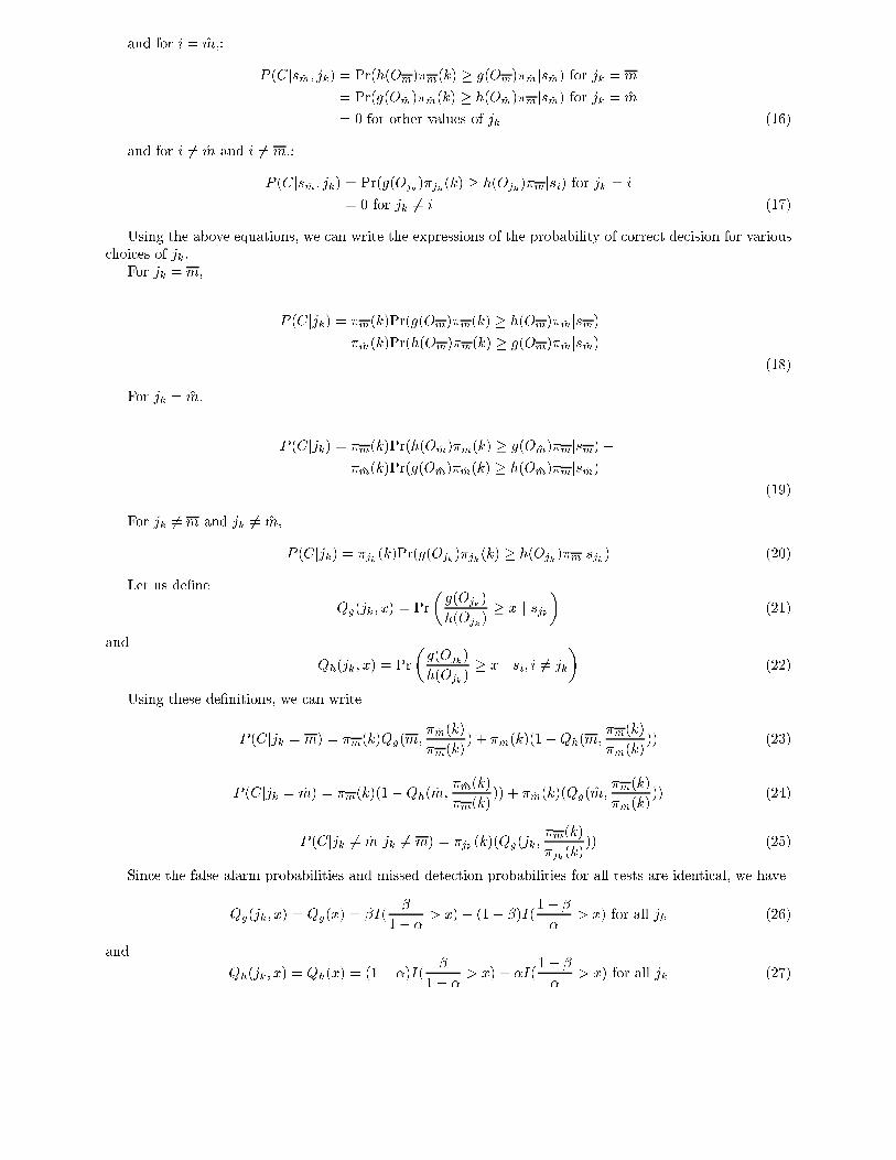
and for i = m̂,:
P (Cjs
m̂
; j
k
) = Pr(h(O
m
)�
m
(k) � g(O
m
)�
m̂
js
m̂
) for j
k
= m
= Pr(g(O
m̂
)�
m̂
(k) � h(O
m̂
)�
m
js
m̂
) for j
k
= m̂
= 0 for other values of j
k
(16)
and for i 6= m̂ and i 6= m,:
P (Cjs
m̂
; j
k
) = Pr(g(O
j
k
)�
j
k
(k) � h(O
j
k
)�
m
js
i
) for j
k
= i
= 0 for j
k
6= i (17)
Using the above equations, we an write the expressions of the probability of orre t de ision for various
hoi es of j
k
.
For j
k
= m,
P (Cjj
k
) = �
m
(k)Pr(g(O
m
)�
m
(k) � h(O
m
)�
m̂
js
m
) +
�
m̂
(k)Pr(h(O
m
)�
m
(k) � g(O
m
)�
m̂
js
m̂
)
(18)
For j
k
= m̂,
P (Cjj
k
) = �
m
(k)Pr(h(O
m̂
)�
m̂
(k) � g(O
m̂
)�
m
js
m
) +
�
m̂
(k)Pr(g(O
m̂
)�
m̂
(k) � h(O
m̂
)�
m
js
m̂
)
(19)
For j
k
6= m and j
k
6= m̂,
P (Cjj
k
) = �
j
k
(k)Pr(g(O
j
k
)�
j
k
(k) � h(O
j
k
)�
m
js
j
k
) (20)
Let us de�ne
Q
g
(j
k
; x) = Pr
�
g(O
j
k
)
h(O
j
k
)
� x j s
j
k
�
(21)
and
Q
h
(j
k
; x) = Pr
�
g(O
j
k
)
h(O
j
k
)
� x j s
i
; i 6= j
k
�
(22)
Using these de�nitions, we an write
P (Cjj
k
= m) = �
m
(k)Q
g
(m;
�
m̂
(k)
�
m
(k)
) + �
m̂
(k)(1�Q
h
(m;
�
m
(k)
�
m̂
(k)
)) (23)
P (Cjj
k
= m̂) = �
m
(k)(1�Q
h
(m̂;
�
m̂
(k)
�
m
(k)
)) + �
m̂
(k)(Q
g
(m̂;
�
m
(k)
�
m̂
(k)
)) (24)
P (Cjj
k
6= m̂ j
k
6= m) = �
j
k
(k)(Q
g
(j
k
;
�
m
(k)
�
j
k
(k)
)) (25)
Sin e the false alarm probabilities and missed dete tion probabilities for all tests are identi al, we have
Q
g
(j
k
; x) = Q
g
(x) = �I(
�
1� �
> x) + (1� �)I(
1� �
�
> x) for all j
k
(26)
and
Q
h
(j
k
; x) = Q
h
(x) = (1� �)I(
�
1� �
> x) + �I(
1� �
�
> x) for all j
k
(27)
Submitted to IEEE Trans. on Systems, Man, and Cyberneti s 6
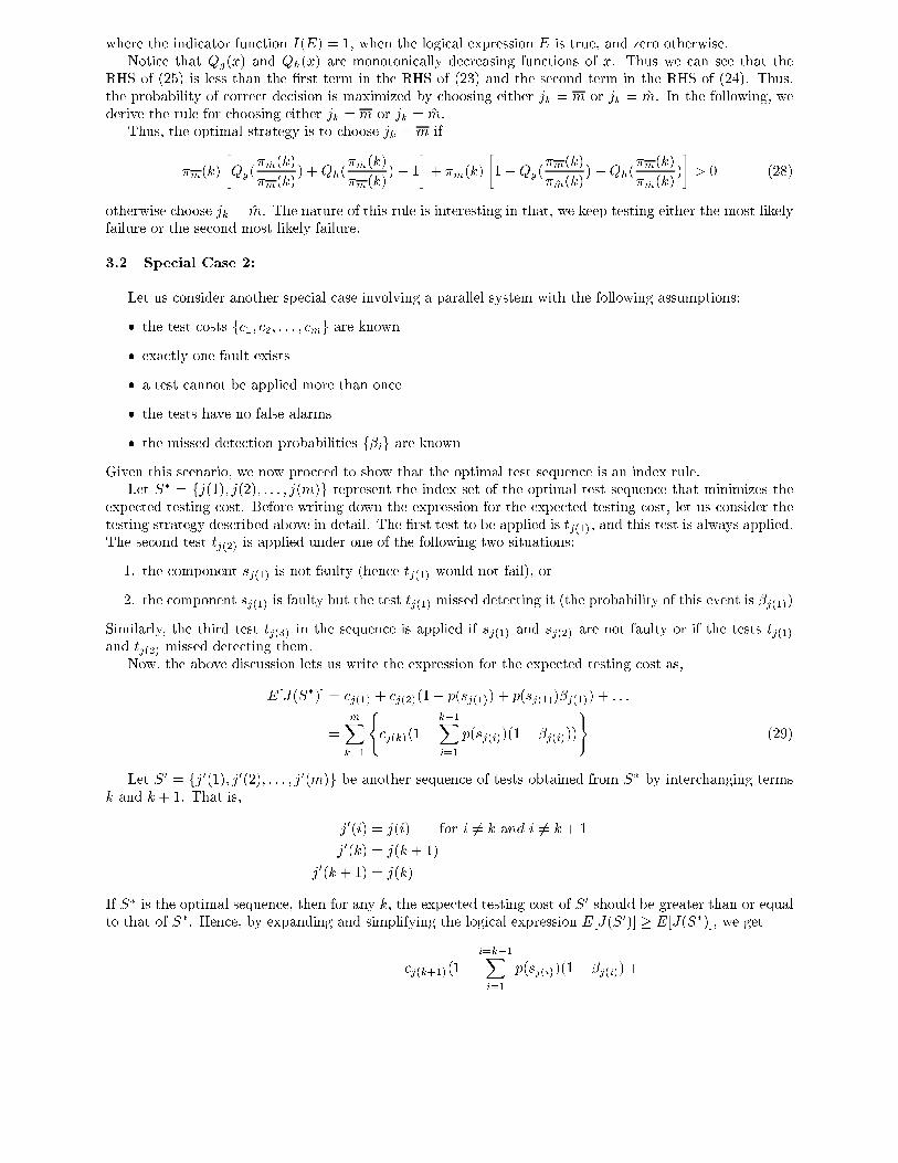
where the indi ator fun tion I(E) = 1, when the logi al expression E is true, and zero otherwise.
Noti e that Q
g
(x) and Q
h
(x) are monotoni ally de reasing fun tions of x. Thus we an see that the
RHS of (25) is less than the �rst term in the RHS of (23) and the se ond term in the RHS of (24). Thus,
the probability of orre t de ision is maximized by hoosing either j
k
= m or j
k
= m̂. In the following, we
derive the rule for hoosing either j
k
= m or j
k
= m̂.
Thus, the optimal strategy is to hoose j
k
= m if
�
m
(k)
�
Q
g
(
�
m̂
(k)
�
m
(k)
) +Q
h
(
�
m̂
(k)
�
m
(k)
)� 1
�
+ �
m̂
(k)
�
1�Q
g
(
�
m
(k)
�
m̂
(k)
)�Q
h
(
�
m
(k)
�
m̂
(k)
)
�
> 0 (28)
otherwise hoose j
k
= m̂. The nature of this rule is interesting in that, we keep testing either the most likely
failure or the se ond most likely failure.
3.2 Spe ial Case 2:
Let us onsider another spe ial ase involving a parallel system with the following assumptions:
� the test osts f
1
;
2
; : : : ;
m
g are known
� exa tly one fault exists
� a test annot be applied more than on e
� the tests have no false alarms
� the missed dete tion probabilities f�
i
g are known
Given this s enario, we now pro eed to show that the optimal test sequen e is an index rule.
Let S
�
= fj(1); j(2); : : : ; j(m)g represent the index set of the optimal test sequen e that minimizes the
expe ted testing ost. Before writing down the expression for the expe ted testing ost, let us onsider the
testing strategy des ribed above in detail. The �rst test to be applied is t
j(1)
, and this test is always applied.
The se ond test t
j(2)
is applied under one of the following two situations:
1. the omponent s
j(1)
is not faulty (hen e t
j(1)
would not fail), or
2. the omponent s
j(1)
is faulty but the test t
j(1)
missed dete ting it (the probability of this event is �
j(1)
)
Similarly, the third test t
j(3)
in the sequen e is applied if s
j(1)
and s
j(2)
are not faulty or if the tests t
j(1)
and t
j(2)
missed dete ting them.
Now, the above dis ussion lets us write the expression for the expe ted testing ost as,
E[J(S
�
)℄ =
j(1)
+
j(2)
(1� p(s
j(1)
) + p(s
j(1)
)�
j(1)
) + : : :
=
m
X
k=1
(
j(k)
(1�
k�1
X
i=1
p(s
j(i)
)(1� �
j(i)
))
)
(29)
Let S
0
= fj
0
(1); j
0
(2); : : : ; j
0
(m)g be another sequen e of tests obtained from S
�
by inter hanging terms
k and k + 1. That is,
j
0
(i) = j(i) for i 6= k and i 6= k + 1
j
0
(k) = j(k + 1)
j
0
(k + 1) = j(k)
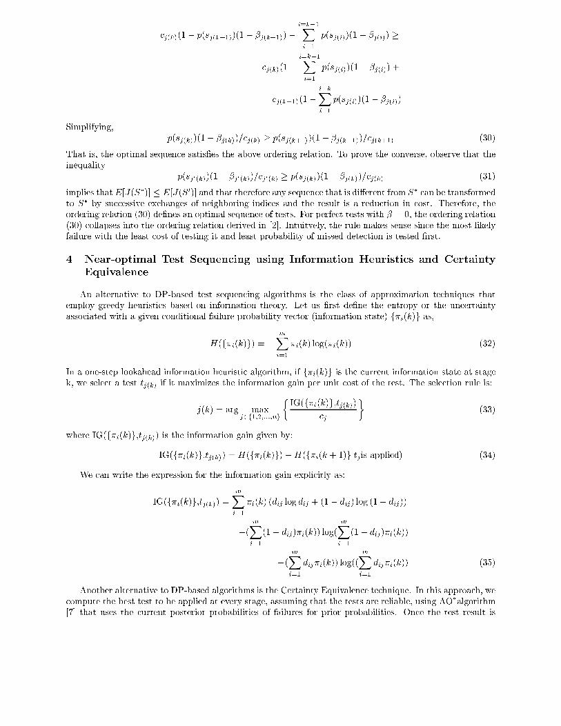
If S
�
is the optimal sequen e, then for any k, the expe ted testing ost of S
0
should be greater than or equal
to that of S
�
. Hen e, by expanding and simplifying the logi al expression E[J(S
0
)℄ � E[J(S
�
)℄, we get
j(k+1)
(1�
i=k�1
X
i=1
p(s
j(i)
)(1� �
j(i)
) +
Submitted to IEEE Trans. on Systems, Man, and Cyberneti s 7
j(k)
(1� p(s
j(k+1)
)(1� �
j(k+1)
)�
i=k�1
X
i=1
p(s
j(i)
)(1� �
j(i)
) �
j(k)
(1�
i=k�1
X
i=1
p(s
j(i)
)(1� �
j(i)
) +
j(k+1)
(1�
i=k
X
i=1
p(s
j(i)
)(1� �
j(i)
)
Simplifying,
p(s
j(k)
)(1� �
j(k)
)=
j(k)
� p(s
j(k+1)
)(1� �
j(k+1)
)=
j(k+1)
(30)
That is, the optimal sequen e satis�es the above ordering relation. To prove the onverse, observe that the
inequality
p(s
j
0
(k)
)(1� �
j
0
(k)
)=
j
0
(k)
� p(s
j(k)
)(1� �
j(k)
)=
j(k)
(31)
implies that E[J(S
�
)℄ � E[J(S
0
)℄ and that therefore any sequen e that is di�erent from S
�
an be transformed
to S
�
by su essive ex hanges of neighboring indi es and the result is a redu tion in ost. Therefore, the
ordering relation (30) de�nes an optimal sequen e of tests. For perfe t tests with � = 0, the ordering relation
(30) ollapses into the ordering relation derived in [2℄. Intuitvely, the rule makes sense sin e the most likely
failure with the least ost of testing it and least probability of missed dete tion is tested �rst.
4 Near-optimal Test Sequen ing using Information Heuristi s and Certainty
Equivalen e
An alternative to DP-based test sequen ing algorithms is the lass of approximation te hniques that
employ greedy heuristi s based on information theory. Let us �rst de�ne the entropy or the un ertainty
asso iated with a given onditional failure probability ve tor (information state) f�
i
(k)g as,
H(f�
i
(k)g) = �
m
X
i=1
�
i
(k) log(�
i
(k)) (32)
In a one-step lookahead information heuristi algorithm, if f�
i
(k)g is the urrent information state at stage
k, we sele t a test t
j(k)
if it maximizes the information gain per unit ost of the test. The sele tion rule is:
j(k) = arg max
j2f1;2;:::;ng
�
IG(f�
i
(k)g,t
j(k)
)
j
�
(33)
where IG(f�
i
(k)g,t
j(k)
) is the information gain given by:
IG(f�
i
(k)g,t
j(k)
) = H(f�
i
(k)g)�H(f�
i
(k + 1)gjt
j
is applied) (34)
We an write the expression for the information gain expli itly as:
IG(f�
i
(k)g,t
j(k)
) =
m
X
i=1
�
i
(k) (d
ij
log d
ij
+ (1� d
ij
) log (1� d
ij
))
�(
m
X
i=1
(1� d
ij
)�
i
(k)) log(
m
X
i=1
(1� d
ij
)�
i
(k))
�(
m
X
i=1
d
ij
�
i
(k)) log((
m
X
i=1
d
ij
�
i
(k)) (35)
Another alternative to DP-based algorithms is the Certainty Equivalen e te hnique. In this approa h, we
ompute the best test to be applied at every stage, assuming that the tests are reliable, using AO
�
algorithm
[7℄ that uses the urrent posterior probabilities of failures for prior probabilities. On e the test result is
Submitted to IEEE Trans. on Systems, Man, and Cyberneti s 8
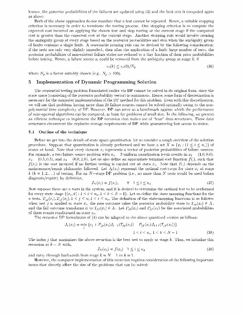
known, the posterior probabilities of the failures are updated using (3) and the best test is omputed again
as above.
Both of the above approa hes do not mandate that a test annot be repeated. Hen e, a suitable stopping
riterion is ne essary in order to terminate the testing pro ess. One stopping riterion is to ompute the
expe ted ost in urred on applying the hosen test and stop testing at the urrent stage if the omputed
ost is greater than the expe ted ost at the urrent stage. Another stopping rule would involve pruning
the ambiguity group at every stage based on the posterior probabilities and stop when the ambiguity group
of faults ontains a single fault. A reasonable pruning rule an be devised by the following onsideration:
if the tests are only very slightly imperfe t, then after the appli ation of a fairly large number of tests, the
posterior probabilities of non-existent failure states are redu ed to a tiny fra tion of their prior probabilities
before testing. Hen e, a failure sour e s
i
ould be removed from the ambiguity group at stage k, if
�
i
(k) � �
i
(0)=N
p
(36)
where N
p
is a fa tor suitably hosen (e.g., N
p
> 100).
5 Implementation of Dynami Programming Solution
The sequential testing problem formulated earlier via DP annot be solved in its original form, sin e the
state spa e ( onsisting of the posterior probability ve tor) is ontinuous. Hen e, some form of dis retization is
ne essary for the omputer implementation of the DP method for this problem. Even with this dis retization,
we will see that problems having more than 20 failure sour es annot be solved optimally owing to the non-
polynomial time omplexity of DP. However, DP an serve as a ben hmark against whi h the performan e
of near-optimal algorithms an be ompared, at least for problems of small size. In the following, we present
an eÆ ient te hnique to implement the DP re ursion that makes use of \lean" data stru tures. These data
stru tures ir umvent the explosive storage requirements of DP, while guaranteeing fast a ess to states.
5.1 Outline of the te hnique
Before we get into the details of state spa e quantization, let us onsider a rough overview of the solution
pro edure. Suppose that quantization is already performed and we have a set X = fx
i
: (1 � i � n
s
)g of
states at hand. Note that every element x
i
represents a ve tor of posterior probabilities of failure sour es.
For example, a two failure sour e problem with n
s
= 3 uniform quantization levels results in x
1
= (1:0; 0:0),
x
2
= (0:5; 0:5), and x
3
= (0:0; 1:0). Let us also de�ne an appropriate terminal ost fun tion f(:), su h that
f(x
i
) is the ost in urred if no further testing is arried out at state x
i
. Note that f(:) depends on the
maintenan e/repair philosophy followed. Let J
k
(x
i
) represent the optimal ost-to-go for state x
i
at stage
k (k = 1; 2; : : :) of testing. For an N�stage DP problem (i.e., no more than N tests would be used before
diagnosis/repair), by de�nition,
J
N
(x
i
) = f(x
i
); 8 1 � i � n
s
(37)
Now suppose there are n tests in the system, and it is desired to determine the optimal test to be performed
for every state-stage f(x
i
; k) : 1 � i � n
s
; 1 � k � N � 1g. Let us de�ne the state-mapping fun tions for the
n tests, T
jp
(x
i
); T
jf
(x
i
); 1 � j � n; 1 � i � n
s
, The de�nition of the state-mapping fun tions is as follows:
when test j is applied at state x
i
, the pass out ome takes the posterior probability state to T
jp
(x
i
) 2 X ,
and the fail out ome transforms it to T
jf
(x
i
) 2 X . Let P
jp
(x
i
) and P
jf
(x
i
) be the asso iated probabilities
of these events onditioned on state x
i
.
The re ursive DP formulation of (4) an be adapted to the above quantized version as follows:
J
k
(x
i
) = min
j
f
j
+ P
jp
(x
i
)J
k+1
(T
jp
(x
i
)) + P
jf
(x
i
)J
k+1
(T
jf
(x
i
))g
1 � i � n
s
; 1 � k � N � 1 (38)
The index j that maximizes the above re ursion is the best test to apply at stage k. Thus, we initialize this
re ursion at k = N with,
J
N
(x
i
) = f(x
i
) 1 � i � n
s
(39)
and arry through ba kwards from stage k = N � 1 to k = 1.
However, the omputer implementation of this re ursion requires onsideration of the following important
issues that dire tly a�e t the size of the problems that an be solved:
Submitted to IEEE Trans. on Systems, Man, and Cyberneti s 9
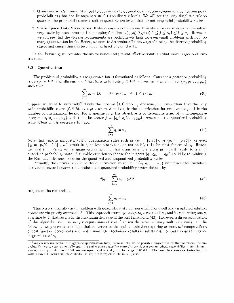
1. Quantization S heme: We need to determine the optimal quantization s heme to map oating point
probabilities (that an lie anywhere in [0,1℄) to dis rete levels. We will see that any simplisti rule to
quantize the probabilities may result in quantization levels that do not map valid probability states.
2. State Spa e Data Stru tures: If the storage is not an issue, then the above re ursions an be solved
very easily by pre omputing the mapping fun tions T
jp
(x
i
); T
jf
(x
i
); 1 � j � n; 1 � i � n
s
. However,
we will see that the storage requirements are prohibitively high for even small problems with not too
many quantization levels. Hen e, we need to determine eÆ ient ways of storing the dis rete probability
states and omputing the test-mapping fun tions on the y.
In the following, we onsider the above issues and present e�e tive solutions that make larger problems
tra table.
5.2 Quantization
The problem of probability state quantization is formulated as follows. Consider a posterior probability
state spa e P
m
of m dimensions. That is, a valid state p 2 P
m
is a ve tor of m elements fp
1
; p
2
; : : : ; p
m
g
su h that,
m
X
i=1
p
i
= 1:0 0 � p
i
� 1 8 1 � i � m (40)
Suppose we want to uniformly
2
divide the interval [0; 1℄ into n
q
divisions, i.e., we ordain that the only
valid probabilities are f0; Æ; 2Æ; : : : ; n
q
Æg, where Æ = 1=n
q
is the quantization interval, and n
q
+ 1 is the
number of quantization levels. For a spe i�ed n
q
, the obje tive is to determine a set of m non-negative
integers fq
1
; q
2
; : : : ; q
m
g su h that the ve tor p̂ = fq
1
Æ; q
2
Æ; : : : ; q
m
Æg represents the quantized probability
state. Clearly, it is ne essary to have,
m
X
i=1
q
i
= n
q
(41)
Note that various simplisti s alar quantization rules su h as fq
i
= dp
i
=Æeg, or fq
i
= bp
i
=Æ g, or even
fq
i
= bp
i
=Æ + 0:5 g, will result in quantized states that do not satisfy (41) for most hoi es of n
q
. Hen e,
we need to devise a ve tor quantization s heme, that transforms any given probability state to a valid
quantized probability state. A suitable riterion to hoose the integers fq
1
; q
2
; : : : ; q
m
g ould be to minimize
the Eu lidean distan e between the quantized and unquantized probability states.
Formally, the optimal hoi e of the quantization ve tor q = fq
1
; q
2
; : : : ; q
m
g minimizes the Eu lidean
distan e measure between the absolute and quantized probability states de�ned by,
d(q) =
m
X
i=1
(p
i
� q
i
Æ)
2
(42)
subje t to the onstraint,
m
X
i=1
q
i
= n
q
(43)
This is a resour e allo ation problem with quadrati ost fun tion whi h has a well-known optimal solution
pro edure via greedy approa h [5℄. This approa h starts by assigning zeros to all q
i
, and in rementing one q
i
at a time by 1, that results in the maximum de rease of the ost fun tion in (42). However, a dire t appli ation
of this algorithm requires mn
q
omputations of ost fun tion de rements (mn
q
multipli ations). In the
following, we present a te hnique that onverges to the optimal solution requiring at most m
2
omputations
of ost fun tion de rements and m divisions. Our te hnique results in substantial omputational savings for
large values of n
q
.
2
We do not use order of magnitude quantization here, be ause, the set of possible traje tories of the onditional failure
probability ve tor an potentially span the entire state-spa e.For example, onsider a system whose rea hability matrix is non-
sparse, prior probabilities of failures are equal, and � and � in the range [0.05,0.1℄. The possible state-traje tories for this
system are not ne essarily on entrated in any given region in the state-spa e.
Submitted to IEEE Trans. on Systems, Man, and Cyberneti s 10
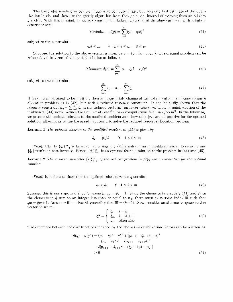
The basi idea involved in our te hnique is to ompute a fast, but a urate �rst estimate of the quan-
tization levels, and then use the greedy algorithm from that point on, instead of starting from an all-zero
q ve tor. With this in mind, let us now onsider the following version of the above problem with a tighter
onstraint set:
Minimize d(q) =
m
X
i=1
(p
i
� q
i
Æ)
2
(44)
subje t to the onstraint,
q
i
Æ � p
i
8 1 � i � m; 0 � q
i
(45)
Suppose, the solution to the above version is given by q̂ = fq̂
1
; q̂
2
; : : : ; q̂
m
g. The original problem an be
reformulated in terms of this partial solution as follows:
Minimize d(r) =
m
X
i=1
(p
i
� q̂
i
Æ � r
i
Æ)
2
(46)
subje t to the onstraint,
m
X
i=1
r
i
= n
q
�
m
X
i=1
q̂
i
(47)
If fr
i
g are onstrained to be positive, then an appropriate hange of variables results in the same resour e
allo ation problem as in (42), but with a redu ed resour e onstraint. It an be easily shown that the
resour e onstraint n
q
�
P
m
i=1
q̂
i
in the redu ed problem an never ex eed m. Then, a qui k solution of the
problem in (44) would redu e the number of ost fun tion omputations from mn
q
to m
2
. In the following,
we present the optimal solution to the modi�ed problem and show that fr
i
g are all positive for the optimal
solution, allowing us to use the greedy approa h to solve the redu ed resour e allo ation problem.
Lemma 1 The optimal solution to the modi�ed problem in (44) is given by,
q̂
i
= bp
i
=Æ 8 1 � i � m (48)
Proof: Clearly fq̂
i
g
m
i=1
is feasible. In reasing any fq̂
i
g results in an infeasible solution. De reasing any
fq̂
i
g results in ost in rease. Hen e, fq̂
i
g
m
i=1
is an optimal feasible solution to the problem in (44) and (45).
Lemma 2 The resour e variables fr
i
g
m
i=1
of the redu ed problem in (46) are non-negative for the optimal
solution.
Proof: It suÆ es to show that the optimal solution ve tor q satis�es
q
i
� q̂
i
8 1 � i � m (49)
Suppose this is not true, and that for some k, q
k
= q̂
k
� 1. Sin e the elements in q satisfy (41) and sin e
the elements in q̂ sum to an integer less than or equal to n
q
, there must exist some index m su h that
q
m
= q̂
m
+1. Assume without loss of generality that m = (k+1). Now, onsider an alternative quantization
ve tor q
a
where,
q
a
i
=
8
<
:
q̂
k
i = k
q̂
m
i = k + 1
q
i
otherwise
(50)
The di�eren e between the ost fun tions indu ed by the above two quantization ve tors an be written as,
d(q)� d(q
a
) = (p
k
� q̂
k
Æ � Æ)
2
+ (p
k+1
� q̂
k+1
Æ + Æ)
2
�(p
k
� q̂
k
Æ)
2
� (p
k+1
� q̂
k+1
Æ)
2
= Æ[p
k+1
� q̂
k+1
Æ + (q̂
k
+ 1)Æ � p
k
)℄
� 0 (51)
Submitted to IEEE Trans. on Systems, Man, and Cyberneti s 11
The �nal inequality in the above equation follows dire tly from the de�nition of q̂
i
= bp
i
=Æ , implying p
i
� q̂
i
and (q̂
i
+ 1)Æ � p
i
. Thus we see that a solution q violating the statement of the lemma annot be optimal.
Hen e, it follows that the optimal solution always ontains q̂ thereby for ing the variables r
i
in (46) to be
non-negative.
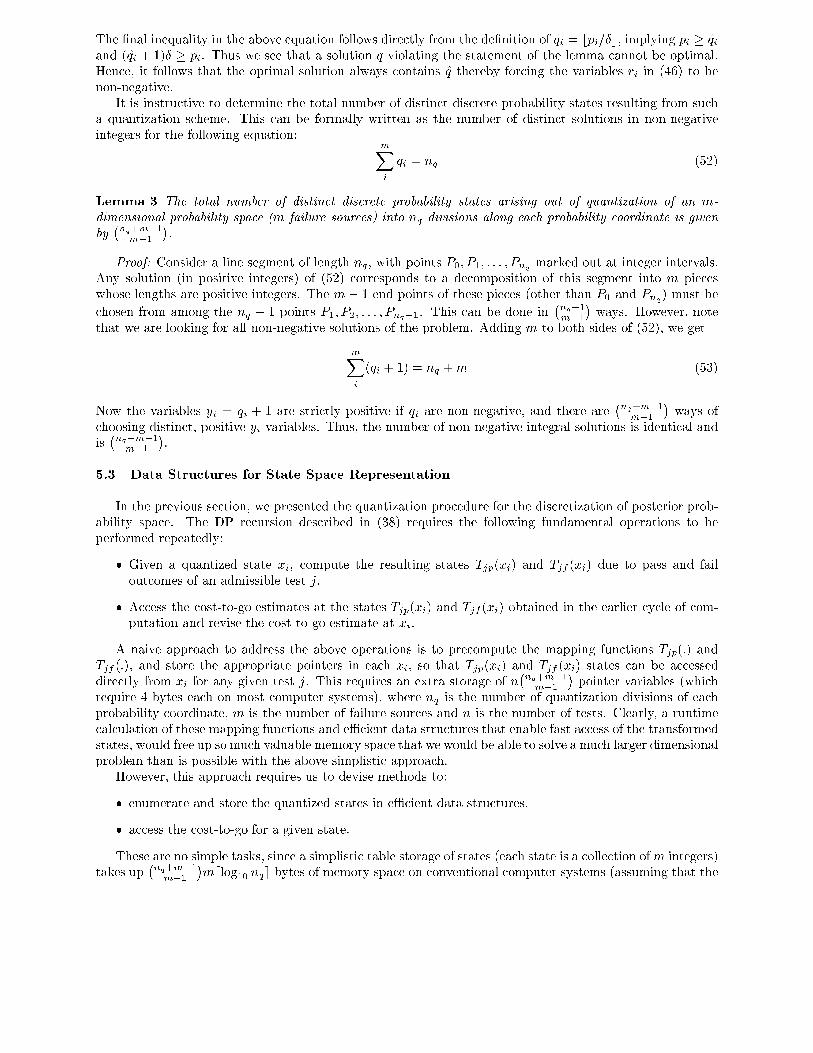
It is instru tive to determine the total number of distin t dis rete probability states resulting from su h
a quantization s heme. This an be formally written as the number of distin t solutions in non-negative
integers for the following equation:
m
X
i
q
i
= n
q
(52)
Lemma 3 The total number of distin t dis rete probability states arising out of quantization of an m-
dimensional probability spa e (m failure sour es) into n
q
divisions along ea h probability oordinate is given
by
�
n
q
+m�1
m�1
�
.
Proof: Consider a line segment of length n
q
, with points P
0
; P
1
; : : : ; P
n
q
marked out at integer intervals.
Any solution (in positive integers) of (52) orresponds to a de omposition of this segment into m pie es
whose lengths are positive integers. The m� 1 end points of these pie es (other than P
0
and P
n
q
) must be
hosen from among the n
q
� 1 points P
1
; P
2
; : : : ; P
n
q
�1
. This an be done in
�
n
q
�1
m�1
�
ways. However, note
that we are looking for all non-negative solutions of the problem. Adding m to both sides of (52), we get
m
X
i
(q
i
+ 1) = n
q
+m (53)
Now the variables y
i
= q
i
+ 1 are stri tly positive if q
i
are non-negative, and there are
�
n
q
+m�1
m�1
�
ways of
hoosing distin t, positive y
i
variables. Thus, the number of non-negative integral solutions is identi al and
is
�
n
q
+m�1
m�1
�
.
5.3 Data Stru tures for State Spa e Representation
In the previous se tion, we presented the quantization pro edure for the dis retization of posterior prob-
ability spa e. The DP re ursion des ribed in (38) requires the following fundamental operations to be
performed repeatedly:
� Given a quantized state x
i
, ompute the resulting states T
jp
(x
i
) and T
jf
(x
i
) due to pass and fail
out omes of an admissible test j.
� A ess the ost-to-go estimates at the states T
jp
(x
i
) and T
jf
(x
i
) obtained in the earlier y le of om-
putation and revise the ost-to-go estimate at x
i
.
A naive approa h to address the above operations is to pre ompute the mapping fun tions T
jp
(:) and
T
jf
(:), and store the appropriate pointers in ea h x
i
, so that T
jp
(x
i
) and T
jf
(x
i
) states an be a essed
dire tly from x
i
for any given test j. This requires an extra storage of n
�
n
q
+m�1
m�1
�
pointer variables (whi h
require 4 bytes ea h on most omputer systems), where n
q
is the number of quantization divisions of ea h
probability oordinate, m is the number of failure sour es and n is the number of tests. Clearly, a runtime
al ulation of these mapping fun tions and eÆ ient data stru tures that enable fast a ess of the transformed
states, would free up so mu h valuable memory spa e that we would be able to solve a mu h larger dimensional
problem than is possible with the above simplisti approa h.
However, this approa h requires us to devise methods to:
� enumerate and store the quantized states in eÆ ient data stru tures.
� a ess the ost-to-go for a given state.
These are no simple tasks, sin e a simplisti table storage of states (ea h state is a olle tion ofm integers)
takes up
�
n
q
+m�1
m�1
�
mdlog
10
n
q
e bytes of memory spa e on onventional omputer systems (assuming that the
Submitted to IEEE Trans. on Systems, Man, and Cyberneti s 12
integers are on atenated to form a string). And random a ess of a state in su h a table requires an average
of
�
n
q
+m�1
m�1
�
=2 omparisons.
In the following, we present a highly storage-eÆ ient, fast-a ess data stru ture tuned for this purpose.
We �rst need to introdu e some notation in order to give a formal des ription of the data stru tures involved.
Consider a dire ted graph T = (V;E) where, V is the set of verti es (nodes) and E is the set of edges. In
addition, let T be a dire ted rooted tree having one vertex whi h is the head of no edges ( alled the root)
and ea h vertex ex ept the root is the head of exa tly one edge. The relation (v; w) is an edge of T denoted
by v ! w. If v ! w, then v is termed parent of w and w is the hild of v. Let the fun tion d(v) represent
the depth of the node v in the rooted tree.
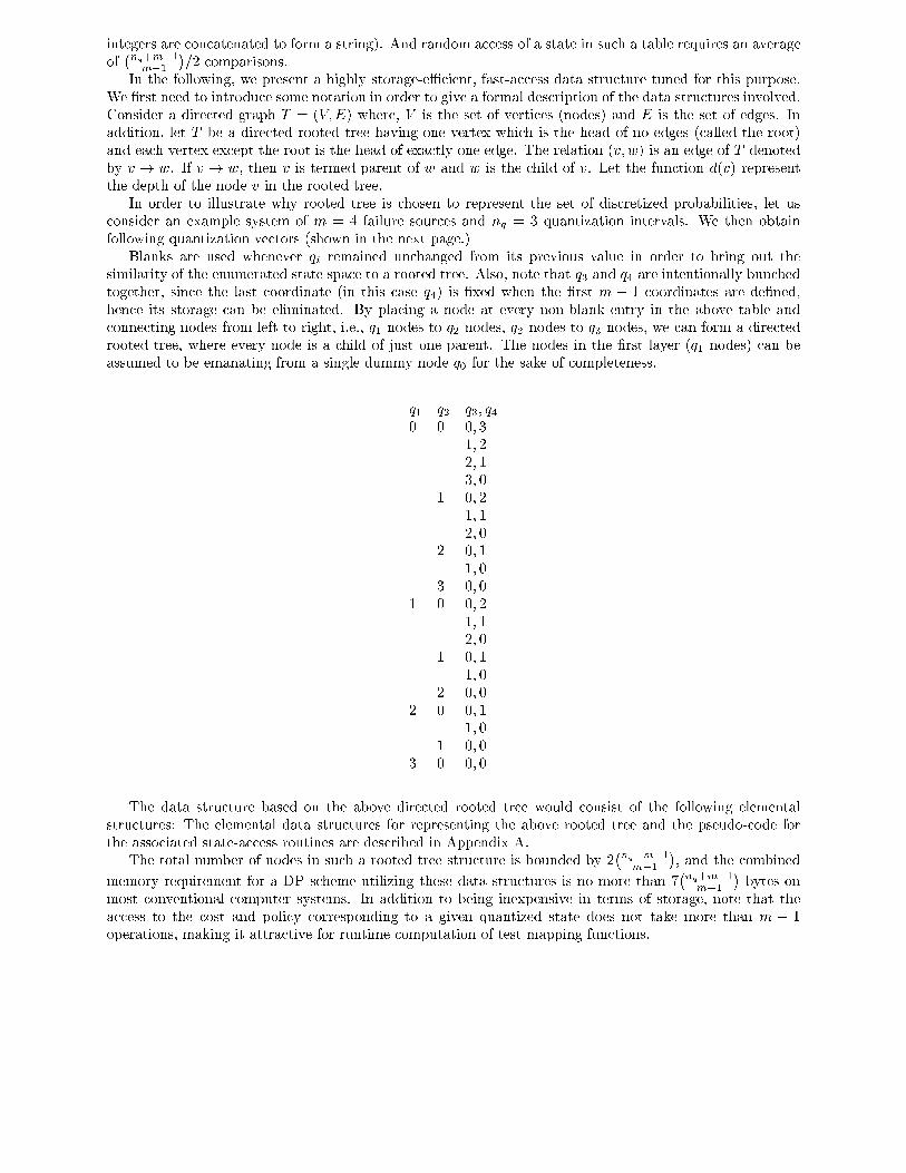
In order to illustrate why rooted tree is hosen to represent the set of dis retized probabilities, let us
onsider an example system of m = 4 failure sour es and n
q
= 3 quantization intervals. We then obtain
following quantization ve tors (shown in the next page.)
Blanks are used whenever q
i
remained un hanged from its previous value in order to bring out the
similarity of the enumerated state spa e to a rooted tree. Also, note that q
3
and q
4
are intentionally bun hed
together, sin e the last oordinate (in this ase q
4
) is �xed when the �rst m � 1 oordinates are de�ned,
hen e its storage an be eliminated. By pla ing a node at every non-blank entry in the above table and
onne ting nodes from left to right, i.e., q
1
nodes to q
2
nodes, q
2
nodes to q
3
nodes, we an form a dire ted
rooted tree, where every node is a hild of just one parent. The nodes in the �rst layer (q
1
nodes) an be
assumed to be emanating from a single dummy node q
0
for the sake of ompleteness.
q
1
q
2
q
3
; q
4
0 0 0; 3
1; 2
2; 1
3; 0
1 0; 2
1; 1
2; 0
2 0; 1
1; 0
3 0; 0
1 0 0; 2
1; 1
2; 0
1 0; 1
1; 0
2 0; 0
2 0 0; 1
1; 0
1 0; 0
3 0 0; 0
The data stru ture based on the above dire ted rooted tree would onsist of the following elemental
stru tures: The elemental data stru tures for representing the above rooted tree and the pseudo- ode for
the asso iated state-a ess routines are des ribed in Appendix A.
The total number of nodes in su h a rooted tree stru ture is bounded by 2
�
n
q
+m�1
m�1
�
, and the ombined
memory requirement for a DP s heme utilizing these data stru tures is no more than 7
�
n
q
+m�1
m�1
�
bytes on
most onventional omputer systems. In addition to being inexpensive in terms of storage, note that the
a ess to the ost and poli y orresponding to a given quantized state does not take more than m � 1
operations, making it attra tive for runtime omputation of test mapping fun tions.
Submitted to IEEE Trans. on Systems, Man, and Cyberneti s 13
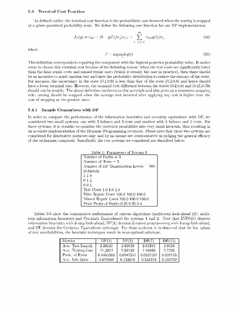
5.4 Terminal Cost Fun tion
As de�ned earlier, the terminal ost fun tion is the probabilisti ost in urred when the testing is stopped
at a given quantized probability state. We de�ne the following ost fun tion for our DP implementation:
J
T
(q) =
Ri
0
+ (1� q(i
0
)=n
q
)
Fi
0
+
m
X
i=1;i 6=i
0
Mi
q(i)=n
q
(54)
where
i
0
= argmax
i
q(i) (55)
This de�nition orresponds to repairing the omponent with the highest posterior probability value. It makes
sense to hoose this terminal ost be ause of the following reason: when the test osts are signi� antly lower
than the false repair osts and missed repair osts (whi h is usually the ase in pra ti e), then there should
be an in entive to apply another test and skew the probability distribution to redu e the entropy of the state.
For instan e, the un ertainty in the state (0.1,0.9) is less than that of the state (0.2,0.8) and hen e should
have a lower terminal ost. However, the terminal ost di�eren e between the states (0.2,0.8) and (0.21,0.79)
should not be sizable. The above de�nition onforms to this prin iple and also gives us a onsistent stopping
rule: testing should be stopped when the average ost in urred after applying any test is higher than the
ost of stopping at the present state.
5.4.1 Sample Comparison with DP
In order to ompare the performan e of the information heuristi s and ertainty equivalen e with DP, we
onsidered two small systems; one with 3 failures and 3 tests and another with 5 failures and 5 tests. For
these systems, it is possible to quantize the posterior proabilities into very small intervals, thus resulting in
an a urate implementation of the Dynami Programming re ursion. Please note that these two systems are
onsidered for illustrative purposes only and by no means are representative in judging the general eÆ a y
of the te hniques ompared. Spe i� ally the two systems we onsidered are des ribed below:
Table 1: Parameters of System 1
Number of Faults = 3
Number of Tests = 3
Number of DP Quantization Levels = 500
D-Matrix
1 1 0
0 1 1
0 0 1
Test Costs 1.0 1.0 1.0
False Repair Costs 100.0 100.0 100.0
Missed Repair Costs 100.0 100.0 100.0
Prior Probs of Faults 0.25 0.35 0.4
Tables 3-6 show the omparative performan e of various algorithms (multi-step look-ahead DP, multi-
step information heuristi s and Certainty Equivalen e) for systems 1 and 2. Note that INFO(k) denotes
information heuristi s with k-step look-ahead, DP(k) denotes dynami programming with k-step look-ahead,
and CE denotes the Certainty Equivalen e te hnique. For these systems, it is observed that for low values
of test unreliabilities, the heuristi te hniques result in near-optimal solutions.
Metri s DP(1) DP(3) DP(7) DP(15)
Ave. Test Length 2.29521 2.93849 2.94194 2.9416
Ave. Testing Cost 11.3974 7.88139 7.48886 7.1705
Prob. of Error 0.0455903 0.0247351 0.0227501 0.021155
Ave. Info Gain 0.678008 0.533618 0.534378 0.535792
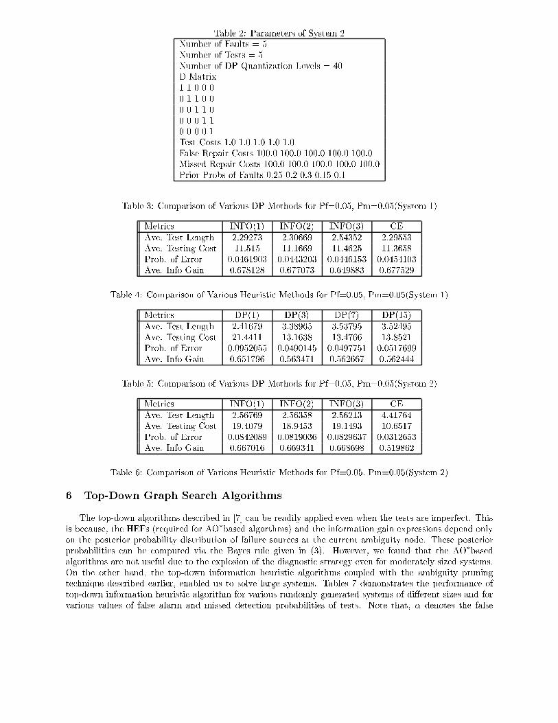
Submitted to IEEE Trans. on Systems, Man, and Cyberneti s 14
Table 2: Parameters of System 2
Number of Faults = 5
Number of Tests = 5
Number of DP Quantization Levels = 40
D-Matrix
1 1 0 0 0
0 1 1 0 0
0 0 1 1 0
0 0 0 1 1
0 0 0 0 1
Test Costs 1.0 1.0 1.0 1.0 1.0
False Repair Costs 100.0 100.0 100.0 100.0 100.0
Missed Repair Costs 100.0 100.0 100.0 100.0 100.0
Prior Probs of Faults 0.25 0.2 0.3 0.15 0.1
Table 3: Comparison of Various DP Methods for Pf=0.05, Pm=0.05(System 1)
Metri s INFO(1) INFO(2) INFO(3) CE
Ave. Test Length 2.29273 2.30669 2.54352 2.29553
Ave. Testing Cost 11.515 11.1669 11.4625 11.3658
Prob. of Error 0.0461903 0.0443203 0.0446153 0.0454103
Ave. Info Gain 0.678128 0.677073 0.649883 0.677529
Table 4: Comparison of Various Heuristi Methods for Pf=0.05, Pm=0.05(System 1)
Metri s DP(1) DP(3) DP(7) DP(15)
Ave. Test Length 2.41679 3.38965 3.53795 3.52495
Ave. Testing Cost 21.4411 13.1638 13.4766 13.8521
Prob. of Error 0.0952055 0.0490145 0.0497751 0.0517699
Ave. Info Gain 0.651796 0.563471 0.562667 0.562444
Table 5: Comparison of Various DP Methods for Pf=0.05, Pm=0.05(System 2)
Metri s INFO(1) INFO(2) INFO(3) CE
Ave. Test Length 2.56769 2.56358 2.56213 4.41764
Ave. Testing Cost 19.4079 18.9453 19.1493 10.6517
Prob. of Error 0.0842089 0.0819036 0.0829637 0.0312653
Ave. Info Gain 0.667016 0.669341 0.668698 0.519862
Table 6: Comparison of Various Heuristi Methods for Pf=0.05, Pm=0.05(System 2)
6 Top-Down Graph Sear h Algorithms
The top-down algorithms des ribed in [7℄ an be readily applied even when the tests are imperfe t. This
is be ause, the HEFs (required for AO
�
based algorthms) and the information gain expressions depend only
on the posterior probability distribution of failure sour es at the urrent ambiguity node. These posterior
probabilities an be omputed via the Bayes rule given in (3). However, we found that the AO
�
based
algorithms are not useful due to the explosion of the diagnosti strategy even for moderately sized systems.
On the other hand, the top-down information heuristi algorithms oupled with the ambiguity pruning
te hnique des ribed earlier, enabled us to solve large systems. Tables 7 demonstrates the performan e of
top-down information heuristi algorithm for various randomly generated systems of di�erent sizes and for
various values of false alarm and missed dete tion probabilities of tests. Note that, � denotes the false
Submitted to IEEE Trans. on Systems, Man, and Cyberneti s 15
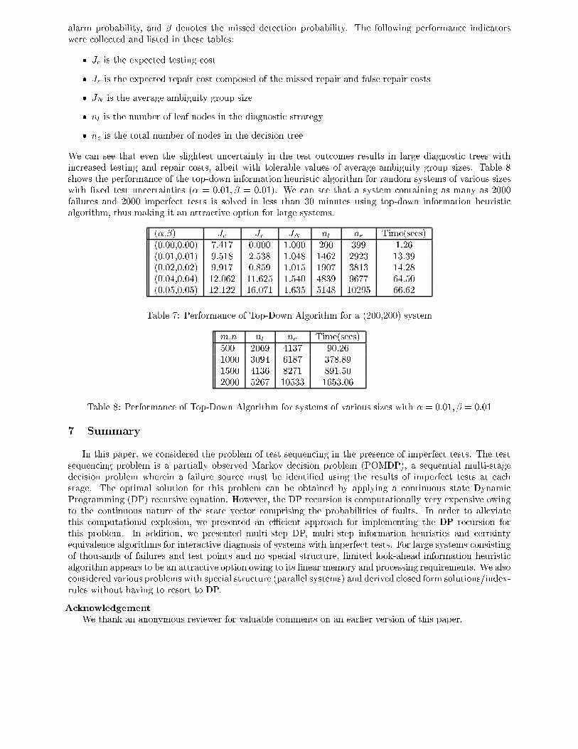
alarm probability, and � denotes the missed dete tion probability. The following performan e indi ators
were olle ted and listed in these tables:
� J
is the expe ted testing ost
� J
r
is the expe ted repair ost omposed of the missed repair and false repair osts
� J
N
is the average ambiguity group size
� n
l
is the number of leaf nodes in the diagnosti strategy
� n
e
is the total number of nodes in the de ision tree
We an see that even the slightest un ertainty in the test out omes results in large diagnosti trees with
in reased testing and repair osts, albeit with tolerable values of average ambiguity group sizes. Table 8
shows the performan e of the top-down information heuristi algorithm for random systems of various sizes
with �xed test un ertainties (� = 0:01; � = 0:01). We an see that a system ontaining as many as 2000
failures and 2000 imperfe t tests is solved in less than 30 minutes using top-down information heuristi
algorithm, thus making it an attra tive option for large systems.
(�,�) J
J
r
J
N
n
l
n
e
Time(se s)
(0.00,0.00) 7.417 0.000 1.000 200 399 1.26
(0.01,0.01) 9.518 2.538 1.048 1462 2923 13.39
(0.02,0.02) 9.917 0.859 1.015 1907 3813 14.28
(0.04,0.04) 12.062 11.625 1.540 4839 9677 64.50
(0.05,0.05) 12.122 16.071 1.635 5148 10295 66.62
Table 7: Performan e of Top-Down Algorithm for a (200,200) system
m,n n
l
n
e
Time(se s)
500 2069 4137 90.26
1000 3094 6187 378.89
1500 4136 8271 891.50
2000 5267 10533 1653.06
Table 8: Performan e of Top-Down Algorithm for systems of various sizes with � = 0:01; � = 0:01
7 Summary
In this paper, we onsidered the problem of test sequen ing in the presen e of imperfe t tests. The test
sequen ing problem is a partially observed Markov de ision problem (POMDP), a sequential multi-stage
de ision problem wherein a failure sour e must be identi�ed using the results of imperfe t tests at ea h
stage. The optimal solution for this problem an be obtained by applying a ontinuous state Dynami
Programming (DP) re ursive equation. However, the DP re ursion is omputationally very expensive owing
to the ontinuous nature of the state ve tor omprising the probabilities of faults. In order to alleviate
this omputational explosion, we presented an eÆ ient approa h for implementing the DP re ursion for
this problem. In addition, we presented multi-step DP, multi-step information heuristi s and ertainty
equivalen e algorithms for intera tive diagnosis of systems with imperfe t tests. For large systems onsisting
of thousands of failures and test points and no spe ial stru ture, limited look-ahead information heuristi
algorithm appears to be an attra tive option owing to its linear memory and pro essing requirements. We also
onsidered various problems with spe ial stru ture (parallel systems) and derived losed form solutions/index-
rules without having to resort to DP.
A knowledgement
We thank an anonymous reviewer for valuable omments on an earlier version of this paper.
Submitted to IEEE Trans. on Systems, Man, and Cyberneti s 16
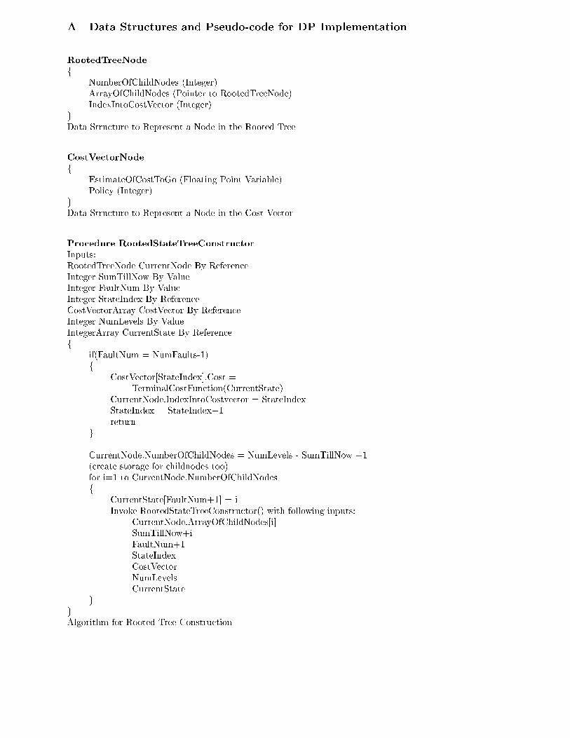
A Data Stru tures and Pseudo- ode for DP Implementation
RootedTreeNode
f
NumberOfChildNodes (Integer)
ArrayOfChildNodes (Pointer to RootedTreeNode)
IndexIntoCostVe tor (Integer)
g
Data Stru ture to Represent a Node in the Rooted Tree
CostVe torNode
f
EstimateOfCostToGo (Floating Point Variable)
Poli y (Integer)
g
Data Stru ture to Represent a Node in the Cost Ve tor
Pro edure RootedStateTreeConstru tor
Inputs:
RootedTreeNode CurrentNode By Referen e
Integer SumTillNow By Value
Integer FaultNum By Value
Integer StateIndex By Referen e
CostVe torArray CostVe tor By Referen e
Integer NumLevels By Value
IntegerArray CurrentState By Referen e
f
if(FaultNum = NumFaults-1)
f
CostVe tor[StateIndex℄.Cost =
TerminalCostFun tion(CurrentState)
CurrentNode.IndexIntoCostve tor = StateIndex
StateIndex = StateIndex+1
return
g
CurrentNode.NumberOfChildNodes = NumLevels - SumTillNow +1
( reate storage for hildnodes too)
for i=1 to CurrentNode.NumberOfChildNodes
f
CurrentState[FaultNum+1℄ = i
Invoke RootedStateTreeConstru tor() with following inputs:
CurrentNode.ArrayOfChildNodes[i℄
SumTillNow+i
FaultNum+1
StateIndex
CostVe tor
NumLevels
CurrentState
g
g
Algorithm for Rooted Tree Constru tion
Submitted to IEEE Trans. on Systems, Man, and Cyberneti s 17
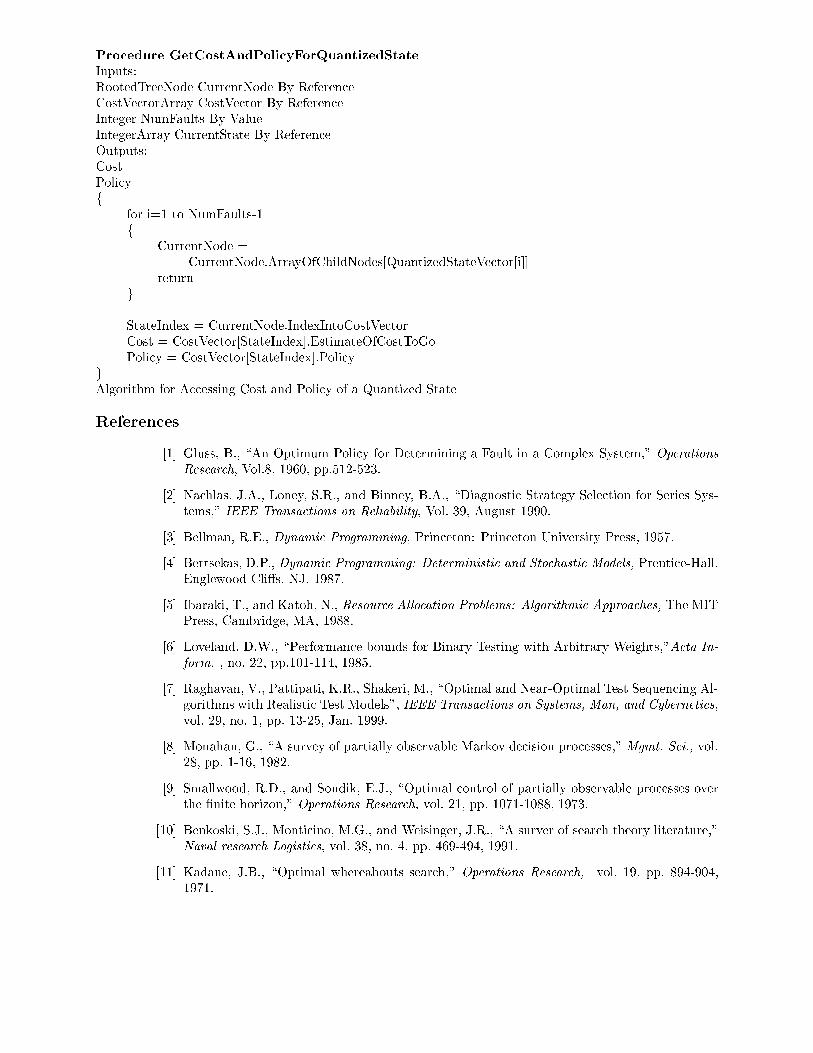
Pro edure GetCostAndPoli yForQuantizedState
Inputs:
RootedTreeNode CurrentNode By Referen e
CostVe torArray CostVe tor By Referen e
Integer NumFaults By Value
IntegerArray CurrentState By Referen e
Outputs:
Cost
Poli y
f
for i=1 to NumFaults-1
f
CurrentNode =
CurrentNode.ArrayOfChildNodes[QuantizedStateVe tor[i℄℄
return
g
StateIndex = CurrentNode.IndexIntoCostVe tor
Cost = CostVe tor[StateIndex℄.EstimateOfCostToGo
Poli y = CostVe tor[StateIndex℄.Poli y
g
Algorithm for A essing Cost and Poli y of a Quantized State
Referen es
[1℄ Gluss, B., \An Optimum Poli y for Determining a Fault in a Complex System," Operations
Resear h, Vol.8, 1960, pp.512-523.
[2℄ Na hlas, J.A., Loney, S.R., and Binney, B.A., \Diagnosti Strategy Sele tion for Series Sys-
tems," IEEE Transa tions on Reliability, Vol. 39, August 1990.
[3℄ Bellman, R.E., Dynami Programming, Prin eton: Prin eton University Press, 1957.
[4℄ Bertsekas, D.P., Dynami Programming: Deterministi and Sto hasti Models, Prenti e-Hall,
Englewood Cli�s, NJ, 1987.
[5℄ Ibaraki, T., and Katoh, N., Resour e Allo ation Problems: Algorithmi Approa hes, The MIT
Press, Cambridge, MA, 1988.
[6℄ Loveland, D.W., \Performan e bounds for Binary Testing with Arbitrary Weights,"A ta In-
form. , no. 22, pp.101-114, 1985.
[7℄ Raghavan, V., Pattipati, K.R., Shakeri, M., \Optimal and Near-Optimal Test Sequen ing Al-
gorithms with Realisti Test Models", IEEE Transa tions on Systems, Man, and Cyberneti s,
vol. 29, no. 1, pp. 13-25, Jan. 1999.
[8℄ Monahan, G., \A survey of partially observable Markov de ision pro esses," Mgmt. S i., vol.
28, pp. 1-16, 1982.
[9℄ Smallwood, R.D., and Sondik, E.J., \Optimal ontrol of partially observable pro esses over
the �nite horizon," Operations Resear h, vol. 21, pp. 1071-1088, 1973.
[10℄ Benkoski, S.J., Monti ino, M.G., and Weisinger, J.R., \A surver of sear h theory literature,"
Naval resear h Logisti s, vol. 38, no. 4, pp. 469-494, 1991.
[11℄ Kadane, J.B., \Optimal whereabouts sear h," Operations Resear h, vol. 19, pp. 894-904,
1971.
Submitted to IEEE Trans. on Systems, Man, and Cyberneti s 18
[12℄ Tognetti, K.P., \An optimal strategy for whereabouts sear h," Operations Resear h, vol. 16,
pp. 209-211, 1968.
[13℄ Raghavan, V., Willett, P., Pattipati, K., Kleinman, D., \Optimal measurement sequen ing in
M-ary hypothesis testing problems," in Pro . 1992 Ameri an Control Conferen e, Chi ago,
IL, June 1992.
[14℄ Sheridan, T.B., \On how often a supervisor shoudl sample," IEEE Trans. Syst. Man Cyber.,
vol. 13, no. 1, pp. 37-46, Jan/Feb 1965.
[15℄ Dobbie, J.M., \Some sear h problems with false onta s," Operations Resear h, vol. 21, pp.
907-925, 1973.
[16℄ Stone, L.D., and Stanshine, J.A., \Optimal sear h using uninterrupted onta t investigation,"
SIAM J. Appl. Math., vol. 20, pp. 241-263, 1971.
[17℄ Stone, L.D., and Stanshine, J.A., \Optimal sear h in the presen e of poisson-distributed false
targets," SIAM J. Appl. Math., vol. 23, pp. 6-27, 1972.
[18℄ Wald, A., Sequential Analysis, New York: John Wiley, 1947.


