When is Information Sufficient for Action? Search with

Unreliable Yet Informative Intelligence

Michael P. Atkinson∗, Moshe Kress†, Rutger-Jan Lange‡

January 12, 2016

Abstract

We analyze a variant of the whereabouts search problem, in which a searcher looks

for a target hiding in one of n possible locations. Unlike in the classic version, our

searcher does not pursue the target by actively moving from one location to the next.

Instead, the searcher receives a stream of intelligence about the location of the target.

At any time, the searcher can engage the location he thinks contains the target or wait

for more intelligence. The searcher incurs costs when he engages the wrong location,

based on insufficient intelligence, or waits too long in the hopes of gaining better sit-

uational awareness, which allows the target to either execute his plot or disappear.

We formulate the searcher’s decision as an optimal stopping problem and establish

conditions for optimally executing this search-and-interdict mission.

Keywords : whereabouts search, optimal stopping, multinomial selection

∗mpatkins@nps.edu Operations Research Department, Naval Postgraduate School†mkress@nps.edu Operations Research Department, Naval Postgraduate School‡rutger-jan.lange@cantab.net Finance Department, VU University Amsterdam & School of Economics,

Erasmus University Rotterdam

1

1 Introduction

Operation Neptune Spear led to the capture and elimination of Osama bin Laden by the US

in 2011. While US intelligence agencies had continuously collected information regarding his

whereabouts, the dilemma was when to act. Raiding a wrong location, based on insufficient or

false information, would cause collateral damage, diplomatic blowback and loss of intelligence

assets. On the other hand, waiting too long for more information could result in bin Laden

escaping. The dilemma between “act now” or “wait and see” was acute but fortunately was

resolved successfully in this case. Another example of such a dilemma concerns a “ticking

bomb” scenario (Kaplan, 2012). In this scenario a hiding terrorist plots to attack a target

(e.g., a suicide bomber), and the authorities must race to stop the attack. A final example

involves an operation to rescue hostages held by an insurgency group. The insurgents may

kill the hostages (e.g., in an escape attempt) if the authorities delay the operation for too

long. However, a failed rescue attempt may alert the insurgents resulting in the deaths of

the hostages. Many military, law enforcement, and intelligence investigations face a similar

tradeoff decision concerning timing and cost of premature action.

Motivated by the aforementioned examples, we consider a search situation called the

whereabouts search problem (Kadane, 1971; Stone, 1975). In its simplest form, a target lies

hidden in one of n cells, where pi is the probability that the target resides in cell i,∑n

i=1 pi = 1,

and ci is the cost of searching cell i. The searcher examines one cell at a time and the search

is error-free; if a cell contains the target, the searcher will detect it. The objective is to find a

search strategy – an order in which to search the cells – to minimize the expected total search

cost. Several variations of this problem include, among others, situations where a search is

subject to error (Kress et al., 2008; Wilson et al., 2011), the target moves (Komiya et al.,

2006) or acts strategically (An et al., 2013) , and multiple targets arrive and disappear in a

random fashion (Szechtman et al., 2008). However, all of the aforementioned cases share the

same definition of a strategy, namely, a search sequence for an active searcher.

In this paper, we consider the same physical description of the whereabouts problem: a

2

single static target hidden in one of n cells. However, the operational setting is different in

two major aspects: (a) the searcher does not actively search the cells but instead relies on

occasional pieces of intelligence of the form “cell i contains the target”, and (b) the search

mission is time-critical. The searcher does not control the arrival rate of intelligence, and an

intelligence item may be wrong. At a certain point the searcher may choose a cell to engage

in the hope of interdicting the target. If the searcher chooses the wrong cell, he incurs a cost

comprising collateral damage, loss of intelligence assets, political ramifications, etc.

We describe the problem in Section 2 and formulate the mathematical model in Section 3.

The cases of n = 2 and n =∞ appear in Sections 4 and 5, respectively. Section 6 examines

the optimal strategy when 2 < n < ∞. We present numerical illustrations in Section 7.

Section 8 discusses extensions. All proofs appear in the Appendix.

2 The Problem

A searcher wants to interdict a target, residing in one of n possible cells, before some event

occurs. Such an event would be, for example, the disappearance of bin Laden from a certain

region or an execution of a terror plot, which we use as our reference scenario. An attack

occurs when the plot fully matures, and the plotting time is exponentially distributed with

mean 1/µ (a similar assumption appears in Kaplan (2010)). While the searcher may have

some initial notion regarding the target’s location based on exogenous intelligence, we will

often focus on the case where there is none: the uniform prior location distribution.

Independent intelligence items from human informants, intercepted communications and

interrogations of the form “cell i contains the target” arrive according to a Poisson process

with rate λ. The searcher has no control over the timing or content of the items. Thus,

scheduled sensor cues (e.g., RADAR, SONAR, images, videos) from cells do not apply here.

Although our model applies to a variety of intelligence sources, we use, as a reference setting,

human informants who provide tips. For most of our analysis the parameters µ and λ only

3

appear via the intensity ratio ρ = µ/λ.

If, following a certain number of tips, the searcher decides to engage a specific cell, the

search ends, even if the searcher chooses incorrectly. If the searcher engages the correct cell,

the target is interdicted. However, if the searcher engages the wrong cell, then the target

realizes that he is being hunted, and therefore immediately executes his (not fully mature)

plot before the searcher finds him. In Section 8.1 we consider a variant where the target only

executes mature plots and the searcher continues obtaining intelligence and engaging cells

until he either finds the target or the target attacks.

The searcher desires to minimize the expected cost of two possible negative outcomes: (a)

engaging a wrong cell, or (b) execution of a mature attack by the target. The costs of (a) and

(b) are c and d, respectively. The false positive cost c comprises collateral damage resulting

from engaging an innocent cell and the (possible) cost of a premature attack. We neither

need nor make any assumption regarding the relative values of c and d. Because the results

to follow only depend on the the cost-ratio α = d/c, we assume, without loss of generality,

that c = 1 and d = α.

A tip specifies the correct cell with probability q. We often refer to q as the informant’s

reliability. Informants are neither clueless nor malevolent, that is, q > 1n. If the informant

provides an incorrect tip (with probability 1 − q), then the error is uniform; the informant

specifies each one of the n− 1 incorrect cells with equal probability.

The question is: when should the searcher engage a cell? We have here a “race” between

the flow of tips and the time of attack. On the one hand, the searcher wants to receive as

many tips as possible to reduce his uncertainty about the target’s location. On the other

hand, this “wait and see” approach may lead to the target attacking before the searcher has

the chance to do so. If the searcher instead rushes to engage a cell, the likelihood of a false

positive error increases. The searcher knows the values of all the parameters involved in this

process: n, q, α, and ρ.

This search problem is an example of an optimal stopping problem (Chow et al., 1971;

4

Shiryaev, 2007; Ferguson, 2004). Wald and Wolfowitz (1948) examine a similar problem in

their work on the sequential probability ratio test. They show that the decision between se-

lecting a hypothesis and receiving another observation is optimally determined by a threshold

policy. In our model, when n = 2 cells, we find a similar threshold result (see Section 4),

which does not hold for n > 2. For n > 2, our problem can be framed as a higher dimensional

stopping problem. Lange (2012) examines optimal stopping of an n-dimensional Brownian

motion, and shows that the continuation region is generally also n-dimensional. While stan-

dard one-dimensional techniques do not apply, he shows that the continuation region can be

found by reformulating the problem as a free-boundary problem in n dimensions.

When n > 2 cells, our problem relates to the family of multinomial selection problems

(Kim and Nelson, 2006) in which an observation specifies the “winner” among n competing

alternatives. A decision maker may either observe a fixed number of samples before choosing

the best option (Bechhofer et al., 1959) or may dynamically decide, after each observation,

whether to pick an alternative or receive another observation (Ramey and Alam, 1979).

Most formulations desire to achieve a lower bound on the probability of choosing the correct

alternative, provided certain conditions about the system hold. These conditions usually

relate to the relationship between the true probabilities of the two best alternatives (Chen,

1988). A good survey of the techniques used in multinomial selection problems appears in

Vieira et al. (2014). Most selection problems assume a deterministic number of observations.

In our problem the number of tips is random because the time until the plot matures is

random. We found only two multinomial selection papers that examine a random maximum

number of observations (Frazier and Yu, 2007; Dayanik and Yu, 2013). The model in Frazier

and Yu (2007) considers only the n = 2 case and allows for a general stochastic deadline,

which is analogous to the time until the attack occurs in our model. The approach in Dayanik

and Yu (2013) does allow for n > 2 alternatives. It focuses on neuroscience applications and

considers a cost-rate, as opposed to total cost in our model.

Finally, note that our model has one decision maker, the searcher. One could view the

5

problem as having three strategic players: the searcher, the target, and the informant. We

consider here a simpler, yet, we believe, a realistic situation where the target does not really

know the searcher’s operational options and the informant is incentivized by the searcher to

do the best he can. One could develop a two-player Markov game between the searcher and

target similar to the Inspection Game (see Chapter 4 of Washburn (2014)). However, the

formulation would quickly become unwieldy because one would need to specify not only the

intelligence picture of each player, but also each player’s perceived intelligence picture.

3 Mathematical Preliminaries

The decision to engage a cell or wait for more tips depends on the expected cost of each option.

In this section we develop the mathematical building blocks to compute these expected

costs. Two factors determining the expected costs are Location probability, which specifies

the likelihood that cell i contains the target, and Pointing probability that specifies the

likelihood that the next tip points at cell i. In Section 3.1 we compute these probabilities,

and in Section 3.2 we use these probabilities to derive the expected costs.

3.1 Location and Pointing Probabilities

Let p = (p1, ..., pn) denote the current location probabilities and let p denote the initial

location probabilities, before the first tip. Let si be the number of tips thus far specifying cell

i as the target’s location, and s = (s1, ..., sn). In this subsection we assume that s1 ≥ ... ≥ sn.

The location probability of cell i given s is:

pi(s) = P[target in i | s] =P[s | target in i]pi∑nj=1 P[s | target in j]pj

. (1)

6

An informant points to the correct cell with probability q and a specific incorrect cell with

probability 1−qn−1 . Thus, utilizing the multinomial nature of s, we have

P[s | target in i] =(∑

k sk)!∏k sk!

qsi(

1− qn− 1

)∑k 6=i sk

=(∑

k sk)!∏k sk!

(1− qn− 1

)∑nk=1 sk

(q

1−qn−1

)si

=(∑

k sk)!∏k sk!

(1− qn− 1

)∑nk=1 sk

γsi , (2)

where

γ =q

1−qn−1

. (3)

Note that only the γsi portion of (2) depends on i. This is a direct consequence of our

assumption that each wrong cell is equal likely to be pointed at. When we substitute (2)

back into (1), most terms cancel, and the location probability simplifies to:

pi(s) =γsi pi∑nj=1 γ

sj pj. (4)

Note from equation (4) that pi(s) is invariant to additive shifts in s. If s is such that si = si+L

for some integer L, then pi(s) = pi(s). Specifically, if we set L = −sn = −min(s) and use

si = si − sn, then we can write si =∑n−1

j=i ∆j, where ∆j = sj − sj+1 ≥ 0. Therefore, pi(s) is

uniquely determined by the tip-differentials ∆j, j = 1, ..., n− 1.

While s or ∆ are natural state vectors, it is simpler to use the location probabilities

p = (p1, ..., pn) as the state vector for most of the mathematical analysis in Sections 4–6.

7

Specifically, if the next tip points to cell i, then the updated probability p(+i)j for cell j is:

p(+i)j =

γpi

γpi+(1−pi) if j = i

pjγpi+(1−pi) if j 6= i.

(5)

Recall that according to our assumption q > 1n

and therefore γ > 1. Consequently, a tip

pointing to cell i increases the posterior location probability of cell i (p(+i)i ≥ pi) and decreases

the posterior probability of other cells (p(+i)j ≤ pj for j 6= i).

We next define B(p) as the set of cells with the highest location probability:

B(p) = {i : pi = maxjpj, 1 ≤ i ≤ n}. (6)

The following proposition defines a lower bound on maxj pj . The proof appears in Appendix

A.

Proposition 1. If |B(p)| = 1 and the prior distribution for the target’s location is uniform,

then maxj pj ≥ q.

Next we consider the pointing probability ri(p) that the next tip points to cell i, given

the current location probabilities p:

ri(p) ≡ P[informant says i | p] =n∑k=1

P[informant says i | p, target in k]P[target in k | p]

= qpi +1− qn− 1

∑k 6=i

pk = qpi +1− qn− 1

(1− pi). (7)

Inspection of (7) reveals that ri(p) ∈ [ 1−qn−1 , q]. Thus, a tip may point at a cell other than i,

even if pi is close to 1, if q << 1. Note also that ri(p) only depends on pi, it does not depend

upon how the remaining (1− pi) probability mass is spread among the other n− 1 cells.

8

3.2 Expected Cost

Define C(p) as the expected cost if the searcher acts optimally in state p. Since an optimal

stopping problem is a dynamic programming problem (Chow et al., 1971), we compute C(p)

by comparing the expected costs of two decisions: engage or wait. That is,

C(p) = min

(expected cost if the searcher engages a cell,

ρ

1 + ρα +

1

1 + ρexpected cost after receiving the next tip

). (8)

If the searcher decides to wait, the target may attack before the searcher receives the next

tip. In that case, which happens with probability ρ1+ρ

, the mature attack produces a cost of

α. If the next tip arrives before the target’s attack, the system transitions, and we assume

the searcher behaves optimally in the future. Next we compute the expected costs of the two

possible options: engage or wait.

If the searcher decides to engage cell j while in state p, the expected cost is 1 − pj.

Obviously, the searcher should engage a cell in B(p); the searcher can use any tie-breaking

mechanism if B(p) contains multiple cells. To simplify notation, we henceforth assume,

without loss of generality, that p1 ≥ ... ≥ pn. Therefore B(p) contains cell 1 and

E[Cost if searcher decides to engage | p] = 1−maxjpj = 1− p1. (9)

If the searcher decides to wait, and an informant next points to cell i, then p transitions to

p(+i) according to equation (5). The informant points to cell i with probability ri(p), and the

searcher will incur an expected cost of C(p(+i)) if this occurs. Putting these pieces together,

9

we have

E[Cost if waiting for and receiving the next tip | p] =n∑i=1

P[informant says i | p]C(p(+i))

=n∑i=1

ri(p)C(p(+i)). (10)

Moving to the general case, we combine equations (8), (9), and (10) to produce the

complete cost function:

C(p) = min

(1− p1,

ρ

1 + ρα +

1

1 + ρ

n∑i=1

ri(p)C(p(+i))

). (11)

If the searcher is indifferent between engaging and waiting, he engages. In Appendix B

we present characteristics of C(p), such as its concavity. As most of these results are fairly

intuitive (e.g., C(p) decreases if the informant next points to cell 1), we defer this discussion

to the Appendix.

4 The Case of Two Cells

Arguably, the simpler the form of the optimal policy the more attractive it is operationally.

One such simple form is a threshold policy: the searcher engages if and only if p1 ≥ τ for some

threshold τ (recall we assume that p1 ≥ p2). The next corollary follows from the convexity

of the engage region (see Proposition EC.2 in Appendix B).

Corollary 1. For n = 2, the searcher should engage if and only if p1 ≥ τ for some threshold

τ ∈ [0.5, 1).

We prove this corollary in Appendix C. While there is an explicit expression for the thresh-

old τ , its derivation is cumbersome and therefore we defer most of its details to Appendix D.

10

A necessary and sufficient condition to engage in all states (i.e., τ = 0.5) is

1

2≥ ρ

1 + ρ(1− α) +

1

1 + ρq. (12)

If condition (12) does not hold then τ > 0.5. See Appendix D for the general expression for

τ when τ > 0.5. The implication is straightforward; if damage from a mature attack exceeds

the false positive cost (α ≥ 1) and the informant has low reliability (q ≈ 0.5), the searcher

should always engage. The benefits from future tips are small, and the risk of waiting is high.

To derive τ we leverage off the rich results related to the gambler’s ruin problem. Denote

p as the the prior state before the arrival of the s1+ s2 tips. Using equation (4) we transform

p to p :

p1 =γs1 p1

γs1 p1 + γs2(1− p1)=

γs1−s2 p1γs1−s2 p1 + (1− p1)

(13)

p2 =γs2(1− p1)

γs1 p1 + γs2(1− p1)=

1− p1γs1−s2 p1 + (1− p1)

. (14)

To update the probabilities we only need to know the tip-differential s1 − s2. We model

∆ ≡ s1−s2 as a random walk. For a given prior p, we can transform the threshold policy from

the real number τ to two non-negative integers A(p, τ) and B(p, τ) such that the searcher

waits as long as −B(p, τ) < ∆ < A(p, τ). If ∆ first hits A(p, τ) (−B(p, τ)), the searcher

engages cell 1 (cell 2). This approach facilitates the use of gambler’s ruin machinery to

compute relevant parameters (See Appendix D for details).

It is difficult to gain much insight about the optimal threshold τ using purely analytic

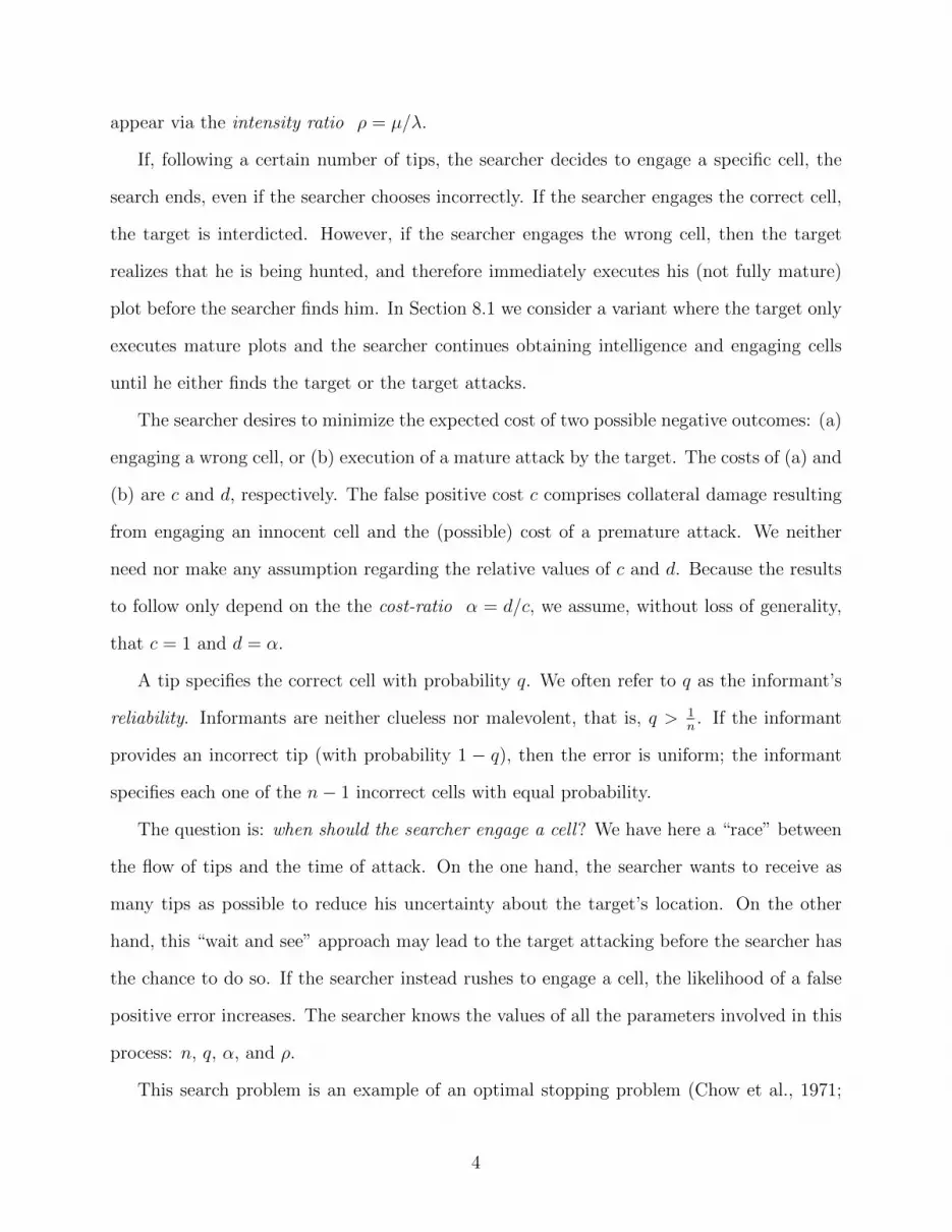
approaches. Thus, we illustrate its behavior using several figures. Figure 1 presents how the

threshold τ varies with informant reliability q for fixed cost-ratio α and intensity-ratio ρ. As

we move from Figure 1a to Figure 1c, we increase α from 0.5 to 2. Each curve on a figure

corresponds to a fixed value of ρ ∈ {0.01, 0.1, 1}. The threshold τ is a non-decreasing function

of q. A more reliable informant reduces the engage region and makes the searcher more likely

to wait because future tips are more valuable. The threshold decreases as we increase either

11

α (mature attack becomes more costly) or ρ (mature attack becomes more imminent) and

hence the engage region expands. In particular, in some situations with large α and/or large

ρ, the searcher immediately engages regardless of the current state p or informant reliability

q.

(a) α = 0.5 (b) α = 1 (c) α = 2

Figure 1: Engage threshold τ as a function of q for fixed combinations of ρ ∈ {0.01, 0.1, 1}and α ∈ {0.5, 1, 2}.

An interesting phenomenon relates to the expected number of tips received by the searcher

when acting optimally. One would expect that this number will decrease as the informant

becomes more reliable and therefore the searcher can reach the engage decision faster. Figure

2 demonstrates that this is not always the case. See Appendix E for the derivation of the

expected number of tips. Assuming the search starts in the uniform state p = (0.5, 0.5),

Figures 2b and 2c show that if ρ is small (the inflow rate of tips is much larger than the

attack rate) it is possible that the expected number of tips actually increases with q when the

latter is small enough. This non-monotonicity results from two conflicting factors. On one

hand, as q increases the threshold increases (see Figure 1), which suggests that the searcher

may need more tips to reach the threshold. On the other hand, a larger q implies that the

informant will point to the correct cell more frequently, which suggests that the searcher will

reach the threshold following fewer tips. Specifically, for q ≈ 1, the searcher will only need

one tip. In general, the first or second factor may dominate depending upon the values of α,

ρ, q. In most cases, when ρ is relatively large, the imminent attack dictates a swift action by

the searcher, as shown in the dashed and –◦– curves, which are close to 0.

12

The jumps in Figure 2 occur when the optimal tip-differential changes by 1. For a

fixed optimal tip-differential, the expected number of tips decreases as q increases because a

more reliable informant will produce a stream of tips that reaches that tip-differential faster

(probabilistically) than a less reliable informant.

(a) α = 0.5 (b) α = 1 (c) α = 2

Figure 2: Expected number of tips, starting from the uniform state p = (0.5, 0.5), until thesearch ends as a function of q for fixed combinations of ρ ∈ {0.01, 0.1, 1} and α ∈ {0.5, 1, 2}.The search ends either when the searcher engages or when a mature attack occurs.

5 The Case of an Infinite Number of Cells

When n is very large and the cells are equally likely to contain the target, it is unlikely that

the informant will point to the same incorrect cell twice. Thus, a second tip to the same

cell should indicate that it is the correct one. In Appendix F.1 we make this argument more

rigorous. If n =∞ and the informant points twice to the same cell, then the searcher knows

with certainty that this cell contains the target. We refer to the second tip to the same cell

as the confirming tip. In Appendix F.2 we derive the optimal policy, which we summarize in

the next Proposition.

Proposition 2. The searcher will choose the lowest cost alternative among the following

three options

1. Immediately engage any cell before receiving the first tip: cost is 1

2. Obtain one tip and engage the corresponding cell: cost is ρ1+ρ

α + 11+ρ

(1− q);

13

3. Wait for the confirming tip and then engage: cost is α

(1−

(qρ+q

)2).

Thus, the searcher should

choose option 1 iff α > 1 +q

ρ,

choose option 3 iff α < 1 +q

ρ

q − ρ2 − ρq − q2

ρ+ 2q − q2,

choose option 2 otherwise.

The searcher causes collateral damage if he chooses option 1 because he engages the

wrong cell. The cost for option 2 follows immediately from (11) as p1 = q after the tip. If

the searcher chooses option 3, there is no collateral damage, but the target may execute the

attack before confirming tip arrives.

Figure 3 illustrates what the searcher should do for different α, ρ pairs for q ∈ {0.1, 0.8}.

The searcher chooses option 1 if the parameters lie above the solid curve, option 3 if the

parameters lie below the dashed curve, and option 2 otherwise. The searcher is more likely

to wait for the confirming tip for small α/ρ pairs and engage for large values. Not surpris-

ingly the region in which option 2 is optimal increases as we increase q, as one tip provides

significant information for larger values of q.

(a) q = 0.1 (b) q = 0.8

Figure 3: Searcher should engage for (ρ, α) lying above solid line, wait for the confirming tipif (ρ, α) lies below the dashed line, and engage after one tip for situations between the twocurves.

14

The optimal startegy for the n = ∞ case suggests a heuristic for n < ∞, where the

searcher chooses among the three options listed in Proposition 2. We compute the finite-n

costs for these three options in Appendix F.3.1. Overall the heuristic performs very well

and provides near optimal results in many situations, often even for small n. This heuristic

generates a cost within 1% on average over many scenarios covering a variety of different

parameter combinations. Unfortunately this heuristic only applies for the uniform state.

Appendices F.3.2 and J.1 contain more details on the performance of this heuristic.

6 Policy for 2 < n <∞

Suppose that q = 1. In this case, the searcher either immediately engages cell 1, or he waits

for the first tip and then engages the correct cell. In the former the expected cost is (1− p1),

and in the latter it is ρ1+ρ

α. Thus, the searcher should engage now if and only if

p1 ≥ρ

1 + ρ(1− α) +

1

1 + ρ. (15)

Condition (15) is sufficient to engage for any value of q. We derive this formally in Section

6.1. This observation leads to the following preliminary analysis for the case where q < 1

and the searcher has no prior information: p1 = ... = pn = 1n. In that case the searcher

engages any cell before receiving a tip if 1n≥ ρ

1+ρ(1− α) + 1

1+ρ. We call this situation a blind

engagement because the searcher effectively shoots in the dark. If the searcher obtains one tip

and engages the corresponding cell, then the initial state p = (1/n, 1/n, . . . 1/n) transitions

to p(+1) = (q, (1 − q)/(n − 1), . . . (1 − q)/(n − 1)) (see equation (5)) and the expected cost

is ρ1+ρ

α + 11+ρ

(1 − q). Thus, if (1 − 1/n) > ρ1+ρ

α + 11+ρ

(1 − q) the searcher should wait. In

15

summary, we have

if1

n>

ρ

1 + ρ(1− α) +

1

1 + ρ−→ blind engagement, (16)

if1

n<

ρ

1 + ρ(1− α) +

1

1 + ρq −→ wait. (17)

If 1/n falls between the two bounds, additional analysis is needed. Note the equivalence

between condition (17) and the two-cell condition in (12). Conditions (16)–(17) suggest that

if n is small, ρ is large (an imminent attack is likely), and α is large (damage from a mature

attack exceeds the false positive cost), the searcher may optimally choose a cell uniformly

at random before receiving any tips. Figure 4 presents the region in α, ρ space where the

searcher chooses to wait rather than blindly engage (condition (17)) for different values of

n and q. The wait region falls below the curves. For large n and a reliable informant, the

searcher will wait for even reasonably large values of α and ρ. The curves look similar to

those in Figure 3 for the n = ∞ case. The solid curve in Figure 3 corresponds to the thin

dashed curve in in the northeastern portion of Figure 4, which represents the limiting case

as n→∞.

ntering (a) q = 0.4 (b) q = 0.8

Figure 4: For the uniform state, the searcher should receive at least one tip if (ρ, α) lies belowthe curve.

We now turn to the general non-uniform state. Unlike the n = 2 case, there is no threshold

policy for optimally responding to tips, as shown in the next example.

16

Example 2: let q = 0.3, α = 0.8, ρ = 1/9. The searcher should engage in state p =

(0.316, 0.246, 0.246, 0.191) and should wait in state p = (0.366, 0.366, 0.134, 0.134). However,

0.316 = p1 < p1 = 0.366.

Example 2 suggests that the key factor driving the decision lies in the differential between

the two cells with the highest probability. This type of result appears in many algorithms

used for multinomial selection problems (Bechhofer et al., 1959; Ramey and Alam, 1979; Kim

and Nelson, 2006). One might propose that the optimal policy takes a threshold form based

on p1−p2 or p1/p2. Unfortunately, the next example shows a threshold policy based on either

of those two quantities is not optimal.

Example 3: Let q = 0.42, α = 0.5, ρ = 1. The searcher should engage in state p =

(0.556, 0.384, 0.060) but should wait in state p = (0.512, 0.244, 0.244).

Our state space {p | p1 ≥ ... ≥ pn,∑n

i=1 pi = 1} is an n − 1 dimensional closed convex

set, and thus we should not be surprised that the optimal policy cannot be represented by

a 1-dimensional subspace. As the optimal policy does not take on a simple form, we next

present sufficient conditions to engage or wait. The searcher can use the conditions in this

section as the basis for heuristic policies. We compare these heuristic policies to the optimal

policy in Section 7.1 and Appendix J.

We derive the sufficient conditions by computing upper and lower bounds on the value

of the second term of the cost function C(p) in equation (11); the second term corresponds

to the expected cost to wait. If the engage value (1 − p1) is less than or equal to this lower

bound, then the searcher should engage in state p. If (1− p1) exceeds the upper bound, then

the searcher should wait in state p. If (1−p1) lies between the lower bound and upper bound

to wait, then we need to perform additional analysis or derive tighter bounds to determine

the searcher’s optimal decision.

We defer the construction of the upper and lower bounds to Appendix G. Rather than

focus on the general structure of the bounds, we instead present several specific sufficient

conditions to engage or wait in Sections 6.1 and 6.2, respectively. These conditions converge

17

to a necessary and sufficient condition to engage (see Proposition EC.7 in Appendix G). This

allows us to theoretically approximate C(p) to any desired precision and determine whether

the searcher should engage or wait in state p. The computational feasibility depends upon ρ

(see (EC.100)–(EC.101) in Appendix G). For ρ ≥ 0.1, we can solve for C(p) and the optimal

decision in less than a second on most problems on a standard laptop for n ∼ 100. However,

for ρ ≤ 0.01 the calculations can bog down or become intractable for n ≤ 10.

6.1 Sufficient Conditions to Engage

In Appendix H we present several sufficient conditions to engage, including a family of condi-

tions that converges to a necessary and sufficient condition. Here we focus on three conditions

to engage that provide insight on the decision.

For our first bound we set C(p(+i)) = 0 in (11). This assumes that the searcher knows the

location of the target with certainty after receiving one tip. This best-case scenario produces

a lower bound on the optimal cost C(p) and yields condition (15), which we derived earlier

by assuming q = 1. Combining Proposition 1 and condition (15) produces the following

sufficient condition to engage

engage if q ≥ ρ

1 + ρ(1− α) +

1

1 + ρ, for uniform prior and |B(p)| = 1. (18)

If condition (18) holds for the uniform prior case, then the searcher would receive at most

one tip before engaging cell 1.

To derive a tighter, less conservative, sufficient condition to engage, we set C(p(+i)) = 0

after two tips in (11) (rather than after one as assumed in (15)). In Appendix H.1 we show

that if the following condition holds, then the searcher should engage cell 1.

p1 ≥ρ

1 + ρ(1− α) +

1

1 + ρ

(n∑i=1

ri(p)

(max

(maxjp(+i)j ,

ρ

1 + ρ(1− α) +

1

1 + ρ

))). (19)

18

The right-hand side of (19), which depends now, through ri(p) and p(+i)j , on q is always

smaller than the right-hand side of (15). We derive (15) from (11) by assuming C(p(+i)) = 0,

but we derive (19) from (11) by assuming

C(p(+i)) = min

(1−max

jp(+i)j ,

ρ

1 + ρα

)≥ 0.

We conclude this subsection with a heuristic based on the threshold policy for the two-

cell case, where cells 2, 3, . . . , n are combined into an uber-cell. Accordingly, define a two-cell

state p such that p1 = p1 and p2 = 1 − p1 =∑n

i=2 pi. If the searcher chooses to engage cell

1 when compared to the uber-cell, then the searcher should also engage cell 1 in the n-cell

problem. We must modify q when moving from the n-cell problem to the two-cell problem to

maintain the same γ, which captures informant effectiveness independent of n. Specifically,

define q = γ1+γ

, where γ applies to the original n-cell problem. If we denote τ(q, α, ρ) as the

optimal threshold for the two-cell problem, (see Proposition EC.4 of Appendix D), then we

have the following condition:

engage if p1 ≥ τ(q, α, ρ). (20)

6.2 Sufficient Conditions to Wait

Appendix I derives conditions to wait based on the common heuristic called the k-stage look-

ahead rule. The searcher can receive at most k additional tips; after receiving the kth tip, the

searcher must engage. Because the k-stage look-ahead rule restricts the searcher’s strategy

space, the policy will produce an upper bound on the cost function C(p). Consequently, if

the k-stage look-ahead policy recommends to wait, then the searcher should optimally wait.

See Chapter 5.1 of Ferguson (2004) or 7.4 of Berger (1985) for more details on the k-stage

look-ahead policy. This heuristic transforms the infinite horizon problem of solving for C(p)

in (11) to a finite horizon problem. For small values of k, backward induction provides a

19

computationally tractable approach. The k-stage look-ahead heuristic usually performs well

in practice (Ferguson, 2004).

We now focus on a myopic policy where k = 1. In this case the searcher considers just

two options: (1) engage cell 1, (2) wait for the next tip and then engage. Condition (17)

corresponds to the myopic policy starting from the uniform state. More generally, if the

searcher uses the myopic policy, he will engage cell 1 if

p1 ≥ρ

1 + ρ(1− α) +

1

1 + ρ

n∑i=1

max

(qpi,

1− qn− 1

p1

). (21)

See Appendix I.1 for the derivation of (21). If condition (21) does not hold, the searcher

waits until the next tip and then repeats the comparison between the two options using the

new information obtained from the tip. The myopic condition simplifies in two special cases

that depend upon the max term in (21):

p1 ≥

ρ

1+ρ(1− α) + 1

1+ρq if p1 ≤ γpi ∀i

1− α if p1 ≥ γpi ∀i > 1.

(22)

The first case in (22) occurs when the max expression in (21) always returns the first term.

This situation corresponds to a “roughly uniform” state p; whatever cell the informant points

to with the next tip will become a best candidate cell. The first case in (22) is similar to the

condition for the optimal threshold in the 2-cell case exceeding 0.5 (see equation (12)). The

second case in (22) corresponds to the case when the max in (21) always returns the second

term. This occurs when cell 1 is a “strong” best candidate cell; even if the informant points

to cell i 6= 1 with the next tip, cell 1 remains a best candidate cell.

If ρ >> 1 (i.e., the threat is imminent and tips are scarce) or we have a highly reliable

informant (q close to 1), the myopic conditions to engage in (21)–(22) closely resemble the

sufficient condition to engage in (15). In this case, the myopic policy produces nearly optimal

recommendations.

20

The first part of condition (22) holds for the uniform state p = ( 1n, ..., 1

n) and corresponds

to condition (17). Following one tip (pointing at cell 1) the system transitions from p to the

new state p, where p1 = q and pi = 1−qn−1 for i > 1. Therefore the second part of condition (22)

holds for state p. Consequently if (1− q) < α and the search starts with a uniform prior, the

searcher obtains at most one tip before engaging if he follows the myopic policy. Specifically,

the searcher engages cell 1 before obtaining any tips if

1

n≥ ρ

1 + ρ(1− α) +

1

1 + ρq.

Otherwise the searcher engages the cell provided in the first tip since p1 = q > 1− α.

7 Analysis

Looking at some representative scenarios, we next analyze results from Section 6. Subsection

7.1 examines the three-cell case and and in Subsection 7.2 we analyze the effect of number

of cells on the expected cost.

7.1 Three-cell Case

Figure 5 illustrates the three-cell engage region in the p1 × p2 plane for p1 ≥ p2 ≥ p3 =

1 − p1 − p2. The thin dashed-line triangle outlines the feasible p1, p2 values. Each subfigure

fixes values for α and ρ and contains four curves for q ∈ {0.35, 0.55, 0.75, 0.95}. The southeast

area of the cone corresponds to the engage region of the state space. As discussed in the

introduction of Section 6, a threshold policy may not be optimal. However, in many cases

such a policy may perform well based on the vertical nature of the boundaries when, for

example, α is relatively small or q is not too small.

Similarly to the two-cell case, the engage region decreases with the reliability of the

informant because the benefit from additional tips increases. Larger values of α or ρ increase

the size of the engage region because the cost or likelihood of an attack increases. For

21

larger value of ρ (Figures 5b and 5d) the boundaries for the various reliability values are

closer together than for smaller ρ (Figures 5a and 5c). The informational value of tips for

smaller ρ is greater than for larger ρ, and therefore the reliability has a greater impact. The

wait region in Figure 5d is empty because this situation corresponds to a blind engagement

scenario (see condition (16)), which implies the searcher will engage for any state for any

informant reliability. We only consider ρ ≤ 1 scenarios; larger values of ρ (imminent attack

compared to the flow of tips) correspond to blind engagement scenarios for most values of α.

(a) α = 0.5 and ρ = 0.1 (b) α = 0.5 and ρ = 1

(c) α = 1.5 and ρ = 0.1 (d) α = 1.5 and ρ = 1

Figure 5: Engage region for q ∈ {0.35, 0.55, 0.75, 0.95} and combinations of α ∈ {0.5, 1.5}and ρ ∈ {0.1, 1}. The engage region lies to the southeast of each curve.

In Section 6 we derive sufficient conditions to engage or wait that the searcher can use as

heuristic policies. Figure 6, which has the same structure as Figure 5, illustrates the engage

22

regions generated by these heuristics. The smooth solid line represents the optimal engage-

wait boundary. The other three (marked) solid lines correspond to heuristics based on the

sufficient conditions to engage described in Section 6.1, as explained in the following:

• The sufficient condition to engage in (15), corresponding to perfect detection after one

tip, is denoted eng(1-tip) and represented by the –◦– curve.

• Condition (19), corresponding to perfect detection after two tips, is denoted eng(2-tips)

and represented by the the –×– curve. As discussed in Section 6.1, condition (19) is

tighter than (15) and thus lies closer to the optimal curve.

• Condition (20), which we derive by combining cells 2 and 3 into an uber-cell and using

the two-cell threshold policy, is denoted eng(2-cell policy) and corresponds to the –O–

curve.

Figure 6 also contains the myopic policy, which is associated with the wait conditions

from Section 6.2. The condition appears in (21)–(22) and we denote it on the figure as

wait(myopic) and it corresponds to the −− ◦ −− curve.

The eng(1-tip) heuristic (–◦–) performs poorly. This is not surprising considering it

assumes 0 cost after one tip. The eng(2-cell policy) rule (–O–) performs reasonably well

overall. In situations with large α and ρ (Figure 6d), nearly all the heuristics produce

optimal results.

The wait(myopic) heuristics performs very well except for small values of α and ρ (Fig-

ure 6a). In such “low-cost-of-attack, low-risk-of-attack” scenarios the searcher gains signifi-

cant benefits from waiting for several additional tips, and wait(myopic) fails to account for

this. “Murky” states with limited situational awareness lie at the northwest region of the

state space, whereas “clear” states with a strong best candidate cell lie in the southeast. If

wait(myopic) recommends to engage in a murky state, engaging usually is the optimal policy.

However, this policy may produce the wrong decision in clear states for small values of ρ.

For example consider the state p = (0.70, 0.20, 0.10) in Figure 6a. Intuitively, engaging seems

23

like the right decision for this state as cell 1 is a strong candidate for the target’s location.

Indeed, wait(myopic) recommends to engage in this state. However, because ρ is small, the

searcher can afford to collect several more tips to strengthen situational awarenesses and the

optimal policy recognizes it: the optimal engage region lies significantly to the southeast of

p = (0.70, 0.20, 0.10) in Figure 6a.

(a) α = 0.5 and ρ = 0.1 (b) α = 0.5 and ρ = 1

(c) α = 1.5 and ρ = 0.1 (d) α = 1.5 and ρ = 1

Figure 6: Engage region for various heuristic policies for q = 0.55 and combinations ofα ∈ {0.5, 1.5} and ρ ∈ {0.1, 1}. The engage region lies to the southeast of each curve.

We also examine how much the cost increases using a heuristic instead of the optimal

policy by generating 84000 scenarios representative of the examples in Figures 5 and 6 for

0.35 ≤ q ≤ 0.95, 0.5 ≤ α ≤ 1.5, 0.1 ≤ ρ ≤ 1, over the entire state space for p. The myopic

policy performs very well; on average it is within 1% of optimal. Figure 6a illustrates when

24

the myopic policy can produce a cost significantly greater than optimal: small ρ and α and

moderate q and p1. There is no benefit to one additional tip, but reasonable cost reduction

can occur through several additional tips. The strong performance of the myopic policy also

occurs for n > 3 as long as ρ is not too small (i.e., ρ > 0.1). See Appendix J.1 for a more

thorough analysis of several heuristics for both n = 3 and n > 3 scenarios. These results

suggest that not only can the searcher confidently use the myopic policy operationally in

most scenarios, but the policy may provide a rough estimate of the cost to wait, which is

analytically difficult to compute. In practice, if the cost to wait is only slightly smaller than

the cost to engage, the searcher may still choose to engage because of uncertainties associated

with the model parameters or other frictions we do not account for in the model. In Appendix

J.2 we explore this idea further.

7.2 Impact of Number of Cells

Following the discussion in Section 5, we observe that the situation seems to improve for

the searcher as the number of cells n increases because it becomes less likely that incorrect

tips will cluster on one particular cell, leading the searcher astray. Figure 7 displays the

relationship between the optimal cost C(p) and n for various values of q and two scenarios

regarding an attack: (a) low-cost, low-risk (Figure 7a) and (b) high-cost, high-risk (Figure

7b). These figures illustrate that increasing n may generate only minor benefits, and the

cost may actually increase in certain situations. The slope of the curve depends upon one of

three possible policies taken by the searcher:

1. Blind engagement scenario: searcher engages a cell uniformly at random incurring cost

of (n− 1)/n.

2. The searcher obtains one tip and engages the corresponding cell, which incurs cost

ρ1+ρ

α + 11+ρ

(1− q).

3. The searcher obtains at least two tips.

25

For option 1 the searcher prefers a small n, the option 2 cost is independent of n, and

intuitively the cost should decrease with n for option 3. In the high-cost, high-risk scenario in

Figure 7b, the searcher chooses either option 1 (when the curves increase) or option 2 (when

the curves flatten out). For small α and ρ (Figure 7a), the searcher chooses either option

2 or 3. Even though the cost is non-increasing with n in Figure 7a, the cost significantly

decreases for only moderate values of q and the curves flatten out quickly.

(a) α = 0.5 and ρ = 0.1 (b) α = 1.5 and ρ = 1

Figure 7: Optimal cost in the uniform state as a function of n for q ∈{0.21, 0.35, 0.55, 0.75, 0.95} for two combinations of α and ρ.

8 Extensions

In our model we make several assumptions that may not apply in reality. Our objective is to

gain insight through analysis of a relatively simple setting. Several extensions are possible,

and the key to handling them is to properly modify the cost function (11) such that most

of the results from Section 3–6 generalize in a natural way. Due to space considerations, we

only present one extension in this section. Appendix L considers several others. The main

extension we analyze here focuses on the situation where the search continues if the searcher

chooses the wrong cell. In this case, the target does not rush his attack if the searcher chooses

the wrong cell and only executes a mature attack. In Appendix L we consider the situation

where one source generates a stream of correlated tips. In that case future tips become less

26

valuable. We also examine the situation where there is no target and the searcher has the

option to end the search before an engagement. Other extensions allow for multiple classes

of informants and non-exponential distributions for the time until the target executes the

attack.

8.1 Search Continues Following an Incorrect Engagement

In some situations, when the target is either oblivious of the searcher’s failed attempt or

determined to wait until the plot matures, the search may continue following the engagement

of an empty cell. Because the target is static and detection is perfect, the searcher can discard

evidently empty cells from future consideration. Specifically, pj = 0 following an engagement

of an empty cell j. The cost of engaging cell j incorrectly is cj. Because we allow the

false positive cost to vary by cell, the searcher may opt to engage cells with a small location

probability if cj is also small, in order to eliminate the cell from further consideration. Rather

than use the cost-ratio α, in this subsection we include separate parameters for the the false

positive cost (cj) and the damage from a mature attack (d).

The system now has two types of state transitions. The first, as before, occurs when a

tip points at cell i, in which case state p transitions to state p(+i). The second (new) type

occurs when the searcher incorrectly engages cell j, and the state p transitions to state p(−j)

in which pj = 0. The set A(p) = {i : pi > 0} represents the “active” cells (i.e., cells

that have not been incorrectly searched yet). The informant is aware of the searcher’s failed

engagements and therefore refrains from pointing at these cells in future tips. The probability

mass associated with an evidently empty cell is proportionally redistributed among the active

cells. That is,

P[informant says i | p, target in k] =

q

q+(|A(p)|−1) 1−qn−1

if i = k

1−qn−1

q+(|A(p)|−1) 1−qn−1

if i 6= k.

27

Under this reasonable assumption the ratio γ between the probabilities of correct and incor-

rect tips remains unchanged, and therefore p(+i) is computed as in equation (5). If cell i is

searched and found empty then,

p(−i)j =

0 if j = i

pj∑k 6=i pk

if j 6= i.

Next, we slightly modify the the definition of ri(p) from (7) to ensure that∑n

i=1 ri(p) = 1.

Specifically,

ri(p) =

q

q+(|A(p)|−1) 1−qn−1

pi +1−qn−1

q+(|A(p)|−1) 1−qn−1

(1− pi) if i ∈ A(p)

0 if i 6∈ A(p).

While the expected cost to wait remains essentially the same as in the original model, the

expected cost to engage becomes:

E[Cost of engaging cell j | p] = (1− pj)(cj + C(p(−j))).

The updated cost function is:

C(p) = min

minj∈A(p)

((1− pj)(cj + C(p(−j)))

),

ρ

1 + ρd+

1

1 + ρ

∑i∈A(p)

ri(p)C(p(+i))

. (23)

Obviously, if only one active cell remains (|A(p) = 1|), C(p) = 0 because the searcher knows

the only remaining cell contains the target.

The analysis of the cost function and engage decision is similar to the analysis in Sections

3–7. First consider the case of imminent threat where the searcher does not wait for tips but

continuously engages cells until he finds the target. This is the classical whereabouts search

problem (Kadane, 1971; Stone, 1975) for which the optimal policy is to search the cells in

28

ascending order of the ratioscjpj, j = 1, ..., n. Let g(i) denote the index of the ith smallest

value ofcjpj

in A(p). So, g(1) and g(|A(p)|) are the indices of the cells with the smallest and

largest ratioscjpj

, respectively. Let K(p) denote the cost of this policy. In the Appendix K

we show that

K(p) =

|A(p)|∑j=2

pg(j)

j−1∑i=1

cg(i). (24)

The searcher should engage a cell if K(p) ≤ ρ1+ρ

d. If that engaged cell is empty, this condition

may not hold in the next state. It is most reasonable (albeit, not proved) that the searcher

should engage cell g(1).

K(p) also plays a crucial role in the sufficient condition to wait

wait if minj∈A(p)

cj(1− pj) >ρ

1 + ρd+

1

1 + ρ

∑i∈A(p)

ri(p)K(p(+i)).

Note that computing K(p(+i)) requires ranking according tocj

p(+i)j

, which depends on i.

9 Summary and Conclusions

In this paper we study a time-critical variant of the whereabout problem in search theory.

This variant applies to many criminal, military, and homeland security situations where an

investigation team must decide when to act on uncertain intelligence. Examples include

counter-terror and counterinsurgency operations, which rely on human intelligence and in-

tercepted communications. Unlike the original whereabout model that produces a sequencing

rule, we consider here a stopping rule; rather than advising the searcher how to optimally

sequence the search among the various cells, our model identifies the time when the infor-

mation is sufficiently definitive to act upon. Either actions - engage or wait for additional

information – incur costs. We analytically solve the two extremes: the two-cell case uses a

threshold policy and the searcher chooses among three options in the infinite-cell case. We

29

also illustrate how the engage region of the state space varies with the model parameters

for the three-cell case. For larger problems, we use a k–stage look-ahead approach to obtain

sufficient conditions to engage or wait. We show that these conditions converge to a neces-

sary and sufficient condition to engage as k increases. In particular for k = 1, the myopic

policy provides nearly optimal results over a broad range of parameter values. The model

clearly captures the tradeoffs among the various components of the threat: the mean time

until the plot matures, the flow rate of tips, and the damages associated with failed searches

and successful attacks. We present several variants of the model in Section 8 and Appendix

L to capture alternative scenarios. These include the search continuing after an incorrect

engagement, multiple types of informants, and non-exponential attack time distributions.

Most of the analysis and methods discussed apply to these extensions.

Some of our main results are intuitive: the searcher is more likely to wait with a more

reliable informant and is more likely to engage as the cost or likelihood of a mature attack

increases. Less intuitive insights that emerge from our analysis include: (1) The optimal

number of tips received by the searcher may not be monotone as a function of the informant

reliability (see Section 4) and (2) In many cases there is little to no reduction in the optimal

cost as we increase the number of cells (see Section 7.2).

Future work could model the reliability parameter q as a random variable (e.g., beta

distributed), which updates as the searcher receives more information. This would be par-

ticularly appropriate in the situation where the target only executes his attack when it fully

matures (see Section 8.1). In this case the searcher could search multiple cells and and thus

verify the reliability of the informant. Another variant would capture strategic behavior of

the target who trades off a more effective attack that needs longer planning time with the

increased risk of detection by the searcher. Finally, one could examine another time-critical

situation where the target may leave instead of executing an attack (e.g., a criminal or terror-

ist leader who moves around to avoid detection). In this case the searcher has three options:

receive another tip, engage a cell, or call off the search because the target has likely left the

30

system. The modeling of this situation may include changepoint analysis (Carlstein et al.,

1994) to handle the change in tip dynamics after the target departs.

Acknowledgment

The authors would like to thank their colleagues in the Operations Research department at

the Naval Postgraduate School for valuable feedback. In particular, Susan Sanchez provided

several useful references and Kyle Lin aided in the formulation of proof concepts. They would

also like the thank the referees and associate editor for invaluable comments that significantly

improved the paper.

References

An, Bo, Matthew Brown, Yevgeniy Vorobeychik, Milind Tambe. 2013. Security games with

surveillance cost and optimal timing of attack execution. Proceedings of the 2013 interna-

tional conference on Autonomous agents and multi-agent systems . International Founda-

tion for Autonomous Agents and Multiagent Systems, 223–230.

Bechhofer, Robert E., Salah Elmaghraby, Norman Morse. 1959. A single-sample multiple-

decision procedure for selecting the multinomial event which has the highest probability.

The Annals of Mathematical Statistics 30(1) 102–119.

Berger, James. 1985. Statistical Decision Theory and Bayesian Analysis . Springer.

Boccio, John. 2012. Gambler’s Ruin Problem. Physics Department, Swarthmore. http:

//www.johnboccio.com/research/quantum/notes/ruin.pdf.

Carlstein, Edward, Hans-Georg Muller, David Siegmund. 1994. Change-point Problems .

Institute of Mathematical Statistics.

31

Chen, Pinyuen. 1988. An integrated formulation for selecting the most probable multinomial

cell. Annals of the Institute of Statistical Mathematics 40(3) 615–625.

Chow, Yuan Shih, Herbert Robbins, David Siegmund. 1971. Great Expectations: The Theory

of Optimal Stopping . Houghton Mifflin.

Dayanik, Savas, Angela J. Yu. 2013. Reward-rate maximization in sequential identification

under a stochastic deadline. SIAM Journal on Control and Optimization 51(4) 2922–2948.

Dennis, Martin J., Woo-Kyoung Ahn. 2001. Primacy in causal strength judgments: The effect

of initial evidence for generative versus inhibitory relationships. Memory & Cognition 29(1)

152–164.

Ferguson, Thomas S. 2004. Optimal Stopping and Applications . Mathematics Department,

UCLA. http://www.math.ucla.edu/~tom/Stopping/Contents.html.

Frazier, Peter, Angela J. Yu. 2007. Sequential hypothesis testing under stochastic dead-

lines. J.C. Platt, D. Koller, Y. Singer, S.T. Roweis, eds., Advances in Neural Information

Processing Systems 20 .

Kadane, Joseph B. 1971. Optimal whereabouts search. Operations Research 19(4) 894–904.

Kaplan, Edward H. 2010. Terror queues. Operations research 58 773–784.

Kaplan, Edward H. 2012. Estimating the duration of jihadi terror plots in the United States.

Studies in Conflict & Terrorism 35(12) 880–894.

Kim, Seong-Hee, Barry L Nelson. 2006. Selecting the best system. Shane Henderson, Barry

Nelson, eds., Handbooks in Operations Research and Management Science: Simulation.

Elsevier, 501–534.

Komiya, Toru, Koji Iida, Ryusuke Hohzaki. 2006. An optimal investigation in two stage

search with recognition errors. Journal of the Operations Research Society of Japan 49(2)

130–143.

32

Kress, Moshe, Kyle Y. Lin, Roberto Szechtman. 2008. Optimal discrete search with imperfect

specificity. Mathematical Methods of Operations Research 68(3) 539–549.

Lange, Rutger-Jan. 2012. Brownian motion and multidimensional decision making. Ph.D.

thesis, University of Cambridge.

Ramey, James T., Khursheed Alam. 1979. A sequential procedure for selecting the most

probable multinomial event. Biometrika 66(1) 171–173.

Shiryaev, Albert. 2007. Optimal Stopping Rules . Stochastic Modelling and Applied Proba-

bility, Springer.

Stone, Lawrence D. 1975. Theory of Optimal Search. Academic Press New York.

Szechtman, Roberto, Moshe Kress, Kyle Lin, Dolev Cfir. 2008. Models of sensor operations

for border surveillance. Naval Research Logistics (NRL) 55(1) 27–41.

Vieira, Helcio, Susan M. Sanchez, Paul J. Sanchez, Karl Kienitz, Mischel Belderrain. 2014.

A restricted multinomial hybrid selection procedure. ACM Transactions on Modeling and

Computer Simulation (TOMACS) 24(2).

Wald, Abraham, Jacob Wolfowitz. 1948. Optimum character of the sequential probability

ratio test. The Annals of Mathematical Statistics 19(3) 326–339.

Washburn, Alan. 2014. Two-Person Zero-Sum Games . 4th ed. Springer, New York.

Wilson, Kurt E., Roberto Szechtman, Michael P. Atkinson. 2011. A sequential perspective

on searching for static targets. European Journal of Operational Research 215(1) 218–226.

33

APPENDIX

When is Information Sufficient for Action? Search with Unreliable

Yet Informative Intelligence

Michael P. Atkinson, Moshe Kress, Rutger-Jan Lange

This electronic companion contains the proofs for the propositions in the main text and other

supplementary information and technical details that could not be included in the main text

due to space constraints.

A Proposition 1: Bound on maxj pj with Unique Best

Cell

Using equation (4) for the uniform prior case (pi = 1n

for all i) produces

pi =γsi∑nj=1 γ

sj.

In the uniform prior case, the cell with the highest probability of containing the target

corresponds to the cell with the largest number of tips. To bound maxj pj, we label the cells

in descending order by tips received: s1 ≥ s2 ≥ . . . ≥ sn. With this notation p1 = maxj pj.

We bound maxj pj based on s1 and s2:

maxjpj = p1 =

γs1∑nj=1 γ

sj≥ γs1

γs1 + (n− 1)γs2=

γs1−s2

γs1−s2 + (n− 1)= q

γs1−s2−1

qγs1−s2−1 + (1− q). (EC.1)

If |B(p)| = 1, then s1 − s2 − 1 ≥ 0 and hence condition (EC.1) implies that maxj pj ≥ q. �

EC1

B Characteristics of Cost Function C(p)

Proposition EC.1. C(p) is a concave function over the domain {p : p ∈ [0, 1]n,∑n

i=1 pi =

1} and has a global maximum at p∗ = ( 1n, 1n, 1n, . . . , 1

n).

The proof appears in Appendix B.1. Using the concavity of C(p) we next characterize

the engage region.

Proposition EC.2. The engage region is a convex subset of the polytope defined by p1 ≥

p2... ≥ pn.

The proof for this proposition as well as the next corollary appears in Appendix B.2.

Corollary EC.1. If the searcher should engage in p, then the searcher should also engage

in p(+1).

The proofs of the next proposition and corollary are given in Appendix B.3.

Proposition EC.3. A confirming tip – a tip pointing at cell 1 – produces a cost lower than

any other tip: C(p(+1)) ≤ C(p(+k)) for all k.

Corollary EC.2. A confirming tip reduces the cost function: C(p(+1)) ≤ C(p).

Since, intuitively, a non-confirming tip makes the situation more murky, one would expect

that an analogous result to Corollary EC.2 exists, which states that a non-confirming tip

leads to an increase in the expected cost. The following example illustrates that this is not

necessarily the case.

Example 1: Let q = 0.4, α = 0.6, ρ = 1. For the state

p = [0.182, 0.136, 0.136, 0.136, 0.136, 0.136, 0.136], we have C(p) = 0.539. However, after

receiving an inconsistent tip that cell 2 contains the target, the state transitions to p(+2) =

[0.174, 0.174, 0.130, 0.130, 0.130, 0.130, 0.130] with decreased cost C(p(+2)) = 0.537.

The situational awareness is poor for both states in this example. The probability that

cell 1 or 2 contains the target is higher in p(+2) (0.348) than in p (0.318), which leads to the

slightly lower expected costs.

EC2

B.1 Proposition EC.1: Concavity of C(p)

Concavity is a common property for optimal stopping cost functions. See Lemma 1 of Frazier

and Yu (2007), page 168 of Shiryaev (2007), page 4.11 of Ferguson (2004), or page 49 of Chow

et al. (1971). We follow the approach of Ferguson (2004). Assume the searcher knows he faces

either state pA or state pB. Before the searcher chooses to engage or wait, a coin flip occurs.

It lands heads with probability β, and in this case the searcher faces state pA. Otherwise the

searcher faces state pB if the coin lands tails. If the searcher observes the result of the coin

toss, then he will act optimally for the specified state and incurs the following expected cost

βC(pA) + (1− β)C(pB).

If the searcher cannot observe the result of the coin flip, then the searcher acts optimally for

state p = βpA + (1− β)pB and achieves an expected cost of

C(p) = C(βpA + (1− β)pB

).

If the searcher observes the coin flip, he can always ignore that information and follow the

optimal strategy without that knowledge. Thus the expected cost achieved with information

must be less than the expected cost without information:

βC(pA) + (1− β)C(pB) ≤ C(βpA + (1− β)pB

),

which is the condition for concavity.

Intuitively the cost function C(p) has a global maximum at p∗ = ( 1n, 1n, 1n, . . . , 1

n) by

symmetry. Formally, assume that C(p) achieves its maximum value at p 6= p∗ and C(p) >

C(p∗). By symmetry there must be at least n! maximizers because we can permute the

elements of p without changing the cost. If we label these maximizers p1, p2, . . . pn!, then

p∗ = 1n!

∑n!i=1 p

i. This follows because each element of p appears in the jth index of exactly

EC3

(n − 1)! of the pk vectors. By concavity we have a contradiction: C(p∗) ≥ 1n!

∑n!i=1C(pi) =

C(p) = maxpC(p). Hence p∗ must be a global maximizer of C(p). �

B.2 Proposition EC.2 and Corollary EC.1 : Engage Region

Without loss of generality we can always restrict out state space to the polytope A = {p :

p ∈ [0, 1]n,∑n

i=1 pi = 1, p1 ≥ p2 ≥ p3 ≥ . . . ≥ pn}. Define pX ∈ A and pY ∈ A as two states

where engage is the optimal policy. Next define β ∈ [0, 1] and p = βpX + (1 − β)pY . Note

that p ∈ A because A is a convex set. By concavity of C(p) we have

C(p) ≥ βC(pX) + (1− β)C(pY ) (EC.2)

≥ β(1− pX1 ) + (1− β)(1− pY1 ) (EC.3)

≥ (1− (βpX1 + (1− β)pY1 )) (EC.4)

≥ 1− p1. (EC.5)

Condition (EC.3) follows because the searcher engages in states pX and pY . Condition (EC.5)

follows from the definition of p. We also have by definition of the cost function in (11)

C(p) ≤ 1− p1. (EC.6)

Combining conditions (EC.5) and (EC.6) produces C(p) = (1− p1), and the searcher should

engage in state p. Thus the engage region is convex.

The proof for Corollary EC.1 follows from the convexity of the engage region. Assume

the searcher should engage in state p. Consider the standard unit vector e1 = [1, 0, 0 . . . , 0].

Clearly the searcher should engage in state e1 because he achieves the minimum possible cost

of 0 when taking this action. If we define β = 1γp1+(1−p1)

then

p(+1) = βp+ (1− β)e1.

EC4

Because both p and e1 lie in the engage region, by Proposition EC.2 so too must p(+1). Thus

the searcher should engage in p(+1). �

B.3 Proposition EC.3 and Corollary EC.2: Cost Decreases After

Confirming Tip

We prove C(p(+1)) ≤ C(p(+k)) by utilizing the concavity of C(·). By symmetry we can

permute the elements of p(+1) to construct n! state vectors that all produce the same cost.

Label these n! vectors p1, p2, . . . , pn!. By construction we have pj = p(+1) for some j and

C(pi) = C(pm) = C(p(+1)) for all 1 ≤ i,m ≤ n!. In Lemma EC.1 we show that we can write

p(+k) as a linear combination of the pi:

p(+k) =n!∑i=1

ωipi

s.t.n!∑i=1

ωi = 1, ωi ≥ 0.

However by concavity of C(·) this implies

C(p(+k)) ≥n!∑i=1

ωiC(pi) = C(p(+1)),

which is the desired result.

To prove Corollary EC.2, we first assume the searcher should engage in state p. By

Corollary EC.1 the searcher should also engage in state p(+1). This leads to the following

relationship

C(p) = 1− p1 ≥ 1− γ

γp1 + (1− p1)p1 = 1− p(+1)

1 = C(p(+1)). (EC.7)

Thus C(p(+1)) ≤ C(p) for states p in the engage region. Now we assume the searcher should

EC5

wait in state p:

C(p) =ρ

1 + ρα +

1

1 + ρ

n∑i=1

ri(p)C(p(+i)) (EC.8)

≥ ρ

1 + ρα +

1

1 + ρminiC(p(+i)) (EC.9)

=ρ

1 + ρα +

1

1 + ρC(p(+1)) (EC.10)

≥ ρ

1 + ρC(p(+1)) +

1

1 + ρC(p(+1)) (EC.11)

= C(p(+1)). (EC.12)

Condition (EC.10) follows from Proposition EC.3. Condition (EC.11) follows because C(p) ≤

α for all valid states p because the searcher can achieve a cost of α by using the policy “always

wait.” Combining conditions (EC.7)–(EC.12), we have shown C(p(+1)) ≤ C(p) for all p. �

Lemma EC.1. For pi as defined above in the proof for Proposition EC.3, we can write p(+k)

as a linear combination of the pi

p(+k) =n!∑i=1

ωipi (EC.13)

s.t.n!∑i=1

ωi = 1, ωi ≥ 0. (EC.14)

Proof. To prove this we rely on properties of linear programming (LP). We construct an

LP with constraints given by (EC.13)–(EC.14). To prove the lemma we only need to show

that the problem is feasible, and thus we can define an arbitrary objective function. Define

e = [1, 1, 1, . . . , 1] to be a column vector of all ones and P the matrix with column i set to

EC6

pi. We define the following primal linear program in standard form

maximize eTω (EC.15)

s.t.

P

−P

eT

−eT

ω ≤

p(+k)

−p(+k)

1

−1

(EC.16)

ω ≥ 0. (EC.17)

By showing this problem is feasible, we will complete the proof. If this linear program

is feasible, then by construction its optimal value is 1. We can prove the primal defined

by (EC.15)–(EC.17) is feasible by showing that its dual is bounded. We next present the

corresponding dual. We separate the dual variable y into four components corresponding to

the four constraints in (EC.16).

EC7

minimize

((p(+k))T −(p(+k))T 1 −1

)

y1

y2

y3

y4

(EC.18)

s.t.

(P T −P T e −e

)

y1

y2

y3

y4

≥ e (EC.19)

y1

y2

y3

y4

≥ 0. (EC.20)

The dual has a feasible point at y1 = y2 = [0, 0, 0, . . . , 0], y3 = 1, y4 = 0 that produces an

objective value of 1. We now show that 1 is the optimal value of the dual and hence the

primal is feasible. First assume that some feasible solution y∗ produces an objective value

for the dual less than 1:

(p(+k))T (y∗1 − y∗2) + y∗3 − y∗4 < 1. (EC.21)

We now show that if y∗ satisfies (EC.21) then it will violate one of the constraints in (EC.19),

and hence y∗ is infeasible and we have a contradiction. For notational simplicity we define

δ ≡ y∗1 − y∗2. By inspection of (EC.19) and (EC.21), to show infeasibility, it suffices to show

that there exists some j such that

(pj)T δ ≤ (p(+k))T δ. (EC.22)

EC8

We will use a stochastic dominance argument to show (EC.22). We next define three random

variables: X1, X2, X3. Each random variable is a discrete random variable that takes on the

same n values: δ1, δ2, δ3, . . . , δn. The random variables only differ by the probability assigned

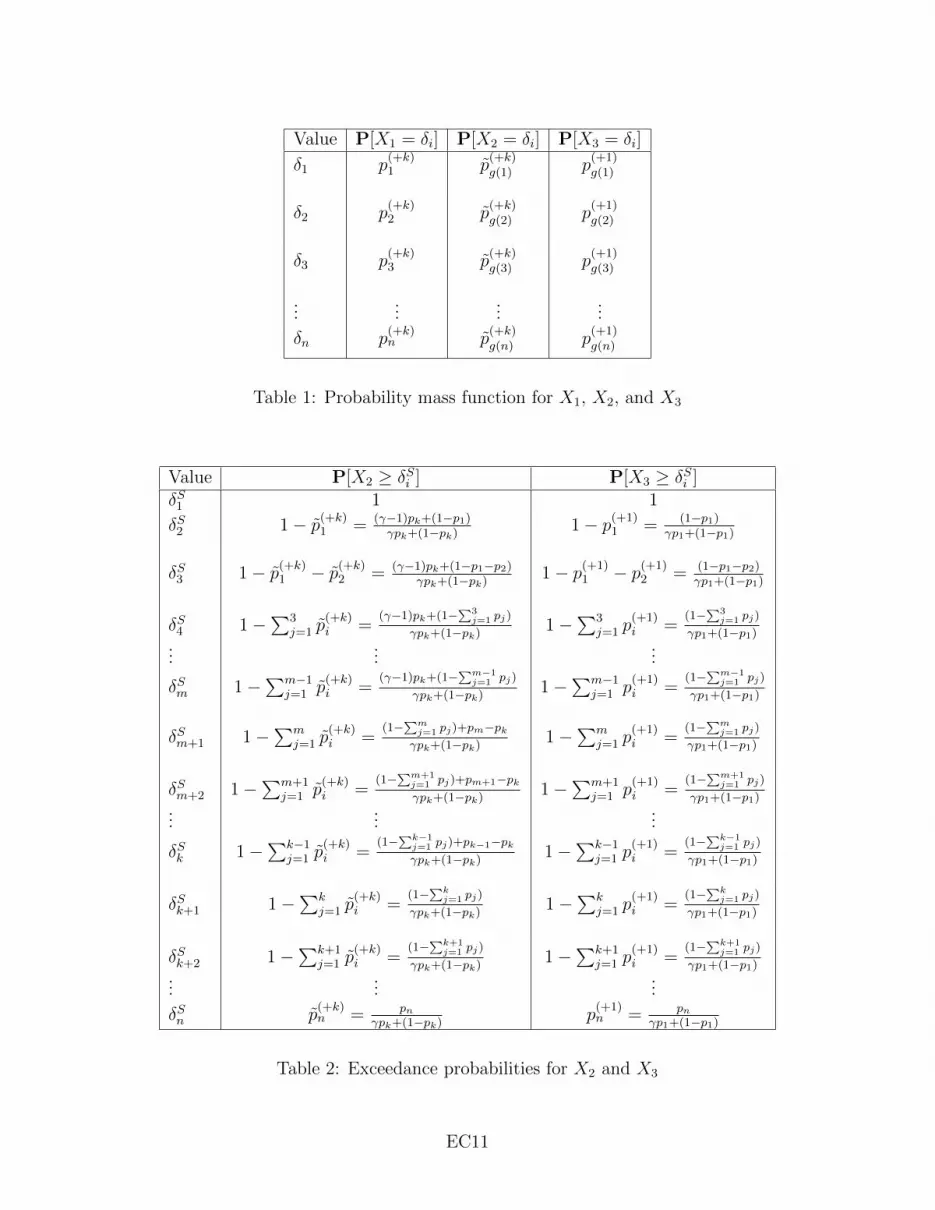
to each of those n values. The probability mass functions for X1, X2, and X3 appear in Table

1. For X1 we have P[X1 = δi] = p(+k)i and hence E[X1] = (p(+k))T δ.

To define X2 and X3 we first sort the elements of δ in ascending order and denote this

vector δS: δi corresponds to the ith element of δ, whereas δSi is the ith smallest element of

δ. Hence, min δ = δS1 ≤ δS2 ≤ . . . ≤ δSn = max δ. By defining an appropriate tie-breaking

rule for duplicate values in δ (e.g., by original ordering), there is a one-to-one correspondence

between the elements of δ and the elements of δS. With this correspondence, we can define the

invertible function g(·) that maps elements of δ to elements of δS. By construction, this leads

to the relationship δSg(i) = δi. The g function effectively ranks the values in δ in ascending

order. Before defining X2 we must also define a sorted version of p(+k). The vectors p and

p(+1) are sorted in decreasing order. However, p(+k) may not be sorted because in transitioning

from p to p(+k) the kth value increases while the other values decrease. The kth element of

p(+k) is the only value that is possibly out of order, so we only need to move that value to

the correct index and shift the remaining values to produce a sorted version of p(+k). Assume

that p(+k)k is now the mth largest value of p(+k) for some m ≤ k: p

(+k)m ≤ p

(+k)k < p

(+k)m−1. We

define p(+k) as the sorted version of p(+k) with p(+k)k moved to index m. The following lists

p, p(+1), p(+k), and p(+k)

p = ( p1, p2, p3, . . . , pm−1, pm, pm+1, . . . , pk−1, pk, pk+1, . . . , pn) (EC.23)

p(+1) =1

γp1 + (1− p1)(γp1, p2, p3, . . . , pm−1, pm, pm+1, . . . , pk−1, pk, pk+1, . . . , pn) (EC.24)

p(+k) =1

γpk + (1− pk)( p1, p2, p3, . . . , pm−1, pm, pm+1, . . . , pk−1, γpk, pk+1, . . . , pn) (EC.25)

p(+k) =1

γpk + (1− pk)( p1, p2, p3, . . . , pm−1, γpk, pm , . . . , pk−2, pk−1, pk+1, . . . , pn). (EC.26)

We define X2 by using p(+k): P[X2 = δi] = p(+k)g(i) . This assigns the largest probabilities in

EC9

p(+k) to the smallest values of δ. Thus E[X2] ≤ E[X1].

Finally we define X3 with the probability vector p(+1): P[X3 = δi] = p(+1)g(i) . Table 2

presents the exceedance probabilities P[X2 ≥ δSi ] and P[X3 ≥ δSi ]. Table 1 lists the values in

terms of δi, whereas Table 2 lists the values in terms of δSi so that the exceedance probabilities

will be non-increasing as we move down the table. By the construction of the ranking function

g(·), P[X3 = δSi ] = p(+1)i and therefore P[X3 ≥ δSi ] = 1−

∑i−1j=1 p

(+1)j . We write out the values

in Table 2 in terms of p using the expressions in (EC.24) and (EC.26). A comparison of the

columns in Table 2 reveals that X2 stochastically dominates X3. To see this note that the

denominators (numerators) in the X2 column are always less (greater) than the corresponding

denominators (numerators) in the X3. This stochastic dominance implies E[X3] ≤ E[X2] and

by transitivity E[X3] ≤ E[X1]. Furthermore there exists some j such that pji = p(+1)g(i) for all i,

so that the probability mass function of X3 corresponds to the jth column of P . This allows

us to write E[X3] = (pj)T δ and we have derived condition (EC.22)

(pj)T δ = E[X3] ≤ E[X1] = (p(+k))T δ.

Therefore any solution y∗ that produces an objective value less than 1 must be infeasible.

Specifically we have shown the jth constraint of (EC.19) is infeasible for index j defined

above. Since the dual has an optimal solution of 1, the primal defined in (EC.15)–(EC.17)

is feasible and the proof is complete.

EC10

Value P[X1 = δi] P[X2 = δi] P[X3 = δi]

δ1 p(+k)1 p

(+k)g(1) p

(+1)g(1)

δ2 p(+k)2 p

(+k)g(2) p

(+1)g(2)

δ3 p(+k)3 p

(+k)g(3) p

(+1)g(3)

......

......

δn p(+k)n p

(+k)g(n) p

(+1)g(n)

Table 1: Probability mass function for X1, X2, and X3

Value P[X2 ≥ δSi ] P[X3 ≥ δSi ]δS1 1 1

δS2 1− p(+k)1 = (γ−1)pk+(1−p1)γpk+(1−pk)

1− p(+1)1 = (1−p1)

γp1+(1−p1)

δS3 1− p(+k)1 − p(+k)2 = (γ−1)pk+(1−p1−p2)γpk+(1−pk)

1− p(+1)1 − p(+1)

2 = (1−p1−p2)γp1+(1−p1)

δS4 1−∑3

j=1 p(+k)i =

(γ−1)pk+(1−∑3j=1 pj)

γpk+(1−pk)1−

∑3j=1 p

(+1)i =

(1−∑3j=1 pj)

γp1+(1−p1)...

......

δSm 1−∑m−1

j=1 p(+k)i =

(γ−1)pk+(1−∑m−1j=1 pj)

γpk+(1−pk)1−

∑m−1j=1 p

(+1)i =

(1−∑m−1j=1 pj)

γp1+(1−p1)

δSm+1 1−∑m

j=1 p(+k)i =

(1−∑mj=1 pj)+pm−pkγpk+(1−pk)

1−∑m

j=1 p(+1)i =

(1−∑mj=1 pj)

γp1+(1−p1)

δSm+2 1−∑m+1

j=1 p(+k)i =

(1−∑m+1j=1 pj)+pm+1−pkγpk+(1−pk)

1−∑m+1

j=1 p(+1)i =

(1−∑m+1j=1 pj)

γp1+(1−p1)...

......

δSk 1−∑k−1

j=1 p(+k)i =

(1−∑k−1j=1 pj)+pk−1−pkγpk+(1−pk)

1−∑k−1

j=1 p(+1)i =

(1−∑k−1j=1 pj)

γp1+(1−p1)

δSk+1 1−∑k

j=1 p(+k)i =

(1−∑kj=1 pj)

γpk+(1−pk)1−

∑kj=1 p

(+1)i =

(1−∑kj=1 pj)

γp1+(1−p1)

δSk+2 1−∑k+1

j=1 p(+k)i =

(1−∑k+1j=1 pj)

γpk+(1−pk)1−

∑k+1j=1 p

(+1)i =

(1−∑k+1j=1 pj)

γp1+(1−p1)...

......

δSn p(+k)n = pn

γpk+(1−pk)p(+1)n = pn

γp1+(1−p1)

Table 2: Exceedance probabilities for X2 and X3

EC11

C Corollary 1: Threshold Policy for n = 2 Cells

The optimality of a threshold policy follows immediately from Proposition EC.2 in Appendix

B, which states the engage region is convex. The searcher should engage if p1 = 1 because

he achieves the minimum cost of 0 and the cost to wait is at least ρ1+ρ

α. A convex subset

of the interval [12, 1] that contains the point 1 must be a subinterval of the form [τ, 1]. This

completes the proof for Corollary 1.

The more interesting aspect is deriving an expression of τ as a function of the model

parameters q, α and ρ. As the expression, and accompanying derivation, of τ is quite com-

plicated we present it in the next section.

EC12

D Derivation of Optimal Two-cell Threshold τ

In this section we derive the threshold τ for the n = 2 case.

Proposition EC.4. The searcher should engage if and only if p1 ≥ τ for the following τ :

τ =

0.5 if 1

2≥ ρ

1+ρ(1− α) + 1

1+ρq

sup{p1 | 1− p1 = h(p1, q, α, ρ), p1 ∈ [0.5, 1]} otherwise,

where

h(p1, q, α, ρ) = α +GU

(1

1 + ρ, q, 1, B∗(p1)

)(−αp1 − (α− 1)(1− p1)

1

γ

)

+GL

(1

1 + ρ, q, 1, B∗(p1)

)(−α(1− p1)γB

∗(p1) − (α− 1)p1)

(EC.27)

B∗(p1) = −

2 log(

1−p1

p1

)log γ

(EC.28)

GU(x, q, A,B) =f1(x, q)

B − f2(x, q)B

f1(x, q)A+B − f2(x, q)A+B(EC.29)

GL(x, q, A,B) =

(1− qq

)Bf1(x, q)

A − f2(x, q)A

f1(x, q)A+B − f2(x, q)A+B(EC.30)

f1(x, q) =1 +

√1− 4q(1− q)x2

2qx(EC.31)

f2(x, q) =1−

√1− 4q(1− q)x2

2qx. (EC.32)

The functions GU(·), GL(·), f1(·), f2(·) in equations (EC.29)–(EC.32) all relate to calcu-

lations involving the gambler’s ruin problem. To derive τ we view the searcher’s stopping

problem as choosing parameters of a gambler’s ruin problem, and then we leverage off the

rich results from that area.

EC13

We prove Proposition EC.4 in two parts by considering the two cases separately. In

Appendix D.1 we present Lemma EC.2, which examines the case where τ = 0.5; in this

situation the searcher engages immediately for any state vector p. In Lemma EC.3, appearing

in Appendix D.2, we consider the general case where τ > 0.5.

D.1 τ = 0.5 case: always engage

Lemma EC.2. τ = 0.5 if and only if 12≥ ρ

1+ρ(1− α) + 1

1+ρq.

Proof. We complete the proof by considering the the uniform state vector p =(12, 12

)and

manipulating the cost equation in (11). In this special case, C(p(+1)) = C(p(+2)) by symmetry.

Therefore we can write the cost function in state p =(12, 12

)as:

C(p) = min

(1

2,

ρ

1 + ρα +

1

1 + ρC(p(+1))

).

Showing that the searcher should engage in the uniform case if and only if 12≥ ρ

1+ρ(1− α) +

11+ρ

q completes the proof.

First we argue that if 12< ρ

1+ρ(1−α) + 1

1+ρq, the searcher should wait and hence τ > 0.5.

To see this consider the myopic policy where the searcher either engages or receives one more

tip and then engages. In the uniform case p(+1)1 = γ

γ+1= q. Using the myopic policy, the

searcher should wait if

1

2>

ρ

1 + ρα +

1

1 + ρ(1− q). (EC.33)

Rearranging reveals the desired condition:

wait if1

2<

ρ

1 + ρ(1− α) +

1

1 + ρq. (EC.34)

If condition (EC.34) holds, then the myopic policy produces a lower cost than engaging. Since

we have found a wait strategy (myopic policy) that produces a lower cost than engaging, the

EC14

optimal policy will also wait. Thus, if condition EC.34 holds τ > 0.5.

Next we show that if 12≥ ρ

1+ρ(1−α)+ 1

1+ρq, the searcher should engage and hence τ = 0.5.

First assume the condition holds:

1

2≥ ρ

1 + ρ(1− α) +

1

1 + ρq. (EC.35)

By (EC.33) and (EC.34), condition (EC.35) is equivalent to

1

2≤ ρ

1 + ρα +

1

1 + ρ(1− q). (EC.36)

Condition (EC.36) states that engaging now produces a lower cost than obtaining one more

tip and then engaging. We now proceed to show that if condition (EC.36) (and hence

(EC.35)) holds the searcher should engage. We do this via contradiction. Assume (EC.36)

holds but the searcher should wait. Assume the searcher waits until he receives s1 tips for

cell 1 and s2 tips for cell 2. Define p = (p1, p2) as the new state after receiving these tips. In

this case we can write the p in terms of the tip-differential between s1 and s2

p1 =γs1

γs1 + γs2=

γs1−s2

γs1−s2 + 1p2 =

γs2

γs1 + γs2=

γs2−s1

γs2−s1 + 1.

If we define ∆ = |s1 − s2|, then the cost to engage in state p is 1γ∆+1

. We can now view our

threshold policy τ in terms of a threshold on the tip-differential ∆. By the optimality of a

threshold policy, if the searcher should wait in the uniform state, there exists some integer

M ≥ 1 such that the searcher should wait for ∆ ≤ M − 1 but engage when ∆ = M . Define

p(m) to be the state when the tip-differential in favor of cell 1 is m:

p1(m) =γm

γm + 1, p2(m) =

1

γm + 1.

By assumption we have that the searcher should wait in state p(M − 1) but engage in state

p(M). Consequently we have the following relationship (by definition of the cost function in

EC15

(11))

1

γM−1 + 1>

ρ

1 + ρα+

1

1 + ρ(r1(p(M − 1))

1

γM + 1+ (1− r1(p(M − 1)))C(p(M − 2))). (EC.37)

Because C(p) is a concave function that achieves a maximum at C(1/2) (see Proposition

EC.1) and C(1) = 0, C(p) decreases over the interval p ∈ [1/2, 1]. Hence C(p(M − 2)) ≥

C(p(M)) = 1γM+1

. Substituting this relationship into (EC.37) produces

1

γM−1 + 1>

ρ

1 + ρα +

1

1 + ρ

1

γM + 1. (EC.38)

We now proceed to show that conditions (EC.36) and (EC.38) are incompatible. Let us

rewrite these conditions to highlight their connection

1

2− 1

1 + ρ(1− q) ≤ ρ

1 + ρα (EC.39)

1

γM−1 + 1− 1

1 + ρ

1

γM + 1>

ρ

1 + ρα, (EC.40)

where (EC.39) corresponds to (EC.36) and (EC.40) corresponds to (EC.38). Condition

(EC.39) is an assumption and condition (EC.40) follows because we assume that the searcher

waits in the uniform state and engages when ∆ = M ≥ 1. The left-hand sides of (EC.39)

and (EC.40) have the form g(i), where

g(i) =1

γi−1 + 1− 1

1 + ρ

1

γi + 1.

The left-hand side of (EC.39) corresponds to g(1) and (EC.40) corresponds to g(M). Because

we assume that the myopic policy of receiving one tip and engaging (i.e., M = 1) produces a

higher cost than engaging immediately (condition (EC.36)), we must have M > 1. Inspection

EC16

of g(i) reveals it is a strictly decreasing function. Consequently

g(M) < g(1)

1

γM−1 + 1− 1

1 + ρ

1

γM + 1<

1

2− 1

1 + ρ(1− q),

which implies an incompatibility between conditions (EC.39) (equivalently (EC.35) or (EC.36))

and (EC.40) (equivalently (EC.38)). Therefore if condition (EC.35) holds the searcher must

engage, and τ = 0.5.

D.2 τ > 0.5 case

In this section we consider the general case of Proposition EC.4. The proof is involved

with many lemmas to break it into more manageable pieces. It relies on analyzing the tip-

differential between cell 1 and cell 2 as a random walk. A threshold policy on p1 can be

viewed as defining absorbing boundaries on this random walk. We then leverage gambler’s

ruin machinery to derive the quantities of interest. Lemma EC.3 states the desired result.

Lemma EC.3. If 12< ρ

1+ρ(1− α) + 1

1+ρq, the optimal threshold is given by

τ = sup{p1 | 1− p1 = h(p1, q, α, ρ), p1 ∈ [0.5, 1]},

where equation (EC.27) defines h(·).

Proof. To start we consider a general threshold policy given by parameter T ∈ (1/2, 1). The

searcher should wait until the first time that p1 ≥ T and then the searcher engages. We use

T to denote an arbitrary threshold policy and τ to denote the optimal threshold policy. In

Lemma EC.4 we show that for a given p1, the cost associated with using threshold policy T

EC17

is given by

g(T, p1, q, α, ρ) =

1− p1 if T ≤ p1

α+GU

(1

1+ρ , q, AT , BT

)(−αp1 − (α− 1)(1− p1) 1

γAT

)+GL

(1

1+ρ , q, AT , BT

) (−α(1− p1)γBT − (α− 1)p1

)if T > p1,

(EC.41)

where GU(·) is defined in (EC.29), GL(·) is defined in (EC.30), and

AT =

⌈log T (1−p1)

(1−T )p1

log γ

⌉(EC.42)

BT = −

⌊log (1−T )(1−p1)

Tp1

log γ

⌋. (EC.43)

AT is the minimum tip-differential in favor of cell 1 required for the updated posterior

probability of cell 1 to exceed the threshold T . BT is the minimum differential in favor of

cell 2 required for the updated posterior probability of cell 2 to exceed the threshold T .

BT ≥ AT because p1 ≥ 1/2. For a given p1 we can find an optimal threshold by solving

minT g(T, p1, q, α, ρ). For any particular p1 the optimal threshold is not unique because of

the discrete nature of tips. A range of T (depending upon the p1 of interest) around the true

optimal threshold τ will produce optimal results.

Next comparing (EC.27) and (EC.41) we see that

h(p1, q, α, ρ) = limT↓p1

g(T, p1, q, α, ρ).

That is we can view h(p1, q, α, ρ) as the expected cost when we use a threshold infinitesimally

greater than p1. Using this policy the searcher will engage with a tip-differential of one in

favor of cell 1 or a tip-differential of B∗(p1) (see equation (EC.28)) in favor of cell 2. Recall

that B∗(p1) is the minimum tip-differential in favor of cell 2 such that the updated posterior

probability for cell 2 exceeds p1. Using the parameter ∆ defined in Lemma EC.4 as the

tip-differential in favor of cell 1, then h(p1, q, α, ρ) is the expected cost from using the policy

EC18

“wait until ∆ = 1 or ∆ = −B∗(p1)”. The way to think about the result for this proposition

is to compare the cost to engage (1− p1) to the cost of using the policy “wait until ∆ = 1 or

∆ = −B∗(p1)” (h(p1, q, α, ρ)).

To complete the proof, we first show in Lemma EC.5 that the optimal threshold τ satisfies

τ = sup{p1 | 1− p1 > h(p1, q, α, ρ), p1 ∈ [0.5, 1]}. (EC.44)

In Lemma EC.6 we show that this τ satisfies (1 − τ) = h(τ, q, α, ρ), and finally in Lemma

EC.7 we show that

1− p1 < h(p1, q, α, ρ) ∀τ < p1 ≤ 1.

Combining the pieces from Lemmas EC.5–EC.7 produces the desired result:

τ = sup{p1 | 1− p1 = h(p1, q, α, ρ), p1 ∈ [0.5, 1]}.

Note the expression for h(p1, q, α, ρ) simplifies significantly for B∗(p1) = 1. As we ap-

proach p1 = 1/2, B∗(p1) eventually equals 1 for any values of q, α, ρ. When B∗(p1) = 1, the

searcher uses the myopic policy: engage after the first tip. The cost in this case simplifies to:

limp1↓1/2

h(p1, q, α, ρ) =

(1−

(ρ

1 + ρ(1− α) +

1

1 + ρq

)). (EC.45)

Condition (EC.45) is similar to the condition for whether τ = 0.5 (e.g., see condition (EC.34)).

This leads to the relationship

limp1↓1/2

h(p1, q, α, ρ) <1

2⇐⇒ τ > 0.5.

Thus the conditions for the τ > 0.5 case and the τ = 0.5 are consistent.

EC19

Lemma EC.4. For a given p1, the expected cost associated with using threshold policy T is

given by the function g(T, p1, q, α, ρ) defined by equation (EC.41).

Proof. Recall that we can update the state probability vector p after receiving M tips if we

know the number of tips for cell 1 (s1) and the number of tips for cell 2 (s2 = M − s1). The

updated probabilities only depend upon the tip-differential s1− s2 (see equations (13)–(14)).

If we define ∆ = s1 − s2, then we can transform the threshold policy from “engage as soon

as p1 ≥ T” to a threshold policy on ∆: engage as soon as ∆ ≥ AT or ∆ ≤ −BT . The specific

formulas for AT and BT appear in equations (EC.42)–(EC.43); both BT and AT depend upon

the threshold T and the initial state vector p. If T ≤ p1 then AT ≤ 0 and the searcher should

engage immediately. If T > p1 then AT > 0 and the searcher should wait. Because both

p1 ≥ 1/2 and T > 1/2, we have that BT > 0. For the remainder of this Lemma, we will

assume that AT > 0 so that the searcher does not trivially engage immediately.

Given an initial state vector p and threshold T , we compute AT and BT from equations

(EC.42)–(EC.43). The searcher will continue receiving tips until one of three events occur:

the target attacks, the tip-differential reaches ∆ = AT (searcher engages cell 1), the tip-

differential reaches ∆ = −BT (searcher engages cell 2). To compute the expected cost of

using the threshold policy T , we need to determine the probabilities of each of these three

events occurring and their associated costs.

If we condition on the location of the target, then ∆ proceeds according to a random

walk. If cell 1 (cell 2) contains the target, then ∆ increases by 1 at each step with probability

q (1−q) and decreases by 1 with probability 1−q (q). We utilize random walk and gambler’s

ruin results to examine when the searcher will engage and whether the searcher engages when

∆ = AT or ∆ = −BT . For the given threshold T , we can define a stopping time NT when

the searcher engages. Define ∆i to be the value of the tip-differential ∆ after the ith tip, so

∆0 = 0. We then define the stopping time NT as

NT = inf{i | ∆i ∈ {−BT , AT}}.

EC20

If we further define Yn as the cost incurred after receiving n tips, then the random cost

incurred from using the stopping rule NT is given by

YNT =αI(attack occurs before tip NT )

+ I(attack occurs after tip NT )I(engage wrong cell).

We now compute our desired quantity: the expected cost from using threshold policy T

E[YNT ] =αP[attack occurs before tip NT ]

+ P[attack occurs after tip NT and choose wrong cell]. (EC.46)

The false positive cost in (EC.46) depends on the actual cell location of the target and

whether the ∆ random walk stops at −BT or AT :

P[attack occurs after tip NT and choose wrong cell]

= p1P[attack occurs after tip NT , ∆NT = −BT | target in cell 1]

+ (1− p1)P[attack occurs after tip NT , ∆NT = AT | target in cell 2]. (EC.47)

Focusing on the first term in (EC.47), we condition on the value of NT :

P[attack occurs after tip NT , ∆NT = −BT | target in cell 1]

=∞∑i=0

(1

1 + ρ

)iP[NT = i,∆NT = −BT | target in cell 1]. (EC.48)

Fortunately, explicit expressions exist for the generating function term in (EC.48). Boccio

(2012) presents several gambler’s ruin results, including the generating functions relevant to

our problem. Utilizing equation (45) of Boccio (2012) we can write

EC21

P[attack occurs after tip NT , ∆NT= −BT | target in cell 1] = GL

(1

1 + ρ, q, AT , BT

)(EC.49)

P[attack occurs after tip NT , ∆NT= −BT | target in cell 2] = GL

(1

1 + ρ, 1− q, AT , BT

), (EC.50)

where GL(·) is defined in (EC.30). Furthermore, we can use equation (46) of Boccio

(2012) to express

P[attack occurs after tip NT , ∆NT= AT | target in cell 1] = GU

(1

1 + ρ, q, AT , BT

)(EC.51)

P[attack occurs after tip NT , ∆NT= AT | target in cell 2] = GU

(1

1 + ρ, 1− q, AT , BT

), (EC.52)

whereGU(·) is defined in (EC.29). By combining equations (EC.49) (equivalently (EC.50))

and (EC.51) (equivalently (EC.52)) we produce the probability the attack occurs after en-

gaging, conditioned on the location of the cell:

P[attack occurs after tip NT | target in cell 1] =GL

(1

1 + ρ, q, AT , BT

)+GU

(1

1 + ρ, q, AT , BT

)(EC.53)

P[attack occurs after tip NT | target in cell 2] =GL

(1

1 + ρ, 1− q, AT , BT

).

+GU

(1

1 + ρ, 1− q, AT , BT

)(EC.54)

Substituting equations (EC.47), (EC.48), (EC.49), (EC.52), (EC.53), and (EC.54) into (EC.46)

EC22

produces the complete expression

E[YNT ] =

p1

α

1−

GU(

1

1 + ρ, q, AT , BT

)︸ ︷︷ ︸prob reach AT before attack.

(choose cell 1 correctly)

+GL

(1

1 + ρ, q, AT , BT

)︸ ︷︷ ︸prob reach BT before attack.(choose cell 2 incorrectly)

︸ ︷︷ ︸

prob engage before attack

+GL

(1

1 + ρ, q, AT , BT

)︸ ︷︷ ︸prob reach BT before attack.(choose cell 2 incorrectly)

+ (1− p1)

α

1−

GU(

1

1 + ρ, 1− q, AT , BT

)︸ ︷︷ ︸

prob reach AT before attack.(choose cell 1 incorrectly)

+GL

(1

1 + ρ, 1− q, AT , BT

)︸ ︷︷ ︸

prob reach BT before attack.(choose cell 2 correctly)

︸ ︷︷ ︸

prob engage before attack

+GU

(1

1 + ρ, 1− q, AT , BT

)︸ ︷︷ ︸

prob reach AT before attack.(choose cell 1 incorrectly)

. (EC.55)

The first line of (EC.55) conditions on the target being in cell 1 and the second and third

lines condition on the target being in cell 2. Examination of equations (EC.29)–(EC.32)

reveals the following relationships

GU(x, q, A,B) = γAGU(x, 1− q, A,B) (EC.56)

GL(x, q, A,B) =1

γBGL(x, 1− q, A,B). (EC.57)

EC23

Using (EC.56) and (EC.57) we simplify (EC.55) to our final expression

E[YNT ] =

1− p1 if T ≤ p1 engage immediately

α +GU

(1

1+ρ, q, AT , BT

)(−αp1 − (α− 1)(1− p1) 1

γAT

)+GL

(1

1+ρ, q, AT , BT

) (−α(1− p1)γBT − (α− 1)p1

)if T > p1.

(EC.58)

Denoting g(T, p1, q, α, ρ) ≡ E[YNT ] completes the proof.

Lemma EC.5. The optimal threshold τ is defined by

τ = sup{p1 | 1− p1 > h(p1, q, α, ρ), p1 ∈ [0.5, 1]}.

Proof. Consider the set

D = {x | 1− x > h(x, q, α, ρ), x ∈ [0.5, 1]}.

If p1 ∈ D, then it is optimal to wait because we found a wait-policy that that performs better

than engaging. Namely the policy that waits until ∆ = 1 or ∆ = −B∗(p1) achieves a lower

cost (h(p1, q, α, ρ)) than engaging (1− p1).

We next define

τ = supD

and argue that τ ≤ τ . If τ ∈ D, then as argued above it is optimal to wait for p1 = τ .

Since the optimal policy is a threshold policy it must follow that τ > τ . If τ 6∈ D, then by

definition of the supremum, τ must be a limit point of D. In this case, if τ > τ , then there

would exist some p ∈ (τ, τ) and p ∈ D because τ is a limit point of D. This implies it is

EC24

optimal to wait for p1 = p ∈ D, but p is greater than the engage threshold τ by construction.

This is a contradiction. Hence τ ≤ τ

We next argue τ ≥ τ . We proceed by contradiction and assume τ < τ . We will find a

p ∈ (τ , τ) such that the policy “wait until ∆ = 1 or ∆ = −B∗(p)” is the optimal policy. Since

h(p, q, α, ρ) is the cost associated with this policy, then h(p, q, α, ρ) < (1− p). That is if it is

optimal to wait, then the optimal cost to wait must be strictly less than the cost to engage.

If that is the case then p ∈ D. However, p > τ = supD, which leads to a contradiction.

Thus τ ≥ τ . It remains to find such a p.

Any p such that p ∈ (L, τ) where L = max(τ , L1, L2, L3) and

L1 =τ

γ(1− τ) + τ, (EC.59)

L2 =1

1 + exp(− (B∗(τ)−1) log γ

2

) , (EC.60)

L3 =γB∗(τ)−1(1− τ)

γB∗(τ)−1(1− τ) + τ, (EC.61)

will suffice. By construction all are less than τ . L1 < τ by inspection because γ > 1. L1

ensures that one additional tip for cell 1 will push the updated maximum posterior probability

above the optimal threshold τ , where it is optimal to engage. L2 is constructed such that

B∗(L2) = B∗(τ)−1. This condition, coupled with inspection of (EC.28), reveals that L2 < τ .

We require L2 < p because this ensures that B∗(p) = B∗(τ). Finally by definition, B∗(τ) (see

(EC.28)) is the minimum tip-differential in favor of cell 2 such that the updated posterior

probability for cell 2 exceeds τ . Therefore,

L3 =γB∗(τ)−1(1− τ)

γB∗(τ)−1(1− τ) + τ< τ ≤ γB

∗(τ)(1− τ)

γB∗(τ)(1− τ) + τ. (EC.62)

Combining L2, L3 < p we see that a tip-differential of B∗(τ)− 1 = B∗(p)− 1 in favor of cell

EC25

2 is not enough to push the posterior for cell 2 above τ starting from p:

γB∗(τ)−1(1− p)

γB∗(τ)−1(1− p) + p=

γB∗(p)−1(1− p)

γB∗(p)−1(1− p) + pby L2 < p (EC.63)

< τ by L3 < p. (EC.64)

However, because p < τ and B∗(p) = B∗(τ) (by L2 < p) a tip-differential of B∗(p) = B∗(τ)

in favor of cell 2 does push the posterior for cell 2 above τ :

τ <γB∗(p)(1− p)

γB∗(p)(1− p) + p. (EC.65)

Combining conditions (EC.64) and (EC.65) produces

γB∗(p)−1(1− p)

γB∗(p)−1(1− p) + p< τ <

γB∗(p)(1− p)

γB∗(p)(1− p) + p. (EC.66)

Condition (EC.66) states that, starting from p1 = p, the updated posterior first exceeds the

optimal threshold τ with a tip-differential in favor of cell 2 when ∆ = −B∗(p). Thus for

∆ ∈ [−B∗(p) + 1, 0] the maximum posterior probability is below the optimal threshold τ

and the searcher should wait. The searcher should engage when ∆ first hits either ∆ = 1

or ∆ = −B∗(p). Engaging for ∆ ∈ {−B∗(p), 1} produces a maximum posterior probability

in excess of τ . We have completed the proof because we have found a p ∈ (τ , τ) where it

is optimal to wait and has optimal cost of h(p, q, α, ρ), which must be less than the cost to

engage (1− p). Therefore, we have produced a contradiction and so τ ≥ τ .

We have shown that τ ≤ τ and τ ≥ τ and thus our proof is complete:

τ = τ = supD = sup{p1 | 1− p1 > h(p1, q, α, ρ), p1 ∈ [0.5, 1]}.

Lemma EC.6. The optimal τ defined by equation (EC.44) satisfies (1− τ) = h(τ, q, α, ρ).

EC26

Proof. In Lemma EC.5 we showed that the optimal threshold τ is defined by

τ = sup{p1 | 1− p1 > h(p1, q, α, ρ), p1 ∈ [0.5, 1]}.

Now we show that the threshold satisfies (1− τ) = h(τ, q, α, ρ). The quantity h(τ, q, α, ρ) is

the cost associated with the policy “wait until ∆ = 1 or ∆ = −B∗(τ)”. By definition it is

optimal for the searcher to engage at p1 = τ . However, if the searcher chose to wait in an

optimal fashion, then he would use the policy associated with h(τ, q, α, ρ): wait until ∆ = 1

or ∆ = −B∗(τ). Thus h(τ, q, α, ρ) is the optimal cost to wait with p1 = τ (corresponding to

the second term of (11)). At the threshold, the cost to engage must equal the optimal cost

from waiting. This follows from the concavity of the cost function C(p). If the cost to engage

did not equal the optimal cost from waiting at the threshold, this would imply a discontinuity

in the cost function (impossible by concavity) or that the threshold is incorrect. Therefore

(1 − τ) = h(τ, q, α, ρ). To see this more rigorously consider the values L1, L2, L3 from

(EC.59)–(EC.61). As discussed in the proof for Lemma EC.5, for p1 ∈ (max(L1, L2, L3), τ)

the optimal cost is given by h(p1, q, α, ρ). However, because B∗(p1) = B∗(τ) in this range of

interest, h(p1, q, α, ρ) is just a linear function of p1. Thus, we can write out the cost function

C(p) explicitly for p1 > max(L1, L2, L3) in terms of a piecewise linear function

C(p) =

α +GU

(1

1+ρ, q, 1, B∗(τ)

)(−αp1 − (α− 1)(1− p1) 1

γ

)+GL

(1

1+ρ, q, 1, B∗(τ)

) (−α(1− p1)γB

∗(τ) − (α− 1)p1)

if max(L1, L2, L3) < p1 < τ

1− p1 if p1 ≥ τ.

We know C(p) is concave and thus the two linear pieces must intersect at the threshold τ .

This completes the proof: (1− τ) = h(τ, q, α, ρ).

EC27

Lemma EC.7. For the optimal τ defined by equation (EC.44) we have the following condition

1− p1 < h(p1, q, α, ρ), ∀τ < p1 ≤ 1.

Proof. h(p1, q, α, ρ) is the cost associated with the policy “wait until ∆ = 1 or ∆ = −B∗(p1)”.

This cost must be greater than the optimal cost to wait from our cost function C(p) (from

(11))

h(p1, q, α, ρ) ≥ ρ

1 + ρα +

1

1 + ρ

2∑i=1

ri(p)C(p(+i)).

Thus to complete the proof it suffices to show that

1− p1 <ρ

1 + ρα +

1

1 + ρ

2∑i=1

ri(p)C(p(+i)), ∀τ < p1 ≤ 1. (EC.67)

For the region of interest it is always optimal to engage in state p(+1). Thus C(p(+1)) =

(1 − p(+1)1 ). The optimal policy for state p(+2) depends upon how close p1 is to τ . Let us

denote K(p) as the optimal cost to wait and rewrite it

K(p) =ρ

1 + ρα +

1

1 + ρ

2∑i=1

ri(p)C(p(+i))

=ρ

1 + ρα +

1

1 + ρ

(r1(p)(1− p(+1)

1 ) + r2(p)(1− p(+2)1 )

)− 1

1 + ρr2(p)

((1− p(+2)

1 )− C(p(+2))). (EC.68)

It is a straightforward exercise to show that

r1(p)(1− p(+1)1 ) + r2(p)(1− p(+2)

1 ) = 1− p1. (EC.69)

EC28

Substituting (EC.69) into (EC.68) yields

K(p) =ρ

1 + ρα +

1

1 + ρ(1− p1)−

1

1 + ρr2(p)

((1− p(+2)

1 )− C(p(+2))).

Condition (EC.67) is equivalent to (1−p1) < K(p). Because τ is the optimal engage threshold,

it must hold that (1− p1) ≤ K(p) over the region of interest. Thus to complete the proof we

need to show that (1−p1) 6= K(p) for p1 > τ . We show this condition holds by contradiction.

Let us assume that condition (EC.67) does not hold. Therefore there exists some state p =

(p1, (1−p1)), such that p1 > τ and the cost to engage equals the cost to wait: (1−p1) = K(p).

We will show this implies that for the state p = (p1−ε, (1−p1+ε)), such that p1 = p1−ε > τ ,

we have the relationship (1− p1) > K(p). This implies it is optimal to wait in state p, which

is a contradiction because p1 exceeds the engage threshold: p1 = p1 − ε > τ . Let us examine

K(p)

K(p) =ρ

1 + ρα+

1

1 + ρ(1− p1)− 1

1 + ρr2(p)

((1− p(+2)

1 )− C(p(+2)))

=ρ

1 + ρα+

1

1 + ρ(1− p1)− 1

1 + ρr2(p)

((1− p(+2)

1 )− C(p(+2)))

+1

1 + ρε

=ρ

1 + ρα+

1

1 + ρ(1− p1)− 1

1 + ρr2(p)

((1− p(+2)

1 )− C(p(+2)))

+1

1 + ρ

(ε−

[r2(p)

((1− p(+2)

1 )− C(p(+2)))− r2(p)

((1− p(+2)

1 )− C(p(+2)))])

=K(p)

+1

1 + ρ

(ε−

[r2(p)

((1− p(+2)

1 )− C(p(+2)))− r2(p)

((1− p(+2)

1 )− C(p(+2)))])

. (EC.70)

The final key is showing the term is square brackets is non-negative. To do this first note

that

r2(p) > r2(p) (EC.71)

because p1 < p1. This follows from the definition of ri(·) in equation (7) and q > 1/2. Next

EC29

for any state p,

1− p1 ≥ C(p) (EC.72)

because C(p) is the optimal cost and (1− p1) is greater than or equal to the cost to engage

(it only equals the cost to engage if p1 ≥ 1/2). Furthermore, we have

1− p1 = C(p) for p ≥ τ, (EC.73)

since it is optimal to engage for p ≥ τ . Finally by concavity

C(p) is concave as we increase p1. (EC.74)

Combining conditions (EC.72)–(EC.74) produces the following condition:

(1− p1)− C(p) is non-increasing as we increase p1 over [0, 1]. (EC.75)

Because p1 < p1 (and hence p(+2)1 < p

(+2)1 ) we can combine conditions (EC.71) and (EC.75)

to produce the desired result

r2(p)(

(1− p(+2)1 )− C(p(+2))

)− r2(p)

((1− p(+2)

1 )− C(p(+2)))≥ 0. (EC.76)

Substituting (EC.76) into (EC.70 ) yields

K(p) ≤K(p) +1

1 + ρε.

By assumption K(p) = (1−p1) and thus we have shown the desired contradictory condition:

K(p) ≤(1− p1) +1

1 + ρε < (1− p1 + ε) = (1− p1).

EC30

Consequently, condition (EC.67) must hold and the proof is complete:

1− p1 < h(p1, q, α, ρ), ∀τ < p1 ≤ 1.

E Expected Number of Tips

The search ends either when the searcher engages or the target attacks. In this section

we compute the expected number of tips received during the search, accounting for both

possible ending scenarios. For a given set of parameters α, ρ and q we first compute τ from

Proposition EC.4. Starting from the uniform state p = (0.5, 0.5), we next examine when the

tip-differential ∆ will cause the posterior probability to exceed the threshold τ . Inspection

of equation (13) reveals that the searcher will engage when the tip-differential ∆ first reaches

Aτ (and the searcher engages cell 1) or −Aτ (and the searcher engages cell 2), where

Aτ =

⌈log τ

1−τ

log γ

⌉. (EC.77)

We model ∆i as the tip-differential after the ith tip with ∆0 = 0. If we condition on cell 1

containing the target, then ∆i follows a random walk that increases by 1 with probability q

and decreases by 1 with probability (1−q). We define a Markov chain for ∆i that incorporates

the potential for the mature attack by the target. ∆i proceeds as a random walk on the state

space {−Aτ ,−(Aτ−1), . . . ,−1, 0, 1, . . . , Aτ−1, Aτ}, and we add a state X to denote the target

attacking before the next tip. The Markov chain has three absorbing states: {−Aτ , Aτ ,X}

EC31

and when ∆i is in a non-absorbing state it transitions according to the following dynamics

∆i+1 =

∆i + 1 with probability q 1

1+ρ

∆i − 1 with probability (1− q) 11+ρ

X with probability ρ1+ρ

.

(EC.78)

The search ends when the Markov chain transitions to one of the absorbing states. We can

now define a system of equations to solve for the expected number of tips the searcher receives

before the search ends. Denote Tj as the expected number of tips until the search ends when

the system starts with ∆0 = j. We present T0 in Figure 2. If τ = 0.5 then T0 = 0 because

the searcher engages immediately. Otherwise the Ti satisfy the following system of equations

Ti = 1 + q1

1 + ρTi−1 + (1− q) 1

1 + ρTi−1 −

ρ

1 + ρ, for − Aτ < i < Aτ (EC.79)

TAτ = T−Aτ = 0. (EC.80)

Solving the system of equations given by (EC.79)–(EC.80) is a straighforward linear algebra

exercise. Note we subtract ρ1+ρ

in equation (EC.79) because the searcher does not receive a

tip if the target attacks. We can condition on cell 2 containing the target and compute a

similar expected number of tips and then combine the two quantities to calculate the final

unconditional expected number of tips. Not surprisingly the conditional expected number of

tips is the same for the two locations.

F n =∞

In Appendix F.1 we provide the mathematical motivation for the problem. We prove Propo-

sition 2 in Appendix F.2. Finally in Appendix F.3 we compute the costs for the finite n

heuristic and evaluate its performance.

EC32

F.1 Motivation

Assume we have n cells and consider a maximum of m < n tips provided to the searcher. We

will show in this section that for large enough m and n, the searcher will receive a second tip

for some cell by tip m with high probability, and the searcher will engage that cell once he

receives the repeat tip.

First we compute the probability that the informant provides no repeat tips in the first m

tips. Define Xm as the number of tips pointing to cell 1, which is a binomial random variable

with parameters m and q. The probability of no repeats in any cell in the first m tips is less

than the probability of no repeats to cell 1 in the first m tips. Therefore

P[no repeats in m tips] ≤ P [Xm ≤ 1] = (1− q)m +mq(1− q)m−1 ≤ 2m(1− q)m−1 → 0 (EC.81)

Thus for any ε > 0, we can use condition (EC.81) to find an m0 such that for any m0 < m < n

we have P[no repeats in m tips] < ε.

Next we will show that for large enough n relative to our choice of m > m0, the searcher

will engage if some cell receives its second tip prior to tip m. Assume that tip m is the first

time a cell receives a second tip. Thus the first m − 1 tips point to distinct cell. Since we

assume a uniform prior, the posterior of cell 1, which receives the second tip, is

p1 =γ2

γ2 + (m− 2)γ + (n−m+ 1)=

(q

1−q

)2(n− 1)(

q1−q

)2(n− 1) + (m− 2) q

1−q + n−m+1n−1

(EC.82)

This follows directly from equation (4). Clearly, the expression for p1 in (EC.81) converges to

1 as n→∞ for fixed q and m. Consequently for some n > n0, p1 will exceed the condition to

engage in (15) and the searcher will engage no later than the first time he receives a repeat

tip as long as the first repeat tip occurs before m. Note of course, it may be optimal to

engage before that.

Putting the pieces together, we have for any m > m0 that there is less than probability

EC33

ε that we will receive more than m tips before our first repeat. We can then use equation

(EC.82) to show that if and when that repeat occurs, the searcher will engage if n > n0,m.

This motivates the infinite cell case: for large n with high probability the searcher will

engage no later than when he receives the first repeat tip.

F.2 Proof of Proposition 2

We re-list the three possible optimal alternatives for convenience

1. Engage any cell: cost 1

2. Obtain one tip and engage the corresponding cell: cost ρ1+ρ

α + 11+ρ

(1− q)

3. Engage the first cell to receive two tips: cost α

(1−

(qρ+q

)2).

To complete the proof we must complete three tasks: (1) derive the costs provided for

each option, (2) show that any other option is suboptimal, (3) show the minimal cost option

corresponds to the conditions in Proposition 2. We perform task 1 in Appendix F.2.1, task

2 in Appendix F.2.2, and task 3 in Appendix F.2.3.

F.2.1 Cost Associated with Three Options

If the searcher engages immediately (option 1), he will not detect the correct cell and thus

collateral damage is guaranteed, yielding a cost of 1.

If the searcher chooses option 2, then with probability ρ1+ρ

the target attacks, which

generates a cost of α. With probability 11+ρ

the searcher receives the tip. The informant

points to the correct cell with probability q. Thus if the the searcher engages after this tip,

he will choose incorrectly with probability (1−q), causing collateral damage. This completes

the derivation of the cost for option 2. Another way to compute this cost is to start with

finite n and uniform prior. After one tip, the state transitions from p = (1/n, 1/n, . . . , 1/n)

to p+1 = (q, (1−q)/(n−1), . . . , (1−q)/(n−1)). See equation (5) for the transition dynamics.

Since p+11 = q for any n, this will also hold in the limit as n→∞.

EC34

The derivation for option 3 is slightly more complicated. If the searcher waits until he

receives a confirming tip, then he know with certainty that cell contains the target. The

only cost that can occur for option 3 is if the target attacks before the searcher receives the

confirming tip. Therefore, we proceed to compute the probability the searcher will receive

the confirming tip before the target attacks.

We first compute the probability the searcher will receive the confirming tip on tip m ≥ 2.

For this to occur, the mth tip points to cell 1 (prob q), and in the first m − 1 tips, m − 2

tips point to a wrong cell (probability (1 − q)m−2) and one points to cell 1 (probability q).

Since the first tip pointing to cell 1 can occur in any of the first m− 1 tips, the probability

that the confirming tip occurs on the mth tip is (m − 1)q(1 − q)m−2q. Finally, the target’s

attack must not occur before the mth tip, which happens with probability 1/(1 + ρ)m. We

now sum over all possible values of m for the final probability:

P[confirming tip before attack] =∞∑i=2

(i− 1)q(1− q)i−2q(

1

1 + ρ

)i=

q2

1− q

(1

1 + ρ

) ∞∑i=2

(i− 1)(1− q)i−1(

1

1 + ρ

)i−1=

q2

1− q

(1

1 + ρ

) ∞∑i=2

(i− 1)

((1− q) 1

1 + ρ

)i−1=

q2

1− q

(1

1 + ρ

) ∞∑i=1

i

((1− q) 1

1 + ρ

)i.

Using geometric series results this simplifies to

P[confirming tip before attack] =q2

1− q1

1 + ρ

(1− q) 11+ρ(

1− (1− q) 11+ρ

)2=

(q

ρ+ q

)2

.

EC35

Thus the expected cost for choosing option 3 is the desired result:

E[cost of option 3] = αP[attack occurs before confirming tip]

= α(1−P[confirming tip before attack])

= α

(1−

(q

ρ+ q

)2).

F.2.2 Suboptimality of Other Options

The searcher will engage after receiving a confirming tip because that state generates 0 cost.

Thus to determine the optimal policy we only need to consider the searcher engaging on or

before the confirming tip. Proposition 2 lists two additional options: engage before receiving

any tips or engage the cell pointed to by the first tip. We need to consider one final option:

engage after the first tip but before the confirming tip. In this section we show this option

is suboptimal and thus we only need to consider the three options listed in Proposition 2.

Let us define a related stopping problem where the searcher has received m tips about

m different cells. The searcher has the option of waiting or engaging one of the m cells

uniformly. We will use m as our state variable. Before defining the cost function we will

derive some important probabilities. The searcher reaches state m (ignoring the possibility

of attack) with probability (1 − q)m + mq(1 − q)m−1, which accounts for either m incorrect

tips or 1 correct tip and m− 1 incorrect tips. This implies

P[first m tips contain correct cell] =mq

(1− q) +mq, (EC.83)

which converges to 1 as m increases. If the searcher engages he will choose an incorrect cell

if either (1) none of the m tips point to the correct cell, or (2) one of the m tips points to

the correct cell, but the searcher does not engage that cell. The first situation occurs with

EC36

probability

P[first m tips do not point to correct cell] =1− q

(1− q) +mq(EC.84)

The probability the second situation occurs, given the first m tips contain the correct cell, is

(m− 1)/m. Putting everything together we have

P[searcher chooses incorrect cell] =(1− q) + (m− 1)q

(1− q) +mq= 1− q

(1− q) +mq, (EC.85)

which monotonically approaches 1 as we increase m. Equation (EC.85) also represents the

cost for the searcher to engage in state m as we normalize collateral damage to 1. If the

searcher waits, then with the probability in (EC.84) the m tips do not contain the correct

cell and thus the system will transition to state m+1 (provided an attack does not occur). If

one of the m tips does contain the correct cell (probability in (EC.83)), then with probability

q we receive a confirming tip and engage and with probability (1− q) we transition to state

m+ 1. This provides us with the probability of transitioning to state m+ 1

P[next tip not confirming] =1− q

(1− q) +mq+

mq

(1− q) +mq(1− q) = 1− mq2

(1− q) +mq,

which monotonically decreases to 1− q as we increase m. We now present our cost function

C(m), for m > 0, for this system:

C(m) = min

(1− q

(1− q) +mq,

ρ

1 + ρα +

1

1 + ρ

(1− mq2

(1− q) +mq

)C(m+ 1)

)(EC.86)

We will now show that if the searcher optimally engages in state m > 1, they he should

engage in m− 1 and thus the searcher should engage in state m = 1 (option 2). That is the

searcher should engage the cell pointed to by the first tip, which is option 2 in Proposition 2.

This will complete the proof that it is suboptimal to receive more than one tip and engage

before receiving a confirming tip.

EC37

If the searcher engages for some m > 1, this implies

1− q

(1− q) +mq≤ ρ

1 + ρα +

1

1 + ρ

(1− mq2

(1− q) +mq

)C(m+ 1) (EC.87)

The optimal cost in state m + 1, C(m + 1), must be less than the cost to engage in state

m+ 1, which leads to

1− q

(1− q) +mq≤ ρ

1 + ρα+

1

1 + ρ

(1− mq2

(1− q) +mq

)(1− q

(1− q) + (m+ 1)q

)(EC.88)

Working through the math simplifies the right-hand-side of (EC.88) significantly

1− q

(1− q) +mq≤ ρ

1 + ρα +

1

1 + ρ(1− q). (EC.89)

The right-hand-side of (EC.89) is independent of m. The left-hand-side of (EC.89) mono-

tonically increases with m, which implies that condition (EC.89), and hence (EC.87), hold

for m− 1. Consequently, the searcher should engage in state m− 1. Following this inductive

logic implies the searcher should engage for state m = 1, which corresponds to option 2 in

Proposition 2.

F.2.3 Optimal Decision for Different Parameters

The searcher optimally chooses the minimum-cost alternative among the three options. In

this section, we show that the conditions presented in Proposition 2 generate the optimal

decision.

When comparing options 1 and 2, the searcher prefers to engage immediately over ob-

taining one tip if

α > 1 +q

ρ(EC.90)

When comparing options 1 and 3, the searcher prefers to engage immediately over waiting

EC38

for a repeat tip if

α >1(

1−(

qρ+q

)2)=

(ρ+ q)2

(ρ+ q)2 − q2

= 1 +q

ρ

q

ρ+ 2q(EC.91)

The right-hand-side of condition (EC.90) exceeds the right-hand-side of condition (EC.91)

by inspection. If the searcher prefers option 1 to option 2 (condition (EC.90)), he will also

prefer option 1 to option 3 (condition (EC.91)). Thus, condition (EC.90) is a necessary and

sufficient condition for the searcher to choose option 1.

When this condition does not hold, we compare option 2 and option 3. The searcher

chooses to wait for the confirming tip if

α

(1−

(q

ρ+ q

)2)<

ρ

1 + ρα +

1

1 + ρ(1− q)

→ α

(1

1 + ρ−(

q

ρ+ q

)2)<

1

1 + ρ(1− q)

→ α <1− q

1− (1 + ρ)(

qρ+q

)2→ α <

(1− q)(ρ+ q)2

ρ2 + 2ρq − ρq2

→ α < 1 +q

ρ

q − ρ2 − ρq − q2

ρ+ 2q − q2(EC.92)

Clearly the right-hand-side of (EC.92) is smaller than the right-hand-side of (EC.90). It is

also straightforward to derive that the right-hand-side of (EC.92) is less than the right-hand-

side of (EC.91). If the searcher prefers option 3 to option 2 (condition (EC.92)), he will also

prefer option 3 to option 1 (condition (EC.91) does not hold). Consequently, (EC.92) is a

necessary and sufficient condition for the searcher to choose option 3.

EC39

F.3 Finite n Heuristic

We can use the n = ∞ case as a basis for a heuristic policy for the uniform state. In the

heuristic the searcher has the same three options: engage before receiving tips, receive one

tip and then engage the corresponding cell, or engage the first cell to receive two tips. We

could use the costs associated with each option in Proposition 2 to determine which option

the searcher chooses. However, we can compute explicitly the cost for each option in the

finite n case, and thus we use those costs as the basis for the heuristic.

We add one more option: wait forever. In this situation the searcher essentially allows the

target to execute the attack, which causes a cost of α. If we do not allow for this option, then

the heuristic can generate relatively large costs for small α, ρ and q situations by restricting

the searcher to choose only one of the original three options.

In Appendix F.3.1 we compute the finite n cost for the first three options and in Appendix

F.3.2 we evaluate how well this heuristic performs in practice for finite n.

F.3.1 Costs

For the large n heuristic, the searcher should choose the minimum cost alternative among

the following four options

1. Engage any cell: cost 1− 1/n

2. Obtain one tip and engage the corresponding cell: cost ρ1+ρ

α + 11+ρ

(1− q)

3. Engage the first cell to receive 2 tips: cost appears in equation (EC.97).

4. Always wait: cost α

Before proceeding, we note that this heuristic generates a sufficient condition to continue. If

the searcher chooses not to engage (i.e., option 2, 3, or 4), then the searcher should optimally

wait in the uniform state. The details appear below for each of the first three options.

EC40

Option 1

If the searcher chooses a cell before receiving a tip, he will choose correctly with probability

1/n. The result follows immediately.

Option 2

If the searcher obtains one tip, the state transitions such that p1 = q. This holds for any

n. Thus the cost for option 2 in the finite n case is the same as in the n = ∞ case. See

Appendix F.2.1 for more details.

Option 3

This case is much more complicated. In the n = ∞ case, collateral damage cannot occur

for option 3. However, in the finite n case, we have to account for the possibility that the

informant points to the wrong cell twice, which would cause collateral damage if the searcher

chooses option 3. Furthermore, the searcher will obtain at most n + 1 tips before a repeat

occurs.

We define pd as the probability the searcher successfully detects the target before the

attack occurs, pc as the probability collateral damage occurs, and pa as the probability the

target executes his attack before the searcher engages a cell. Using this notation, the cost

associated with option 3 is pc + paα. We first derive pd.

To compute pd we follow similar steps to our approach in Appendix F.2.1. We first

compute the probability that the searcher will point to cell 1 twice before providing a repeat

tip of an incorrect cell and the second tip occurs on tip m, 2 ≤ m ≤ n + 1. For this to

occur, the mth tip points to cell 1 (prob q), and in the first m − 1 tips, m − 2 tips point

to m − 2 distinct wrong cells and one points to cell 1 (probability q). This analysis differs

from Appendix F.2.1 because of how we account for the incorrect tips. The probability the

informant points to m− 2 different incorrect cells is

P[m− 2 different incorrect cells] = (1− q)m−2m−2∏j=1

n− jn− 1

(EC.93)

EC41

We now can calculate pd using the same logic as in Appendix F.2.1.

pd =n+1∑i=2

(i− 1)q2

(1 + ρ)i(1− q)i−2

i−2∏j=1

n− jn− 1

. (EC.94)

No nicer form to (EC.94) exists, but we can easily compute pd.

We next calculate pc. We first focus on cell 2 for concreteness and examine the probability

the searcher will engage cell 2 using option 3. The final value of pc is just the probability

of collateral damage in cell 2 multiplied by n − 1 to cover all possible incorrect cells. The

expression is complicated so we present it below and then explain each component. The

probability of collateral damage in cell 2 is.

pcn− 1

=n+1∑i=3

(i− 1)

(1− qn− 1

)2

(i− 2)q1

(1 + ρ)i(1− q)i−3

i−2∏j=2

n− jn− 1

+n∑i=2

(i− 1)

(1− qn− 1

)21

(1 + ρ)i(1− q)i−2

i−1∏j=2

n− jn− 1

(EC.95)

The i in the summation corresponds to the second tip to cell 2 occurring on tip i. We have

two slightly different terms because we must account for whether one of the other i− 2 tips

points to cell 1. The first line in (EC.95) represents the situation where one of the other i−2

tips points to cell 1. The searcher points twice to cell 2 (probability(1−qn−1

)2) and the first

tip to cell 2 can occur in any of the first i− 1 tips. The tip to cell 1 can occur in any of the

remaining first i−2 tips (the (i−2)q term). This leaves (i−3) tips that must point to (i−3)

different incorrect cells other than cell 2. The product expression is a slight modification of

(EC.93). For the second line, the searcher does not point to cell 1. Thus the second line does

not contain the (i− 2)q term and the searcher points to (i− 2) distinct incorrect cells other

than cell 2. The first line starts the sum at i = 3 because for i = 2 a tip cannot point to cell

1. Finally the first line sums to n + 1, whereas the second line only sums to n. When the

second tip to cell 2 occurs on tip i = n + 1, the searcher must point to cell 1 in one of the

first n tips.

EC42

Finally

pa = 1− pd − pc. (EC.96)

Combining the values from equations (EC.94)–(EC.96) produces the final cost for option 3:

option 3 cost = pc + paα (EC.97)

F.3.2 Heuristic Performance

In Figure 8 we present the performance of the heuristic for various values of n, q, α, and ρ.

The y-axis corresponds to heuristic costoptimal cost

− 1. In Appendix J.1 we examine the performance of

several heuristics. Overall this large n heuristic performs very well.

In all cases, the heuristic is optimal for larger q. In these cases the searcher obtains one

tip and engages the corresponding cell.

For small q the heuristic also performs well. For small α (Figures 8a and 8b), the heuristic

chooses option 4, which is nearly optimal. In these cases the tips are not informative, but the

searcher optimally receives many of them rather than engaging because collateral damage is

significant. For larger α (Figures 8c and 8d), the heuristic never chooses option 4. In these

situations, the heuristic chooses either option 1 or 2, which is usually the optimal decision.

The searcher may improve his situation slightly by obtaining one tip from a poor informant,

but receiving more than one tip from a poor informant does not provide the searcher with

any benefit.

The interesting behavior in Figure 8 occurs for moderate values of q. The non-monotonic

relationship is particularly strong for small values of ρ (Figures 8a and 8c). For small ρ, the

searcher can afford to receive many tips. With small α (Figure 8a), the risk of receiving many

tips is particularly small, but our heuristic puts a cap on the number of tips the searcher

can receive. For moderate q there is great marginal value in receiving more than one tip,

and option 3 does not necessarily represent the optimal policy well in these moderate q and

EC43

small α and ρ situations. In the worst case scenario in Figure 8 the heuristic cost exceeds

the optimal cost by over 25%.

One surprising aspect of this analysis is that the the performance for smaller n scenarios

is not noticeably worse than the large n scenarios.

(a) α = 0.5 and ρ = 0.1 (b) α = 0.5 and ρ = 1

(c) α = 1 and ρ = 0.1 (d) α = 1 and ρ = 1

Figure 8: Heuristic performance, measured in terms of how much the ratio of heuristic costto optimal cost exceeds 1, as q varies for combinations of α ∈ {0.5, 1}, ρ ∈ {0.1, 1}, andn ∈ {5, 10, 15, 20}.

G Bounds on the Cost Function in (11)

To derive upper and lower bounds on C(p), we truncate the problem following k ≥ 0 ad-

ditional tips. For the lower bound, we assume a best-case scenario in which the searcher

EC44

correctly identifies the target’s cell after the kth tip and incurs zero cost. Since C(p) ≥ 0, we

obtain the lower bound for C(p) as the solution of a finite stage dynamic program:

L(p, k) =

min

(1− p1, ρ

1+ρα + 1

1+ρ

∑ni=1 ri(p)L(p(+i), k − 1)

)if k > 0

0 if k = 0.

(EC.98)

To obtain an upper bound, we assume that the searcher engages after receiving k more

tips:

U(p, k) =

min

(1− p1, ρ

1+ρα + 1

1+ρ

∑ni=1 ri(p)U(p(+i), k − 1)

)if k > 0

1− p1 if k = 0.

(EC.99)

The only difference between L(p, k) and U(p, k) occurs in the terminal condition when

k = 0. In Appendices G.1 – G.3 we prove the following propositions.

Proposition EC.5. For C(p) defined by (11), L(p, k) defined by (EC.98), and U(p, k) defined

by (EC.99), we have the following relationship: L(p, k) ≤ C(p) ≤ U(p, k) for all states p and

k ≥ 0.

The following monotonicity result states the bounds become tighter as we increase k.

Proposition EC.6. For L(p, k) defined by (EC.98) and U(p, k) defined by (EC.99), we have

the following relationships: L(p, k) ≥ L(p, k − 1) and U(p, k) ≤ U(p, k − 1) for all states p

and k ≥ 0.

Finally, the next proposition states the expected result that L(p, k) and U(p, k) both

converge to C(p).

Proposition EC.7. For C(p) defined by (11), L(p, k) defined by (EC.98), and U(p, k) defined

by (EC.99), we have L(p, k) → C(p) and U(p, k) → C(p) as k → ∞ for all states p.

EC45

Specifically,

C(p)− L(p, k) ≤ (1 + α)

(1

1 + ρ

)k(EC.100)

U(p, k)− C(p) ≤ (1 + α)

(1

1 + ρ

)k. (EC.101)

Proposition EC.7 allows us to theoretically approximate C(p) to any desired precision

and determine whether the searcher should engage or wait in state p.

G.1 Proposition EC.5: Upper and Lower Bounds on the Cost

Function

We first show that L(p, k) ≤ C(p) via an inductive argument. Obviously L(p, 0) = 0 ≤ C(p)

for all p and thus we have proven the base case. We next turn to the inductive step and

assume L(p, k− 1) ≤ C(p) for all p and k > 1. The engage cost for L(p, k) in (EC.98) equals

the engage cost for C(p) in (11) for k > 1. By our induction assumption

n∑i=1

ri(p)L(p(+i), k − 1) ≤n∑i=1

ri(p)C(p(+i)),

and thus the cost to wait for L(p, k) in (EC.98) is less than the cost to wait for C(p) in (11).

Since both the engage and wait cases for L(p, k) are less than or equal to their corresponding

cases for C(p), we have proven that L(p, k) ≤ C(p).

The proof for U(p, k) ≥ C(p) follows in nearly the same fashion. By inspection of (EC.99)

we see that

U(p, 0) = 1− p1 ≥ min

(1− p1,

ρ

1 + ρα +

1

1 + ρ

n∑i=1

ri(p)C(p(+i))

)= C(p).

We have proven the base case, and the induction argument proceeds in the same fashion as

for L(p, k). �

EC46

G.2 Proposition EC.6: Monotonicity of L(p, k) and U(p, k)

We first show that L(p, k) ≥ L(p, k−1) via an inductive argument. For the base case, k = 1,

L(p, 1) ≥ L(p, 0) = 0 follows by inspection of equation (EC.98). We now proceed to the

induction step and assume L(p, k − 1) ≥ L(p, k − 2) for k > 1. The engage costs for L(p, k)

and L(p, k − 1) both equal (1 − p1). To compare the wait cases, we utilize the induction

assumption L(p, k − 1) ≥ L(p, k − 2) to derive

n∑i=1

ri(p)L(p(+i), k − 1) ≥n∑i=1

ri(p)L(p(+i), k − 2). (EC.102)

Utilizing (EC.102) and inspecting (EC.98), we observe that the cost to wait for L(p, k) exceeds

the cost to wait for L(p, k − 1). Combining the results for the engage and wait options, we

have proven L(p, k) ≥ L(p, k − 1).

The proof for U(p, k) ≤ U(p, k − 1) follows in nearly the same fashion. By inspection of

(EC.99) we see that the base case holds for k = 1:

U(p, 1) = min

(1− p1,

ρ

1 + ρα +

1

1 + ρ

n∑i=1

ri(p)U(p(+i), 0)

)≤ 1− p1 = U(p, 0).

The induction argument proceeds in the same fashion as for L(p, k). �

G.3 Proposition EC.7: Convergence of L(p, k)→ C(p) and U(p, k)→

C(p)

For most of the paper we examine the searcher’s problem through the lens of C(p) and its

associated dynamic programming formulation. See equations (8) and (11). However, in this

section we examine the optimal stopping problem from first principles. We adapt much of

the notation and approach from Chapter 1 of Ferguson (2004).

EC47

Preliminaries

First assume that cell 1 contains the target. For any state p, define Xi as the cell number

specified by the ith tip in the future. Thus P[Xi = 1] = q and P[Xi = j] = 1−qn−1 for

j = 2, 3, . . . , n. Next define a sequence of cost functions yi(·) that represents the total

expected cost incurred by the searcher moving forward if he decides to collect exactly i

additional tips and then engage. We denote the specific value taken by the random variable

Xi with a lowercase representation: X1 = x1, X2 = x2, X3 = x3 . . .. Before defining the

explicit form of yi, we denote p(p, x1, x2, x3, . . . , xi) as the updated posterior probability

vector after receiving i additional tips taking on values x1, x2, x3, . . . , xi with prior p. The

expected cost yi depends on both the current state p and the values of the i future tips.

yi(p, x1, x2, . . . , xi) =ρ

1 + ρα

i−1∑k=0

(1

1 + ρ

)k+

(1

1 + ρ

)i(1−max

jpj(p, x1, x2, x3, . . . , xi))

= α +

(1

1 + ρ

)i((1−max

jpj(p, x1, x2, x3, . . . , xi))− α

). (EC.103)

As expected the cost yi(p, x1, x2, . . . , xi) in (EC.103) approaches α for large i because even-

tually the plot matures and the target attacks.

One can define a stopping rule as a sequence of stopping functions φi(·). After receiv-

ing i additional tips, X1 = x1, X2 = x2, . . . , Xi = xi, the searcher engages if the stopping

function φi(p, x1, x2, . . . , xi) = 1 and waits if φi(p, x1, x2, . . . , xi) = 0. Technically the stop-

ping function could output a number between zero and one that represents the probability

the searcher engages given the sequence of tips. However, we will limit ourselves to de-

terministic stopping rules. A stopping rule φ comprises a collection of stopping functions:

φ = {φ0(p), φ1(p, x1), φ2(p, x1, x2) . . .}. The stopping rule specifies when the searcher should

engage for every possible stream of future tips. If the searcher decides to engage whenever

(1−maxj pj(p, x1, x2, x3, . . . , xi)) > 0.5, we can map this condition to stopping functions φi

and hence a stopping rule φ.

For a given stopping rule φ and random stream of future tips X1, X2, X3, . . ., we have

EC48

a random stopping time N . It is possible that N = ∞ if φ never specifies to engage for

the given sequence of tips. We can theoretically solve our optimal stopping problem by

determining the optimal stopping rule. We now rewrite C(p) in terms of the stream of future

tips Xi, the cost function yi, the stopping rule φ, and the stopping time N :

C(p) = minφ

E[yN(p,X1, X2, . . . , XN)]. (EC.104)

Of course, the stopping time N is a function of the stopping rule φ. Refer to Chapter 1 of

Ferguson (2004) for more details on this approach.

Using this framework and equation (EC.104) will not aid us in determining whether the

searcher should engage or wait in state p. However, it provides the path to showing that

L(p, k)→ C(p) and U(p, k)→ C(p).

Proof that L(p, k)→ C(p)

First by Proposition EC.6 we have C(p) − L(p, k) ≥ 0. Next denote φC as an opti-

mal stopping rule for C(p) with corresponding stopping time NC and φL as an optimal

stopping rule for L(p, k) with corresponding stopping time NL. By definition C(p) =

E[yNC (p,X1, X2, . . . , XNC )]. Note further that by construction NL ≤ k. We next modify

the cost function in (EC.103) to define the cost function yLi (p, x1, x2, . . . , xi) associated with

L(p, k)

yLi (p, x1, x2, . . . , xi) =

yi(p, x1, x2, . . . , xi) if i < k

α

(1−

(1

1+ρ

)k)if i = k.

(EC.105)

The special condition for i = k in (EC.105) corresponds to the searcher receiving k additional

tips and then obtaining the base case cost of 0 in equation (EC.98). We next create a new

stopping rule φ by merging stopping rules φC and φL. The searcher uses φL until the kth

EC49

tip, and then the searcher uses φC after the kth tip:

φi(p, x1, x2, . . . , xi) =

φLi (p, x1, x2, . . . , xi) if i < k

φCi (p, x1, x2, . . . , xi) if i ≥ k.

(EC.106)

We denote as N the stopping time associated with the stopping rule φ defined by (EC.106).

Because NC corresponds to an optimal stopping time for C(p), we must have

C(p) = E[yNC (p,X1, X2, . . . , XNC )] ≤ E[yN(p,X1, X2, . . . , XN)].

Putting the pieces together yields

0 ≤ C(p)− L(p, k)

= E[yNC (p,X1, X2, . . . , XNC )]−E[yLNL(p,X1, X2, . . . , XNL)]

≤ E[yN (p,X1, X2, . . . , XN )]−E[yLNL(p,X1, X2, . . . , XNL)]

= E[yN (p,X1, X2, . . . , XN )I(N < k)] + E[yN (p,X1, X2, . . . , XN )I(N ≥ k)]

−E[yNL(p,X1, X2, . . . , XNL)I(NL < k)]−E[yLk (p,X1, X2, . . . , Xk)I(NL = k)]. (EC.107)

By construction N = i if and only if NL = i for i < k (see equation (EC.106)). Thus the

I(N < k) term and the I(NL < k) cancel yielding

0 ≤ C(p)− L(p, k) ≤ E[yN (p,X1, X2, . . . , XN )I(N ≥ k)]−E[yLk (p,X1, X2, . . . , Xk)I(NL = k)]. (EC.108)

EC50

However, substituting (EC.103) and (EC.105) into (EC.108) produces

0 ≤ C(p)− L(p, k)

≤ E

[(1

1 + ρ

)N ((1−max

jpj(p,X1, X2, . . . , XN))− α

)I(N ≥ k)

]+ E

[α

(1

1 + ρ

)kI(NL = k)

]

≤ E

[(1

1 + ρ

)NI(N ≥ k)

]+ α

(1

1 + ρ

)k≤(

1

1 + ρ

)kP [N ≥ k] + α

(1

1 + ρ

)k≤ (1 + α)

(1

1 + ρ

)k→ 0.

Thus L(p, k)→ C(p). �

Proof that U(p, k)→ C(p)

We prove U(p, k) in a similar fashion. Denote φU as an optimal stopping rule for U(p, k)

with corresponding stopping time NU . By construction NU ≤ k. Unlike with L(p, k) we do

not need to define a separate cost function yUi (p, x1, x2, . . . , xi) as in (EC.105). We only need

to consider yi(p, x1, x2, . . . , xi) in equation (EC.103). As with L(p, k) we define a modified

stopping time. In this case we merely truncate NC

N = min(NC , k). (EC.109)

EC51

By construction U(p, k) = E[yNU (p,X1, X2, . . . , XNU )] ≤ E[yN(p,X1, X2, . . . , XN)]. Using

this fact, we can derive a sequence on inequalities as with L(p, k)

0 ≤ U(p, k)− C(p)

= E[yNU (p,X1, X2, . . . , XNU )]−E[yNC (p,X1, X2, . . . , XNC )]

≤ E[yN (p,X1, X2, . . . , XN )]−E[yNC (p,X1, X2, . . . , XNC )]

= E[yN (p,X1, X2, . . . , XN )I(N < k)] + E[yN (p,X1, X2, . . . , XN )I(N = k)]

−E[yNC (p,X1, X2, . . . , XNC ))I(NC < k)]−E[yNC (p,X1, X2, . . . , XNC )I(NC ≥ k)]. (EC.110)

The I(N < k) and I(NC < k) terms in (EC.110) cancel due to the definition of N in

(EC.109). This produces

0 ≤ U(p, k)− C(p)

≤ E[yN(p,X1, X2, . . . , XN)I(N = k)]− E[yNC (p,X1, X2, . . . , XNC )I(NC ≥ k)]

=

(1

1 + ρ

)kE

[((1−max

jpj(p,X1, X2, . . . , Xk))− α

)I(N = k)

]− E

[(1

1 + ρ

)NC ((1−max

jpj(p,X1, X2, . . . , XNC ))− α

)I(NC ≥ k)

]

≤(

1

1 + ρ

)k+ αE

[(1

1 + ρ

)NCI(NC ≥ k)

]

≤(

1

1 + ρ

)k+ α

(1

1 + ρ

)kP[NC ≥ k]

= (1 + α)

(1

1 + ρ

)k→ 0.

Thus U(p, k)→ C(p) and U(p, k)− L(p, k)→ 0. �

EC52

H Conditions to Engage

A lower bound on the expected cost to wait in equation (11) is obtained by substituting

L(p(+i), k− 1) from (EC.98) for C(p(+i)) in equation (11) for any value k > 0. This produces

the following condition: If

1− p1 ≤ρ

1 + ρα +

1

1 + ρ

n∑i=1

ri(p)L(p(+i), k − 1) (EC.111)

for some k > 0, then the searcher should engage cell 1.

Note that by Proposition EC.6, the right-hand side of (EC.111) is monotonically non-

decreasing in k. Therefore, if condition (EC.111) holds for some k = K, it will also hold for

any k > K. As we would expect, larger k values produce tighter conditions to engage.

In Appendix H.1 we analyze the k = 2 situation. In Appendix H.2 we consider a condition

to engage unrelated to L(p, k) and condition (EC.111) by examining the “best case” future

stream of tips.

H.1 Condition (19)

To derive condition (19) we substitute k = 2 into condition (EC.111)

1− p1 ≤ρ

1 + ρα +

1

1 + ρ

n∑i=1

ri(p)L(p(+i), 1). (EC.112)

Furthermore by inspection of (EC.98),

L(p, 1) = min

(1− p1,

ρ

1 + ρα

). (EC.113)

Substituting (EC.113) into (EC.112) produces

1− p1 ≤ρ

1 + ρα +

1

1 + ρ

n∑i=1

ri(p) min

(1−max

jp(+i)j ,

ρ

1 + ρα

). (EC.114)

EC53

Going through the algebra transforms (EC.114) into (19).

H.2 Best Case Future Stream of Tips: Informant Points only to

Cell 1

We derive another condition to engage by constructing, once again, a lower bound on the

cost-to-wait term of C(p) in (11). If the searcher engages cell 1 after exactly k additional

tips, then clearly the best case scenario – the smallest possible expected cost – occurs if all

k tips point at cell 1, the cell with the highest probability. Using this approach, we derive

that the searcher should engage cell 1 if

p1 ≥ 1−

(α + min

k∈Z+

(1

1 + ρ

)k (1− α− γkp1

γkp1 + (1− p1)

)). (EC.115)

where γ is defined by equation (3). The derivation for condition (EC.115) appears in Ap-

pendix H.2.1

For a fixed value of k, neither condition (EC.111) nor condition (EC.115) dominates the

other. We derive condition (EC.111) by truncating the problem after a finite number of

periods, whereas we perform no such truncation in the derivation of condition (EC.115).

However, condition (EC.115) assumes the best case future. For any particular state, if we

increase k in (EC.111), then eventually (EC.111) will dominate condition (EC.115). For

most realistic values of n (∼ 100), we should be able to increase k enough such that we only

need to consider (EC.111). However, if the number of cells is large (n ∼ 1000), computing

the right-hand side of (EC.111) may be computationally intractable, even for small k. As

an example consider n = 100 and k = 5. Solving for L(p, k) in (EC.98) requires backward

induction. To compute the size of the state space, we must determine the number of ways

to place k indistinguishable balls in n distinguishable bins. Using standard combinatorial

techniques, the size equals 9 · 107 for n = 100 and k = 5. However, for n = 1000 and k = 5

the state space balloons to size 8 · 1012, which makes computations very difficult on standard

EC54

computers. Computing the the right-hand side of (EC.115) poses no such problems. In

practice, any modern computer can perform the calculation in a trivial amount of time for

any state p.

H.2.1 Derivation of Condition EC.115

If the searcher receives k additional confirming tips that cell 1 contains the target, then the

state transitions from p to p

pj =

γkp1

γkp1+(1−p1)if j = 1

pjγkp1+(1−p1)

if j 6= 1.

Consequently

p1 =γkp1

γkp1 + (1− p1)

If the searcher engages cell 1 before receiving any tips, the searcher incurs an expected cost

of (1− p1). If the searcher instead receives k additional tips and then chooses a cell, the best

case scenario occurs when the informant provides k confirming tips that cell 1 contains the

target. In this best case, the searcher incurs the following expected cost after k additional

tips

BCk(p) =ρ

1 + ρα

k−1∑i=0

(1

1 + ρ

)i+

(1

1 + ρ

)k(1− p1)

=ρ

1 + ρα×

1−(

11+ρ

)kρ

1+ρ

+

(1

1 + ρ

)k(1− p1)

= α +

(1

1 + ρ

)k (−α +

(1− γkp1

γkp1 + (1− p1)

)).

Taking the minimum over all k > 0 produces a lower bound on the expected cost to wait in

EC55

state p. Thus the searcher should engage if (1 − p1) ≤ mink BCk(p), which corresponds to

condition (EC.115). In practice, we only need to calculate BCk(p) for a finite number of k

values to determine mink BCk(p). To see why, note that

f(k) =

(−α +

(1− γkp1

γkp1 + (1− p1)

))

is a decreasing function of k and limk→∞ f(k) = −α < 0. Thus, we can find a K such that

f(k) < 0 for all k ≥ K. Furthermore, since f(k) is bounded, limk→∞

(1

1+ρ

)kf(k) = 0. We

can then find a K∗ ≥ K such that(

11+ρ

)kf(k) ≥

(1

1+ρ

)Kf(K) for all k ≥ K∗. To compute

mink∈Z+ BCk(p), we only need to calculate mink∈[1,K∗]BCk(p), and we can determine whether

condition (EC.115) holds in practice in a straightforward manner.

I Conditions to Wait

Using a similar approach as in Appendix H we use U(p, k) from (EC.99) to derive sufficient

conditions to wait for more tips. Specifically, if

1− p1 >ρ

1 + ρα +

1

1 + ρ

n∑i=1

ri(p)U(p(+i), k − 1) (EC.116)

for some k > 0, then the searcher should wait.

Note that besides the obvious reverse in the direction of the two inequalities, the only

difference between (EC.116) and (EC.111) is that U(p(+i), k − 1) appears in the right-hand

side of (EC.116) instead of L(p(+i), k−1). By Proposition EC.7, the right-hand sides of both

(EC.116) and (EC.111) converge to the same value as k →∞.

In Appendix I.1 we derive condition 21 for the myopic policy.

EC56

I.1 Condition (21): Myopic Policy

To derive condition (21) we substitute k = 1 into the complement of condition (EC.116)

1− p1 ≤ρ

1 + ρα +

1

1 + ρ

n∑i=1

ri(p)U(p(+i), 0). (EC.117)

Substituting U(p, 0) = (1−maxj pj) into (EC.117) yields

1− p1 ≤ρ

1 + ρα +

1

1 + ρ

n∑i=1

ri(p)(1−maxjp(+i)j ).

Rearranging produces

p1 ≥ρ

1 + ρ(1− α) +

1

1 + ρ

n∑i=1

ri(p) maxjp(+i)j . (EC.118)

Using (5), (3), and (7), we rewrite p(+i)j in terms of ri(p)

p(+i)j =

qpiri(p)

if j = i

1−qn−1

pj

ri(p)if j 6= i.

Next define p(+i) by multiplying the vector p(+i) by the scalar ri(p)

p(+i)j = ri(p) · p(+i)j =

qpi if j = i

1−qn−1pj if j 6= i.

(EC.119)

We can then rewrite condition (EC.118) in terms of p(+i):

p1 ≥ρ

1 + ρ(1− α) +

1

1 + ρ

n∑i=1

maxjp(+i)j . (EC.120)

EC57

The maximum of p(+i) occurs at either cell i or cell 1:

maxjp(+i)j = max

(qpi,

1− qn− 1

p1

). (EC.121)

Substituting (EC.121) into (EC.120) produces (21)

p1 ≥ρ

1 + ρ(1− α) +

1

1 + ρ

n∑i=1

max

(qpi,

1− qn− 1

p1

). (EC.122)

If p1 ≤ γpi for all i, then the max term in (EC.122) returns qpi for all i and the sum

evaluates to q. This leads to the first case in (22). If p1 ≥ γpi for all i > 1, then we can

simplify the sum in the right-hand side of (EC.122)

n∑i=1

max

(qpi,

1− qn− 1

p1

)= qp1 +

n∑2=1

1− qn− 1

p1 = p1. (EC.123)

Substituting (EC.123) into (EC.122) and simplifying produces the second case in (22).

J Heuristic Policies

We first present the performance of several heuristic policies across many different scenarios

in Appendix J.1. This analysis reveals a fairly strong performance of the myopic policy.

In Appendix J.2 we examine how well the myopic policy provides the searcher with an

approximation for the benefits of waiting. In this section, we do include the large n heuristic

discussed in Section 5 and Appendix F.3. See Appendix F.3.2 for additional analysis on the

performance of that heuristic

J.1 Performance of Heuristic Policies

We examine how much the cost increases by using a heuristic rather than the optimal policy.

We initially focus on the n = 3 situation and vary 0.35 ≤ q ≤ 0.95, 0.5 ≤ α ≤ 1.5,

EC58

0.1 ≤ ρ ≤ 1 over the entire state space for p. This creates 84000 scenarios. We summarize

our results in Table 3. Each row corresponds to a heuristic and we present 3 columns to

measure heuristic performance: fraction of scenarios where the heuristic recommends the

optimal action, maximum relative difference between the heuristic cost and optimal cost,

and mean relative difference between heuristic cost and optimal cost. We define the relative

difference presented in the tables as heuristic costoptimal cost

− 1. For reference the average optimal cost

over all scenarios is 0.34. If the heuristic and optimal both recommend to wait, they will not

necessarily generate the same cost because the heuristic may deviate from optimal for future

states. Also recall the heuristic is re-evaluated at each state. For example if the searcher

uses the myopic policy and it recommends to wait, the searcher does not have to engage in

the next state. After receiving the next tip, the searcher performs the myopic comparison to

determine whether to engage or wait in the new state.

Fraction Of Scenarios Heuristic Maximum Relative Average RelativeHeuristic Recommends Optimal Action Cost Difference Cost Differenceeng(1-tip) 0.69 6.99 0.28

eng(2-tips) 0.86 3.38 0.10

eng(2-cell policy) 0.85 1.77 0.07

wait(myopic) 0.97 1.02 0.01

Table 3: Heuristic performance over 84000 scenarios for n = 3 for parameters in 0.35 ≤ q ≤0.95, 0.5 ≤ α ≤ 1.5, and 0.1 ≤ ρ ≤ 1

The first three heuristics perform poorly when they wait in situations they should engage.

For eng(1-tip) and eng(2-tips), situations with small q, large α, small ρ and reasonably large

p1 lead to large cost differentials. The searcher should engage, but these heuristics recommend

to wait in the current state and many future states, which yields a cost near α. The eng(2-

cell policy) underperforms for small q, large α and ρ, and small p1. This heuristic will only

engage for p1 > 0.5, which can cause the searcher to wait in situations where there is a high

EC59

probability of a significant attack. The wait(myopic) policy is the clear winner, providing

on average nearly optimal results. The worst case for the myopic policy appears in Figure

6a: small ρ and α and moderate q and p1. There is not a benefit to one additional tip, but

reasonable cost reduction can occur through several additional tips. Even though the relative

difference yields nearly double the optimal cost in the worst case in Table 3, the actual cost

is still small using the myopic policy (optimal cost = 0.13 vs. heuristic cost of 0.27).

We next perform a similar analysis for larger n. We consider 1875 scenarios with 5 ≤ n ≤

30, 0.5 ≤ α ≤ 1.5, 0.1 ≤ ρ ≤ 1, and vary q from just above 1/n to 0.9. We only examine the

uniform state situations so we can include the large n heuristic described in Section 5 and

Appendix F.3 (denoted here as cont(largeN) as it represents a sufficient condition to wait).

The average optimal cost over the 1875 scenarios is 0.59. The large n heuristic performs

very well; there is no noticeable degradation in performance even for n = 5. The large n

heuristic performs poorly in situations with moderate q and small α and ρ (see also Figure

8a in Appendix F.3.2). In these situations the searcher benefits from many tips to uncover

the target’s location, but the heuristic limits the searcher to at most two tips in a cell.

We discuss the performance of the cont(largeN) heuristic in more detail in Appendix F.3.2.

Unfortunately, this heuristic only applies for the uniform prior.

Fraction Of Scenarios Heuristic Maximum Relative Average RelativeHeuristic Recommends Optimal Action Cost Difference Cost Differenceeng(1-tip) 0.88 0.87 0.10

eng(2-tips) 0.95 0.87 0.04

eng(2-cell policy) 0.88 0.87 0.09

wait(myopic) 1 1.60 0.07

wait(largeN) 1 0.29 0.01

Table 4: Heuristic performance for the uniform state over 1875 scenarios for parameters in5 ≤ n ≤ 30, 0.5 ≤ α ≤ 1.5, and 0.1 ≤ ρ ≤ 1

EC60

The myopic results in Table 4 are much worse than the n = 3 results in Table 3. A deeper

analysis of the numbers reveals that the myopic policy performs quite well for most parameter

combinations, and we can characterize the situations where the myopic policy will perform

poorly. If we focus on the ρ ≥ 0.3 scenarios In Table 4, the myopic performance is within

1% of optimal on average. However, for the ρ = 0.1 scenarios, the average performance is

nearly 30% greater than optimal. For murky states (e.g., the uniform state) and small ρ,

there are tremendous benfits to waiting for many additional tips to significantly improve the

situational awareness. The myopic policy, by definition, does not account for the additional

benefits after the next tip. We also examine scenarios for n > 3 and non-uniform states. The

main conclusion is that the myopic policy produces nearly optimal results over a large range

of parameter combinations, except for small ρ and murky states.

J.2 Using the Myopic Policy to Approximate the Benefit of Wait-

ing

If the cost to wait is only slightly smaller than the cost to engage, then in practice the searcher

may choose to engage because of uncertainties associated with the model parameters or other

frictions we do not account for in the model. Computing the cost to engage is trivial, but

computing the optimal cost to wait analytically is difficult. Thus, it would be useful to have

a closed form metric to provide the searcher with a rough idea about when waiting provides

a significant benefit over engaging. One logical starting point is moving from p to p(+1)

(see equation (5)) as this captures the best case enhancement in the searcher’s situational

awareness. If p(+1)1 is much greater than p1, this suggests the searcher will likely see a

significant cost reduction if he waits. While this has merit, it ignores the impact of ρ and

α. Even if the difference between p(+1)1 and p1 is small, the searcher may still benefit greatly

from waiting for additional tips if ρ is also small.

Instead we propose a modified myopic policy to approximate the cost to wait (the second

term in (11)). In the modified myopic policy the searcher has two non-engage options:

EC61

obtain one additional tip and then engage or wait forever, effectively surrendering to the

target, which yields a cost of α. The searcher chooses the option that produces the lower

cost. We can easily compute the cost of obtaining one additional tip and then engaging cell

1 (see equation 21 and Appendix I.1 ). Denoting C(p) the cost from utilizing this modified

myopic policy yields

C(p) = min

(α,

ρ

1 + ρα +

1

1 + ρ

(1−

n∑i=1

max

(qpi,

1− qn− 1

p1

))), (EC.124)

We expect that if (1−p1)− C(p) is large, the searcher will benefit significantly from waiting.

Similarly if (1− p1)− C(p) is small or negative, the searcher may choose to engage because

the potential benefits of waiting are small compared to the uncertainty in the parameters. In

Figure 9 we plot (1− p1)−C(p), which represents the true benefit of waiting over engaging,

vs. our approximate benefit using the modified myopic policy, (1− p1)− C(p). We fix n = 5,

and for each value of q, α, and ρ, we choose several states p such that 0.21 ≤ p1 ≤ 0.8 and

the remaining probability is spread equally over the other four cells. The dashed diagonal

line represents when C(p) = C(p): the modified myopic policy produces the optimal cost.

The closer the curves lie to the dashed line, the better our approximation is. Small values

of p1 lie on the northeast part of the curves; engaging in these situations is very costly and

thus there is great benefit to waiting.

For moderate values of α and ρ (Figure 9b) the approximation performs very well, and it

will only improve for larger values of α and ρ. For smaller values of α and ρ (Figure 9a) the

approximation is not as accurate, but we can still use (1−p1)−C(p) as a rough metric for the

potential benefits to waiting in most cases. It is interesting that the approximation in Figure

9a performs the worst for the intermediate q value. For small q, the searcher either optimally

engages (for large p1) or receives a large number of tips (for small p1), which produces an

optimal cost near α. In either case the optimal cost C(p) is close to our approximation

C(p). For large q, one tip provides a significant benefit as p(+1)1 > q for any initial p1, and

EC62

thus the modified myopic policy captures a reasonable portion of the benefits from waiting

in most cases. However, for intermediate q and small p1 the searcher must receive multiple

tips to generate most of the benefits from waiting. Consequently, the intermediate q curve

lies further away from the modified myopic, which only accounts for one additional tip.

To summarize our modified myopic policy performs well as a proxy for the benefits from

waiting. However, for small values of α and ρ and intermediate values of q and p1 there may

be significant benefits to waiting even if our modified myopic policy suggests otherwise. This

is not surprising as our modified myopic policy only captures the benefit of one additional

tip, whereas in these aforementioned scenarios the benefits accrue from several additional

tips. These results are consistent with our findings in Appendix J.1, where we found the

myopic policy performs very well except when ρ is small.

(a) α = 0.5 and ρ = 0.1 (b) α = 0.7 and ρ = 0.3

Figure 9: (1− p1)− C(p) vs. (1− p1)− C(p) for n = 5 q ∈ {0.25, 0.5, 0.8}, 0.21 ≤ p1 ≤ 0.8and different combinations of ρ and α.

K Search Continues if Searcher Chooses Wrong Cell

We take an approach similar to Section 6 and Appendices G–I and define lower and upper

bounds on our cost function C(p) akin to equation (EC.98)–(EC.99)

EC63

L(p, k) =

min

minj∈A(p)

((1− pj)(cj + L(p(−j), k))

),

ρ

1 + ρd+

1

1 + ρ

∑i∈A(p)

ri(p)L(p(+i), k − 1)

if k > 0

if k = 0

0 or |A(p)| = 1.

(EC.125)

and

U(p, k) =

min

(minj∈A(p)

((1− pj)(cj + U(p(−j), k))

),

ρ

1 + ρd+

1

1 + ρ

n∑i=1

ri(p)U(p(+i), k − 1)

)if k > 0

minj∈A(p)

((1− pj)(cj + U(p(−j), k))

), if k = 0

0, if |A(p)| = 1.

(EC.126)

U(p, 0) corresponds to K(p) in equation (24). We derive its closed form expression in

Section K.1. As in the base case L(p, k) ≤ C(p) ≤ U(p, k), L(p, k) monotonically non-

decreases in k, and U(p, k) monotonically non-increases in k. The proofs, which we omit,

follow a similar structure to the corresponding proofs for the base case. We perform a

simultaneous induction argument in both k and |A(p)|, which is why we do not decrement

k in the engage component of L(p, k) and U(p, k). We next present conditions to engage or

wait for this model.

K.1 Sufficient Condition to Engage

As in section 6.1 and Appendix H we derive a sufficient condition to engage by comparing

an upper bound on the cost to engage in (23) to a lower bound on the cost to wait in (23).

EC64

The searcher should engage if

minj∈A(p)

((1− pj)(cj + U(p(−j), ks))

)≤ ρ

1 + ρd+

1

1 + ρ

∑i∈A(p)

ri(p)L(p(+i), kc − 1), (EC.127)

for some ks ≥ 0 and kc > 0. The simplest condition occurs when ks = 0 and kc = 1. In this

case the right-hand side of (EC.127) yields a lower bound on the cost to wait of ρ1+ρ

d

By setting ks = 0, the left-hand side of (EC.127) simplifies to U(p, 0). To compute

U(p, 0) we focus on the number of wrong choices made by the searcher, henceforth called

collateral events, and the corresponding costs of those collateral events. U(p, 0) describes the

situation where the searcher repeatedly chooses cells without receiving additional tips until

he successfully finds the target. We assume that the searcher can engage each cell quickly

enough so that the target will not execute the attack before the searcher eventually finds

the target. Thus to compute U(p, 0), we calculate the expected cost generated from the

collateral events. We first determine the order the searcher should engage the cells. Choose

an arbitrary ordering and define p(i) as the probability the target is in the ith cell engaged

by the searcher. Similarly, we define c(i) as the false positive cost associated with the ith

cell engaged by the searcher. Under this ordering, with probability p(1) the searcher chooses

correctly on his first engagement, which leads to no collateral damage. With probability

p(2) the searcher chooses correctly on his second engagement and incurs collateral damage

c(1) from his incorrect first engagement. With probability p(3) the searcher chooses correctly

on his third engagement and incurs collateral damage c(1) + c(2) from his incorrect first two

engagements. Continuing in this fashion, we can calculate the expected collateral damage

caused by this sequential search:

|A(p)|∑j=2

p(j)

j−1∑i=1

c(i). (EC.128)

To compute U(p, 0), we need to determine the ordering that minimizes (EC.128). The optimal

ordering is ascending bycjpj

. To see this consider any other ordering and choose a k such that

EC65

c(k)

p(k)>

c(k+1)

p(k+1). We now show that if we swap the indices k and k + 1 we will generate an

ordering with a lower cost. Define K1 as the cost associated with the collateral events using

the original ordering and K2 as the cost with indices k and k + 1 swapped.

K1 =k−1∑j=2

p(j)

j−1∑i=1

c(i) +

|A(p)|∑j=k+2

p(j)

j−1∑i=1

c(i) + p(k)

k−1∑i=1

c(i) + p(k+1)

k∑i=1

c(i),

K2 =k−1∑j=2

p(j)

j−1∑i=1

c(i) +

|A(p)|∑j=k+2

p(j)

j−1∑i=1

c(i) + p(k+1)

k−1∑i=1

c(i) + p(k)

(k−1∑i=1

c(i) + c(k+1)

).

Most of the terms cancel when we take the difference between K2 and K1:

K2 −K1 =

(p(k+1)

k−1∑i=1

c(i) + p(k)

(k−1∑i=1

c(i) + c(k+1)

))−

(p(k)

k−1∑i=1

c(i) + p(k+1)

k∑i=1

c(i)

)

= p(k)c(k+1) − p(k+1)c(k) = p(k)p(k+1)

(c(k+1)

p(k+1)

−c(k)p(k)

)< 0.

The last condition follows from our assumptionc(k)

p(k)>

c(k+1)

p(k+1). Thus the searcher should engage

the cells in the order determined by the ratiocjpj

. Let us define g(i) as the mapping to indices

ranked bycjpj

. So g(1) corresponds to the index j with the smallest ratiocjpj

, g(2) corresponds

to the index j with the second smallest ratiocjpj

, and g(A(p)) corresponds to the index j with

the largest ratiocjpj

. We now define U(p, 0) in closed form:

K(p) ≡ U(p, 0) =

|A(p)|∑j=2

pg(j)

j−1∑i=1

cg(i). (EC.129)

Putting the pieces together produces our sufficient condition to engage :

K(p) =

|A(p)|∑j=2

pg(j)

j−1∑i=1

cg(i) ≤ρ

1 + ρd.

EC66

K.2 Sufficient Condition to Wait

We next proceed as in Section 6.2 and Appendix I to define a sufficient condition to wait.

We compare a lower bound on the cost to engage in (23) to an upper bound on the cost to

wait in (23). The search should wait if

minj∈A(p)

((1− pj)(cj + L(p(−j), ks))

)>

ρ

1 + ρd+

1

1 + ρ

∑i∈A(p)

ri(p)U(p(+i), kc − 1), (EC.130)

for some ks ≥ 0 and kc > 0. The simplest condition occurs when ks = 0 and kc = 1. In this

case the left-hand side of (EC.130) yields a lower bound to engage of minj∈A(p)

cj(1− pj).

For kc = 1, we can use the expression for U(p, 0) = K(p) from equation (EC.129) in

Appendix K.1 to compute the right-hand side of (EC.130). This produces the following

condition to wait

minj∈A(p)

cj(1− pj) >ρ

1 + ρd+

1

1 + ρ

∑i∈A(p)

ri(p)K(p(+i)).

L Other Model Extensions

In this section we present several additional extensions. These extensions relate to the de-

pendence structure of the stream of tips, multiple classes of informants, non-exponential

distributions for the time until the attack occurs, the possibility that the system contains no

target, and a finite tip scenario.

L.1 Correlated Tips

In the base model we assume independent tips. This assumption seems reasonable if the tips

arrive from distinct independent sources. However, it is unlikely that this assumption will

hold if there is a single or just a few sources of tips. Dependency in tips would decrease the

value of this information and hence the benefits of waiting. One could incorporate dependency

EC67

in the stream of tips in a myriad of ways; in this section we present three possibilities.

L.1.1 Single Source

Suppose an informant either provides a new independent tip or provides a tip based on a

constant repetitive source (which may be correct or wrong). Assume cell 1 contains the

target. If we denote Xj as the jth tip received, then

Xj =

Yj with probability β

Z with probability 1− β,

where, as in the base case, Yj are IID random variables such that Yj = 1 with probability

q, and Yj = i 6= 1 with probability 1−qn−1 . Z is a repetitive tip representing a common source

of information. The searcher does not know whether Xj corresponds to Yj or to Z. The

random variable Z, with an arbitrary prior distribution, introduces a general dependency to

the stream of tips. If β = 1 the problem simplifies to the base model. If β = 0 then the

informants repeat the same cell every time, and the searcher gains all the information he can

after just one tip. We assume the searcher knows the value of β. More realistically we could

model β through a probability distribution (e.g., beta) rather than a known parameter. The

searcher would update the distribution for β as he collects intelligence.

It no longer suffices for our state probability vector p to just specify the probability that

a cell contains a target. We also need to track the likely value of Z. Thus the vector p is a

now a joint distribution where

pij = P[cell i contains target, Z = j | given all tips].

As a result, we now must specify as input to the model the prior on the joint distribution for

the target’s location and the value of Z.

We define the marginal distribution ti to represent the probability cell i contains the

EC68

target and the marginal distribution zj to represent the probability that Z = j:

ti =n∑`=1

pi`, (EC.131)

zj =n∑`=1

p`j. (EC.132)

We next present the updated probability p(+k)ij following a tip indicating cell k

p(+k)ij =

((1−β)+βq)pkk(1−β)zk+β(qtk+ 1−q

n−1(1−tk))

if i = j = k

((1−β)+β 1−qn−1

)pik

(1−β)zk+β(qtk+ 1−qn−1

(1−tk))if i 6= j = k

βqpkj

(1−β)zk+β(qtk+ 1−qn−1

(1−tk))if i = k 6= j

β 1−qn−1

pij

(1−β)zk+β(qtk+ 1−qn−1

(1−tk))if i 6= k, j 6= k.

(EC.133)

When β = 1, we see that t(+k)i =

∑n`=1 p

(+k)i` equals the updated p

(+k)i defined by (5) in the

base model. When β = 0, we only need to consider the first tip. In this case if the informant

first specifies cell k, then

p(+k)ij =

pikzk

if j = k

0 if j 6= k

,

z(+k)j = I(j = k) and t

(+k)i = pik

zk. Any follow-up tip provides no new additional information

as it would repeat cell k. Indeed for future tips: p(+k)ij = pikI(j = k), z

(+k)j = I(j = k), and

ti = pik.

To extend r(p) requires conditioning on whether the next tip Xj corresponds to an inde-

pendent tip Yj or the single source Z. We compute rk(p) in the denominator of (EC.133):

ri(p) = (1− β)zi + β

(qti +

1− qn− 1

(1− ti)). (EC.134)

EC69

As expected, when β = 1 equation (EC.134) simplifies to the original definition of ri(p)

in (7), and when β = 0 and the informant has provided at least one tip specifying cell k,

ri(p) = zi = I(i = k).

The new cost function has a similar form to (11). However, we now define pij by (EC.133),

ti by (EC.131), and ri(p) by (EC.134).

C(p) = min

(1− t1,

ρ

1 + ρα +

1

1 + ρ

n∑i=1

ri(p)C(p(+i))

).

The results and conditions from Section 6 remain valid. The only expression that will change

is the myopic condition given by (21). We will need to define an analogous expression

to (EC.119) in Appendix I.1 for the update function p(+k)ij in (EC.133). The final myopic

condition will have a more notationally cumbersome form than the current condition in (21).

Obviously, for the β = 0 case the searcher needs to accept at most one tip. If the informant

specifies cell k, then the searcher either chooses to engage the cell with the largest posterior

probability, incurring cost (1−maxj t(+k)j ), or allows the target to eventually attack inflicting

cost α.

L.1.2 Repeat Previous Tip

In this situation we assume that the informant either provides a new independent tip or

merely repeats the previous tip. As in Appendix L.1.1, we assume cell 1 contains the target,

define {Yj, j ≥ 1} as a stream of IID tips, and denote Xj as the jth tip received. Then

X1 = Y1 and for j > 1

Xj =

Yj with probability β

Xj−1 with probability 1− β.

If β = 1 then we simplify back to the base model. If β = 0 then the informant repeats the

same cell in every tip, and the searcher gains all the information he can after just one tip.

EC70

Here we need to expand our state space from the base model to (p, k). The vector p

remains as in the base model with pi specifying the probability that cell i contains the target

given all previous tips. The auxiliary variable k represents the last tip received from the

informant. We define the update function p(k,+i) to account for both the new tip i and the

previous tip k. If i 6= k, then we know the informant provides a new independent tip and

the update corresponds to update in the base case (5). When i = k, we must account for the

possibility that the informant repeats the previous tip. Combining these cases leads to the

following probabilities:

p(k,+i)j =

((1−β)+βq)pi(1−β)+β(qpi+ 1−q

n−1(1−pi))

if j = i = k

((1−β)+β 1−qn−1

)pj

(1−β)+β(qpi+ 1−qn−1

(1−pi))if j 6= i = k

γpiγpi+(1−pi) if j = i 6= k

pjγpi+(1−pi) if j 6= i 6= k

(EC.135)

ri(p, k) = β

(qpi +

1− qn− 1

(1− pi))

+ (1− β)I(i = k).

We next rewrite the cost function in (11) as a function of the state (p, k).

C(p, k) = min

(1− p1,

ρ

1 + ρα +

1

1 + ρ

n∑i=1

ri(p, k)C(p(k,+i), i)

).

We can derive conditions to engage or wait similar to those found in Section 6. As described

in Appendix L.1.1, the only non-trivial extension of the conditions in Section 6 involves the

myopic condition given by (21). We would need to change the expression in (21) to account

for the specific update function in (EC.135)

EC71

L.1.3 Biased Incorrect Tips

In the base model we assume that when the informant provides a wrong tip, he specifies an

incorrect cell uniformly at random. In this subsection we allow for a bias to exist based on

past tips. We maintain the assumption that the informant identifies the correct cell with

probability q, but the informant specifies a wrong cell with probability proportional to the

current posterior probability of that cell. Formally:

P[informant says cell i | cell j contains target] =

q if i = j

(1− q) pi1−pj if i 6= j.

(EC.136)

The logic behind (EC.136) derives from research that individuals have primacy biases where

they tend to put higher weight on information obtained earlier (Dennis and Ahn, 2001). In

our case an informant may provide tips based on heavier weighting of earlier information.

The informant may also have reasons to bias his tips toward the searcher’s belief.

We next define the probabilities p(+i) and r(p) for this case

p(+i)j =

q

q+(1−q)∑k 6=i

pk1−pk

if j = i

(1−q)pj

1−pjq+(1−q)

∑k 6=i

pk1−pk

if j 6= i

(EC.137)

ri(p) = qpi + (1− q)∑k 6=i

pi1− pk

pk. (EC.138)

Note that ri(p) is proportional to pi. For small q, situations may occur where this confirming

bias will cascade and the informant may state the same incorrect cell frequently. However,

the searcher correctly accounts for this in his update in (EC.137) and does not necessarily

put a high probability that the cell frequently stated by the informant actually contains the

target.

EC72

We use the same cost function as in the base case (Equation (11)). However now we define

p(+i) by (EC.137) and ri(p) by (EC.138). Similarly to Appendices L.1.1 and L.1.2 , the results,

conditions, and analysis from Section 6 remain valid with little to no modifications.

L.2 Variable Reliability Among Informants

The base model assumes that all informants are equally active and reliable. This assumption

is relaxed here; informant m, m = 1, ...,M, provide tips at rate λm and reliability qm. In

the base model we define the intensity-ratio ρ = µ/λ to capture the tradeoff between the

frequency of tips and the time until a mature attack occurs. In this subsection we include

separate parameters for tip rate (λm) and the expected time until a mature attack occurs

(1/µ). The stream of tips from the various informants are independent, and successive tips

by an informant are also independent.

We need to modify the probabilities p(+i) and r(p) in equations (5) and (7), respectively,

to reflect the identity of the informant:

p(m,+i)j =

γmpi

γmpi+(1−pi) if j = i and tip from informant m

pjγmpi+(1−pi) if j 6= i and tip from informant m,

(EC.139)

where γm = qm1−qmn−1

. To generalize r(p), we only need to modify equation (7) slightly by adding

a subscript specifying the identity of the informant:

rmi(p) ≡ P[informant m says i | p] = qmpi +1− qmn− 1

(1− pi).

Finally, extending the cost function in (11) requires additional bookkeeping to account

for the identity of the informant providing the next tip in the wait case

C(p) = min

(1− p1,

µ∑Mk=1 λk + µ

α +M∑m=1

λm∑Mk=1 λk + µ

n∑i=1

rmi(p)C(p(m,+i))

). (EC.140)

EC73

Where (EC.139) defines p(m,+i). We can now examine (EC.140) using much of the same

analysis from Sections 3–7. The engage conditions (15) and (19) generalize to

p1 ≥µ∑M

k=1 λk + µ(1− α) +

∑Mk=1 λk∑M

k=1 λk + µand

p1 ≥µ∑M

k=1 λk + µ(1− α)

+M∑m=1

λm∑Mk=1 λk + µ

n∑i=1

rmi(p)

(max

(maxjp(m,+i)j ,

µ∑Mk=1 λk + µ

(1− α) +

∑Mk=1 λk∑M

k=1 λk + µ

)),

respectively. The myopic condition (21) holds if we add appropriate summations:

p1 ≥µ∑M

k=1 λk + µ(1− α) +

M∑m=1

λm∑Mk=1 λk + µ

n∑i=1

max

(qmpi,

1− qmn− 1

p1

).

L.3 Non-Constant Attack Rate

In the base model, we assume a constant hazard function for the time until the plot matures

and the target executes the attack. In reality, this function may increase – if planning of

the attack follows some well structured stages – or decrease – if prolonged planning indicates

difficulties in executing the attack. Suppose that the informant provides a finite number of

tips (T ) and does so at deterministic intervals. The target attacks at time period t with

probability νt , t = 0, 1, 2 . . . T . At period t the searcher first has the opportunity to engage

cell 1. If he chooses to wait, then the target executes the attack with a certain probability. If

the target does not attack, then the searcher receives the next tip and the process transitions

to period t + 1. The searcher then has the opportunity to engage cell 1, and the process

continues. Let C(p, t) be the expected cost after t tips.

C(p, t) =

min

(1− p1, νt∑T

k=t νkα+

∑Tk=t+1 νk∑Tk=t νk

∑ni=1 ri(p)C(p(+i), t+ 1)

)if t ≤ T

α if t > T.

(EC.141)

Solving (EC.141) via backward induction is a straightforward process.

EC74

L.4 System Contains No Target

In practice investigators may be pursuing a non-existent plot. At some point the investigation

team realizes this and cancels the investigation. In this section we consider the possibility that

no target exists, and the system is empty. The searcher now has three options after receiving

a tip: engage cell 1, call off the investigation, or wait for another tip. To make the problem

more realistic and mathematically interesting, we add a cost η associated with receiving each

tip. This cost could be the actual amount paid to the informant or more abstractly represent

the expected cost required to maintain an active investigation between tips. This situation

occurs in practice: an investigative agency may decide to close the investigation and shift

resources to other areas because it deems the likelihood the plot actually exists to be low.

We still label the cells 1, 2, 3, . . . , n. For notational convenience we introduce cell 0 to

represent the no-target situation. We will assume the informant only specifies actual cells in

his tips. That is he will never say the system is empty, although we could easily modify the

problem to allow for this. We use the same state vector p, with an additional element. We

define pi as the probability cell i > 0 contains the target and p0 denotes the probability that

there is no target. As in the base model, if the target truly resides in cell i > 0, then the

informant will point to cell i with probability q and will point to each wrong cell uniformly

with probability 1−qn−1 . If the system is empty, we assume the informant will point to each cell

uniformly with probability 1n. Unlike in the base case, the target’s location is not independent

of whether a mature attack occurs before the next tip. If the system contains no target, then

the searcher will receive the next tip with certainty. If ρ is very large and the searcher receives

a tip, it is likely the system is empty. We must modify the transition dynamics slightly to

account for this dependence. We redefine ri(p) as the probability the searcher receives a tip

for cell i if the searcher chooses to wait

ri(p) =1

1 + ρ

(qpi +

1− qn− 1

(1− pi − p0))

+p0n.

EC75

Note that the sum over ri(p) for all i is not 1; it is the probability the searcher receives a tip

(i.e., a mature attack does not occur):

n∑i=1

ri(p) =1

1 + ρ(1− p0) + p0 = 1− ρ

1 + ρ(1− p0).

With this redefined ri(p), we can also modify p(+i)j

p(+i)j =

11+ρ

qpiri(p)

if j = i > 0

11+ρ

1−qn−1

pj

ri(p)if j 6= i, 0

p0n

ri(p)if j = 0.

We modify our cost function to incorporate the new option of closing the investigation:

C(p) = min

(1− p1, α(1− p0),

ρ

1 + ρ(1− p0)α +

(1

1 + ρ(1− p0) + p0

)η +

n∑i=1

ri(p)C(p(+i))

).

If η = 0 it is straightforward to show that calling off the investigation now produces the

same expected cost as receiving one additional tip and then calling off the investigation.

Without some additional cost for collecting a tip, the searcher has no incentive to call off the

investigation.

We can now derive similar conditions to the original problem. For example, the searcher

should call off the investigation if

α(1− p0) < min

(ρ

1 + ρ(1− p0)α +

(1

1 + ρ(1− p0) + p0

)η, 1− p1

),

and the searcher should engage cell 1 if

1− p1 < min

(ρ

1 + ρ(1− p0)α +

(1

1 + ρ(1− p0) + p0

)η, α(1− p0)

).

EC76

L.5 Finite Number of Tips

In some situations (e.g., when the searcher knows that the informant will soon disappear)

the informant only provides a finite number of tips. In this case, the decision to engage must

take into account the fact that the “inventory”of tips continuously decreases.

If after the maximum number of tips, say M, the searcher does not engage a cell then

the target will eventually execute his plan inflicting damage α. We modify the cost function

C(p) in (11) to track the number of tips received. We define C(p,m) as the expected cost

when the searcher has received m tips:

C(p,m) =

min

(1− p1, ρ

1+ρα + 1

1+ρ

∑ni=1 ri(p)C(p(+i),m+ 1)

)if m ≤M

α if m > M.

(EC.142)

Note the similarities between C(p,m) in (EC.142) and L(p, k) in (EC.98) and U(p, k) in

(EC.99). The terminal case in (EC.142) differs from those in (EC.98) or (EC.99), but the

general structure of the cost function is identical in all three cases. The structure is also very

similar to the non-constant attack rate extension defined in equation (EC.141).

In the remainder of this subsection we assume a uniform prior. In the no-informant

case (M = 0), the searcher must weigh the false positive cost and small chance of choosing

correctly vs. the guaranteed damage if the searcher does nothing. In this case the searcher

should engage a randomly selected cell if and only if 1n≥ 1−α. Obviously, if α > 1 then the

searcher should always engage.

If the informant only provides one tip (M = 1) then the searcher should engage a random

cell before receiving the tip if and only if

1

n≥ ρ

1 + ρ(1− α) +

1

1 + ρmax (q, 1− α) . (EC.143)

If the searcher chooses to wait for the tip, then the searcher should engage the cell corre-

EC77

sponding to the tip if

q ≥ 1− α, (EC.144)

and otherwise do nothing and accept the target’s attack and the associated cost α. Examining

(EC.143) we observe that, as expected, the searcher is less likely to immediately and randomly

engage a cell when M = 1 than in the M = 0 case. Furthermore, since q > 1n, condition

(EC.144) reveals that the searcher is more likely to choose a cell after receiving one tip than

randomly engaging one when M = 0.

Finally, note that the M = 1 case has a similar form to the myopic policy described in

Section 6.2 (compare (EC.143) to (22)). They differ slightly because the M = 1 situation

allows the searcher to never act, whereas the myopic policy assumes the searcher will either

act in the current period or the next period.

EC78