Biophysical Journal Volume 68 April 1995 1490-1499

Testing BR Photocycle Kinetics

John F. Nagle,* Laszlo Zimanyi,* and Janos K. Lanyi§*Departments of Physics and Biological Sciences, Carnegie Mellon University, Pittsburgh, Pennsylvania 15213 USA; *Institute ofBiophysics, Biological Research Center of the Hungarian Academy of Sciences, Szeged, H-6701, Hungary; and§Department of Physiology and Biophysics, University of California, Irvine, California 92717 USA

ABSTRACT An improved K absorption spectrum in the visible is obtained from previous photocycle data for the D96N mutantof bacteriorhodopsin, and the previously obtained M absorption spectrum in the visible and the fraction cycling are confirmedat 250C. Data at lower temperatures are consistent with negligible temperature dependence in the spectra from 50C to 250C.Detailed analysis strongly indicates that there are two intermediates in addition to the first intermediate K and the last intermediateM. Assuming two of the intermediates have the same spectrum and using the L spectrum obtained previously, the best kineticmodel with four intermediates that fits the time course of the intermediates is rather unusual, with two L's on a cul-de-sac.However, a previously proposed, more conventional model with five intermediates, including two L's with the same spectra andtwo M's with the same spectra, also fits the time course of the intermediates nearly as well. A new criterion that tests an individualproposed spectrum against data is also proposed.

1. INTRODUCTION

Quantifying the light activated photocycle of bacteriorho-dopsin (bR) is a key ingredient in understanding the mecha-nism of proton pumping in the purple membrane ofHalobac-terium salinarium (formerly H. halobium). Accordingly,many studies of the photocycle using visible light absorptionspectroscopy have been reported. However, the problem ofdetermining the detailed kinetic photocycle has not beeneasy. This is due partly to the rather large number of chemicalintermediates that seem to be required.

There is a fundamental problem in determining the kineticphotocycle from absorption spectroscopy that can be de-scribed in very simple terms. The time-resolved changes inabsorption AA are due to a product of two factors,

AA=AE0p. (1)

The first factor AE denotes the difference spectra, relativeto bR, of the chemical intermediates in the photocycle. Thesecond factor p contains the time course of these interme-diates. The multiplication 0D represents an inner product overall intermediates as will be written precisely in Eq. 5. Thepoint of writing Eq. 1 is simply to emphasize that it is notpossible to determine the factors by just knowing the productbecause an infinite number of pairs of factors will yield thesame product.

Zimanyi and Lanyi (1993) have tried to resolve this fun-damental problem by eliminating spectra that were judged aswrong or unlikely and using the average of what remained.Given spectra, the values ofp in Eq. 1 can be obtained andthe photocycle can be uniquely determined (Nagle,1991a,b); this includes the rate constants for all possible

Receivedforpublication 3August 1994 and infinalform 19December 1994.Address reprint requests to Dr. John F. Nagle, Department of Physics, Car-negie Mellon University, Pittsburgh, PA 15213. Tel.: 412-268-2764; Fax:412-681-0648; E-mail: JN12@ANDREW.CMU.EDU.C 1995 by the Biophysical Society0006-3495/95/04/1490/10 $2.00

pathways and does not require assuming a particular kind ofphotocycle such as one not containing branches. Guessingthe spectra, however, is nontrivial and involves assumptions.The first involves determining the number of intermediates.Second, each spectrum is an unknown function whose theo-retical characterization by a small number of parameters isuncertain. However, there are a number of constraints, thebest of which is that absorption spectra must be positive; thisconstitutes the first "filter" in a procedure (Zimanyi andLanyi, 1993) that also involves two additional filters that arebased on successively less well founded physical criteria.This procedure yields spectra that lie within fairly narrowranges and that look quite reasonable. It is, however, im-portant to test these results independently in so far as pos-sible, and that is the first purpose of this paper.

Nagle (1991a) and Lozier et al. (1992) have developed adifferent method to resolve the fundamental problem posedby Eq. 1. This method is based on the assumption that thespectra E of the chemical intermediates are the same as thetemperature T is varied over small ranges (-30°C) near am-bient. In contrast to the spectra, the rate constants of thedecays in the photocycle clearly vary substantially in thesetemperature ranges, so both AA and p vary with T. Therefore,each temperature would yield an independent Eq. 1 with thesame, although unknown, AE. Analysis (Nagle, 1991a)shows that when data AA at three or more temperatures areincluded, both AE and the values ofp for the different tem-peratures can be obtained. A computer program has beenwritten that performs this task successfully on simulated datathat obey the assumption (Nagle, 1991a). However, this pro-gram has yet to be successful on real data. This raises thequestion whether the assumption of temperature indepen-dence of the spectra is valid. The second purpose ofthis paperis to test this assumption.The first focus of this paper is to show that standard non-

linear least squares methods allow the relative, i.e., differ-ence, spectrum of the first intermediate K to be determinedat each temperature. This method will be applied to the D96N

1490

Testing BR Photocycle Kinetics

mutant data obtained previously (Zimanyi and Lanyi, 1993)when it was emphasized that the later part of the photocycleof this particular mutant is greatly simplified, thereby makingthis a most promising photocycle for study. The first resultis that these spectra are consistent with being temperatureindependent provided that one chooses appropriate values forthe fractions FC of bR cycling at each temperature. To con-vert the difference spectrum to an absolute spectrum requiresknowing the actual fraction FC of bR cycling. This is oftena problematic quantity, but for the D96N mutant data, it andtheM spectrum can be easily obtained at 25°C because of thelong decay time of M. The ensuingM spectrum is essentiallyidentical with the one obtained previously. The K spectrumis also rather similar, although there are real differences.The second focus of this paper is to explore various models

of the photocycle by using the K and M spectra obtainedhere, as well as the less certain L spectrum obtained earlier(Zimanyi and Lanyi, 1993). This determines the time coursepi(t) of the intermediates i, but they noted discrepancies thatseemed to indicate that the L spectrum cannot be quite right.Nevertheless, it is interesting to compare the consequencesof assuming the L spectrum in order to compare with recentproposals for the photocycle.

2. DATA

The original data for the D96N mutant of bR consisted of 386 wavelengthsspaced at 1 nm, but because so many wavelengths are unwieldy for analysis,the data set was previously reduced to 100 wavelengths (Zimanyi and Lanyi,1993). In the present study the original data were reduced to data at 37wavelengths spaced every 10 nm from 370 to 730 nm. The change in ab-sorption AA for each of the reduced data points was obtained using a cubicpolynomial fit to the original data at 19 contiguous wavelengths centeredat the wavelength of the reduced data point. The original data are comparedwith the reduced data in Fig. 1 at two times, including the earliest time atwhich data were taken (70 ns) as well as a later time. As usual in visiblespectroscopy (Xie et al., 1987) the data at the earliest times are rather noisierthan data taken at later times and the data become noiser toward the blueend of the spectrum. The reduced data are somewhat smoother than the originaldata because of the cubic polynomial fit. Since the reduced data appear to befaiftful to the original data, they will henceforth be called the data. Fig. 2 showsthe time course of the data at several selected wavelengths for T = 25°C.

3. M SPECTRUM AND FRACTION CYCLING

Unlike for most photocycle data, the time course for eachwavelength in Fig. 2 shows a remarkable plateau from 1 to10 ms when T = 25°C. This suggests that the photocyclingpigment is stuck in a single spectroscopic intermediate stateduring this time; this blue-shifted state is usually called theM intermediate. IfFC is the fraction ofbR cycling, then 1/FCtimes the spectrum at t = 3 ms added to the bR spectrumgives the M spectrum. Fig. 3 shows the relative absorptionspectrum at t = 3 ms divided by FC = 0.152 together withthe absorption spectrum of bR. Adding these two spectratogether produces the spectrum labelled M in Fig. 3. If a

larger value ofFC were chosen, then there would be negativeabsorbance in M above 520 nm, which is unphysical. If a

smaller value of FC were chosen, then there would be a

second peak in M above 520 nm. These two criteria, de-

FIGURE 1 Absorbance in milli optical density (mOD) versus wave-

length (nm) for two delay times, 70 ns and 39 ,us. The raw data are

plotted as small solid circles. The reduced and smoothed data are plottedas large open symbols. The maximum absorbance of D96N bR is near

377 mOD near 570 nm.

scribed as Propositions III and VIII by Nagle et al. (1982),are the first filter of Zimanyi and Lanyi (1993). The fractioncycling FC = 0.152 ± 0.004 is in good agreement with theFC ± 0.156 obtained previously (Zimanyi and Lanyi, 1993).What is so encouraging about the M spectrum in Fig. 3compared with those in earlier studies (Nagle et al., 1982,Lozier et al., 1975) is that it simultaneously has negligibleabsSorbance above 520 nm and no evidence of a secondarypeak. The shape of this spectrum strongly supports thesuggestion at the beginning of this paragraph that this isa single spectroscopic intermediate.

Also in Fig. 3 are plotted the relative spectra at four latertimes scaled by a factor that is larger for the later times. Thefact that all the spectra at times later than t = 3 ms can besimply scaled to superimpose with the spectrum at t = 3 mssuggests that the final decay is a simple one straight to bRwith no apparent additional N and 0 intermediates, as was

concluded previously (Varo and Lanyi, 1991a and 1991b;Zimanyi and Lanyi, 1993).At lower temperatures 5 and 15°C there are not such pro-

nounced plateaux in the absorption curves. Relative to 25°C,this is consistent with the decay ofthe precursor ofM, usuallyidentified as L, being slowed more than the decay of M. Thismeans that there will be no time at which all the photocyclingbR is in M; rather, some will still be in L when some of theM has already decayed. Therefore, it is not possible to obtainas accurate values of the fraction cycling for these lowertemperatures as for T = 250C.

20!

10

a0E

-10

-20

-30

-40

k(nm)

Nagle et al. 1491

Volume 68 April 1995

30

20

10

0

00E 10

-20

-30

-4060

-5058

10o5 10 4 10-3 10-2 10-1 100 101 102log(time/msec)

FIGURE 2 The time course of the absorbance (mOD) versus log(time) atselected wavelengths (in nanometers) indicated by number near each curve.The symbols are the reduced data as shown in Fig. 1, and the lines are thebest fit using four exponentials as described in the text.

The difference spectra at the lower temperatures can bemade to superimpose with each other at later times and withthe difference spectrum at T = 25°C as shown in Fig. 4. Thisimplies that the decay ofM at later times is also straight backto bR. Most importantly, it implies that the M spectrum isindependent of temperature.

4. K SPECTRUM

The idea for obtaining the spectrum of the K intermediate israther simple. If the data at the earliest times (the nanosecondrange) report the decay of a single intermediate, which isusually called K, then extrapolation of the measured absorp-tion back to zero time, AA(X, t = 0), will give the K spectrumminus the bR spectrum times the fraction cycling FC. There-fore, one can obtain EK(X) using

EK(X) = EbR(X) + AA(X, t = O)/FC. (2)If one further supposes that each bR passes through both Kand M in the photocycle, then the FC in Eq. 2 is the sameas derived in the previous section when T = 25°C.The technical problem of extrapolating AA(A, t) to t = 0

is addressed using a nonlinear least squares fitting technique(VARP) that simultaneously fits the data at multiple wave-lengths and all times to a sum of exponentials (Golub and

0o 0E

- 200

Mrel/FC

-400 400 500 600 700k(nm)

FIGURE 3 Determination oftheM spectrum. The relative spectrum at 3.3 msdivided by FC = 0.152 is plotted as M,,,/FC (smallfilled circles). Addition ofM,,/FC to the spectrum of bR (open circles) yields the M spectrum (filledsquares). Also plotted are the scaled relative spectra at times 10, 31, 94, and 200ms (small filled circles) that accurately overlay the data at 3.3 ms.

20

0a0E

- 20

- 40

400 500 600 700

FIGURE 4 Comparison of relative M spectra for T = 5°C (solid circles),15°C (open circles), and 25°C (solid triangles). At each temperature theabsorption data were added for the last seven times (see Fig. 2) and thenscaled to overlay.

Leveque, 1979),

AA(t, A) = z exp(-tk)bj(A),j=1,n

(3)

where the V are only apparent rate constants and the bj(A)are the amplitudes; both are obtained by the fit. The

4t)

- tit .- - - 1- - - - --_ -

Biophysical Journal1 492

.

Testing BR Photocycle Kinetics

extrapolation of Eq. 3 to zero time simply yields

lAA(09 A) = E bj(A). (4)j=l,n

Although one could perform the extrapolation to t = 0 insimpler ways, the use of the VARP technique gives someintermediate results of considerable interest. As has beenpreviously emphasized (Xie et al., 1987), fitting to sums ofexponentials provides an estimate of the number of inter-mediates; this number must be the same as the number ofterms n in the sum in Eq. 3. For these data the cr of the fitsusing n = 3 exceeds 1.1 milli optical density (mOD) at allthree temperatures. When n is increased to 4, the fit greatlyimproves to ar = 0.46, 0.63, and 0.49 mOD for T = 5, 15,and 25°C, respectively. Comparing these results using the Fxtest (Bevington, 1969) suggests that the fourth exponential isrequired at greater than the 99.9% level. When n is increasedfurther, the fitting program does not converge or results in mini-mal improvement in c. Assuming that the kinetics are first orderand that there are no experimental artefacts, these results stronglyindicate that there are four intermediates.

Fig. 2 shows the fit to the data at T = 25°C and indicatesthe extrapolation to short times. Fig. 5 shows the relative Kspectrum obtained from AA(X, 0)/FC for 25°C, the bR spec-

bR1.0

0.8

(D~~ ~ ~ ~~(m

0 L*

cu0.6 / \

co

z 0.42

0.0

-0.2

400 500 600 700X(nm)

FIGURE 5 Determination of the K spectrum. The relative K spectrumdivided by FC = 0.152 at 25°C (open squares), labeled KreI/FC, is addedto the bR spectrum (solid squares) to produce the K spectrum. For T = 5°C(open circles) and T = 15°C (open triangles) the relative K spectra arescaled to the spectrum at 25°C and then added to the bR spectrum to giveK spectra at 15°C (open triangles) and 5°C (not shown). The symbols (+)indicate the spread in the K spectrum at 15°C obtained previously by thethree filter method of Zimanyi and Lanyi (1993). All spectra have been

trum and the K spectrum derived using Eq. 2. For T = 5 and15°C one does not know the fraction cycling FC, but it ispossible to scale the relative K spectra at these temperaturesso that they nearly coincide with the relative K spectrum atT = 25°C. Fig. 5 shows the scaled relative K spectra and alsothe corresponding absolute K spectrum for T = 25 and 15°C.

Systematic variations in the relative K spectrum with tem-perature appear to be absent as shown in Fig. 5, suggestingthat the K spectrum is largely independent of temperature.This encouraging result has not always been obtained. Earlierdata (see Fig. 4 in Nagle et al., 1982) showed a rather strongertemperature dependence of the K spectrum, although it wassuggested that this was due to experimental artefact. Also, thedata obtained by Xie et al. (1987), when analyzed in this sameway, yield a temperature dependent K spectrum. The presentdata would seem to be simpler and more plausible in this regard.

Fig. 5 also shows the range for the K spectrum determinedpreviously (Zimanyi and Lanyi, 1993). While the new resultin Fig. 5 is generally in agreement, there are real differences.The previous K spectrum has a somewhat higher peak andis red shifted by 5-10 nm from the one obtained here. Oneway to make the K spectrum derived here closer to the pre-vious K spectrum would be to take a smaller fraction cyclingFC than was derived in the preceding section. The analysisin the preceding section assumed that all the cycling bR isin the M state at 3 ms. If there are branches around M or ifsome M has decayed to the next state while some of theprecursor has not yet decayed to M, then FC could be larger,but not smaller, and this would make the disagreement worse.Another way to make the K spectrum derived here closer to theprevious K spectrum would be to change the extrapolations,thereby giving different relative K spectra than shown in Fig. 5.However, to obtain agreement at 600 nm would require the rela-tive K spctrum to increase from -6 to 15 mOD or larger; thiswould require the extrapolation curve for 600 nm in Fig. 2 toapproach 15 mOD. To obtain agreement at 620 nm the ex-trapolation would have to go to 25 mOD in Fig. 2. Suchaltered extrapolations are not reasonable because the ex-trapolated curves must approach these values horizontallyat 10 ns in order to be consistent with the fastest decaytime required to fit the data at all wavelengths.

5. SVD ANALYSIS

In the preceding section it was reported that fitting the datato sums of exponentials using VARP strongly indicates thatthere are n = 4 kinetic intermediates. An alternative way toobtain the number of intermediates is to use singular valuedecomposition (SVD) (Schrager, 1984; Hessling et al.,1993). The principal strength of the SVD method is that itdoes not make any assumption about the photocycle; it doesnot even require the assumption of first order kinetics. Butbecause of this feature, the SVD method can not, in principle,distinguish between two intermediates with the same spectra(or, more generally, any intermediate whose spectrum is alinear combination of other spectra). Specifically, when de-composing the data into the wavelength and time matrices,

Nagle et al. 1 493

normalized to the maximum absorbance of bR.

Volume 68 April 1995

both the kinetic intermediates with the same spectrum canbe represented by the same component in the wavelengthdimension and the component in the time dimension can bethe sum of the kinetics of the two intermediates. Of course,SVD further mixes these intermediates with the others toform abstract components, but the principle that the two in-termediates with the same spectrum can be represented onlyas their sum continues to hold. Furthermore, with noise themethod will not distinguish between two similar, but notidentical, spectra either. Therefore, the SVD method gener-ally tends to give too few intermediates.The result of applying the SVD method to these data was

that three abstract components are definitely indicated. Thesingular value of the fourth abstract component was veryclose to, but a little larger than, the noise level indicated bythe n = 4 VARP fit; this indicates a fourth component. Also,for T = 5 and 15°C, both the wavelength and time corre-lations exceeded 0.75, indicating that the fourth componentwas not random; for T = 25°C, the correlations were closeto 0.5, suggesting that the fourth component was marginal.Therefore, the number of components obtained by SVD ba-sically agrees with the n = 4 obtained from VARP. However,it should be emphasized that the three component fit to thedata using SVD is very nearly as good as the four componentfit. This feature, which contrasts with VARP, indicates thatSVD is less discriminatory and therefore a poorer tool fordiagnosing the number of intermediates when one believesthat the kinetics are first order.The results from SVD also have another implication that

involves the observation made in the next-to-last paragraph.If two of the four intermediates have very similar spectra,then SVD should indicate only three abstract components.The fact that SVD indicates four components strongly suggeststhat no two of the intermediates have identical spectra. However,the fact that the fourth singular value is rather small is consistentwith two of the spectra being similar, but not identical.

6. ESTIMATION OF TIME COURSEOF INTERMEDIATES

Given reliable spectra for the K andM intermediates, it mightseem possible to deduce the L spectrum, but the methods ofearlier analysis (Nagle, 1991a) prove that this is not possibleusing simple a priori methods at one temperature. Further-more, the analysis in the preceding section strongly suggeststhat there are two additional intermediates, not a single Lintermediate. Therefore, the derivation of an L spectrum willnot be pursued in this paper. It will, nevertheless, be inter-esting to examine the consequences of the L spectrum pro-posed earlier by Zimanyi and Lanyi (1993). This course hasbeen recently followed by Gergely et al. (1993).

It is straightforward to obtain the time course pi(t) of theintermediates i from the data and the spectra of the intermediates.The basic equation relating measured absorption changes to thespectra and the time course of the intermediates is

AA(t, A) = E AEi(A)p;(t) e AE(A) 0 p(t), (5)

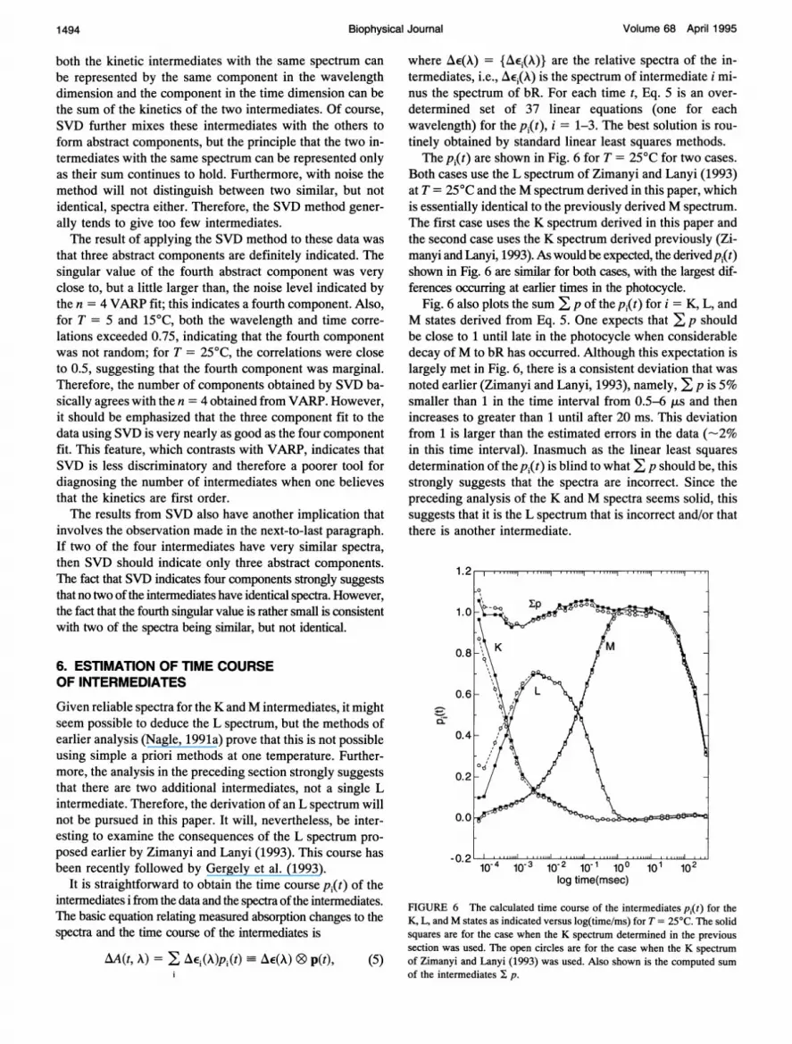
where AE(A) = {AEj(A)} are the relative spectra of the in-termediates, i.e., AEj(X) is the spectrum of intermediate i mi-nus the spectrum of bR. For each time t, Eq. 5 is an over-determined set of 37 linear equations (one for eachwavelength) for the pi(t), i = 1-3. The best solution is rou-tinely obtained by standard linear least squares methods.The p1(t) are shown in Fig. 6 for T = 25°C for two cases.

Both cases use the L spectrum of Zimanyi and Lanyi (1993)at T = 25°C and the M spectrum derived in this paper, whichis essentially identical to the previously derived M spectrum.The first case uses the K spectrum derived in this paper andthe second case uses the K spectrum derived previously (Zi-manyi and Lanyi, 1993). As would be expected, the derivedpi(t)shown in Fig. 6 are similar for both cases, with the largest dif-ferences occurring at earlier times in the photocycle.

Fig. 6 also plots the sum E p of the pi(t) for i = K, L, andM states derived from Eq. 5. One expects that E p shouldbe close to 1 until late in the photocycle when considerabledecay ofM to bR has occurred. Although this expectation islargely met in Fig. 6, there is a consistent deviation that wasnoted earlier (Zimanyi and Lanyi, 1993), namely, E p is 5%smaller than 1 in the time interval from 0.5-6 ,us and thenincreases to greater than 1 until after 20 ms. This deviationfrom 1 is larger than the estimated errors in the data (-2%in this time interval). Inasmuch as the linear least squaresdetermination of thepi(t) is blind to what E p should be, thisstrongly suggests that the spectra are incorrect. Since thepreceding analysis of the K and M spectra seems solid, thissuggests that it is the L spectrum that is incorrect and/or thatthere is another intermediate.

1.2

1.0 P \

0.0

10-4 10-3 10-2 10-1 100 101 102log time(msec)

FIGURE 6 The calculated time course of the intermediates pi(t) for theK, L, andM states as indicated versus log(time/ms) for T = 25°C. The solidsquares are for the case when the K spectrum determined in the previoussection was used. The open circles are for the case when the K spectrumof Zimanyi and Lanyi (1993) was used. Also shown is the computed sumof the intermediates I p.

Biophysical Journal1 494

Testing BR Photocycle Kinetics

The problem in the preceding paragraph was fixed earlier(Zimanyi and Lanyi, 1993) by simply adding enough topL(t)to make E p equal to 1. Because this fix has no theoreticalbasis, a different fix is employed here. If it is assumed thatthe reason that E p is not identically 1 is due to noise, say,in the flash intensity for different measuring times, then avalid fix is simply to normalize E p to 1 (except for the latepart of the photocycle). Also, pK(t) and PL(t) in Fig. 6 os-cillate weakly around 0 for later times, which is clearly justnoise, so it is appropriate to set these to 0. Fig. 7 shows thefixed result. Thesepi(t) are similar to those given earlier (Fig.10 C in Zimanyi and Lanyi (1993) and Fig. 2 in Gergely et al.(1993); the latter study used the earlier spectra but only usedthree wavelengths to determine the p1(t)).

7. INDEPENDENT CRITERION FOR GOODNESSOF SPECTRA

In the last section it was noted that E p is not necessarilyequal to 1 if the spectra are incorrect. This could be a usefulcriterion for improving the spectra, as suggested by Zimanyiand Lanyi (1993). It was attempted to use this simply byscaling the difference spectrum for L; this changed the timeinterval at which E p was less than 1 but did not significantlyimprove its overall deviation from 1. As we also believe thatthere is an additional intermediate, further exploration in thisdirection was not pursued. It must be emphasized, however,that this criterion is not sufficient to determine the spectrauniquely (Nagle, 1991a), i.e., it is possible to have incorrectspectra that will obey this criterion even for the ideal case ofno experimental noise.

In this section a similar criterion will be presented that hasa distinct advantage. To apply the preceding > p = 1 cri-terion requires guessing all the spectra, and when the crite-rion is not met it is unclear which spectrum is incorrect. Thecriterion to be presented now allows each spectrum to betested independently of the other spectra.The basic idea is that the difference spectra AE can be

written as linear combinations of the data AA with coeffi-cients q:

AEi(X) = qi(tj)AA(tj, A). (6)

Of course, this requires that intermediate i be present at leastat one of the times tj; it also requires that the total numberof times nj be greater than or equal to the number of inter-mediates present at the chosen times tj. If the number ofchosen times nj equals the number of intermediates n, thenthe coefficients qi(tj) are uniquely determined unless thespectra are not linearly independent. If nj exceeds n, then theqi(tj) are not uniquely determined. The qi(tj) matrix is es-sentially the inverse of the pi(tj) matrix defined in Eq. 5; bymultiplying Eq. 5 on the left by the q matrix one obtains

qi (tj )=Pk(tj ) = * (7)

Next consider times tj early enough that no decay back tobR has occurred, so that the sum Empm (tj) is 1. Singling out

a particular intermediate k, this may be written as

Pk(tj) = 1 - Pm(tj)-m#k

Substituting Eq. 8 into Eq. 7 when k # i yields

I qi(tj) [1 pm(tj)k = °

j m7&k

(8)

(9)

For each term involving pm(tj) the sum overj vanishes by Eq.7 unlessm equals i and it equals 1 whenm equals i. Therefore,one has

I qi(tj) = 1 (10)

for each intermediate i. Equation 10 is the criterion that must besatisfied by good spectra. The qi(tj) are easily calculated usingleast squares analysis of Eq. 6. The key feature is that all the qifor a given i are calculated from the data AA and from only thedifference spectrum AE(AX) of intermediate i.

This test was applied to putative spectra in the followingway. The data AA(tjk,k) at the first five times were added, aswere the data at subsequent blocks of five times. Only thefirst five blocks of times were used at T = 25°C in order toguarantee that Eq. 8 was satisfied. This meant that the num-ber of effective times was ni = 5. Even though only n = 3or 4 spectra are anticipated, making ni larger than n guar-antees that the spectral space is completely spanned. Thenonuniqueness of the qi does not affect the sum . qi, whichis required for the test in Eq. 10.The result for the M spectrum was Ej qM(tj) = 1.031; this

could be reduced to 1 by choosing a smaller fraction cyclingof 0.148. Because the M spectrum is least controversial, thiscan be considered to be the benchmark for the other spectra.The results for the L and K spectra of Zimanyi and Lanyi(1993) are qL= 0.941 and E qK = 0.942; both are sig-nificantly smaller than for the M spectrum. The result for theK spectrum proposed in this paper is E qK = 0.966, whichis somewhat closer to 1 than the previous result. This is anindependent argument that the present K spectrum is betterthan the earlier one. However, there is still a 6% disagree-ment between E qm and E qK, which suggests that there areother problems with these spectra or with the data or with theassumptions about the photocycle. Similar results were obtainedwhen niwas reduced below 5. Nevertheless, the test suggests thatthe L spectrum is the least reliable, as anticipated.

8. KINETIC MODELS FROMCONCENTRATIONS P,(T)From the time courses p1(t) of the intermediates, a relativelystraightforward method exists to obtain the best kineticmodel (Nagle, 1991a and 1991b), including the determina-tion of which rate constants are nonzero as well as the de-termination of the values of the nonzero rate constants. Themethod begins by assuming nonzero rates for all possibletransitions and the fitting program systematically drives ratessuccessively to zero, thereby simplifying the model. This

Nagle et al. 1 495

Volume 68 April 1995

method was applied for the pi(t) in Fig. 7. Detailed results willfirst be presented for the case with the K spectrum found in thispaper, and differences for the earlier K spectrum will be de-scribed at the end of this section. When only three intermediates(n3) were allowed, the method led to the kinetic model.

0.6

0.4

02.2

10-4 10-3 10-2 10-1 10°0 101 10 2log time(msec)

FIGURE 8 Fits to the time course of the intermediates at 25°C. The solidsquares are the pi(t) from Fig. 7. The dotted-dashed lines show the fit fromthe n3.4a model, and the dashed lines show the fit from the n3.5c modeldescribed in the text. The solid lines show the simultaneous model inde-pendent nonlinear least squares fit using four exponentials.

In the ensuing analysis, one should remember that eachkinetic model fits the pi to special combinations of sums ofn exponentials, so kinetic model fits can not have smaller upthan fits with general sums of exponentials using VARP. Oneway to determine the adequacy of the fit with the n3.4a ki-netic model is to compare the up = 0.035 of the fit with theup = 0.030 obtained by simultaneously fitting the pi(t) datawith sums of three exponentials (with only three apparentrate constants), using VARP. The closeness of these twovalues of up is consistent with n3.4a being the best kineticmodel with n = 3 intermediates.

Fig. 8 also shows the result of simultaneously fitting thepi(t) with sums of four exponentials with only four apparentrate constants, using VARP. The op of this fit is 0.0095,considerably better than for either the n3.4a model or then = 3 VARP fit. This makes it clear that kinetic models withonly n = 3 intermediates are not adequate, even though thepi(t) were biased toward three intermediates by choosingonly three spectra. Increasing the number of exponentials tofive only decreases up to 0.0085, so most of our effort hasbeen on models with n = 4 intermediates.

It is difficult to proceed with an analysis with n = 4 in-termediates from three pi(t) unless it is assumed that thespectrum of the extra intermediate is the same as one of thethree original spectra. If this is assumed, then the sum of twoof the pi(t) determined from a kinetic model must add to oneof the pQ(t) shown in Fig. 8. This assumption and the cor-

responding procedure have been employed by Varo andLanyi (1991a) and Zimanyi and Lanyi (1993) and by Gergelyet al. (1993) for absorption data for the photocycle andby Nagle (1991b) for the analysis of Raman data. These

1.0

0.8

K *->L

(11)M -> bR,

which may be more succintly and equivalently written asK *-- L + K -> M -- bR. This model has four rate constantsand places L on a dead-end side path. We will call this then3.4a model, where the final letter is different for other mod-els with three intermediates and four rate constants. The fitto the pi(t) for this model is shown in Fig. 8 by the dotted-dashed lines. The uTp of the fit for the n3.4a model is 0.0354.The subscriptp on af emphasizes that this is the fit to the pi(t)and not to the data, so orp is not to be compared to the oJ'sin Section 4. It is also straightforward to calculate the fits tothe data from the pi(t) and the relative spectra using Eq. 5.The sigma of this fit will be called Cod. For the n3.4a model(d= 1.43 mOD, which is somewhat poorer than the of = 1.1mOD obtained from fitting three exponentials in Section 4.The n3.4a model is somewhat unconventional in that L is

not on the path from K to bR but lies on a cul-de-sac. It istherefore of interest to examine the model (n3.5c):

K <-> L <-> M ---> bR. (12)The fit for this model is shown in Fig. 8 by dashed lines. Theup for this n3.5c model is 0.0559. Also, Cd = 2.04 mOD forthis model, so the n3.5c is clearly a considerably poorermodel than the n3.4a model.

1.0

K0.8 M

-o L

0.6

80.4

0.2-

0.0

-0.2 -. ,. -..,10-4 10-3 10-2 10.1 100 101 102

log time(msec)

FIGURE 7 Same as Fig. 6 except that the p1(t) have been normalized sothat their sum equals 1 for times less than 7 ms. Also, pK(t) has been setto 0 after 0.25 ms and pL(t) has been set to 0 after 2.3 ms.

1 496 Biophysical Journal

4-

Testing BR Photocycle Kinetics

previous analyses have shown that models with two M statesclearly fit the pi(t) better than models with only one M andone less intermediate.With the assumption that there are n = 4 intermediates

and two M states, two models have been found that fit thedata nearly equally well, the n4-2M.7b model

K ->L ->M1 M2-- bR + K <-M1 (13)with (Jp = 0.01781 and Yd = 0.990 mOD and the n4-2M.7a model

K*-> L*-> Ml K + K-> M2-* bR (14)with up = 0.01778 and 0rd = 0.984 mOD; these ad maybe compared with the oa = 0.49 obtained from fitting fourexponentials using VARP. Both models require onlyseven independent rates because the K <- Ml backreac-tion is uniquely related to the other rates involving K, L,and Ml. The dashed curves in Fig. 9 show the best fit forthe n4-2M.7b model. This fit is clearly superior to the fitsfor the n = 3 models in Fig. 8. The n4-2M.7a model israther unorthodox in having a cul-de-sac loop K *-- L *->Ml 1-> K involving two intermediates, L and Ml, that areoff the main pathway. The n4-2M.7b model is rathermore orthodox and would be identical, if the K *-> Ml pathwere removed, with the model preferred by Zimanyi andLanyi (1993), which we will call the n4-2M.6 model,

K -L ->M1-M2---bR. (15)A fit was performed to the n4-2M.6 model and yieldedup of 0.02268 and Ud = 1.135 mOD. Although the n4-

0-Q-t

10i4 10-3 10-2 10-1 100 101 102log time(msec)

FIGURE 9 Fits to the time course of the intermediates at 25°C assumingfour intermediate states. The solid squares are the pQ(t) in Fig. 7. The dashedlines show the fit assuming two M states, model n4-2M.7b; PM1 and pM2 as

well as PM1 + pM are shown. The solid lines show the fit assuming two Lstates, model n4-2L.6; PL1 and pL2 as well as PL1 + pL2 are shown.

2M.6 model has one fewer independent rate constant thanthe n4-2M.7b model, the K <-> Ml path is statisticallysignificant using an F-test (Nagle, 1991b). Even the fit tothe n4-2M.7b model indicates systematic discrepanciesfrom the pi(t), as seen in Fig. 9 and as indicated bythe crp = 0.0178 being nearly twice the up = 0.0095 ofthe fit by sums of four exponentials.An attempt was also made to find a kinetic model with two

L states. This was not expected to be successful because ithad not helped much when dealing with Raman data (Nagle,1991b); the result was rather surprising. The best fittingmodel with two L states, called n4-2L.6,

K <-> Li *-> L2 + K -- M bR, (16)

has orp = 0.01126, od = 0.742 mOD, and only six indepen-dent rates. The fit to the pi(t) is shown by solid lines in Fig.9 and is clearly superior to the fit from the n4-2M.7b model.At this point this model is clearly the best one with fewer thanfive intermediates.

Further testing involves investigation of some of thechoices not taken. The first of these is the use of the K spec-trum from Zimanyi and Lanyi (1993) instead of the K spec-trum derived in this paper and the alternative pi(t) shown inFig. 7. The general conclusions regarding which is the bestmodel continue to hold. The two M models n4-2M.7a andn4-2M.7b both have o(p = 0.0268 (compared to 0.0178 pre-viously). The favored two L model n4-2L.6 has up =0.01948 (compared to 0.01126 previously), and this wasagain the best fitting model. However, all kinetic models fitmuch more poorly to these pi(t) functions as seen by com-paring the op of the fits. It is even more remarkable that thesimultaneous four exponential fit to these pi(t) has op =0.00841, slightly better than for thepi(t) analyzed above. Theinterpretation of these poorer fits using kinetic models incontrast to the equally good fit using general sums of ex-ponentials follows from the fact that the sums of exponentialsgiven by all possible kinetic models is a subset of generalsums of exponentials. Therefore, an incorrectly derived setofpi(t) could be nicely fit with a general sum of exponentialsbut poorly fit with even the best kinetic model. Inasmuch asthe only difference in deriving the two sets of pi(t) was theK spectrum used, this is additional evidence that the K spec-trum derived in this paper is significantly superior to the oneobtained previously.At the lower temperatures T = 5 and 15°C the pi(t) were

not so well behaved as at 25°C, with clearly spurious nonzerovalues of PK and PL at late times. Perhaps as a consequence,none of the fits to any model was as good for these tem-peratures, and clear distinctions were not apparent. However,the n4-2L.6 model remained about as good as any othermodel, even though the best orp and (d were approximatelytwice as large as the up and ad, respectively, obtained fromfitting simultaneously to four exponentials. Also, the indi-vidual rates were reasonably consistent with Arrhenius be-havior as a function of temperature.

Finally, we limited our tests of models with five inter-mediates to one specific model that has two L and two M

Nagle et al. 1 497

Volume 68 April 1995

states. This model, discussed previously (Zimanyi and Lanyi,1993), will be called the nS-2L2M.8 model:

K -Ll*-> Ml-M2--> bR + M1*->L2. (17)

One unusual feature of this model is that the best Li *-* Mlrates given by the fit are very fast compared to all other rates.At 25°C the fitted crp is marginally smaller by 0.0001 thanfor the n4-2L.6 model, but for the lower temperatures (Tp is-0.001 greater than for the n4-2L.6 model. While thismakes the n5-2L2M.8 model slightly inferior, it is a veryclose alternative model.

9. ALTERNATIVE APPROACH TO KINETICMODELS AND SPECTRA

It was clear from the process of obtaining the time course ofthe intermediates pi(t) that there are inherent difficulties inobtaining all the spectra involved, especially when there areclearly more than three intermediates. This suggests that itis worth considering the alternative approach to photocyclekinetics that does not try to obtain the spectra first (Nagle,1991a; Lozier et al., 1992). Although this approach mustassume that the spectra are independent of temperature, theK andM spectra derived earlier in this paper indicate that thisis a reasonable assumption.The difficulty with this alternative approach is that there

are local minima in the global nonlinear least squares fittingspace, so the result of the search depends upon the initialguess and therefore may not find the best solution. Also, ashas been discussed (Nagle, 1991a), with even modest non-zero noise levels it may not be possible to distinguish the"true" solution from spurious solutions that fit the data aboutequally well. This is likely to be a serious problem for thepresent data, which have a signal-to-noise ratio of only-100:1. This is some five times less than the signal-to-noiseratio of previous data (Xie et al., 1987) for which the methodwas not successful, especially in producing reasonable spec-tra, although it must be remembered that the full photocycleis complicated by having many more intermediates and thatthe K spectra produced independently from those data werenot as independent of temperature as the present data. Never-theless, this method should at least be able to determine whethercertain models are distinctly inferior to other models.

Results of applying the alternative method to the T = 5,15, and 25°C data simultaneously were obtained under theassumption that each fundamental reaction rate obeyed asimple Arrhenius relation. When applied to the n4-2L.6model, the oa of the fit to the data was 0.8124 (which shouldbe compared with VARP fits of 0.46-0.63 for different tem-peratures); this was the smallest a of all the models tried. Thetwo L spectra were blue shifted approximately 10-20 nmfrom bR, but the relative spectra were much too large near540 nm and too strongly negative near 400 nm. For com-parison, the n4-2M.6 model has a cr = 0.8128 with reason-able L and M2 spectra, but with an Ml spectrum that is muchtoo large near 410 nm and much too negative near 570 nm.

K <-> Li <-> M -- bR + Li <-> L2 + weak L2 *-> M; the L2spectrum, however, is more M-like than L-like, and a =

0.8239. The alternative method therefore does not yieldmuch new information about the D96N photocycle fromthese data, except to confirm that several models are equallyconsistent with the data.

Systematic experimental errors in the data could also ac-count for difficulties in obtaining good results from thismethod. A number of systematic errors were discussed byXie et al. (1987). One that was realized subsequently (Lewisand Kliger, 1991) concerns data taken with magic angle po-larization, which are subject to an artifact not present in par-allel plus two times perpendicular data. Although this artifactbecomes negligible in the limit of dilute samples, perhaps theintermediate optical density for these D96N samples is suf-ficiently high to complicate the rather delicate analysis re-quired by this method.

1 0. DISCUSSION

The D96N mutant of bR is particularly favorable for pho-tocycle studies. An excellent M spectrum was obtained pre-viously (Zimanyi and Lanyi, 1993). The somewhat simplermethod in this paper confirms thisM spectrum as well as thefraction cycling at 25°C. It is particularly pleasing, in con-trast to earlier studies, that the M spectrum has a singlepeak in the blue and zero absorbance above 500 nm (seeFig. 3). The feasibility of this analysis is due to the slowdecay of M and the lack of any other late intermediates,such as N and 0.

This paper shows how the difference spectrum of the firstintermediate, which is K for these data, can be obtained byglobal nonlinear least squares methods (VARP). Using thefraction cycling obtained by the determination of theM spec-

trum, an improved K spectrum is obtained (see Fig. 5). Theprevious K spectrum (Zimanyi and Lanyi, 1993) was con-

siderably less well determined by the three filter method thanthe M spectrum, so it may not be too surprising that there are

real differences compared to the new K spectrum.An important result from the K and M difference spectra

is that both are consistent with negligible temperature de-pendence between 5 and 25°C because the difference spectraat all temperatures can be scaled to the same difference spec-

trum for each intermediate. Complete proof of temperatureindependence would require obtaining the fraction cycling atthe lower temperatures; this is not reliable even for the D96Nphotocycle. However, the values of the fraction cycling at 5and 15°C required for temperature independence are rea-

sonable; also, it would be unlikely that temperature depen-dence, which involves a multidimensional functional basis,would be duplicated by a one-dimensional variable such as

the fraction cycling. Although the true rate constants and thekinetic photocycle change dramatically from 5 to 25°C, thespectra of the true chemical intermediates would not be ex-

pected to vary any more than the negligible temperature variationof noncycling bR. Thus, the K and M spectra presented here are

The model that gives the most reasonable looking spectra is

1498 Biophysical Journal

likely to be the spectra of true chemical intermediates.

Nagle et al. Testing BR Photocycle Kinetics 1499

The temperature independence of the K and M spectrasupport the key assumption used in an ab initio method forphotocycle analysis (Nagle, 1991a; Lozier et al., 1992).However, this method demands very accurate data, and aconvincing derivation of the best kinetic model with accept-able spectra has not been achieved. Therefore, more attentionhas been paid in this paper to the alternative method ofZimanyi and Lanyi (1993).A necessary step in any method of determining the pho-

tocycle is the determination of the number of chemical in-termediates (Xie et al., 1987). Simple nonlinear least squaresfitting of sums of exponentials to the data (VARP) stronglyconfirm that there are more than three intermediates, whichwas suspected previously (Zimanyi and Lanyi, 1993), andsuggests that there are most likely four intermediates. Sin-gular value decomposition is also consistent with the pres-ence of a fourth component, although the fourth componentis more marginal than for VARP fitting, consistent with thepossibility that two of the spectra may be similar.

Even if there had been only three intermediates, rigoroussolution of the photocycle is not possible because of uncer-tainty in the third, L, spectrum. With two intermediates inaddition to the well-determined K and M, the problem is agood deal harder. However, since the three filter methodworked very well for the M spectrum and not too badly forthe K spectrum, it is reasonable to consider the L spectrumobtained previously and to suppose that the fourth spectrumis the same as L or M. Using these three spectra allows astraightforward calculation of the time course pi(t) of theintermediates from the data. As noted previously (Zimanyiand Lanyi, 1993), however, the sum of the pi(t), i.e., thefraction cycling at time t, did not decrease monotonically asrequired. This indicates some difficulties in the spectra. (SeeSection 6.) To try to pinpoint which spectrum is most likely tobe the problem, a new criterion was developed (Section 7) thatindicates that the L spectrum is the least reliable, although therewere also inconsistencies between the M and K spectra.From the time course pi(t) of the intermediates, it is com-

putationally easy to obtain the best photocycle if it is assumedthat there are three intermediates, K, L, and M, as shown inSection 8. This model is somewhat unusual in that L is ona cul-de-sac. However, the greatly improved fit to the datawith four exponentials discussed above requires consider-ation of a photocycle with four intermediates; this conclusionis further reinforced by the great improvement in the non-linear least squares fit to the pi(t) with four exponentialscompared to three.Both visible spectroscopy (Varo and Lanyi, 1991a) and

Raman spectroscopy (Nagle, 1991b) indicate that theminimal photocycle for native bR has intermediates K, L,Ml, M2, N, and 0. Inasmuch as there are no N and 0intermediates in the D96N mutant, the most likely sug-gestion would be that the fourth intermediate would be asecond M state. It was therefore rather surprising that thekinetic model that gives the best fit for the D96N pho-tocycle has two values of L both of which are on a single

cul-de-sac. This purely analytical result is not one that wefind very appealing or understandable, although onemight keep in mind that the early part of the photocycleof the D96N mutant could be less straightforward than forthe wild type. Perhaps, in view of the assumptions anduncertainties in the spectra required to obtain the timecourse of the intermediates, this result should not be givenmuch consideration. A close alternative is the n5-2L2M.8model, which has a second extra intermediate and twoextra rates but which is statistically almost as good as then4-2L.6 model. Choosing between two such alternativesor more complicated models not considered in this papermay involve physical modeling of the mechanism of thephotocycle. Even though a complete understanding of thephotocycle of bR, even for this mutant, remains a chal-lenge, the methods in this paper enable the choice to bebetter focused to a few models.

The efforts of Drs. Zimanyi and Lanyi were supported by NIH grantGM29498 to J.K.L.

REFERENCESBevington, P. R. 1969. Data Reduction and Error Analysis for the Physical

Sciences. McGraw-Hill, New York.Gergely, C., C. Ganea, G. Groma, and G. Varo. 1993. Study of the pho-

tocycle and charge motions of the bacteriorhodopsin mutant D96N.Biophys. J. 65:2478-2483.

Golub, G. H., and R. J. Leveque. 1979. Extensions and uses of the variableprojection algorithm for solving nonlinear least squares problems", Proc.Army Numerical Analysis and Computing Conference, ARO Report.79-3:1-12.

Hessling, B., G. Souvignier, and K. Gerwert. 1993. A model-independentapproach to assigning bacteriorhodopsin's intramolecular reactions tophotocycle intermediates. Biophys. J. 65:1929-1941.

Lewis, J. W., and D. S. Kliger. 1991. Rotational diffusion effects onabsorbance measurements: limitations to the magic angle approach.Photochem. Photobiol. 6:963-968.

Lozier, R. H., A. Xie, J. Hofrichter, and G. M. Clore. 1992. Reversible stepsin the bacteriorhodopsin photocycle. Proc. NatL. Acad. Sci. USA. 89:3610-3614.

Lozier, R. H., R. A. Bogomolni, and W. Stoeckenius. 1975. Bacteriorho-dopsin: a light-driven proton pump in Halobacterium halobium. Biophys.J. 15:955-962.

Nagle, J. F. 1991a. Solving complex photocycle kinetics: theory and directmethod. Biophys. J. 59:476-487.

Nagle, J. F. 1991b. Photocycle kinetics: analysis of Raman data from bac-teriorhodopsin. Photochem. Photobiol. 54:897-903.

Nagle, J. F., L. A. Parodi, and R. H. Lozier. 1982. Procedure for testing kineticmodels of the photocycle of bacteriorhodopsin. Biophys. J. 38:161-174.

Schrager, R. I. 1984. Optical spectra from chemical titration. Siam J. Alg.Disc. Meth. 5:351-358.

Varo, G., and J. K. Lanyi. 1991a. Kinetic and spectroscopic evidence foran irreversible step between deprotonation and reprotonation of the Schiffbase in the bacteriorhodopsin photocycle. Biochemistry. 30:5008-5015.

Varo, G., and J. K. Lanyi. 1991b. Thermodynamics and energy coupling inthe bacteriorhodopsin photocycle. Biochemistry. 30:5016-5022.

Xie, A. H., J. F. Nagle, and R. H. Lozier. 1987. Flash spectroscopy of purplemembrane. Biophys. J. 51:627-635.

Zimanyi, L., and J. K. Lanyi. 1993. Deriving the intermediate spectra andphotocycle kinetics from time-resolved difference spectra of bacterior-hodopsin: the simpler case of the recombinant D96N protein. Biophys. J.64:240-251.