1

Testing the balanced growth hypothesis: Evidence from China

Hong Li* and Vince Daly, Kingston University

Abstract

We investigate whether China’s experience during 1952-2004 supports the balanced growth

entailment of the neoclassical growth model. Estimation of long-run relations among output,

consumption and investment for the full period reject the balanced growth hypothesis for both

the national and regional economies. When the economic reforms of the late 1970s are

modelled as a structural break by the methods of Johansen et al. (2000) and Perron (1989), we

find some evidence of balanced growth in the pre-break period but in the post-break period

the ‘great ratios’ are trend-stationary, precluding fully balanced growth, though permitting a

common (stochastic) productivity trend.

JEL classifications: C32, E13, O53

Keywords: balanced growth, great ratios, cointegration, structural breaks

* corresponding author. We are grateful for advice received from colleagues.

2

Testing the balanced growth hypothesis: Evidence from China

1 Introduction

Kuznets’ (1942) study of the macroeconomic aggregates of the USA during that country’s

period of industrialisation led him to posit a long-run constancy in the ratio of savings to

income. Klein and Kosobud (1961) applied more formal trend-fitting methods to Kuznets’

data and concluded that some of the ‘great ratios’ were constant but others, including

savings/income, actually possessed a slight trend. At the same time Kaldor (1961) posited a

number of constancies, though not including the savings/income ratio, as “stylised facts” of

the growth process. These empirical observations helped to launch what has been called the

“balanced growth” literature, characterised in King et al. (1991, p819) as claiming empirical

support for ‘… balanced growth in which output, investment and consumption all display

positive trend growth but the consumption:output and investment:output “great ratios” do

not ....’

This paper investigates the extent to which the balanced growth hypothesis is applicable to the

development of the Chinese economy since the middle of the last century. During this period

the political institutions have been such that the central government of China has been able to

initiate radical structural change; we focus particularly upon the reduction of central planning

that was initiated in the late 1970s. Following these economic reforms, China has sustained

high economic growth – in marked contrast to the pre-reform decades. Overall, this is a

qualitatively different context to that of the USA, which provided an empirical underpinning

to the initial balanced growth propositions. We examine whether such propositions remain

3

applicable if transferred from the USA experience to that of China. The question is of more

than purely academic interest since the presence of balanced growth speaks for, rather than

against, the relevance of the neoclassical growth model – which is a model offering relatively

little opportunity for government to play a significant role in the growth process.

The neoclassical growth model predicts a balanced growth path along which per capita

output, consumption and investment grow at the same constant rate while the

investment/output and consumption/output ratios are constant. This hypothesis has not been

consistently supported by empirical investigation using data from developed countries. King

et al. (1991), using cointegration analysis, find that post-war U.S. macroeconomic data

exhibit a common stochastic trend, satisfying parameter restrictions consistent with the

balanced-growth hypothesis. Mills (2001) uses the technique of generalised impulse response

functions as well as Johansen’s method for estimating cointegration rank, and finds evidence

to support the stationarity of the ‘great ratios’ for the UK during the post-war period. On the

other hand, Kunst and Neusser (1990), using Johansen’s method, strongly reject the

hypothesis of stationary ‘great ratios’ for Austrian data. Serletis (1994) does not find any

evidence of stationary ratios in multivariate analysis of Canadian data (1929-1983).

Furthermore, Serletis and Krichel (1995) and Harvey et al. (2003) do not find evidence from

OECD and G7 countries, respectively, to support the hypothesis of balanced growth.

Importantly, from the perspective of this paper, Clemente et al. (1999) argue that the evidence

against balanced growth is less convincing when the possibility of structural breaks is taken

into account.

In the light of the mixed empirical results in the literature, we are motivated to examine the

empirical support for the balanced growth hypothesis in a developing country, in particular

4

China, as opposed to the advanced industrialised countries. The case of China is of particular

interest due to the noticeable change in the pace of economic growth following economic

reforms and also because of the diversity in the regional economies. The regime switch and

the lack of uniform development across China’s regions (Li and Daly, 2005), both allow us to

explore whether the evidence for balanced growth varies with the level of development.

This empirical study is underpinned by the neoclassical stochastic growth theory developed

by Brock and Mirman (1972), Donaldson and Mehra (1983) and implemented empirically by

King et al. (1988). Following King et al. (1991), Serletis (1994) and Serletis and Krichel

(1995), we investigate the Chinese growth process via multivariate analysis of major

macroeconomic aggregates and also univariate analysis of selected ‘great ratios’. Specifically,

we apply Johansen’s (1995) maximum likelihood approach to estimate the number of long-

run steady-state relations among Chinese per capita output, consumption and investment, at

the national and regional levels and to test the validity of the parametric restrictions that

characterise balanced growth. Our novel contribution to the empirical testing of balanced

growth is that we extend the cointegration analysis to allow for structural change by using the

method of Johansen et al. (2000). We further use Perron’s (1989) approach to incorporating a

structural break in univariate unit-root testing, allowing us to assess whether the log ratios of

consumption vs. output and investment vs. output are stationary – as is required by the

hypothesis of balanced growth. The following questions will be examined. Are the time series

properties of Chinese national and regional per capita output, consumption and investment

properties consistent, in whole or in part, with the balanced-growth predictions of the

neoclassical growth model? Does the level of development affect the evidence for balanced

growth? Are the conclusions sensitive to the inclusion/exclusion of a structural break to

recognise the major economic reforms of the late 1970s?

5

The paper is organised as follows. Section 2 summarises the neoclassical growth theory and

its econometric representation; section 3 describes the data and conducts a preliminary

analysis of their time series properties; section 4 applies the standard Johansen framework to

determine whether the Chinese macroeconomic variables possess cointegrating vectors in

number appropriate for balanced growth and whether these vectors additionally satisfy the

parameter restrictions required for stationarity of the ‘great ratios’. Section 5 extends the

analysis by using the methods of Johansen et al. (2000) and Perron (1989) to take into

account the possibility of a structural break caused by the economic reforms of the late 1970s.

Section 6 concludes.

2 Theoretical considerations and econometric representation

The Solow and Swan (non-stochastic) growth theory for a one-sector economy specifies a

neo-classical production function exhibiting constant returns to scale and diminishing

marginal product with respect to each input. The model assumes that technology augments the

labour input to an extent which grows at an exogenously fixed rate, g. Fixed capital formation

is provided by a constant fraction, s, of unconsumed output. Production technology and

consumer preferences are assumed to be such that a steady state solution exists. The steady-

state per capita quantities: per capita capital, k; per capita output, y; and per capita

consumption, c, then all grow at the same rate as technological progress. Their aggregate

levels, K, Y and C, grow accordingly in the steady state at a common rate of g+n, where n is

an exogenously determined rate of growth for the size of the labour force.

In the particular case of the Cobb-Douglas production function we have

6

αα )(1

tttt LAKY−= (1.)

At represents exogenous labour-augmenting technical progress. The constant growth rate for

the effectiveness of labour can be represented as a deterministic logarithmic trend:

( ) ( )1loglog −+= tt AgA . The per capita variables all grow at the exogenously given rate of

technical progress: gAky

=== γγγ ( ( ) ( )1loglog −−≡ ttx xxγ , ttt LXx = ). This “balanced

growth” of the per capita aggregates implies that the ‘great ratios’ of investment and

consumption to output are constant.

Alternatively, technological progress can be modelled stochastically (King et al., 1988) as a

logarithmic random walk with drift:

( ) ( ) ttt AgA ε++= −1loglog (2.)

The term, εt, is a white noise process representing productivity shocks, i.e. deviations of the

growth rate for labour effectiveness from its expected value, g. Each εt contributes a

permanent impact: their cumulative effect at any point in time is their undiscounted sum up to

and including that date, which is a ‘stochastic trend’. In the solution path for a log-linear

version of the stochastic growth model the logarithms of output, consumption and investment

consequently all share this stochastic trend (King et al., 1988). These three aggregates are

therefore individually non-stationary, being integrated of first order - ( )1I . Nevertheless,

because they have in common a single stochastic trend, it is possible to construct two distinct

‘cointegrated’ linear combinations of them that are stationary. The model solution further

implies that these combinations are the logarithms of the consumption / output and

investment / output ‘great ratios’, i.e. there is balanced growth in a stochastic sense. The

7

testable implications of the model then include (1) an appropriate cointegration rank and (2)

parametric restrictions to ensure that the cointegrating vectors imply stationarity of the ‘great

ratios’. The required cointegration rank, r, for an error-correction model in the logarithms of

per capita output, consumption and investment is r = 2. For the cointegrating vectors to imply

“balanced growth”, their normalised coefficients should be ( )011 − and ( )101 − , and

there should be no trend in the cointegration space. These restrictions can be tested within the

Johansen (1995) framework or alternatively by directly assessing the stationarity of the ‘great

ratios’.

3 Data: sources and characteristics

The raw data used in this study are those of GDP, final consumption expenditure, gross fixed

capital formation, consumer price index and population between 1952 and 2004, provided at

provincial level in The Gross Domestic Product of China 1952-19951 and various issues of

the Statistical Yearbook of China published by the State Statistical Bureau of China. We

combine Sichuan and Chongqing2 as a single province and omit Tibet due to its incomplete

data availability. This yields data series for 28 provinces, at annual frequency, which are then

aggregated to regional level, as described below, to compile the variables of interest.

The variables of interest in this study are real per capita GDP, real per capita consumption

expenditure and real per capita fixed capital formation at national and regional levels. These

variables are constructed as follows. First, the provincial series for GDP, final consumption

1 This is compiled by the Department of National Economic Accounting, State Statistical Bureau and published

by Dongbei University of Finance and Economics Press

2 Chongqing was separated as a province from Sichuan in the early 1990s.

8

expenditure and gross fixed capital formation are converted from nominal to real units by

division by their respective provincial consumer price index. Regional series for the major

administrative regions - Eastern, Central and Western, are then formed by aggregation across

the provinces assigned to each region. National series are produced by aggregation of the

provincial series directly. Similar regional and national aggregation is performed upon the

provincial population data in order to construct series for real per capita output (y), real per

capita consumption (c) and real per capita investment (i) at national and regional levels.

In this section, we examine the time series properties of these per capita series at the national

and regional levels. Figure 1 shows that over time the three variables, in logarithms: logy,

logc and logi, have increased at both national and regional levels of aggregation. An upward

trend had become obvious since the late 1970s, prior to which the series were more volatile

and possibly tended to decline. On the basis of graphical inspection, the three aggregates seem

to share similar trend tendencies. We would like to test more formally whether or not the

series share a common stochastic trend, as is implied by the balanced growth conclusions of

the stochastic neoclassical growth model.

[Figure 1 is about here.]

To implement the formal cointegration tests within the Johansen framework, we first need to

establish that the national and regional logy, logc and logi are ( )1I series. We use the

augmented Dickey-Fuller test, including a constant and trend in the test equations. The lag

length is determined using downward testing beginning with an arbitrarily large number of

lags, in this case 10, on the basis of a modified Akaike Information Criterion (Ng and Perron,

2001).

9

[Table 1 is about here.]

The test results presented in Table 1 indicate that these series may be treated as ( )1I , with the

exception of logc in the Eastern region and nationally – which show evidence of being ( )2I .

We proceed nevertheless, because ( )2I behaviour of consumption does not rule out partially

balanced growth, with stability of the investment/output ratio, and also because of our interest

in the possibility of structural breaks. (This apparent ( )2I behaviour may be seen as

signalling a structural break in the Eastern region – where post-liberalisation growth has been

relatively rapid, and consequently nationally.) Having established that the per capita variables

show evidence of possessing stochastic trends, we move to consider below whether these are

idiosyncratic or shared in common – the latter being a necessary condition for “balanced

growth”.

4. Testing for balanced growth without a structural break

In the absence of cointegration, logy, logc and logi – for a particular region or nationally, are

driven by three separate stochastic trends, precluding balanced growth. We use Johansen’s

(1995) approach to estimate the number of cointegrating vectors constraining the long-run

behaviour of these series. The existence of two cointegrating vectors involving three series

would imply that the series share in common a single stochastic trend, introducing the

possibility of balanced growth. The results of this cointegration analysis are reported in Table

2. Because the presence of a linear trend within a cointegrating relationship would rule out

balanced growth, we use the test variant in which linear time trends are permitted within the

10

data series but not within the cointegration space. Lag lengths in the test VECMs were

selected by sequential modified LR test statistics and found to be 2 or 3 for all cases.

[Table 2 is about here.]

Cointegration analysis suggests that logy, logc and logi share a common stochastic trend in

the Central region and also in the Western region, satisfying a necessary, but not sufficient,

condition for balanced growth in those regions. Nationally, however, and in the Eastern

region the standard Johansen procedure suggests a single cointegrating vector, which imposes

insufficient constraint upon the long run behaviour of the three time series for log(c/y) and

log(i/y), which are the ‘great ratios’ in logarithmic form, to both be stationary. This result

should be interpreted in the context of the previous diagnosis that logc ~ I(2) at the national

level and in the Eastern region. As is argued more completely in Everaert (2003), an I(2)

series – here logc, cannot form a stationary combination with two I(1) series – here logy and

logi. The cointegration space is then two-dimensional, rather than three-dimensional, so that

the cointegration rank must be zero or unity to be consistent with the previous diagnosis that

logy, logi are I(1) series. A cointegration rank of unity for Eastern and national data then

leaves open the possibility that one ‘great ratio’, log(i/y), is stationary but not both.

It is not surprising to discover similar diagnoses of series characteristics at the national level

and in the Eastern region since the Eastern region accounts for the largest proportion of the

Chinese economy. The diagnosis of I(2) behaviour in the Eastern and national logc might be

evidence of a permanent feature, such as a drift in the average propensity to consume, that

precludes balanced growth. Alternatively, it might point to the existence of a structural break

in the series, with logc ~ I(1) on either sided of the break and leaving open the possibility of

11

balanced growth before and/or after the break. As is well known, the Eastern region was

selected to lead the process of economic development following the market liberalisation

reforms of the late 1970s. The Eastern region has consequently experienced the most radical

structural break between the first and second halves of the data period and it may be that this

structural break is mis-interpreted by the standard Johansen procedure as a second unit root

process in the Eastern region, hence also at the national level. The possibility of modifying

the standard procedure to explicitly incorporate a structural break within the cointegration

analysis will be investigated in the next section.

Now we examine the extent of empirical support for the further implication of the

neoclassical stochastic growth theory that the ‘great ratios’ should be stationary stochastic

processes. This can be interpreted, within the Johansen framework, as a requirement that the

normalised coefficients of the cointegrating vectors for logy, logc and logi should be

( )011 − and ( )101 − . We carry out likelihood ratio tests to assess whether these

restrictions are acceptable, individually or simultaneously, given the cointegration ranks

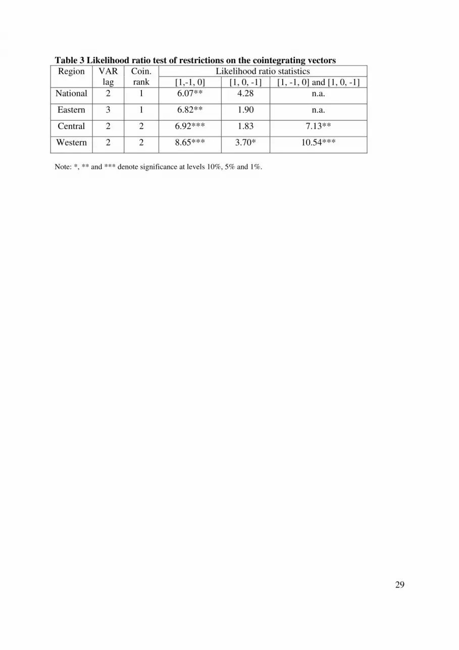
reported in table 2. The results are presented in Table 3.

[Table 3 is about here.]

Table 3 shows that, at national level and in all three regions, the data does not support the

parameter restrictions required for stationarity of log(c/y). In this sense, the balanced growth

hypothesis is rejected even where the cointegration rank is appropriate to it.

Balanced growth, in the sense of the stationarity of log(c/y) and log(i/y) could also be assessed

outside of the Johansen framework by directly investigating the stationarity of these two

12

series via unit-root testing. ADF test results (available on request) agree with the parameter

restriction tests in that they suggest non-stationarity for both of these series in all three

regions. At the national level the unit root null hypothesis is rejected for both series if the

ADF test equation is permitted to include a linear trend, but such a trend then implies

deterministic non-stationarity for the series being tested and thus still precludes balanced

growth in the strict sense of constant means for the ‘great ratios’.

5. Testing for balanced growth in the presence of a structural break

In section 4, we found that Johansen’s method rejects balanced growth, nationally and in all

three regions individually - either because the macroeconomic series do not share a common

stochastic trend, or, where they do so, because the cointegrating vectors do not satisfy the

required parameter restrictions. Direct unit root testing of the ‘great ratios’ gave no grounds to

question this overall dismissal of the possibility of balanced growth.

We noted in passing that the economic reforms of the late 1970s could be seen as implying a

parametric structural break in a VECM representation of the data series. Such a structural

break can undermine the reliability of statistical methods that do not admit its presence.

Accordingly, in this section, we employ alternative statistical methods that allow us to include

a structural break in the analysis, in case this might change the conclusions with respect to the

existence of balanced growth in the pre-reform and/or post-reform periods.

The graphs (Figure 1) of the national and regional log per capita consumption, output and

investment offer visual support for the possibility of a break in trend behaviour around 1978,

when the economic reforms started. We use the method developed by Johansen et al. (2000)

13

to estimate the cointegration rank in the presence of broken linear trends in the individual

series and additionally use Perron’s (1989) method to test for the stationarity of log(c/y) and

log(i/y) in the presence of such a structural break.

Johansen et al. (2000) divide a sample of T observation points into q sub-periods by

exogenous selection of break-points, qjT j L,2,1,0; = , with 10 =T and TTq = . The

maintained model is a levels VAR of order k, hence a VECM of order k-1, in a p-vector of

jointly endogenous variables. The first k observations of each sub-period are reserved as

initial values, so that for each instance of qj L,2,1= the observation points

jj TtkT ≤≤++− 11 are described by

[ ]tit

k

i

ij

t

jt Xt

XX εµπ +∆Γ++

Π=∆ −

−

=

− ∑1

1

1 (3.)

Only the p-vectors of parameters relating to the deterministic components - jj µπ , , may vary

between sub-periods. Cointegration is represented, as in the standard Johansen framework, by

the restriction βα ′=Π , where α and β are rp × matrices. The possibility of quadratic

trends for the levels series is eliminated by the additional maintained assumption that

jj αγπ = in each sub-period.

The models for the separate sub-periods can be written jointly by defining dummy variables:

qjotherwise

TtiffD

j

tj L,2,1,0

1 1

, = =

=−

and

14

qjotherwise

TtkTiffDE

jj

TT

ki

itjtj

jj

L,2,1,0

11 1

1

,,

1

= ≤≤++

==−

−

+=

−∑−

Each tjD , is an indicator for the end of the (j-1)th

sub-period and its lagged values therefore

point to the individual observation points within the jth

sub-period. By summing these lagged

values tjE , acts as an indicator dummy for an entire sub-period. Using these dummy

variables, the separate sub-period models can be combined into one as follows.

t

k

i

q

j

itjijit

k

i

it

t

t

t DXEtE

XX εκµ

γ

βα ∑∑∑

= =−−

−

=

−++∆Γ++

′

=∆

1 2

,,

1

1

1 (4.)

Here µ contains the intercept coefficients for the q sub-periods, and the terms itjij D −,,κ are

included to ensure that the estimation of the parameters of interest is not influenced by data at

the initial observation points within each sub-period.

The time plots in Figure 1 are visually supportive of the possibility that the Chinese series

experienced a break in trend at 1978, associated with the significant reforms to economic

institutions. Since 1979, GDP, consumption and investment appear to have been trending

upwards, in contrast to the preceding years. There is some visual evidence of other disruptive

events, most notably the ‘Great Leap Forward’ of 1958-61, but since our focus is on the

possible impact of the economic reforms that commenced around 1978, we set q=2, with

T0=1952, T1=1978 and T2=2004.

The cointegration rank is estimated by a variant of the canonical correlations approach of

Johansen (1995, Ch.6). Johansen et al. (2000) present a table, based on response surface

15

analysis, which enables the investigator to select appropriate parameters for a gamma

distribution to be used for setting the critical values of the relevant test statistics. The

parameters of the gamma distribution vary according to the number and location of sample

break-points; in our case, with a single break-point, v = T1/T2 =0.4717 is a key ratio for

determining these parameters. Our results are reported in Table 4.

[Table 4 is about here.]

According to the standard analysis summarised in Table 2, the cointegration rank of the

national series for logy, logc and logi is too small to support balanced growth, whether the

nominal size for the relevant testing is set at 5% or 10%. Table 4 shows that, with nominal

test size at 5%, this remains the case when the deterministic components of the individual

series are permitted a structural break at 1978. At the weaker 10% significance level,

however, the national series do now show a cointegration rank appropriate to balanced

growth. At the regional level, the standard analysis found a cointegration rank appropriate for

balanced growth in the Western and Central regions. Now, with a structural break at 1978,

this is true only of the Western region.

As was noted previously, balanced growth requires not only an appropriate cointegration rank

but also parameter values in the cointegrating vectors that are consistent with stationarity of

the ‘great ratios’. Figures 2 and 3, plotting log(c/y) and log(i/y), respectively, at the national

and regional levels, do not offer clear visual evidence of such stationarity, before or after

1978.

[Figures 2 and 3 are about here.]

16

For a formal assessment of the stationarity of the great ratios in the presence of a structural

break at 1978, we follow Perron (1989) which modifies the ADF test procedure to allow an

exogenously dated break in the deterministic component of a series. Specifically, the test

equation is

t

ki

i

itittttt yyDDTDUty εγαδδδβµ +∆++++++=∆ ∑=

=

−−

1

1321 (5.)

The dummy variables Dt, DUt and DTt are defined by reference to the break date, t=TB=1978,

viz:

DUt = 1 for t > TB, otherwise DUt = 0;

DTt = t for t > TB, otherwise DTt = 0;

Dt = 1 for t = TB +1, otherwise Dt = 0.

The null hypothesis is that the individual ‘great ratio’ has a stochastic trend generated by a

unit root process which may experience a pulse and a change of the drift rate at the break.

This null imposes α=0 (“unit root”), β=0=δ2 (no deterministic trend3 before or after the

break), and permits δ1≠0 (a change of drift rate), δ3≠0 (a pulse). The alternative hypothesis is

of stationary fluctuations about a possibly broken deterministic trend, i.e. α<0 (“error

correction”), δ3=0 (no pulse), and permitting δ1≠0 (“change of intercept”), δ2≠0 (“change of

slope”). The test is conducted on the basis of the estimated value of the autoregressive

parameter, α, using critical values in Table VI.B of Perron (1989). Balanced growth requires

3 Because the unit root would integrate this into a quadratic drift.

17

rejection of the null hypothesis: α=0, in favour of α<0, together with evidence that the

deterministic trend is insignificant. Under these conditions, the ‘great ratios’ are mean-

reverting and their means are constant either side of the structural break. Their means may

have been permanently shifted by the structural break at 1978 but shocks other than this break

have only a temporary effect.

To determine the lag length in the test equation (5), we employ the ‘t-sig’ method described in

Perron (1994) and commonly used in empirical studies dealing with trend-break unit root

tests. Specifically, we start with the maximum lag length, ten in this case, and reduce this, one

step at a time, until the coefficient of γk is significant at 10%. Table 5 reports the results of the

unit root test by Perron’s method for the log ratios at the national and regional levels with a

break in 1978.

[Table 5 is about here.]

Table 5 indicates that we can generally reject the unit root hypothesis (α=0) for national and

all regional ‘great ratios’ in favour of the alternative hypothesis of trend-stationarity

throughout 1952-2004, provided that a structural break is permitted in 1978. This rejection is

at significance levels of 5% or better in all cases except for Eastern log(i/y), where it is not

much weaker than 5%. For such trend-stationarity to imply balanced growth it is additionally

necessary that the trend slope be zero. Wald tests (not reported) reject the joint hypothesis

β=δ2=0, i.e. “zero trend in the great ratios both before and after 1978”, except for Central

log(i/y). In Table 5 we report the results of testing for zero trend separately in the two sub-

periods periods before and since 1978. The hypothesis of zero trend is expressed in the pre-

18

break period as β=0 and after the break as β+δ2=0. Given the rejection of unit roots, we use

standard test procedures to test these restrictions. The t-statistics associated with the

estimation of β suggest that the great ratios are stationary prior to 1978, nationally and in the

regions, with the exception of a negative trend for log(c/y) in the Eastern region and a positive

trend for log(i/y) in the Western region. In contrast, for the post-break period, Wald tests of

β+δ2=0 suggest that non-zero linear trends are present in both series nationally and for all

regions following 1978. The rejection of zero post-break trend is emphatic, being marginal

only for log(i/y) in the Central region.

Introducing a structural break to represent the initiation of the major economic reforms of the

late 1970s has substantially altered our conclusions about the extent of evidence favouring the

balanced growth hypothesis. Firstly, with regards to the existence of a shared common trend

for the macroeconomic aggregates, persisting throughout the complete period of observation,

we now find some support for this nationally, but less support than previously at the regional

level. As to the further requirement of a constant mean for both of the great ratios, of which

we previously found no instance at all, we now find evidence for such in the pre-break period

at the national level and in the Central region, with the other regions showing such constancy

for one ratio but not for both. The non-stationarity of the Eastern log(c/y) and the Western

log(i/y) in the pre-reforms period may be a consequence of the Chinese government’s

development strategy, which aimed to address issues of inequality at the expense of

immediate efficiency in the allocation of support for investment projects. The (richest)

Eastern region received relatively little public investment, so that the decline of its

consumption/income ratio may reflect a need to fund investment through private saving. At

the same time, the (poorest) Western region received additional public investment funding via

19

the so-called Third Front strategy of the mid-1960s, reflected in a positive trend for its

investment/income ratio.

In the post-reform period, the ‘great ratios’ are universally trend-stationary, with the trend

(β+δ2) being universally negative for log(c/y) and positive for log(i/y). This might be seen as

reflective of the growth-oriented strategy implemented together with the economic reforms of

the late 1970s. Since 1978, the geographical advantage of the coastal region has been used to

integrate China with the outside world. The Eastern region, hence the nation as a whole, has

benefited from increasing inflows of foreign direct investment while the Western region has

received increasing public investment following the draft of the Western Development

Strategy in the late 1990s. It is arguably the case that the public investment and the foreign

direct investment are both features of late twentieth century China to a much greater extent

than was the case for the USA a century earlier, whose data underpinned the first suggestions

of constancy in the great ratios.

6 Conclusion

Motivated by the stochastic variant of neoclassical growth theory, this study has looked for

evidence of balanced growth in the Chinese per capita output, consumption and investment at

the national and regional levels. We are interested to know whether the conclusions are

sensitive to the inclusion / exclusion of a structural break in 1978 and whether there might be

some association between the level of economic development and the existence of balanced

growth.

20

We find that the extent of evidence to support the balanced growth hypothesis does indeed

depend noticeably upon whether or not the statistical procedures explicitly recognise the

economic reforms of the late 1970s as a structural break. Balanced growth requires both an

appropriate cointegrating rank for the macroeconomic aggregates, to provide these aggregates

with a common stochastic trend, and also appropriate restrictions upon the cointegrating

vectors to ensure stationarity of the ‘great ratios’. As to the existence of common trends,

including a structural break leads to some (weak) evidence of a common trend in the national

data, where this was otherwise lacking, and alters the conclusions regarding common trends

in the regions separately. Conclusions regarding the stationarity of the ‘great ratios’ are

sensitive to the choice of test procedure and the different procedures produce conflicting

evidence on occasion. In the case of unit-root testing, which offers no support for balanced

growth when the potential structural break is ignored, we find that the inclusion of a structural

break leads to contrasting conclusions in the pre-break and post-break periods. In the pre-

break period, both ‘great ratios’ are assessed as stationary at the national level and at least one

of them in every region – fully supporting the balanced growth hypothesis prior to 1978, for

the national economy and for the Central region. In the post-break period both ‘great ratios’

are diagnosed to have non-zero trends, precluding balanced growth in the strict sense, in all

sets of data series.

In considering whether balanced growth is more likely at different stages of economic

development, we note that the variations between regions in the extent of evidence for

balanced growth does not associate in any simple way with regional variations in the extent of

economic development. We do, however, find that stationary ‘great ratios’, which are an

entailment of balanced growth, are present to some extent before the economic reforms, but

21

completely absent in the context of the increased extent and pace of development that has

followed those reforms.

In the post-break period both ‘great ratios’ are trend-stationary, i.e. mean-reverting but with

non-constant means, nationally and in all regions. This may be seen as indirect evidence of a

common stochastic trend for the macroeconomic aggregates since 1978, where the method of

Johansen et al. (2000) found only weak evidence of such common trends being present

throughout the entire span of the data. It could be argued therefore that although, we have

found that the strict requirements of balanced growth are not empirically supported by

China’s recent growth experience, we have found some regularity amongst the

macroeconomic aggregates which echoes Klein and Kosobud’s (1961) discovery of steady

trends in some of the great ratios during an earlier period of industrialisation in the USA.

References:

Brock W A, Mirman, L J (1972) Optimal economic growth and uncertainty: the discounted

case. Journal of Economic Theory 4(3), 479-513

Clemente J, Montanes A, Ponz M (1999) Are the consumption/output and investment/output

ratios stationary? An international analysis. Applied Economics Letters 6(10), 687-691

Donaldson J B, Mehra R (1983) Stochastic growth with correlated productivity shocks.

Journal of Economic Theory 29(2), 282-312

Everaert G (2003) Balanced growth and public capital: an empirical analysis with I(2) trends

in capital stock data. Economic Modelling 20(4), 741-763

Harvey D I., Leybourne S J, Newbold P (2003) How great are the great ratios? Applied

Economics 35(2), 163-177

22

Johansen S (1995) Likelihood-based inference in cointegrated vector autoregressive models.

Oxford University Press

Johansen S, Mosconi R, Nielsen B (2000) Cointegration analysis in the presence of structural

breaks in the deterministic trend. The Econometrics Journal 3(2), 216-49

Kaldor N (1961) Capital accumulation and economic growth. In Lutz F A and Hague D C

(eds) The theory of capital. MacMillan, London

King R G, Plosser C I, Rebelo S T (1988) Production, growth and business cycles: II. new

directions. Journal of Monetary Economics 21(2/3), 309-41

King R G, Plosser C I, Stock J H, Watson M W (1991) Stochastic trends and economic

fluctuations. American Economic Review 81(4), 819-840

Klein L R, Kosobud R F (1961) Some econometrics of growth: great ratios of economics.

Quarterly Journal of Economics 75(2), 173-98

Kunst R, Neusser K (1990) Co-integration in a macroeconomic system. Journal of Applied

Econometrics 5(4), 351-365

Kuznets S (1942) Uses of National Income in Peace and War. National Bureau of Economic

Research, New York

Li H, Daly V (2005) Convergence of Chinese Regional and Provincial Economic

Performance: an Empirical Investigation. International Journal of Development Issues 4(1),

49-70

MacKinnon J, Haug A, Michelis L (1999) numerical distribution functions of likelihood ratio

tests for cointegration. Journal of Applied Econometrics 14, 563-577

Mills T C (2001) Great ratios and common cycles: Do they exist for the UK? Bulletin of

Economic Research 53(1), 35-51

Ng S, Perron P (2001) Lag length selection and the construction of unit root tests with good

size and power. Econometrica 69(6), 1519-1554

23

Perron P (1989) The great crash, the oil price shock and the unit root hypothesis.

Econometrica 57(6), 1361-1401

Perron P (1994) Trend, unit root and structural change in macroeconomic time series. In Rao

B B (ed.) Cointegration for the Applied Economists. New York: St. Martin’s Press, pp 113-46

Serletis A (1994) Testing the long-run implications of the neoclassical growth model for

Canada. Journal of Macroeconomics 16(2), 329-46

Serletis A, Krichel T (1995) International evidence on the long-run implications of the

neoclassical growth model. Applied Economics 27(2), 205-210

24

Figure 1 logy, logc and logi at the national and regional levels during 1952-2004

National Eastern Region

3

4

5

6

7

8

55 60 65 70 75 80 85 90 95 00

national logynational logcnational logi

4

5

6

7

8

9

55 60 65 70 75 80 85 90 95 00

eastern logyeastern logceastern logi

Central Region Western Region

3

4

5

6

7

8

55 60 65 70 75 80 85 90 95 00

central logycentral logccentral logi

3

4

5

6

7

8

55 60 65 70 75 80 85 90 95 00

western logywestern logcwestern logi

25

Figure 2 Log ratio of consumption to output at national and regional levels, 1952-2004

-.7

-.6

-.5

-.4

-.3

-.2

55 60 65 70 75 80 85 90 95 00

national

-.8

-.7

-.6

-.5

-.4

-.3

-.2

55 60 65 70 75 80 85 90 95 00

east

-.8

-.7

-.6

-.5

-.4

-.3

-.2

55 60 65 70 75 80 85 90 95 00

central

-.6

-.5

-.4

-.3

-.2

-.1

.0

55 60 65 70 75 80 85 90 95 00

west

26

Figure 3 Log ratio of investment to output at national and regional levels, 1952-2004

-2.4

-2.2

-2.0

-1.8

-1.6

-1.4

-1.2

-1.0

-0.8

55 60 65 70 75 80 85 90 95 00

national

-2.4

-2.0

-1.6

-1.2

-0.8

55 60 65 70 75 80 85 90 95 00

east

-2.4

-2.2

-2.0

-1.8

-1.6

-1.4

-1.2

-1.0

-0.8

55 60 65 70 75 80 85 90 95 00

central

-2.0

-1.8

-1.6

-1.4

-1.2

-1.0

-0.8

-0.6

55 60 65 70 75 80 85 90 95 00

west

27

Table 1 ADF tests on logy, logc and logi, 1952-2004

Region Logy Logc Logi

Lag ADF Lag ADF Lag ADF

a) series levels

National 2 -0.116 3 -0.682 2 -0.869

Eastern 2 -0.083 3 -0.886 0 -0.771

Central 1 -0.371 3 -0.825 2 -1.258

Western 1 -0.393 3 -0.533 4 0.1075

b) First differences

National 0 -3.598** 5 -2.422 0 -5.786***

Eastern 0 -3.760** 5 -2.246 0 -6.136***

Central 0 -4.013** 0 -6.775*** 0 -5.759***

Western 0 -4.341** 0 -5.210*** 0 -5.458***

Note: *, ** and *** denote rejection of the unit root null with significance level at 10%, 5% and 1%,

respectively.

28

Table 2 Johansen cointegration test on logc, logy and logi, 1952-2004

Hypothesized

No. of CE(s)

Trace Statistic p-value No. of cointegrating

equation indicated

National

(lags=2)

None * 34.061 0.0152 1 at the 5% level

At most 1 9.834 0.2137

At most 2 0.751 0.3861

Eastern

(lags=3)

None* 33.280 0.0191 1 at the 5% level

At most 1 11.639 0.1751

At most 2 0.222 0.6373

Central

(lags=2)

None * 41.462 0.0015 2 at the 5% level

At most 1* 16.853 0.0310

At most 2 2.124 0.1450

Western

(lags=3)

None * 42.558 0.0010 2 at the 5% level

At most 1* 20.701 0.0075

At most 2 2.3375 0.1263

Note: * denotes rejection of the hypothesis at the 5% level, using MacKinnon-Haug-Michelis (1999) p-values.

29

Table 3 Likelihood ratio test of restrictions on the cointegrating vectors

Region VAR

lag

Coin.

rank

Likelihood ratio statistics

[1,-1, 0] [1, 0, -1] [1, -1, 0] and [1, 0, -1]

National 2 1 6.07** 4.28 n.a.

Eastern 3 1 6.82** 1.90 n.a.

Central 2 2 6.92*** 1.83 7.13**

Western 2 2 8.65*** 3.70* 10.54***

Note: *, ** and *** denote significance at levels 10%, 5% and 1%.

30

Table 4 Cointegration tests with a structural break in 1978

Region Hypothesized

No. of CE(s)

Trace stat Critical

value

at 5%

Critical

value

at 10%

No. of

cointegration

equations

indicated

National None 54.217 43.444 40.257 1 at 5%

2 at 10% At most 1 23.935 26.433 23.889

At most 2 9.220 12.846 11.049

Eastern None 53.258 43.444 40.257 1 at 5%

3 at 10% At most 1 25.995 26.433 23.889

At most 2 12.995 12.846 11.049

Central None 48.385 43.444 40.257 1 at 5%

1 at 10% At most 1 20.555 26.433 23.889

Western None 64.831 43.444 40.257 2 at 5%

3 at 10% At most 1 29.377 26.433 23.889

At most 2 12.020 12.846 11.049

Notes: The Eviews programmes used to implement the method of Johansen et al. (2000) and to obtain the

critical values for the tests are available on request.

31

Table 5 Unit root test by Perron’s method, with a break in 1978

Table 5a Log ratio of consumption to GDP

National East Central West

µ -0.221***

(-4.521)

-0.202***

(-4.522)

-0.325***

(-4.879)

-0.151***

(-3.793)

β -0.003

(-1.580)

-0.005***

(-2.788)

-0.002

(-0.714)

0.0002

(0.140)

δ1 0.158**

(2.239)

0.084

(1.388)

0.294***

(2.929)

0.175**

(2.472)

δ2 -0.004

(-1.616)

-0.00001

(0.007)

-0.008**

(-2.496)

-0.007***

(-2.777)

δ3 -0.047

(-0.779)

-0.045

(-0.825)

-0.061

(-0.761)

-0.040

(0.690)

α

-0.569***

(-4.992)

-0.048***

(-4.934)

-0.903***

(-5.368)

-0.633**

(-4.896)

Lag length 1 1 2 1

β+δ2 -0.0061*** -0.0047*** -0.0095*** -0.0067***

χ2 statistic for H0: β+δ2=0 11.108 9.349 13.558 12.836

p-value 0.0009 0.0022 0.0002 0.0003

Table 5b Log ratio of investment to GDP

National East Central West

µ -1.088***

(-4.823)

-0.96***

(-4.098)

-0.82***

(-3.895)

-1.106***

(-5.554)

β 0.005

(1.310)

0.002

(0.615)

0.0004

(0.077)

0.017***

(3.275)

δ1 -0.231

(-1.334)

-0.177

(-1.024)

-0.215

(-1.030)

-0.201

(-1.131)

δ2 0.010*

(1.721)

0.012*

(1.855)

0.010

(1.493)

-0.003

(-0.466)

δ3 -0.046

(-0.310)

-0.059

(-0.407)

-0.114

(0.627)

0.092

(0.576)

α

-0.610***

(-5.085)

-0.515*

(-4.175)

-0.482**

(-4.348)

-0.679***

(-6.171)

Lag length 1 1 1 1

β+δ2

0.0151*** 0.0139*** 0.0107** 0.0139***

χ2 statistic for H0: β+δ2=0 9.774 7.287 4.073 9.798

p-value 0.0018 0.0069 0.0436 0.0017

Note: Values in brackets are t statistics. *, ** and *** denote significance at levels 10%, 5% and 1%.

The critical values for rejecting the null hypothesis of a unit root (α=0) from Table VIB (Perron, 1989)

at λ=27/53=0.5 are -3.96, -4.24, and -4.90, respectively, for these significance levels.