ARTICLE IN PRESS

Computers & Geosciences ] (]]]]) ]]]–]]]

Contents lists available at ScienceDirect

Computers & Geosciences

0098-30

doi:10.1

$ Cod� Corr

E-m

Pleasnetw

journal homepage: www.elsevier.com/locate/cageo

TEXTNN—A MATLAB program for textural classification usingneural networks$

Emilson Pereira Leite �, Carlos Roberto de Souza Filho

Department of Geology and Natural Resources, Institute of Geosciences, State University of Campinas, Joao Pandia Calogeras, 51-CEP: 13083-970 Campinas-SP, Brazil

a r t i c l e i n f o

Article history:

Received 9 September 2008

Received in revised form

15 October 2008

Accepted 20 October 2008

Keywords:

Semivariograms

Supervised classification

Feed-forward neural networks

Textural images

RADAR images

04/$ - see front matter & 2009 Elsevier Ltd. A

016/j.cageo.2008.10.009

e available from server at http://www.iamg.

esponding author. Tel.: +5519 35214697; fax

ail address: emilson@ige.unicamp.br (E.P. Leit

e cite this article as: Leite, E.P., deorks. Computers and Geosciences (2

a b s t r a c t

A new MATLAB code that provides tools to perform classification of textural images for applications in

the geosciences is presented in this paper. The program, here coined as textural neural network

(TEXTNN), comprises the computation of variogram maps in the frequency domain for specific lag

distances in the neighborhood of a pixel. The result is then converted back to spatial domain, where

directional or omni-directional semivariograms are extracted. Feature vectors are built with textural

information composed of semivariance values at these lag distances and, moreover, with histogram

measures of mean, standard deviation and weighted-rank fill ratio. This procedure is applied to a

selected group of pixels or to all pixels in an image using a moving window. A feed-forward back-

propagation neural network can then be designed and trained on feature vectors of predefined classes

(training set). The training phase minimizes the mean-squared error on the training set. Additionally, at

each iteration, the mean-squared error for every validation is assessed and a test set is evaluated. The

program also calculates contingency matrices, global accuracy and kappa coefficient for the training,

validation and test sets, allowing a quantitative appraisal of the predictive power of the neural network

models. The interpreter is able to select the best model obtained from a k-fold cross-validation or to use

a unique split-sample dataset for classification of all pixels in a given textural image. The performance of

the algorithms and the end-user program were tested using synthetic images, orbital synthetic aperture

radar (SAR) (RADARSAT) imagery for oil-seepage detection, and airborne, multi-polarized SAR imagery

for geologic mapping, and the overall results are considered quite positive.

& 2009 Elsevier Ltd. All rights reserved.

1. Introduction

Commonly defined as a function of spatial variations in pixelintensities of an image, texture has been useful in a wide range ofapplications in the Geosciences. Texture can be extracted fromremote-sensing images (e.g. radar or multispectral) and used as aparameter for classification of unknown features. This can beapplied to lithological discrimination (Chica-Olmo and Arbarca-Hernandez, 2000; Li et al., 2001), land-use mapping (Kurosu et al.,2001; Dekker, 2003), seismic facies interpretation (Gao, 2004,2008), radar facies interpretation in GPR images (Tercier et al.,2000; Moysey et al., 2006), classification of rock types (Marmoet al., 2005) and so forth.

Several local texture parameters such as entropy, fractaldimension, lacunarity, wavelet energy, co-occurrence measuresand semivariograms have been successfully employed in super-vised and non-supervised classification methods. Particularly,

ll rights reserved.

org/CGEditor/index.htm

: +5519 32891097.

e).

Souza Filho, C.R., TEXTNN009), doi:10.1016/j.cageo.20

semivariograms were already successfully applied to classificationproblems of orbital radar images such as in terrain recognition(Carr, 1996; Carr and Miranda, 1998), vegetation mapping(Miranda et al., 1998), urban mapping (Carr and Miranda, 1998)and oil-seepage detection (Miranda et al., 2004). The successfulresults of these recently developed classification methods usingsemivariograms were the main motivation for the methodologicalapproach embedded in new software provided here, coined astextural neural network (TEXTNN).

Although TEXTNN is focused on semivariograms, any othertexture measure can easily be included in the feature vectors.Therefore, TEXTNN provides tools to analyze the spatial depen-dence of neighbor pixels in remote-sensing images by usingsemivariograms combined, for instance, with local statisticalparameters such as mean, standard deviation and weighted-rankfill ratio (Novak et al., 1993), to quantitatively describe texturesand to classify them by applying a supervised artificial neuralnetwork (NN) classifier.

In spite of the largely published literature on the subject, thereare few user-friendly computational programs that make use ofsemivariograms to classify image textures through robust classi-fiers, and they are not fully available to the scientific community

—A MATLAB program for textural classification using neural08.10.009

ARTICLE IN PRESS

E.P. Leite, C.R. de Souza Filho / Computers & Geosciences ] (]]]]) ]]]–]]]2

without charges. Besides this, such programs are not adapted tothe kind of image analysis normally required in the Geosciences.The lack of such programs is also problematic for undergraduatestudents working on the field. Our purpose in developing TEXTNNis to provide a contribution to fill this gap.

NNs are mathematical models that intend to simulate thestructure and functioning of the human brain. These modelsconsist of processing layers, where each element in a given layerrepresents a neuron of that layer. They possess powerfulcharacteristics, such as the ability to approximate any arbitraryinput–output mapping function, by learning and adapting to theirenvironment and the facility to generalize new data even from anincomplete statistical knowledge about the input data (e.g.Bishop, 1995; Haykin, 2008). The usefulness of NNs in real-lifeproblems lies precisely in the fact that they can be used to infercomplex functions from observations. Because the relationshipbetween image texture and geoscientific data is often highlycomplex and non-linear, NNs are one of the most appropriatedtools to be used in this context.

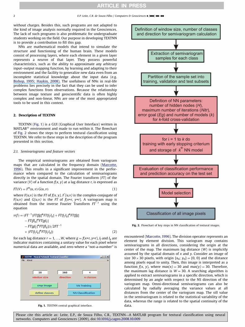
Fig. 2. Flowchart of key steps in NN classification of textural images.

2. Description of TEXTNN

TEXTNN (Fig. 1) is a GUI (Graphical User Interface) written inMATLABs environment and made to run within it. The flowchartof Fig. 2 shows the steps to perform textural classification usingTEXTNN. We refer to these steps in the description of the programpresented in this section.

2.1. Semivariograms and feature vectors

The empirical semivariograms are obtained from variogrammaps that are calculated in the frequency domain (Marcotte,1996). This results in a significant improvement in the perfor-mance when compared to the calculation of semivariogramsdirectly in the spatial domain. The Fourier transform (FT) of thevariance (V) of a function f(x, y) at a lag distance r, is expressed as

FTðVÞ ¼ Fnðu;vÞ Gðu;vÞ (1)

where F(u,v) is the FT of f(x, y), F*(u,v) is the complex-conjugate ofF(u,v) and G(u,v) is the FT of f(x+r, y+r). A variogram map isobtained from the inverse Fourier Transform FT�1 using theequation

vðf Þ ¼ ðFT�1fFT½fg�nFT½If Ig � þ FT½If Ig �

nFT½fg�

� FT½fIg �nFT½gIf �

� FT½gIf �nFT½fIg �gÞ=2FT�1

� fFT½If Ig �nFT½If Ig �g (2)

for each lag distance r ¼ 1,y, W, where g ¼ f(x+r, y+r), If and Ig areindicator matrices containing a unitary value for each pixel wherenumerical data are available, and zero where a ‘‘not-a-number’’ is

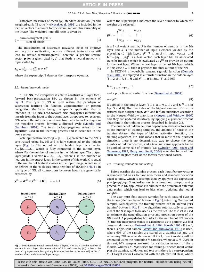
Fig. 1. TEXTNN central graphical interface.

Please cite this article as: Leite, E.P., de Souza Filho, C.R., TEXTNNnetworks. Computers and Geosciences (2009), doi:10.1016/j.cageo.2

encountered (Marcotte, 1996). The division operator represents anelement by element division. This variogram map containssemivariograms in all directions, considering the origin at thecenter of the map. The maximum lag distance (W) is implicitlyassumed by the spatial domain of x and y. Consider an image ofsize 30�30 pixels, with origin {x0; y0} ¼ {0, 0} and the distanceamong pixels equal to unity. Then, this image is interpreted as afunction f(x, y), where max(x) ¼ 30 and max(y) ¼ 30. Therefore,the maximum lag distance is W ¼ 30. A searching algorithm isapplied to extract semivariograms in a specific direction, which isdetermined by an angle with respect to the NS direction of thevariogram map. Omni-directional semivariograms can also becalculated by radially averaging the variance values at alldistances from the center of the variogram map. The sill valuein the semivariogram is related to the statistical variability of thedata, whereas the range is related to the spatial continuity of thedata.

—A MATLAB program for textural classification using neural008.10.009

ARTICLE IN PRESS

E.P. Leite, C.R. de Souza Filho / Computers & Geosciences ] (]]]]) ]]]–]]] 3

Histogram measures of mean (m), standard deviation (s) andweighted-rank fill ratio (Z) (Novak et al., 1993) are included in thefeature vectors to account for the overall radiometric variability ofthe image. The weighted-rank fill ratio is given by

Z ¼ sum k% brightest pixels

sum all pixels(3)

The introduction of histogram measures helps to improveaccuracy in classification, because different textures can stilllead to similar semivariograms. Therefore, a generic featurevector p for a given pixel (i, j) that feeds a neural network isrepresented by

pi;j ¼ ½g1i;j; . . . ; g

Wi;j ;m;s;Z�

T (4)

where the superscript T denotes the transpose operator.

2.2. Neural network model

In TEXTNN, the interpreter is able to construct a 3-layer feed-forward back-propagation NN, as shown in the scheme ofFig. 3. This type of NN is used within the paradigm ofsupervised learning for function approximation or patternrecognition, the latter being the specific application that isintended in TEXTNN. Feed-forward NNs propagates informationlinearly from the input to the output layer, as opposed to recurrentNNs where the information returns from later to earlier stages inthe modeling process, forming a directed cycle (Mandic andChambers, 2001). The term back-propagation refers to thealgorithm used in the learning process and is described in thenext section.

Each input feature vector p ¼ [p1,y, pP] presented to the NN isconstructed using Eq. (4) and is fully connected to the hiddenlayer (Fig. 3). The output of the hidden layer is a vectorh ¼ [h1,y, hH], which is fully connected to the output layer,where H is the number of neurons in the hidden layer. The outputlayer yields a vector o ¼ [o1,y, oC], where C is the number ofneurons in the output layer. In the context of this work, C is equalto the number of textural classes in the input image, which mustbe defined in the ‘n-classes’ input text box of TEXTNN (Fig. 1). Inthis type of NN, all connections between layers are genericallyexpressed by

yfLg ¼WfLg� xfL�1g þ bfLg; L ¼ 2;3 (5)

Fig. 3. Feed-forward neural network with 3 layers. P, H and C are the number of

neurons in each layer. Maximum value of P is W+3 (see Eq. (4)). H has to be

selected by experiment, but typically is a value that lies in the interval [10, 60]. C:

number of textural classes of input image.

Please cite this article as: Leite, E.P., de Souza Filho, C.R., TEXTNNnetworks. Computers and Geosciences (2009), doi:10.1016/j.cageo.20

where the superscript L indicates the layer number to which theweights are referred;

WfLg¼

w1;1 . . . w1;R

..

. . .. ..

.

wS;1 � � � wS;R

0BB@

1CCA (6)

is a S�R weight matrix; S is the number of neurons in the Lthlayer and R is the number of input elements yielded by thepreceding (L�1)th layer; y{L�1} is an R�1 input vector; andb{L}¼ [b1,y, bS]T is a bias vector. Each layer has an associated

transfer function which is evaluated at y{L} to provide an outputfor the next layer. When the next layer is the last NN layer, whichin this case L ¼ 3, then it provides the final output of the NN.

In TEXTNN, a hyperbolic tangent sigmoid function (Demuthet al., 2008) is employed as a transfer function in the hidden layer(L ¼ 2, R ¼ P, S ¼ H and x{1}

¼ p in Eqs. (5) and (6))

h ¼2

ð1þ e�2�yf2g Þ� 1 (7)

and a pure linear-transfer function (Demuth et al., 2008)

o ¼ yf3g (8)

is applied in the output layer (L ¼ 3, R ¼ H, S ¼ C and x{2}¼ h in

Eqs. 5 and 6). The row index of the highest element of o is thetextural class assigned to p. W{L} and b{L} are initialized accordingto the Nguyen–Widrow algorithm (Nguyen and Widrow, 1990)and they are updated iteratively by applying a gradient descentalgorithm in the training process described in Section 2.3.

The number of hidden neurons depends on several factors suchas the number of training samples, the amount of noise in thetraining dataset, the type of hidden activation function, thetraining algorithm, etc. This means that in most of the practicalsituations there is no deterministic way to choose the bestnumber of hidden neurons, and a trial and error approach has tobe applied. Some rule of thumbs (e.g. Swingler, 1996; Boger andGuterman, 1997; Berry and Linoff, 2004) may also be used, butsuch rules neglect most of the factors mentioned earlier.

2.3. Training, validation and testing

Before starting the training process, each input feature vector pis standardized so as to have zero mean and standard deviationequal to unity, which is accomplished by applying the expressionp0 ¼ (p�mP)/sP. Standardization is a common pre-processingprocedure in NN applications to eliminate the problem of differentdata scales, which can lead to bias when updating the neuralweights.

The user must first extract samples for each textural class inthe image (‘define classes’ button in Fig. 1), totalizing N-extractedsamples. Subsequently, the training process can be started (‘NNtraining’ button in Fig. 1): the algorithm automatically separates20% of the N samples to be used as the test set. The test set is usedto estimate the generalization error and prediction power of theNN model. A pop-up dialog box asks for the number of NN models(k) that the interpreter wants to calculate so as to perform a k-foldcross-validation (e.g. Plutowski et al., 1994; Hjorth, 1993). If k ¼ 1,then a single-split sample (Weiss and Kulikowski, 1991) is used,where 60% of the samples are stored as a training set and theremaining 20% as a validation set. If k41, then k models will begenerated using the remaining M samples, where M ¼ N�0.2N. Inthis set, M/k samples are used for validation in each of the k

models, whereas N�M/k is used for training. For each input vectorp in the training, validation and test sets, there is a correspondentC�1 target vector t associated with the jth textural class, where

—A MATLAB program for textural classification using neural08.10.009

ARTICLE IN PRESS

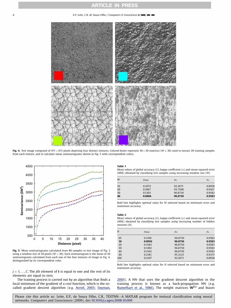
Fig. 4. Test image composed of 471�473 pixels depicting four distinct textures. Colored boxes represent 30�30 matrices (W ¼ 30) used to extract 20 training samples

from each texture, and to calculate mean semivariograms shown in Fig. 5 with correspondent colors.

0 5 10 15 20 25 30 35 40500

1000

1500

2000

2500

3000

3500

4000

4500

Distance (pixel)

Sem

ivar

ianc

e (D

N2 )

Fig. 5. Mean semivariograms calculated from 80 samples in test image of Fig. 2

using a window size of 30 pixels (W ¼ 30). Each semivariogram is the mean of 20

semivariograms calculated from each one of the four textures of image in Fig. 4,

distinguished by its correspondent color.

Table 1Mean values of global accuracy (G), kappa coefficient (k) and mean-squared error

(MSE) obtained by classifying test samples using increasing window size (W).

W mMSE mG mk

10 0.2072 92.1875 0.8958

20 0.1967 93.7500 0.9167

30 0.1303 96.8750 0.9583

40 0.0884 96.8750 0.9583

Bold line highlights optimal value for W selected based on minimum error and

maximum accuracy.

Table 2Mean values of global accuracy (G), kappa coefficient (k) and mean-squared error

(MSE) obtained by classifying test samples using increasing number of hidden

neurons (H).

H mMSE mG mk

05 0.1100 96.8750 0.9583

10 0.0956 96.8750 0.958320 0.1583 96.8750 0.9583

30 0.1492 96.8750 0.9583

40 0.1562 96.8750 0.9583

60 0.2181 95.3125 0.9375

100 0.2107 92.1875 0.8958

Bold line highlights optimal value for H selected based on minimum error and

maximum accuracy.

E.P. Leite, C.R. de Souza Filho / Computers & Geosciences ] (]]]]) ]]]–]]]4

j ¼ 1,y, C. The jth element of t is equal to one and the rest of itselements are equal to zero.

The training process is carried out by an algorithm that finds alocal minimum of the gradient of a cost function, which is the so-called gradient descent algorithm (e.g. Avriel, 2003; Snyman,

Please cite this article as: Leite, E.P., de Souza Filho, C.R., TEXTNNnetworks. Computers and Geosciences (2009), doi:10.1016/j.cageo.2

2005). A NN that uses the gradient descent algorithm in thetraining process is known as a back-propagation NN (e.g.Rumelhart et al., 1986). The weight matrices W{L} and biases

—A MATLAB program for textural classification using neural008.10.009

ARTICLE IN PRESS

Table 3Training error and performance results obtained using 6 combinations of features:

G ¼ global accuracy, k ¼ kappa coefficient and MSE ¼ mean-squared error.

p (i ¼ 1,y, 30) mMSE mG mk

[g(i)] H 0.38 93.75 0.92

[g(i), m] G 0.13 96.87 0.96

[g(i), s] F 0.11 96.87 0.96

[g(i), Z] E 0.40 85.94 0.81

[g(i), m, s] D 0.12 98.44 0.98

[c(i), l, g] C 0.09 100.00 1.00

[g(i), s, Z] B 0.14 96.87 0.96

[g(i), m, s, Z] A 0.15 96.87 0.96

Bold line highlights optimal combination of features selected based on minimum

error and maximum accuracy.

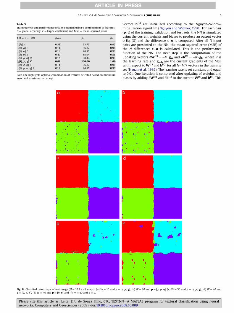
Fig. 6. Classified color maps of test image (H ¼ 10 for all maps): (a) W ¼ 10 and p ¼ [cp ¼ [c, l, g], (e) W ¼ 40 and p ¼ [c, g] and (f) W ¼ 40 and p ¼ c.

E.P. Leite, C.R. de Souza Filho / Computers & Geosciences ] (]]]]) ]]]–]]] 5

Please cite this article as: Leite, E.P., de Souza Filho, C.R., TEXTNNnetworks. Computers and Geosciences (2009), doi:10.1016/j.cageo.20

vectors b{L} are initialized according to the Nguyen–Widrowinitialization algorithm (Nguyen and Widrow, 1990). For each pair(p, t) of the training, validation and test sets, the NN is simulatedusing the current weights and biases to produce an output vectoro Eq. (8) and the difference t�o is computed. After all N inputpairs are presented to the NN, the mean-squared error (MSE) ofthe N differences t�o is calculated. This is the performancefunction of the NN. The next step is the computation of theupdating vectors dW{L}

¼ �lr � gw and db{L}¼ �lr �gb, where lr is

the learning rate and gw,b are the current gradients of the MSEwith respect to W{L} and b{L}, for all N�M/k vectors in the trainingset (Hagan et al., 1995). The learning rate is set constant and equalto 0.01. One iteration is completed after updating of weights andbiases by adding dW{L} and db{L} to the current W{L}and b{L}. This

, l, g], (b) W ¼ 20 and p ¼ [c, l, g], (c) W ¼ 30 and p ¼ [c, l, g], (d) W ¼ 40 and

—A MATLAB program for textural classification using neural08.10.009

ARTICLE IN PRESS

E.P. Leite, C.R. de Souza Filho / Computers & Geosciences ] (]]]]) ]]]–]]]6

process is carried out until one of the following conditions isachieved: (i) a minimization error goal (Eg) is reached in step (2),(ii) occurrence of three consecutive non-improvements in the MSEfor the validation set, which is called early-stopping or (iii) themaximum number of iterations (Nitr) is completed. Therefore,before the training process is started, the interpreter is requiredto enter the values of Nitr, H and Eg. The test set is used onlyto estimate the generalization error and the prediction power ofthe NN.

After the training process is completed, three confusionmatrices, for the Q (three) sets, are calculated and saved in a textfile. Confusion matrices constitute a very efficient and easy way toevaluate misclassification and are widely used in the realm ofpattern recognition. Each column of a confusion matrix representsthe frequencies of occurrences in the target classes, whereas eachrow represents the frequency of occurrences in the actual classes(Kohavi and Provost, 1998). The global accuracy GQ

¼P

i ¼ 1C sii

Q/NQ

and the kappa coefficient (Foody, 1992)

kQ ¼

NQ PCi¼1

sQii �

PCi¼1

siT sTi

ðNQÞ2�PCi¼1

siT sTi

(9)

are also calculated and stored in the same text file as theconfusion matrices. For each particular dataset Q, sii is the value inthe ith column and ith line of the respective confusion matrix. NQ

is the total number of samples, siT is the sum of the values in theith line and sTi is the sum of the values in the ith column. A plot ofG and k for the validation and test sets is automatically generatedafter the training process is completed. This provides enoughquantitative information for the interpreter about how thedesigned NN is performing on known and unknown data.

2.4. Model selection and generalization

The k models calculated in the training process are stored sothat the interpreter can select the best model by comparing theconfusion matrices, MSEs, global accuracies and kappa coeffi-cients amongst them. After model selection, the classification ofall image pixels (generalization) can be performed using the ‘NNclassify’ button (Fig. 1), where the user must provide the numberassociated with the selected NN model. The output is a coloredclassified map. Subsequently, the interpreter may also return tothe ‘NN classify’ button and select another one of the k models tovisually compare the mapped features in the classified images.

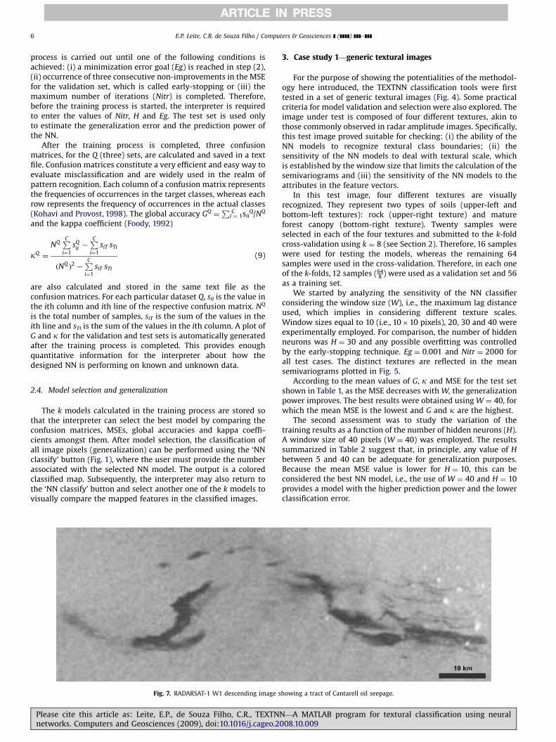
Fig. 7. RADARSAT-1 W1 descending image s

Please cite this article as: Leite, E.P., de Souza Filho, C.R., TEXTNNnetworks. Computers and Geosciences (2009), doi:10.1016/j.cageo.2

3. Case study 1—generic textural images

For the purpose of showing the potentialities of the methodol-ogy here introduced, the TEXTNN classification tools were firsttested in a set of generic textural images (Fig. 4). Some practicalcriteria for model validation and selection were also explored. Theimage under test is composed of four different textures, akin tothose commonly observed in radar amplitude images. Specifically,this test image proved suitable for checking: (i) the ability of theNN models to recognize textural class boundaries; (ii) thesensitivity of the NN models to deal with textural scale, whichis established by the window size that limits the calculation of thesemivariograms and (iii) the sensitivity of the NN models to theattributes in the feature vectors.

In this test image, four different textures are visuallyrecognized. They represent two types of soils (upper-left andbottom-left textures): rock (upper-right texture) and matureforest canopy (bottom-right texture). Twenty samples wereselected in each of the four textures and submitted to the k-foldcross-validation using k ¼ 8 (see Section 2). Therefore, 16 sampleswere used for testing the models, whereas the remaining 64samples were used in the cross-validation. Therefore, in each oneof the k-folds, 12 samples (64

8 ) were used as a validation set and 56as a training set.

We started by analyzing the sensitivity of the NN classifierconsidering the window size (W), i.e., the maximum lag distanceused, which implies in considering different texture scales.Window sizes equal to 10 (i.e., 10�10 pixels), 20, 30 and 40 wereexperimentally employed. For comparison, the number of hiddenneurons was H ¼ 30 and any possible overfitting was controlledby the early-stopping technique. Eg ¼ 0.001 and Nitr ¼ 2000 forall test cases. The distinct textures are reflected in the meansemivariograms plotted in Fig. 5.

According to the mean values of G, k and MSE for the test setshown in Table 1, as the MSE decreases with W, the generalizationpower improves. The best results were obtained using W ¼ 40, forwhich the mean MSE is the lowest and G and k are the highest.

The second assessment was to study the variation of thetraining results as a function of the number of hidden neurons (H).A window size of 40 pixels (W ¼ 40) was employed. The resultssummarized in Table 2 suggest that, in principle, any value of H

between 5 and 40 can be adequate for generalization purposes.Because the mean MSE value is lower for H ¼ 10, this can beconsidered the best NN model, i.e., the use of W ¼ 40 and H ¼ 10provides a model with the higher prediction power and the lowerclassification error.

howing a tract of Cantarell oil seepage.

—A MATLAB program for textural classification using neural008.10.009

ARTICLE IN PRESS

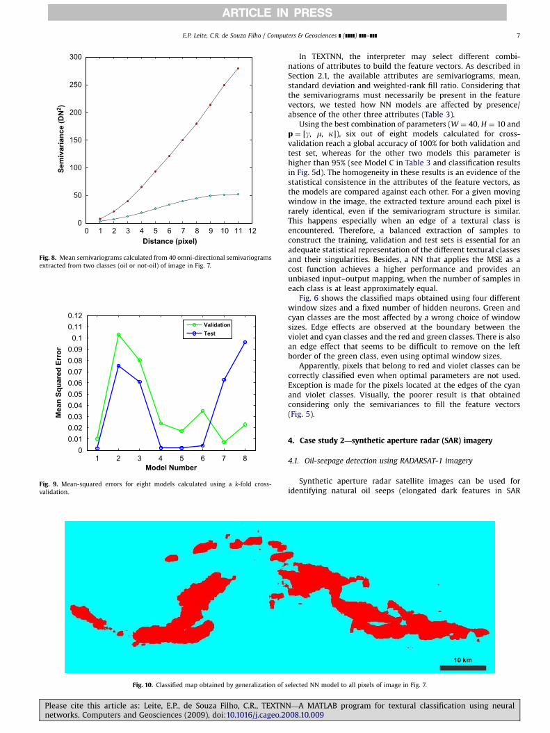
Fig. 10. Classified map obtained by generalization of s

0 1 2 3 4 5 6 7 8 9 10 11 120

50

100

150

200

250

300

Distance (pixel)

Sem

ivar

ianc

e (D

N2 )

Fig. 8. Mean semivariograms calculated from 40 omni-directional semivariograms

extracted from two classes (oil or not-oil) of image in Fig. 7.

1 2 3 4 5 6 7 80

0.010.020.030.040.050.060.070.080.090.10.110.12

Model Number

Mea

n Sq

uare

d Er

ror

ValidationTest

Fig. 9. Mean-squared errors for eight models calculated using a k-fold cross-

validation.

E.P. Leite, C.R. de Souza Filho / Computers & Geosciences ] (]]]]) ]]]–]]] 7

Please cite this article as: Leite, E.P., de Souza Filho, C.R., TEXTNNnetworks. Computers and Geosciences (2009), doi:10.1016/j.cageo.20

In TEXTNN, the interpreter may select different combi-nations of attributes to build the feature vectors. As described inSection 2.1, the available attributes are semivariograms, mean,standard deviation and weighted-rank fill ratio. Considering thatthe semivariograms must necessarily be present in the featurevectors, we tested how NN models are affected by presence/absence of the other three attributes (Table 3).

Using the best combination of parameters (W ¼ 40, H ¼ 10 andp ¼ [g, m, k]), six out of eight models calculated for cross-validation reach a global accuracy of 100% for both validation andtest set, whereas for the other two models this parameter ishigher than 95% (see Model C in Table 3 and classification resultsin Fig. 5d). The homogeneity in these results is an evidence of thestatistical consistence in the attributes of the feature vectors, asthe models are compared against each other. For a given movingwindow in the image, the extracted texture around each pixel israrely identical, even if the semivariogram structure is similar.This happens especially when an edge of a textural class isencountered. Therefore, a balanced extraction of samples toconstruct the training, validation and test sets is essential for anadequate statistical representation of the different textural classesand their singularities. Besides, a NN that applies the MSE as acost function achieves a higher performance and provides anunbiased input–output mapping, when the number of samples ineach class is at least approximately equal.

Fig. 6 shows the classified maps obtained using four differentwindow sizes and a fixed number of hidden neurons. Green andcyan classes are the most affected by a wrong choice of windowsizes. Edge effects are observed at the boundary between theviolet and cyan classes and the red and green classes. There is alsoan edge effect that seems to be difficult to remove on the leftborder of the green class, even using optimal window sizes.

Apparently, pixels that belong to red and violet classes can becorrectly classified even when optimal parameters are not used.Exception is made for the pixels located at the edges of the cyanand violet classes. Visually, the poorer result is that obtainedconsidering only the semivariances to fill the feature vectors(Fig. 5).

4. Case study 2—synthetic aperture radar (SAR) imagery

4.1. Oil-seepage detection using RADARSAT-1 imagery

Synthetic aperture radar satellite images can be used foridentifying natural oil seeps (elongated dark features in SAR

elected NN model to all pixels of image in Fig. 7.

—A MATLAB program for textural classification using neural08.10.009

ARTICLE IN PRESS

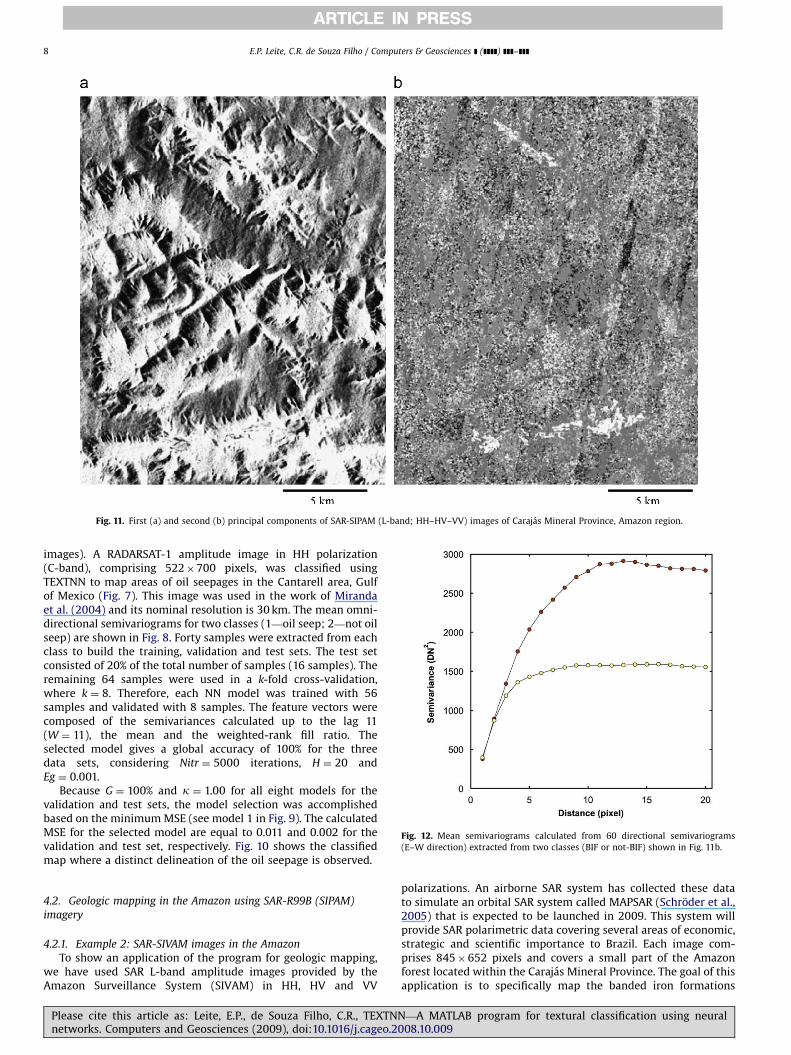
Fig. 12. Mean semivariograms calculated from 60 directional semivariograms

(E–W direction) extracted from two classes (BIF or not-BIF) shown in Fig. 11b.

Fig. 11. First (a) and second (b) principal components of SAR-SIPAM (L-band; HH–HV–VV) images of Carajas Mineral Province, Amazon region.

E.P. Leite, C.R. de Souza Filho / Computers & Geosciences ] (]]]]) ]]]–]]]8

images). A RADARSAT-1 amplitude image in HH polarization(C-band), comprising 522�700 pixels, was classified usingTEXTNN to map areas of oil seepages in the Cantarell area, Gulfof Mexico (Fig. 7). This image was used in the work of Mirandaet al. (2004) and its nominal resolution is 30 km. The mean omni-directional semivariograms for two classes (1—oil seep; 2—not oilseep) are shown in Fig. 8. Forty samples were extracted from eachclass to build the training, validation and test sets. The test setconsisted of 20% of the total number of samples (16 samples). Theremaining 64 samples were used in a k-fold cross-validation,where k ¼ 8. Therefore, each NN model was trained with 56samples and validated with 8 samples. The feature vectors werecomposed of the semivariances calculated up to the lag 11(W ¼ 11), the mean and the weighted-rank fill ratio. Theselected model gives a global accuracy of 100% for the threedata sets, considering Nitr ¼ 5000 iterations, H ¼ 20 andEg ¼ 0.001.

Because G ¼ 100% and k ¼ 1.00 for all eight models for thevalidation and test sets, the model selection was accomplishedbased on the minimum MSE (see model 1 in Fig. 9). The calculatedMSE for the selected model are equal to 0.011 and 0.002 for thevalidation and test set, respectively. Fig. 10 shows the classifiedmap where a distinct delineation of the oil seepage is observed.

4.2. Geologic mapping in the Amazon using SAR-R99B (SIPAM)

imagery

4.2.1. Example 2: SAR-SIVAM images in the Amazon

To show an application of the program for geologic mapping,we have used SAR L-band amplitude images provided by theAmazon Surveillance System (SIVAM) in HH, HV and VV

Please cite this article as: Leite, E.P., de Souza Filho, C.R., TEXTNNnetworks. Computers and Geosciences (2009), doi:10.1016/j.cageo.2

polarizations. An airborne SAR system has collected these datato simulate an orbital SAR system called MAPSAR (Schroder et al.,2005) that is expected to be launched in 2009. This system willprovide SAR polarimetric data covering several areas of economic,strategic and scientific importance to Brazil. Each image com-prises 845�652 pixels and covers a small part of the Amazonforest located within the Carajas Mineral Province. The goal of thisapplication is to specifically map the banded iron formations

—A MATLAB program for textural classification using neural008.10.009

ARTICLE IN PRESS

E.P. Leite, C.R. de Souza Filho / Computers & Geosciences ] (]]]]) ]]]–]]] 9

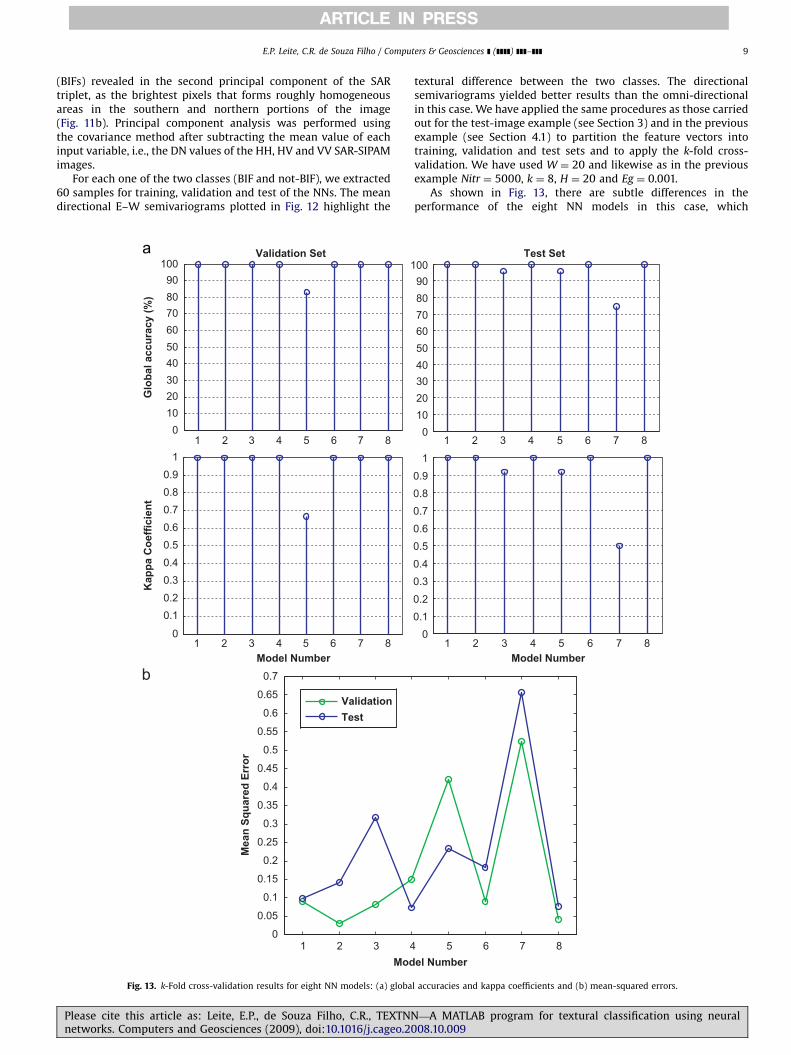
(BIFs) revealed in the second principal component of the SARtriplet, as the brightest pixels that forms roughly homogeneousareas in the southern and northern portions of the image(Fig. 11b). Principal component analysis was performed usingthe covariance method after subtracting the mean value of eachinput variable, i.e., the DN values of the HH, HV and VV SAR-SIPAMimages.

For each one of the two classes (BIF and not-BIF), we extracted60 samples for training, validation and test of the NNs. The meandirectional E–W semivariograms plotted in Fig. 12 highlight the

1 2 3 4 5 6 7 80102030405060708090100

Glo

bal a

ccur

acy

(%)

Validation Set

1 2 3 4 5 6 7 80

0.10.20.30.40.50.60.70.80.91

Kap

pa C

oeffi

cien

t

Model Number

1

1 2 3 40

0.05

0.1

0.15

0.2

0.25

0.3

0.35

0.4

0.45

0.5

0.55

0.6

0.65

0.7

Mod

Mea

n Sq

uare

d Er

ror

ValidationTest

Fig. 13. k-Fold cross-validation results for eight NN models: (a) globa

Please cite this article as: Leite, E.P., de Souza Filho, C.R., TEXTNNnetworks. Computers and Geosciences (2009), doi:10.1016/j.cageo.20

textural difference between the two classes. The directionalsemivariograms yielded better results than the omni-directionalin this case. We have applied the same procedures as those carriedout for the test-image example (see Section 3) and in the previousexample (see Section 4.1) to partition the feature vectors intotraining, validation and test sets and to apply the k-fold cross-validation. We have used W ¼ 20 and likewise as in the previousexample Nitr ¼ 5000, k ¼ 8, H ¼ 20 and Eg ¼ 0.001.

As shown in Fig. 13, there are subtle differences in theperformance of the eight NN models in this case, which

1 2 3 4 5 6 7 8010203040506070809000

Test Set

1 2 3 4 5 6 7 80

0.10.20.30.40.50.60.70.80.91

Model Number

5 6 7 8el Number

l accuracies and kappa coefficients and (b) mean-squared errors.

—A MATLAB program for textural classification using neural08.10.009

ARTICLE IN PRESS

5 km

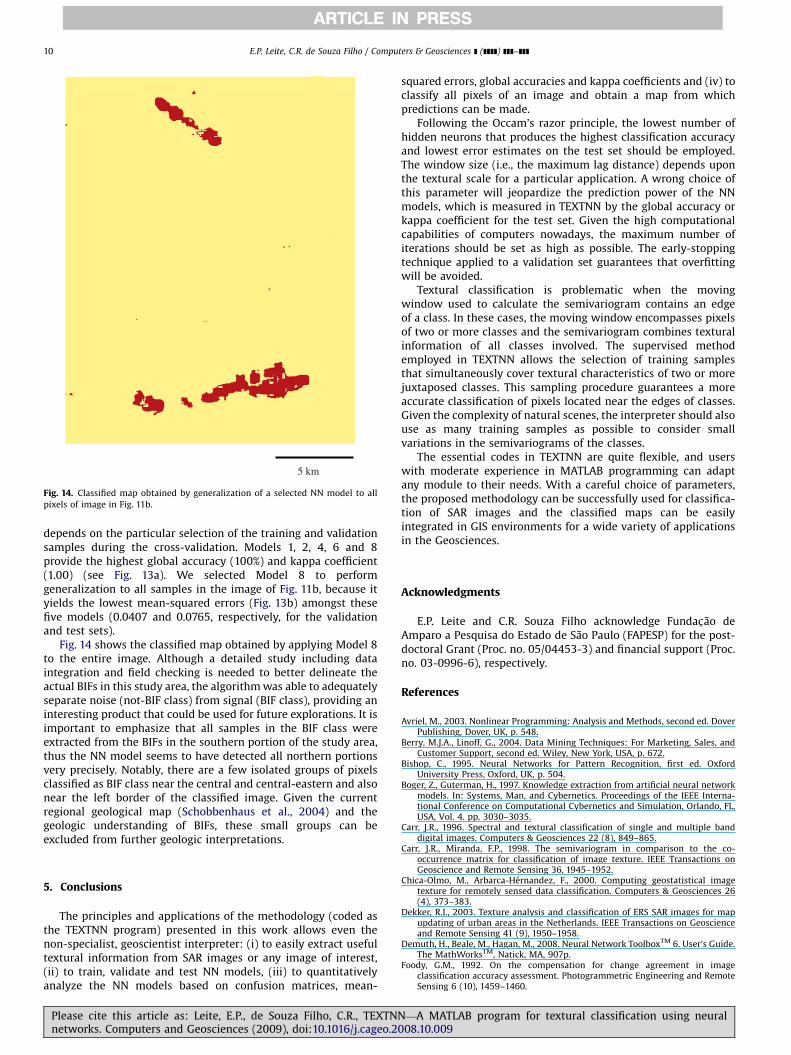
Fig. 14. Classified map obtained by generalization of a selected NN model to all

pixels of image in Fig. 11b.

E.P. Leite, C.R. de Souza Filho / Computers & Geosciences ] (]]]]) ]]]–]]]10

depends on the particular selection of the training and validationsamples during the cross-validation. Models 1, 2, 4, 6 and 8provide the highest global accuracy (100%) and kappa coefficient(1.00) (see Fig. 13a). We selected Model 8 to performgeneralization to all samples in the image of Fig. 11b, because ityields the lowest mean-squared errors (Fig. 13b) amongst thesefive models (0.0407 and 0.0765, respectively, for the validationand test sets).

Fig. 14 shows the classified map obtained by applying Model 8to the entire image. Although a detailed study including dataintegration and field checking is needed to better delineate theactual BIFs in this study area, the algorithm was able to adequatelyseparate noise (not-BIF class) from signal (BIF class), providing aninteresting product that could be used for future explorations. It isimportant to emphasize that all samples in the BIF class wereextracted from the BIFs in the southern portion of the study area,thus the NN model seems to have detected all northern portionsvery precisely. Notably, there are a few isolated groups of pixelsclassified as BIF class near the central and central-eastern and alsonear the left border of the classified image. Given the currentregional geological map (Schobbenhaus et al., 2004) and thegeologic understanding of BIFs, these small groups can beexcluded from further geologic interpretations.

5. Conclusions

The principles and applications of the methodology (coded asthe TEXTNN program) presented in this work allows even thenon-specialist, geoscientist interpreter: (i) to easily extract usefultextural information from SAR images or any image of interest,(ii) to train, validate and test NN models, (iii) to quantitativelyanalyze the NN models based on confusion matrices, mean-

Please cite this article as: Leite, E.P., de Souza Filho, C.R., TEXTNNnetworks. Computers and Geosciences (2009), doi:10.1016/j.cageo.2

squared errors, global accuracies and kappa coefficients and (iv) toclassify all pixels of an image and obtain a map from whichpredictions can be made.

Following the Occam’s razor principle, the lowest number ofhidden neurons that produces the highest classification accuracyand lowest error estimates on the test set should be employed.The window size (i.e., the maximum lag distance) depends uponthe textural scale for a particular application. A wrong choice ofthis parameter will jeopardize the prediction power of the NNmodels, which is measured in TEXTNN by the global accuracy orkappa coefficient for the test set. Given the high computationalcapabilities of computers nowadays, the maximum number ofiterations should be set as high as possible. The early-stoppingtechnique applied to a validation set guarantees that overfittingwill be avoided.

Textural classification is problematic when the movingwindow used to calculate the semivariogram contains an edgeof a class. In these cases, the moving window encompasses pixelsof two or more classes and the semivariogram combines texturalinformation of all classes involved. The supervised methodemployed in TEXTNN allows the selection of training samplesthat simultaneously cover textural characteristics of two or morejuxtaposed classes. This sampling procedure guarantees a moreaccurate classification of pixels located near the edges of classes.Given the complexity of natural scenes, the interpreter should alsouse as many training samples as possible to consider smallvariations in the semivariograms of the classes.

The essential codes in TEXTNN are quite flexible, and userswith moderate experience in MATLAB programming can adaptany module to their needs. With a careful choice of parameters,the proposed methodology can be successfully used for classifica-tion of SAR images and the classified maps can be easilyintegrated in GIS environments for a wide variety of applicationsin the Geosciences.

Acknowledgments

E.P. Leite and C.R. Souza Filho acknowledge Fundac- ao deAmparo a Pesquisa do Estado de Sao Paulo (FAPESP) for the post-doctoral Grant (Proc. no. 05/04453-3) and financial support (Proc.no. 03-0996-6), respectively.

References

Avriel, M., 2003. Nonlinear Programming: Analysis and Methods, second ed. DoverPublishing, Dover, UK, p. 548.

Berry, M.J.A., Linoff, G., 2004. Data Mining Techniques: For Marketing, Sales, andCustomer Support, second ed. Wiley, New York, USA, p. 672.

Bishop, C., 1995. Neural Networks for Pattern Recognition, first ed. OxfordUniversity Press, Oxford, UK, p. 504.

Boger, Z., Guterman, H., 1997. Knowledge extraction from artificial neural networkmodels. In: Systems, Man, and Cybernetics. Proceedings of the IEEE Interna-tional Conference on Computational Cybernetics and Simulation, Orlando, FL,USA, Vol. 4. pp. 3030–3035.

Carr, J.R., 1996. Spectral and textural classification of single and multiple banddigital images. Computers & Geosciences 22 (8), 849–865.

Carr, J.R., Miranda, F.P., 1998. The semivariogram in comparison to the co-occurrence matrix for classification of image texture. IEEE Transactions onGeoscience and Remote Sensing 36, 1945–1952.

Chica-Olmo, M., Arbarca-Hernandez, F., 2000. Computing geostatistical imagetexture for remotely sensed data classification. Computers & Geosciences 26(4), 373–383.

Dekker, R.J., 2003. Texture analysis and classification of ERS SAR images for mapupdating of urban areas in the Netherlands. IEEE Transactions on Geoscienceand Remote Sensing 41 (9), 1950–1958.

Demuth, H., Beale, M., Hagan, M., 2008. Neural Network ToolboxTM 6. User’s Guide.The MathWorksTM, Natick, MA, 907p.

Foody, G.M., 1992. On the compensation for change agreement in imageclassification accuracy assessment. Photogrammetric Engineering and RemoteSensing 6 (10), 1459–1460.

—A MATLAB program for textural classification using neural008.10.009

ARTICLE IN PRESS

E.P. Leite, C.R. de Souza Filho / Computers & Geosciences ] (]]]]) ]]]–]]] 11

Gao, D., 2004. Texture model regression for effective feature discrimination:application to seismic facies visualization and interpretation. Geophysics 69,958–967.

Gao, D., 2008. Application of seismic texture model regression to seismic faciescharacterization and interpretation. The Leading Edge 27, 394–397.

Hagan, M.T., Demuth, H.B., Beale, M.H., 1995. Neural Network Design, first ed. PWSPublishing, Boston, MA, USA, p. 736.

Haykin, S., 2008. Neural Networks: A Comprehensive Foundation, third ed. PrenticeHall, Upper Saddle River, NJ, USA, p. 906.

Hjorth, J.S.U., 1993. Computer Intensive Statistical Methods Validation, ModelSelection, and Bootstrap, first ed. Chapman & Hall, London, UK, p. 263.

Kohavi, R., Provost, F., 1998. Glossary of terms: editorial for the special issue onapplications of machine learning and the knowledge discovery process.Machine Learning 30, 217–274.

Kurosu, T., Yokoyama, S., Fujita, M., Chiba, K., 2001. Land-use classification withtextural analysis and the aggregation technique using multi-temporal JERS-1L-band SAR images. International Journal of Remote Sensing 22 (4), 595–613.

Li, P., Li, Z., Moon, W.M., 2001. Lithological discrimination of Altun area innorthwest China using Landsat TM data and geostatistical textural informa-tion. Geosciences Journal 5 (4), 293–300.

Mandic, D.P., Chambers, J.A., 2001. Recurrent Neural Networks for Prediction:Learning Algorithms, Architectures and Stability, first ed. Wiley, Chichester, UK,p. 306.

Marcotte, D., 1996. Fast variogram computation with FFT. Computers & Geo-sciences 22 (10), 1175–1186.

Marmo, R., Amodio, S., Tagliaferri, R., Ferreri, V., Longo, G., 2005. Texturalidentification of carbonate rocks by image processing and neural network:methodology proposal and examples. Computers & Geosciences 31 (5),649–659.

Miranda, F.P., Fonseca, L.E.N., Carr, J.R., 1998. Semivariogram textural classificationof JERS-1 (Fuyo-1) SAR data obtained over a flooded area of the Amazonrainforest. International Journal of Remote Sensing 19, 549–556.

Miranda, F.P., Marmol, A.M.Q., Pedroso, E.C., Beisl, C.H., Welgan, P., Morales, L.M.,2004. Analysis of RADARSAT-1 data for offshore monitoring activities in theCantarell Complex, Gulf of Mexico, using the unsupervised semivariogramtextural classifier (USTC). Canadian Journal of Remote Sensing 30 (3), 424–436.

Please cite this article as: Leite, E.P., de Souza Filho, C.R., TEXTNNnetworks. Computers and Geosciences (2009), doi:10.1016/j.cageo.20

Moysey, S., Knight, R.J., Jol, H.M., 2006. Texture-based classification of ground-penetrating radar images. Geophysics 71 (6), K111–K118.

Novak, L.M., Owirka, G.J., Netishen, C.M., 1993. Performance of a high-resolutionpolarimetric SAR automatic target recognition system. The Lincoln LaboratoryJournal 6 (1), 11–23.

Nguyen, D., Widrow. B., 1990. Improving the learning speed of 2-layer neuralnetworks by choosing initial values of the adaptive weights. In: Proceedings ofthe International Joint Conference on Neural Networks 3, Washington, DC,USA, pp. 21–26.

Plutowski, M., Sakata, S., White, H., 1994. Cross-validation estimates IMSE. In:Cowan, J.D., Tesauro, G., Alspector, J. (Eds.), Advances in Neural Informa-tion Processing Systems 6. Morgan Kaufman, San Mateo, CA, USA,pp. 391–398.

Rumelhart, D.E., Hinton, G.E., Williams, R.J., 1986. Learning internal represen-tations by error propagation. In: Rumelhart, D.E., Mclelland, J.L. (Eds.),Parallel Distributed Processing 1. MIT Press, Cambridge, MA, USA,pp. 318–362.

Schobbenhaus, C., Gonc-alves, J.H., Santos, J.O.S., Abram, M.B., Leao Neto, R., Matos,G.M.M., Vidotti, R.M., Ramos, M.A.B., Jesus, J.D.A., 2004. Geological chart ofBrazil 1:1 Million GIS. In: Proceedings of the 32nd International GeologicalCongress, 2004, Florence, Italy.

Schroder, R., Puls, J., Hanjnsek, I., Jochim, F., Neff, T., Kono, J., Paradella, W.R., Silva,M.M.Q., Valeriano, D.M., Maycira, P.F.C., 2005. MAPSAR: a small L-band SARmission for land observation. Acta Astronautica 56, 35–43.

Snyman, J., 2005. Practical Mathematical Optimization: An Introduction to BasicOptimization Theory and Classical and New Gradient-Based Algorithms, firsted. Springer Publishing, New York, USA, p. 257.

Swingler, K., 1996. Applying Neural Networks: A Practical Guide, first ed. MorganKaufmann Publishers, Inc., San Francisco, CA, USA, p. 303.

Tercier, P., Knight, R.J., Jol, H.M., 2000. A comparison of the correlation structure inGPR images of deltaic and barrier-spit depositional environments. Geophysics65, 1142–1153.

Weiss, S.M., Kulikowski, C.A., 1991. Computer Systems That Learn: Classificationand Prediction Methods from Statistics, Neural Nets, Machine Learning, andExpert Systems, first ed. Morgan Kaufmann Publishers, San Francisco, CA, USA,p. 223.

—A MATLAB program for textural classification using neural08.10.009