Embed Size (px)
Citation preview

TGCC public DocumentationRelease 2022-07-18.1712
CEA
2022-07-18

CONTENT
1 Introduction 11.1 The computing center . . . . . . . . . . . . . . . . . . . . . . . . . . . . . . . . . . . . . . . . . . 11.2 Access to computing resources . . . . . . . . . . . . . . . . . . . . . . . . . . . . . . . . . . . . . . 2
2 Supercomputer architecture 32.1 Configuration of Irene . . . . . . . . . . . . . . . . . . . . . . . . . . . . . . . . . . . . . . . . . . 32.2 Interconnect . . . . . . . . . . . . . . . . . . . . . . . . . . . . . . . . . . . . . . . . . . . . . . . 62.3 Lustre . . . . . . . . . . . . . . . . . . . . . . . . . . . . . . . . . . . . . . . . . . . . . . . . . . . 6
3 User account 9
4 Interactive access 114.1 System access . . . . . . . . . . . . . . . . . . . . . . . . . . . . . . . . . . . . . . . . . . . . . . 114.2 Login nodes usage . . . . . . . . . . . . . . . . . . . . . . . . . . . . . . . . . . . . . . . . . . . . 11
5 Data spaces 155.1 Available file systems . . . . . . . . . . . . . . . . . . . . . . . . . . . . . . . . . . . . . . . . . . 155.2 Quota . . . . . . . . . . . . . . . . . . . . . . . . . . . . . . . . . . . . . . . . . . . . . . . . . . . 185.3 Data protection . . . . . . . . . . . . . . . . . . . . . . . . . . . . . . . . . . . . . . . . . . . . . . 205.4 Personal Spaces . . . . . . . . . . . . . . . . . . . . . . . . . . . . . . . . . . . . . . . . . . . . . 205.5 Shared Spaces . . . . . . . . . . . . . . . . . . . . . . . . . . . . . . . . . . . . . . . . . . . . . . 205.6 Parallel file system usage monitoring . . . . . . . . . . . . . . . . . . . . . . . . . . . . . . . . . . 27
6 Data transfers 296.1 File transfer . . . . . . . . . . . . . . . . . . . . . . . . . . . . . . . . . . . . . . . . . . . . . . . . 296.2 CCFR infrastructure . . . . . . . . . . . . . . . . . . . . . . . . . . . . . . . . . . . . . . . . . . . 316.3 PRACE infrastructure . . . . . . . . . . . . . . . . . . . . . . . . . . . . . . . . . . . . . . . . . . 31
7 Environment management 337.1 What is module . . . . . . . . . . . . . . . . . . . . . . . . . . . . . . . . . . . . . . . . . . . . . . 337.2 Module actions . . . . . . . . . . . . . . . . . . . . . . . . . . . . . . . . . . . . . . . . . . . . . . 337.3 Initialization and scope . . . . . . . . . . . . . . . . . . . . . . . . . . . . . . . . . . . . . . . . . . 357.4 Major modulefiles . . . . . . . . . . . . . . . . . . . . . . . . . . . . . . . . . . . . . . . . . . . . 367.5 Extend your environment with modulefiles . . . . . . . . . . . . . . . . . . . . . . . . . . . . . . . 40
8 Softwares 458.1 Generalities on software . . . . . . . . . . . . . . . . . . . . . . . . . . . . . . . . . . . . . . . . . 458.2 Specific software . . . . . . . . . . . . . . . . . . . . . . . . . . . . . . . . . . . . . . . . . . . . . 478.3 Product Life cycle . . . . . . . . . . . . . . . . . . . . . . . . . . . . . . . . . . . . . . . . . . . . 48
9 Job submission 51
i
9.1 Scheduling policy . . . . . . . . . . . . . . . . . . . . . . . . . . . . . . . . . . . . . . . . . . . . 519.2 Choosing the file systems . . . . . . . . . . . . . . . . . . . . . . . . . . . . . . . . . . . . . . . . 529.3 Submission scripts . . . . . . . . . . . . . . . . . . . . . . . . . . . . . . . . . . . . . . . . . . . . 529.4 Job monitoring and control . . . . . . . . . . . . . . . . . . . . . . . . . . . . . . . . . . . . . . . . 599.5 Special jobs . . . . . . . . . . . . . . . . . . . . . . . . . . . . . . . . . . . . . . . . . . . . . . . . 68
10 Project accounting 7310.1 Computing hours consumption control process . . . . . . . . . . . . . . . . . . . . . . . . . . . . . 7310.2 ccc_myproject . . . . . . . . . . . . . . . . . . . . . . . . . . . . . . . . . . . . . . . . . . . . . . 7410.3 ccc_compuse . . . . . . . . . . . . . . . . . . . . . . . . . . . . . . . . . . . . . . . . . . . . . . . 75
11 Compilation 7711.1 Language standard . . . . . . . . . . . . . . . . . . . . . . . . . . . . . . . . . . . . . . . . . . . . 7711.2 Available compilers . . . . . . . . . . . . . . . . . . . . . . . . . . . . . . . . . . . . . . . . . . . 7711.3 Available numerical libraries . . . . . . . . . . . . . . . . . . . . . . . . . . . . . . . . . . . . . . . 8211.4 Compiling for Skylake . . . . . . . . . . . . . . . . . . . . . . . . . . . . . . . . . . . . . . . . . . 8311.5 Compiling for Rome/Milan . . . . . . . . . . . . . . . . . . . . . . . . . . . . . . . . . . . . . . . 83
12 Parallel programming 8512.1 MPI . . . . . . . . . . . . . . . . . . . . . . . . . . . . . . . . . . . . . . . . . . . . . . . . . . . . 8512.2 OpenMP . . . . . . . . . . . . . . . . . . . . . . . . . . . . . . . . . . . . . . . . . . . . . . . . . 9012.3 Using GPUs . . . . . . . . . . . . . . . . . . . . . . . . . . . . . . . . . . . . . . . . . . . . . . . 90
13 Runtime tuning 9313.1 Memory allocation tuning . . . . . . . . . . . . . . . . . . . . . . . . . . . . . . . . . . . . . . . . 93
14 Process distribution, affinity and binding 9514.1 Hardware topology . . . . . . . . . . . . . . . . . . . . . . . . . . . . . . . . . . . . . . . . . . . . 9514.2 Definitions . . . . . . . . . . . . . . . . . . . . . . . . . . . . . . . . . . . . . . . . . . . . . . . . 9514.3 Process distribution . . . . . . . . . . . . . . . . . . . . . . . . . . . . . . . . . . . . . . . . . . . 9514.4 Process and thread affinity . . . . . . . . . . . . . . . . . . . . . . . . . . . . . . . . . . . . . . . . 10014.5 Hyper-Threading usage . . . . . . . . . . . . . . . . . . . . . . . . . . . . . . . . . . . . . . . . . . 10214.6 Turbo . . . . . . . . . . . . . . . . . . . . . . . . . . . . . . . . . . . . . . . . . . . . . . . . . . . 103
15 Parallel IO 10515.1 MPI-IO . . . . . . . . . . . . . . . . . . . . . . . . . . . . . . . . . . . . . . . . . . . . . . . . . . 10515.2 Recommended data usage on parallel file system . . . . . . . . . . . . . . . . . . . . . . . . . . . . 10515.3 Parallel compression and decompression with pigz . . . . . . . . . . . . . . . . . . . . . . . . . . . 107
16 Debugging 10916.1 Summary . . . . . . . . . . . . . . . . . . . . . . . . . . . . . . . . . . . . . . . . . . . . . . . . . 10916.2 Compiler flags . . . . . . . . . . . . . . . . . . . . . . . . . . . . . . . . . . . . . . . . . . . . . . 10916.3 Available debuggers . . . . . . . . . . . . . . . . . . . . . . . . . . . . . . . . . . . . . . . . . . . 11016.4 Other tools . . . . . . . . . . . . . . . . . . . . . . . . . . . . . . . . . . . . . . . . . . . . . . . . 117
17 Profiling 12517.1 Summary . . . . . . . . . . . . . . . . . . . . . . . . . . . . . . . . . . . . . . . . . . . . . . . . . 12517.2 IPM . . . . . . . . . . . . . . . . . . . . . . . . . . . . . . . . . . . . . . . . . . . . . . . . . . . . 12717.3 Darshan . . . . . . . . . . . . . . . . . . . . . . . . . . . . . . . . . . . . . . . . . . . . . . . . . . 12817.4 Arm-forge MAP . . . . . . . . . . . . . . . . . . . . . . . . . . . . . . . . . . . . . . . . . . . . . 13017.5 Gprof . . . . . . . . . . . . . . . . . . . . . . . . . . . . . . . . . . . . . . . . . . . . . . . . . . . 13117.6 igprof . . . . . . . . . . . . . . . . . . . . . . . . . . . . . . . . . . . . . . . . . . . . . . . . . . . 13217.7 PAPI . . . . . . . . . . . . . . . . . . . . . . . . . . . . . . . . . . . . . . . . . . . . . . . . . . . 13317.8 Scalasca . . . . . . . . . . . . . . . . . . . . . . . . . . . . . . . . . . . . . . . . . . . . . . . . . 13617.9 Vampir . . . . . . . . . . . . . . . . . . . . . . . . . . . . . . . . . . . . . . . . . . . . . . . . . . 140
ii
17.10 Extra-P . . . . . . . . . . . . . . . . . . . . . . . . . . . . . . . . . . . . . . . . . . . . . . . . . . 14117.11 HPCToolkit . . . . . . . . . . . . . . . . . . . . . . . . . . . . . . . . . . . . . . . . . . . . . . . . 14617.12 Intel Vtune . . . . . . . . . . . . . . . . . . . . . . . . . . . . . . . . . . . . . . . . . . . . . . . . 14917.13 Valgrind . . . . . . . . . . . . . . . . . . . . . . . . . . . . . . . . . . . . . . . . . . . . . . . . . 15417.14 Intel Advisor . . . . . . . . . . . . . . . . . . . . . . . . . . . . . . . . . . . . . . . . . . . . . . . 15617.15 TAU (Tuning and Analysis Utilities) . . . . . . . . . . . . . . . . . . . . . . . . . . . . . . . . . . . 15717.16 Gprof2dot . . . . . . . . . . . . . . . . . . . . . . . . . . . . . . . . . . . . . . . . . . . . . . . . 16217.17 Perf . . . . . . . . . . . . . . . . . . . . . . . . . . . . . . . . . . . . . . . . . . . . . . . . . . . . 16317.18 Memonit . . . . . . . . . . . . . . . . . . . . . . . . . . . . . . . . . . . . . . . . . . . . . . . . . 165
18 Post-processing 16718.1 Gnuplot . . . . . . . . . . . . . . . . . . . . . . . . . . . . . . . . . . . . . . . . . . . . . . . . . . 16718.2 Xmgrace . . . . . . . . . . . . . . . . . . . . . . . . . . . . . . . . . . . . . . . . . . . . . . . . . 16918.3 Tecplot . . . . . . . . . . . . . . . . . . . . . . . . . . . . . . . . . . . . . . . . . . . . . . . . . . 16918.4 Ensight . . . . . . . . . . . . . . . . . . . . . . . . . . . . . . . . . . . . . . . . . . . . . . . . . . 17118.5 visit . . . . . . . . . . . . . . . . . . . . . . . . . . . . . . . . . . . . . . . . . . . . . . . . . . . . 17118.6 paraview . . . . . . . . . . . . . . . . . . . . . . . . . . . . . . . . . . . . . . . . . . . . . . . . . 176
19 Virtualisation 17719.1 PCOCC . . . . . . . . . . . . . . . . . . . . . . . . . . . . . . . . . . . . . . . . . . . . . . . . . . 17719.2 Containers . . . . . . . . . . . . . . . . . . . . . . . . . . . . . . . . . . . . . . . . . . . . . . . . 17719.3 Pre-requisites for virtual machines . . . . . . . . . . . . . . . . . . . . . . . . . . . . . . . . . . . . 17919.4 Launching a cluster of VMs . . . . . . . . . . . . . . . . . . . . . . . . . . . . . . . . . . . . . . . 17919.5 Bridge templates . . . . . . . . . . . . . . . . . . . . . . . . . . . . . . . . . . . . . . . . . . . . . 18019.6 Customizing the VM . . . . . . . . . . . . . . . . . . . . . . . . . . . . . . . . . . . . . . . . . . . 18019.7 Bridge plugin . . . . . . . . . . . . . . . . . . . . . . . . . . . . . . . . . . . . . . . . . . . . . . . 18119.8 Checkpoint / restart with Bridge plugin . . . . . . . . . . . . . . . . . . . . . . . . . . . . . . . . . 18119.9 Whole set of commands . . . . . . . . . . . . . . . . . . . . . . . . . . . . . . . . . . . . . . . . . 181
Index 183
iii

iv
CHAPTER
ONE
INTRODUCTION
1.1 The computing center
The TGCC (Très Grand Centre de Calcul du CEA) is a high performance computing infrastructure aiming at hostingstate-of-the-art supercomputers in France.
It is designed to:
• Accommodate future high end computing systems.
• Provide a communication and exhibition space for scientific events (conferences, seminars, training sessions,. . . ).
• Propose a flexible and modular facility for future evolution of HPC systems.
At the moment, the TGCC hosts Joliot-Curie, a 21 PFlops supercomputer that is part of GENCI (Grand EquipementNational de Calcul Intensif). It represents the french contribution to the European PRACE (Partnership for AdvancedComputing in Europe) infrastructure.
The TGCC also hosts the CCRT (Centre de Calcul Recherche et Technologie, used by the CEA and its industrialpartners). A full and up to date list of the CCRT industrial partners can be found on the ccrt website. The CCRT alsoprovides the data storage and processing infrastructure for the France Génomique community, providing the highestlevel of competitiveness and performance in the production and analysis of genomic data.
The computing center architecture is data-centric. The computing nodes are connected to the private Lustre storagesystem for very fast I/O. And Global Lustre filesystems are shared between the different supercomputers. A hierarchicaldata storage system manages petabytes of data and is used for long term storage and archiving of results.
The computing center operates round the clock, except for scheduled maintenance periods when the teams update thehardware, firmware and software. The regular maintenance periods also allow a check of the general behavior andperformance of the various supercomputers. Every year, a compulsory electrical maintenance requires a full shut downof the supercomputers for a longer period (3 days).
On-site support for the contractors, expert administration teams and an on-call duty system optimize the availabilityof the computing service. Guaranteeing access security and data confidentiality is a major preoccupation. A CEAIT security experts unit controls a security supervision system which monitors, detects and analyzes security alerts,enabling the security managers to react extremely rapidly.
Note: The Hotline is the single point of contact for any question or support request:
• e-mail : please refer to internal documentation to get hotline email
• phone : please refer to internal documentation to get hotline phone
Depending on its type, the demand will be transmitted to the appropriate team.
1
TGCC public Documentation, Release 2022-07-18.1712
A users committee (COMUT) takes place every trimester to exchange between users and the TGCC staff. The repre-sentatives of each community can provide their feedback on the general usage of the computing center. Any big changeor update is announced during the COMUT.
Training sessions are organized by CCRT staff on a regular basis.
1.2 Access to computing resources
Computing hours on the computing center are granted in a community-dependent fashion:
• CCRT Partners automatically get a share of the computing resources.
• French research teams can ask for resources through GENCI thanks to DARI calls: http://www.edari.fr
• Scientists and researchers from academia and industry can ask for resources through PRACE. PRACE accessesare of 2 kinds:
– Preparatory Access is intended for short-term access to resources, for code-enabling and porting, required toprepare proposals for Project Access and to demonstrate the scalability of codes. Applications for Prepara-tory Access are accepted at any time, with a cut-off date every 3 months.
– Project Access is intended for individual researchers and research groups including multinational researchgroups. It can be used for 1-year production runs, as well as for 2-year or 3-year (Multi-Year Access)production runs.
Project Access is subject to the PRACE Peer Review Process, which includes technical and scientific review.Technical experts and leading scientists evaluate the proposals submitted in response to the bi-annual calls. Ap-plications for Preparatory Access undergo technical review only. For more information on how to apply for accessto PRACE resources, go to http://www.prace-ri.eu/how-to-apply
Ongoing PRACE projects are monitored as much as possible. Therefore, we regularly ask for your feedback. Feel freeto tell us about any issue you are facing.
Project or partner accounts are granted an amount of computing hours or a computing share. They must use theawarded hours on a regular basis. To ensure that: over-consumption lowers priority so jobs might need more time toaccess resources, and reaching an under-consumption limit may result in hours being removed from a project.
2 Chapter 1. Introduction
CHAPTER
TWO
SUPERCOMPUTER ARCHITECTURE
2.1 Configuration of Irene
The compute nodes are gathered in partitions according to their hardware characteristics (CPU architecture, amountof RAM, presence of GPU, etc). A partition is a set of identical nodes that can be targeted to host one or severaljobs. Choosing the right partition for a job depends on code prerequisites in term of hardware resources. For example,executing a code designed to be GPU accelerated requires a partition with GPU nodes.
The Irene supercomputer offers three different kind of nodes: regular compute nodes, KNL nodes, large memory nodesand GPU nodes.
• Skylake nodes for regular computation
– Partition name: skylake
– CPU : 2x24-cores Intel [email protected] (AVX512)
– Cores/Node: 48
– Nodes: 1 653
– Total cores: 79 344
– RAM/Node: 180GB
– RAM/Core: 3.75GB
• KNL nodes for regular computation
– Partition name: knl
– CPUs: 1x68-cores Intel [email protected]
– Cores/Node: 64 (With 4 additional cores reserved for the operating system. They are referenced bythe scheduler but not taken into account for hours consumption.)
– Nodes: 824
– Total cores : 56 032
– RAM/Node: 88GB
– RAM/Core: 1.3GB
– Cluster mode is set to quadrant
– MCDRAM (Multi-Channel Dynamic Random Access Memory) is set as a last-level cache (cachemode)
• AMD Rome nodes for regular computation
– Partition name : Rome
3
TGCC public Documentation, Release 2022-07-18.1712
– CPUs: 2x64 AMD [email protected] (AVX2)
– Core/Node: 128
– Nodes: 2286
– Total core: 292 608
– RAM/Node: 228GB
– RAM/core : 1.8GB
• Hybrid nodes for GPU computing and graphical usage
– Partition name: hybrid
– CPUs: 2x24-cores Intel [email protected] (AVX2)
– GPUs: 1x Nvidia Pascal P100
– Cores/Node: 48
– Nodes: 20
– Total cores: 960
– RAM/Node: 180GB
– RAM/Core: 3.75GB
– I/O: 1 HDD 250 GB + 1 SSD 800 GB/NVMe
• Fat nodes with a lot of shared memory for computation lasting a reasonable amount of time and using no more than one node
– Partition name: xlarge
– CPUs: 4x28-cores Intel [email protected]
– GPUs: 1x Nvidia Pascal P100
– Cores/Node: 112
– Nodes: 5
– Total cores: 560
– RAM/Node: 3TB
– RAM/Core: 27GB
– IO: 2 HDD de 1 TB + 1 SSD 1600 GB/NVMe
• V100 nodes for GPU computing and AI
– Partition name: V100
– CPUs: 2x20-cores Intel [email protected] (AVX512)
– GPUs: 4x Nvidia Tesla V100
– Cores/Node: 40
– Nodes: 32
– Total cores: 1280 (+ 128 GPU)
– RAM/Node: 175 GB
– RAM/Core: 4.4 GB
4 Chapter 2. Supercomputer architecture
TGCC public Documentation, Release 2022-07-18.1712
• V100l nodes for GPU computing and AI
– Partition name: V100
– CPUs: 2x18-cores Intel [email protected] (AVX512)
– GPUs: 1x Nvidia Tesla V100
– Cores/Node: 36
– Nodes: 30
– Total cores: 1080 (+ 30 GPU)
– RAM/Node: 355 GB
– RAM/Core: 9.9 GB
• V100xl nodes for GPU computing and AI
– Partition name: V100
– CPUs: 4x18-cores Intel [email protected] (AVX512)
– GPUs: 1x Nvidia Tesla V100
– Cores/Node: 72
– Nodes: 2
– Total cores: 144 (+ 30 GPU)
– RAM/Node: 2.9 TB
– RAM/Core: 40 GB
• ARM A64FX for regular computation
– Partition name : A64FX
– CPUs : 1x48 A64FX Armv8.2-A SVE @1.8Ghz
– Core/Node : 48
– Nodes : 80
– Total core : 3840
– RAM/Node : 32GB
– RAM/core : 666MB
Note that depending on the computing share owned by the partner you are attached to, you may not have accessto all the partitions. You can check on which partition(s) your project has allocated hours thanks to the commandccc_myproject.
ccc_mpinfo displays the available partitions/queues that can be used on a job.
$ ccc_mpinfo--------------CPUS------------ -------------NODES------------
PARTITION STATUS TOTAL DOWN USED FREE TOTAL DOWN USED FREE ␣→˓MpC CpN SpN CpS TpC--------- ------ ------ ------ ------ ------ ------ ------ ------ ------ --→˓--- --- --- --- ---skylake up 9960 0 9773 187 249 0 248 1 ␣→˓4500 40 2 20 1xlarge up 192 0 192 0 3 0 3 0 ␣→˓48000 64 4 16 1 (continues on next page)
2.1. Configuration of Irene 5
TGCC public Documentation, Release 2022-07-18.1712
(continued from previous page)
hybrid up 140 0 56 84 5 0 2 3 ␣→˓8892 28 2 14 1v100 up 120 0 0 120 3 0 0 3 ␣→˓9100 40 2 20 1
• MpC : amount of memory per core
• CpN : number of cores per node
• SpN : number of sockets per node
• Cps : number of cores per socket
• TpC : number of threads per core (for hyperthreading)
2.2 Interconnect
The compute nodes are connected through a EDR InfiniBand network in a pruned FAT tree topology. This high through-put (100GB/s) and low latency network is used for I/O and communications among nodes of the supercomputer.
2.3 Lustre
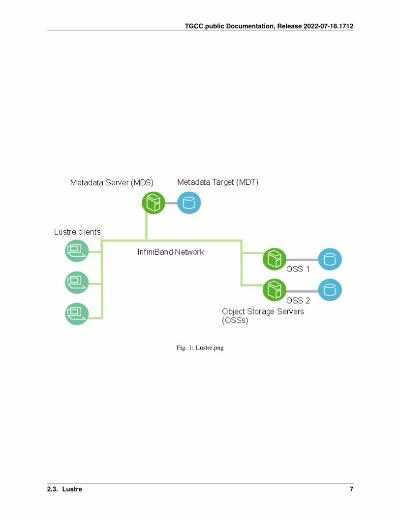
Lustre is a type of parallel distributed file system, commonly used for large-scale cluster computing. It actually relieson a set of multiple I/O servers and the Lustre software presents them as a single unified filesystem.
The major Lustre components are the MDS (MetaData Server) and OSSs (Object Storage Servers). The MDS storesmetadata such as file names, directories, access permissions, and file layout. It is not actually involved in any I/Ooperations. The actual data is stored on the OSSs. Note that one single file can be stored on several OSSs which is oneof the benefits of Lustre when working with large files.
More information on how Lustre works and best practices are described in Lustre best practice.
6 Chapter 2. Supercomputer architecture
TGCC public Documentation, Release 2022-07-18.1712
Fig. 1: Lustre.png
2.3. Lustre 7
TGCC public Documentation, Release 2022-07-18.1712
8 Chapter 2. Supercomputer architecture

CHAPTER
THREE
USER ACCOUNT
Warning: Please refer to internal technical documentation to get information about this subject.
9

TGCC public Documentation, Release 2022-07-18.1712
10 Chapter 3. User account
CHAPTER
FOUR
INTERACTIVE ACCESS
4.1 System access
Warning: Please refer to internal technical documentation to get information about this subject.
4.2 Login nodes usage
When you connect to the supercomputer, you are directed to one of the login nodes of the machine. Many users aresimultaneously connected to these login nodes. Since their resources are shared it is important to respect some standardsof good practice.
4.2.1 Usage limit on login nodes
Login nodes should only be used to interact with the batch manager and to run lightweight tasks. As a rule of thumb,any process or group of processes which would use more CPU power and/or memory than what is available on a basicpersonal computer should not be executed on a login node. For more demanding interactive tasks, you should allocatededicated resources on a compute node.
To ensure a satisfying experience for all users, offending tasks are automatically throttled or killed.
4.2.2 Interactive submission
There are 2 possible ways of accessing computing resources without using a submission script. ccc_mprun -K allowsto create the allocation and the job environment while you are still on the login node. It is useful for MPI tests.ccc_mprun -s opens a shell on a compute node. It is useful for sequential or multi-threaded work that would be toocostly for the login node.
11
TGCC public Documentation, Release 2022-07-18.1712
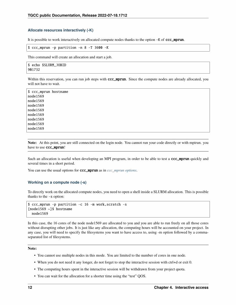
Allocate resources interactively (-K)
It is possible to work interactively on allocated compute nodes thanks to the option -K of ccc_mprun.
$ ccc_mprun -p partition -n 8 -T 3600 -K
This command will create an allocation and start a job.
$ echo $SLURM_JOBID901732
Within this reservation, you can run job steps with ccc_mprun. Since the compute nodes are already allocated, youwill not have to wait.
$ ccc_mprun hostnamenode1569node1569node1569node1569node1569node1569node1569node1569
Note: At this point, you are still connected on the login node. You cannot run your code directly or with mpirun. youhave to use ccc_mprun!
Such an allocation is useful when developing an MPI program, in order to be able to test a ccc_mprun quickly andseveral times in a short period.
You can use the usual options for ccc_mprun as in ccc_mprun options.
Working on a compute node (-s)
To directly work on the allocated compute nodes, you need to open a shell inside a SLURM allocation. This is possiblethanks to the -s option:
$ ccc_mprun -p partition -c 16 -m work,scratch -s[node1569 ~]$ hostnamenode1569
In this case, the 16 cores of the node node1569 are allocated to you and you are able to run freely on all those coreswithout disrupting other jobs. It is just like any allocation, the computing hours will be accounted on your project. Inany case, you will need to specify the filesystems you want to have access to, using -m option followed by a comma-separated list of filesystems.
Note:
• You cannot use multiple nodes in this mode. You are limited to the number of cores in one node.
• When you do not need it any longer, do not forget to stop the interactive session with ctrl+d or exit 0.
• The computing hours spent in the interactive session will be withdrawn from your project quota.
• You can wait for the allocation for a shorter time using the “test” QOS.
12 Chapter 4. Interactive access
TGCC public Documentation, Release 2022-07-18.1712
This is typically used for costly and punctual tasks such as compiling a large code on 16 cores, post-processing oraggregating output data etc.
At any point, you can use the hostname command to check whether you are on a compute node or on a login nodes.
You can use the usual options for ccc_mprun as in ccc_mprun options.
4.2.3 Crontab
Crontab mechanism is available on login nodes in order to execute desired tasks in the background at designated times.A specific version of cron called crontab is provided and can be invoked with the regular crontab command name.crontab adds the ability to manage the crontab content associated to your user account whatever the login node yourare connected to, still having this crontab be executed once (only one login node schedules and executes the commandsyou specify in your crontab).
The command crontab -e edits the file which contains the instructions to be launched, and crontab -r removesthe current crontab. The instructions follow the following format:
mm hh dd MMM DDD task > logfile
where mm, hh, dd, MMM represent the minutes, the hours, the day of the month MMM, and DDD the days of everyweek on which the task ‘task’ is executed. ‘Logfile’ is the log file in which is redirected the standard output. Theperiodicity of the task must be appropriate to the need, and must not be lower than 5 minutes in order to not over solicitthe system. Below are some examples of valid instruction lines:
0 0 * * 1 ccc_msub /path1/regression.sh >> /path2/joblist.sh
will submit every Monday at 0:00 the script of submission regression.sh, and writes the JobID in the file joblist.sh.
*/10 8-18 * * mon,tue,wed,thu,fri clear > /dev/null 2>&1
clears the shell every ten minutes between 8 a.m. and 6 p.m. during the week, without saving the output.
0 10 20 12 * mkdir /path3/annual_report
will create every 20th of December at 10 a.m. the folder ‘annual_report’ in /path3.
4.2. Login nodes usage 13
TGCC public Documentation, Release 2022-07-18.1712
14 Chapter 4. Interactive access
CHAPTER
FIVE
DATA SPACES
All user data are stored on file systems reachable from the supercomputer login and compute nodes. Each file systemhas a purpose: your HOME directory contains user configuration, your SCRATCH directory is intended for temporarycomputational data sets, etc. To prevent over-usage of the file system capacities, limitations/quotas are set on dataspace allocated to users or groups. Except for your HOME directory, which is hosted by a NFS file system, user dataspaces are stored on Lustre file systems. This section provides data usage guidelines that must be followed, since aninappropriate usage of the file systems might badly affect the overall production of the computing center.
5.1 Available file systems
This section introduces the available file systems with their purpose, their quota policy and their recommended usage.
HOME
The HOME is a slow, small file system with backup that can be used from any machine.
Characteristics:
• Type: NFS
• Data transfer rate: low
• Quota: 5GB/user
• Usage: Sources, job submission scripts. . .
• Comments: Data are saved
• Access: from all resources of the center
• Variable: HOME or CCFRHOME
Note:
• HOME is the only file system without limitation on the number of files (quota on inodes)
• The retention time for HOME directories backup is 6 months
• The backup files are under the ~/.snapshot directory
SCRATCH
The SCRATCH is a very fast, big and automatically purged file system.
Characteristics:
• Type: Lustre
15
TGCC public Documentation, Release 2022-07-18.1712
• Data transfer rate: 300 GB/s
• Quota: The quota is defined by group. The command ccc_quota provides information about the quota of thegroups you belong to. By default, a quota of 2 millions inodes and 100 To of disk space is granted for each dataspace.
• Usage: Data, Code output. . .
• Comments: This filesystem is subject to purge
• Access: Local to the supercomputer
• Variable: CCCSCRATCHDIR or CCFRSCRATCH
The purge policy is as follows:
• Files not accessed for 60 days are automatically purged
• Symbolic links are not purged
• Directories that have been empty for more than 30 days are removed
WORK
WORK is a fast, medium and permanent file system (but without backup):
Characteristics:
• Type: Lustre via routers
• Data transfer rate: high (70 GB/s)
• Quota: 5 TB and 500 000 files/group
• Usage: Commonly used file (Source code, Binary. . . )
• Comments: Neither purged nor saved (tar your important data to STORE)
• Access: from all resources of the center
• Variable: CCCWORKDIR or CCFRWORK
Note:
• WORK is smaller than SCRATCH, it’s only managed through quota.
• This space is not purged but not saved (regularly backup your important data as tar files in STORE)
STORE
STORE is a huge storage file system
Characteristics:
• Type: Lustre + HSM
• Data transfer rate: high (200 GB/s)
• Quota: 50 000 files/group, expected file size range 10GB-1TB
• Usage: To store of large files (direct computation allowed in that case) or packed data (tar files. . . )
• Comments: Migration to hsm relies on file modification time: avoid using cp options like -p, -a . . .
• Access: from all resources of the center
• Variable: CCCSTOREDIR or CCFRSTORE
16 Chapter 5. Data spaces
TGCC public Documentation, Release 2022-07-18.1712
• Additional info: Use ccc_hsm status <file> to know whether a file is on disk or tape level, and ccc_hsmget <file> to preload file from tape before a computation
Note:
• STORE has no limit on the disk usage (quota on space)
• STORE usage is monitored by a scoring system
• An HSM (Hierarchical Storage Management) is a data storage system which automatically moves data betweenhigh-speed and low-speed storage media. In our case, the high speed device is a Lustre file system and the lowspeed device consists of magnetic tape drives. Data copied to the HSM filesystem will be moved to magnetictapes (usually depending on the modification date of the files). Once the data is stored on tape, accessing it willbe slower.
TMP
TMP is a local, fast file system but of limited size.
Characteristics:
• Type: zram (RAM)
• Data transfer rate: very high (>1Go/s) and very low latency
• Size: 16 Go
• Usage: Temporary files during a job
• Comments: Purge after each job
• Access: Local within each node
• Variable: CCCTMPDIR or CCFRTMP
Note:
• TMP allow fast write and read for local needs.
• TMP is local to the node. Only jobs/processes within the same node have access to the same files.
• Write files in TMP will reduce the amount of available RAM.
SHM
SHM is a very fast, local file system but of limited size.
Characteristics:
• Type: tmpfs (RAM, block size 4Ko)
• Data transfer rate: very high (>1Go/s) and very low latency
• Size: 50% of RAM (ie: 94 Go on skylake)
• Usage: Temporary files during compute; can be used as a large cache
• Comments: Purge after each job
• Access: Local within each node
• Variable: CCCSHMDIR
5.1. Available file systems 17
TGCC public Documentation, Release 2022-07-18.1712
Note:
• SHM allow very fast file access.
• SHM is local to the node. Only jobs/processes within the same node have access to the same files.
• Write files in SHM will reduce the amount of available RAM.
5.2 Quota
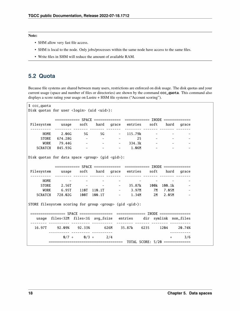
Because file systems are shared between many users, restrictions are enforced on disk usage. The disk quotas and yourcurrent usage (space and number of files or directories) are shown by the command ccc_quota. This command alsodisplays a score rating your usage on Lustre + HSM file systems (“Account scoring”).
$ ccc_quotaDisk quotas for user <login> (uid <uid>):
============ SPACE ============= ============ INODE =============Filesystem usage soft hard grace entries soft hard grace---------- -------- ------- ------- ------- -------- ------- ------- -------
HOME 2.06G 5G 5G - 115.79k - - -STORE 674.28G - - - 25 - - -WORK 79.44G - - - 334.3k - - -
SCRATCH 845.93G - - - 1.06M - - -
Disk quotas for data space <group> (gid <gid>):
============ SPACE ============= ============ INODE =============Filesystem usage soft hard grace entries soft hard grace---------- -------- ------- ------- ------- -------- ------- ------- -------
HOME - - - - - - - -STORE 2.56T - - - 35.87k 100k 100.1k -WORK 6.95T 110T 110.1T - 3.97M 7M 7.05M -
SCRATCH 728.02G 100T 100.1T - 1.34M 2M 2.05M -
STORE filesystem scoring for group <group> (gid <gid>):
================= SPACE ================ ============== INODE ===============usage files<32M files<1G avg_fsize entries dir symlink non_files
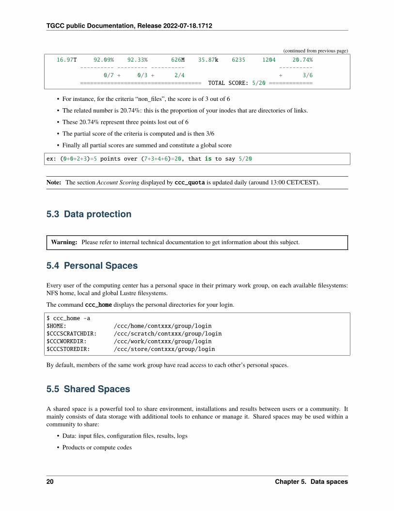
-------- ---------- --------- ---------- -------- ------- -------- ----------16.97T 92.09% 92.33% 626M 35.87k 6235 1204 20.74%
---------- --------- ---------- ----------0/7 + 0/3 + 2/4 + 3/6
==================================== TOTAL SCORE: 5/20 =============
18 Chapter 5. Data spaces
TGCC public Documentation, Release 2022-07-18.1712
5.2.1 Disk quotas
Three parameters govern the disk quotas:
• soft limit: when your usage reaches this limit you will be warned.
• hard limit: when your usage reaches this limit you will be unable to write new files.
• grace period: the period during which you can exceed the soft limit.
Within the computing center, the quotas have been defined as follows:
• the grace period is 1 week. It means that once you have reached the soft limit, a countdown starts for a week. Bythe end of the countdown, if you have not brought your quota under the soft limit, you will not be able to createnew files anymore. Once you get back under the soft limit, the countdown is reset.
• soft limit and hard limit are almost always the same, which means that checking your current usage to be belowthis limit is enough.
• those limits have been set on both the number of files (inode) and the data usage (space) for WORK andSCRATCH.
• those limits have been set only on the data usage (space) for HOME.
• those limits have been set only on the number of files (inode) for Lustre + HSM file systems (CCCSTOREDIR).
• Lustre + HSM file systems (CCCSTOREDIR) have a scoring system instead of space limitations.
Note: The section Disk quotas displayed by ccc_quota is updated in real-time.
5.2.2 Account scoring
On Lustre + HSM file systems (CCCSTOREDIR), a score reflects how close you are from the recommended usage.
4 criteria are defined and are each granted a certain amount of points. Here are those criteria:
• inodes should be regular files (not directories nor symbolic links) for 6 points,
• files should be bigger than 32MB for 7 points,
• files should be bigger than 1GB for 3 points,
• the average file size should be high enough for 4 points. More specifically, with 64MB, 128MB, 1GB and 8GBas limits, you get one point per limit exceeded by your average file size. For example, an average file size of 2GBwill give you a partial score of 3/4.
The command ccc_quota shows how well you match the criteria in the Account Scoring section:
• current usage (space and inodes)
• percentages of files not matching the criteria
• global score and the partial scores.
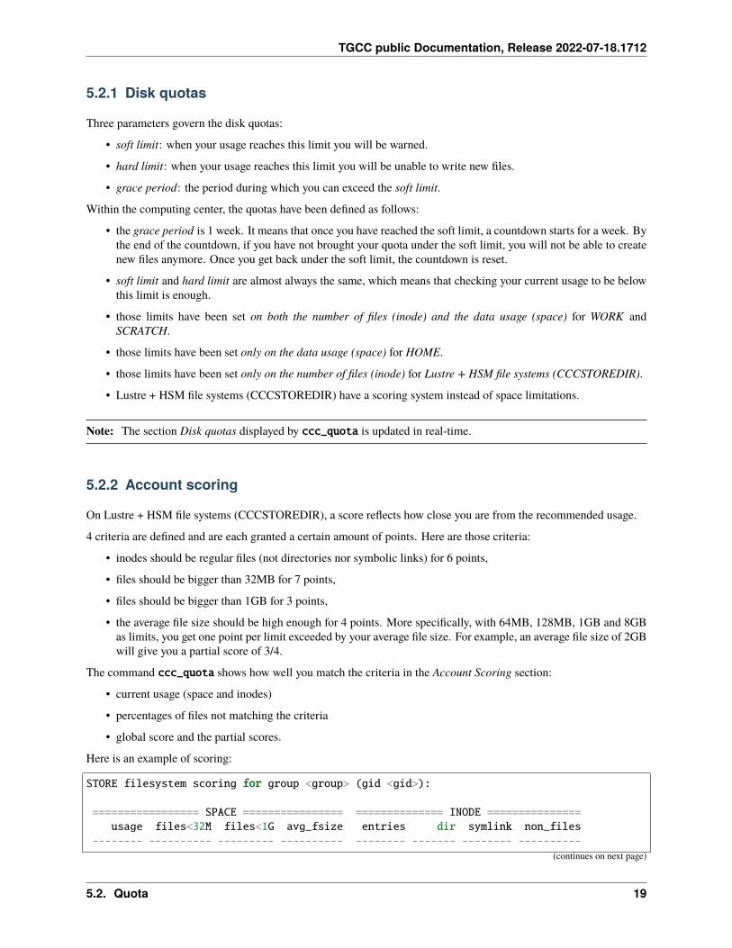
Here is an example of scoring:
STORE filesystem scoring for group <group> (gid <gid>):
================= SPACE ================ ============== INODE ===============usage files<32M files<1G avg_fsize entries dir symlink non_files
-------- ---------- --------- ---------- -------- ------- -------- ----------(continues on next page)
5.2. Quota 19
TGCC public Documentation, Release 2022-07-18.1712
(continued from previous page)
16.97T 92.09% 92.33% 626M 35.87k 6235 1204 20.74%---------- --------- ---------- ----------
0/7 + 0/3 + 2/4 + 3/6==================================== TOTAL SCORE: 5/20 =============
• For instance, for the criteria “non_files”, the score is of 3 out of 6
• The related number is 20.74%: this is the proportion of your inodes that are directories of links.
• These 20.74% represent three points lost out of 6
• The partial score of the criteria is computed and is then 3/6
• Finally all partial scores are summed and constitute a global score
ex: (0+0+2+3)=5 points over (7+3+4+6)=20, that is to say 5/20
Note: The section Account Scoring displayed by ccc_quota is updated daily (around 13:00 CET/CEST).
5.3 Data protection
Warning: Please refer to internal technical documentation to get information about this subject.
5.4 Personal Spaces
Every user of the computing center has a personal space in their primary work group, on each available filesystems:NFS home, local and global Lustre filesystems.
The command ccc_home displays the personal directories for your login.
$ ccc_home -a$HOME: /ccc/home/contxxx/group/login$CCCSCRATCHDIR: /ccc/scratch/contxxx/group/login$CCCWORKDIR: /ccc/work/contxxx/group/login$CCCSTOREDIR: /ccc/store/contxxx/group/login
By default, members of the same work group have read access to each other’s personal spaces.
5.5 Shared Spaces
A shared space is a powerful tool to share environment, installations and results between users or a community. Itmainly consists of data storage with additional tools to enhance or manage it. Shared spaces may be used within acommunity to share:
• Data: input files, configuration files, results, logs
• Products or compute codes
20 Chapter 5. Data spaces
TGCC public Documentation, Release 2022-07-18.1712
5.5.1 Accessibility and procedures
Warning: Please refer to internal technical documentation to get information about this subject.
5.5.2 Implementation
File systems
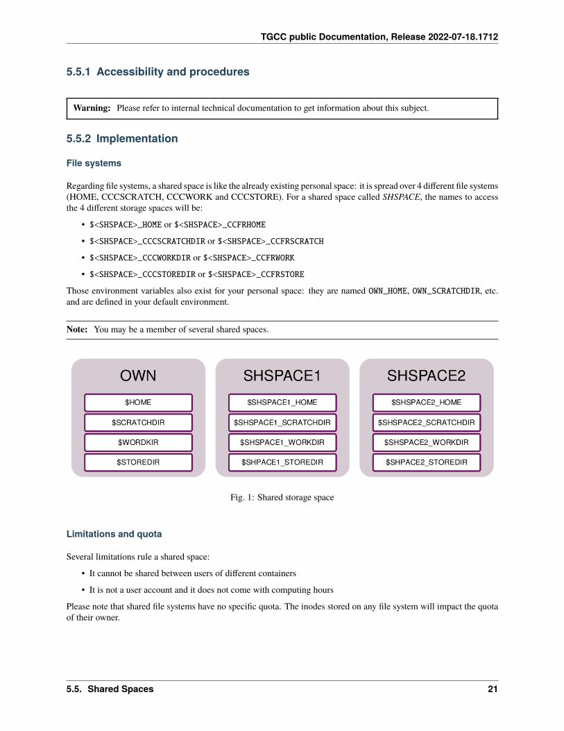
Regarding file systems, a shared space is like the already existing personal space: it is spread over 4 different file systems(HOME, CCCSCRATCH, CCCWORK and CCCSTORE). For a shared space called SHSPACE, the names to accessthe 4 different storage spaces will be:
• $<SHSPACE>_HOME or $<SHSPACE>_CCFRHOME
• $<SHSPACE>_CCCSCRATCHDIR or $<SHSPACE>_CCFRSCRATCH
• $<SHSPACE>_CCCWORKDIR or $<SHSPACE>_CCFRWORK
• $<SHSPACE>_CCCSTOREDIR or $<SHSPACE>_CCFRSTORE
Those environment variables also exist for your personal space: they are named OWN_HOME, OWN_SCRATCHDIR, etc.and are defined in your default environment.
Note: You may be a member of several shared spaces.
Fig. 1: Shared storage space
Limitations and quota
Several limitations rule a shared space:
• It cannot be shared between users of different containers
• It is not a user account and it does not come with computing hours
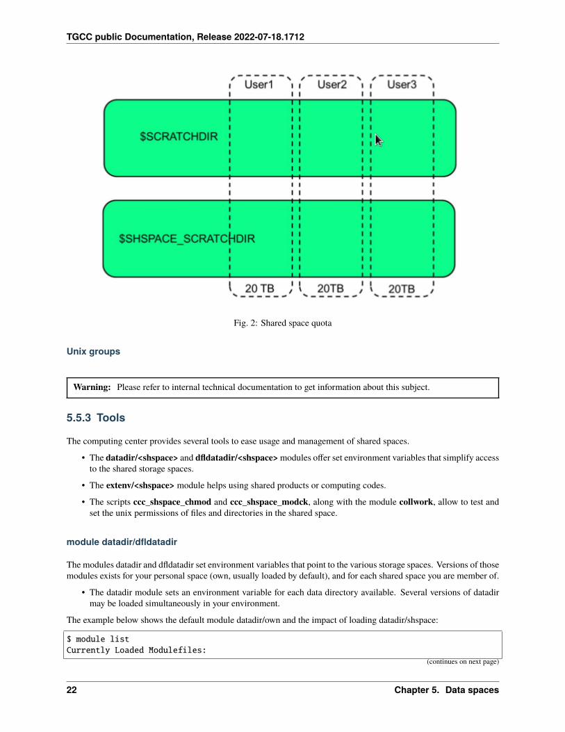
Please note that shared file systems have no specific quota. The inodes stored on any file system will impact the quotaof their owner.
5.5. Shared Spaces 21
TGCC public Documentation, Release 2022-07-18.1712
Fig. 2: Shared space quota
Unix groups
Warning: Please refer to internal technical documentation to get information about this subject.
5.5.3 Tools
The computing center provides several tools to ease usage and management of shared spaces.
• The datadir/<shspace> and dfldatadir/<shspace> modules offer set environment variables that simplify accessto the shared storage spaces.
• The extenv/<shspace> module helps using shared products or computing codes.
• The scripts ccc_shspace_chmod and ccc_shspace_modck, along with the module collwork, allow to test andset the unix permissions of files and directories in the shared space.
module datadir/dfldatadir
The modules datadir and dfldatadir set environment variables that point to the various storage spaces. Versions of thosemodules exists for your personal space (own, usually loaded by default), and for each shared space you are member of.
• The datadir module sets an environment variable for each data directory available. Several versions of datadirmay be loaded simultaneously in your environment.
The example below shows the default module datadir/own and the impact of loading datadir/shspace:
$ module listCurrently Loaded Modulefiles:
(continues on next page)
22 Chapter 5. Data spaces
TGCC public Documentation, Release 2022-07-18.1712
(continued from previous page)
1) ccc 2) datadir/own 3) dfldatadir/own
$ echo $OWN_CCCWORKDIR/ccc/work/contxxx/grp1/user1
$ module load datadir/shspaceload module datadir/shspace (Data Directory)
$ echo $SHSPACE_CCCWORKDIR/ccc/work/contxxx/shspace/shspace
• The dfldatadir module sets the default environment variables for the various storage spaces (CCCSCRATCHDIR,CCCWORKDIR, CCCSTOREDIR and their CCFR equivalent).
Only one version of dfldatadir can be loaded at a time.
This example shows how to use dfldatadir:
$ module listCurrently Loaded Modulefiles:1) ccc 2) datadir/own 3) dfldatadir/own
$ echo $CCCWORKDIR/ccc/work/contxxx/grp1/user1
By default, $CCCWORKDIR (and its CCFR’s equivalent $CCFRWORK) points to your own work directory.
$ module switch dfldatadir/own dfldatadir/shspaceunload module dfldatadir/own (Default Data Directory)unload module datadir/own (Data Directory)load module dfldatadir/shspace (Default Data Directory)
Once dfldatadir/shspace is loaded instead of dfldatadir/own, $CCCWORKDIR (and $CCFRWORK) points to the work direc-tory shared by shspace.
$ echo $CCCWORKDIR/ccc/work/contxxx/shspace/shspace
Generic variables are set by the dfldatadir module, which point to the datadir/shspace variables without mentioning aspecific shspace name. This can be useful in order to create generic scripts adapted to different projects.
$ echo $ALL_CCCWORKDIR/ccc/work/contxxx/shspace/shspace
5.5. Shared Spaces 23
TGCC public Documentation, Release 2022-07-18.1712
Environment extension
The extenv module extends the current user environment. It defines a common environment for all users of a sharedspace.
Loading the extenv module will:
• Set environment variables defining the path to shared products and module files (SHSPACE_PRODUCTSHOME,SHSPACE_MODULEFILES, SHSPACE_MODULESHOME)
• Execute an initialization script
• Add shared modules to the available modules
The environment extension mechanisms uses specific paths. Products installed in the <shspace> shared space shouldbe installed in $SHSPACE_PRODUCTSHOME and the corresponding module files should be in $SHSPACE_MODULEFILES.
Initialization file
If a file named init is found in the path defined by $SHSPACE_MODULESHOME, then it is executed each time the ex-tenv/<shspace> module is loaded. This may be helpful to define other common environment variables or to add pre-requisites on modules to be used by the community.
For instance the following example defines two environment variables: one is the directory containing in-put files (SHSPACE_INPUTDIR), and the other is the result directory (SHSPACE_RESULTDIR). It also adds$SHSPACE_PRODUCTSHOME/tools/bin to the PATH so that the tools installed in $SHSPACE_PRODUCTSHOME/tools/bin are easily available.
$ cat $SHSPACE_MODULESHOME/initsetenv SHSPACE_INPUTDIR "$env(SHSPACE_CCCWORKDIR)/in"setenv SHSPACE_RESULTDIR "$env(SHSPACE_CCCSCRATCHDIR)/res"append-path PATH "$env(SHSPACE_PRODUCTSHOME)/tools/bin"
Modules
After the module extenv/<shspace> is loaded, all the module files located in $SHSPACE_MODULEFILES become visibleto the module command. For each product, there should be one module file per version.
For example, if you create specific modules in the shared environment in the following paths:
$ find $SHSPACE_MODULEFILES/ccc/contxxx/home/shspace/shspace/products/modules/modulefiles/ccc/contxxx/home/shspace/shspace/products/modules/modulefiles/code1/ccc/contxxx/home/shspace/shspace/products/modules/modulefiles/tool2/ccc/contxxx/home/shspace/shspace/products/modules/modulefiles/libprod/ccc/contxxx/home/shspace/shspace/products/modules/modulefiles/libprod/1.0/ccc/contxxx/home/shspace/shspace/products/modules/modulefiles/libprod/2.0
Then, those modules will be visible and accessible once the extenv/<shspace> module is loaded.
$ module load extenv/shspaceload module extenv/shspace (Extra Environment)$ module avail---------------- /opt/Modules/default/modulefiles/applications -----------------abinit/x.y.z gaussian/x.y.z openfoam/x.y.z
(continues on next page)
24 Chapter 5. Data spaces
TGCC public Documentation, Release 2022-07-18.1712
(continued from previous page)
[...]-------------------- /opt/Modules/default/modulefiles/tools --------------------advisor/x.y.z ipython/x.y.z r/x.y.z[...]-------- /ccc/contxxx/home/shspace/shspace/products/modules/modulefiles --------code1 libprod/1.0 libprod/2.0 tool2
$ module load tool2$ module listCurrently Loaded Modulefiles:1) ccc 3) dfldatadir/own 5) extenv/shspace2) datadir/own 4) datadir/shspace 6) tool2
Let us consider the example of a product installed in the shared space. The program is called prog. Its version isversion. It depends on the product dep. The product should be installed in the directory $SHSPACE_PRODUCTSHOME/prog-version. The syntax of its module file $SHSPACE_MODULEFILES/prog/version would be:
#%Module1.0# Software descriptionset version "version"set whatis "PROG"set software "prog"set description "<description>"
# Conflictconflict "$software"
# Prereqprereq dep
# load head common functions and behaviorsource $env(MODULEFILES)/.headcommon# Loads software's environment
# application-specific variablesset prefix "$env(SHSPACE_PRODUCTSHOME)/$software-$version"set libdir "$prefix/lib"set incdir "$prefix/include"set docdir "$prefix/doc"
# compilerwrappers-specific variablesset ldflags "<ldflags>"
append-path PATH "$bindir"append-path LD_LIBRARY_PATH "$libdir"
setenv VARNAME "VALUE"
# load common functions and behaviorsource $env(MODULEFILES)/.common
• Setting the local variables prefix, libdir, incdir and docdir will create the environment variablesPROG_ROOT, PROG_LIBDIR, PROG_INCDIR and PROG_DOCDIR when the module is loaded. You can also de-
5.5. Shared Spaces 25
TGCC public Documentation, Release 2022-07-18.1712
fine any environment variable needed by the software as the example does for VARNAME.
• Inter module dependencies are now handled automatically with the prereq keyword. That way, any time themodule is loaded, its dependencies are loaded if necessary.
We recommend the use of the previous example as a template for all your module files. If you use the recommendedpath for all installations ($SHSPACE_PRODUCTSHOME/<software>-<version>), you can keep that template as it is.Just specify the right software and version and the potential VARNAME environment variables you want to define forthe software.
Using that template will ensure that your module behaves the same way as the default modules and that all the availablemodule commands will work for you.
Module collection
The collection mechanism allows to define a set of modules to be loaded either automatically when starting a session,through the default collection or manually with module restore [collection_name].
Along with datadir, dfldatadir and extenv, the aim of this collections is to replace all users configurations that may havebeen done up to now in the shell configuration files. (.bashrc, .bash_profile, etc)
Here are the useful commands to manage collections:
• To create a collection containing the modules currently loaded in your environment:
module save [collection_name]
If [collection_name] is not specified, it will impact the default collection.
• To list available collections:
module savelist
• To load a saved collection:
module restore [collection_name]
If [collection_name] is not specified, the default collection will be loaded.
Those collections are stored in the users home, just like shell configuration scripts.
Let us say you have a product Tool2 installed in your shared extended environment. Here is how you would add it toyour default collection:
$ module listCurrently Loaded Modulefiles:1) ccc 2) datadir/own 3) dfldatadir/own
Load all necessary modules to access your shared product correctly.
$ module load datadir/shspaceload module datadir/shspace (Data Directory)$ module load extenv/shspaceload module extenv/shspace (Extra Environment)$ module load tool2load module tool2 (TOOL2)$ module listCurrently Loaded Modulefiles:
(continues on next page)
26 Chapter 5. Data spaces
TGCC public Documentation, Release 2022-07-18.1712
(continued from previous page)
1) ccc 3) dfldatadir/own 5) extenv/shspace2) datadir/own 4) datadir/shspace 6) tool2
Use module save to make the current environment the default one.
$ module save
After that, every time you will connect to your account, those will be the modules loaded by default.
We highly recommend the use of collections instead of adding calls to module load in shell configuration files. Acall to module load takes non negligible time whether the module was already loaded or not. And when they arespecified in ~/.bashrc, they run for each bash script or shell execution. On the contrary, a collection is only loaded ifthe environment has not yet been initialized. Therefore, using collections will fasten connections and script executions.
Note: To ensure the correct setting of your user environment, make sure
• That the file ~/.bashrc contains:
if [ -f /etc/bashrc ]; then. /etc/bashrcfi
• That the file ~/.bash_profile contains:
if [ -f ~/.bashrc ]; then. ~/.bashrcfi
Managing permissions
Warning: Please refer to internal technical documentation to get information about this subject.
5.6 Parallel file system usage monitoring
Some general best practice rules should be met when using the available file systems. They are specified in Recom-mended data usage on parallel file system.
Inappropriate usage of parallel file systems is monitored, as it may badly affect overall performances. Several inappro-priate practices are tracked down.
5.6.1 Too many small files on CCCSTOREDIR
File size has to be constrained. The following is considered inappropriate:
• Average size of files below 50MB (see the column “avg_fsize(MB)” from ccc_quota)
• Percentage of files lower than 32MB higher than 80% (see the column “files<32M” from ccc_quota)
Once a week if rules are not followed, actions are triggered until situation is back to normal:
• Week 1: The user is informed by mail.
• Week 2: The user is informed by mail.
5.6. Parallel file system usage monitoring 27
TGCC public Documentation, Release 2022-07-18.1712
• Week 3: The user is informed by mail and his submissions are locked.
• Week 4: The user is informed by mail.
• Week 5: The user is informed by mail, his account is locked and his files can be removed.
5.6.2 Too many files in a directory on SCRATCH, WORK and STORE
Directories with more than 50000 entries (files or directories) at the root level is inappropriate.
Once a week if this rule is not followed, actions are triggered until situation is back to normal:
• Week 1: The user is informed by mail.
• Week 2: The user is informed by mail.
• Week 3: The user is informed by mail and his submissions are locked.
• Week 4: The user is informed by mail.
• Week 5: The user is informed by mail, his account is locked and his files can be removed.
28 Chapter 5. Data spaces
CHAPTER
SIX
DATA TRANSFERS
6.1 File transfer
The center provides several means of transferring data to and from its various resources.
• On Unix-like OSes (for instance Linux or Mac OS X) use the scp or rsync commands.
• On Windows, several clients exist. For example PSCP or WinSCP
Note: SFTP (SSH File Transfer Protocol), which is used for example by WinSCP, is disabled for security reasons onPRACE and FR login nodes.
Call the transfer routines from your local machine (local_host). Here are the different ways to copy data from or tothe supercomputer login node (remote_host). The remote host depends on the type of project. It is the one used forSSH connections (see Interactive access for more details). Hereafter, remote_dir represents a valid directory on theremote host.
6.1.1 scp
scp copies files between hosts on a network. It uses ssh for data transfer, with the same authentication and the samesecurity as ssh.
To transfer data from local machine to remote machine:
$ scp [options] <local_files> <login>@<remote_host>:<remote_dir>
To transfer data from remote machine to local machine:
$ scp [options] <login>@<remote_host>:<remote_dir>/<files> <local_dir>
Basic options are -v for verbose mode and -r to copy directories. For more information, type man scp from thecommand line.
29
TGCC public Documentation, Release 2022-07-18.1712
6.1.2 rsync
rsync synchronizes two sets of files across a network. It sends only the differences between the source files and thedestination files.
To transfer data from local machine to remote machine:
$ rsync -e ssh -avz <local_files> <login>@<remote_host>:<remote_dir>
To transfer data from remote machine to local machine:
$ rsync -e ssh -avz <login>@<remote_host>:<remote_dir>/<files> <local_dir>
For more information, type man rsync from the command line.
Note: Transferring data from or to the supercomputer may be more efficient when using archives instead of manysmall files.
6.1.3 sftp
sftp connects on a remote host, then can transfer files on both directions. It uses ssh for data transfer, with the sameauthentication and the same security as ssh.
To connect on a remote host:
$ sftp [options] <login>@<remote_host>
An usual option is -r to copy directories. For more information, type man sftp from the command line.
Once logged in, to transfer data from the remote host to the local host:
$ sftp> get [options] <remote_path> <local_path>
And to transfer data from the local host to the remote host:
$ sftp> put [options] <local_path> <remote_path>
If you haven’t used the -r option with the sftp command, you can use it directly with get and put. For moreinformation, type help from the sftp prompt, or man sftp from the command line.
6.1.4 parallel sftp
To speed up file transfer, you can use psftp, a tool developed by CEA. psftp uses parallel sftp to make file transfers.You can install it locally by following the dedicated website: https://github.com/cea-hpc/openssh-portable
Note:
• psftp is not tested on Windows and MacOS.
• psftp is only useful when your transfer overuses a CPU on one of the hosts (local or remote computer). On amodern processor, it happens when the transfer bandwidth reaches ± 1Gbps (please double check if the networklink between both nodes can use more than 1Gbps of bandwitdh).
30 Chapter 6. Data transfers
TGCC public Documentation, Release 2022-07-18.1712
psftp is installed on login nodes of CEA clusters. Its usage is identical as sftp, except the option -n which let youchoose the number of ssh connections used for the parallel transfer.
For example, to make a parallel transfer with 5 ssh connections:
$ psftp -n 5 <login>@<remote_host>
If one sftp transfer is limited at 1Gbps, this transfer will use at most 5Gbps.
6.2 CCFR infrastructure
Warning: Please refer to internal technical documentation to get information about this subject.
6.3 PRACE infrastructure
Warning: Please refer to internal technical documentation to get information about this subject.
6.2. CCFR infrastructure 31

TGCC public Documentation, Release 2022-07-18.1712
32 Chapter 6. Data transfers
CHAPTER
SEVEN
ENVIRONMENT MANAGEMENT
Traditional Unix way to manage environment usually involves editing your ~/.bashrc and/or sourcing software-specific files. This methodology can be error-prone due to inconsistent definitions and hardly let users dynamicallyenable or change the software they want to use. To dynamically manage your environment and pick up the neededsoftware among the large software catalog provided, the module command is provided from the Environment Modulesproject.
7.1 What is module
module is a user interface providing dynamic modification of your environment via modulefiles. module allows tochange easily the shell environment by initializing, modifying or unsetting environment variables.
Each modulefile contains the information needed to configure the shell for an application. Once the module is initial-ized, the environment can be modified on a per-module basis using the module command which interprets modulefiles.Typically modulefiles instruct the module command to alter or set shell environment variables such as PATH, MANPATH,etc. The modulefiles are added to and removed from the current environment by the user.
On the computing center, it is typically used to:
• define your user environment ($HOME, $CCCSCRATCHDIR, etc.);
• easily get access to third-party softwares in different versions (ex: Intel compilers, GCC, MPI librairies, etc.);
• handle the potential conflicts an requirements between software.
Modulefiles are basically provided by the computing center staff to get access to the installed software and to the systemproperties. In addition you may have your own modulefiles to supplement the already provided modulefiles.
7.2 Module actions
Major kind of actions of the module command are described below. To get a full reference of the available moduleactions, you can either
• display the command usage message (module -h)
• look at the man page (man module)
• or even try the command auto-completion
33
TGCC public Documentation, Release 2022-07-18.1712
7.2.1 Listing / Searching modulefiles
Knowing current environment state:
• module list shows the current state of your environment, which means to display all the modules currentlyloaded
Querying modulefiles catalog:
• module avail displays all available modules (modules suffixed by @ are aliases)
• module avail --default reduces the regular avail output by only displaying the available default versions
• module avail --latest in the same way displays only the available latest versions
• module avail mpi shows the available mpi modulefiles
Printing modulefile information:
• module help netcdf shows software description for default netcdf modulefile
• module help hdf5/x.y.z shows software description for a specific hdf5 modulefile
• module show mkl displays software description plus environment definition for the default mkl
• module show python/x.y.z displays as above description and environment definition but for a specific ver-sion
Searching for modulefiles:
• module whatis papi prints for each version of papi product a one-liner description and its associated keywords
• module show products/keywords prints products/keywords modulefile description which lists all keywordsin-use by available modulefiles
• module search profiler searches for all products whose name, one-liner description or keywords match theprofiler search string
7.2.2 Loading / Unloading modulefiles
Adding modulefile(s) to the list of currently loaded modules:
• module load fftw3 loads the default version of fftw3 product or its latest version if no default version isexplicitly set
• module load visit/x.y.z loads specific version x.y.z of visit
• module load intel hdf5 netcdf loads multiple modulefiles in one command
Note: On interactive shells, module auto-completion is enabled and can help you to find the name of modulefiles youwant to load, unload or switch
Removing modulefile(s) from your current environment:
• module unload visit unloads loaded version of visit modulefile
• module unload netcdf hdf5 unloads multiple products in one command
• module purge unloads all loaded modulefiles
Note: All these load, unload, switch commands returns 0 on success or 1 elsewhere
34 Chapter 7. Environment management
TGCC public Documentation, Release 2022-07-18.1712
Switching from one version of a modulefile to another:
• module switch intel intel/x.y.z unloads currently loaded intel modulefile then loads version x.y.z
Note: The module command will automatically satisfy modulefile prerequisites. When loading a modulefile, all themodulefiles it declares as prerequisite are loaded prior to its own load. When unloading a modulefile, all the modulefilesit declares as prerequisite that have been automatically loaded as dependency are automatically unloaded after the initialmodulefile unload.
7.2.3 Saving and restoring modulefile collections
A modulefile collection corresponds to saved state of your module environment you can restore whenever you want.A collection is composed of an ordered set of modulefiles which are the currently loaded modulefiles at the time ofsaving this collection. When a collection is restored, currently loaded modulefiles are unloaded to then load the set ofmodulefiles defined in the collection in the same loading order.
You can own any number of collections you want, which gives you the ability to easily switch between a productionenvironment and a development environment or between a visualization environment and a debugging one, for instance.
Saving modulefile collections
• module save development saves the current list of loaded modules in the collection named development
• module save saves the current list of loaded modules in the default collection
Listing saved modulefile collections
• module savelist lists all previously saved modulefile collections
Restoring saved modulefile collections:
• module restore development restores the collection named development, by unloading currently loadedmodulefiles then loading the modulefiles defined in the collection to restore the same ordered list of loadedmodulefiles
• module restore restores the default modulefile collection
7.3 Initialization and scope
Depending on shell mode, the module environment is initialized and propagated in different ways. In all cases, themodule command is defined and a minimal environment is set. This minimal environment is composed of the defaultpaths to the modulefiles provided by the computing center staff and the mandatory modulefiles ccc and dfldatadirloaded. Then on interactive shell:
1. all module output messages are set to be redirected to stdout
2. module command auto-completion is enabled
3. your module collection named default is restored if it exists
On non-interactive shell following initialization is done after minimal environment setup:
1. all module output messages are let on stderr
2. module message at load or unload is disabled
3. your module collection named non-interactive is restored if it exists
7.3. Initialization and scope 35
TGCC public Documentation, Release 2022-07-18.1712
7.3.1 Interactive or non-interactive ?
Interactive shell initialization is obtained when:
• you connect to the supercomputer or to a given node within the supercomputer to get a login shell
• you run an interactive job
Non-interactive shell initialization is obtained elsewhere, which means when:
• a batch job starts
• you remotely execute a command (with SSH) on the supercomputer or on a node within the supercomputer
7.3.2 Scope of your environment
Your environment is initialized or re-initialized in the conditions previously described, which means each time youconnect to the supercomputer or from one node to another within the supercomputer your environment is reset to itsdefault. It is also the case when the batch scheduler starts one of your batch job: by default the environment at the timeof the job submission is not restored so the environment of this batch job is initialized as a non-interactive environment.
Once initialized, each load or unload of modulefile modifies the environment of the current shell, its subsequent sub-shells and jobs. So each sub-shell and script launched will inherit the environment from its parent shell. However toguaranty the module function to still be defined in sub-shells and script launched, please ensure that /etc/bashrcconfiguration is loaded in your ~/.bashrc local configuration file, for instance with:
# Source global definitionsif [ -f /etc/bashrc ]; then
. /etc/bashrcfi
Regarding interactive jobs, the environment obtained at the start of this kind of job is the one set when you call forthese interactive jobs. Which means all the modulefiles loaded prior to the execution of an interactive job will be stillloaded once this interactive job session will be established.
7.4 Major modulefiles
Modulefiles provided by the computing center staff are spread across categories to sort them by product function. Thesecategories are applications, compilers, environment, libraries, tools, parallel and graphics. They represent the typeof software, except for parallel and graphics categories which are transversal to the other categories and are made topromote these kind of software.
The environment category is a bit special as it does not contain modulefile definition for product like the other categories.A modulefile from the environment category defines aspects relative to the system or configuration properties for agroup of user that can access and use these system functions.
Some modulefiles from the environment category shape environment usages and possibilities. These major modulefilesare described below.
36 Chapter 7. Environment management
TGCC public Documentation, Release 2022-07-18.1712
7.4.1 ccc
cccmodulefile defines global system variables and aliases needed to get a functional user environment. This modulefileis the first to be loaded in user environment and its load is done within default environment load. It is mandatory andthus cannot be unloaded.
7.4.2 datadir
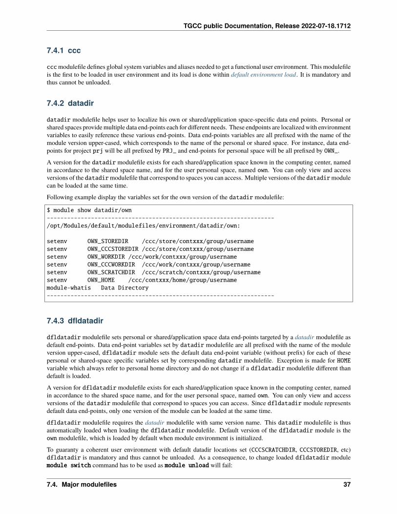
datadir modulefile helps user to localize his own or shared/application space-specific data end points. Personal orshared spaces provide multiple data end-points each for different needs. These endpoints are localized with environmentvariables to easily reference these various end-points. Data end-points variables are all prefixed with the name of themodule version upper-cased, which corresponds to the name of the personal or shared space. For instance, data end-points for project prj will be all prefixed by PRJ_ and end-points for personal space will be all prefixed by OWN_.
A version for the datadir modulefile exists for each shared/application space known in the computing center, namedin accordance to the shared space name, and for the user personal space, named own. You can only view and accessversions of the datadirmodulefile that correspond to spaces you can access. Multiple versions of the datadirmodulecan be loaded at the same time.
Following example display the variables set for the own version of the datadir modulefile:
$ module show datadir/own-------------------------------------------------------------------/opt/Modules/default/modulefiles/environment/datadir/own:
setenv OWN_STOREDIR /ccc/store/contxxx/group/usernamesetenv OWN_CCCSTOREDIR /ccc/store/contxxx/group/usernamesetenv OWN_WORKDIR /ccc/work/contxxx/group/usernamesetenv OWN_CCCWORKDIR /ccc/work/contxxx/group/usernamesetenv OWN_SCRATCHDIR /ccc/scratch/contxxx/group/usernamesetenv OWN_HOME /ccc/contxxx/home/group/usernamemodule-whatis Data Directory-------------------------------------------------------------------
7.4.3 dfldatadir
dfldatadir modulefile sets personal or shared/application space data end-points targeted by a datadir modulefile asdefault end-points. Data end-point variables set by datadir modulefile are all prefixed with the name of the moduleversion upper-cased, dfldatadir module sets the default data end-point variable (without prefix) for each of thesepersonal or shared-space specific variables set by corresponding datadir modulefile. Exception is made for HOMEvariable which always refer to personal home directory and do not change if a dfldatadir modulefile different thandefault is loaded.
A version for dfldatadir modulefile exists for each shared/application space known in the computing center, namedin accordance to the shared space name, and for the user personal space, named own. You can only view and accessversions of the datadir modulefile that correspond to spaces you can access. Since dfldatadir module representsdefault data end-points, only one version of the module can be loaded at the same time.
dfldatadir modulefile requires the datadir modulefile with same version name. This datadir modulefile is thusautomatically loaded when loading the dfldatadir modulefile. Default version of the dfldatadir module is theown modulefile, which is loaded by default when module environment is initialized.
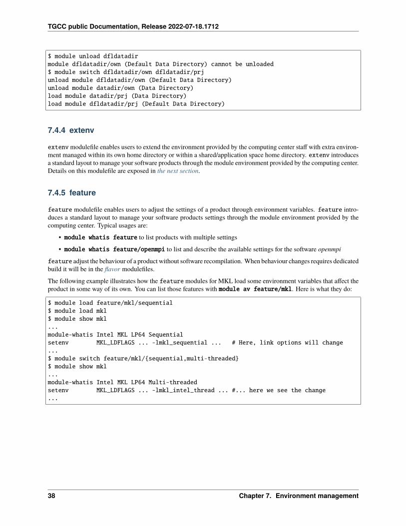
To guaranty a coherent user environment with default datadir locations set (CCCSCRATCHDIR, CCCSTOREDIR, etc)dfldatadir is mandatory and thus cannot be unloaded. As a consequence, to change loaded dfldatadir modulemodule switch command has to be used as module unload will fail:
7.4. Major modulefiles 37
TGCC public Documentation, Release 2022-07-18.1712
$ module unload dfldatadirmodule dfldatadir/own (Default Data Directory) cannot be unloaded$ module switch dfldatadir/own dfldatadir/prjunload module dfldatadir/own (Default Data Directory)unload module datadir/own (Data Directory)load module datadir/prj (Data Directory)load module dfldatadir/prj (Default Data Directory)
7.4.4 extenv
extenv modulefile enables users to extend the environment provided by the computing center staff with extra environ-ment managed within its own home directory or within a shared/application space home directory. extenv introducesa standard layout to manage your software products through the module environment provided by the computing center.Details on this modulefile are exposed in the next section.
7.4.5 feature
feature modulefile enables users to adjust the settings of a product through environment variables. feature intro-duces a standard layout to manage your software products settings through the module environment provided by thecomputing center. Typical usages are:
• module whatis feature to list products with multiple settings
• module whatis feature/openmpi to list and describe the available settings for the software openmpi
feature adjust the behaviour of a product without software recompilation. When behaviour changes requires dedicatedbuild it will be in the flavor modulefiles.
The following example illustrates how the feature modules for MKL load some environment variables that affect theproduct in some way of its own. You can list those features with module av feature/mkl. Here is what they do:
$ module load feature/mkl/sequential$ module load mkl$ module show mkl...module-whatis Intel MKL LP64 Sequentialsetenv MKL_LDFLAGS ... -lmkl_sequential ... # Here, link options will change...$ module switch feature/mkl/{sequential,multi-threaded}$ module show mkl...module-whatis Intel MKL LP64 Multi-threadedsetenv MKL_LDFLAGS ... -lmkl_intel_thread ... #... here we see the change...
38 Chapter 7. Environment management
TGCC public Documentation, Release 2022-07-18.1712
7.4.6 flavor
flavormodulefile enables users to select a specific build for a product. flavor introduces a standard layout to managethe multiple compilations for a same software products through the module environment provided by the computingcenter. Typical usages are:
• module whatis flavor to list the products with multiple compilations/builds
• module whatis flavor/hdf5 to list and describe the available compilations/builds for the software hdf5
flavor adjust the behaviour of a product with dedicated software compilation. When behaviour changes does notrequires it, it will be in the feature modulefiles.
Here is a more detailed illustration of what flavor modules do:
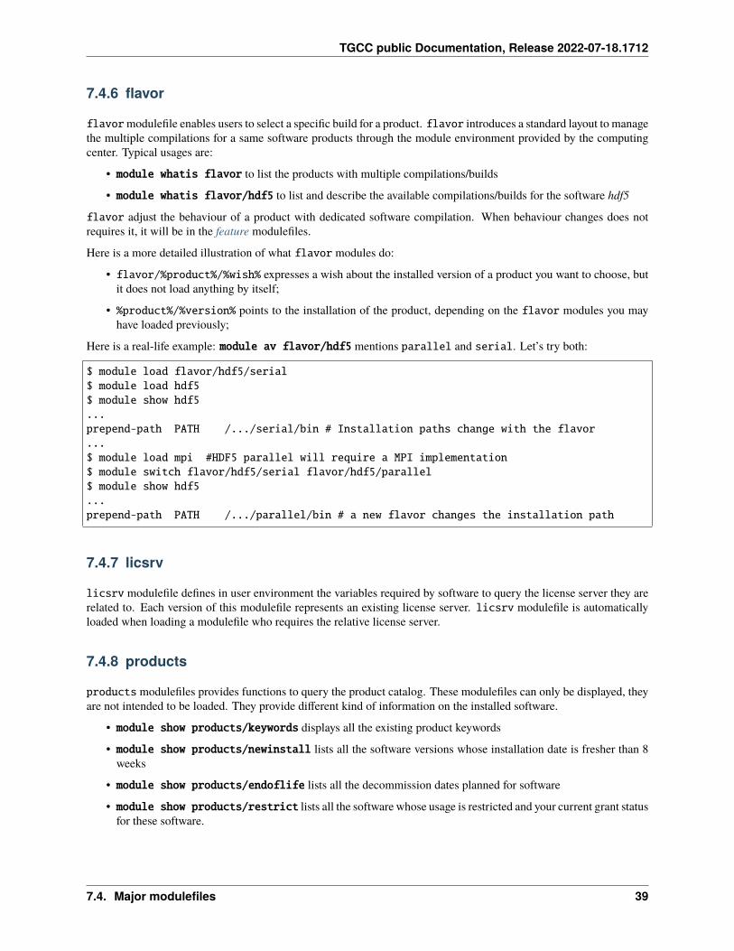
• flavor/%product%/%wish% expresses a wish about the installed version of a product you want to choose, butit does not load anything by itself;
• %product%/%version% points to the installation of the product, depending on the flavor modules you mayhave loaded previously;
Here is a real-life example: module av flavor/hdf5 mentions parallel and serial. Let’s try both:
$ module load flavor/hdf5/serial$ module load hdf5$ module show hdf5...prepend-path PATH /.../serial/bin # Installation paths change with the flavor...$ module load mpi #HDF5 parallel will require a MPI implementation$ module switch flavor/hdf5/serial flavor/hdf5/parallel$ module show hdf5...prepend-path PATH /.../parallel/bin # a new flavor changes the installation path
7.4.7 licsrv
licsrv modulefile defines in user environment the variables required by software to query the license server they arerelated to. Each version of this modulefile represents an existing license server. licsrv modulefile is automaticallyloaded when loading a modulefile who requires the relative license server.
7.4.8 products
products modulefiles provides functions to query the product catalog. These modulefiles can only be displayed, theyare not intended to be loaded. They provide different kind of information on the installed software.
• module show products/keywords displays all the existing product keywords
• module show products/newinstall lists all the software versions whose installation date is fresher than 8weeks
• module show products/endoflife lists all the decommission dates planned for software
• module show products/restrict lists all the software whose usage is restricted and your current grant statusfor these software.
7.4. Major modulefiles 39
TGCC public Documentation, Release 2022-07-18.1712
7.5 Extend your environment with modulefiles
Computing center staff provides you regular HPC software you can access through the module environment. You mayneed to extend this regular environment with your own product installations or various setups. This section describeshow to enable your environment extensions within the module environment.
7.5.1 Using the extenv modulefile
extenv modulefile enables users to extend the environment provided by the computing center staff with extra environ-ment managed within its own home directory or within a shared/application space home directory. extenv introducesa standard layout to manage your software products through the module environment provided by the computing center.This modulefile enables to define a common environment for all users of a given shared space.
A version for extenv modulefile exists for each shared space known in the computing center, named in accordanceto the shared space name, and for the user personal space, named own. You can only view and access versions of theextenv modulefile that correspond to spaces you can access. Multiple versions of the extenv module can be loadedat the same time.
Loading the extenv modulefile will:
• Set environment variables defining the path to shared products and modulefiles (SHSPACE_PRODUCTSHOME,SHSPACE_MODULEFILES, SHSPACE_MODULESHOME)
• Execute a module initialization script
• Add shared modulefiles to the list of available modulefiles
The environment extension mechanisms of extenv requires the use of specific paths. Products installed for the sharedspace named shspace should be installed in $SHSPACE_PRODUCTSHOME and the corresponding modulefiles should bein $SHSPACE_MODULEFILES.
Initialization file
If a file named init is found in the path defined by $SHSPACE_MODULESHOME, then each time the extenv/shspacemodule is loaded, this initialization file will be executed as TCL code. This may be useful if you want to define othercommon environment variables or add prerequisites on modules to be used by the community.
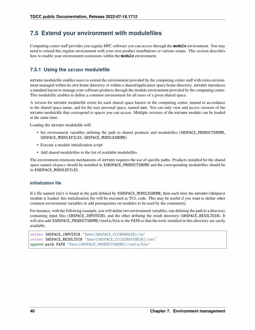
For instance, with the following example, you will define two environment variables, one defining the path to a directorycontaining input files (SHSPACE_INPUTDIR), and the other defining the result directory (SHSPACE_RESULTDIR). Itwill also add $SHSPACE_PRODUCTSHOME/tools/bin to the PATH so that the tools installed in this directory are easilyavailable.
setenv SHSPACE_INPUTDIR "$env(SHSPACE_CCCWORKDIR)/in"setenv SHSPACE_RESULTDIR "$env(SHSPACE_CCCSCRATCHDIR)/res"append-path PATH "$env(SHSPACE_PRODUCTSHOME)/tools/bin"
40 Chapter 7. Environment management
TGCC public Documentation, Release 2022-07-18.1712
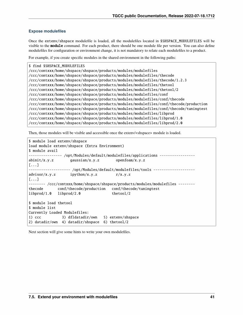
Expose modulefiles
Once the extenv/shspace modulefile is loaded, all the modulefiles located in $SHSPACE_MODULEFILES will bevisible to the module command. For each product, there should be one module file per version. You can also definemodulefiles for configuration or environment change, it is not mandatory to relate each modulefiles to a product.
For example, if you create specific modules in the shared environment in the following paths:
$ find $SHSPACE_MODULEFILES/ccc/contxxx/home/shspace/shspace/products/modules/modulefiles/ccc/contxxx/home/shspace/shspace/products/modules/modulefiles/thecode/ccc/contxxx/home/shspace/shspace/products/modules/modulefiles/thecode/1.2.3/ccc/contxxx/home/shspace/shspace/products/modules/modulefiles/thetool/ccc/contxxx/home/shspace/shspace/products/modules/modulefiles/thetool/2/ccc/contxxx/home/shspace/shspace/products/modules/modulefiles/conf/ccc/contxxx/home/shspace/shspace/products/modules/modulefiles/conf/thecode/ccc/contxxx/home/shspace/shspace/products/modules/modulefiles/conf/thecode/production/ccc/contxxx/home/shspace/shspace/products/modules/modulefiles/conf/thecode/tuningtest/ccc/contxxx/home/shspace/shspace/products/modules/modulefiles/libprod/ccc/contxxx/home/shspace/shspace/products/modules/modulefiles/libprod/1.0/ccc/contxxx/home/shspace/shspace/products/modules/modulefiles/libprod/2.0
Then, those modules will be visible and accessible once the extenv/<shspace> module is loaded.
$ module load extenv/shspaceload module extenv/shspace (Extra Environment)$ module avail---------------- /opt/Modules/default/modulefiles/applications -----------------abinit/x.y.z gaussian/x.y.z openfoam/x.y.z[...]-------------------- /opt/Modules/default/modulefiles/tools --------------------advisor/x.y.z ipython/x.y.z r/x.y.z[...]-------- /ccc/contxxx/home/shspace/shspace/products/modules/modulefiles --------thecode conf/thecode/production conf/thecode/tuningtestlibprod/1.0 libprod/2.0 thetool/2
$ module load thetool$ module listCurrently Loaded Modulefiles:1) ccc 3) dfldatadir/own 5) extenv/shspace2) datadir/own 4) datadir/shspace 6) thetool/2
Next section will give some hints to write your own modulefiles.
7.5. Extend your environment with modulefiles 41
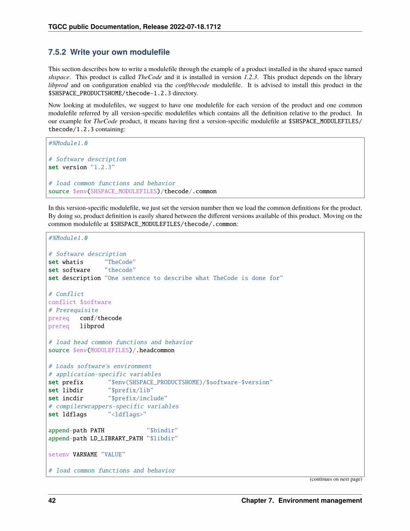
TGCC public Documentation, Release 2022-07-18.1712
7.5.2 Write your own modulefile
This section describes how to write a modulefile through the example of a product installed in the shared space namedshspace. This product is called TheCode and it is installed in version 1.2.3. This product depends on the librarylibprod and on configuration enabled via the conf/thecode modulefile. It is advised to install this product in the$SHSPACE_PRODUCTSHOME/thecode-1.2.3 directory.
Now looking at modulefiles, we suggest to have one modulefile for each version of the product and one commonmodulefile referred by all version-specific modulefiles which contains all the definition relative to the product. Inour example for TheCode product, it means having first a version-specific modulefile at $SHSPACE_MODULEFILES/thecode/1.2.3 containing:
#%Module1.0
# Software descriptionset version "1.2.3"
# load common functions and behaviorsource $env(SHSPACE_MODULEFILES)/thecode/.common
In this version-specific modulefile, we just set the version number then we load the common definitions for the product.By doing so, product definition is easily shared between the different versions available of this product. Moving on thecommon modulefile at $SHSPACE_MODULEFILES/thecode/.common:
#%Module1.0
# Software descriptionset whatis "TheCode"set software "thecode"set description "One sentence to describe what TheCode is done for"
# Conflictconflict $software# Prerequisiteprereq conf/thecodeprereq libprod
# load head common functions and behaviorsource $env(MODULEFILES)/.headcommon
# Loads software's environment# application-specific variablesset prefix "$env(SHSPACE_PRODUCTSHOME)/$software-$version"set libdir "$prefix/lib"set incdir "$prefix/include"# compilerwrappers-specific variablesset ldflags "<ldflags>"
append-path PATH "$bindir"append-path LD_LIBRARY_PATH "$libdir"
setenv VARNAME "VALUE"
# load common functions and behavior(continues on next page)
42 Chapter 7. Environment management
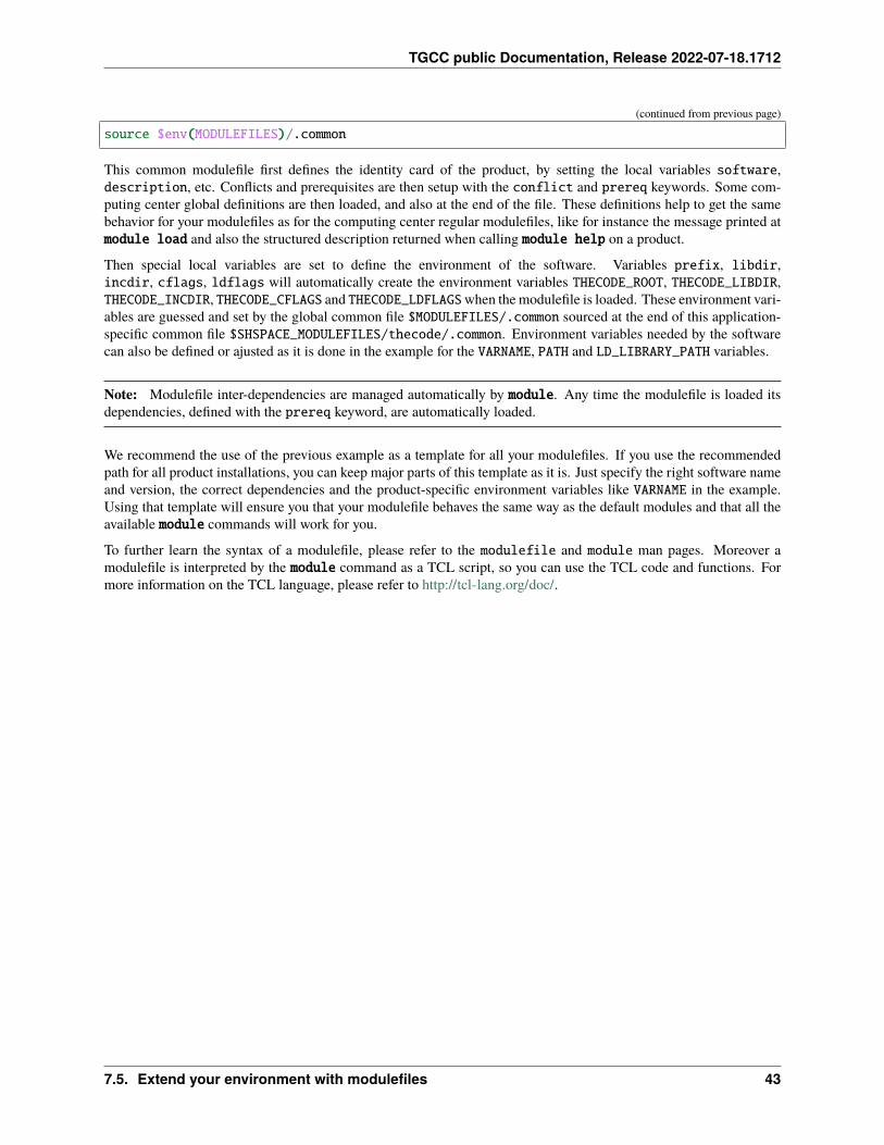
TGCC public Documentation, Release 2022-07-18.1712
(continued from previous page)
source $env(MODULEFILES)/.common
This common modulefile first defines the identity card of the product, by setting the local variables software,description, etc. Conflicts and prerequisites are then setup with the conflict and prereq keywords. Some com-puting center global definitions are then loaded, and also at the end of the file. These definitions help to get the samebehavior for your modulefiles as for the computing center regular modulefiles, like for instance the message printed atmodule load and also the structured description returned when calling module help on a product.
Then special local variables are set to define the environment of the software. Variables prefix, libdir,incdir, cflags, ldflags will automatically create the environment variables THECODE_ROOT, THECODE_LIBDIR,THECODE_INCDIR, THECODE_CFLAGS and THECODE_LDFLAGSwhen the modulefile is loaded. These environment vari-ables are guessed and set by the global common file $MODULEFILES/.common sourced at the end of this application-specific common file $SHSPACE_MODULEFILES/thecode/.common. Environment variables needed by the softwarecan also be defined or ajusted as it is done in the example for the VARNAME, PATH and LD_LIBRARY_PATH variables.
Note: Modulefile inter-dependencies are managed automatically by module. Any time the modulefile is loaded itsdependencies, defined with the prereq keyword, are automatically loaded.
We recommend the use of the previous example as a template for all your modulefiles. If you use the recommendedpath for all product installations, you can keep major parts of this template as it is. Just specify the right software nameand version, the correct dependencies and the product-specific environment variables like VARNAME in the example.Using that template will ensure you that your modulefile behaves the same way as the default modules and that all theavailable module commands will work for you.
To further learn the syntax of a modulefile, please refer to the modulefile and module man pages. Moreover amodulefile is interpreted by the module command as a TCL script, so you can use the TCL code and functions. Formore information on the TCL language, please refer to http://tcl-lang.org/doc/.
7.5. Extend your environment with modulefiles 43
TGCC public Documentation, Release 2022-07-18.1712
44 Chapter 7. Environment management
CHAPTER
EIGHT
SOFTWARES
This section presents the various kinds of software products (binaries, libraries, scripts and tools) available on thecenter. It is organized as follows. After generally explaining the different kinds of software on the center, we willfocus on specific cases (restricted and purchased products). Finally, we will talk about the software life cycle, from theinstallation request to the product removal.
8.1 Generalities on software
Lots of tools and products are available on the supercomputer. A distinction is made between the OS and CCC software.
8.1.1 OS software
They are software products provided by the operating system. They are installed by packages (rpm) and are locallystored on each node.
All common Linux software products enter in this category, such as:
• shells (bash, tcsh),
• common scripting tools (cat, sed, awk, . . . )
• editors (vi, emacs, gedit, . . . ),
• minimal installations of common scripting language (perl, python).
Updates occur during maintenance or during production only if they do not impact the operating system of the node.
8.1.2 CCC software
CCC software products are the third-party dedicated tools or dedicated compilations. They are shared by all centernodes and are installed by TGCC-CCRT dedicated service(s) during production. We prefer the term CCC softwareproducts over center software which is ambiguous.
Contrary to the OS software products, CCC software products are not within the standard operating system paths forbinaries or libraries (eg. /usr/bin or /usr/lib64).
Each product is installed in a dedicated directory and requires an update of environment variables like and before use.These environment updates are handled by the module tool detailed in the Environment management section.
Updates occur during production as they do not interrupt nor interfere with the operating system installation.
45
TGCC public Documentation, Release 2022-07-18.1712
8.1.3 Software and module
A CCC software product requires an environment update before use. The module command is the tool for it, so amodule exists for each CCC software product.
An OS software product is usually not referred to by a module, except when:
• it is usually the case in other computing centers (ex: tcl)
• there is a CCC software version of it (ex: valgrind): it helps to avoid conflicts between the OS and CCCinstallation.
Products referenced by module have been organized into categories:
• applications: simulation products
• environment: defines the user/group environment
• tools: development tools
• graphics: visualization or image manipulation tools
• parallel: parallel execution software such as MPI
• libraries: third-party libraries
• compilers: the various compilers
A domain-oriented view is provided by module search <keyword>. To list the valid keywords use:
module help products/keywords
8.1.4 Software toolchains
Warning: Please refer to internal technical documentation to get information about available toolchains.
This approach provides a variety of compilation / runtime environments to users with consistency across products. Toconsult the list of available builds for a given product, type module help <product>.
The selection between toolchains is made with two modules flavor/buildcompiler/<compiler>/<version> andflavor/buildmpi/<mpi>/<version>. It allows you to change the toolchain used for any loaded product regardlessof the Intel compiler and MPI implementation used at runtime, which is determined by your current intel and mpimodules loaded.
More information on the flavor mechanism can be found on the dedicated section.
The module flavor/buildcompiler/<compiler>/<version> lets you choose the version of the Intel compilerwhereas the module flavor/buildmpi/<mpi>/<version> lets you choose the MPI implementation and version.
46 Chapter 8. Softwares
TGCC public Documentation, Release 2022-07-18.1712
8.2 Specific software
The center has specific rules for restricted products and purchased products.
8.2.1 Restricted software products
A restricted product is referenced by module, but its access is restricted to a specific Unix group. Although the reasonsmay vary, this usually comes from a license requirement.
For example, a licensed product may restrict its usage to academic purposes, or the purchased license is an academicone.
Warning: Please refer to internal technical documentation to get information about this subject.
Installation request and restricted products
Warning: Please refer to internal technical documentation to get information about this subject.
8.2.2 Products with purchased license
Some products (such as Intel compilers) require a license server. We refer to them as licensed products.
Module and licensed products
Here are several adaptations of module for licensed products:
• A licensed product module depends on a license module to find its license server.
• Although the license module is not shown at load time, a module list can display it.
• license module are named licsrv/<server> and are listed by:
module avail licsrv
Installation request and purchased products
While requesting the installation of a purchased product, you may:
• have a license not requiring a dedicated server,
• have the license and want to restrict its usage to a group of people (because you only have a few tokens),
• have a global license (limited in time),
• have no license and ask for the center to purchase it.
The two first cases are handled by defining it as a restricted product.
The last case must be clearly justified. If so, you must at least:
• estimate the number of user,
• specify its application domain,
8.2. Specific software 47
TGCC public Documentation, Release 2022-07-18.1712
• tell us if you need the academic or the commercial license,
• and tell us if you need a global license and/or how many tokens are necessary.
Please note that, even if such installation follows the usual validation process, you may have additional delays, namely:
• if you need a non-FlexNet dedicated license server,
• if you need to generate some license server identification (done by us and filtered for security reasons) beforegetting the license.
8.3 Product Life cycle
Here are the phases of a software product life cycle, explained chronologically from its installation request to its dep-recation and removal.
8.3.1 Installation request
New products and/or product update(s) can be requested by mail to the TGCC-CCRT hotline.
Requests are usually accepted if:
• the product is the last stable version,
• the product is useful to many users,
• the product has no license issue.
There are also special cases, namely:
• an installation for a group of persons is not possible since these persons are not part of the same user container,
• or the product access should be restricted (see Installation request and restricted products),
• or the product requires a license server (see Installation request and purchased products).
8.3.2 Installation phase
If the installation request is approved, we will proceed to the installation itself:
• for an OS software product, it should be done at the next maintenance (or before if this is deemed safe).
• and for an CCC software product, it should take several days.
Note: Those are estimated installation times. If technical difficulties occur the installation may take longer (example:licensed products)
Newly installed CCC software maybe listed with:
module show products/newinstall
48 Chapter 8. Softwares
TGCC public Documentation, Release 2022-07-18.1712
8.3.3 Production phase
During the production, the software product should be operational. If you detect an issue, a bug or a missing feature,please report it to the TGCC-CCRT hotline.
8.3.4 End-of-life and removal
An OS software product is considered obsolete when either the distribution considers it as such or when an update hasbeen planned for the next maintenance.
For CCC software products, we try to respect the following rules. For each CCC software product, the center favorsversions with the least bugs, the most features and the best performances. Hence the last stable version of a product isvery welcome (new features, better performances and bug corrections). So when a new version of a product is installed,previous versions may become obsolete. To be more specific, we will only keep:
• the latest version,
• its last known stable(s) version(s) (for reference purpose),
• and the version(s) before retro-compatibility issues (mainly API break).
As retro-compatibility issues may be unknown, removal of obsolete products are scheduled: they have reached their“end-of-life”.
module has been extended accordingly:
• load, help or show actions will display the following message for obsolete products:
End-of-life disclaimer:<product>/<version> is deprecated and has been decommissioned on** YYYY-MM-DD **. You are advised to use the default version of thesoftware instead of this specific version. Please contact support ifyou encounter issue with software default version.
• To list the products tagged as end-of-life, with their due date, type:
module show products/endoflife
At the due date, the CCC product in end-of-life state is uninstalled unless a user has given a valid reason to keep it.Hence, if the removal of a deprecated product is an issue for you, please contact the TGCC-CCRT hotline as soon aspossible.
8.3. Product Life cycle 49
TGCC public Documentation, Release 2022-07-18.1712
50 Chapter 8. Softwares
CHAPTER
NINE
JOB SUBMISSION
Computing nodes are shared between all the users of the computing center. A job scheduler manages the access tothe global resources and allows users to book the resources they need for their computation. Job submission, resourceallocation and job launch are handled by the batch scheduler called SLURM. An abstraction layer called Bridge isprovided to give uniform command-line tools and more integrated ways to access batch scheduling systems.
To submit a batch job, you first have to write a shell script containing:
• a set of directives to tell which resources your job needs.
• instructions to execute your code.
You can launch the job by submitting its script to the batch scheduler. It will enter a batch queue. When resourcesbecome available, the job is launched over its allocated nodes. Jobs can be monitored.
9.1 Scheduling policy
Jobs are submitted to the supercomputer resource manager which will decide how to schedule them. There are hundredsof jobs submitted daily and the order in which they are launched depends on several parameters.
Jobs are sorted by priority. The priority is an integer value initially assigned to the job when it is submitted. The jobwith the highest priority will start first as soon as enough resources are available. Sometimes, a job with a lower prioritymay start first but only if it does not delay any job with a higher priority. This mechanism is called backfill schedulingand jobs can easily be backfilled if they require few computing resources and have a small time limit.
Here are the 3 components that are added to obtain the priority. They are listed below in order of importance:
• The Quality of Service (QoS): The QoS component is a constant value associated to the QoS chosen during thesubmission. Its value depends on the priority factor given by the ccc_mqinfo command. This is the componentthat has the most influence on the overall value of the priority. Also, an usage limit can be set to prevent jobsfrom running as long as the project is not under a certain consumption. See Qos for more information.
• The project’s fair-share: The fair-share component reflects the ratio between the total share of allocated hoursand the amount of hours consumed for the chosen project. The fair-share value will be high if the project isunder-consuming its allocated hours whereas it will be low if the project is over-consuming its allocated hours.A half-life decay is applied to the computation of the fair-share with a half life period of 14 days. That way, anover-consumption or under-consumption of hours will have a decreasing impact on new jobs submissions. After2 months, the negative impact of an over-consumption is almost insignificant.
• The job’s age: The age component depends on the time spent in a pending state while waiting for resources. Itsvalue is incremented regularly for 7 days. After this delay, it will not increase anymore.
In order to reduce the waiting time as much as possible, try to:
• Use your computing hours evenly throughout your project duration. It will increase your fair-share value, thusincrease the priority of your jobs.
51
TGCC public Documentation, Release 2022-07-18.1712
• For small jobs, specify a time limit as close as possible to the real duration of the job instead of leaving defaulttime limit of 2 hours. That way you are more likely to benefit from the backfill scheduling mechanism.
• Since the default time limit is 2 hours for all jobs, try to specify a time limit as close as possible to the realduration of your job. That way you are more likely to benefit from the backfill scheduling mechanism.
9.2 Choosing the file systems
Your job submissions can use the -m option to specify the file systems compute nodes will need for execution. Thisavoids job suspensions, if an unused file system becomes unavailable.
example: ccc_msub -m scratch,store will run even if the WORK file system is unavailable. You canchoose the following file systems: scratch, work and store.
Warning: On Irene, your job submissions MUST use the -m option. Failing to provide the -m option will actuallyprevent your compute nodes from using any of scratch, work or store.
9.3 Submission scripts
9.3.1 ccc_msub
ccc_msub <script> is the command used to submit your batch job to the resource manager. The options passed toccc_msub will determine the number of cores allocated to the job.
There are two ways of passing arguments to ccc_msub.
• Use the #MSUB keyword in the submission script. All the lines beginning with #MSUB will be parsed and thecorresponding parameters will be taken into account by the batch manager.
• Use command line arguments. If the same argument is specified in the command line and the submission script,the command line argument will take precedence.
Note that you cannot pass arguments to the submission script when launching with ccc_msub.
For a short documentation and list of available options, see the help message:
$ ccc_msub -h
Basic options
• -o output_file: standard output file (special character %I will be replaced by the job ID)
• -e error_file: standard error file (special character %I will be replaced by the job ID)
All the output and error messages generated by the job are redirected to the log files specified with -o and -e. If youwant all output to be redirected in one single file, just set the same name for -o and -e.
• -r reqname: job name
• -A projid: project/account name
• -m filesystem: file system required by the job. If another file system is unavailable, the job will not beimpacted. Without the option, the job is considered to use every file system
52 Chapter 9. Job submission
TGCC public Documentation, Release 2022-07-18.1712
example: ccc_msub -m scratch,storewill run even if the WORK file system is unavailable. You can choosethe following file systems: scratch, work and store.
• -@ mailopts: mail options following the pattern mailaddr[:begin|end|requeue]
example: ccc_msub -@ [email protected]:begin,end will send a mail to jdoe at the beginning and the end ofthe job default behavior depends of the underlying batch system
Partitions
The compute nodes are gathered in partitions according to their hardware characteristics (CPU architecture, amountof RAM, presence of GPU, etc). A partition is a set of identical nodes that can be targeted to host one or severaljobs. Choosing the right partition for a job depends on code prerequisites in term of hardware resources. For example,executing a code designed to be GPU accelerated requires a partition with GPU nodes.
The partition is specified with the -q option. This option is mandatory while submitting.
The ccc_mpinfo command lists the available partitions for the current supercomputer. For each partition, it willdisplay the number of available cores and nodes but also give some hardware specifications of the nodes composingthe partition. For more information, see the Supercomputer architecture section.
Note:
• This choice is exclusive: your job can only be submitted on one of those architectures at a time.
• Job priority and limits are not related to the partition but to the QoS (Quality of Service) parameter (option -Q).QoS is the main component of job priority.
• Depending on the allocation granted to your project, you may not have access to all the partitions. You can checkon which partition(s) your project has allocated hours thanks to the command ccc_myproject.
Resources
There are several options that will influence the number of cores that will be allocated for the job.
• -n: number of tasks that will be used in parallel mode (default=1)
• -c: number of cores per parallel task to allocate (default=1)
If the -c parameter is not specified, the number of cores allocated is equal to the number of parallel tasks requestedwith -n. So specifying -n is enough for most of the basic jobs. The -c option is useful when each MPI processlaunched needs more resources than just one core. It can be either to require more cpu power or more memory:
– For hybrid MPI/OpenMP jobs, each MPI process will need several cores in order to spawn its OpenMPthreads. In that case, usually, the -c option is equal to the number passed to OMP_NUM_THREADS
– For jobs requiring a lot of memory, each MPI process may need more than the 4 GB it is granted by default.In that case, the amount of memory may be multiplied by allocating more cores for each process. Forexample, by specifying -c 2, each process will be able to use the memory of 2 cores: 8GB.
• -N: number of nodes to allocate for parallel usage (default is chosen by the underlying system)
The -N option is not necessary in most of the cases. The number of nodes to use is inferred by the number ofcores requested and the number of cores per node of the partition used.
• -x: request for exclusive usage of allocated nodes
The -x options forces the allocation of a whole node, even if only a couple of cores were requested. This is thedefault configuration for jobs requiring more than 128 cores.
9.3. Submission scripts 53
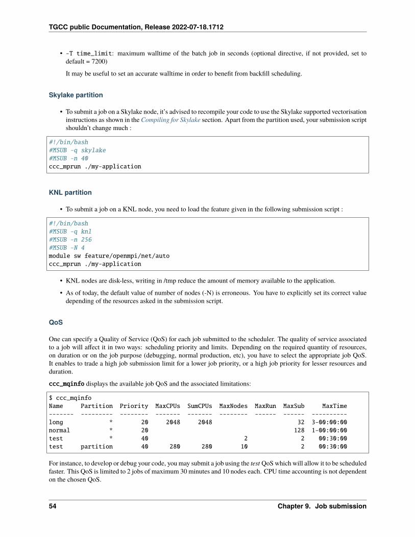
TGCC public Documentation, Release 2022-07-18.1712
• -T time_limit: maximum walltime of the batch job in seconds (optional directive, if not provided, set todefault = 7200)
It may be useful to set an accurate walltime in order to benefit from backfill scheduling.
Skylake partition
• To submit a job on a Skylake node, it’s advised to recompile your code to use the Skylake supported vectorisationinstructions as shown in the Compiling for Skylake section. Apart from the partition used, your submission scriptshouldn’t change much :
#!/bin/bash#MSUB -q skylake#MSUB -n 40ccc_mprun ./my-application
KNL partition
• To submit a job on a KNL node, you need to load the feature given in the following submission script :
#!/bin/bash#MSUB -q knl#MSUB -n 256#MSUB -N 4module sw feature/openmpi/net/autoccc_mprun ./my-application
• KNL nodes are disk-less, writing in /tmp reduce the amount of memory available to the application.
• As of today, the default value of number of nodes (-N) is erroneous. You have to explicitly set its correct valuedepending of the resources asked in the submission script.
QoS
One can specify a Quality of Service (QoS) for each job submitted to the scheduler. The quality of service associatedto a job will affect it in two ways: scheduling priority and limits. Depending on the required quantity of resources,on duration or on the job purpose (debugging, normal production, etc), you have to select the appropriate job QoS.It enables to trade a high job submission limit for a lower job priority, or a high job priority for lesser resources andduration.
ccc_mqinfo displays the available job QoS and the associated limitations:
$ ccc_mqinfoName Partition Priority MaxCPUs SumCPUs MaxNodes MaxRun MaxSub MaxTime------- --------- -------- ------- ------- -------- ------ ------ ----------long * 20 2048 2048 32 3-00:00:00normal * 20 128 1-00:00:00test * 40 2 2 00:30:00test partition 40 280 280 10 2 00:30:00
For instance, to develop or debug your code, you may submit a job using the test QoS which will allow it to be scheduledfaster. This QoS is limited to 2 jobs of maximum 30 minutes and 10 nodes each. CPU time accounting is not dependenton the chosen QoS.
54 Chapter 9. Job submission
TGCC public Documentation, Release 2022-07-18.1712
To specify a QoS, you can use the -Q option of command-line or add #MSUB -Q <qosname> directive to your submis-sion script. If no QoS is mentioned, default QoS normal will be used.
An usage limit can be set to manage hours consumption within a project. The usage limit can be set to high, mediumor low with the option #MSUB -U <limit>.
• A job submitted with -U high priority will be scheduled normally as described in Scheduling policy. This isthe default behavior if no usage limit is specified.
• A job submitted with -U medium will only be scheduled if the current project consumption is less than 20% overthe suggested use at this time.
• A job submitted with -U low will only be scheduled if the current project consumption is more than 20% underthe suggested use at this time.
Medium and low priority jobs may stay pending even if all the resources are free. It allows to prevent non importantjobs from over consuming project hours and thus lower the default priority of future important jobs.
Creating a virtual cluster
It’s possible to use the ccc_msub -z <pcocc_template> command to submit a job on a virtual cluster created withpcocc VMs. More information on usage can be found in the Virtualization Bridge plugin section.
Dependencies between jobs
Note: The following methods are equivalent concerning the priorities of dependent jobs. See the Scheduling policysection for more details.
The command offers two options to prevent some jobs from running at the same time. Those options are -w and -a:
• The option -w makes jobs with the same submission name (specified with -r) run in the order they were sub-mitted. For example, all jobs with the following options will not run at the same time.
#MSUB -r SAME_NAME#MSUB -w
• The option -a indicates that a job depends on another (already submitted) job. Use it with the id of the existingjob.
ccc_msub -a <existing_job> script.sh
• One can write multi step jobs that run sequentially by submitting the next job at the end of the current script.Here are some example scripts:
JOB_A.sh:
#!/bin/bash#MSUB -r JOB_A#MSUB -n 32#MSUB -q <partition>ccc_mprun ./a.outccc_msub JOB_B.sh
JOB_B.sh:
9.3. Submission scripts 55
TGCC public Documentation, Release 2022-07-18.1712
#!/bin/bash#MSUB -r JOB_B#MSUB -n 16#MSUB -q <partition>ccc_mprun ./b.outccc_msub JOB_C.sh
JOB_C.sh:
#!/bin/bash#MSUB -r JOB_C#MSUB -n 8#MSUB -q <partition>ccc_mprun ./c.out
Then, only JOB_A.sh has to be submitted. When it finishes, the script submits JOB_B.sh, etc. . .
Note: If a job is killed or if it reaches its time limit, all the jobs are removed and the last ccc_msub may not belaunched. To avoid this, you can use the ccc_tremain from libccc_user or use the #MSUB -w directive as describedabove.
Environment variables
When a job is submitted, some environment variables are set. Those variables may be used only within the job script.
• BRIDGE_MSUB_JOBID: batch id of the running job.
• BRIDGE_MSUB_MAXTIME: timelimit in seconds of the job.
• BRIDGE_MSUB_PWD: working directory. Usually the directory in which the job was submitted.
• BRIDGE_MSUB_NPROC: number of requested processes
• BRIDGE_MSUB_NCORE: number of requested cores per process
• BRIDGE_MSUB_REQNAME: job name
Note: You cannot use those variables as input arguments to ccc_msub. You cannot use them with the #MSUB headers.
9.3.2 ccc_mprun
ccc_mprun command allows to launch parallel jobs over nodes allocated by resources manager. So inside a submissionscript, a parallel code will be launched with the following command:
ccc_mprun ./a.out
By default, ccc_mprun takes information (number of nodes, number of processors, etc) from the resources manager tolaunch the job. You can customize its behavior with the command line options. Type ccc_mprun -h for an up-to-dateand complete documentation.
Here are some basic options ccc_mprun:
• -n nproc: number of tasks to run
56 Chapter 9. Job submission
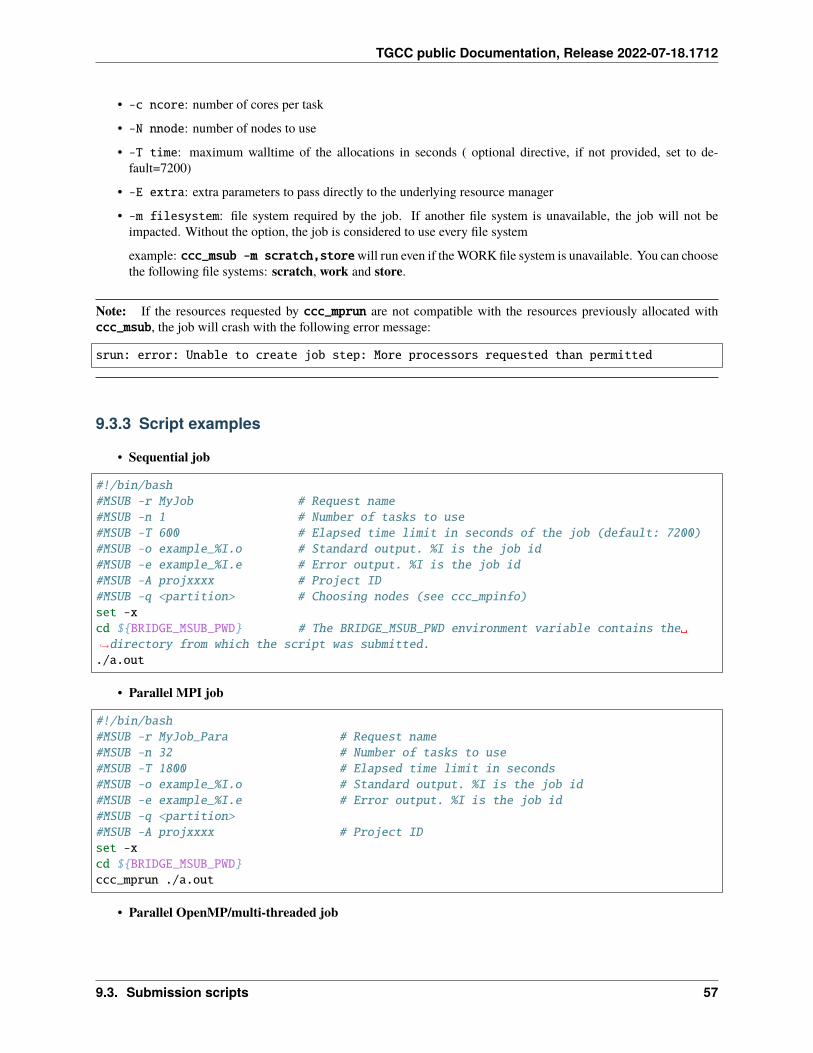
TGCC public Documentation, Release 2022-07-18.1712
• -c ncore: number of cores per task
• -N nnode: number of nodes to use
• -T time: maximum walltime of the allocations in seconds ( optional directive, if not provided, set to de-fault=7200)
• -E extra: extra parameters to pass directly to the underlying resource manager
• -m filesystem: file system required by the job. If another file system is unavailable, the job will not beimpacted. Without the option, the job is considered to use every file system
example: ccc_msub -m scratch,storewill run even if the WORK file system is unavailable. You can choosethe following file systems: scratch, work and store.
Note: If the resources requested by ccc_mprun are not compatible with the resources previously allocated withccc_msub, the job will crash with the following error message:
srun: error: Unable to create job step: More processors requested than permitted
9.3.3 Script examples
• Sequential job
#!/bin/bash#MSUB -r MyJob # Request name#MSUB -n 1 # Number of tasks to use#MSUB -T 600 # Elapsed time limit in seconds of the job (default: 7200)#MSUB -o example_%I.o # Standard output. %I is the job id#MSUB -e example_%I.e # Error output. %I is the job id#MSUB -A projxxxx # Project ID#MSUB -q <partition> # Choosing nodes (see ccc_mpinfo)set -xcd ${BRIDGE_MSUB_PWD} # The BRIDGE_MSUB_PWD environment variable contains the␣→˓directory from which the script was submitted../a.out
• Parallel MPI job
#!/bin/bash#MSUB -r MyJob_Para # Request name#MSUB -n 32 # Number of tasks to use#MSUB -T 1800 # Elapsed time limit in seconds#MSUB -o example_%I.o # Standard output. %I is the job id#MSUB -e example_%I.e # Error output. %I is the job id#MSUB -q <partition>#MSUB -A projxxxx # Project IDset -xcd ${BRIDGE_MSUB_PWD}ccc_mprun ./a.out
• Parallel OpenMP/multi-threaded job
9.3. Submission scripts 57
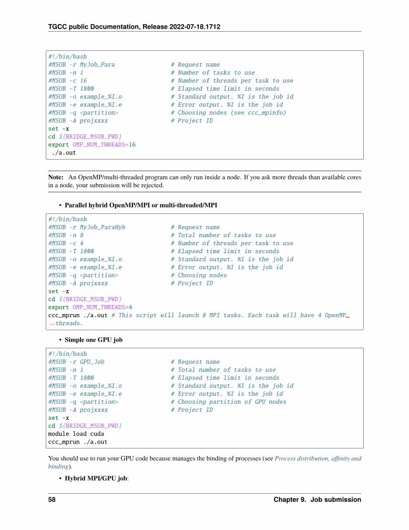
TGCC public Documentation, Release 2022-07-18.1712
#!/bin/bash#MSUB -r MyJob_Para # Request name#MSUB -n 1 # Number of tasks to use#MSUB -c 16 # Number of threads per task to use#MSUB -T 1800 # Elapsed time limit in seconds#MSUB -o example_%I.o # Standard output. %I is the job id#MSUB -e example_%I.e # Error output. %I is the job id#MSUB -q <partition> # Choosing nodes (see ccc_mpinfo)#MSUB -A projxxxx # Project IDset -xcd ${BRIDGE_MSUB_PWD}export OMP_NUM_THREADS=16./a.out
Note: An OpenMP/multi-threaded program can only run inside a node. If you ask more threads than available coresin a node, your submission will be rejected.
• Parallel hybrid OpenMP/MPI or multi-threaded/MPI
#!/bin/bash#MSUB -r MyJob_ParaHyb # Request name#MSUB -n 8 # Total number of tasks to use#MSUB -c 4 # Number of threads per task to use#MSUB -T 1800 # Elapsed time limit in seconds#MSUB -o example_%I.o # Standard output. %I is the job id#MSUB -e example_%I.e # Error output. %I is the job id#MSUB -q <partition> # Choosing nodes#MSUB -A projxxxx # Project IDset -xcd ${BRIDGE_MSUB_PWD}export OMP_NUM_THREADS=4ccc_mprun ./a.out # This script will launch 8 MPI tasks. Each task will have 4 OpenMP␣→˓threads.
• Simple one GPU job
#!/bin/bash#MSUB -r GPU_Job # Request name#MSUB -n 1 # Total number of tasks to use#MSUB -T 1800 # Elapsed time limit in seconds#MSUB -o example_%I.o # Standard output. %I is the job id#MSUB -e example_%I.e # Error output. %I is the job id#MSUB -q <partition> # Choosing partition of GPU nodes#MSUB -A projxxxx # Project IDset -xcd ${BRIDGE_MSUB_PWD}module load cudaccc_mprun ./a.out
You should use to run your GPU code because manages the binding of processes (see Process distribution, affinity andbinding).
• Hybrid MPI/GPU job:
58 Chapter 9. Job submission
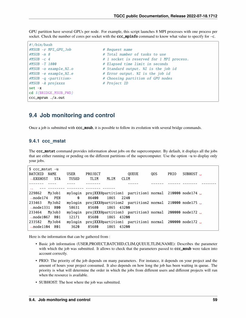
TGCC public Documentation, Release 2022-07-18.1712
GPU partition have several GPUs per node. For example, this script launches 8 MPI processes with one process persocket. Check the number of cores per socket with the ccc_mpinfo command to know what value to specify for -c.
#!/bin/bash#MSUB -r MPI_GPU_Job # Request name#MSUB -n 8 # Total number of tasks to use#MSUB -c 4 # 1 socket is reserved for 1 MPI process.#MSUB -T 1800 # Elapsed time limit in seconds#MSUB -o example_%I.o # Standard output. %I is the job id#MSUB -e example_%I.e # Error output. %I is the job id#MSUB -q <partition> # Choosing partition of GPU nodes#MSUB -A projxxxx # Project IDset -xcd ${BRIDGE_MSUB_PWD}ccc_mprun ./a.out
9.4 Job monitoring and control
Once a job is submitted with ccc_msub, it is possible to follow its evolution with several bridge commands.
9.4.1 ccc_mstat
The ccc_mstat command provides information about jobs on the supercomputer. By default, it displays all the jobsthat are either running or pending on the different partitions of the supercomputer. Use the option -u to display onlyyour jobs.
$ ccc_mstat -uBATCHID NAME USER PROJECT QUEUE QOS PRIO SUBHOST ␣→˓EXEHOST STA TUSED TLIM MLIM CLIM------- ---- ---- ------- ----- ------ ------ ------- -------→˓ --- -------- -------- ------- ------229862 MyJob1 mylogin projXXX@partition1 partition1 normal 210000 node174 ␣→˓node174 PEN 0 86400 1865 2240233463 MyJob2 mylogin projXXX@partition2 partition2 normal 210000 node175 ␣→˓node1331 R00 58631 85680 1865 43200233464 MyJob3 mylogin projXXX@partition3 partition3 normal 200000 node172 ␣→˓node1067 R01 12171 85680 1865 43200233582 MyJob4 mylogin projXXX@partition1 partition1 normal 200000 node172 ␣→˓node1104 R01 3620 85680 1865 43200
Here is the information that can be gathered from :
• Basic job information (USER,PROJECT,BATCHID,CLIM,QUEUE,TLIM,NAME): Describes the parameterwith which the job was submitted. It allows to check that the parameters passed to ccc_msub were taken intoaccount correctly.
• PRIO: The priority of the job depends on many parameters. For instance, it depends on your project and theamount of hours your project consumed. It also depends on how long the job has been waiting in queue. Thepriority is what will determine the order in which the jobs from different users and different projects will runwhen the resource is available.
• SUBHOST: The host where the job was submitted.
9.4. Job monitoring and control 59
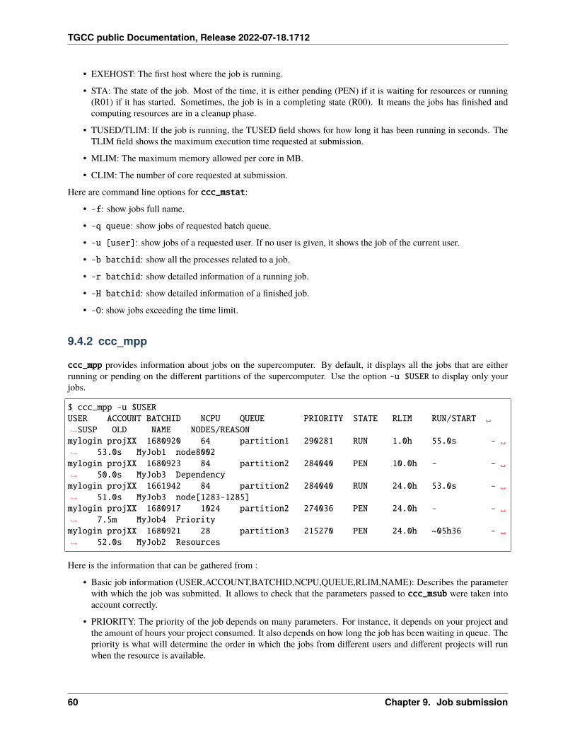
TGCC public Documentation, Release 2022-07-18.1712
• EXEHOST: The first host where the job is running.
• STA: The state of the job. Most of the time, it is either pending (PEN) if it is waiting for resources or running(R01) if it has started. Sometimes, the job is in a completing state (R00). It means the jobs has finished andcomputing resources are in a cleanup phase.
• TUSED/TLIM: If the job is running, the TUSED field shows for how long it has been running in seconds. TheTLIM field shows the maximum execution time requested at submission.
• MLIM: The maximum memory allowed per core in MB.
• CLIM: The number of core requested at submission.
Here are command line options for ccc_mstat:
• -f: show jobs full name.
• -q queue: show jobs of requested batch queue.
• -u [user]: show jobs of a requested user. If no user is given, it shows the job of the current user.
• -b batchid: show all the processes related to a job.
• -r batchid: show detailed information of a running job.
• -H batchid: show detailed information of a finished job.
• -O: show jobs exceeding the time limit.
9.4.2 ccc_mpp
ccc_mpp provides information about jobs on the supercomputer. By default, it displays all the jobs that are eitherrunning or pending on the different partitions of the supercomputer. Use the option -u $USER to display only yourjobs.
$ ccc_mpp -u $USERUSER ACCOUNT BATCHID NCPU QUEUE PRIORITY STATE RLIM RUN/START ␣→˓SUSP OLD NAME NODES/REASONmylogin projXX 1680920 64 partition1 290281 RUN 1.0h 55.0s - ␣→˓ 53.0s MyJob1 node8002mylogin projXX 1680923 84 partition2 284040 PEN 10.0h - - ␣→˓ 50.0s MyJob3 Dependencymylogin projXX 1661942 84 partition2 284040 RUN 24.0h 53.0s - ␣→˓ 51.0s MyJob3 node[1283-1285]mylogin projXX 1680917 1024 partition2 274036 PEN 24.0h - - ␣→˓ 7.5m MyJob4 Prioritymylogin projXX 1680921 28 partition3 215270 PEN 24.0h ~05h36 - ␣→˓ 52.0s MyJob2 Resources
Here is the information that can be gathered from :
• Basic job information (USER,ACCOUNT,BATCHID,NCPU,QUEUE,RLIM,NAME): Describes the parameterwith which the job was submitted. It allows to check that the parameters passed to ccc_msub were taken intoaccount correctly.
• PRIORITY: The priority of the job depends on many parameters. For instance, it depends on your project andthe amount of hours your project consumed. It also depends on how long the job has been waiting in queue. Thepriority is what will determine the order in which the jobs from different users and different projects will runwhen the resource is available.
60 Chapter 9. Job submission
TGCC public Documentation, Release 2022-07-18.1712
• STATE: The state of the job. Most of the time, it is either pending (PEN) if it is waiting for resources or running(RUN) if it has started. Sometimes, the job is in a completing state (COMP). It means the jobs has finished andcomputing resources are in a cleanup phase.
• RUN/START: If the job is running, this field shows for how long it has been running. If the job is pending,it sometimes gives an evaluation of the estimated start time. This start time may vary depending on the jobssubmitted by other users.
• SUSP: The time spent in a suspended state. Jobs may be suspended by staff when an issue occur on the super-computer. In that case, running jobs are not flushed but suspended in order to let them continue once the issueis solved.
• OLD: The total amount of time since the job was submitted. It includes the time spent waiting and running.
• NODES/REASON: If the job is running, this gives you the list of nodes used by the job. If it is pending, itgives you the reason. For example, “Dependency” means you submitted the job with a dependency to anotherunfinished job. “Priority” means there are other jobs that have a better priority and yours will start running afterthose. “Resources” means there are not enough cores available at the moment to let the job start. It will haveto wait for some other jobs to end and free their allocated resources. “JobHeldAdmin” means that the currentjob has been held by a user who is not the owner (generaly an admin with the required rights). Please note thatpending jobs with lower priority may display a pending reason not reflecting their current pending state since thebatch scheduler only updates the pending reason of high priority jobs.
Here are command line options for ccc_mpp:
• -r: prints ‘running’ batch jobs
• -s: prints ‘suspended’ batch jobs
• -p: prints ‘pending’ batch jobs
• -q queue: requested batch queue
• -u user: requested user
• -g group: requested group
• -n: prints results without colors
9.4.3 ccc_mpeek
ccc_mpeek gives information about a job while it runs.
$ ccc_mpeek <jobid>
It is particularly useful to check the output of a job while it is running. The default behavior is to display the standardoutput. It is what you would basically find in the .o log file.
Here are command line options for ccc_mpeek:
• -o: prints the standard output
• -e: prints the standard error output
• -s: prints the job submission script
• -t: same as -o in tail -f mode
• -S: print the launched script of the running job
• -d: print the temporary directory of the running job
• -I: print the INFO file of the running job
9.4. Job monitoring and control 61
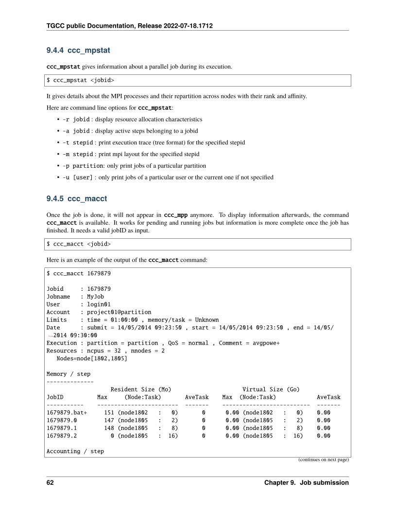
TGCC public Documentation, Release 2022-07-18.1712
9.4.4 ccc_mpstat
ccc_mpstat gives information about a parallel job during its execution.
$ ccc_mpstat <jobid>
It gives details about the MPI processes and their repartition across nodes with their rank and affinity.
Here are command line options for ccc_mpstat:
• -r jobid : display resource allocation characteristics
• -a jobid : display active steps belonging to a jobid
• -t stepid : print execution trace (tree format) for the specified stepid
• -m stepid : print mpi layout for the specified stepid
• -p partition: only print jobs of a particular partition
• -u [user] : only print jobs of a particular user or the current one if not specified
9.4.5 ccc_macct
Once the job is done, it will not appear in ccc_mpp anymore. To display information afterwards, the commandccc_macct is available. It works for pending and running jobs but information is more complete once the job hasfinished. It needs a valid jobID as input.
$ ccc_macct <jobid>
Here is an example of the output of the ccc_macct command:
$ ccc_macct 1679879
Jobid : 1679879Jobname : MyJobUser : login01Account : project01@partitionLimits : time = 01:00:00 , memory/task = UnknownDate : submit = 14/05/2014 09:23:50 , start = 14/05/2014 09:23:50 , end = 14/05/→˓2014 09:30:00Execution : partition = partition , QoS = normal , Comment = avgpowe+Resources : ncpus = 32 , nnodes = 2
Nodes=node[1802,1805]
Memory / step--------------
Resident Size (Mo) Virtual Size (Go)JobID Max (Node:Task) AveTask Max (Node:Task) AveTask----------- ------------------------ ------- -------------------------- -------1679879.bat+ 151 (node1802 : 0) 0 0.00 (node1802 : 0) 0.001679879.0 147 (node1805 : 2) 0 0.00 (node1805 : 2) 0.001679879.1 148 (node1805 : 8) 0 0.00 (node1805 : 8) 0.001679879.2 0 (node1805 : 16) 0 0.00 (node1805 : 16) 0.00
Accounting / step(continues on next page)
62 Chapter 9. Job submission
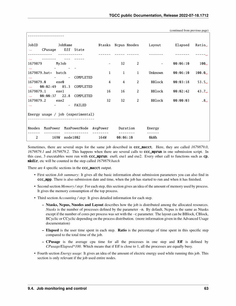
TGCC public Documentation, Release 2022-07-18.1712
(continued from previous page)
------------------
JobID JobName Ntasks Ncpus Nnodes Layout Elapsed Ratio␣→˓ CPusage Eff State------------ ------------ ------ ----- ------ ------- ------- -----␣→˓ ------- --- -----1679879 MyJob - 32 2 - 00:06:10 100␣→˓ - - -1679879.bat+ batch 1 1 1 Unknown 00:06:10 100.0␣→˓ - - COMPLETED1679879.0 exe0 4 4 2 BBlock 00:03:18 53.5␣→˓ 00:02:49 85.3 COMPLETED1679879.1 exe1 16 16 2 BBlock 00:02:42 43.7␣→˓ 00:00:37 22.8 COMPLETED1679879.2 exe2 32 32 2 BBlock 00:00:03 .8␣→˓ - - FAILED
Energy usage / job (experimental)---------------------------------
Nnodes MaxPower MaxPowerNode AvgPower Duration Energy------ -------- ------------ -------- -------- ------
2 169W node1802 164W 00:06:10 0kWh
Sometimes, there are several steps for the same job described in ccc_macct. Here, they are called 1679879.0,1679879.1 and 1679879.2. This happens when there are several calls to ccc_mprun in one submission script. Inthis case, 3 executables were run with ccc_mprun: exe0, exe1 and exe2. Every other call to functions such as cp,mkdir, etc will be counted in the step called 1679879.batch
There are 4 specific sections in the ccc_macct output.
• First section Job summary: It gives all the basic information about submission parameters you can also find inccc_mpp. There is also submission date and time, when the job has started to run and when it has finished.
• Second section Memory / step: For each step, this section gives an idea of the amount of memory used by process.It gives the memory consumption of the top process.
• Third section Accounting / step: It gives detailed information for each step.
– Ntasks, Ncpus, Nnodes and Layout describes how the job is distributed among the allocated resources.Ntasks is the number of processes defined by the parameter -n. By default, Ncpus is the same as Ntasksexcept if the number of cores per process was set with the -c parameter. The layout can be BBlock, CBlock,BCyclic or CCyclic depending on the process distribution. (more information given in the Advanced Usagedocumentation)
– Elapsed is the user time spent in each step. Ratio is the percentage of time spent in this specific stepcompared to the total time of the job.
– CPusage is the average cpu time for all the processes in one step and Eff is defined byCPusage/Elapsed*100. Which means that if Eff is close to 1, all the processes are equally busy.
• Fourth section Energy usage: It gives an idea of the amount of electric energy used while running this job. Thissection is only relevant if the job used entire nodes.
9.4. Job monitoring and control 63
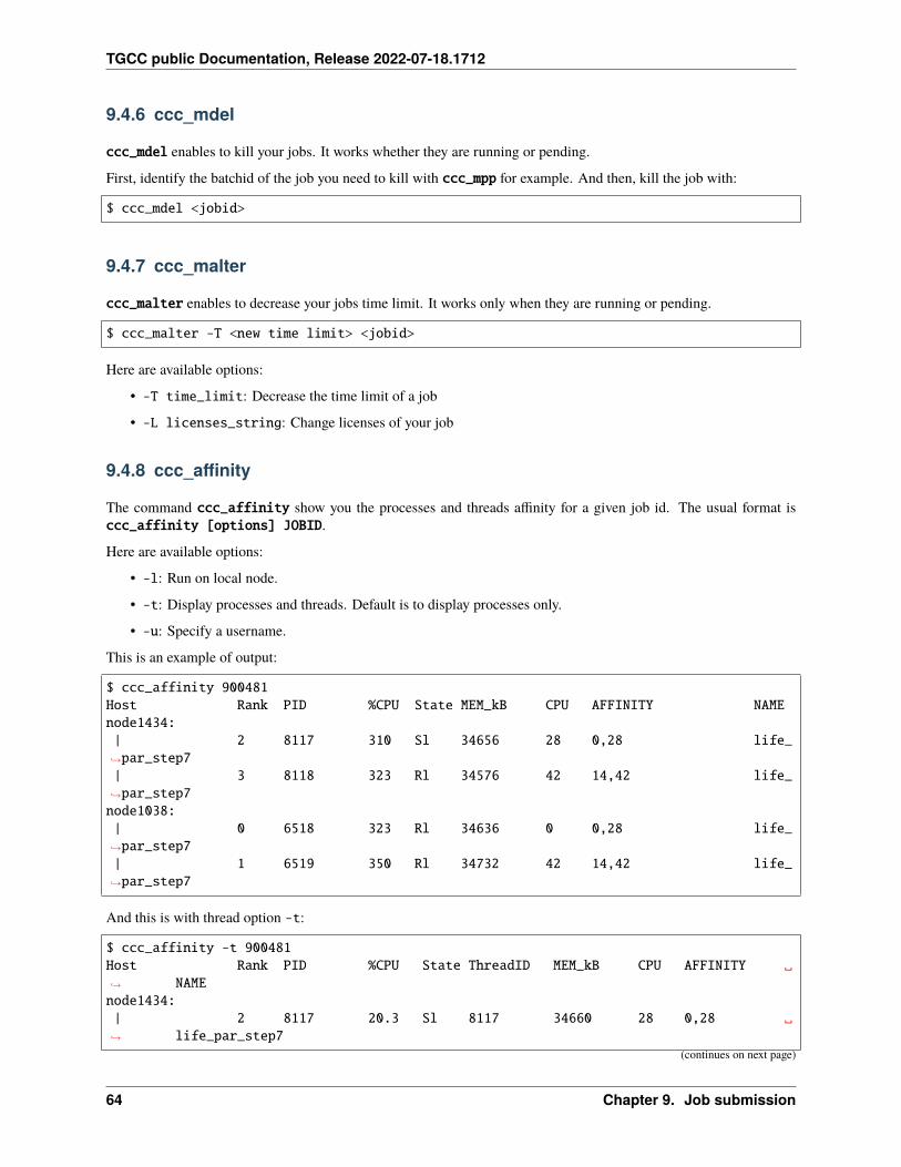
TGCC public Documentation, Release 2022-07-18.1712
9.4.6 ccc_mdel
ccc_mdel enables to kill your jobs. It works whether they are running or pending.
First, identify the batchid of the job you need to kill with ccc_mpp for example. And then, kill the job with:
$ ccc_mdel <jobid>
9.4.7 ccc_malter
ccc_malter enables to decrease your jobs time limit. It works only when they are running or pending.
$ ccc_malter -T <new time limit> <jobid>
Here are available options:
• -T time_limit: Decrease the time limit of a job
• -L licenses_string: Change licenses of your job
9.4.8 ccc_affinity
The command ccc_affinity show you the processes and threads affinity for a given job id. The usual format isccc_affinity [options] JOBID.
Here are available options:
• -l: Run on local node.
• -t: Display processes and threads. Default is to display processes only.
• -u: Specify a username.
This is an example of output:
$ ccc_affinity 900481Host Rank PID %CPU State MEM_kB CPU AFFINITY NAMEnode1434:| 2 8117 310 Sl 34656 28 0,28 life_→˓par_step7| 3 8118 323 Rl 34576 42 14,42 life_→˓par_step7node1038:| 0 6518 323 Rl 34636 0 0,28 life_→˓par_step7| 1 6519 350 Rl 34732 42 14,42 life_→˓par_step7
And this is with thread option -t:
$ ccc_affinity -t 900481Host Rank PID %CPU State ThreadID MEM_kB CPU AFFINITY ␣→˓ NAMEnode1434:| 2 8117 20.3 Sl 8117 34660 28 0,28 ␣→˓ life_par_step7
(continues on next page)
64 Chapter 9. Job submission
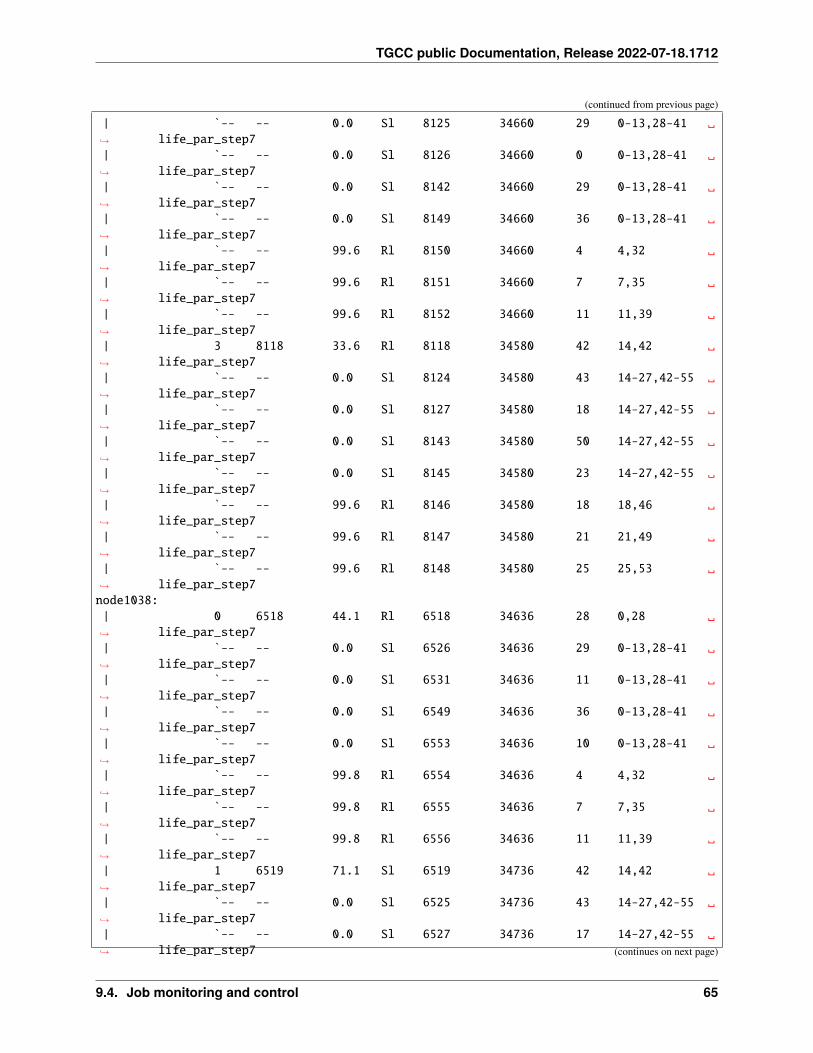
TGCC public Documentation, Release 2022-07-18.1712
(continued from previous page)
| `-- -- 0.0 Sl 8125 34660 29 0-13,28-41 ␣→˓ life_par_step7| `-- -- 0.0 Sl 8126 34660 0 0-13,28-41 ␣→˓ life_par_step7| `-- -- 0.0 Sl 8142 34660 29 0-13,28-41 ␣→˓ life_par_step7| `-- -- 0.0 Sl 8149 34660 36 0-13,28-41 ␣→˓ life_par_step7| `-- -- 99.6 Rl 8150 34660 4 4,32 ␣→˓ life_par_step7| `-- -- 99.6 Rl 8151 34660 7 7,35 ␣→˓ life_par_step7| `-- -- 99.6 Rl 8152 34660 11 11,39 ␣→˓ life_par_step7| 3 8118 33.6 Rl 8118 34580 42 14,42 ␣→˓ life_par_step7| `-- -- 0.0 Sl 8124 34580 43 14-27,42-55 ␣→˓ life_par_step7| `-- -- 0.0 Sl 8127 34580 18 14-27,42-55 ␣→˓ life_par_step7| `-- -- 0.0 Sl 8143 34580 50 14-27,42-55 ␣→˓ life_par_step7| `-- -- 0.0 Sl 8145 34580 23 14-27,42-55 ␣→˓ life_par_step7| `-- -- 99.6 Rl 8146 34580 18 18,46 ␣→˓ life_par_step7| `-- -- 99.6 Rl 8147 34580 21 21,49 ␣→˓ life_par_step7| `-- -- 99.6 Rl 8148 34580 25 25,53 ␣→˓ life_par_step7node1038:| 0 6518 44.1 Rl 6518 34636 28 0,28 ␣→˓ life_par_step7| `-- -- 0.0 Sl 6526 34636 29 0-13,28-41 ␣→˓ life_par_step7| `-- -- 0.0 Sl 6531 34636 11 0-13,28-41 ␣→˓ life_par_step7| `-- -- 0.0 Sl 6549 34636 36 0-13,28-41 ␣→˓ life_par_step7| `-- -- 0.0 Sl 6553 34636 10 0-13,28-41 ␣→˓ life_par_step7| `-- -- 99.8 Rl 6554 34636 4 4,32 ␣→˓ life_par_step7| `-- -- 99.8 Rl 6555 34636 7 7,35 ␣→˓ life_par_step7| `-- -- 99.8 Rl 6556 34636 11 11,39 ␣→˓ life_par_step7| 1 6519 71.1 Sl 6519 34736 42 14,42 ␣→˓ life_par_step7| `-- -- 0.0 Sl 6525 34736 43 14-27,42-55 ␣→˓ life_par_step7| `-- -- 0.0 Sl 6527 34736 17 14-27,42-55 ␣→˓ life_par_step7 (continues on next page)
9.4. Job monitoring and control 65
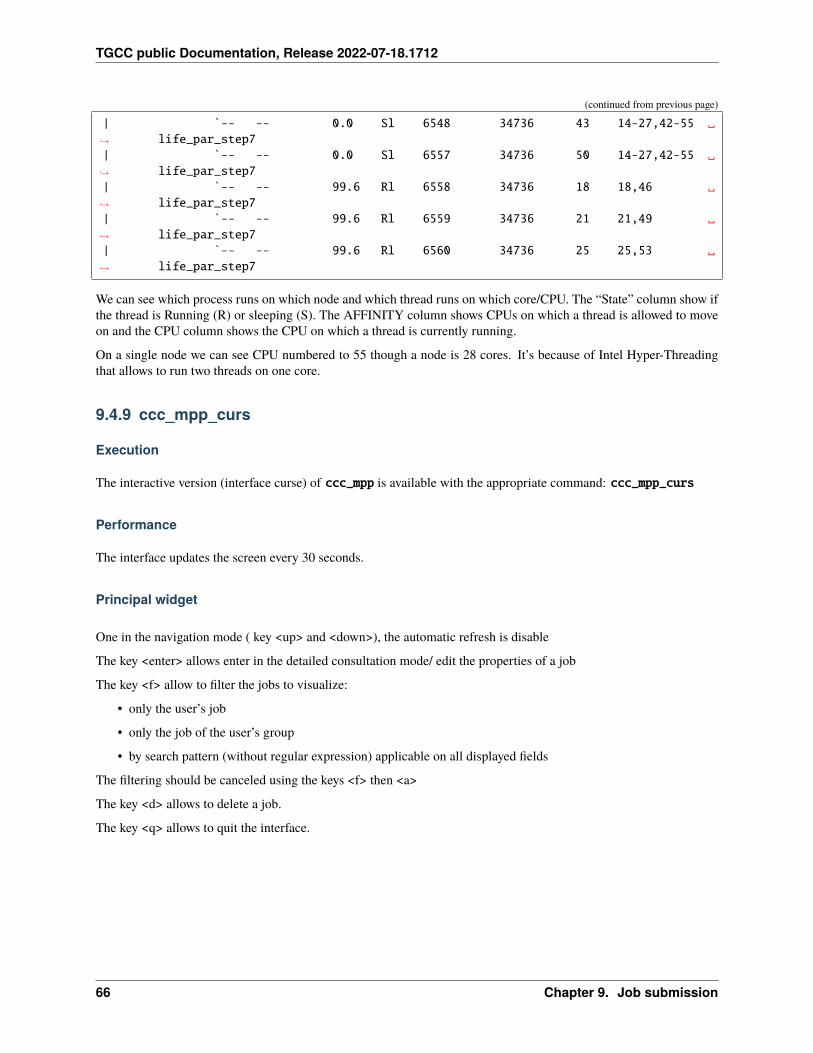
TGCC public Documentation, Release 2022-07-18.1712
(continued from previous page)
| `-- -- 0.0 Sl 6548 34736 43 14-27,42-55 ␣→˓ life_par_step7| `-- -- 0.0 Sl 6557 34736 50 14-27,42-55 ␣→˓ life_par_step7| `-- -- 99.6 Rl 6558 34736 18 18,46 ␣→˓ life_par_step7| `-- -- 99.6 Rl 6559 34736 21 21,49 ␣→˓ life_par_step7| `-- -- 99.6 Rl 6560 34736 25 25,53 ␣→˓ life_par_step7
We can see which process runs on which node and which thread runs on which core/CPU. The “State” column show ifthe thread is Running (R) or sleeping (S). The AFFINITY column shows CPUs on which a thread is allowed to moveon and the CPU column shows the CPU on which a thread is currently running.
On a single node we can see CPU numbered to 55 though a node is 28 cores. It’s because of Intel Hyper-Threadingthat allows to run two threads on one core.
9.4.9 ccc_mpp_curs
Execution
The interactive version (interface curse) of ccc_mpp is available with the appropriate command: ccc_mpp_curs
Performance
The interface updates the screen every 30 seconds.
Principal widget
One in the navigation mode ( key <up> and <down>), the automatic refresh is disable
The key <enter> allows enter in the detailed consultation mode/ edit the properties of a job
The key <f> allow to filter the jobs to visualize:
• only the user’s job
• only the job of the user’s group
• by search pattern (without regular expression) applicable on all displayed fields
The filtering should be canceled using the keys <f> then <a>
The key <d> allows to delete a job.
The key <q> allows to quit the interface.
66 Chapter 9. Job submission
TGCC public Documentation, Release 2022-07-18.1712
Widget of the properties of the job
The navigation is also done with the keys <up> and <down>.
The key <enter> enables to edit a property.
Once all the modifications are done on a job the can be submitted using the key <w>.
The key <q> enables to exit the mode and to cancel the modifications to be submitted.
Edition mode
global constraints
Only the jobs in mode “pending” are editable by their owner.
Achievable actions on jobs
As an owner of a job, one can do the following actions:
• delete a job
• Modification of the following properties
– account: the account on which the job is charged
– fileSystem: change the file system required by the job
– jobname: the name of the job
– LicensesApp: the license required by the job (format Slurm)
– NumCpus: the number of required CPU
– partition: the partition
– QOS: change the Quality of Service
– TimeLimit: the duration of the job
– usage limit: the treashold of the job
Role of the coordinator
The person in charge of imputation may request to be referenced as coordinator to the TGCC hotline.
The user with the role of coordinator has additional rights to interact with all imputation jobs.
9.4. Job monitoring and control 67
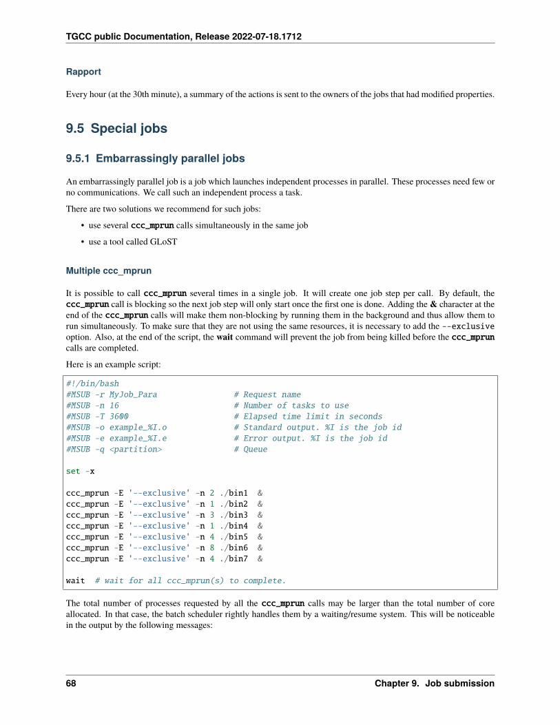
TGCC public Documentation, Release 2022-07-18.1712
Rapport
Every hour (at the 30th minute), a summary of the actions is sent to the owners of the jobs that had modified properties.
9.5 Special jobs
9.5.1 Embarrassingly parallel jobs
An embarrassingly parallel job is a job which launches independent processes in parallel. These processes need few orno communications. We call such an independent process a task.
There are two solutions we recommend for such jobs:
• use several ccc_mprun calls simultaneously in the same job
• use a tool called GLoST
Multiple ccc_mprun
It is possible to call ccc_mprun several times in a single job. It will create one job step per call. By default, theccc_mprun call is blocking so the next job step will only start once the first one is done. Adding the & character at theend of the ccc_mprun calls will make them non-blocking by running them in the background and thus allow them torun simultaneously. To make sure that they are not using the same resources, it is necessary to add the --exclusiveoption. Also, at the end of the script, the wait command will prevent the job from being killed before the ccc_mpruncalls are completed.
Here is an example script:
#!/bin/bash#MSUB -r MyJob_Para # Request name#MSUB -n 16 # Number of tasks to use#MSUB -T 3600 # Elapsed time limit in seconds#MSUB -o example_%I.o # Standard output. %I is the job id#MSUB -e example_%I.e # Error output. %I is the job id#MSUB -q <partition> # Queue
set -x
ccc_mprun -E '--exclusive' -n 2 ./bin1 &ccc_mprun -E '--exclusive' -n 1 ./bin2 &ccc_mprun -E '--exclusive' -n 3 ./bin3 &ccc_mprun -E '--exclusive' -n 1 ./bin4 &ccc_mprun -E '--exclusive' -n 4 ./bin5 &ccc_mprun -E '--exclusive' -n 8 ./bin6 &ccc_mprun -E '--exclusive' -n 4 ./bin7 &
wait # wait for all ccc_mprun(s) to complete.
The total number of processes requested by all the ccc_mprun calls may be larger than the total number of coreallocated. In that case, the batch scheduler rightly handles them by a waiting/resume system. This will be noticeablein the output by the following messages:
68 Chapter 9. Job submission
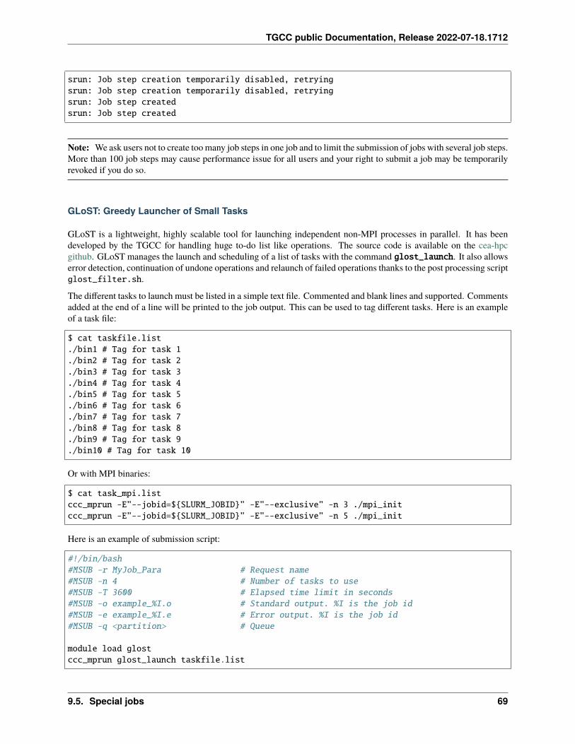
TGCC public Documentation, Release 2022-07-18.1712
srun: Job step creation temporarily disabled, retryingsrun: Job step creation temporarily disabled, retryingsrun: Job step createdsrun: Job step created
Note: We ask users not to create too many job steps in one job and to limit the submission of jobs with several job steps.More than 100 job steps may cause performance issue for all users and your right to submit a job may be temporarilyrevoked if you do so.
GLoST: Greedy Launcher of Small Tasks
GLoST is a lightweight, highly scalable tool for launching independent non-MPI processes in parallel. It has beendeveloped by the TGCC for handling huge to-do list like operations. The source code is available on the cea-hpcgithub. GLoST manages the launch and scheduling of a list of tasks with the command glost_launch. It also allowserror detection, continuation of undone operations and relaunch of failed operations thanks to the post processing scriptglost_filter.sh.
The different tasks to launch must be listed in a simple text file. Commented and blank lines and supported. Commentsadded at the end of a line will be printed to the job output. This can be used to tag different tasks. Here is an exampleof a task file:
$ cat taskfile.list./bin1 # Tag for task 1./bin2 # Tag for task 2./bin3 # Tag for task 3./bin4 # Tag for task 4./bin5 # Tag for task 5./bin6 # Tag for task 6./bin7 # Tag for task 7./bin8 # Tag for task 8./bin9 # Tag for task 9./bin10 # Tag for task 10
Or with MPI binaries:
$ cat task_mpi.listccc_mprun -E"--jobid=${SLURM_JOBID}" -E"--exclusive" -n 3 ./mpi_initccc_mprun -E"--jobid=${SLURM_JOBID}" -E"--exclusive" -n 5 ./mpi_init
Here is an example of submission script:
#!/bin/bash#MSUB -r MyJob_Para # Request name#MSUB -n 4 # Number of tasks to use#MSUB -T 3600 # Elapsed time limit in seconds#MSUB -o example_%I.o # Standard output. %I is the job id#MSUB -e example_%I.e # Error output. %I is the job id#MSUB -q <partition> # Queue
module load glostccc_mprun glost_launch taskfile.list
9.5. Special jobs 69
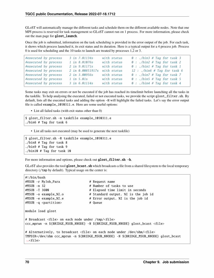
TGCC public Documentation, Release 2022-07-18.1712
GLoST will automatically manage the different tasks and schedule them on the different available nodes. Note that oneMPI process is reserved for task management so GLoST cannot run on 1 process. For more information, please checkout the man page for glost_launch.
Once the job is submitted, information on the task scheduling is provided in the error output of the job. For each task,it shows which process launched it, its exit status and its duration. Here is a typical output for a 4 process job. Process0 is used for scheduling and the 10 tasks to launch are treated by processes 1,2 or 3.
#executed by process 3 in 7.01134s with status 0 : ./bin3 # Tag for task 3#executed by process 1 in 8.01076s with status 0 : ./bin2 # Tag for task 2#executed by process 2 in 9.01171s with status 0 : ./bin1 # Tag for task 1#executed by process 2 in 0.00851917s with status 12 : ./bin6 # Tag for task 6#executed by process 2 in 3.00956s with status 0 : ./bin7 # Tag for task 7#executed by process 1 in 5.01s with status 0 : ./bin5 # Tag for task 5#executed by process 3 in 6.01114s with status 0 : ./bin4 # Tag for task 4
Some tasks may exit on errors or not be executed if the job has reached its timelimit before launching all the tasks inthe taskfile. To help analysing the executed, failed or not executed tasks, we provide the script glost_filter.sh. Bydefault, lists all the executed tasks and adding the option -H will highlight the failed tasks. Let’s say the error outputfile is called example_1050311.e. Here are some useful options:
• List all failed tasks (with exit status other than 0)
$ glost_filter.sh -n taskfile example_1050311.e./bin6 # Tag for task 6
• List all tasks not executed (may be used to generate the next taskfile)
$ glost_filter.sh -R taskfile example_1050311.e./bin8 # Tag for task 8./bin9 # Tag for task 9./bin10 # Tag for task 10
For more information and options, please check out glost_filter.sh -h.
GLoST also provides the tool glost_bcast.shwhich broadcasts a file from a shared filesystem to the local temporarydirectory (/tmp by default). Typical usage on the center is:
#!/bin/bash#MSUB -r MyJob_Para # Request name#MSUB -n 32 # Number of tasks to use#MSUB -T 3600 # Elapsed time limit in seconds#MSUB -o example_%I.o # Standard output. %I is the job id#MSUB -e example_%I.e # Error output. %I is the job id#MSUB -q <partition> # Queue
module load glost
# Broadcast <file> on each node under /tmp/<file>ccc_mprun -n ${BRIDGE_MSUB_NNODE} -N ${BRIDGE_MSUB_NNODE} glost_bcast <file>
# Alternatively, to broadcast <file> on each node under /dev/shm/<file>TMPDIR=/dev/shm ccc_mprun -n ${BRIDGE_MSUB_NNODE} -N ${BRIDGE_MSUB_NNODE} glost_bcast→˓<file>
70 Chapter 9. Job submission
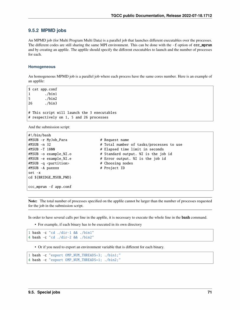
TGCC public Documentation, Release 2022-07-18.1712
9.5.2 MPMD jobs
An MPMD job (for Multi Program Multi Data) is a parallel job that launches different executables over the processes.The different codes are still sharing the same MPI environment. This can be done with the -f option of ccc_mprunand by creating an appfile. The appfile should specify the different executables to launch and the number of processesfor each.
Homogeneous
An homogeneous MPMD job is a parallel job where each process have the same cores number. Here is an example ofan appfile:
$ cat app.conf1 ./bin15 ./bin226 ./bin3
# This script will launch the 3 executables# respectively on 1, 5 and 26 processes
And the submission script:
#!/bin/bash#MSUB -r MyJob_Para # Request name#MSUB -n 32 # Total number of tasks/processes to use#MSUB -T 1800 # Elapsed time limit in seconds#MSUB -o example_%I.o # Standard output. %I is the job id#MSUB -e example_%I.e # Error output. %I is the job id#MSUB -q <partition> # Choosing nodes#MSUB -A paxxxx # Project IDset -xcd ${BRIDGE_MSUB_PWD}
ccc_mprun -f app.conf
Note: The total number of processes specified on the appfile cannot be larger than the number of processes requestedfor the job in the submission script.
In order to have several calls per line in the appfile, it is necessary to execute the whole line in the bash command.
• For example, if each binary has to be executed in its own directory
1 bash -c "cd ./dir-1 && ./bin1"4 bash -c "cd ./dir-2 && ./bin2"
• Or if you need to export an environment variable that is different for each binary.
1 bash -c "export OMP_NUM_THREADS=3; ./bin1;"4 bash -c "export OMP_NUM_THREADS=1; ./bin2;"
9.5. Special jobs 71
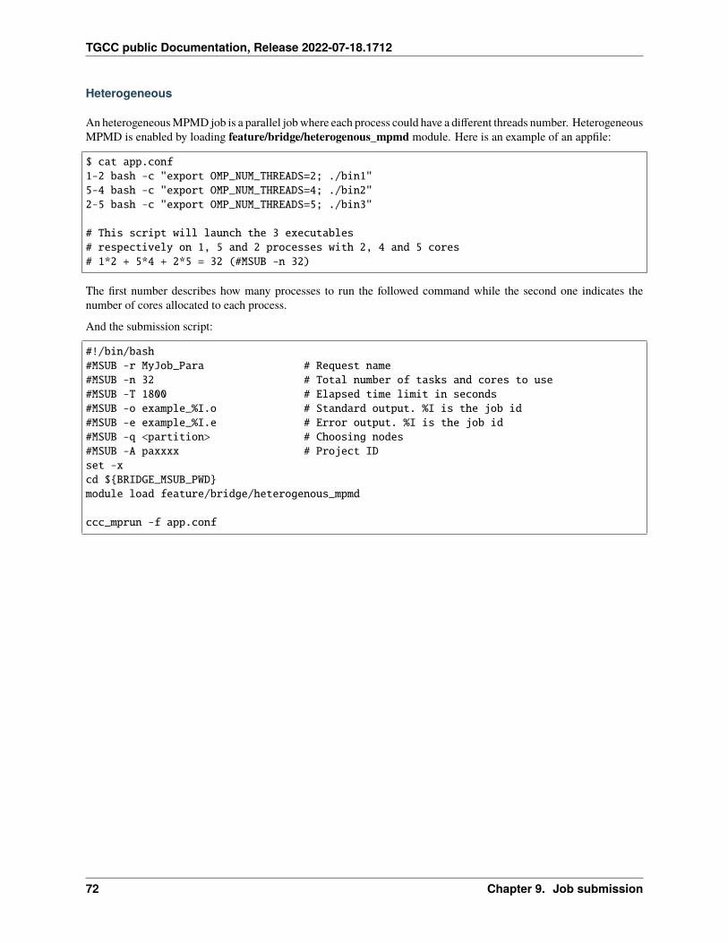
TGCC public Documentation, Release 2022-07-18.1712
Heterogeneous
An heterogeneous MPMD job is a parallel job where each process could have a different threads number. HeterogeneousMPMD is enabled by loading feature/bridge/heterogenous_mpmd module. Here is an example of an appfile:
$ cat app.conf1-2 bash -c "export OMP_NUM_THREADS=2; ./bin1"5-4 bash -c "export OMP_NUM_THREADS=4; ./bin2"2-5 bash -c "export OMP_NUM_THREADS=5; ./bin3"
# This script will launch the 3 executables# respectively on 1, 5 and 2 processes with 2, 4 and 5 cores# 1*2 + 5*4 + 2*5 = 32 (#MSUB -n 32)
The first number describes how many processes to run the followed command while the second one indicates thenumber of cores allocated to each process.
And the submission script:
#!/bin/bash#MSUB -r MyJob_Para # Request name#MSUB -n 32 # Total number of tasks and cores to use#MSUB -T 1800 # Elapsed time limit in seconds#MSUB -o example_%I.o # Standard output. %I is the job id#MSUB -e example_%I.e # Error output. %I is the job id#MSUB -q <partition> # Choosing nodes#MSUB -A paxxxx # Project IDset -xcd ${BRIDGE_MSUB_PWD}module load feature/bridge/heterogenous_mpmd
ccc_mprun -f app.conf
72 Chapter 9. Job submission
CHAPTER
TEN
PROJECT ACCOUNTING
10.1 Computing hours consumption control process
To guarantee a smooth and fair use of the computing resources available on Irene, projects must use their awarded corehours on a regular basis without being late.
To encourage users to respect this rule, projects consumption is automatically and periodically checked. In case ofunder-consumption, the number of core hours awarded gets reduced. On the other hand, this mechanism doesn’t preventover-consumption.
The process respects the following rules:
• The 15th of each month, the current accounting of each project is compared with the theoretical one (awardedhours / total number of days in project * elapsed number of days).
• Between 30 days and 59 days of lateness, an e-mail warns the project leader.
• If a project has more than 60 days of lateness, a 30-days amount of core hours is deducted from the global awardedcore hours.
Note:
• This process concerns PRACE Regular Access projects and over-a-million-hour GENCI projects.
• At any time, users can check their project accounting with the “ccc_myproject” command.
• No hour will be subtracted without a warning e-mail being sent a month beforehand.
• Derogation requests must be sent to the TGCC Hotline.
In case of over-consumption, jobs still can be run. They will run only if there is no job from a nominal-consuming orfrom an under-consuming project in queue waiting for computing resources. A running job from an over-consumingproject is called a “bonus job”. This mechanism is automatically managed by the scheduler and no option is necessaryto use it. For DARI projects, the project is closed when the consumed hours reach 125% of the granted hours amountand can therefore consume more than the initially granted hours amount if it has benefited of bonus jobs.
73
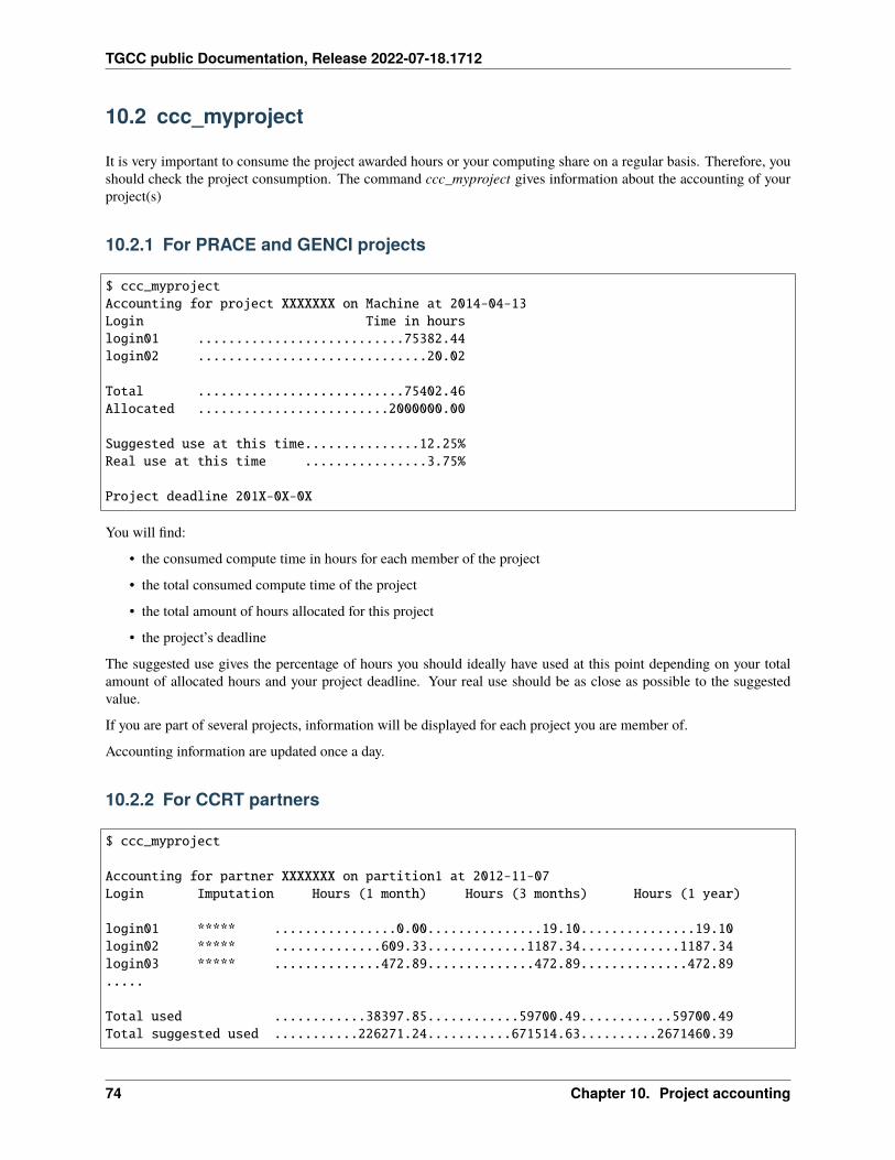
TGCC public Documentation, Release 2022-07-18.1712
10.2 ccc_myproject
It is very important to consume the project awarded hours or your computing share on a regular basis. Therefore, youshould check the project consumption. The command ccc_myproject gives information about the accounting of yourproject(s)
10.2.1 For PRACE and GENCI projects
$ ccc_myprojectAccounting for project XXXXXXX on Machine at 2014-04-13Login Time in hourslogin01 ...........................75382.44login02 ..............................20.02
Total ...........................75402.46Allocated .........................2000000.00
Suggested use at this time...............12.25%Real use at this time ................3.75%
Project deadline 201X-0X-0X
You will find:
• the consumed compute time in hours for each member of the project
• the total consumed compute time of the project
• the total amount of hours allocated for this project
• the project’s deadline
The suggested use gives the percentage of hours you should ideally have used at this point depending on your totalamount of allocated hours and your project deadline. Your real use should be as close as possible to the suggestedvalue.
If you are part of several projects, information will be displayed for each project you are member of.
Accounting information are updated once a day.
10.2.2 For CCRT partners
$ ccc_myproject
Accounting for partner XXXXXXX on partition1 at 2012-11-07Login Imputation Hours (1 month) Hours (3 months) Hours (1 year)
login01 ***** ................0.00...............19.10...............19.10login02 ***** ..............609.33.............1187.34.............1187.34login03 ***** ..............472.89..............472.89..............472.89.....
Total used ............38397.85............59700.49............59700.49Total suggested used ...........226271.24...........671514.63..........2671460.39
74 Chapter 10. Project accounting
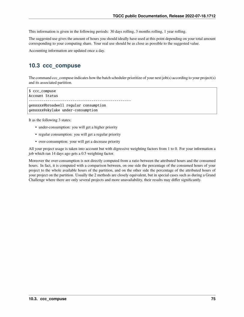
TGCC public Documentation, Release 2022-07-18.1712
This information is given in the following periods: 30 days rolling, 3 months rolling, 1 year rolling.
The suggested use gives the amount of hours you should ideally have used at this point depending on your total amountcorresponding to your computing share. Your real use should be as close as possible to the suggested value.
Accounting information are updated once a day.
10.3 ccc_compuse
The command ccc_compuse indicates how the batch scheduler prioritize of your next job(s) according to your project(s)and its associated partition.
$ ccc_compuseAccount Status-------------------------------------------------genxxxx@broadwell regular consumptiongenxxxx@skylake under-consumption
It as the following 3 states:
• under-consumption: you will get a higher priority
• regular consumption: you will get a regular priority
• over-consumption: your will get a decrease priority
All your project usage is taken into account but with digressive weighting factors from 1 to 0. For your information ajob which ran 14 days ago gets a 0.5 weighting factor.
Moreover the over-consumption is not directly computed from a ratio between the attributed hours and the consumedhours. In fact, it is computed with a comparison between, on one side the percentage of the consumed hours of yourproject to the whole available hours of the partition, and on the other side the percentage of the attributed hours ofyour project on the partition. Usually the 2 methods are closely equivalent, but in special cases such as during a GrandChallenge where there are only several projects and more unavailability, their results may differ significantly.
10.3. ccc_compuse 75

TGCC public Documentation, Release 2022-07-18.1712
76 Chapter 10. Project accounting
CHAPTER
ELEVEN
COMPILATION
11.1 Language standard
The most of IT languages are ruled by some entities called norme or standard. Those entities define explicitly thepurpose of a language, how to use it, and how users should use it. For example the C language have several standards:
• K&R C
• ANSI C (C89) – ISO C (C90)
• C99
• C11
• C embedded
Each standard comes with changes and new features, and most of it are just a revision of the current standard. Nowadaysthe Intel Suite compilers covers the last release of the different standards existing for the C, C++ and Fortran languages.Since the covers of a standard is compiler dependent, users should be aware of the different features implemented bylooking at the official website.
11.2 Available compilers
Several well-known compilers are available for the C, C++ and Fortran languages. The most common being:
• Intel Compiler suite (icc, icpc, ifort)
• GNU compiler suite (gcc, g++, gfortran)
To get a complete list of available compilers and versions use the search parameter of module
$ module search compiler
We recommend to use the Intel Compiler Suite for better performances.
Here is how you would basically compile a serial code
$ icc [options] -o serial_prog.exe serial_prog.c$ icpc [options] -o serial_prog.exe serial_prog.cpp$ ifort [options] -o serial_prog.exe serial_prog.f90
77
TGCC public Documentation, Release 2022-07-18.1712
11.2.1 Intel
Compiler flags
The following sections are an overview of the most frequent options for each compiler.
C/C++
The Intel compilers icc and icpc use mostly the same options. Their behaviors differ slightly: icpc assumes that allsource files are C++, whereas icc distinguishes between .c and .cpp filenames.
Basic flags:
• -o exe_file: names the executable exe_file
• -c: generates the corresponding object file, without creating an executable.
• -g: compiles with the debug symbols.
• -I dir_name: specifies the path of the include files.
• -L dir_name: specifies the path of the libraries.
• -l bib: asks to link the libbib.a library
Preprocessor:
• -E: preprocess the files and sends the result to the standard output
• -P: preprocess the files and sends the result in file.i
• -Dname=: defines the name variable
• -M: creates a list of dependencies
Practical:
• -p: profiling with gprof (needed at compilation time)
• -mp, -mp1: IEEE arithmetic, mp1 is a compromise between time and accuracy
To tell the compiler to conform to a specific language standard :
• -std=val: where val can take the following values (cf. man icc or man icpc)
– c++14 : Enables support for the 2014 ISO C++ standard features.
– c++11 : Enables support for many C++11 (formerly known as C++0x) features.
– C99 : Conforms to The ISO/IEC 9899:1999 International Standard for the C language.
– . . .
Note: If the desired standard is not fully supported by the current version of the Intel compiler (some features of thestandard are not yet implemented), it might be supported by the last version of the GNU compilers. Since the Intelsuit compilers are compiled against the gcc system (the one from the OS), load a recent version of the GNU compilersmight solve this issue.
78 Chapter 11. Compilation
TGCC public Documentation, Release 2022-07-18.1712
Fortran
The Intel compiler for Fortran is ifort.
Basic flags:
• -o exe_file: name the executable exe_file
• -c: generate the object file without creating an executable.
• -g: compile with the debug symbols.
• -I dir_name: add dir_name to the list of directories where include files are looked for.
• -L dir_name: add dir_name to the list of directories where libraries are looked for.
• -l bib: link the libbib.a library
Run-time check
• -C or -check: generates a code which ends up in ‘run time error’ (ex: segmentation fault)
Preprocessor:
• -E: pre-process the files and send the result to the standard output
• -P: pre-process the files and send the result to file.i
• -Dname=: assign the value value to the variable name
• -M: creates a list of dependencies
• -fpp: pre-process the files and compile
Practical:
• -p: compile for profiling with gprof. You will not be able to use gprof otherwise.
• -mp, -mp1: IEEE arithmetic (mp1 is a compromise between time and accuracy)
• -i8: promote integers to 64 bits by default
• -r8: promote reals to 64 bits by default
• -module dir: send/read the files *.mod in the dir directory
• -fp-model strict: strictly adhere to value-safe optimizations when implementing floating-point calculations,and enable floating-point exception semantics. This may slow down your program.
To tell the compiler to conform to a specific language standard :
• -stand=val: where val can take the following values (cf. man ifort)
– f15: Issues messages for language elements that are not standard in draft Fortran 2015.
– f08: Tells the compiler to issue messages for language elements that are not standard in Fortran 2008
– f03: Tells the compiler to issue messages for language elements that are not standard in Fortran 2003
– . . .
Note: Please refer to the man pages for more information about the compilers.
11.2. Available compilers 79
TGCC public Documentation, Release 2022-07-18.1712
Optimization flags
Compilers provide many optimization options: this section describes them.
Basic optimization options :
• -O0, -O1, -O2, -O3: optimization levels - default: -O2
• -opt_report : writes an optimization report to stderr (-O3 required)
• -ip, -ipo: inter-procedural optimizations (mono and multi files). The command xiar must be used instead of arto generate a static library file with objects compiled with -ipo option.
• -fast : default high optimization level (-O3 -ipo -static).
• -ftz : considers all the denormalized numbers (like INF or NAN) as zeros at runtime.
• -fp-relaxed : mathematical optimization functions. Leads to a small loss of accuracy.
• -pad : makes the modification of the memory positions operational (ifort only)
Warning: The -fast option is not allowed with MPI because the MPI context needs some libraries which onlyexist in dynamic mode. This is incompatible with the -static option. You need to replace -fast by -O3 -ipo.
Vectorization flags
Some options allow to use specific vectorization instructions of Intel processors to optimize the code. They are com-patible with most Intel processors. The compiler will try to generate these instructions if the processor allows them.
• -xcode : Tells the compiler which processor features it may target, including which instruction sets and opti-mization it may generate. “code” is one of the following:
– CORE-AVX2
– AVX
– SSE4.2
– SSE2
• -xHost : Applies the highest level of vectorization supported depending on the processor where the compilationis performed. The login nodes may not have the same level of support as the compute nodes. So this option is tobe used only if the compilation is done on the targeted compute nodes.
• -axcode : Tells the compiler to generate a single executable with multiple levels of vectorization. “code” is acomma-separated list of instructions sets.
The default level of vectorization is sse2. However, it is only be activated for optimization level -O2 and more.
• -vec-report[=n] : depending on the value of n, the option -vec-report enables information reports by thevectorizer.
Warning: A code compiled for a given instruction set will not run on a processor that only supports a lowerinstruction set
80 Chapter 11. Compilation
TGCC public Documentation, Release 2022-07-18.1712
Default compilation flags
By default each of the Intel compiler provide the -sox option which allows to save all the options provided at thecompilation time in the comment section of the ELF binary file. To display the comment section :
$ icc -g -O3 hello.c -o helloworld$ readelf -p .comment ./helloworldString dump of section '.comment':[ 0] GCC: (GNU) <x.y.z> (Red Hat <x.y.z>)[ 2c] -?comment:Intel(R) C Intel(R) 64 Compiler for applications running on␣→˓Intel(R) 64, Version <x.y.z> Build <XXXXXX> : hello.c : -sox -g -O3 -o helloworld
11.2.2 GNU
Compiler flags
Basic flags:
• -o exe_file: names the executable exe_file
• -c: generates the corresponding object file, without creating an executable.
• -g: compiles with the debug symbols.
• -I dir_name: specifies the path where the include files are located.
• -L dir_name: specifies the path where the libraries are located.
• -l bib: asks to link the libbib.a library
To tell the compiler to conform to a specific language standard (g++/gcc/gfortran) :
• -std=val: where val can take the following values (cf. man gcc/g++/gfortran)
– c++14 : Enables support for the 2014 ISO C++ standard features.
– C99 : Conforms to The ISO/IEC 9899:1999 International Standard.
– f03: Tells the compiler to issue messages for language elements that are not standard in Fortran 2003
– f08: Tells the compiler to issue messages for language elements that are not standard in Fortran 2008
– . . .
Below are some specific flags for the gfortran commands.
Debugging:
• -Wall: short for “warn about all”, warns about usual causes of bugs, such as having a subroutine or functionnamed like a built-in one, or passing the same variable as an intent(in) and an intent(out) argument of the samesubroutine
• -Wextra: used with -Wall, warns about even more potential problems, like unused subroutine arguments
• -w: inhibits all warning messages (not recommended)
• -Werror: considers any warning as an error
11.2. Available compilers 81
TGCC public Documentation, Release 2022-07-18.1712
Optimization flags
Compilers provide many optimization options: this section describes them.
Basic optimization options :
• -O0, -O1, -O2, -O3: optimization levels - default: -O0
Some options allow usage of specific set of instructions for Intel processors, to optimize code behavior. They arecompatible with most Intel processors. The compiler will try to use them if the processor allows them.
• -mavx2 / -mno-avx2 : Switch on or off the usage of said instruction set.
• -mavx / -mno-avx : idem.
• -msse4.2 / -mno-sse4.2 : idem.
11.3 Available numerical libraries
11.3.1 MKL library
The Intel MKL library is integrated in the Intel package and contains:
• BLAS, SparseBLAS;
• LAPACK, ScaLAPACK;
• Sparse Solver, CBLAS ;
• Discrete Fourier and Fast Fourier transform
If you don’t need ScaLAPACK:
$ module load mkl$ ifort -o myexe myobject.o ${MKL_LDFLAGS}
If you need ScaLAPACK:
$ module load scalapack$ mpif90 -o myexe myobject.o ${SCALAPACK_LDFLAGS}
We provide multi-threaded versions for compiling with MKL:
$ module load feature/mkl/multi-threaded$ module load mkl$ ifort -o myexe myobject.o ${$MKL_LDFLAGS}
$ module load feature/mkl/multi-threaded$ module load scalapack$ mpif90 -o myexe myobject.o ${SCALAPACK_LDFLAGS}
To use multi-threaded MKL, you have to set the OpenMP environment variable OMP_NUM_THREADS.
We strongly recommend you to use the MKL_XXX and SCALAPACK_XXX environment variables made available by themkl and scalapack modules.
82 Chapter 11. Compilation
TGCC public Documentation, Release 2022-07-18.1712
11.3.2 FFTW
FFTW is a C subroutine library for computing the discrete Fourier transform (DFT) in one or more dimensions, withan arbitrary input size, and with both real and complex data. It is provided by the fftw3/gnu module. The variablesFFTW3_CFLAGS and FFTW3_LDFLAGS should be used to compile a code using fftw routines.
$ module load fftw3/gnu$ icc ${FFTW3_CFLAGS} -o test example_fftw3.c ${FFTW3_LDFLAGS}$ ifort ${FFTW3_FFLAGS} -o test example_fftw3.f90 ${FFTW3_LDFLAGS}
Intel MKL also provides Fourier transform functions. FFTW3 wrappers are able to link programes so that they can useIntel MKL Fourier transforms instead of the FFTW3 library, without changing the source code. The correct compilingoptions are provided by the fftw3/mkl module.
$ module load fftw3/mkl$ icc ${FFTW3_CFLAGS} -o test example_fftw3.c ${FFTW3_LDFLAGS}$ ifort ${FFTW3_FFLAGS} -o test example_fftw3.f90 ${FFTW3_LDFLAGS}
11.4 Compiling for Skylake
With the -ax option, icc and ifort can generate code for several architectures.
For example, from a Broadwell login nodes, you can generate an executable with both AVX2 (Broadwell) and AVX512(Skylake) instructions set. To do so, you need to add the -axCORE-AVX2,CORE-AVX512 option to icc or ifort.
An executable compiled with -axCORE-AVX2,CORE-AVX512 can be run on both Broadwell and Skylake as the bestinstruction set available on the architecture will be chosen.
11.5 Compiling for Rome/Milan
With the -m option, icc and ifort can generate specific instruction sets for Intel and non-Intel processors.
AMD Rome and Milan processors are able to run AVX2 instructions. To generate an AVX2 instructions for AMDprocessors, you need to add the -mavx2 option to icc or ifort. An executable compiled with -mavx2 can run onboth AMD and Intel processors.
Note:
• The -mavx2 option is compatible with gcc.
• Both -mavx2 and -axCORE-AVX2,CORE-AVX512 options can be used simultaneously with icc and ifort togenerate both specific instructions for Intel processors and more generic instructions for AMD processors.
11.4. Compiling for Skylake 83

TGCC public Documentation, Release 2022-07-18.1712
84 Chapter 11. Compilation
CHAPTER
TWELVE
PARALLEL PROGRAMMING
12.1 MPI
The MPI (Message Passing Interface) standard is an API for processes that need to send, wait or receive messages. Afull documentation of all the implemented functions can be found in the MPI Standard documentation.
12.1.1 MPI implementations
The supercomputer comes with a default MPI implementation provided by the manufacturer. The supported MPIimplementation is OpenMPI.
Other existing implementations include IntelMPI, MVAPICH2, PlatformMPI but all are not made available on thecluster. To see a list of implementations available, use the command module avail mpi.
The default MPI implementation is loaded in your environment at connexion time.
12.1.2 Compiling MPI programs
You can compile and link MPI programs using the wrappers mpicc, mpic++, mpif77 and mpif90. Those wrappersactually call basic compilers but add the correct paths to MPI include files and linking options to MPI libraries.
For example to compile a simple program using MPI:
$ mpicc -o mpi_prog.exe mpi_prog.c$ mpic++ -o mpi_prog.exe mpi_prog.cpp$ mpif90 -o mpi_prog.exe mpi_prog.f90
To see the full compiling call made by the wrapper, use the command mpicc -show.
12.1.3 Wi4MPI
Interoperability between MPI implementations is usually not possible because each one has a specific ApplicationBinary Interface (ABI). To overcome this, we have Wi4MPI. Wi4MPI provides two modes (Interface and Preload)with the same promise, one compilation for several run on different MPI implementations (OpenMPI, IntelMPI).
85
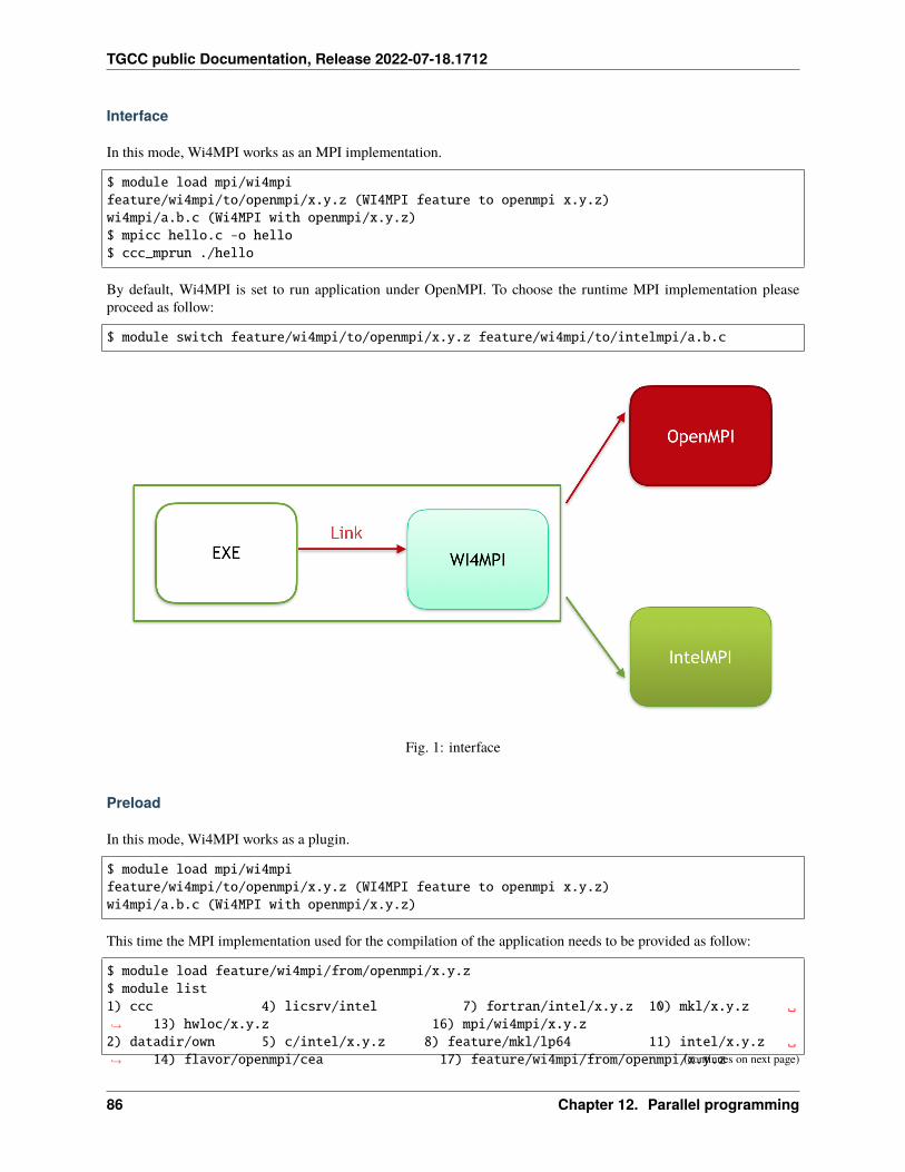
TGCC public Documentation, Release 2022-07-18.1712
Interface
In this mode, Wi4MPI works as an MPI implementation.
$ module load mpi/wi4mpifeature/wi4mpi/to/openmpi/x.y.z (WI4MPI feature to openmpi x.y.z)wi4mpi/a.b.c (Wi4MPI with openmpi/x.y.z)$ mpicc hello.c -o hello$ ccc_mprun ./hello
By default, Wi4MPI is set to run application under OpenMPI. To choose the runtime MPI implementation pleaseproceed as follow:
$ module switch feature/wi4mpi/to/openmpi/x.y.z feature/wi4mpi/to/intelmpi/a.b.c
Fig. 1: interface
Preload
In this mode, Wi4MPI works as a plugin.
$ module load mpi/wi4mpifeature/wi4mpi/to/openmpi/x.y.z (WI4MPI feature to openmpi x.y.z)wi4mpi/a.b.c (Wi4MPI with openmpi/x.y.z)
This time the MPI implementation used for the compilation of the application needs to be provided as follow:
$ module load feature/wi4mpi/from/openmpi/x.y.z$ module list1) ccc 4) licsrv/intel 7) fortran/intel/x.y.z 10) mkl/x.y.z ␣→˓ 13) hwloc/x.y.z 16) mpi/wi4mpi/x.y.z2) datadir/own 5) c/intel/x.y.z 8) feature/mkl/lp64 11) intel/x.y.z ␣→˓ 14) flavor/openmpi/cea 17) feature/wi4mpi/from/openmpi/x.y.z(continues on next page)
86 Chapter 12. Parallel programming
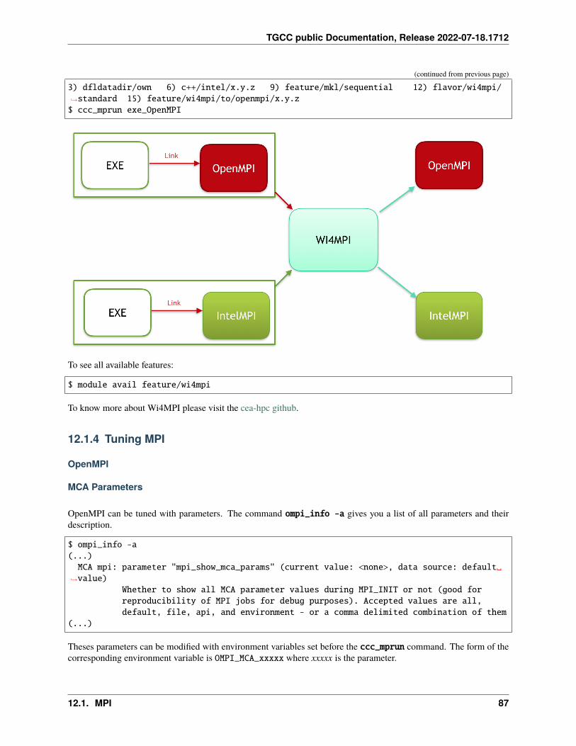
TGCC public Documentation, Release 2022-07-18.1712
(continued from previous page)
3) dfldatadir/own 6) c++/intel/x.y.z 9) feature/mkl/sequential 12) flavor/wi4mpi/→˓standard 15) feature/wi4mpi/to/openmpi/x.y.z$ ccc_mprun exe_OpenMPI
To see all available features:
$ module avail feature/wi4mpi
To know more about Wi4MPI please visit the cea-hpc github.
12.1.4 Tuning MPI
OpenMPI
MCA Parameters
OpenMPI can be tuned with parameters. The command ompi_info -a gives you a list of all parameters and theirdescription.
$ ompi_info -a(...)MCA mpi: parameter "mpi_show_mca_params" (current value: <none>, data source: default␣
→˓value)Whether to show all MCA parameter values during MPI_INIT or not (good forreproducibility of MPI jobs for debug purposes). Accepted values are all,default, file, api, and environment - or a comma delimited combination of them
(...)
Theses parameters can be modified with environment variables set before the ccc_mprun command. The form of thecorresponding environment variable is OMPI_MCA_xxxxx where xxxxx is the parameter.
12.1. MPI 87
TGCC public Documentation, Release 2022-07-18.1712
#!/bin/bash#MSUB -r MyJob_Para # Request name#MSUB -n 32 # Number of tasks to use#MSUB -T 1800 # Elapsed time limit in seconds#MSUB -o example_%I.o # Standard output. %I is the job id#MSUB -e example_%I.e # Error output. %I is the job id#MSUB -A paxxxx # Project ID#MSUB -q partition # Queue
set -xcd ${BRIDGE_MSUB_PWD}export OMPI_MCA_mpi_show_mca_params=allccc_mprun ./a.out
For more information on MCA parameters, check out the tuning part of the openmpi FAQ.
Predefined MPI profiles
Some common MCA parameters are defined in several features (openmpi) to simplify their usage.
Here are those modules:
$ module avail feature/openmpi----------------- /opt/Modules/default/modulefiles/applications ---------------------------------- /opt/Modules/default/modulefiles/environment -----------------feature/openmpi/big_collective_io feature/openmpi/gnu feature/openmpi/mxm feature/→˓openmpi/performance feature/openmpi/performance_test
Here is their description and their limitation(s):
• performance
Description : Improve communication performances in classic applications (namely those with fixedcommunication scheme). Limitation : Moderately increase the memory consumption of the MPIlayer.
• big_collective_io
Description : Increase data bandwidth when accessing big files on lustre file system. Limitation :Only useful when manipulating big files through MPI_IO and derivated (parallel hdf5, etc.).
• collective_performance
Description : Improve the performance of several MPI collective routines by using the GHC featuredeveloped by BULL. Limitation : Improvements may not be seen on small cases. Namely change theorder in which MPI reduction operations are performed and may impact the reproductability and/orthe numerical stability of very sensible systems.
• low_memory_footprint
Description : Reduce the memory consumption of the MPI layer. Limitation : May have strong impactover communication performances. Should only be used when you are near the memory limits.
88 Chapter 12. Parallel programming
TGCC public Documentation, Release 2022-07-18.1712
Compiler Features
By default, MPI wrappers use Intel compilers. To use GNU compilers, you need to set the following environmentvariables:
• OMPI_CC for C
• OMPI_CXX for C++
• OMPI_F77 for fortran77
• OMPI_FC for fortran90
For example:
$ export OMPI_CC=gcc$ mpicc -o test.exe test.c
It’s also possible to use the feature feature/openmpi/gnu which set all variables define above at GNU compilers (gcc,g++, gfortran).
$ module load feature/openmpi/gnuload module feature/openmpi/gnu (OpenMPI profile feature)
IntelMPI
Compiler Features
By default, MPI wrappers use Intel compilers. To use GNU compilers, you need to set the following environmentvariables:
• I_MPI_CC for C
• I_MPI_CXX for C++
• I_MPI_F77 for fortran77
• I_MPI_FC for fortran90
For example:
$ export I_MPI_CC=gcc$ mpicc -o test.exe test.c
It’s also possible to use the feature feature/intelmpi/gnu which set all variables define above at GNU compilers (gcc,g++, gfortran).
$ module load feature/intelmpi/gnuload module feature/intelmpi/gnu (IntelMPI profile feature)
12.1. MPI 89
TGCC public Documentation, Release 2022-07-18.1712
12.2 OpenMP
OpenMP is an API that supports multi-platform shared memory multiprocessing programming in C, C++, and Fortran.It consists of a set of compiler directives, library routines, and environment variables that influence run-time behavior.More information and a full documentation can be found on the official website.
12.2.1 Compiling OpenMP programs
The Intel and GNU compilers both support OpenMP. Use the -fopenmp flag to generate multi-threaded code withthose compilers.
Note: -openmp works only for intel whereas -fopenmp works with both Intel and GNU compilers.
$ icc -fopenmp -o openmp_prog.exe openmp_prog.c$ icpc -fopenmp -o openmp_prog.exe openmp_prog.cpp$ ifort -fopenmp -o openmp_prog.exe openmp_prog.f90
12.2.2 Intel thread affinity
By default, threads inherit the same affinity than their parent process (see Process distribution, affinity and binding formore information). For example, if the parent process has been allocated 4 cores, the OpenMP threads spawned by thisprocess will be allowed to run freely on those 4 cores.
To set a more specific binding for threads among the allocated cores, Intel provides environment variables:KMP_AFFINITY
The values given to KMP_AFFINITY should be a comma-separated list of the following keywords:
• verbose: prints messages concerning the supported affinity.
• granularity=: specifies whether to pin OpenMP threads to physical cores (granularity=core, this is thedefault) or pin to logical cores (granularity=fine). This is only effective on nodes that support hyperthread-ing.
• compact: assigns the threads as close as possible together.
• scatter: distributes the threads as evenly as possible across the entire system.
12.3 Using GPUs
12.3.1 CUDA
The CUDA compiler is available for hybrid nodes to compile GPU-accelerated programs for Nvidia devices.
To compile a simple CUDA code:
$ module load cuda$ nvcc -o test_cuda test.cu
90 Chapter 12. Parallel programming
TGCC public Documentation, Release 2022-07-18.1712
Each new generation of GPU comes with new CUDA features. To use those features in a code, you may need tospecify the compute capability of the target GPU. Check out the kind of GPU provided on the hybrid partition inSupercomputer architecture and check the related compute capability on the nvidia website. For example, to generatea code for a targeted GPU with a 3.5 compute capability:
$ nvcc -gencode arch=compute_35,code=sm_35 -o test_cuda test.cu
You may specify several levels of support if you need the code to run on different GPU generations.
$ nvcc -gencode arch=compute_35,code=sm_35 -gencode arch=compute_30,code=sm_30 -o test_→˓cuda test.cu
The nvcc command uses C and C++ compilers underneath. Compiling with nvcc -v will show the detail of theunderlying compiling calls. By default, the GNU compilers are used. To change the underlying compiler, use theccbin option:
$ nvcc -v -ccbin=icc -o test_cuda test.cu
Most GPU codes are partially composed of basic sequential codes in separate files. They need to be compiled separately:
$ lscuda_file.cu file.c
$ icc -o file.o -c file.c$ nvcc -ccbin=icc -o cuda_file.o -c cuda_file.cu$ icc -o test_cuda -L${CUDA_LIBDIR} -lcudart file.o cuda_file.o
12.3.2 OpenCL
OpenCL is provided both with the CUDA installation and by a separated Intel installation. Compatibility modules areavailable to simply switch from one version to another: opencl/nvidia and opencl/intel.
$ module load opencl/nvidiaor$ module load opencl/intel
$ icc -I${OPENCL_INCDIR} -o test_ocl opencl.c -lOpenCL
12.3. Using GPUs 91
TGCC public Documentation, Release 2022-07-18.1712
92 Chapter 12. Parallel programming
CHAPTER
THIRTEEN
RUNTIME TUNING
13.1 Memory allocation tuning
13.1.1 Feature TBB malloc
Intel TBB (Threading Building Blocks) presents an API (Application Program Interface) that take full advantage ofmulticore performance. Among this API, there is some allocator that could be found in the GNU C Library as malloc orcalloc but performing in a more efficient way inside TBB. The easiest way for an application to benefit from it (withoutany changes within it) is to provide the following librairies to the environment variable LD_PRELOAD, or to use thefeature available on Irene as follow.
$ module load feature/optimization/tbb_malloc
Now, at each use of the command ccc_mprun, any application will benefit from those allocator.
93

TGCC public Documentation, Release 2022-07-18.1712
94 Chapter 13. Runtime tuning
CHAPTER
FOURTEEN
PROCESS DISTRIBUTION, AFFINITY AND BINDING
14.1 Hardware topology
Hardware topology is the organization of cores, processors, sockets, memory, network cards and accelerators (likegraphic cards) in a node. An image of the topology of a node is shown by lstopo. This function comes with hwloc,and you can access it with the command module load hwloc. For example, a simple graphical representation of acompute node layout can be obtained with:
lstopo --no-caches --no-io --of png
14.2 Definitions
We define here some vocabulary:
• Process distribution : the distribution of MPI processes describes how these processes are spread across thecores, sockets or nodes.
• Process affinity : represents the policy of resources management (cores and memory) for processes.
• Process binding : a Linux process can be bound (or stuck or pinned) to one or many cores. It means a processand its threads can run only on a given selection of cores.
The default behavior for distribution, affinity and binding is managed by the batch scheduler through the ccc_mpruncommand. SLURM (Simple Linux Utility for Resource Management) is the batch scheduler for jobs on the supercom-puter. SLURM manages the distribution, affinity and binding of processes even for sequential jobs. That is why werecommend you to use ccc_mprun even for non-MPI codes.
14.3 Process distribution
We present here the most common MPI process distributions. The cluster naturally has a two dimensional distribution.The first level of distribution manages the process layout across nodes and the second level manages process layoutwithin a node, across sockets.
• Distribution across nodes
– block by node: The block distribution method will distribute tasks such that consecutive tasks share a node.
– cyclic by node: The cyclic distribution method will distribute tasks such that consecutive tasks are dis-tributed over consecutive nodes (in a round-robin fashion).
• Distribution across sockets
95
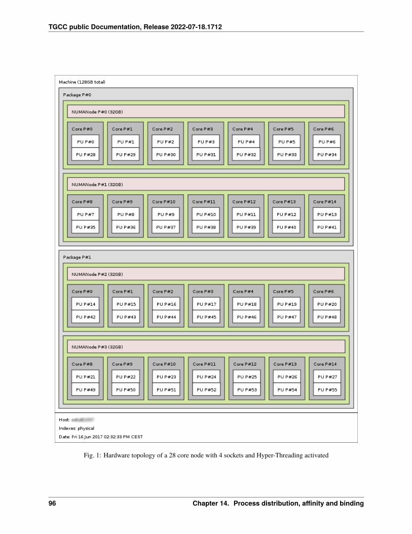
TGCC public Documentation, Release 2022-07-18.1712
Fig. 1: Hardware topology of a 28 core node with 4 sockets and Hyper-Threading activated
96 Chapter 14. Process distribution, affinity and binding
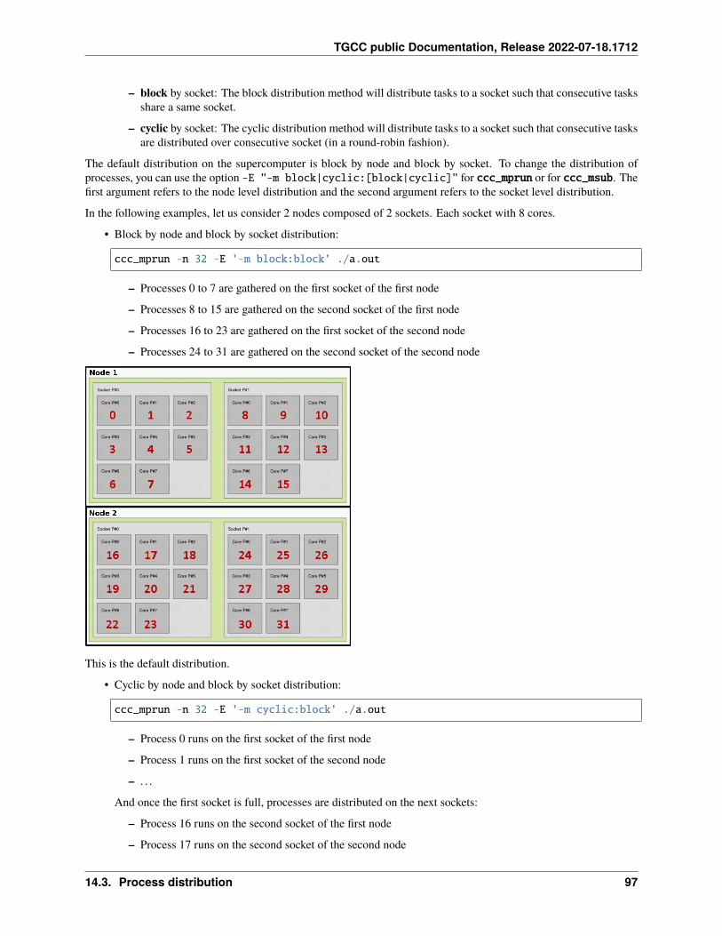
TGCC public Documentation, Release 2022-07-18.1712
– block by socket: The block distribution method will distribute tasks to a socket such that consecutive tasksshare a same socket.
– cyclic by socket: The cyclic distribution method will distribute tasks to a socket such that consecutive tasksare distributed over consecutive socket (in a round-robin fashion).
The default distribution on the supercomputer is block by node and block by socket. To change the distribution ofprocesses, you can use the option -E "-m block|cyclic:[block|cyclic]" for ccc_mprun or for ccc_msub. Thefirst argument refers to the node level distribution and the second argument refers to the socket level distribution.
In the following examples, let us consider 2 nodes composed of 2 sockets. Each socket with 8 cores.
• Block by node and block by socket distribution:
ccc_mprun -n 32 -E '-m block:block' ./a.out
– Processes 0 to 7 are gathered on the first socket of the first node
– Processes 8 to 15 are gathered on the second socket of the first node
– Processes 16 to 23 are gathered on the first socket of the second node
– Processes 24 to 31 are gathered on the second socket of the second node
This is the default distribution.
• Cyclic by node and block by socket distribution:
ccc_mprun -n 32 -E '-m cyclic:block' ./a.out
– Process 0 runs on the first socket of the first node
– Process 1 runs on the first socket of the second node
– . . .
And once the first socket is full, processes are distributed on the next sockets:
– Process 16 runs on the second socket of the first node
– Process 17 runs on the second socket of the second node
14.3. Process distribution 97
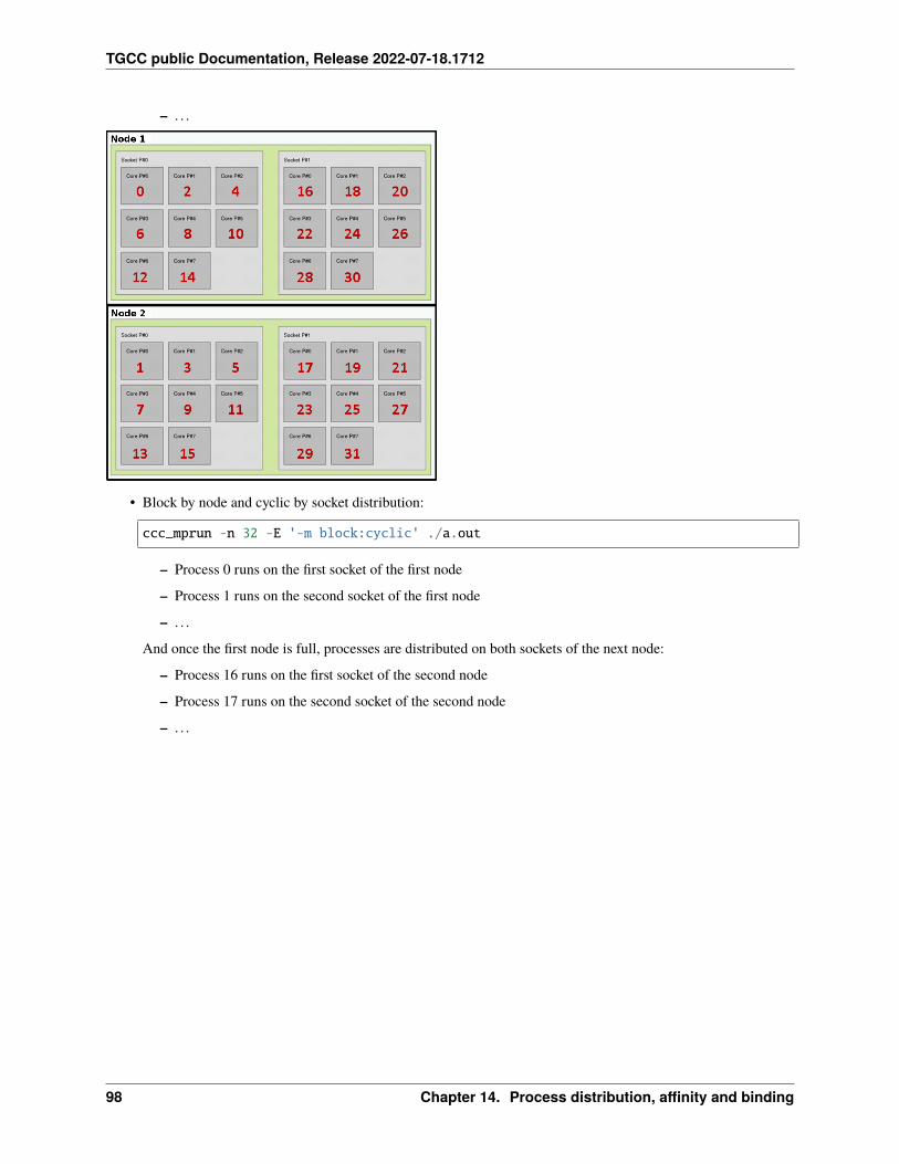
TGCC public Documentation, Release 2022-07-18.1712
– . . .
• Block by node and cyclic by socket distribution:
ccc_mprun -n 32 -E '-m block:cyclic' ./a.out
– Process 0 runs on the first socket of the first node
– Process 1 runs on the second socket of the first node
– . . .
And once the first node is full, processes are distributed on both sockets of the next node:
– Process 16 runs on the first socket of the second node
– Process 17 runs on the second socket of the second node
– . . .
98 Chapter 14. Process distribution, affinity and binding
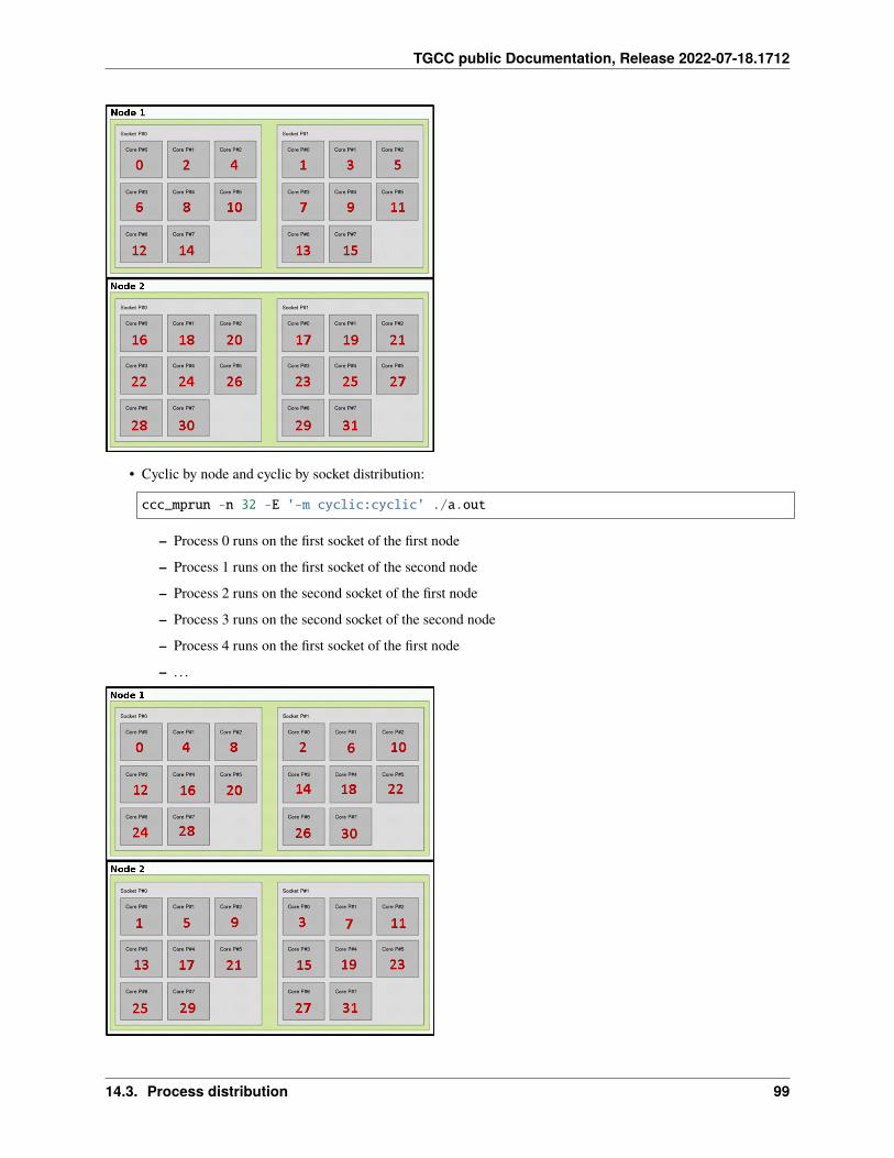
TGCC public Documentation, Release 2022-07-18.1712
• Cyclic by node and cyclic by socket distribution:
ccc_mprun -n 32 -E '-m cyclic:cyclic' ./a.out
– Process 0 runs on the first socket of the first node
– Process 1 runs on the first socket of the second node
– Process 2 runs on the second socket of the first node
– Process 3 runs on the second socket of the second node
– Process 4 runs on the first socket of the first node
– . . .
14.3. Process distribution 99
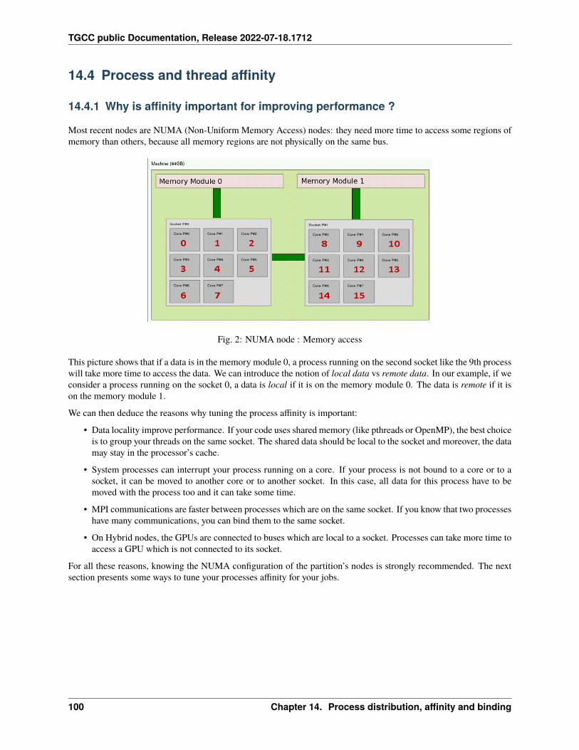
TGCC public Documentation, Release 2022-07-18.1712
14.4 Process and thread affinity
14.4.1 Why is affinity important for improving performance ?
Most recent nodes are NUMA (Non-Uniform Memory Access) nodes: they need more time to access some regions ofmemory than others, because all memory regions are not physically on the same bus.
Fig. 2: NUMA node : Memory access
This picture shows that if a data is in the memory module 0, a process running on the second socket like the 9th processwill take more time to access the data. We can introduce the notion of local data vs remote data. In our example, if weconsider a process running on the socket 0, a data is local if it is on the memory module 0. The data is remote if it ison the memory module 1.
We can then deduce the reasons why tuning the process affinity is important:
• Data locality improve performance. If your code uses shared memory (like pthreads or OpenMP), the best choiceis to group your threads on the same socket. The shared data should be local to the socket and moreover, the datamay stay in the processor’s cache.
• System processes can interrupt your process running on a core. If your process is not bound to a core or to asocket, it can be moved to another core or to another socket. In this case, all data for this process have to bemoved with the process too and it can take some time.
• MPI communications are faster between processes which are on the same socket. If you know that two processeshave many communications, you can bind them to the same socket.
• On Hybrid nodes, the GPUs are connected to buses which are local to a socket. Processes can take more time toaccess a GPU which is not connected to its socket.
For all these reasons, knowing the NUMA configuration of the partition’s nodes is strongly recommended. The nextsection presents some ways to tune your processes affinity for your jobs.
100 Chapter 14. Process distribution, affinity and binding
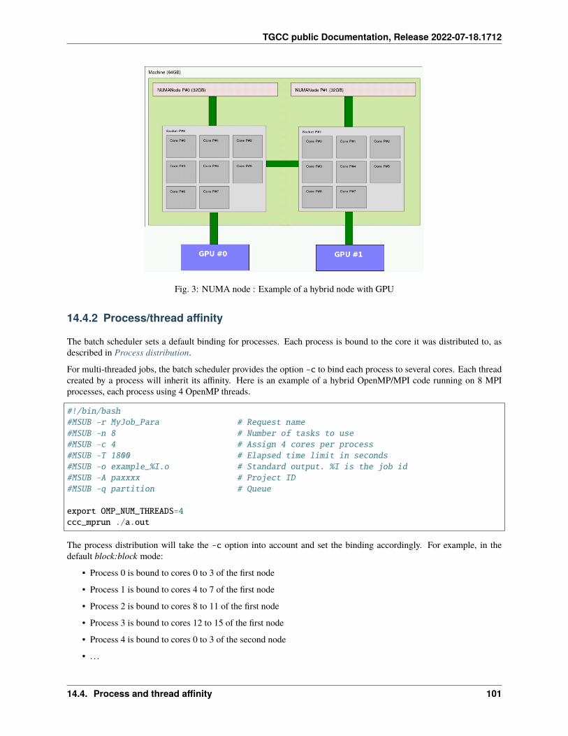
TGCC public Documentation, Release 2022-07-18.1712
Fig. 3: NUMA node : Example of a hybrid node with GPU
14.4.2 Process/thread affinity
The batch scheduler sets a default binding for processes. Each process is bound to the core it was distributed to, asdescribed in Process distribution.
For multi-threaded jobs, the batch scheduler provides the option -c to bind each process to several cores. Each threadcreated by a process will inherit its affinity. Here is an example of a hybrid OpenMP/MPI code running on 8 MPIprocesses, each process using 4 OpenMP threads.
#!/bin/bash#MSUB -r MyJob_Para # Request name#MSUB -n 8 # Number of tasks to use#MSUB -c 4 # Assign 4 cores per process#MSUB -T 1800 # Elapsed time limit in seconds#MSUB -o example_%I.o # Standard output. %I is the job id#MSUB -A paxxxx # Project ID#MSUB -q partition # Queue
export OMP_NUM_THREADS=4ccc_mprun ./a.out
The process distribution will take the -c option into account and set the binding accordingly. For example, in thedefault block:block mode:
• Process 0 is bound to cores 0 to 3 of the first node
• Process 1 is bound to cores 4 to 7 of the first node
• Process 2 is bound to cores 8 to 11 of the first node
• Process 3 is bound to cores 12 to 15 of the first node
• Process 4 is bound to cores 0 to 3 of the second node
• . . .
14.4. Process and thread affinity 101
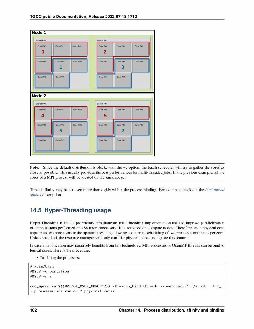
TGCC public Documentation, Release 2022-07-18.1712
Note: Since the default distribution is block, with the -c option, the batch scheduler will try to gather the cores asclose as possible. This usually provides the best performances for multi-threaded jobs. In the previous example, all thecores of a MPI process will be located on the same socket.
Thread affinity may be set even more thoroughly within the process binding. For example, check out the Intel threadaffinity description.
14.5 Hyper-Threading usage
Hyper-Threading is Intel’s proprietary simultaneous multithreading implementation used to improve parallelizationof computations performed on x86 microprocessors. It is activated on compute nodes. Therefore, each physical coreappears as two processors to the operating system, allowing concurrent scheduling of two processes or threads per core.Unless specified, the resource manager will only consider physical cores and ignore this feature.
In case an application may positively benefits from this technology, MPI processes or OpenMP threads can be bind tological cores. Here is the procedure:
• Doubling the processes:
#!/bin/bash#MSUB -q partition#MSUB -n 2
ccc_mprun -n $((BRIDGE_MSUB_NPROC*2)) -E'--cpu_bind=threads --overcommit' ./a.out # 4␣→˓processes are run on 2 physical cores
102 Chapter 14. Process distribution, affinity and binding
TGCC public Documentation, Release 2022-07-18.1712
• Doubling the threads:
#!/bin/bash#MSUB -q partition#MSUB -n 2#MSUB -c 8
export OMP_NUM_THREADS=$((BRIDGE_MSUB_NCORE*2)) # threads number must be equal to␣→˓logical coresccc_mprun ./a.out # each process runs 16 threads on 8 physical cores / 16 logical cores
14.6 Turbo
The processor turbo technology (Intel Turbo Boost or AMD turbo core) is available and activated by default on Irene.This technology dynamically adjusts CPU frequency in order to reach the highest frequency allowed by the availablepower and thermal limits. The Turbo can be responsible of performance variation because of hardware differencesbetween two nodes and if other jobs are running on the same node. One can choose to disable this technology byloading the module feature/system/turbo_off:
module load feature/system/turbo_off
Deactivating this technology allows a better control of the timing of the execution of the codes but can trigger poorperformances. One can choose to have capped performances by loading the feature feature/system/turbo_capped:
module load feature/system/turbo_capped
which sets the CPU frequency to a determined value which prevents Turbo to be activated for vectorized operations.
14.6. Turbo 103
TGCC public Documentation, Release 2022-07-18.1712
104 Chapter 14. Process distribution, affinity and binding
CHAPTER
FIFTEEN
PARALLEL IO
15.1 MPI-IO
MPI-IO provides a low level implementation of parallel I/O. It was introduced as a standard in MPI-2.
More information on how to use MPI-IO can be found in the I/O section of the official MPI documentation.
15.2 Recommended data usage on parallel file system
15.2.1 Technical considerations
On the computing center, parallel file systems are implemented with Lustre technology as follows:
• One MDS stores namespace metadata, such as file names, directories, access permissions, and file layout.
• Multiple OSSes (Object Storage Servers) store file data.
• Each supercomputer node is a client that accesses and uses the data.
When a file is opened or created:
1. Supercomputer node requests it to the MDS.
2. The MDS performs a hand-shake between the supercomputer node and the OSSes.
3. The node can now read and/or write directly by transferring data to the OSSes.
The important point is that all open, close and file name related calls from all the supercomputer nodes go to aunique server: the MDS.
These calls are often referred to as meta-data calls and too many of these calls can badly affect the overall performancesof the file system.
The following sections provide data usage guidelines to ensure the good operation of the parallel file systems.
105
TGCC public Documentation, Release 2022-07-18.1712
15.2.2 Big files vs small files
Lustre file system is optimized for bandwidth rather than latency.
• While manipulating small files, I/O performances are mainly latency-based (the hand-shakes with the MDS).
• While manipulating big files, latency impact is considerably reduced.
Thus, prefer having several big files instead of having many small files.
15.2.3 Number of files per directory
Many meta-data operations involve the MDS but also the OSSes.
Let us see with an example, a classic ls -l, what happens behind the scene:
1. Client asks the MDS to list all files in the current directory.
2. The MDS lists the names of the files (sub-directories, regular files, etc.).
3. The MDS knows everything about the sub-directories.
4. But MDS does not know the sizes of non-directory files (nor the date of last modification)!
5. So for each file the MDS synchronizes with each OSSes involved (sum of sizes, max of the date of modification,etc.).
Hence the more non-directory files you have within the directory, the slower the operation will be.
A similar scheme occurs to any file operation using stat system call for each file, like done with find or du commands.
This is the main reason why many file operations become slower as the number of regular files within a directoryincreases.
• As a consequence, it is strongly advised to have less than 10.000 files per directory.
• If you have more files, organize them into sub-directories (directories do not involve OSSes).
15.2.4 Files on STORE
STORE is a Lustre file systems linked to a Hierarchical Storage Management (HSM) relying on a magnetic tape storagesystem.
Thus they share the constraints of Lustre file systems and those of the magnetic tape storage.
Because tape storage has a long latency and the number of tape readers are limited, having big files becomes nearlymandatory.
That’s why in order to reduce the time of retrieval :
• each file should be bigger than 1GB (if needed, use tar to aggregate your small files)
• each file should be less than 1TB
When you can manipulate the file size (e.g. using tarball), making it around 100GB is recommended. Practicalexperience shows that a 100GB file is quick to retrieve with ccc_hsm get and subsequent manipulation or extractionis also fast.
You may use ccc_quota to check file size statistics on STORE (they are updated daily).
106 Chapter 15. Parallel IO
TGCC public Documentation, Release 2022-07-18.1712
15.2.5 Example of a good usage of filesystems
You have compiled your own program and installed it in your home directory under ~/products. In your home, yourprogram will be safe. Also, you may use some user defined modules that you would create in ~/products/modules/modulefiles as described in Extend your environment with modulefiles. It may simplify the use of your code. Toavoid reaching the quota limit on the home, don’t use it by default for any work. The best place to write submissionfiles and to launch your jobs would be the workdir. One of the advantages of the workdir is that it is shared betweencalculators. By launching your jobs from the workdir, you will be able to keep the submission scripts and the log files.Let us say the code generates lots of files, for example restart files, so that a new job can start where the last one stopped.In that case, the best is to launch the code on the scratchdir. It is the fastest and largest filesystem. However, data locatedon the scratchdir may be purged if they are not used for a while. Therefore, once your job ran successfully and youobtained the result files, you need to move them to an appropriate location if you want to keep them. That is the mainpurpose of the storedir. Once the job is finished, you can gather its result files in a big tar file that you shall copy on thestoredir.
So, a typical job would be launched from the workdir, where the submission scripts are located. The job would gothrough the following steps :
• Create a temporary directory on the scratchdir and go to this directory
• Untar large input files from the storedir to our directory in the scratchdir
• Launch the code
• Once it has finished running, check the results
• If the results are not needed at the moment for other runs, make a tar of the useful files and copy the tar on thestoredir
• Remove the temporary directory
Note that those steps are not compulsory and do not apply to every job. It is just one possible example of correct useof the different filesystems.
15.3 Parallel compression and decompression with pigz
Instead of using classical compression tools like gzip (included by default with tar), we recommend to use his parallelcounterpart pigz to get faster processing.
With this tool, we advise you to limit the number of threads used for compression between 4 and 8 to have a goodperformance / resources ratio. Increasing the number of threads should not dramatically improve performance andcould even slow your compression. To speed up the process you may also adjust the compression level at the cost ofreducing the compression quality. Decompression will be done by only one thread in any case and three more threadswill be used for various purposes (read, write, check).
Please do not use this tool on login nodes, and prefer an interactive submission with ccc_mprun -s or with a batchscript.
Compression and decompression example using 6 threads:
#!/bin/bash#MSUB -n 1#MSUB -c 6module load pigz
# compression:# we are forced to create a wrapper around pigz if we want to use
(continues on next page)
15.3. Parallel compression and decompression with pigz 107
TGCC public Documentation, Release 2022-07-18.1712
(continued from previous page)
# specific options to change the default behaviour of pigz.# Note that '$@' is important because tar can pass arguments to pigzcat <<EOF > pigz.sh#!/bin/bashpigz -p 6 \$@EOFchmod +x ./pigz.sh
tar -I ./pigz.sh -cf folder.tar.gz folder
# decompression:tar -I pigz -xf folder.tar.gz
For additional information, please refer to the man-pages of the software:
$ man pigz
108 Chapter 15. Parallel IO
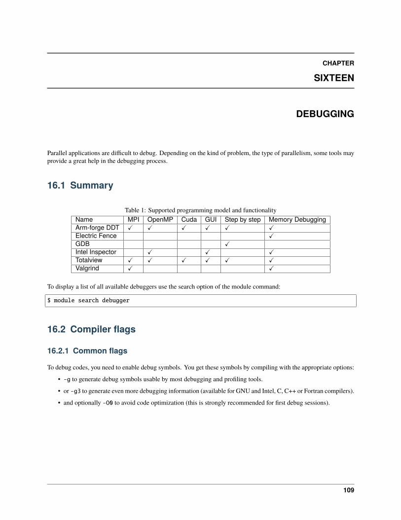
CHAPTER
SIXTEEN
DEBUGGING
Parallel applications are difficult to debug. Depending on the kind of problem, the type of parallelism, some tools mayprovide a great help in the debugging process.
16.1 Summary
Table 1: Supported programming model and functionalityName MPI OpenMP Cuda GUI Step by step Memory DebuggingArm-forge DDT X X X X X XElectric Fence XGDB XIntel Inspector X X XTotalview X X X X X XValgrind X X
To display a list of all available debuggers use the search option of the module command:
$ module search debugger
16.2 Compiler flags
16.2.1 Common flags
To debug codes, you need to enable debug symbols. You get these symbols by compiling with the appropriate options:
• -g to generate debug symbols usable by most debugging and profiling tools.
• or -g3 to generate even more debugging information (available for GNU and Intel, C, C++ or Fortran compilers).
• and optionally -O0 to avoid code optimization (this is strongly recommended for first debug sessions).
109
TGCC public Documentation, Release 2022-07-18.1712
16.2.2 Flags for Fortran
• -traceback with ifort or -fbacktrace with gfortran: specifies that a backtrace should be produced if theprogram crashes, showing which functions or subroutines were being called when the error occurs.
For example, when getting a segmentation fault in Fortran, you may get the following error message which is not veryuseful:
forrtl: severe (174): SIGSEGV, segmentation fault occurredImage PC Routine Line Sourcerun_exe 000000010005EAC7 Unknown Unknown Unknownrun_exe 000000010005DDA9 Unknown Unknown Unknownrun_exe 00000001000009BC Unknown Unknown Unknownrun_exe 0000000100000954 Unknown Unknown Unknown
A code compiled with -fbacktrace or -traceback will give a more relevant output:
forrtl: severe (174): SIGSEGV, segmentation fault occurredImage PC Routine Line Sourcerun_exe 000000010005EAC7 test_m_ 265 mod_test.f90run_exe 000000010005DDA9 io_ 52 io.f90run_exe 00000001000009BC setup_ 65 test_Setup.f90run_exe 0000000100000954 main_ 110 launch.f90
• -check bounds with ifort or -fbounds-check with gfortran: checks that an index is within the boundsof the array each time an array element is accessed. This option is expected to substantially slow down programexecution but is a convenient way to track down bugs related to arrays. Without this flag, an illegal array accesswould produce either a subtle error that might not become apparent until much later in the program or will causean immediate segmentation fault with poor information on the origin of the error.
Note: Be careful. Most of these compiler options will slow down your code performances.
16.3 Available debuggers
• GDB: The GNU Project Debugger
• DDT: Arm-forge Distributed Debugging Tool
• TotalView: RogueWave TotalView Graphical Debugger
16.3.1 GDB
GDB is the Gnu DeBugger. It is a lightweight simple serial debugger available on most systems.
To start a program under GDB, first make sure it is compiled with -g. Start a GDB session for your code:
$ gdb ./gdb_testGNU gdb (GDB) Red Hat Enterprise LinuxCopyright (C) 2010 Free Software Foundation, Inc.(gdb)
Once the GDB session is started, launch the code with:
110 Chapter 16. Debugging
TGCC public Documentation, Release 2022-07-18.1712
(gdb) run
If an error occurs, you will be able to get information with backtrace:
Program received signal SIGSEGV, Segmentation fault.(gdb) backtrace#0 0x00000000004005e0 in func1 (rank=1) at test.c:14#1 0x0000000000400667 in main (argc=1, argv=0x7fffffffacc8) at test.c:30
GDB allows to set breakpoints, run the code step by step and more. See man gdb for more information and options.
Note: GDB only works for serial code. For parallel programs, other tools are available such as Arm-forge DDT andTotalview.
16.3.2 DDT
DDT is a highly scalable debugger specifically adapted to supercomputers.
Basics
You can use DDT after loading the appropriate module:
$ module load arm-forge
Then use the command ddt. For parallel codes, edit your submission script and replace the line
$ ccc_mprun -n 16 ./a.out
with:
$ ddt -n 16 ./a.out
You may want to add the -noqueue option to make sure DDT will not submit a new job to the scheduler. You haveto specify the good version of the mpi distribution by selecting run and select SLURM (generic) implementation asshown on the figures below.
Example of submission script:
$ cat ddt.job#!/bin/bash#MSUB -r MyJob_Para # Request name#MSUB -q partition # Queue#MSUB -n 32 # Number of tasks to use#MSUB -T 1800 # Elapsed time limit in seconds#MSUB -o example_%I.o # Standard output. %I is the job id#MSUB -e example_%I.e # Error output. %I is the job idset -xcd ${BRIDGE_MSUB_PWD}ddt -n 32 ./ddt_test
$ ccc_msub -X ddt.job
16.3. Available debuggers 111
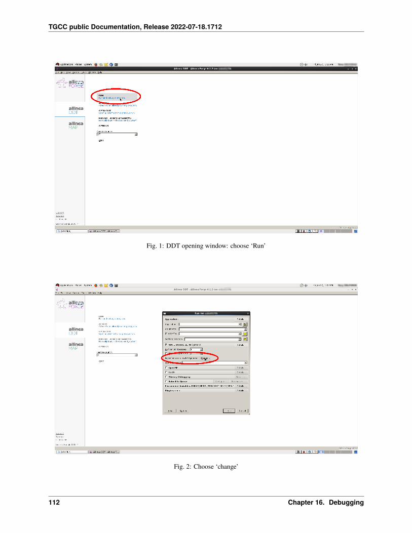
TGCC public Documentation, Release 2022-07-18.1712
Fig. 1: DDT opening window: choose ‘Run’
Fig. 2: Choose ‘change’
112 Chapter 16. Debugging
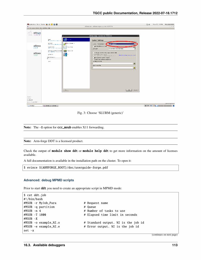
TGCC public Documentation, Release 2022-07-18.1712
Fig. 3: Choose ‘SLURM (generic)’
Note: The -X option for ccc_msub enables X11 forwarding.
Note: Arm-forge DDT is a licensed product.
Check the output of module show ddt or module help ddt to get more information on the amount of licensesavailable.
A full documentation is available in the installation path on the cluster. To open it:
$ evince ${ARMFORGE_ROOT}/doc/userguide-forge.pdf
Advanced: debug MPMD scripts
Prior to start ddt you need to create an appropriate script in MPMD mode:
$ cat ddt.job#!/bin/bash#MSUB -r MyJob_Para # Request name#MSUB -q partition # Queue#MSUB -n 4 # Number of tasks to use#MSUB -T 1800 # Elapsed time limit in seconds#MSUB -X#MSUB -o example_%I.o # Standard output. %I is the job id#MSUB -e example_%I.e # Error output. %I is the job idset -x
(continues on next page)
16.3. Available debuggers 113
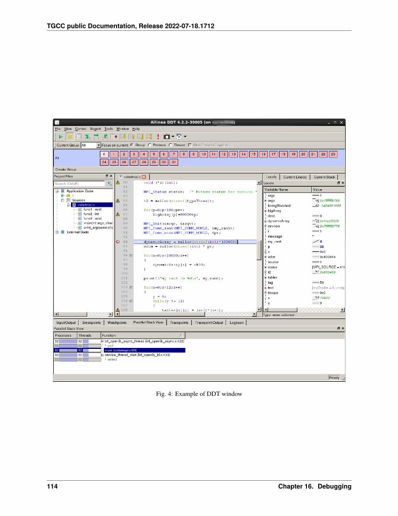
TGCC public Documentation, Release 2022-07-18.1712
Fig. 4: Example of DDT window
114 Chapter 16. Debugging
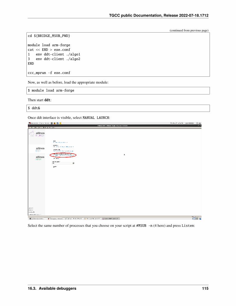
TGCC public Documentation, Release 2022-07-18.1712
(continued from previous page)
cd ${BRIDGE_MSUB_PWD}
module load arm-forgecat << END > exe.conf1 env ddt-client ./algo13 env ddt-client ./algo2END
ccc_mprun -f exe.conf
Now, as well as before, load the appropriate module:
$ module load arm-forge
Then start ddt:
$ ddt&
Once ddt interface is visible, select MANUAL LAUNCH:
Select the same number of processes that you choose on your script at #MSUB -n (4 here) and press Listen:
16.3. Available debuggers 115
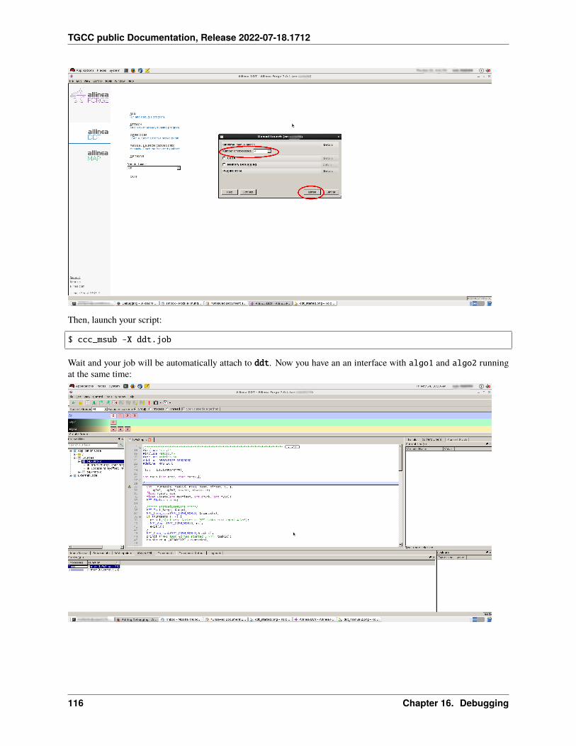
TGCC public Documentation, Release 2022-07-18.1712
Then, launch your script:
$ ccc_msub -X ddt.job
Wait and your job will be automatically attach to ddt. Now you have an an interface with algo1 and algo2 runningat the same time:
116 Chapter 16. Debugging
TGCC public Documentation, Release 2022-07-18.1712
16.3.3 TotalView
TotalView may be used by loading a module and by submitting an appropriate job:
$ module load totalview
Then launch your job with a submission script like:
#!/bin/bash#MSUB -r MyJob # Request name#MSUB -q partition # Queue#MSUB -n 8 # Number of tasks to use#MSUB -T 600#MSUB -o totalview_%I.o # Standard output. %I is the job id#MSUB -e totalview_%I.e # Error output. %I is the job idset -xcd ${BRIDGE_MSUB_PWD}ccc_mprun -d tv ./totalview_test
It needs to be submitted with:
$ ccc_msub -X totalview.job
Totalview should open on the Startup Parameters window. There is nothing to change here, just hit OK. Once in themain window, you can either come back to the parameter window with “<ctrl-a>” or launch the code with “g”.
Note: Totalview is a licensed product.
Check the output of module show totalview or module help totalview to get more information on the amountof licenses available.
A full documentation is available in the installation path on the cluster. To open it:
$ evince ${TOTALVIEW_ROOT}/doc/pdf/TotalView_User_Guide.pdf
16.4 Other tools
16.4.1 Valgrind Memcheck
Valgrind is an instrumentation framework for dynamic analysis tools. It comes with a set of tools for profiling anddebugging.
Memcheck is a memory error detector. It is the default use of Valgrind so any call to valgrind is equivalent to calling
$ valgrind --tools=memcheck
To check your code with Valgrind, just call valgrind before the program :
$ module load valgrind$ valgrind ./test
16.4. Other tools 117
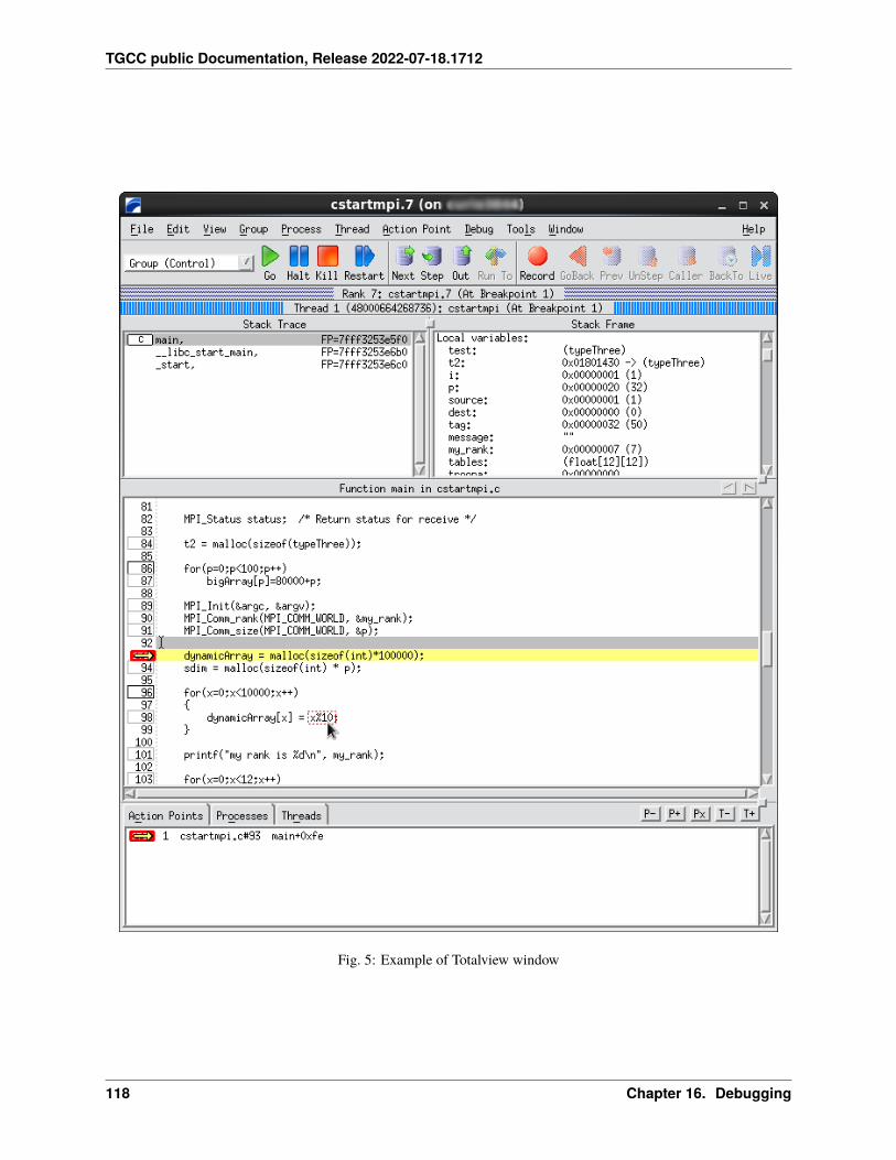
TGCC public Documentation, Release 2022-07-18.1712
Fig. 5: Example of Totalview window
118 Chapter 16. Debugging
TGCC public Documentation, Release 2022-07-18.1712
To run MPI programs under Valgrind, use the available library “libmpiwrap” to filter false positives on MPI functions.It is available through the VALGRIND_PRELOAD environment variable. It is also possible to specify the output file andto force Valgrind to output one file per process (with --log-file)
#!/bin/bash#MSUB -n 32#MSUB -T 1800#MSUB -q partition
module load valgrind
export LD_PRELOAD=${VALGRIND_PRELOAD}
ccc_mprun valgrind --log-file=valgrind_%q{SLURM_JOBID}_%q{SLURM_PROCID} ./test
Here is the kind of output Valgrind returns :
==22860== Invalid write of size 4==22860== at 0x4005DD: func1 (test1.c:12)==22860== by 0x40061E: main (test1.c:20)==22860== Address 0x4c11068 is 0 bytes after a block of size 40 alloc'd==22860== at 0x4A05FDE: malloc (vg_replace_malloc.c:236)==22860== by 0x4005B0: func1 (test1.c:9)==22860== by 0x40061E: main (test1.c:20)
16.4.2 Electric Fence
Electric Fence helps you detect two common programming bugs: software that overruns the boundaries of a malloc()memory allocation, and software that touches a memory allocation that has been released by free(). Those errors do notalways lead to a crash but may cause some unexpected behavior. Running your program with Electric Fence will forcea segmentation fault (SIGSEGV) when any of these errors are detected, thus helping to detect the offending instruction.
The Electric Fence library can be loaded at runtime through LD_PRELOAD:
$ module load electricfence$ export LD_PRELOAD=${EF_PRELOAD}$ ./a.out
The best way to proceed if a segfault occurs is to combine the use of Electric Fence with a debugger.
Note: For parallel codes launched with ccc_mprun, the LD_PRELOAD does not need to be modified, just loading themodule is enough.
16.4. Other tools 119
TGCC public Documentation, Release 2022-07-18.1712
16.4.3 Intel Inspector
Inspector is a memory and thread debugger developed by Intel which aim to help debug OpenMP programs. Becauseof the notion of shared memory, multi-threading comes with its own, very specific bugs. Intel Inspector will detect anydeadlock or memory concurrency which will be hightlighted and identified in the source code via the GUI (GraphicUser Interface).
To use it, you need to load the corresponding module as follow:
$ module load inspector
Information is collected by launching the code with the command line tool. It needs to be done in a submission script oran interactive session. Never on the login nodes. There are two different analyse types characterized by three levels eachwhich define the degree of the analysis and so the associated overhead (The highest level is most expensive consumerof time) :
• Memory analysis:
– mi1 : Detect Leaks
– mi2 : Detect Memory Problems
– mi3 : Locate Memory Problems
• Threading error analysis
– ti1 : Detect Deadlocks
– ti2 : Detect Deadlocks and Data Races
– ti3 : Locate Deadlocks and Data Races
Information analyse type and options are available under the command inspxe-cl -help collect
To launch the collection please proceed as follow :
Submission script example:
#MSUB -r insp_code#MSUB -q partition#MSUB -n 28 # Number of task#MSUB -c 1 # Number of core per task#MSUB -o inspe_code_%J.e # Error output#MSUB -e inspe_code_%J.o # Output#MSUB -xccc_mprun inspxe-cl -r mybinary_mi1 -collect mi1 -knob detect-leaks-on-exit=true -knob␣→˓enable-memory-growth-detection=false -knob enable-on-demand-leak-detection=false -knob␣→˓still-allocated-memory=true -knob stack-depth=8 -module-filter-mode=include -→˓appdebug=off -no-trace-mpi -app-working-dir $PWD -- ./a.out #Do not forget the -r␣→˓option
Once the collection is done, a file *.inspxe should be created. Open it under the Intel Inspector GUI, preferably inan interactive session with X11 forwarding or with Remote Desktop session as follow:
Launch the gui:
$inspxe-gui
Select Open Result
Open the collected Data.
120 Chapter 16. Debugging
TGCC public Documentation, Release 2022-07-18.1712
Fig. 6: command line
Fig. 7: collected data
16.4. Other tools 121
TGCC public Documentation, Release 2022-07-18.1712
Then fix your code.
Tips:
To simply get the appropriate command line to launch, please proceed as follow.
First, launch inspector gui (-XY is needed).
$ inspxe-gui
Create a new project:
Fig. 8: New project
Create a new analyse:
Select the analyse type
Get the comand line:
For more information, see the full Intel Inspector Documentation.
122 Chapter 16. Debugging
TGCC public Documentation, Release 2022-07-18.1712
Fig. 9: New analysis
Fig. 10: analysis type
16.4. Other tools 123
TGCC public Documentation, Release 2022-07-18.1712
Fig. 11: command line
124 Chapter 16. Debugging
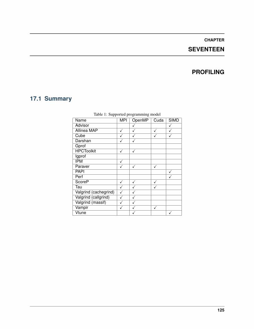
CHAPTER
SEVENTEEN
PROFILING
17.1 Summary
Table 1: Supported programming modelName MPI OpenMP Cuda SIMDAdvisor X XAllinea MAP X X X XCube X X X XDarshan X XGprofHPCToolkit X XIgprofIPM XParaver X X XPAPI XPerf XScoreP X X XTau X X XValgrind (cachegrind) X XValgrind (callgrind) X XValgrind (massif) X XVampir X X XVtune X X
125

TGCC public Documentation, Release 2022-07-18.1712
Table 2: Collectible eventsName Comm I/O Call
graphHardware coun-ters
Memory us-age
Cache us-age
Advisor XAllinea MAP X X XCube X X XDarshan XGprof XHPCToolkit X X XIgprof XIPM X XParaver X XPAPI X X XPerf X X X X XScoreP X X X X XTau X X X XValgrind(cachegrind)
X
Valgrind (callgrind) XValgrind (massif) XVampir XVtune X X
Table 3: Tool support and type of profilingName Collection GUI Sampling Tracing Instrumentation necessaryAdvisor X X XAllinea MAP X X X XCube X X X XDarshan X XGprof X X X XHPCToolkit X X X XIgprof X X XIPM X XParaver X X XPAPI X X XPerf XScoreP X X X XTau X X X XValgrind (cachegrind) X XValgrind (callgrind) X XValgrind (massif) X XVampir X X XVtune X X X
To display a list of all available profilers use the search option of the module command :
126 Chapter 17. Profiling
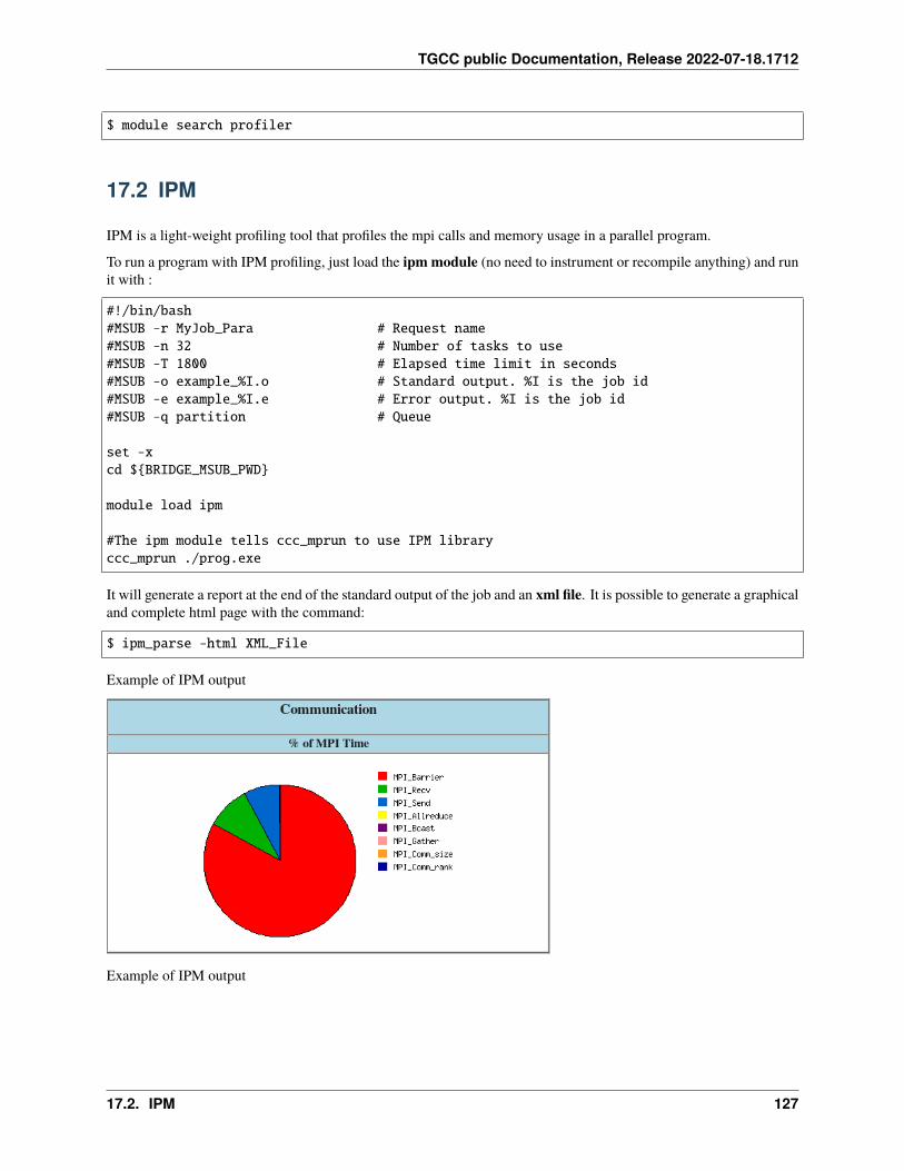
TGCC public Documentation, Release 2022-07-18.1712
$ module search profiler
17.2 IPM
IPM is a light-weight profiling tool that profiles the mpi calls and memory usage in a parallel program.
To run a program with IPM profiling, just load the ipm module (no need to instrument or recompile anything) and runit with :
#!/bin/bash#MSUB -r MyJob_Para # Request name#MSUB -n 32 # Number of tasks to use#MSUB -T 1800 # Elapsed time limit in seconds#MSUB -o example_%I.o # Standard output. %I is the job id#MSUB -e example_%I.e # Error output. %I is the job id#MSUB -q partition # Queue
set -xcd ${BRIDGE_MSUB_PWD}
module load ipm
#The ipm module tells ccc_mprun to use IPM libraryccc_mprun ./prog.exe
It will generate a report at the end of the standard output of the job and an xml file. It is possible to generate a graphicaland complete html page with the command:
$ ipm_parse -html XML_File
Example of IPM output
Example of IPM output
17.2. IPM 127
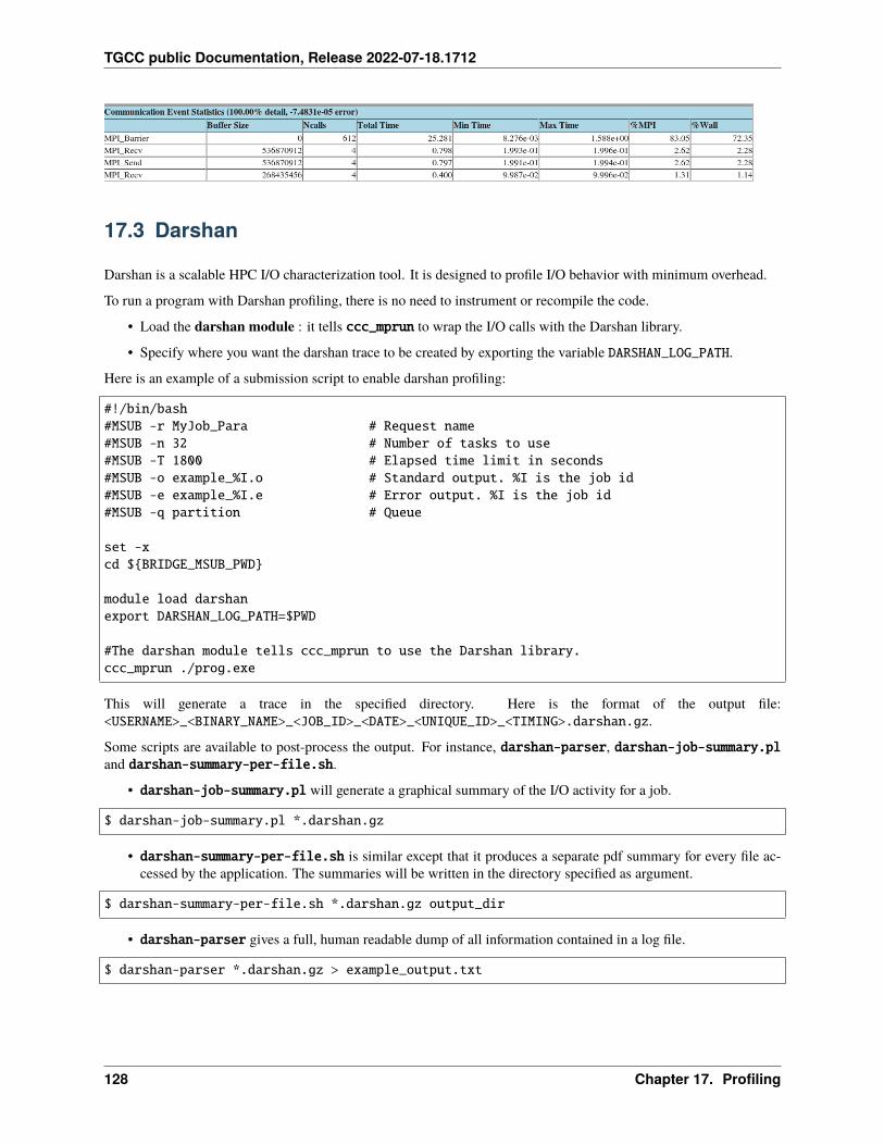
TGCC public Documentation, Release 2022-07-18.1712
17.3 Darshan
Darshan is a scalable HPC I/O characterization tool. It is designed to profile I/O behavior with minimum overhead.
To run a program with Darshan profiling, there is no need to instrument or recompile the code.
• Load the darshan module : it tells ccc_mprun to wrap the I/O calls with the Darshan library.
• Specify where you want the darshan trace to be created by exporting the variable DARSHAN_LOG_PATH.
Here is an example of a submission script to enable darshan profiling:
#!/bin/bash#MSUB -r MyJob_Para # Request name#MSUB -n 32 # Number of tasks to use#MSUB -T 1800 # Elapsed time limit in seconds#MSUB -o example_%I.o # Standard output. %I is the job id#MSUB -e example_%I.e # Error output. %I is the job id#MSUB -q partition # Queue
set -xcd ${BRIDGE_MSUB_PWD}
module load darshanexport DARSHAN_LOG_PATH=$PWD
#The darshan module tells ccc_mprun to use the Darshan library.ccc_mprun ./prog.exe
This will generate a trace in the specified directory. Here is the format of the output file:<USERNAME>_<BINARY_NAME>_<JOB_ID>_<DATE>_<UNIQUE_ID>_<TIMING>.darshan.gz.
Some scripts are available to post-process the output. For instance, darshan-parser, darshan-job-summary.pland darshan-summary-per-file.sh.
• darshan-job-summary.pl will generate a graphical summary of the I/O activity for a job.
$ darshan-job-summary.pl *.darshan.gz
• darshan-summary-per-file.sh is similar except that it produces a separate pdf summary for every file ac-cessed by the application. The summaries will be written in the directory specified as argument.
$ darshan-summary-per-file.sh *.darshan.gz output_dir
• darshan-parser gives a full, human readable dump of all information contained in a log file.
$ darshan-parser *.darshan.gz > example_output.txt
128 Chapter 17. Profiling
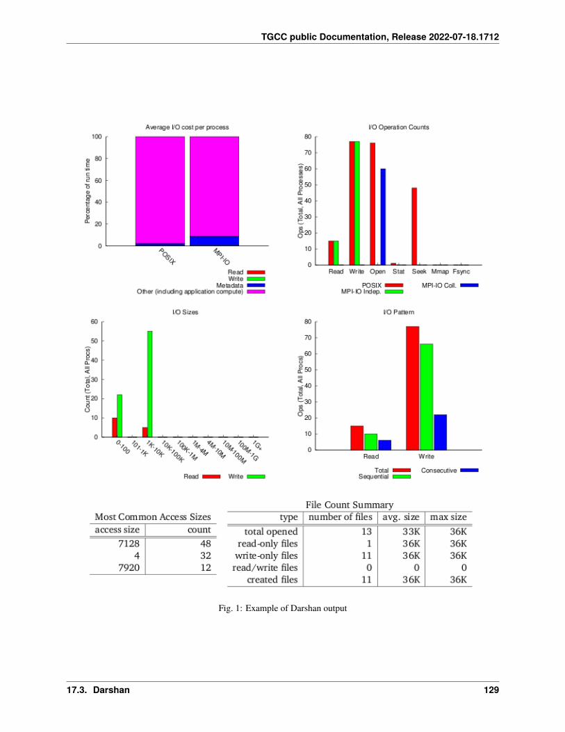
TGCC public Documentation, Release 2022-07-18.1712
Fig. 1: Example of Darshan output
17.3. Darshan 129
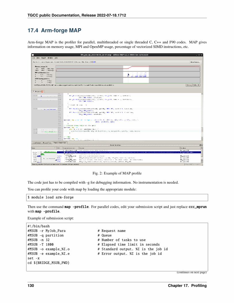
TGCC public Documentation, Release 2022-07-18.1712
17.4 Arm-forge MAP
Arm-forge MAP is the profiler for parallel, multithreaded or single threaded C, C++ and F90 codes. MAP givesinformation on memory usage, MPI and OpenMP usage, percentage of vectorized SIMD instructions, etc.
Fig. 2: Example of MAP profile
The code just has to be compiled with -g for debugging information. No instrumentation is needed.
You can profile your code with map by loading the appropriate module:
$ module load arm-forge
Then use the command map -profile. For parallel codes, edit your submission script and just replace ccc_mprunwith map -profile.
Example of submission script:
#!/bin/bash#MSUB -r MyJob_Para # Request name#MSUB -q partition # Queue#MSUB -n 32 # Number of tasks to use#MSUB -T 1800 # Elapsed time limit in seconds#MSUB -o example_%I.o # Standard output. %I is the job id#MSUB -e example_%I.e # Error output. %I is the job idset -xcd ${BRIDGE_MSUB_PWD}
(continues on next page)
130 Chapter 17. Profiling
TGCC public Documentation, Release 2022-07-18.1712
(continued from previous page)
module load arm-forgemap -n 32 ./a.out
Once the job has finished, a .map file should have been created. It can be opened from a remote desktop session orfrom an interactive session with the following command:
$ map <output_name>.map
Note: Arm-forge MAP is a licenced product.
Check the output of module show arm-forge or module help arm-forge to get more information on the amountof licences available.
A full documentation is available in the installation path on the cluster. To open it:
$ evince ${MAP_ROOT}/doc/userguide-forge.pdf
17.5 Gprof
Gprof produces an execution profile of C/C++ and Fortran programs. The effect of called routines is incorporated inthe profile of each caller. The profile data is taken from the call graph profile file (gmon.out default) which is created byprograms that are compiled with the -pg option. Gprof reads the given object file (the default is “a.out”) and establishesthe relation between its symbol table and the call graph profile from gmon.out.
• To load gprof
$ module load gprof
• To compile with -pg option
$ icc -pg hello.c
• If your application is MPI, set environment variable to rename gmon files and enable one file per process
$ export GMON_OUT_PREFIX='gmon.out-'`/bin/uname -n`
Files generated will be named gmon.out-<hostname>.<pid> (ie: gmon.out-node1192.56893).
• To generate call graph profile gmon.out
$ ./a.out
• To display flat profile and call graph
$ gprof a.out gmon.out
• To display only the flat profile
$ gprof -p -b ./a.out gmon.out
Flat profile:(continues on next page)
17.5. Gprof 131
TGCC public Documentation, Release 2022-07-18.1712
(continued from previous page)
Each sample counts as 0.01 seconds.% cumulative self self totaltime seconds seconds calls s/call s/call name67.72 10.24 10.24 1 10.24 10.24 bar33.06 15.24 5.00 main0.00 15.24 0.00 1 0.00 10.24 foo
• To display the flat profile of one specific routine
$ gprof -p<routine> -b ./a.out gmon.out
• To display only the call graph
$ gprof -q -b ./a.out gmon.out
Call graph (explanation follows)index % time self children called name
<spontaneous>[1] 100.0 5.00 10.24 main [1]
0.00 10.24 1/1 foo [3]-----------------------------------------------
10.24 0.00 1/1 foo [3][2] 67.2 10.24 0.00 1 bar [2]-----------------------------------------------
0.00 10.24 1/1 main [1][3] 67.2 0.00 10.24 1 foo [3]
10.24 0.00 1/1 bar [2]-----------------------------------------------
• To display the call graph of one specific routine
$ gprof -q<routine> -b ./a.out gmon.out
• To generate a graph from data, see gprof2dot and gprof
17.6 igprof
IgProf is a tool for measuring and analysing application memory and performance characteristics. To run a programwith IgProf profiling, there is no need to instrument or recompile the code.
• To load igprof
module load igprof
• To generate the memory trace
igprof -d -mp -z -o igprof.mp.gz myApp [arg1 arg2 ...] >& igtest.mp.log
• To see unfreed memory, extract the MEM_LIVE report from the memory trace with:
igprof-analyse -d -v -g -r MEM_LIVE igprof.mp.gz > igreport_live.res
132 Chapter 17. Profiling
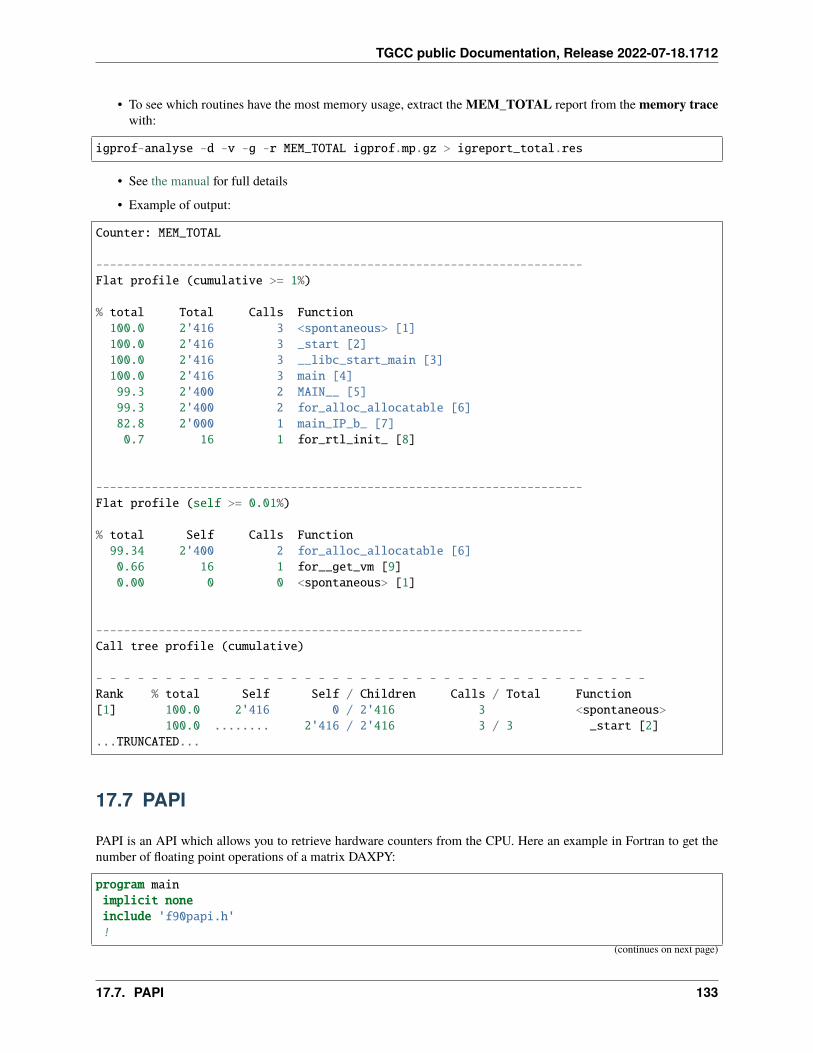
TGCC public Documentation, Release 2022-07-18.1712
• To see which routines have the most memory usage, extract the MEM_TOTAL report from the memory tracewith:
igprof-analyse -d -v -g -r MEM_TOTAL igprof.mp.gz > igreport_total.res
• See the manual for full details
• Example of output:
Counter: MEM_TOTAL
----------------------------------------------------------------------Flat profile (cumulative >= 1%)
% total Total Calls Function100.0 2'416 3 <spontaneous> [1]100.0 2'416 3 _start [2]100.0 2'416 3 __libc_start_main [3]100.0 2'416 3 main [4]99.3 2'400 2 MAIN__ [5]99.3 2'400 2 for_alloc_allocatable [6]82.8 2'000 1 main_IP_b_ [7]0.7 16 1 for_rtl_init_ [8]
----------------------------------------------------------------------Flat profile (self >= 0.01%)
% total Self Calls Function99.34 2'400 2 for_alloc_allocatable [6]0.66 16 1 for__get_vm [9]0.00 0 0 <spontaneous> [1]
----------------------------------------------------------------------Call tree profile (cumulative)
- - - - - - - - - - - - - - - - - - - - - - - - - - - - - - - - - - - - - - - -Rank % total Self Self / Children Calls / Total Function[1] 100.0 2'416 0 / 2'416 3 <spontaneous>
100.0 ........ 2'416 / 2'416 3 / 3 _start [2]...TRUNCATED...
17.7 PAPI
PAPI is an API which allows you to retrieve hardware counters from the CPU. Here an example in Fortran to get thenumber of floating point operations of a matrix DAXPY:
program mainimplicit noneinclude 'f90papi.h'!
(continues on next page)
17.7. PAPI 133
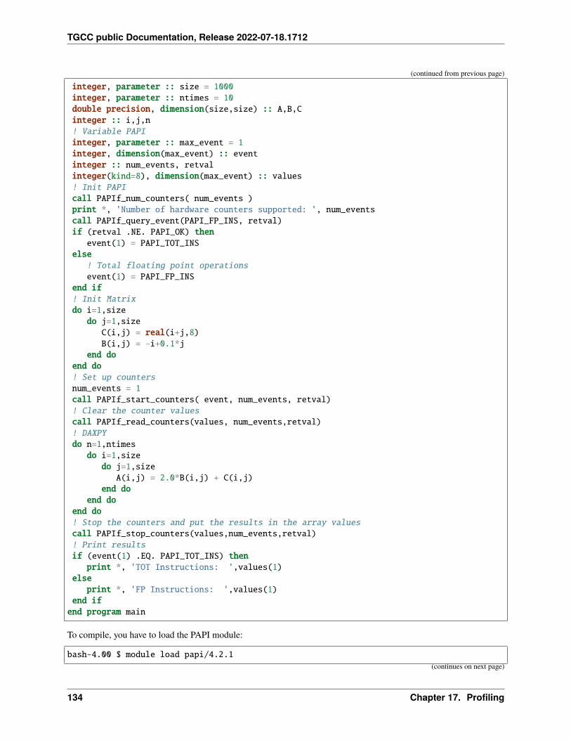
TGCC public Documentation, Release 2022-07-18.1712
(continued from previous page)
integer, parameter :: size = 1000integer, parameter :: ntimes = 10double precision, dimension(size,size) :: A,B,Cinteger :: i,j,n! Variable PAPIinteger, parameter :: max_event = 1integer, dimension(max_event) :: eventinteger :: num_events, retvalinteger(kind=8), dimension(max_event) :: values! Init PAPIcall PAPIf_num_counters( num_events )print *, 'Number of hardware counters supported: ', num_eventscall PAPIf_query_event(PAPI_FP_INS, retval)if (retval .NE. PAPI_OK) then
event(1) = PAPI_TOT_INSelse! Total floating point operationsevent(1) = PAPI_FP_INS
end if! Init Matrixdo i=1,sizedo j=1,size
C(i,j) = real(i+j,8)B(i,j) = -i+0.1*j
end doend do! Set up countersnum_events = 1call PAPIf_start_counters( event, num_events, retval)! Clear the counter valuescall PAPIf_read_counters(values, num_events,retval)! DAXPYdo n=1,ntimesdo i=1,sizedo j=1,size
A(i,j) = 2.0*B(i,j) + C(i,j)end do
end doend do! Stop the counters and put the results in the array valuescall PAPIf_stop_counters(values,num_events,retval)! Print resultsif (event(1) .EQ. PAPI_TOT_INS) thenprint *, 'TOT Instructions: ',values(1)
elseprint *, 'FP Instructions: ',values(1)
end ifend program main
To compile, you have to load the PAPI module:
bash-4.00 $ module load papi/4.2.1(continues on next page)
134 Chapter 17. Profiling
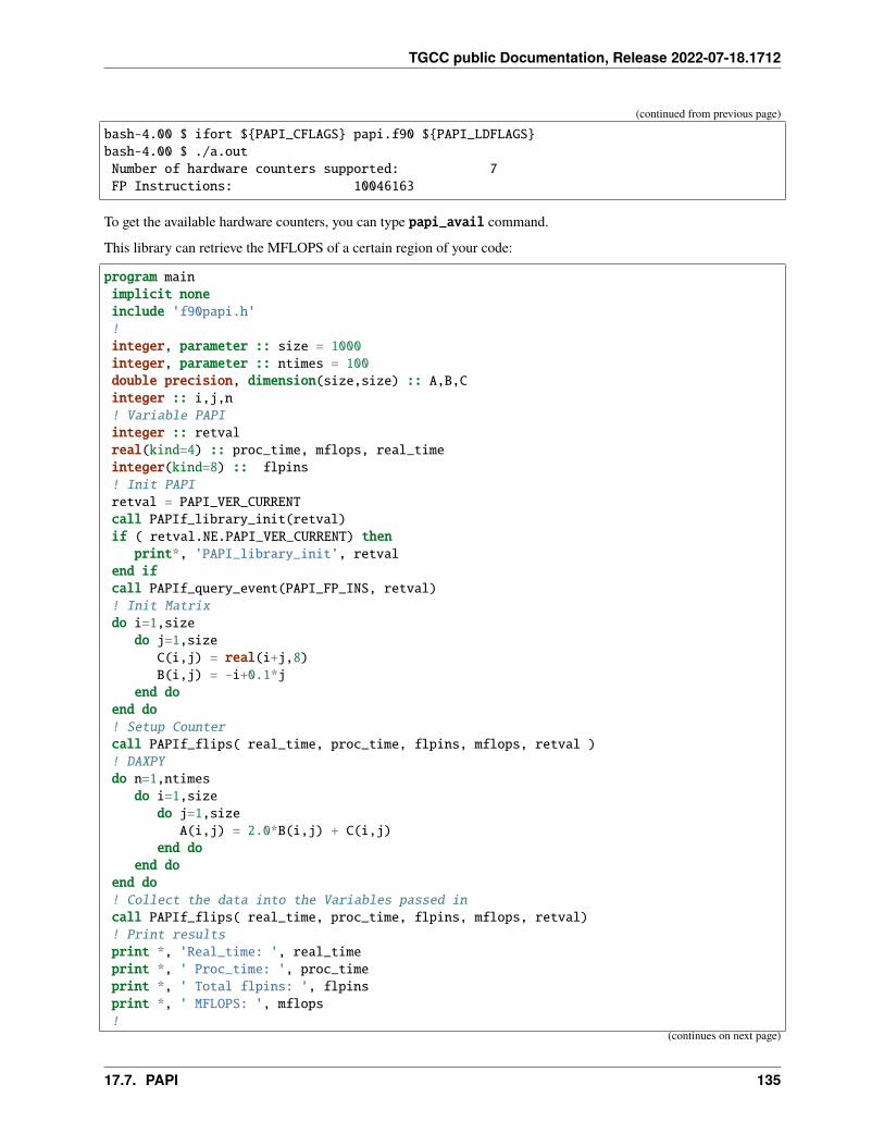
TGCC public Documentation, Release 2022-07-18.1712
(continued from previous page)
bash-4.00 $ ifort ${PAPI_CFLAGS} papi.f90 ${PAPI_LDFLAGS}bash-4.00 $ ./a.outNumber of hardware counters supported: 7FP Instructions: 10046163
To get the available hardware counters, you can type papi_avail command.
This library can retrieve the MFLOPS of a certain region of your code:
program mainimplicit noneinclude 'f90papi.h'!integer, parameter :: size = 1000integer, parameter :: ntimes = 100double precision, dimension(size,size) :: A,B,Cinteger :: i,j,n! Variable PAPIinteger :: retvalreal(kind=4) :: proc_time, mflops, real_timeinteger(kind=8) :: flpins! Init PAPIretval = PAPI_VER_CURRENTcall PAPIf_library_init(retval)if ( retval.NE.PAPI_VER_CURRENT) thenprint*, 'PAPI_library_init', retval
end ifcall PAPIf_query_event(PAPI_FP_INS, retval)! Init Matrixdo i=1,sizedo j=1,size
C(i,j) = real(i+j,8)B(i,j) = -i+0.1*j
end doend do! Setup Countercall PAPIf_flips( real_time, proc_time, flpins, mflops, retval )! DAXPYdo n=1,ntimesdo i=1,sizedo j=1,size
A(i,j) = 2.0*B(i,j) + C(i,j)end do
end doend do! Collect the data into the Variables passed incall PAPIf_flips( real_time, proc_time, flpins, mflops, retval)! Print resultsprint *, 'Real_time: ', real_timeprint *, ' Proc_time: ', proc_timeprint *, ' Total flpins: ', flpinsprint *, ' MFLOPS: ', mflops!
(continues on next page)
17.7. PAPI 135
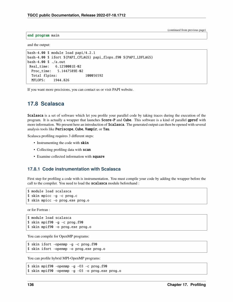
TGCC public Documentation, Release 2022-07-18.1712
(continued from previous page)
end program main
and the output:
bash-4.00 $ module load papi/4.2.1bash-4.00 $ ifort ${PAPI_CFLAGS} papi_flops.f90 ${PAPI_LDFLAGS}bash-4.00 $ ./a.outReal_time: 6.1250001E-02Proc_time: 5.1447589E-02Total flpins: 100056592MFLOPS: 1944.826
If you want more precisions, you can contact us or visit PAPI website.
17.8 Scalasca
Scalasca is a set of software which let you profile your parallel code by taking traces during the execution of theprogram. It is actually a wrapper that launches Score-P and Cube. This software is a kind of parallel gprof withmore information. We present here an introduction of Scalasca. The generated output can then be opened with severalanalysis tools like Periscope, Cube, Vampir, or Tau.
Scalasca profiling requires 3 different steps:
• Instrumenting the code with skin
• Collecting profiling data with scan
• Examine collected information with square
17.8.1 Code instrumentation with Scalasca
First step for profiling a code with is instrumentation. You must compile your code by adding the wrapper before thecall to the compiler. You need to load the scalasca module beforehand :
$ module load scalasca$ skin mpicc -g -c prog.c$ skin mpicc -o prog.exe prog.o
or for Fortran :
$ module load scalasca$ skin mpif90 -g -c prog.f90$ skin mpif90 -o prog.exe prog.o
You can compile for OpenMP programs:
$ skin ifort -openmp -g -c prog.f90$ skin ifort -openmp -o prog.exe prog.o
You can profile hybrid MPI-OpenMP programs:
$ skin mpif90 -openmp -g -O3 -c prog.f90$ skin mpif90 -openmp -g -O3 -o prog.exe prog.o
136 Chapter 17. Profiling
TGCC public Documentation, Release 2022-07-18.1712
17.8.2 Simple profiling with Scalasca
Once the code has been instrumented with Scalasca, run it with scan. By default, a simple summary profile isgenerated.
Here is a simple example of a submission script:
#!/bin/bash#MSUB -r MyJob_Para # Request name#MSUB -n 32 # Number of tasks to use#MSUB -T 1800 # Elapsed time limit in seconds#MSUB -o example_%I.o # Standard output. %I is the job id#MSUB -e example_%I.e # Error output. %I is the job id#MSUB -q partition # Queue
set -xcd ${BRIDGE_MSUB_PWD}
module load scalascaexport SCOREP_EXPERIMENT_DIRECTORY=scorep_profile.${BRIDGE_MSUB_JOBID}scan ccc_mprun ./prog.exe
At the end of execution, the program generates a directory which contains the profiling files (the directory name ischosen with the SCOREP_EXPERIMENT_DIRECTORY environment variable):
$ tree scorep_profile.2871901|- profile.cubex`- scorep.cfg
The profile information can then be visualized with square:
$ module load scalasca$ square scorep_profile.2871901
17.8.3 Scalasca with PAPI
Score-P can retrieve the hardware counter with PAPI. For example, if you want retrieve the number of floating pointoperations:
#!/bin/bash#MSUB -r MyJob_Para # Request name#MSUB -n 32 # Number of tasks to use#MSUB -T 1800 # Elapsed time limit in seconds#MSUB -o example_%I.o # Standard output. %I is the job id#MSUB -e example_%I.e # Error output. %I is the job id#MSUB -q partition # Queue
set -xcd ${BRIDGE_MSUB_PWD}
module load scalascaexport SCOREP_EXPERIMENT_DIRECTORY=scorep_profile.${BRIDGE_MSUB_JOBID}
(continues on next page)
17.8. Scalasca 137
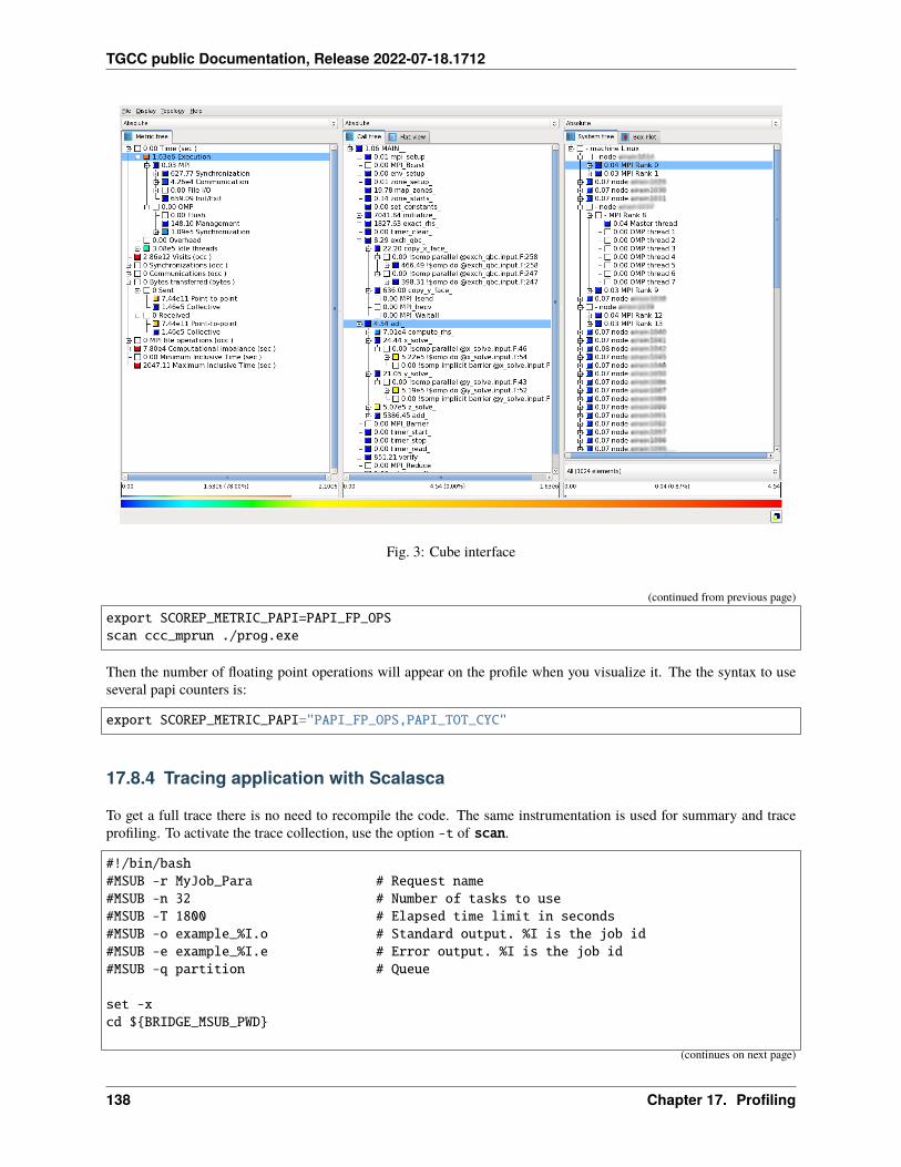
TGCC public Documentation, Release 2022-07-18.1712
Fig. 3: Cube interface
(continued from previous page)
export SCOREP_METRIC_PAPI=PAPI_FP_OPSscan ccc_mprun ./prog.exe
Then the number of floating point operations will appear on the profile when you visualize it. The the syntax to useseveral papi counters is:
export SCOREP_METRIC_PAPI="PAPI_FP_OPS,PAPI_TOT_CYC"
17.8.4 Tracing application with Scalasca
To get a full trace there is no need to recompile the code. The same instrumentation is used for summary and traceprofiling. To activate the trace collection, use the option -t of scan.
#!/bin/bash#MSUB -r MyJob_Para # Request name#MSUB -n 32 # Number of tasks to use#MSUB -T 1800 # Elapsed time limit in seconds#MSUB -o example_%I.o # Standard output. %I is the job id#MSUB -e example_%I.e # Error output. %I is the job id#MSUB -q partition # Queue
set -xcd ${BRIDGE_MSUB_PWD}
(continues on next page)
138 Chapter 17. Profiling
TGCC public Documentation, Release 2022-07-18.1712
(continued from previous page)
module load scalascaexport SCOREP_EXPERIMENT_DIRECTORY=scorep_profile.${BRIDGE_MSUB_JOBID}scan -t ccc_mprun ./prog.exe
In that case, a file traces.otf2 is created in the output directory with the summary. This profile trace can be openedwith for example.
$ tree -L 1 scorep_profile.2727202|-- profile.cubex|-- scorep.cfg|-- traces/|-- traces.def`-- traces.otf2
Warning: Generating a full trace may require a huge amount of memory.
Here is the best practice to follow:
• First start with a simple Scalasca analysis (without -t)
• Thanks to this summary, you can get an estimation of the size a full trace would take with the command:
$ square -s scorep_profile.2871901
Estimated aggregate size of event trace: 58GBEstimated requirements for largest trace buffer (max_buf): 6GB....
• If the estimated aggregated size of event trace seems excessive (it can easily reach several TB), you will need toapply filtering before recording the trace.
For more information on filtering and profiling options, check out the full documentation provided in the installationpath:
$ module load scalasca$ evince ${SCALASCA_ROOT}/share/doc/scalasca/manual/UserGuide.pdf
17.8. Scalasca 139
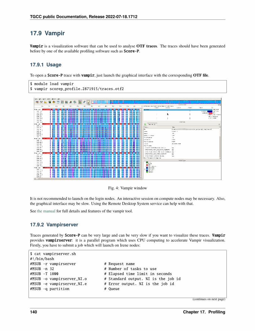
TGCC public Documentation, Release 2022-07-18.1712
17.9 Vampir
Vampir is a visualization software that can be used to analyse OTF traces. The traces should have been generatedbefore by one of the available profiling software such as Score-P.
17.9.1 Usage
To open a Score-P trace with vampir, just launch the graphical interface with the corresponding OTF file.
$ module load vampir$ vampir scorep_profile.2871915/traces.otf2
Fig. 4: Vampir window
It is not recommended to launch on the login nodes. An interactive session on compute nodes may be necessary. Also,the graphical interface may be slow. Using the Remote Desktop System service can help with that.
See the manual for full details and features of the vampir tool.
17.9.2 Vampirserver
Traces generated by Score-P can be very large and can be very slow if you want to visualize these traces. Vampirprovides vampirserver: it is a parallel program which uses CPU computing to accelerate Vampir visualization.Firstly, you have to submit a job which will launch on Irene nodes:
$ cat vampirserver.sh#!/bin/bash#MSUB -r vampirserver # Request name#MSUB -n 32 # Number of tasks to use#MSUB -T 1800 # Elapsed time limit in seconds#MSUB -o vampirserver_%I.o # Standard output. %I is the job id#MSUB -e vampirserver_%I.e # Error output. %I is the job id#MSUB -q partition # Queue
(continues on next page)
140 Chapter 17. Profiling
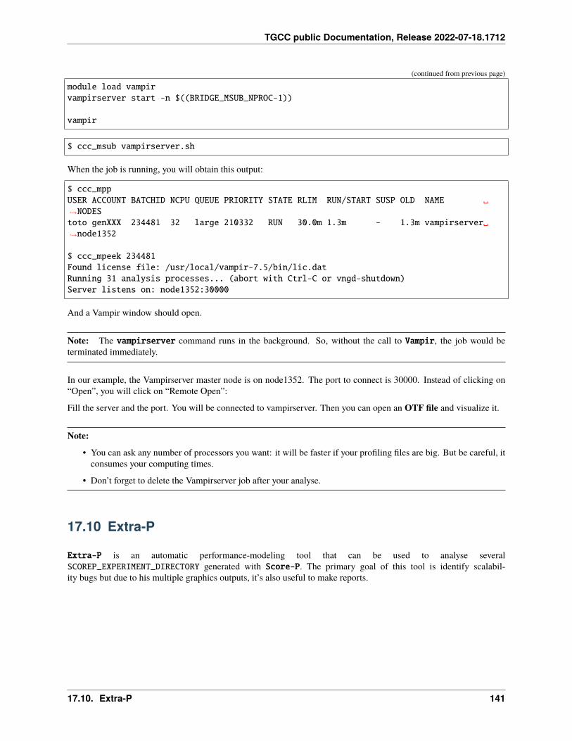
TGCC public Documentation, Release 2022-07-18.1712
(continued from previous page)
module load vampirvampirserver start -n $((BRIDGE_MSUB_NPROC-1))
vampir
$ ccc_msub vampirserver.sh
When the job is running, you will obtain this output:
$ ccc_mppUSER ACCOUNT BATCHID NCPU QUEUE PRIORITY STATE RLIM RUN/START SUSP OLD NAME ␣→˓NODEStoto genXXX 234481 32 large 210332 RUN 30.0m 1.3m - 1.3m vampirserver␣→˓node1352
$ ccc_mpeek 234481Found license file: /usr/local/vampir-7.5/bin/lic.datRunning 31 analysis processes... (abort with Ctrl-C or vngd-shutdown)Server listens on: node1352:30000
And a Vampir window should open.
Note: The vampirserver command runs in the background. So, without the call to Vampir, the job would beterminated immediately.
In our example, the Vampirserver master node is on node1352. The port to connect is 30000. Instead of clicking on“Open”, you will click on “Remote Open”:
Fill the server and the port. You will be connected to vampirserver. Then you can open an OTF file and visualize it.
Note:
• You can ask any number of processors you want: it will be faster if your profiling files are big. But be careful, itconsumes your computing times.
• Don’t forget to delete the Vampirserver job after your analyse.
17.10 Extra-P
Extra-P is an automatic performance-modeling tool that can be used to analyse severalSCOREP_EXPERIMENT_DIRECTORY generated with Score-P. The primary goal of this tool is identify scalabil-ity bugs but due to his multiple graphics outputs, it’s also useful to make reports.
17.10. Extra-P 141
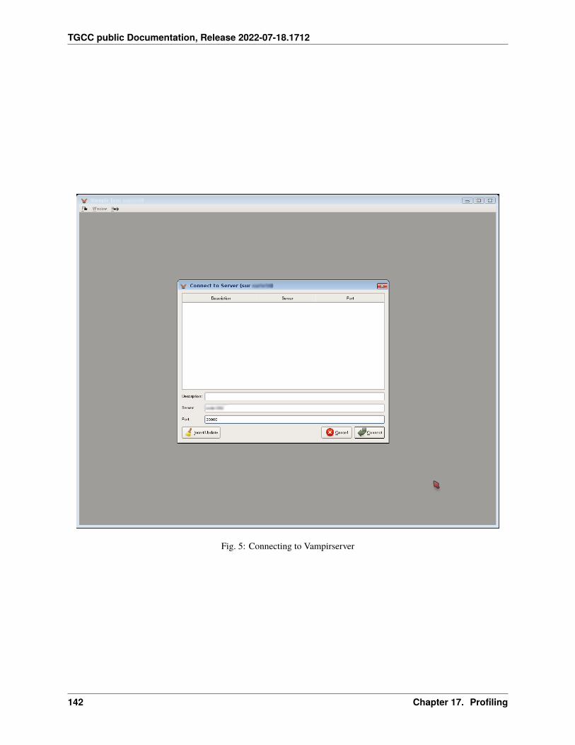
TGCC public Documentation, Release 2022-07-18.1712
Fig. 5: Connecting to Vampirserver
142 Chapter 17. Profiling
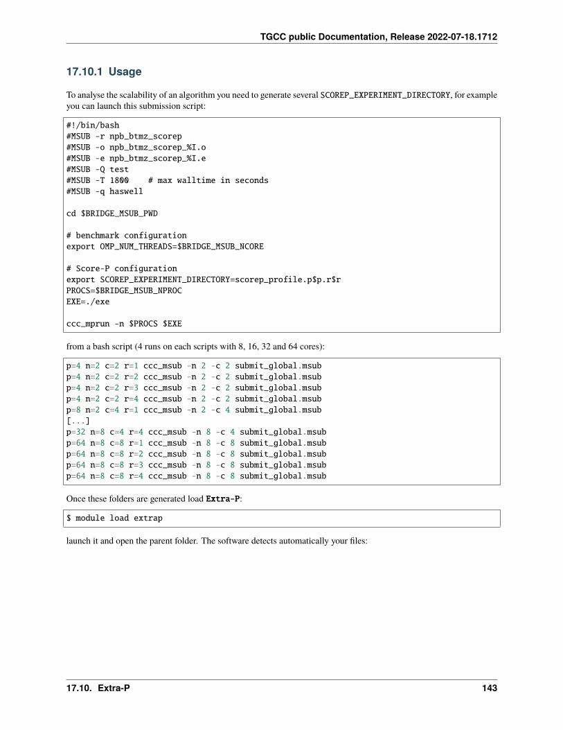
TGCC public Documentation, Release 2022-07-18.1712
17.10.1 Usage
To analyse the scalability of an algorithm you need to generate several SCOREP_EXPERIMENT_DIRECTORY, for exampleyou can launch this submission script:
#!/bin/bash#MSUB -r npb_btmz_scorep#MSUB -o npb_btmz_scorep_%I.o#MSUB -e npb_btmz_scorep_%I.e#MSUB -Q test#MSUB -T 1800 # max walltime in seconds#MSUB -q haswell
cd $BRIDGE_MSUB_PWD
# benchmark configurationexport OMP_NUM_THREADS=$BRIDGE_MSUB_NCORE
# Score-P configurationexport SCOREP_EXPERIMENT_DIRECTORY=scorep_profile.p$p.r$rPROCS=$BRIDGE_MSUB_NPROCEXE=./exe
ccc_mprun -n $PROCS $EXE
from a bash script (4 runs on each scripts with 8, 16, 32 and 64 cores):
p=4 n=2 c=2 r=1 ccc_msub -n 2 -c 2 submit_global.msubp=4 n=2 c=2 r=2 ccc_msub -n 2 -c 2 submit_global.msubp=4 n=2 c=2 r=3 ccc_msub -n 2 -c 2 submit_global.msubp=4 n=2 c=2 r=4 ccc_msub -n 2 -c 2 submit_global.msubp=8 n=2 c=4 r=1 ccc_msub -n 2 -c 4 submit_global.msub[...]p=32 n=8 c=4 r=4 ccc_msub -n 8 -c 4 submit_global.msubp=64 n=8 c=8 r=1 ccc_msub -n 8 -c 8 submit_global.msubp=64 n=8 c=8 r=2 ccc_msub -n 8 -c 8 submit_global.msubp=64 n=8 c=8 r=3 ccc_msub -n 8 -c 8 submit_global.msubp=64 n=8 c=8 r=4 ccc_msub -n 8 -c 8 submit_global.msub
Once these folders are generated load Extra-P:
$ module load extrap
launch it and open the parent folder. The software detects automatically your files:
17.10. Extra-P 143
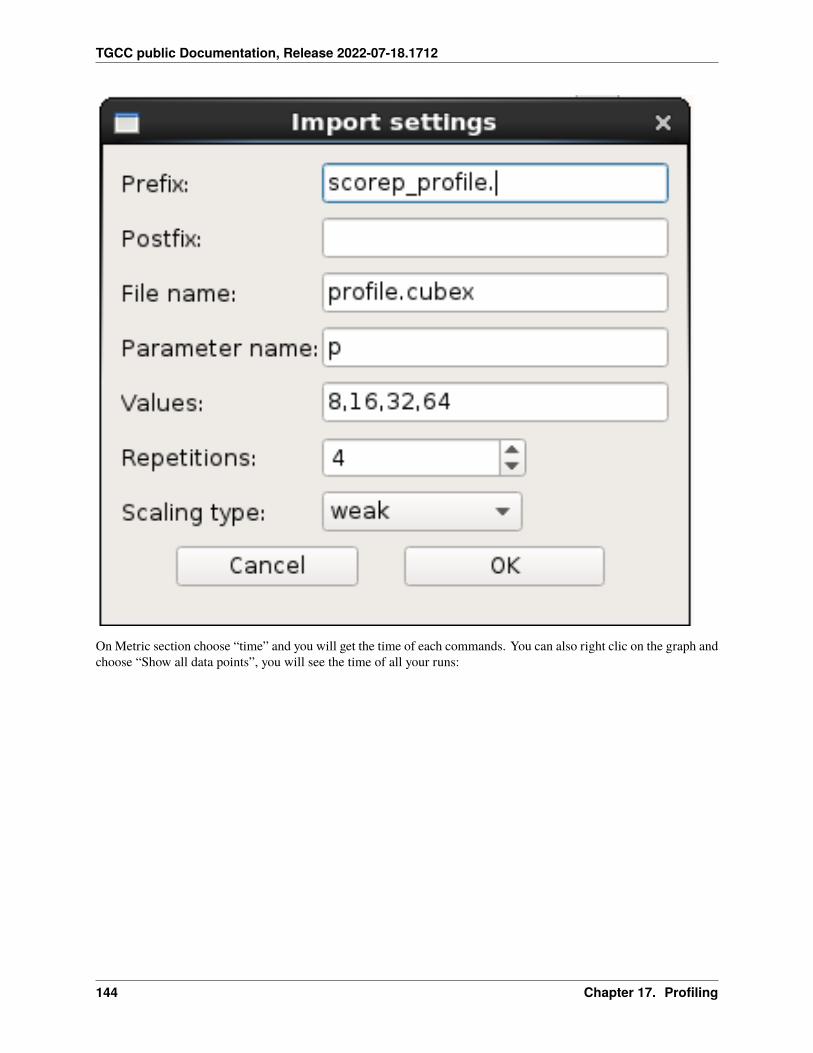
TGCC public Documentation, Release 2022-07-18.1712
On Metric section choose “time” and you will get the time of each commands. You can also right clic on the graph andchoose “Show all data points”, you will see the time of all your runs:
144 Chapter 17. Profiling
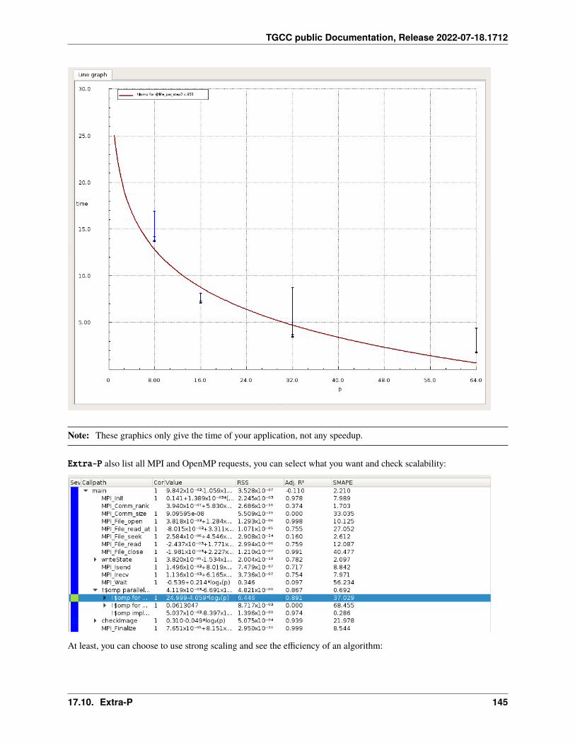
TGCC public Documentation, Release 2022-07-18.1712
Note: These graphics only give the time of your application, not any speedup.
Extra-P also list all MPI and OpenMP requests, you can select what you want and check scalability:
At least, you can choose to use strong scaling and see the efficiency of an algorithm:
17.10. Extra-P 145
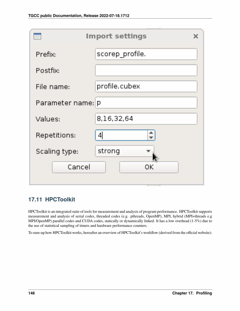
TGCC public Documentation, Release 2022-07-18.1712
17.11 HPCToolkit
HPCToolkit is an integrated suite of tools for measurement and analysis of program performance. HPCToolkit supportsmeasurement and analysis of serial codes, threaded codes (e.g. pthreads, OpenMP), MPI, hybrid (MPI+threads e.gMPI/OpenMP) parallel codes and CUDA codes, statically or dynamically linked. It has a low overhead (1-5%) due tothe use of statistical sampling of timers and hardware performance counters.
To sum-up how HPCToolkit works, hereafter an overview of HPCToolkit’s workflow (derived from the official website):
146 Chapter 17. Profiling
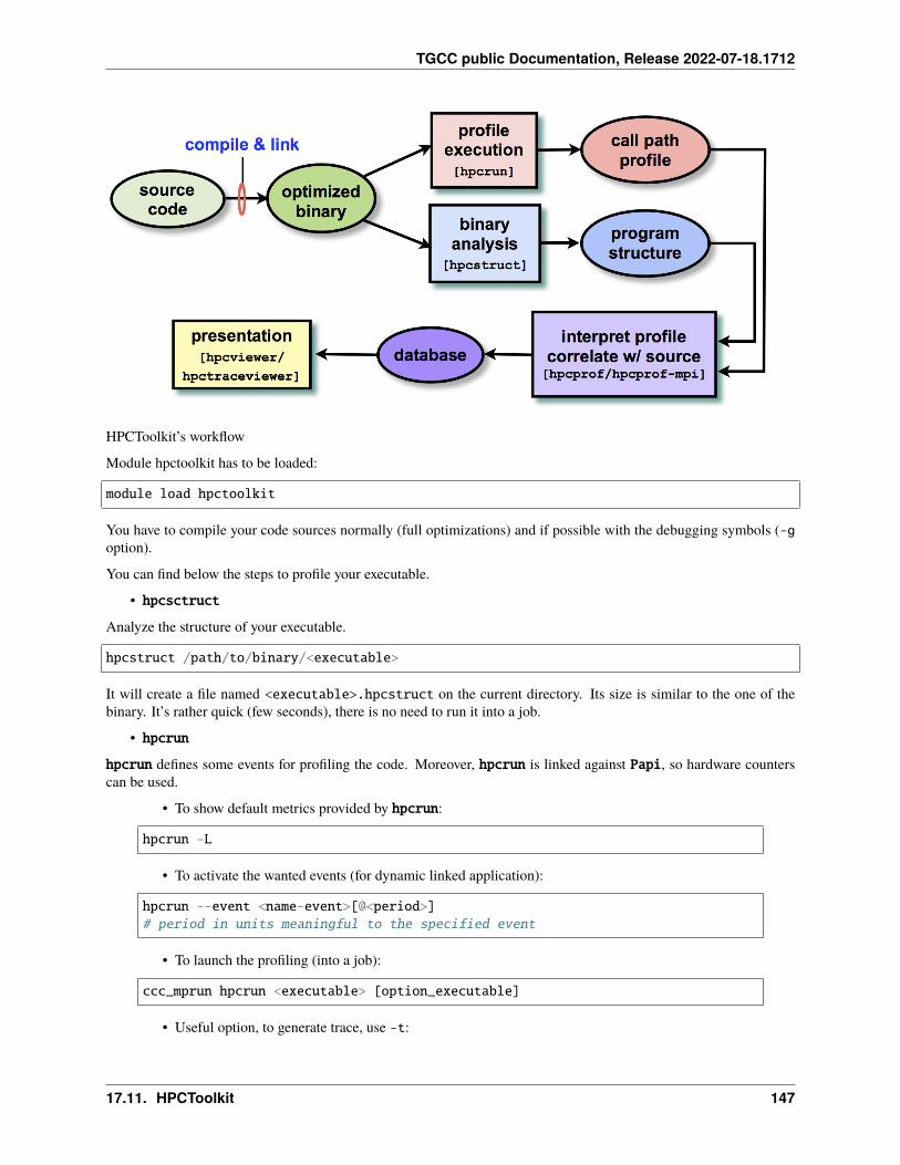
TGCC public Documentation, Release 2022-07-18.1712
HPCToolkit’s workflow
Module hpctoolkit has to be loaded:
module load hpctoolkit
You have to compile your code sources normally (full optimizations) and if possible with the debugging symbols (-goption).
You can find below the steps to profile your executable.
• hpcsctruct
Analyze the structure of your executable.
hpcstruct /path/to/binary/<executable>
It will create a file named <executable>.hpcstruct on the current directory. Its size is similar to the one of thebinary. It’s rather quick (few seconds), there is no need to run it into a job.
• hpcrun
hpcrun defines some events for profiling the code. Moreover, hpcrun is linked against Papi, so hardware counterscan be used.
• To show default metrics provided by hpcrun:
hpcrun -L
• To activate the wanted events (for dynamic linked application):
hpcrun --event <name-event>[@<period>]# period in units meaningful to the specified event
• To launch the profiling (into a job):
ccc_mprun hpcrun <executable> [option_executable]
• Useful option, to generate trace, use -t:
17.11. HPCToolkit 147
TGCC public Documentation, Release 2022-07-18.1712
hpcrun -t ...
A directory named hpctoolkit-<executable>-measurement-<jod_id> will be created.
• hpcrun-flat
Another way to profile an executable is to use hpcrun-flat, which profiles the execution using statistical sampling(rather than instrumentation) and generates flat profile files. Only dynamic linked applications can be profiled, due tousing preloaded shared libraries to initiate profiling.
• To show default metrics provided by hpcrun-flat:
hpcrun-flat -lhpcrun-flat -L #more verbose
• To activate the wanted events (for dynamic linked applications):
hpcrun-flat --event <event-name>[:<period>]#period in units meaningful to the specified event
• To launch the profiling (into a job):
ccc_mprun hpcrun-flat [options][events] [--] <executable> [option_executable]
If there are at least one option following your executable has, put the option -- to hpcrun-flat.
Many files named <executable>.hpcrun-flat.<hostname>.<pid>.<flavor> will be created. Some options ofare available to sort them.
Note: Only POSIX threads are supported.
Note: The WALLCLOCK event cannot be used in a multithreaded process.
• hpcprof / hpcprof-mpi
hpcprof analyses call path profile performance measurements according to the source code structure and generates anexperiment database for use with hpcviewer. The mpi-version accelerates correlation time.
$ hpcprof -S <executable>.hpcstruct -I /path/to/source/1/'*' -I /path/to/source/2/+ hpctoolkit-<executable>-measurement-<job_id>
$ ccc_mprun hpcprof-mpi -S <executable>.hpcstruct -I /path/to/source/1/* -I/path/to/source/2/+ hpctoolkit-<executable>-measurement-<job_id>
• * search for file in the specified directory only
• + search for file recursively
A directory named hpctoolkit-<executable>-database-<number>-[<number>-...] will be created.
• hpcproftt
hpcproftt correlates ‘flat’ profile metrics provided by hpcrun-flat with either source code structure or object codeand generates textual output.
148 Chapter 17. Profiling
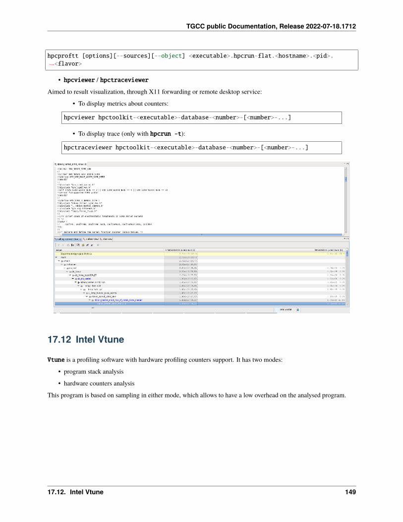
TGCC public Documentation, Release 2022-07-18.1712
hpcproftt [options][--sources][--object] <executable>.hpcrun-flat.<hostname>.<pid>.→˓<flavor>
• hpcviewer / hpctraceviewer
Aimed to result visualization, through X11 forwarding or remote desktop service:
• To display metrics about counters:
hpcviewer hpctoolkit-<executable>-database-<number>-[<number>-...]
• To display trace (only with hpcrun -t):
hpctraceviewer hpctoolkit-<executable>-database-<number>-[<number>-...]
17.12 Intel Vtune
Vtune is a profiling software with hardware profiling counters support. It has two modes:
• program stack analysis
• hardware counters analysis
This program is based on sampling in either mode, which allows to have a low overhead on the analysed program.
17.12. Intel Vtune 149
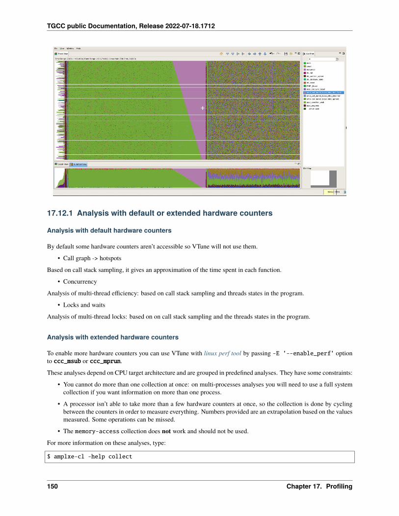
TGCC public Documentation, Release 2022-07-18.1712
17.12.1 Analysis with default or extended hardware counters
Analysis with default hardware counters
By default some hardware counters aren’t accessible so VTune will not use them.
• Call graph -> hotspots
Based on call stack sampling, it gives an approximation of the time spent in each function.
• Concurrency
Analysis of multi-thread efficiency: based on call stack sampling and threads states in the program.
• Locks and waits
Analysis of multi-thread locks: based on on call stack sampling and the threads states in the program.
Analysis with extended hardware counters
To enable more hardware counters you can use VTune with linux perf tool by passing -E '--enable_perf' optionto ccc_msub or ccc_mprun.
These analyses depend on CPU target architecture and are grouped in predefined analyses. They have some constraints:
• You cannot do more than one collection at once: on multi-processes analyses you will need to use a full systemcollection if you want information on more than one process.
• A processor isn’t able to take more than a few hardware counters at once, so the collection is done by cyclingbetween the counters in order to measure everything. Numbers provided are an extrapolation based on the valuesmeasured. Some operations can be missed.
• The memory-access collection does not work and should not be used.
For more information on these analyses, type:
$ amplxe-cl -help collect
150 Chapter 17. Profiling
TGCC public Documentation, Release 2022-07-18.1712
The lightweight hotspots analysis is a special case of hotspots analysis which use the collecting driver. It has a loweroverhead than the hotspots analysis but has the same constraints than the hardware counters mode.
Never do a collection on a non exclusive reservation of the node (the results may strongly be influenced by potentialother running jobs).
The best practice is to do a collection in batch mode and then open the result file in the GUI. The visualisation GUIcan use a lot of resource, so it is best to avoid using it directly on the login nodes.
17.12.2 Collection in batch mode
• hotspots_vtune.msub
#!/bin/bash#MSUB -n 1#MSUB -c 28#MSUB -T 1800#MSUB -q {Partition}#MSUB -x### Do a hotspots collection on a node using a test case on 28 OMP threads##
module load vtune
export OMP_NUM_THREADS=${BRIDGE_MSUB_NCORE}
ccc_mprun -E '--enable_perf' amplxe-cl -collect hotspots -r ${PWD}/vtune_results ./test
Always set the analysis_type and be sure to use a collection type compatible with the processors of the partition youare running on. Also, make sure your working directory is either on SCRATCH or WORK filesystem so no files willbe generated on your home filesystem (NFS) as it would show slow performance.
17.12.3 Open Visualization GUI
On a remote X display do:
• interactive_vtune.msub
#!/bin/bash#MSUB -n 1#MSUB -T 1800#MSUB -q {Partition}#MSUB -X#MSUB -x### launch the vtune GUI on a standard node for visualisation of a collection##module load vtuneccc_mprun amplxe-gui
To speed up performance, you can move your profiling files into /tmp or /dev/shm folder before opening them withvtune.
Once the GUI appears you can visualize results from the analyses.
17.12. Intel Vtune 151
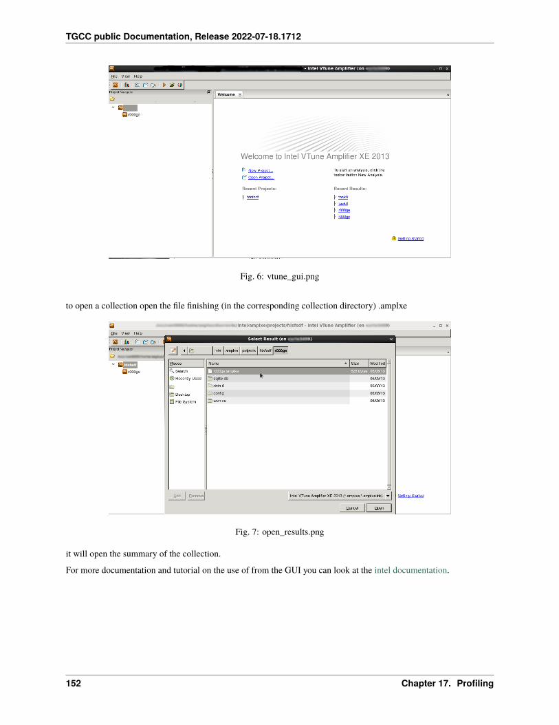
TGCC public Documentation, Release 2022-07-18.1712
Fig. 6: vtune_gui.png
to open a collection open the file finishing (in the corresponding collection directory) .amplxe
Fig. 7: open_results.png
it will open the summary of the collection.
For more documentation and tutorial on the use of from the GUI you can look at the intel documentation.
152 Chapter 17. Profiling
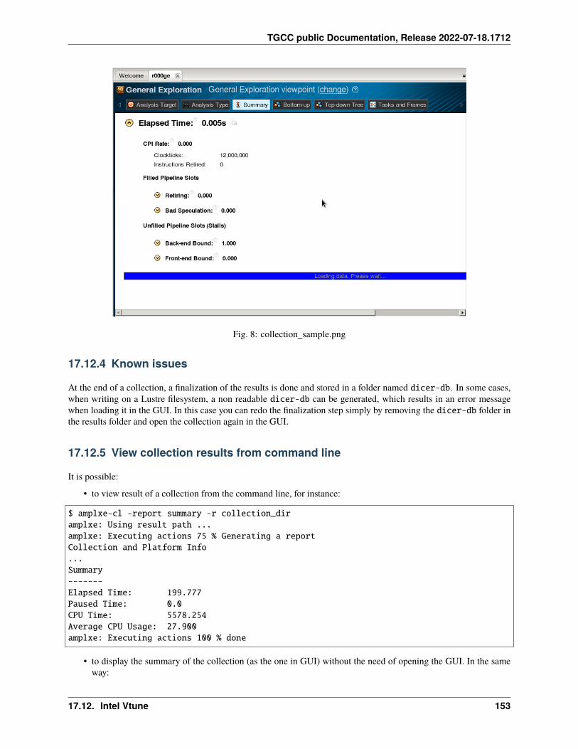
TGCC public Documentation, Release 2022-07-18.1712
Fig. 8: collection_sample.png
17.12.4 Known issues
At the end of a collection, a finalization of the results is done and stored in a folder named dicer-db. In some cases,when writing on a Lustre filesystem, a non readable dicer-db can be generated, which results in an error messagewhen loading it in the GUI. In this case you can redo the finalization step simply by removing the dicer-db folder inthe results folder and open the collection again in the GUI.
17.12.5 View collection results from command line
It is possible:
• to view result of a collection from the command line, for instance:
$ amplxe-cl -report summary -r collection_diramplxe: Using result path ...amplxe: Executing actions 75 % Generating a reportCollection and Platform Info...Summary-------Elapsed Time: 199.777Paused Time: 0.0CPU Time: 5578.254Average CPU Usage: 27.900amplxe: Executing actions 100 % done
• to display the summary of the collection (as the one in GUI) without the need of opening the GUI. In the sameway:
17.12. Intel Vtune 153
TGCC public Documentation, Release 2022-07-18.1712
$ amplxe-cl -report hotspots -r collection_diramplxe: Using result path ...amplxe: Executing actions 75 % Generating a reportFunction CPU Time ...main$omp$parallel@18 4872.548s ......amplxe: Executing actions 100 % done
• to list the hotspots in a top down display.
For a detailed help on this, see:
$ amplxe-cl -help report
17.12.6 Generate a dot graph with gprof2dot
To generate a graph with gprof2dot, see gprof2dot and VTune.
17.13 Valgrind
Valgrind is an instrumentation framework for dynamic analysis tools. It comes with a set of tools for profiling anddebugging codes.
To run a program with valgrind, there is no need to instrument, recompile, or otherwise modify the code.
Note: A tool in the Valgrind distribution can be invoked with the --tool option:
module load valgrindvalgrind --tool=<toolname> #default is memcheck
17.13.1 Callgrind
Callgrind is a profiling tool that records the call history among functions in a program’s run as a call-graph. By default,the collected data consists of the number of instructions executed, their relationship to source lines, the caller/calleerelationship between functions, and the numbers of such calls.
To start a profile run for a program, execute:
module load valgrindvalgrind --tool=callgrind [callgrind options] your-program [program options]
While the simulation is running, you can observe the execution with:
callgrind_control -b
This will print out the current backtrace. To annotate the backtrace with event counts, run:
callgrind_control -e -b
154 Chapter 17. Profiling
TGCC public Documentation, Release 2022-07-18.1712
After program termination, a profile data file named callgrind.out.<pid> is generated, where pid is the processID of the program being profiled. The data file contains information about the calls made in the program among thefunctions executed, together with Instruction Read (Ir) event counts.
To generate a function-by-function summary from the profile data file, use:
callgrind_annotate [options] callgrind.out.<pid>
17.13.2 Cachegrind
Cachegrind simulates how your program interacts with a machine’s cache hierarchy and (optionally) branch predictor.To run cachegrind on a program prog, you must specify --tool=cachegrind on the valgrind command line:
module load valgrindvalgrind --tool=cachegrind prog
Branch prediction statistics are not collected by default. To do so, add the option --branch-sim=yes.
valgrind -tool=cachegrind --branch-sim=yes prog
One output file will be created for each process launched with cachegrind. To analyse the output, use the commandcg_annotate:
$ cg_annotate <output_file>
cg_annotate can show the source codes annotated with the sampled values. Therefore, either use the option--auto=yes to apply to all the available source files or specify one file by passing it as an argument.
$ cg_annotate <output_file> sourcecode.c
For more information on Cachegrind, check out the official Cachegrind User Manual.
17.13.3 Massif
Massif measures how much heap memory a program uses. This includes both the useful space, and the extra bytesallocated for book-keeping and alignment purposes. Massif can optionally measure the stack memory.
As for the other Valgrind tools, the program should be compiled with debugging info (the -g option). To run massifon a program prog, the valgrind command line is:
module load valgrindvalgrind --tool=massif prog
The Massif option --pages-as-heap=yes allows to measure all the memory used by the program.
By default, the output file is called massif.out.<pid> (pid is the process ID), although this file name can be changedwith the --massif-out-file option. To present the heap profiling information about the program in a readable way,run ms_print:
$ ms_print massif.out.<pid>
17.13. Valgrind 155
TGCC public Documentation, Release 2022-07-18.1712
17.14 Intel Advisor
Intel Advisor is a threading design and prototyping tool for software architects. Intel Advisor is a useful tool for:
• analysing, designing, tuning and checking your threading design before implementation,
• exploring and testing threading options without disrupting normal development,
• predicting thread errors & performance scaling on systems with more cores.
Intel Advisor is available through the module command:
$ module load advisor
The tool can be called either via the command line interface (command advixe-cl) or the GUI (commandadvixe-gui). Launching the code needs to be done in a submission script or an interactive session. Never on thelogin nodes.
17.14.1 Intel Advisor Command Line Interface
The Intel Advisor command line interface helps you to:
• collect results in three possible modes: survey, suitability, and correctness,
• perform regression testing to determine if source code changes introduced new problems,
• generate predefined reports in several formats.
The advixe-cl invokes the Intel Advisor command line interface:
$ module load advisor$ advixe-cl <-action> [-option] [[--] application [application options]]
One action is to be specified per command line, such as: -collect, -collect-list, -report, -report-list,-format-list, -help, -import-dir, or -version. Some actions require arguments, such as -collect and-report.
Results cannot be viewed on the command line. You can use the Intel Advisor GUI, preferably in an interactive sessionwith X11 forwarding or with a Remote Desktop session, to view a result, or use command line tools to generate one ormore reports from the result.
To display the built-in documentation, please type:
$ advixe-cl -help
17.14.2 Intel Advisor GUI
Submission script example:
#MSUB -r advisor_sub#MSUB -q partition#MSUB -n 1 # Number of task#MSUB -c 28 # Number of core per task#MSUB -o advisor_sub_%J.e # Error output#MSUB -e advisor_sub_%J.o # Output#MSUB -x
(continues on next page)
156 Chapter 17. Profiling
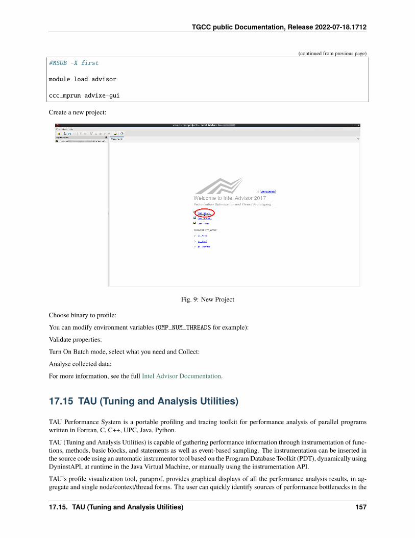
TGCC public Documentation, Release 2022-07-18.1712
(continued from previous page)
#MSUB -X first
module load advisor
ccc_mprun advixe-gui
Create a new project:
Fig. 9: New Project
Choose binary to profile:
You can modify environment variables (OMP_NUM_THREADS for example):
Validate properties:
Turn On Batch mode, select what you need and Collect:
Analyse collected data:
For more information, see the full Intel Advisor Documentation.
17.15 TAU (Tuning and Analysis Utilities)
TAU Performance System is a portable profiling and tracing toolkit for performance analysis of parallel programswritten in Fortran, C, C++, UPC, Java, Python.
TAU (Tuning and Analysis Utilities) is capable of gathering performance information through instrumentation of func-tions, methods, basic blocks, and statements as well as event-based sampling. The instrumentation can be inserted inthe source code using an automatic instrumentor tool based on the Program Database Toolkit (PDT), dynamically usingDyninstAPI, at runtime in the Java Virtual Machine, or manually using the instrumentation API.
TAU’s profile visualization tool, paraprof, provides graphical displays of all the performance analysis results, in ag-gregate and single node/context/thread forms. The user can quickly identify sources of performance bottlenecks in the
17.15. TAU (Tuning and Analysis Utilities) 157
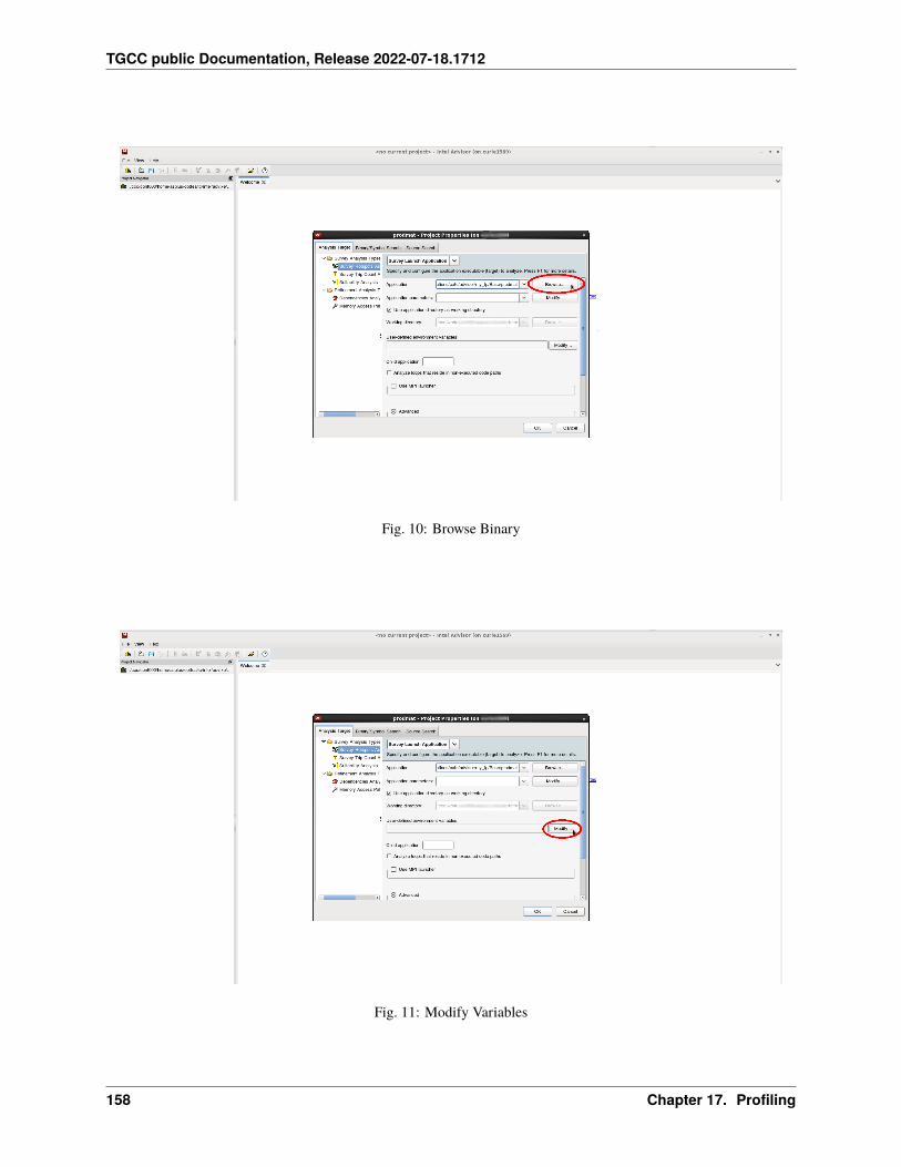
TGCC public Documentation, Release 2022-07-18.1712
Fig. 10: Browse Binary
Fig. 11: Modify Variables
158 Chapter 17. Profiling
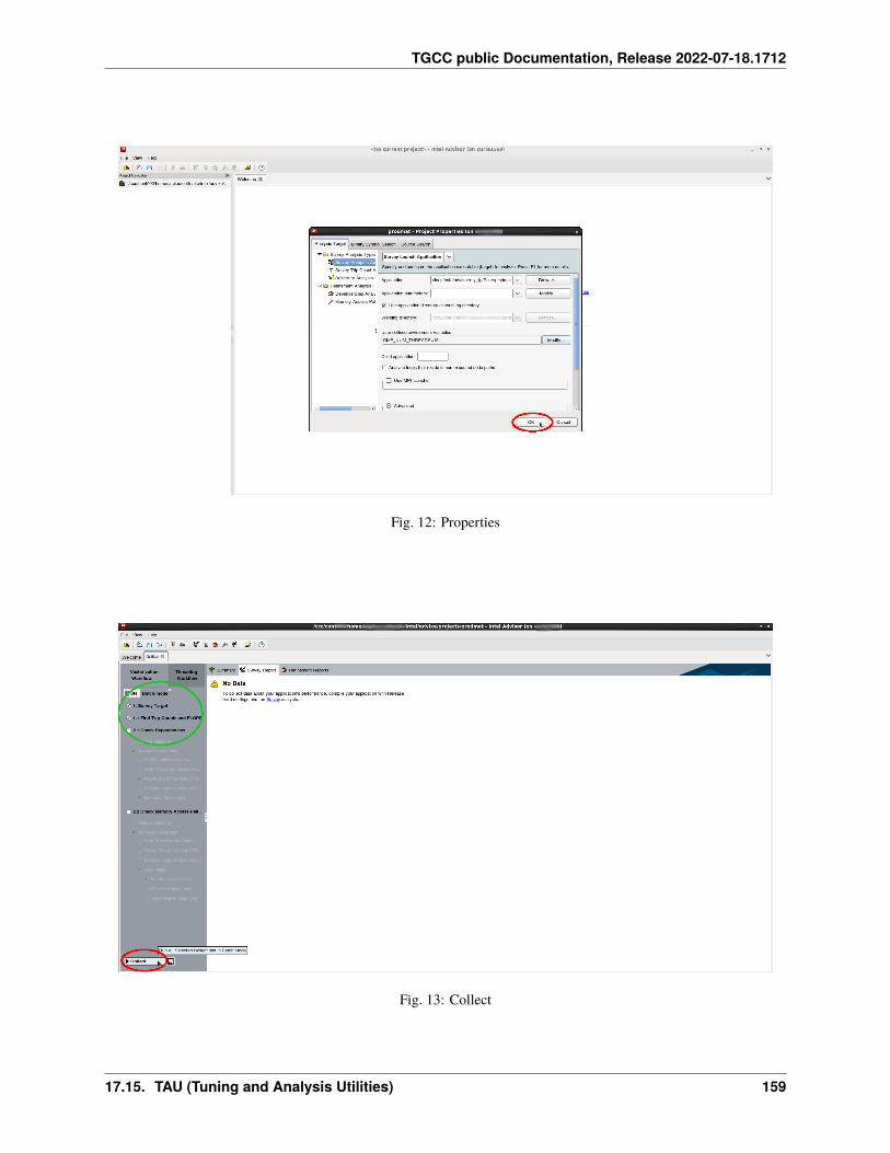
TGCC public Documentation, Release 2022-07-18.1712
Fig. 12: Properties
Fig. 13: Collect
17.15. TAU (Tuning and Analysis Utilities) 159
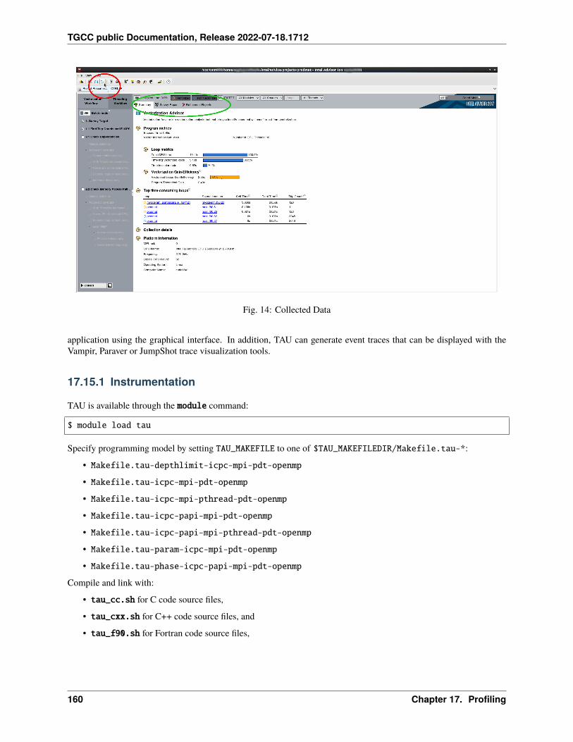
TGCC public Documentation, Release 2022-07-18.1712
Fig. 14: Collected Data
application using the graphical interface. In addition, TAU can generate event traces that can be displayed with theVampir, Paraver or JumpShot trace visualization tools.
17.15.1 Instrumentation
TAU is available through the module command:
$ module load tau
Specify programming model by setting TAU_MAKEFILE to one of $TAU_MAKEFILEDIR/Makefile.tau-*:
• Makefile.tau-depthlimit-icpc-mpi-pdt-openmp
• Makefile.tau-icpc-mpi-pdt-openmp
• Makefile.tau-icpc-mpi-pthread-pdt-openmp
• Makefile.tau-icpc-papi-mpi-pdt-openmp
• Makefile.tau-icpc-papi-mpi-pthread-pdt-openmp
• Makefile.tau-param-icpc-mpi-pdt-openmp
• Makefile.tau-phase-icpc-papi-mpi-pdt-openmp
Compile and link with:
• tau_cc.sh for C code source files,
• tau_cxx.sh for C++ code source files, and
• tau_f90.sh for Fortran code source files,
160 Chapter 17. Profiling
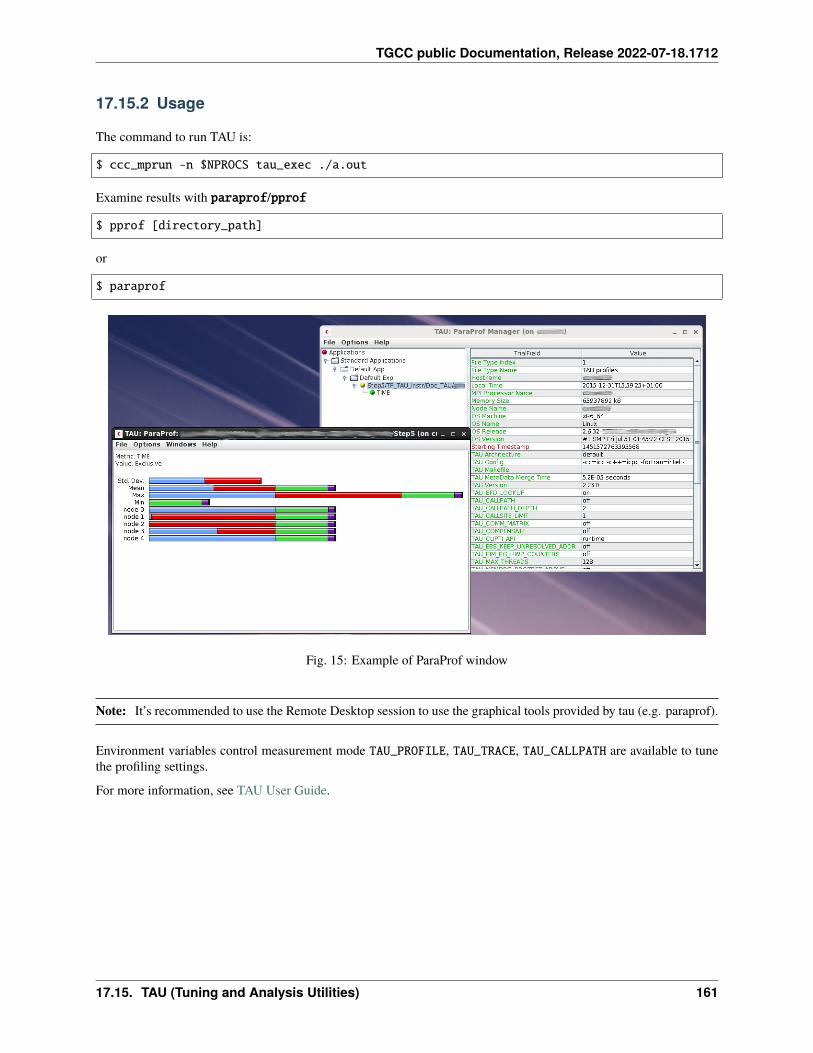
TGCC public Documentation, Release 2022-07-18.1712
17.15.2 Usage
The command to run TAU is:
$ ccc_mprun -n $NPROCS tau_exec ./a.out
Examine results with paraprof/pprof
$ pprof [directory_path]
or
$ paraprof
Fig. 15: Example of ParaProf window
Note: It’s recommended to use the Remote Desktop session to use the graphical tools provided by tau (e.g. paraprof).
Environment variables control measurement mode TAU_PROFILE, TAU_TRACE, TAU_CALLPATH are available to tunethe profiling settings.
For more information, see TAU User Guide.
17.15. TAU (Tuning and Analysis Utilities) 161
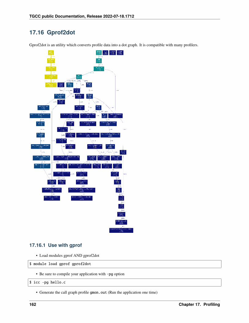
TGCC public Documentation, Release 2022-07-18.1712
17.16 Gprof2dot
Gprof2dot is an utility which converts profile data into a dot graph. It is compatible with many profilers.
17.16.1 Use with gprof
• Load modules gprof AND gprof2dot
$ module load gprof gprof2dot
• Be sure to compile your application with -pg option
$ icc -pg hello.c
• Generate the call graph profile gmon.out (Run the application one time)
162 Chapter 17. Profiling
TGCC public Documentation, Release 2022-07-18.1712
$ ./a.out
• Generate the dot graph in a PNG image
$ gprof ./a.out gmon.out | gprof2dot.py | dot -Tpng -o a.png
17.16.2 Use with VTune in command line
• Load modules VTune AND gprof2dot
$ module load vtune gprof2dot
• Use VTune to collect data
$ ccc_mprun amplxe-cl -collect hotspots -result-dir output -- ./exe
• Transform data in a gprof-like file
$ amplxe-cl -report gprof-cc -result-dir output -format text -report-output output.txt
• Generate the dot graph
$ gprof2dot.py -f axe output.txt | dot -Tpng -o output.png
For more information about gprof2dot, see GitHub gprof2dot.
17.17 Perf
Perf is a portable tool included in Linux kernel, it doesn’t need to be loaded, doesn’t need any driver and also works onall Linux platforms.
It is a performance analysis tool which displays performance counters such as the number of cache loads misses orbranch loads misses.
• Perf cannot be fully launched on login nodes, you will need to execute it on compute node(s).
• To run a command and gather performance counter statistics use perf stat. Here is a simple job example:
#!/bin/bash#MSUB -n 1#MSUB -c 12#MSUB -T 400#MSUB -q |Partition|#MSUB -x#MSUB -E '--enable_perf'
export OMP_NUM_THREADS=${BRIDGE_MSUB_NCORE}
ccc_mprun perf stat -o perf.log ./exe
• Informations will be stored in perf.log:
17.17. Perf 163
TGCC public Documentation, Release 2022-07-18.1712
$ cat perf.log# started on Wed Oct 11 14:01:14 2017
Performance counter stats for './exe':
50342.076495 task-clock:u (msec) # 1.000 CPUs utilized98,323 page-faults:u # 0.002 M/sec155,516,791,925 cycles:u # 3.089 GHz197,715,764,466 instructions:u # 1.27 insn per cycle
50.348439743 seconds time elapsed
Now for more specifics counters:
• list of all performance counters with the command perf list
• Use the -e option to specify the wanted performance counters. For example, to get how much cache accessmisses within all cache access:
$ ccc_mprun perf stat -o perf.log -e cache-references,cache-misses ./exe$ cat perf.log# started on Wed Oct 11 14:02:52 2017
Performance counter stats for './exe':
8,654,163,728 cache-references:u875,346,349 cache-misses:u # 10.115 % of all cache refs
52.710267128 seconds time elapsed
Perf can also record few counters from an executable and create a report:
• Use a job to create a report with
$ ccc_mprun -vvv perf record -o data.perf ./exe...[ perf record: Woken up 53 times to write data ][ perf record: Captured and wrote 13.149 MB data.perf (344150 samples) ]...
• Read the report from the login node
$ perf report -i data.perfSamples: 344K of event 'cycles:u', Event count (approx.): 245940413046Overhead Command Shared Object Symbol99.94% exe exe [.] mydgemm_0.02% exe [kernel.vmlinux] [k] apic_timer_interrupt0.02% exe [kernel.vmlinux] [k] page_fault0.00% exe exe [.] MAIN__...
• You can also using call graphs with
$ ccc_mprun -vvv perf record --call-graph fp -o data.perf ./exe
(continues on next page)
164 Chapter 17. Profiling
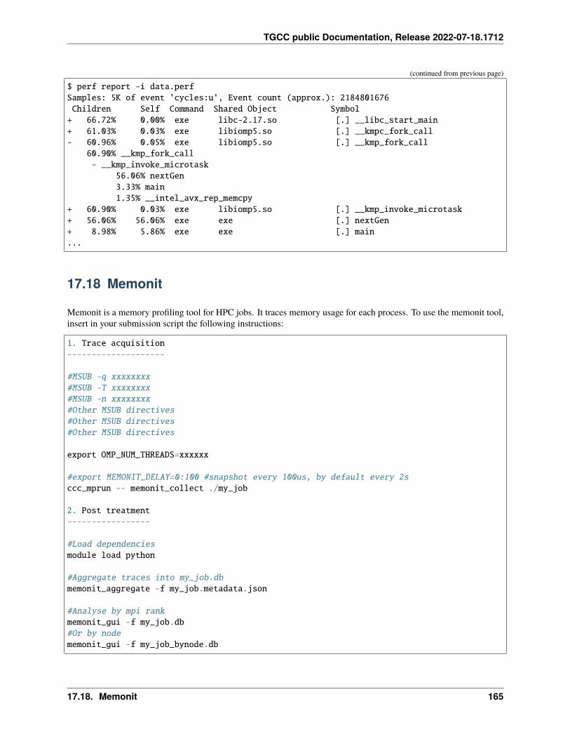
TGCC public Documentation, Release 2022-07-18.1712
(continued from previous page)
$ perf report -i data.perfSamples: 5K of event 'cycles:u', Event count (approx.): 2184801676Children Self Command Shared Object Symbol+ 66.72% 0.00% exe libc-2.17.so [.] __libc_start_main+ 61.03% 0.03% exe libiomp5.so [.] __kmpc_fork_call- 60.96% 0.05% exe libiomp5.so [.] __kmp_fork_call
60.90% __kmp_fork_call- __kmp_invoke_microtask
56.06% nextGen3.33% main1.35% __intel_avx_rep_memcpy
+ 60.90% 0.03% exe libiomp5.so [.] __kmp_invoke_microtask+ 56.06% 56.06% exe exe [.] nextGen+ 8.98% 5.86% exe exe [.] main...
17.18 Memonit
Memonit is a memory profiling tool for HPC jobs. It traces memory usage for each process. To use the memonit tool,insert in your submission script the following instructions:
1. Trace acquisition--------------------
#MSUB -q xxxxxxxx#MSUB -T xxxxxxxx#MSUB -n xxxxxxxx#Other MSUB directives#Other MSUB directives#Other MSUB directives
export OMP_NUM_THREADS=xxxxxx
#export MEMONIT_DELAY=0:100 #snapshot every 100us, by default every 2sccc_mprun -- memonit_collect ./my_job
2. Post treatment-----------------
#Load dependenciesmodule load python
#Aggregate traces into my_job.dbmemonit_aggregate -f my_job.metadata.json
#Analyse by mpi rankmemonit_gui -f my_job.db#Or by nodememonit_gui -f my_job_bynode.db
17.18. Memonit 165
TGCC public Documentation, Release 2022-07-18.1712
166 Chapter 17. Profiling

CHAPTER
EIGHTEEN
POST-PROCESSING
18.1 Gnuplot
The Gnuplot homepage provides links to all the documentation most users will need.
You can use gnuplot from a Remote Desktop System session or from a compute node (please avoid login nodes)
To start gnuplot from a Remote Desktop System session:
• Start your Remote Desktop System session
• Open a terminal
module load gnuplotgnuplot
To start gnuplot from a compute node:
• Log into the login node, with X redirection (ssh -X login@login-node).
• Load the appropriate module:
module load gnuplot
• Start an interactive session from a compute node with X11 export and launch gnuplot:
ccc_mprun -Xfirst -T3600 -p <partition> -sgnuplot
• An example of gnuplot prompt:
$ gnuplot
G N U P L O TVersion x.y patchlevel z last modified 2020-12-01
Copyright (C) 1986-1993, 1998, 2004, 2007-2020Thomas Williams, Colin Kelley and many others
gnuplot home: http://www.gnuplot.infofaq, bugs, etc: type "help FAQ"immediate help: type "help" (plot window: hit 'h')
Terminal type is now 'unknown'gnuplot>
167
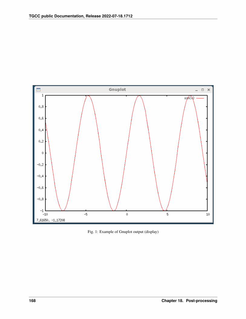
TGCC public Documentation, Release 2022-07-18.1712
Fig. 1: Example of Gnuplot output (display)
168 Chapter 18. Post-processing
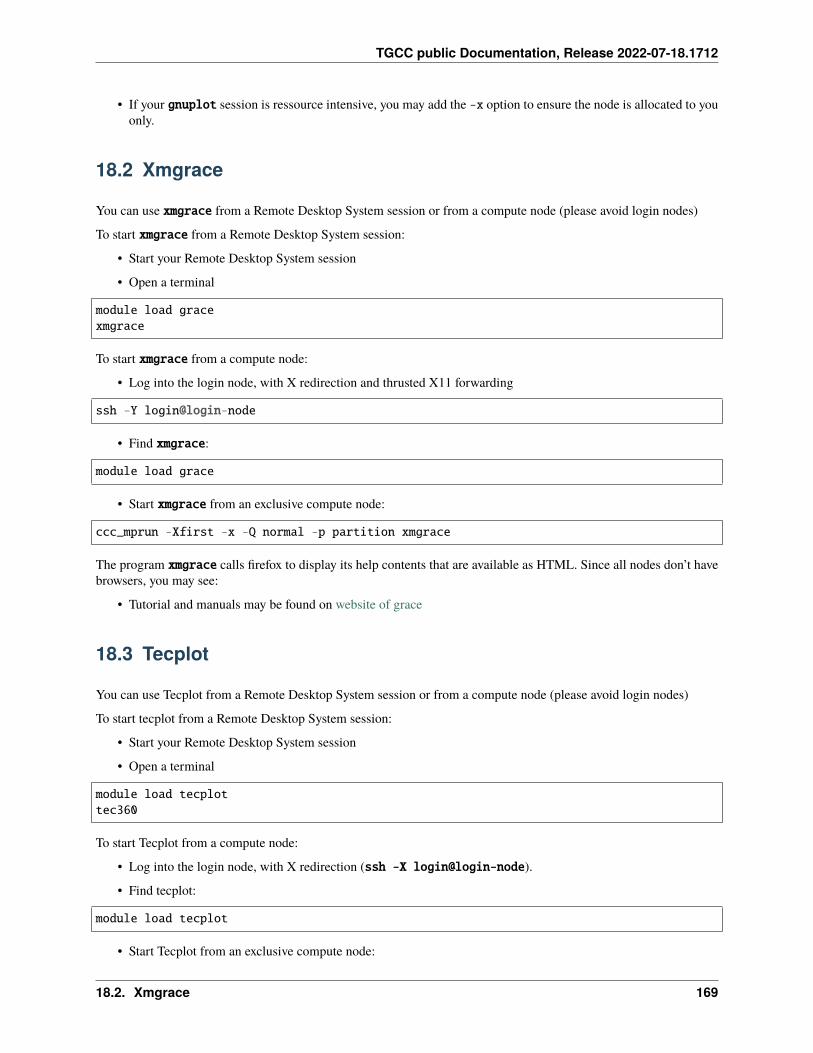
TGCC public Documentation, Release 2022-07-18.1712
• If your gnuplot session is ressource intensive, you may add the -x option to ensure the node is allocated to youonly.
18.2 Xmgrace
You can use xmgrace from a Remote Desktop System session or from a compute node (please avoid login nodes)
To start xmgrace from a Remote Desktop System session:
• Start your Remote Desktop System session
• Open a terminal
module load gracexmgrace
To start xmgrace from a compute node:
• Log into the login node, with X redirection and thrusted X11 forwarding
ssh -Y login@login-node
• Find xmgrace:
module load grace
• Start xmgrace from an exclusive compute node:
ccc_mprun -Xfirst -x -Q normal -p partition xmgrace
The program xmgrace calls firefox to display its help contents that are available as HTML. Since all nodes don’t havebrowsers, you may see:
• Tutorial and manuals may be found on website of grace
18.3 Tecplot
You can use Tecplot from a Remote Desktop System session or from a compute node (please avoid login nodes)
To start tecplot from a Remote Desktop System session:
• Start your Remote Desktop System session
• Open a terminal
module load tecplottec360
To start Tecplot from a compute node:
• Log into the login node, with X redirection (ssh -X login@login-node).
• Find tecplot:
module load tecplot
• Start Tecplot from an exclusive compute node:
18.2. Xmgrace 169
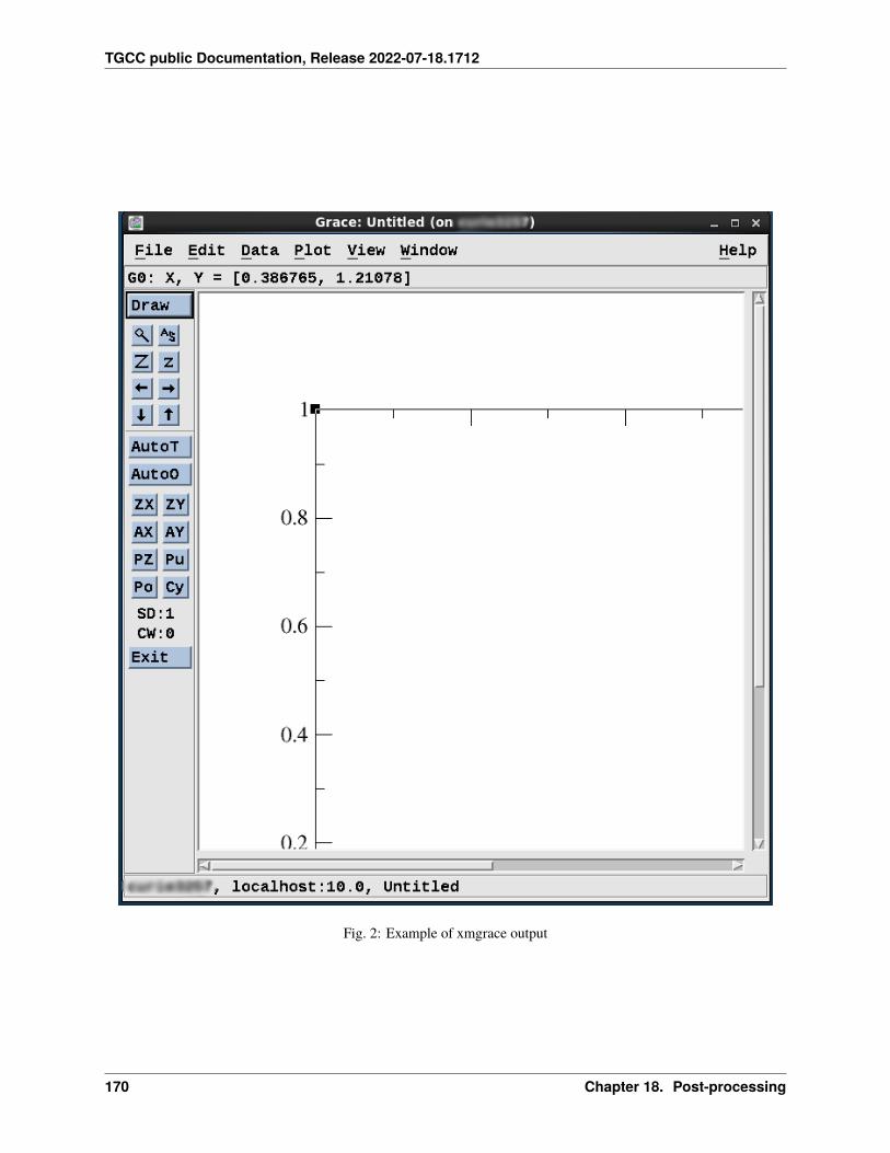
TGCC public Documentation, Release 2022-07-18.1712
Fig. 2: Example of xmgrace output
170 Chapter 18. Post-processing
TGCC public Documentation, Release 2022-07-18.1712
ccc_mprun -Xfirst -x -Q normal -p partition tec360
Tecplot calls firefox to display its help contents that are available as HTML. Since not all node have firefox, you maybe interested in the following:
• tutorial
• forum
18.4 Ensight
The tool can be launched from a Remote Desktop System session (highly recommended) or from a compute node.Please avoid login nodes!
From a Remote Desktop System session:
• Start your Remote Desktop System session
• Open a terminal
module load ensightensight101
From a compute node:
• Connect to the supercomputer with trusted X11 forwarding
ssh -XY <login>@<machine>
• Load ensight
module load ensight
• Start the tool from a compute node:
ccc_mprun -Xfirst -p partition -T3600 ensight101
18.5 visit
18.5.1 Interactive mode
You can use Visit from a Remote Desktop System session or from a compute node (please avoid login nodes)
To start Visit from a Remote Desktop System session:
• Start your Remote Desktop System session
• Open a terminal
module load visitvisit
To start Visit from a compute node:
• Connect to the supercomputer with trusted X11 forwarding
18.4. Ensight 171
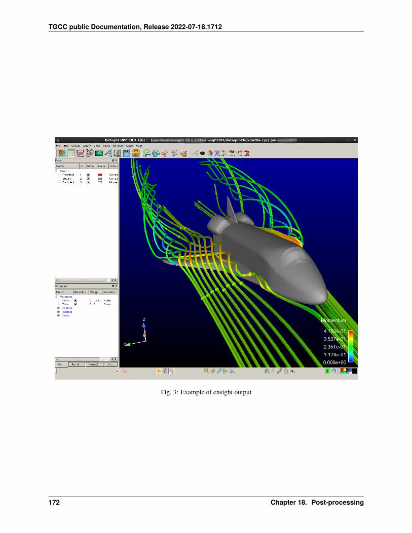
TGCC public Documentation, Release 2022-07-18.1712
Fig. 3: Example of ensight output
172 Chapter 18. Post-processing
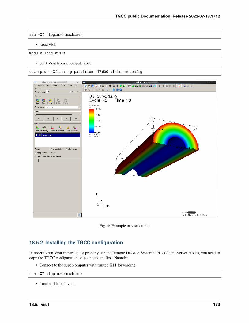
TGCC public Documentation, Release 2022-07-18.1712
ssh -XY <login>@<machine>
• Load visit
module load visit
• Start Visit from a compute node:
ccc_mprun -Xfirst -p partition -T3600 visit -noconfig
Fig. 4: Example of visit output
18.5.2 Installing the TGCC configuration
In order to run Visit in parallel or properly use the Remote Desktop System GPUs (Client-Server mode), you need tocopy the TGCC configuration on your account first. Namely:
• Connect to the supercomputer with trusted X11 forwarding
ssh -XY <login>@<machine>
• Load and launch visit
18.5. visit 173
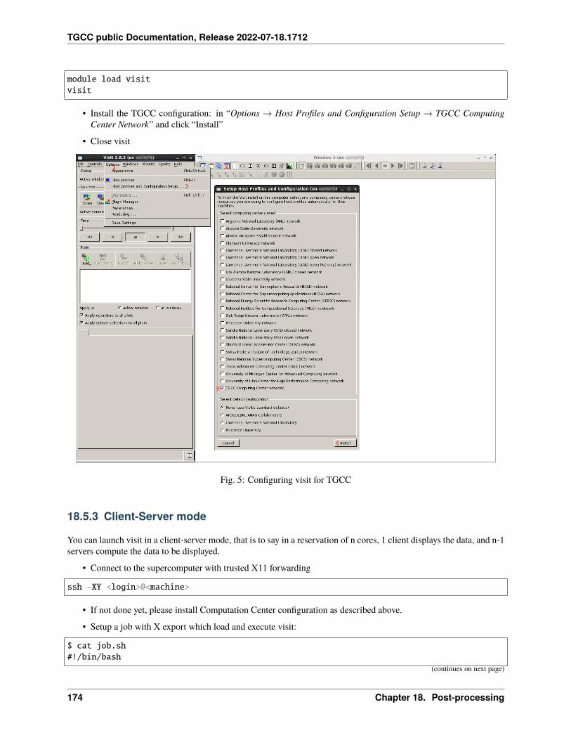
TGCC public Documentation, Release 2022-07-18.1712
module load visitvisit
• Install the TGCC configuration: in “Options → Host Profiles and Configuration Setup → TGCC ComputingCenter Network” and click “Install”
• Close visit
Fig. 5: Configuring visit for TGCC
18.5.3 Client-Server mode
You can launch visit in a client-server mode, that is to say in a reservation of n cores, 1 client displays the data, and n-1servers compute the data to be displayed.
• Connect to the supercomputer with trusted X11 forwarding
ssh -XY <login>@<machine>
• If not done yet, please install Computation Center configuration as described above.
• Setup a job with X export which load and execute visit:
$ cat job.sh#!/bin/bash
(continues on next page)
174 Chapter 18. Post-processing
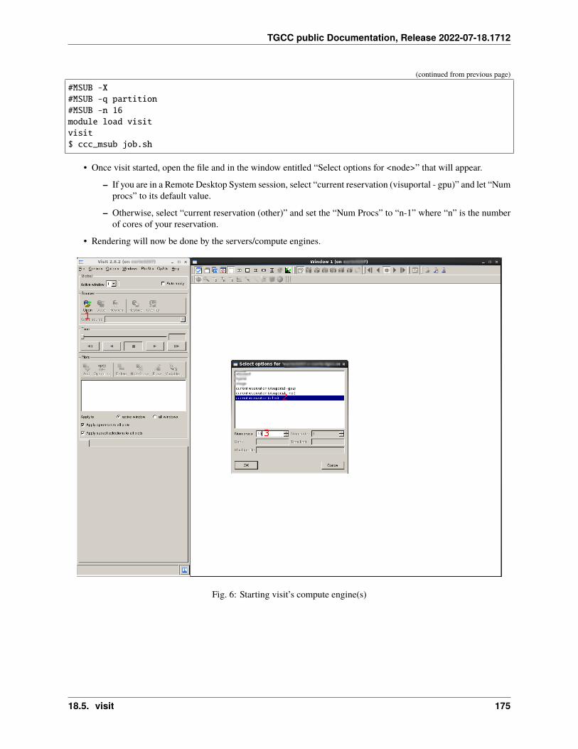
TGCC public Documentation, Release 2022-07-18.1712
(continued from previous page)
#MSUB -X#MSUB -q partition#MSUB -n 16module load visitvisit$ ccc_msub job.sh
• Once visit started, open the file and in the window entitled “Select options for <node>” that will appear.
– If you are in a Remote Desktop System session, select “current reservation (visuportal - gpu)” and let “Numprocs” to its default value.
– Otherwise, select “current reservation (other)” and set the “Num Procs” to “n-1” where “n” is the numberof cores of your reservation.
• Rendering will now be done by the servers/compute engines.
Fig. 6: Starting visit’s compute engine(s)
18.5. visit 175
TGCC public Documentation, Release 2022-07-18.1712
18.6 paraview
18.6.1 Interactive mode
You can use Paraview from a Remote Desktop System Session or from a compute node (please avoid login nodes)
To start Paraview from a Remote Desktop System session:
• Start your Remote Desktop System session
• Open a terminal
module load paraviewparaview
To start Paraview on a compute node:
• Log into the login node, with X redirection and thrusted X11 forwarding
ssh -XY login@login-node
• Find Paraview:
module load paraview
• Start Paraview from an exclusive compute node:
ccc_mprun -Xfirst -x -Q normal -p partition paraview
176 Chapter 18. Post-processing
CHAPTER
NINETEEN
VIRTUALISATION
19.1 PCOCC
PCOCC (pronounced peacock) stands for Private Cloud On a Compute Cluster. It allows users to launch containersas well as to host clusters of VMs (Virtual Machines) on compute nodes. This can be used to facilitate deploymentof applications by packaging them as container images or virtual appliances, or to setup custom environments fordevelopment or test purposes. Container images built with popular tools such as Docker or Podman can be launchedinteractively or within Slurm jobs. Clusters of VM can be instanciated on the fly with a single command which allocatesthe necessary resources to host the virtual machines, including private Ethernet and/or InfiniBand networks, createstemporary disk images from the selected templates (using CoW) and instantiates as many virtual machines as required.Facilities are provided to replicate the host environment and access user directories from the VMs or to create new VMtemplates from scratch.
19.2 Containers
The PCOCC tool allows to run containers on HPC clusters. It supports container images in Docker and OCI formats. Ina typical workflow, users first build their container images on their local workstation before importing them to a pcoccimage repository on the compute cluster. They can then spawn containers from these images, to run, for example, dataanalysis tools or parallel computations. Singularity users must translate their recipies to Dockerfile then generate animage as follow.
This can be done with the following steps:
1. On your local workstation, export a Docker image in tar archive format
$ docker save my_docker_image -o my_docker_image.tar
2. Copy the resulting tar file (here: my_docker_image.tar) to the HPC cluster, using, for example, scp or rsync
3. Import the container image (in the docker-archive tar) to your pcocc image repository on the HPC cluster:
$ pcocc image import docker-archive:my_docker_image.tar my_docker_image
4. Check that the image is now available in your repository:
$ pcocc image list
5. Launch containers from your image (this step can be repeated as needed without re-importing the image):
When starting a container from a PCOCC image, the behaviour is similar as with Docker: the task that is executed inthe container depends on whether an entrypoint or cmd has been defined when building the container image (refer to theDocker documentation for detailed explanations). Host environment variables are also not propagated to the container
177
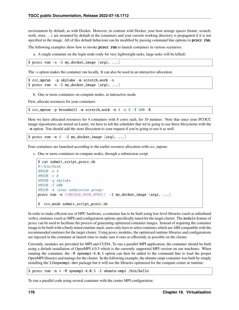
TGCC public Documentation, Release 2022-07-18.1712
environment by default, as with Docker. However, in contrast with Docker, your host storage spaces (home, scratch,work, store . . . ) are mounted by default in the containers and your current working directory is propagated if it is notspecified in the image. All of this default behaviour can be modified by passing command line options to pcocc run.
The following examples show how to invoke pcocc run to launch containers in various scenarios:
a. A single container on the login node (only for very lightweight tasks, large tasks will be killed)
$ pcocc run -s -I my_docker_image [arg1, ...]
The -s option makes the container run locally. It can also be used in an interactive allocation:
$ ccc_mprun -p skylake -m scratch,work -s$ pcocc run -s -I my_docker_image [arg1, ...]
b. One or more containers on compute nodes, in interactive mode
First, allocate resources for your containers
$ ccc_mprun -p broadwell -m scratch,work -n 4 -c 8 -T 600 -K
Here we have allocated resources for 4 containers with 8 cores each, for 10 minutes. Note that since your PCOCCimage repositories are stored on Lustre, we have to tell the scheduler that we’re going to use these filesystems with the-m option. You should add the store filesystem to your request if you’re going to use it as well.
$ pcocc run -n 4 -I my_docker_image [arg1, ...]
Four containers are launched according to the earlier resource allocation with ccc_mprun.
c. One or more containers in compute nodes, through a submission script
$ cat submit_script_pcocc.sh#!/bin/bash#MSUB -n 4#MSUB -c 8#MSUB -q skylake#MSUB -T 600#MSUB -A <your submission group>pcocc run -n ${BRIDGE_MSUB_NPROC} -I my_docker_image [arg1, ...]
$ ccc_msub submit_script_pcocc.sh
In order to make efficient use of HPC hardware, a container has to be built using low-level libraries (such as infinibandverbs), runtimes (such as MPI) and configuration options specifically tuned for the target cluster. The module feature ofpcocc can be used to facilitate the process of generating optimized container images. Instead of requiring the containerimage to be built with a finely tuned runtime stack, users only have to select runtimes which are ABI compatible with therecommended runtimes for the target cluster. Using pcocc modules, the optimized runtime libraries and configurationsare injected in the container at launch time to make sure it runs as efficiently as possible on the cluster.
Currently, modules are provided for MPI and CUDA. To run a parallel MPI application, the container should be builtusing a default installation of OpenMPI 4.0.5 which is the currently supported MPI version on our machines. Whenrunning the container, the -M openmpi-4.0.5 option can then be added to the command line to load the properOpenMPI libraries and tunings for the cluster. In the following example, the ubuntu-ompi container was built by simplyinstalling the libopenmpi-dev package but it will use the libraries optimized for the compute center at runtime:
$ pcocc run -n 4 -M openmpi-4.0.5 -I ubuntu-ompi /bin/hello
To run a parallel code using several container with the center MPI configuration:
178 Chapter 19. Virtualisation
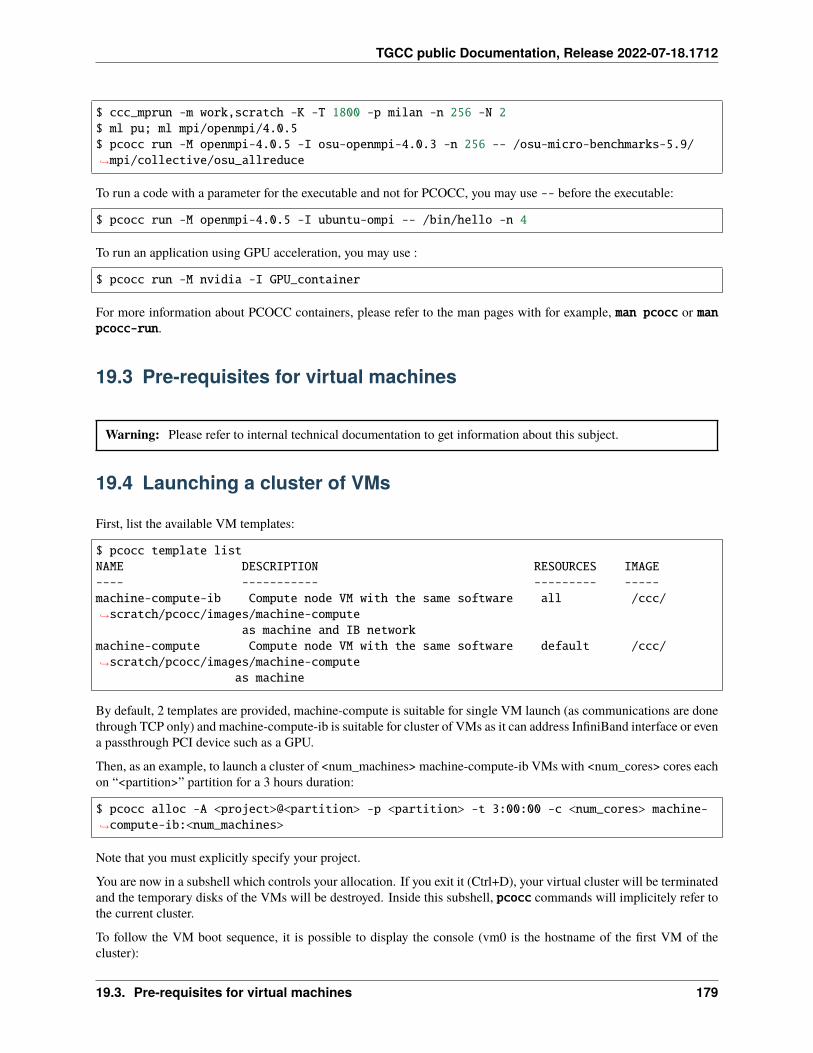
TGCC public Documentation, Release 2022-07-18.1712
$ ccc_mprun -m work,scratch -K -T 1800 -p milan -n 256 -N 2$ ml pu; ml mpi/openmpi/4.0.5$ pcocc run -M openmpi-4.0.5 -I osu-openmpi-4.0.3 -n 256 -- /osu-micro-benchmarks-5.9/→˓mpi/collective/osu_allreduce
To run a code with a parameter for the executable and not for PCOCC, you may use -- before the executable:
$ pcocc run -M openmpi-4.0.5 -I ubuntu-ompi -- /bin/hello -n 4
To run an application using GPU acceleration, you may use :
$ pcocc run -M nvidia -I GPU_container
For more information about PCOCC containers, please refer to the man pages with for example, man pcocc or manpcocc-run.
19.3 Pre-requisites for virtual machines
Warning: Please refer to internal technical documentation to get information about this subject.
19.4 Launching a cluster of VMs
First, list the available VM templates:
$ pcocc template listNAME DESCRIPTION RESOURCES IMAGE---- ----------- --------- -----machine-compute-ib Compute node VM with the same software all /ccc/→˓scratch/pcocc/images/machine-compute
as machine and IB networkmachine-compute Compute node VM with the same software default /ccc/→˓scratch/pcocc/images/machine-compute
as machine
By default, 2 templates are provided, machine-compute is suitable for single VM launch (as communications are donethrough TCP only) and machine-compute-ib is suitable for cluster of VMs as it can address InfiniBand interface or evena passthrough PCI device such as a GPU.
Then, as an example, to launch a cluster of <num_machines> machine-compute-ib VMs with <num_cores> cores eachon “<partition>” partition for a 3 hours duration:
$ pcocc alloc -A <project>@<partition> -p <partition> -t 3:00:00 -c <num_cores> machine-→˓compute-ib:<num_machines>
Note that you must explicitly specify your project.
You are now in a subshell which controls your allocation. If you exit it (Ctrl+D), your virtual cluster will be terminatedand the temporary disks of the VMs will be destroyed. Inside this subshell, pcocc commands will implicitely refer tothe current cluster.
To follow the VM boot sequence, it is possible to display the console (vm0 is the hostname of the first VM of thecluster):
19.3. Pre-requisites for virtual machines 179
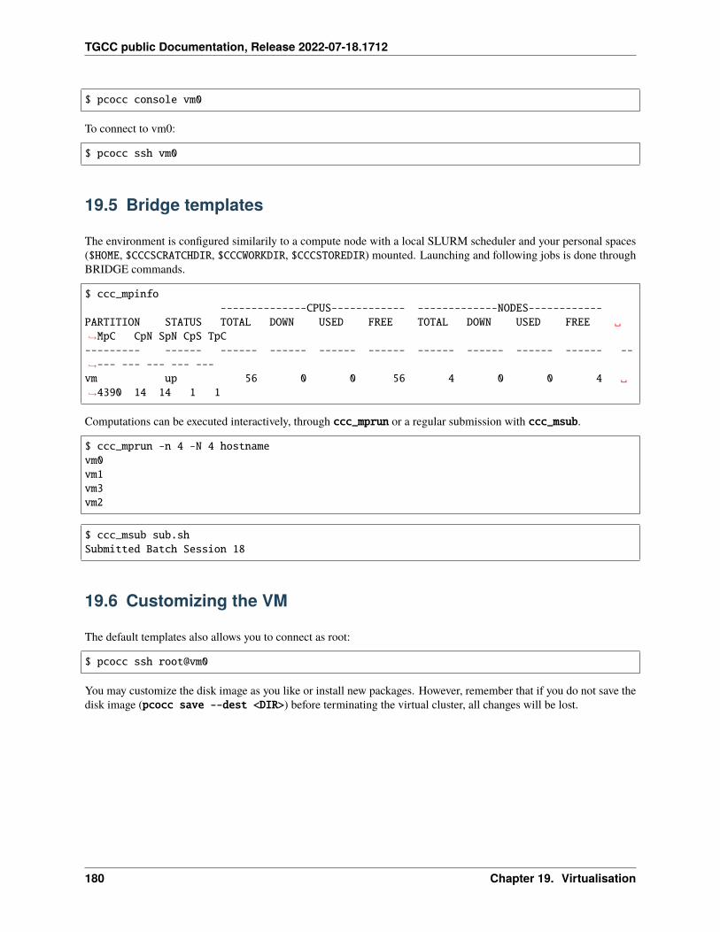
TGCC public Documentation, Release 2022-07-18.1712
$ pcocc console vm0
To connect to vm0:
$ pcocc ssh vm0
19.5 Bridge templates
The environment is configured similarily to a compute node with a local SLURM scheduler and your personal spaces($HOME, $CCCSCRATCHDIR, $CCCWORKDIR, $CCCSTOREDIR) mounted. Launching and following jobs is done throughBRIDGE commands.
$ ccc_mpinfo--------------CPUS------------ -------------NODES------------
PARTITION STATUS TOTAL DOWN USED FREE TOTAL DOWN USED FREE ␣→˓MpC CpN SpN CpS TpC--------- ------ ------ ------ ------ ------ ------ ------ ------ ------ --→˓--- --- --- --- ---vm up 56 0 0 56 4 0 0 4 ␣→˓4390 14 14 1 1
Computations can be executed interactively, through ccc_mprun or a regular submission with ccc_msub.
$ ccc_mprun -n 4 -N 4 hostnamevm0vm1vm3vm2
$ ccc_msub sub.shSubmitted Batch Session 18
19.6 Customizing the VM
The default templates also allows you to connect as root:
$ pcocc ssh root@vm0
You may customize the disk image as you like or install new packages. However, remember that if you do not save thedisk image (pcocc save --dest <DIR>) before terminating the virtual cluster, all changes will be lost.
180 Chapter 19. Virtualisation
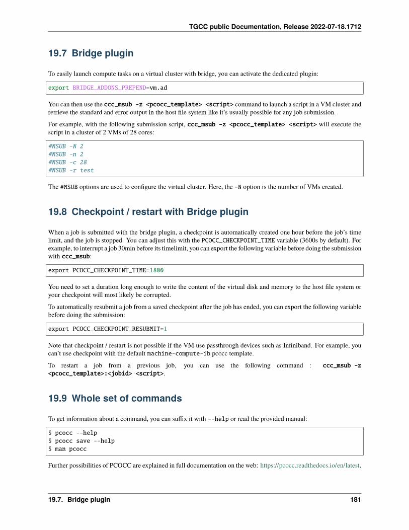
TGCC public Documentation, Release 2022-07-18.1712
19.7 Bridge plugin
To easily launch compute tasks on a virtual cluster with bridge, you can activate the dedicated plugin:
export BRIDGE_ADDONS_PREPEND=vm.ad
You can then use the ccc_msub -z <pcocc_template> <script> command to launch a script in a VM cluster andretrieve the standard and error output in the host file system like it’s usually possible for any job submission.
For example, with the following submission script, ccc_msub -z <pcocc_template> <script> will execute thescript in a cluster of 2 VMs of 28 cores:
#MSUB -N 2#MSUB -n 2#MSUB -c 28#MSUB -r test
The #MSUB options are used to configure the virtual cluster. Here, the -N option is the number of VMs created.
19.8 Checkpoint / restart with Bridge plugin
When a job is submitted with the bridge plugin, a checkpoint is automatically created one hour before the job’s timelimit, and the job is stopped. You can adjust this with the PCOCC_CHECKPOINT_TIME variable (3600s by default). Forexample, to interrupt a job 30min before its timelimit, you can export the following variable before doing the submissionwith ccc_msub:
export PCOCC_CHECKPOINT_TIME=1800
You need to set a duration long enough to write the content of the virtual disk and memory to the host file system oryour checkpoint will most likely be corrupted.
To automatically resubmit a job from a saved checkpoint after the job has ended, you can export the following variablebefore doing the submission:
export PCOCC_CHECKPOINT_RESUBMIT=1
Note that checkpoint / restart is not possible if the VM use passthrough devices such as Infiniband. For example, youcan’t use checkpoint with the default machine-compute-ib pcocc template.
To restart a job from a previous job, you can use the following command : ccc_msub -z<pcocc_template>:<jobid> <script>.
19.9 Whole set of commands
To get information about a command, you can suffix it with --help or read the provided manual:
$ pcocc --help$ pcocc save --help$ man pcocc
Further possibilities of PCOCC are explained in full documentation on the web: https://pcocc.readthedocs.io/en/latest.
19.7. Bridge plugin 181

TGCC public Documentation, Release 2022-07-18.1712
182 Chapter 19. Virtualisation
INDEX
Symbols$CCCSCRATCHDIR, 33, 180$CCCSTOREDIR, 180$CCCWORKDIR, 23, 180$CCFRWORK, 23$HOME, 33, 180$SHSPACE_MODULEFILES, 24, 40, 41$SHSPACE_MODULESHOME, 24, 40$SHSPACE_PRODUCTSHOME, 24, 40$<SHSPACE>_CCCSCRATCHDIR, 21$<SHSPACE>_CCCSTOREDIR, 21$<SHSPACE>_CCCWORKDIR, 21$<SHSPACE>_CCFRHOME, 21$<SHSPACE>_CCFRSCRATCH, 21$<SHSPACE>_CCFRSTORE, 21$<SHSPACE>_CCFRWORK, 21$<SHSPACE>_HOME, 21
BBRIDGE_MSUB_JOBID, 56BRIDGE_MSUB_MAXTIME, 56BRIDGE_MSUB_NCORE, 56BRIDGE_MSUB_NPROC, 56BRIDGE_MSUB_PWD, 56BRIDGE_MSUB_REQNAME, 56
CCCCSCRATCHDIR, 16, 23, 37CCCSHMDIR, 17CCCSTOREDIR, 16, 23, 37CCCTMPDIR, 17CCCWORKDIR, 16, 23CCFRHOME, 15CCFRSCRATCH, 16CCFRSTORE, 16CCFRTMP, 17CCFRWORK, 16
DDARSHAN_LOG_PATH, 128docdir, 25
Eenvironment variable
$CCCSCRATCHDIR, 33, 180$CCCSTOREDIR, 180$CCCWORKDIR, 23, 180$CCFRWORK, 23$HOME, 33, 180$SHSPACE_MODULEFILES, 24, 40, 41$SHSPACE_MODULESHOME, 24, 40$SHSPACE_PRODUCTSHOME, 24, 40$<SHSPACE>_CCCSCRATCHDIR, 21$<SHSPACE>_CCCSTOREDIR, 21$<SHSPACE>_CCCWORKDIR, 21$<SHSPACE>_CCFRHOME, 21$<SHSPACE>_CCFRSCRATCH, 21$<SHSPACE>_CCFRSTORE, 21$<SHSPACE>_CCFRWORK, 21$<SHSPACE>_HOME, 21BRIDGE_MSUB_JOBID, 56BRIDGE_MSUB_MAXTIME, 56BRIDGE_MSUB_NCORE, 56BRIDGE_MSUB_NPROC, 56BRIDGE_MSUB_PWD, 56BRIDGE_MSUB_REQNAME, 56CCCSCRATCHDIR, 16, 23, 37CCCSHMDIR, 17CCCSTOREDIR, 16, 23, 37CCCTMPDIR, 17CCCWORKDIR, 16, 23CCFRHOME, 15CCFRSCRATCH, 16CCFRSTORE, 16CCFRTMP, 17CCFRWORK, 16DARSHAN_LOG_PATH, 128docdir, 25FFTW3_CFLAGS, 83FFTW3_LDFLAGS, 83HOME, 15, 37I_MPI_CC, 89I_MPI_CXX, 89I_MPI_F77, 89
183
TGCC public Documentation, Release 2022-07-18.1712
I_MPI_FC, 89incdir, 25KMP_AFFINITY, 90LD_LIBRARY_PATH, 43LD_PRELOAD, 93, 119libdir, 25MANPATH, 33MKL_XXX, 82name, 78, 79OMP_NUM_THREADS, 53, 82, 157OMPI_CC, 89OMPI_CXX, 89OMPI_F77, 89OMPI_FC, 89OMPI_MCA_xxxxx, 87OWN_HOME, 21OWN_SCRATCHDIR, 21PATH, 24, 33, 40, 43PCOCC_CHECKPOINT_TIME, 181prefix, 25PROG_DOCDIR, 25PROG_INCDIR, 25PROG_LIBDIR, 25PROG_ROOT, 25SCALAPACK_XXX, 82SCOREP_EXPERIMENT_DIRECTORY, 137, 141, 143SHSPACE_INPUTDIR, 24, 40SHSPACE_MODULEFILES, 24, 40SHSPACE_MODULESHOME, 24, 40SHSPACE_PRODUCTSHOME, 24, 40SHSPACE_RESULTDIR, 24, 40TAU_CALLPATH, 161TAU_MAKEFILE, 160TAU_PROFILE, 161TAU_TRACE, 161THECODE_CFLAGS, 43THECODE_INCDIR, 43THECODE_LDFLAGS, 43THECODE_LIBDIR, 43THECODE_ROOT, 43VALGRIND_PRELOAD, 119VARNAME, 26, 43
FFFTW3_CFLAGS, 83FFTW3_LDFLAGS, 83
HHOME, 15, 37
II_MPI_CC, 89I_MPI_CXX, 89I_MPI_F77, 89
I_MPI_FC, 89incdir, 25
KKMP_AFFINITY, 90
LLD_LIBRARY_PATH, 43LD_PRELOAD, 93, 119libdir, 25
MMANPATH, 33MKL_XXX, 82
Nname, 78, 79
OOMP_NUM_THREADS, 53, 82, 157OMPI_CC, 89OMPI_CXX, 89OMPI_F77, 89OMPI_FC, 89OMPI_MCA_xxxxx, 87OWN_HOME, 21OWN_SCRATCHDIR, 21
PPATH, 24, 33, 40, 43PCOCC_CHECKPOINT_TIME, 181prefix, 25PROG_DOCDIR, 25PROG_INCDIR, 25PROG_LIBDIR, 25PROG_ROOT, 25
SSCALAPACK_XXX, 82SCOREP_EXPERIMENT_DIRECTORY, 137, 141, 143SHSPACE_INPUTDIR, 24, 40SHSPACE_MODULEFILES, 24, 40SHSPACE_MODULESHOME, 24, 40SHSPACE_PRODUCTSHOME, 24, 40SHSPACE_RESULTDIR, 24, 40
TTAU_CALLPATH, 161TAU_MAKEFILE, 160TAU_PROFILE, 161TAU_TRACE, 161THECODE_CFLAGS, 43THECODE_INCDIR, 43
184 Index
TGCC public Documentation, Release 2022-07-18.1712
THECODE_LDFLAGS, 43THECODE_LIBDIR, 43THECODE_ROOT, 43
VVALGRIND_PRELOAD, 119VARNAME, 26, 43
Index 185


