The 2000 Cape Sable Sparrow AnnualReport

Edited by

Stuart L. Pimm

Professor of Conservation Biology

Columbia University

Table of contents

Introduction

Chapter 1.

The recovery of the Cape Sable seaside sparrow through restoration of theEverglades ecosystem.

Chapter 2.

Range-wide risks to large populations: the Cape Sable sparrow as a case history

Chapter 3

Demography of the Cape Sable seaside sparrow within Everglades National Park

Chapter 4

Demonstrating the destruction of the habitat of the Cape Sable seaside sparrow

Chapter 5:

The 2000 Cape Sable sparrow census

Introduction

For the last two years, we chose to put our annual report on our work on theCape Sable sparrow on the web to facilitate discussion and to provide theinformation needed by those who make management decisions about thisendangered bird and the ecosystem on which it depends.

The set of all three years (1998, 1999, and 2000) provides a comprehensivearchive of our work.

This year the web page will likely be delayed for a few weeks as we transfer thematerials from the home of the reports for the previous two years

http://web.utk.edu/~grussell/cssshtml/csss.html.

to their new home at the Center for Environmental Research and Conservation(Check the personal web page of Professor Stuart Pimm atwww.cerc.colubia.edu.) The first version of this report is being produced inAdobe Acrobat format and distributed by e-mail. Until the new web site iscomplete, this year's report may requested in this form fromStuartPimm@aol.com.

First time readers

The materials for these three annual reports were produced sequentially. Aswith all research, we obtain new information each year, sometimes modifyingour interpretations as the new data require. Working through all this materialcan be daunting, so we offer some simple recommendations for navigation.

As a first step, read The recovery of the Cape Sable seaside sparrow through restorationof the everglades ecosystem by

Lockwood, J. and T. Fenn. 2000. The recovery of the Cape Sable seaside sparrowthrough restoration of the everglades ecosystem. Endangered Species Update.

This paper by Professor Lockwood and her colleague provides a short, succinctsummary of the ecology of this species. It appears as chapter 1 of this report.

Second, read

Curnutt, J. L., A. L. Mayer, T. M. Brooks, L. L. Manne, O. L. Bass, Jr., D. M.Fleming, M. P. Nott and S. L. Pimm. 1998. Population dynamics of theendangered Cape Sable seaside-sparrow. Animal Conservation 1:11–20.

And

Nott, M. P., O. L. Bass, Jr., D. M. Fleming, S. E. Killeffer, N. Fraley, L. Manne, J. L.Curnutt, T. M. Brooks, R. Powell and S. L. Pimm. 1998. Water levels, rapid

vegetational changes, and the endangered Cape Sable seaside-sparrow.Animal Conservation 1:21–29.

These pairs of papers deal with the demography of the sparrow and causes of itsdecline up to the 1997 field season. They appear in the 1998 report.

Finally,

Lockwood, J.L. K.H. Fenn, J.L. Curnutt, D. Rosenthal, K.L. Balent and A.L.Mayer. 1997. Life history of the endangered Cape Sable seaside sparrow.Wilson Bulletin 109(4): 720-731.

This paper provides an early overview of the sparrow's breeding biology, thegeneral features of which have not been changed by another four years offieldwork (though the details certainly have.) It, too, appears in the 1998 report.

You should now considered yourself a veteran reader and progress to the nextstep.

Veteran readers

The previous two annual reports contain chapters comparable to this one in thatthey update the papers published in international peer-reviewed journalsdiscussed in the previous section. In addition, they contain manuscripts were inpreparation at the time but that have now been accepted for publication (or willlikely be submitted in the near term.)

The work on the sparrow's risk of extinction that first appeared in Balancing onthe Brink (see the 1998 report), and as Pimm and Bass (in preparation) in the 1999report, appears here as chapter 2. It should be quoted as:

Pimm, S. L. and O. L. Bass, Jr. (in press). Range-wide risks to large populations:the Cape Sable sparrow as a case history. In Beissinger, S. and D. R.McCullough, Population Viability Analysis, The University of Chicago Press.

Professor Lockwood and her colleagues have produced updates of their work onthe bird's demography in the annual reports subsequent to their paper. Andthere have been brief mentions of the banding efforts led by Mr. David Okines.Banding and nesting studies of rare species take many years to acquire sufficientsample sizes. Chapter 3 is our first effort to summarize these efforts forpublication since 1997. This work has been submitted but not yet accepted. Itshould be quoted as:

Lockwood, J. L., Fenn, K. H., Caudill, J.M., Okines, D., Bass, O. L. jr., Duncan, J.R. and S. L. Pimm (in prep). Demography of the Cape Sable seaside sparrowwithin Everglades National Park

The work undertaken by Professor Robert Powell and Mr. Clinton Jenkinsemploying remote census technologies to modelling the changes in sparrow

habitat has produced color imagery in several papers and in previous reports.This year the work is near completion and appears as Chapter 4. Although thepaper has not yet been submitted, it should be quoted as:

Jenkins, C. N., Powell, R., Bass, O. L. Jr. and S. L. Pimm (in prep.) Demonstratingthe destruction of the habitat of the Cape Sable seaside sparrow.

This paper contains this year's most important result and we abstract theintroductory material here for emphasis.

Countries differ in the vigor to which they protect biodiversity and in theparticular laws they pass to do so. In the United States of America, one ofthe more effective laws is the Endangered Species Act. It prohibits directtake — the killing or harming — of Federally-listed endangered species.From its inception there has also been the implication that it prohibits takeindirectly — through the destruction of the ecosystems on which speciesdepend. That provision was challenged in a legal case, Sweet Homeversus Babbitt, argued in front of the Supreme Court of the United States,on February 17th 1995. In the particular context of the Spotted Owl, anOregon group challenged the responsible cabinet member, Secretary ofthe Interior Babbitt, arguing that only direct take violated the law and nothabitat destruction. In a brief of Amici Curiae scientists, one of us (Pimm)and others (Cairns et al. 1995) argued that habitat destruction is mostoften the cause of species endangerment and extinction.

The Supreme Court agreed with that position. In doing so, they raise ascientific question that transcends national boundaries: how are we todemonstrate that human actions harm the habitat on which a speciesdepends? In the case of the owl, the action — extensive logging of the oldgrowth forests on which the birds depend — was obvious. Of course, itneed not be.

Our particular concern is the Federally-listed Cape Sable seaside sparrow(Ammodramus maritimus mirabilis) a bird found only within the seasonallyflooded marshes in the Everglades of South Florida. In previouspublications, we demonstrated that the unnatural flooding of its breedinghabitat directly caused its precipitous decline in the western half of itsrange (Curnutt et al. 1998, Nott et al. 1998). The flooding resulted fromthe diversion of the area’s drainage, Shark River Slough, to the west of itsnatural path and a change in the timing of its seasonal ebb and flow.Concomitant with those changes, areas in the east became over-drainedand more susceptible to anthropogenic fires. Those fires also harm thebirds directly.

We left open the possibility that flooding and fires also damaged thehabitat and so the birds as a consequence. In this paper, we willdemonstrate that flooding has indeed altered the habitat in which thesparrow occurs, done so in a way to preclude the bird’s use of the habitat,and over a period of years longer than the flooding itself.

The paper proceeds in two stages. The first explains how we predictsparrow habitat. The second stage is an evaluation of those predictions.

We will present two key results.

(1) Across the eight years of the study, large year-to-year fluctuations inpredicted habitat confirm the culpability of water managers. Flooding in1993 and 1995 greatly reduced the habitat predicted to be suitable for thesparrow compared to 1992.

(2) The predicted suitable habitat west of Shark River Slough was at a lowebb in 1995 and has recovered slowly, but consistently, in the years fromthen until 1999. This formal, technical demonstration matches exactly thesubjective opinion expressed by Bass and Pimm from their visual surveys.By 1999, the predicted suitable habitat had not yet recovered to its pre-flood state. The habitat is recovering faster than the slowly recoveringbird populations. It is the repetition of precisely such a scenario that wepredict could lead to the species’ extinction (Pimm and Bass, 2000).

Lest the significance of this text still be unclear, let us be blunt. We do not issueopinions of biological jeopardy under the provisions of the Endangered SpeciesAct: the Fish and Wildlife Service does. But in this text is an explicitrecommendation. In addition to harming the birds directly, water managershave damaged them indirectly by destroying essential habitat over a large areaand over many years.

The final chapter, (5), arises from the recommendations of the Walter's committee(see the 1999 report) that we repeat the annual helicopter census of the species toobtain an estimate of the accuracy of the survey methods. We tried to implementsuch a count in 1999, but unaccountable delays in establishing the Walter'scommittee meant that the second survey was much later in the breeding seasonthan the first. For reasons we understand, the two surveys were not replicates.This year, the surveys were completed within the same period at the height ofthe nesting season. Chapter 5's remarkable claim is that the surveys are indeedreplicates of each other and that the survey provides an unbiased and efficientsampling of the population.

Please take note of the following advisory. We make this report available soonafter the completion of each year's field season to facilitate discussion and tohelp managers make the best possible choices.

The material presented here, unless it has alreadybeen published, appears here in draft form.

Chapter 1.

The recovery of the Cape Sable seaside sparrow throughrestoration of the Everglades ecosystem.

Julie L. Lockwood

Department of Environmental Studies, Natural Sciences II, University ofCalifornia, Santa Cruz, CA 95064; lockwood@cats.ucsc.edu

Katherine H. Fenn

Department of Ecology and Evolutionary Biology, 569 Dabney Hall, Universityof Tennessee, Knoxville, TN 37996; tfenn@ix.netcom.com.

Abstract

The Cape Sable seaside sparrow (Ammodramus maritimus mirabilis) has beenlisted as federally endangered since 1967. Its small population size and unique ecologyhave perpetuated conservation concern. The ultimate factor in this sub-species’ decline isthe alteration of the everglades ecosystem. Range-wide surveys conducted since 1992have documented 90 percent declines within some sub-populations leaving the sub-species vulnerable to extinction in the near future. Although the life history of thesparrow is typical of grassland birds, its demographic characteristics leave it highlyvulnerable to even short-term alterations of fire and flood regimes. A multi-billion dollarrestoration plan has been launched in an effort to return everglades’ hydrology to a morenatural state. However, even with this plan, the Cape Sable seaside sparrow is in dangerof extinction. As shown for the plight of the Dusky seaside sparrow (Ammodramusmaritimus nigrescens), a close and now extinct relative of the Cape Sable seasidesparrow, management actions must be swift to avert the extinction of short-lived, habitatspecialists such as this sparrow.

Introduction

Cape Sable seaside sparrow (Ammodramus maritimus mirabilis) populationnumbers have declined nearly 50 percent between 1992 and 1996 (Curnutt et al.1998). This federally listed sub-species currently exists within the protectedlands of Everglades National Park (ENP) and adjacent Big Cypress NationalPreserve. These two biological preserves (together nearly 8,500 km2 in area) formone of the largest protected areas in North America, yet fail to function as apreserve for this and many other inhabitants (Mayer and Pimm 1998). Becauselarge-scale hydrologic changes reflect patterns of population decline in the Cape

Sable seaside sparrow, this bird is perceived to be the ‘canary’ in the ‘coal mine’of the everglades. At present, the 20-year plan to restore original evergladeshydrology promises recovery of the ecosystem. For short–lived species such asthe sparrow; however, special attention must be paid to interim protection.

Historical perspective

Historically, the everglades were a ‘river of grass’ encompassing an estimated28,205 km2 of unbroken, freshwater prairie (Mayer and Pimm 1998). Extendingfrom Lake Okeechobee in the north to Florida and Biscayne Bays in the south,water drained across the flat terrain as a ‘sheet,’ its peak averaging 64 km wideand 0.5 m in depth (Mayer and Pimm 1998). The heaviest flows (up to sixkm/hr) occurred during the wet-season (June to January).

South Florida was sparsely populated before the turn of the century (Tebeau1968). High variation in water flow made south Florida an unpredictable placefor most economic ventures, especially commercial farming (Mayer and Pimm1998, Snyder and Davidson 1994). In 1850 the U.S. Congress passed the SwampLands Act which encouraged development in south Florida by ‘reclaiming’flooded lands for agriculture (Light and Dineen 1994). This act, and anotherpassed in 1948 (the Central and South Florida Project), set in motion a series ofhydrology changes culminating in the construction of 2,200 km of canals andlevees and over 40 pumps and spillways (Mayer and Pimm 1998). LakeOkeechobee was impounded in the 1930s, permanently altering the hydrologiclink between the lake and the freshwater prairies to the south (Light and Dineen1994).

These changes enabled south Florida to become one of the largest producers ofwinter vegetables and domestic sugarcane in North America (Snyder andDavidson 1994). Coupled with flood control, economic growth enabled thehuman population to reach four million by 1990 (Light and Dineen 1994). Asearly as the 1940s, officials recognized that this growth created additionaldemands on available water. Consequently, three Water Conservation Areas(WCAs) were included in flood control measures and established just north ofENP (Figure 1). These areas receive most of the run-off from Lake Okeechobeeand the Everglades Agricultural Areas. They provide freshwater sources foragriculture, residential areas, and recreation. They also function as a ‘filter’removing agricultural run-off (e.g., phosporous) from water entering naturalareas such as ENP (Light and Dineen 1994).

Between the WCAs and federal biological preserves, 67 percent of the originaleverglades ecosystem is protected from urban development. Although nearlyhalf of that area is managed largely for biological resources, there is a limit topreservation efforts as only the lands, not the historical water flows, wereprotected. Since the re-plumbing of south Florida, water flows from the WCAsinto the principle tributary of the lower everglades (Shark River Slough) via sixspillways (Figure 1). Levees split the slough into eastern and western halves(Light and Dineen 1994). Western Shark River Slough receives most of the water,while the eastern slough (and other eastern tributaries such as Taylor Slough)

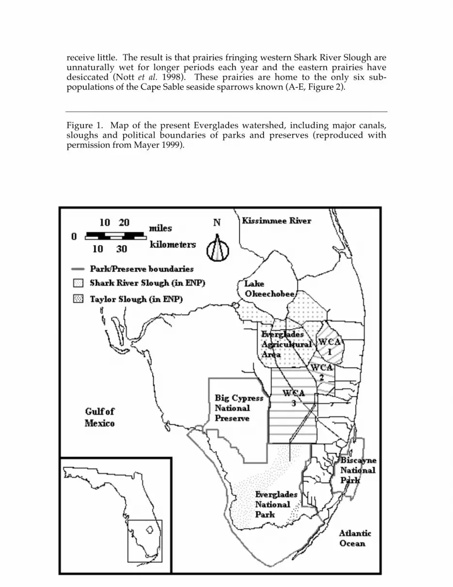
receive little. The result is that prairies fringing western Shark River Slough areunnaturally wet for longer periods each year and the eastern prairies havedesiccated (Nott et al. 1998). These prairies are home to the only six sub-populations of the Cape Sable seaside sparrows known (A-E, Figure 2).

Figure 1. Map of the present Everglades watershed, including major canals,sloughs and political boundaries of parks and preserves (reproduced withpermission from Mayer 1999).

Figure 2. Location of Cape Sable seaside sparrow sub-populations withinEverglades National Park and Big Cypress National Preserve.

The Cape Sable seaside sparrow, a small, drably colored bird, has never beencommon (Curnutt et al. 1998). First described in 1919 by Arthur Howell, this sub-species was thought to exist only within the freshwater marshes that grew on

Sha

rk R

iver

Slo

ugh

A

B

C

D

E

F

Met

ropo

litan

Mia

mi

ENP Boundary

EN

P B

oundary

EN

P B

oundary

ENP Boundary

ENP Bou

ndar

y

Florida Bay

ENP Boundary

6 km

N

Cape Sable early this century (Werner and Woolfenden 1983). A hurricane thatmade landfall over Cape Sable on September 2, 1935, forever changed the Cape’svegetation and landscape (Mayer and Pimm 1998, Curnutt et al. 1998). Thesparrow was not found on Cape Sable after that event. In fact the species wasbelieved extinct until L.A. Stimson’s 1951 documentation of inland populationsin freshwater prairies (Stimson 1956). Because most seaside sparrows live withintidal marshes, this discovery made the sub-species an ecological oddity (Post andGreenlaw 1994). As a likely consequence of the sparrow’s phoenix-like identityand its unusual ecology, the U.S. Congress placed the Cape Sable seasidesparrow on the first endangered species list enacted in 1967 (Curnutt et al. 1998).

Current status

In 1981, ENP researchers conducted range-wide point counts of the Cape Sableseaside sparrow breeding population. Points were located one km apart andaccessed via helicopter (Kushlan and Bass 1983). This survey yielded sparrowpopulation estimates of over 6,000 individuals, with more than 2,000 located ineach of two ‘core’ sub-populations (A and B) (Kushlan and Bass 1983). Similarestimates resulted from the next survey in 1992. In 1993, however, estimatesdropped 90 percent from 2,500 to 400 individuals within sub-population A(Curnutt et al. 1998). Sub-populations C, D, and F each declined from over 400individuals to fewer than 80 in the ensuing years (Curnutt et al. 1998). Annualsurveys since 1993 have shown no reverse in these declines (Pimm and Bass1999). Only the central sub-populations (B and E) contain relatively stablenumbers from year to year.

To understand these declines, we have monitored nests and color-bandedindividuals from nine study plots (each 0.50 km2) within sub-populations A, Band E (Lockwood et al. 1999a,b). From six years of study, we know the followingaspects of the sparrow’s demography. The breeding season can last from lateMarch to August depending on the onset of summer rains (Lockwood et al. 1997,Werner 1975). A pair can fledge at least three broods per breeding season withearly broods more likely to fledge young than later broods (40 percent vs. 16percent Mayfield success scores respectively). Sparrows prefer to nest in one mtall sparse sawgrass (Cladium jamaicense) stands mixed with bunchgrasses typicalof seasonally dry areas (Lockwood et al. 1999b). Nests are built approximately 16cm from the soil surface with a standard variation in height off the groundbetween 2 and 30 cm (Lockwood et al. 1999a, Werner 1975). Adults feednestlings grasshoppers, spiders, dragonflies, and lepidoptera larvae, all locallyabundant food sources (Lockwood et al. 1997). The principle threat to nests ispredation, probably by water snakes or rats (Lockwood et al. 1997).

Adults are site-fidelic, often returning to the same 200 m territory every year tobreed (Lockwood et al. 1999a). When sparrows are not breeding they do nottravel far. Using radio telemetry, Dean and Morrison (1998) recorded sporadiclong distance movement over five km, but most tagged individuals stayedwithin one km of their nesting grounds. We have never re-sighted an individualbanded in one sub-population within another (Lockwood et al. 1999a). Adultsparrows live a maximum of four years and just less than half of the adults in

any given year will die (Lockwood et al. 1999a). Hatch-year individuals exhibitlow survival their first year out of the nest but they are more likely to move overlonger distances (up to one km) (Lockwood et al. 1999a).

Although these demographic attributes are typical of most grassland birds, theybecome a unique liability in the context of current alterations in everglades waterflow. In the western prairies of ENP, satellite images and ground-basedhydrologic monitoring stations show several high water events between 1993and 1996. In some years, water levels reached 50 cm above ground level (Nott etal. 1998). This exceeds the average nest height off ground by 34 cm and thehighest nest ever recorded by 20 cm. These large water flows did not result fromrainfall per se, but were due to released WCA water (Nott et al. 1998).

In the eastern prairies, altered hydrology has changed temporal fire patterns that,in turn, have impacted sparrow breeding habitat. Although periodic firesmaintain freshwater prairies by preventing the encroachment of shrubs andhardwood trees (Kushlan and Bass 1983), comparisons between fire records andsparrow surveys demonstrate the following: 1) sparrows regularly occupy sightsthat have burned one year prior, and 2) historically occupied areas that burnevery one or two years rarely hold sparrows today (Curnutt et al. 1998).

Since sparrows live a maximum of four years, short-term disruption ofreproduction (such as fire or flood) can significantly effect population numbers(Lockwood et al. 1999a). In areas where adult sparrows cannot breed for two orthree consecutive years, most adults die without replacing themselves in thepopulation. This situation is exacerbated by the sparrow’s limited clutch size. Apair of adult sparrows averages two young per nesting attempt. Theoretically, ifall adults in an area successfully fledge one brood, population number willsimply remain stable. (In practice, population numbers still decrease due to thelow survivorship of juveniles.) Population increases are only possible whenindividuals successfully fledge two to four broods per breeding season(Lockwood et al. 1999a).

When short-term disruptions occur over a wide geographic range, recovery isfurther hampered by the sparrow’s limited dispersal over long distances. Lownumbers will persist because immigration rarely occurs across sub-populations.There is little chance for the ‘rescue effect’ whereby individuals from a stablesub-population immigrate into a declining one.

A final concern is that high water and frequent fires are causing long-termchanges in habitat structure (Nott et al. 1998, Lockwood et al. 1999a). Known tobe a habitat specialist, this subspecies will not breed in prairies lacking specificstructural cues (Lockwood et al. 1999b).

Restoration and future management

Restoring historical ‘natural’ water flows was a goal of a bill passed by the U.S.Congress in 1992 (Mayer 1999). The restoration plan aims to rectifyenvironmental damage done by the 1948 Central and South Florida Project while

maintaining adequate flood control and freshwater supplies for the localpopulous (Governor’s Commission for a Sustainable Florida 1995). Though theplan is promising, the task is monumental. Current estimates place thecompletion of the restoration at 20 years (Mayer 1999). The existentconfiguration of canals and levees simply provides no physical route to quicklyredirect water flow from the over-flooded west to over-dry east (Pimm and Bass1999).

Given the observed steep declines in Cape Sable seaside sparrow numbers overtwo or three years, there is no guarantee the sparrow can survive the 20 requiredto restore its breeding habitat. Consider the damage its close relative, the Duskyseaside sparrow (Ammodramus maritimus nigrescens), sustained between 1960 and1980. The Dusky seaside sparrow was once found around Titusville, Florida.Like the Cape Sable seaside sparrow, the Dusky inhabited seasonally floodedmarshes and existed in distinct geographic populations. Also like the Cape Sableseaside sparrow, the Dusky declined when hydrological changes left breedinggrounds flooded or fire prone.

From an estimated 2,000 pairs on Merritt Island in the 1950s, DDT had alreadyreduced populations 70 percent by 1957 (600 pairs) (Sykes 1980, Trost 1968). Abad situation was made worse when mosquito control impoundments floodedbreeding habitat. The Dusky declined another 90 percent to 70 pairs by 1963(Sykes 1980, Trost 1968). The threat was understood and the Dusky’s habitatrequirements documented (Trost 1968). Piecemeal studies to determine whetherthe birds would respond favorably to restoration of ‘natural’ hydrologic patternssatisfied endangered species legislation (Walters 1992) but left only oneindividual on Merritt Island by 1977 (Sykes 1980, Baker 1973, Sharp 1969).

The population of Dusky seaside sparrows located in the marshes along the St.John’s river was estimated at 984 males in 1968 (Sharp 1970). Although it tooktwo years to purchase U.S. National Wildlife refuge land here for the endangeredbird, it took only one to gain a permit to build a highway through one denselypopulated colony (Walters 1992). Highways and development outside the refugereduced the largest colony from 100 to 12 birds (Baker 1978). Inside the refuge,an open ditch drained Dusky habitat while six fires from neighboring farmsburned over 4,000 acres. By 1977 fewer than a dozen birds of the 143 counted in1970 were left on the refuge (Baker 1978). Despite urgent requests for fire lines asearly as 1975, they were not completed (nor was the ditch plugged) until 1979.By that time, only nine males were left (Walters 1992). The last wild Duskyseaside sparrows were taken into captivity in 1980. The last individual, referredto as Orange for the legband he wore, died in captivity in 1987.

Conclusion

In many ways the current recovery prospects of the Cape Sable seaside sparrowmirror those of the Dusky from the early 1960s. Recovery seems feasible. Thesparrow’s demography and habitat requirements are known; the hydrologicchanges that impact that habitat are understood. Unlike the Dusky, the CapeSable seaside sparrow enjoys advantages such as higher population numbers, a

range entirely within federally protected lands, and consensus on the need torestore the ecosystem on which it depends.

Nevertheless, these advantages do not guarantee success. With such obviousparallels between the management needs of the Dusky and those of the CapeSable seaside sparrow it is incumbent upon managers to avoid the known pitfallsthat lead to extinction. More than anything else, the story of the Duskyillustrates how critical the timing of management decisions are in dealing withshort-lived habitat specialists. Each delay in decisions to purchase refuge land,construct fire lines, and seasonally drain impoundments, carried the cost of a fewmore Dusky seaside sparrows. Though the restoration of the Evergladesecosystem is a commendable and significant undertaking, it in no way alleviatesthe need for short-term, and often difficult, management actions. Without suchactions, the Cape Sable seaside sparrow may become a martyr for the threatenedecosystem about which it once raised awareness.

Literature Cited

Baker, J.L. 1978. Status of the Dusky seaside sparrow. Georgia Department ofNatural Resources Technical Bulletin Pages 94-99.

Baker, J.L. 1973. Preliminary studies of the Dusky seaside sparrow on the St.John’s National Wildlife Refuge. Proceedings of Annual ConferenceSoutheastern Association of Fame and Fish Commissioners. 27:207-214.

Curnutt, J.L. A.L. Mayer, T.M. Brooks, L. Manne, O.L. Bass Jr., D.M. Fleming,M.P. Nott, and S.L. Pimm. 1998. Population dynamics of the endangeredCape Sable seaside sparrow. Animal Conservation 1(1): 11-21

Dean, T.F. and J.L. Morrison. 1998. Non-breeding ecology of the Cape Sableseaside sparrow (Ammodramus maritimus mirabilis). 1997-1998 field seasonfinal report. U.S. Fish and Wildlife Service, South Florida EcosystemOffice, Vero Beach, FL.

Governor’s Commission for a Sustainable South Florida. 1995. A conceptualplan for the C&SF restudy. Report submitted to Governor Lawton Chiles.Coral Gables, Fl. Retrieved on 24 November, 1999:http://dlis.dos.state.fl.us/fgils/agencies/sust.tocs.htm

Kushlan, J.A. and O.L. Bass jr. 1983. Habitat use and the distribution of the CapeSable seaside sparrow. Pages 139-146 in T. Quay, J. Funderburg Jr. D.Lee, E. Potter, and C. Robbins, eds. The seaside sparrow. Its biology andmanagement. Occas. Papers of the North Carolina Biological Survey.1983-5, Raleigh, North Carolina.

Light, S.S. and J.W.Dineen. 1994. Water control in the everglades: A historicalperspective. Pages 47-84 in S.M. Davis and J.C. Ogden, eds. Everglades:The ecosystem and its restoration. St. Lucie Press, Delray Beach, Fl.

Lockwood, J.L. K.H. Fenn, J.L. Curnutt, D. Rosenthal, K.L. Balent and A.L.Mayer. 1997. Life history of the endangered Cape Sable seaside sparrow.Wilson Bulletin 109(4): 720-731.

Lockwood, J.L., K.H. Fenn, J.M. Caudill, D. Okines, and J.R. Duncan. 1999a.Demography of the Cape Sable seaside sparrow (Ammodramus maritimusmirabilis) . R e c o v e r e d o n 2 4 N o v e m b e r 1 9 9 9 :http://web.utk.edu/~grussell/cssshtml/csss.html.

Lockwood, J.L., K.H. Fenn, T.L. Warren, R. Hirsch-Jacobson, A. VanHolt, and A.Fargue. 1999b. Defining nest site microhabitat and preferences to aid inthe recovery of the Cape Sable seaside sparrow. Recovered on 24November 1999: http://web.utk.edu/~grussell/cssshtml/csss.html

Mayer, A.L.1999. Cape Sable seaside sparrow (Ammodramus maritimus mirabilis )habitat and the everglades: ecology and conservation. Ph.D. dissertationsubmitted to the University of Tennessee, Department of Ecology andEvolutionary Biology, Knoxville, TN.

Mayer, A.L., and S.L. Pimm. 1998. Integrating endangered species protectionand ecosystem management: the Cape Sable seaside sparrow as a casestudy. Pages 53-68 in G.M. Mace, A. Balmford, and J.R. Ginsberg eds.Conservation in a changing world. Cambridge University Press,Cambridge, UK.

Nott, M.P., O.L. Bass Jr., D.M. Fleming, S.E. Killeffer, N. Frahley, L. Manne, J.L.Curnutt, T.M. Brooks, R. Powell, and S.L. Pimm. 1998. Water levels,rapid vegetation changes, and the endangered Cape Sable seasidesparrow. Animal Conservation. 1(1): 23-32

Pimm, S.L. and O.L. Bass Jr. 1999. Risks in large populations: the Cape Sablesparrow as a case history. Recovered on 24 November 1999:http://web.utk.edu/~grussell/cssshtml/csss.html

Post, W. and J.S. Greenlaw. 1994. Seaside sparrow (Ammodramus maritimus).Pages 1-28 in A. Poole, and F. Gill eds. The birds of North America, No.127. Philadelphia: The Academy of Natural Sciences, Washington, D.C.:The American Ornithologists’ Union.

Sharp, B.E. Numbers, distribution and management of the Dusky SeasideSparrow. Master’s thesis, University of Wisconsin, 1968

Sharp, B.E. 1969. Conservation of the Dusky Seaside Sparrow on Merritt Island,Florida. Biological Conservation 1:175-6.

Sharp, B.E. 1970. A Population estimate of the Dusky seaside sparrow. TheWilson Bulletin 82:158-66

Snyder, G.H. and J.M. Davidson. 1994. Everglades agriculture: past, presentand future. Pages 85-116 in S.M. Davis and J.C. Ogden ed. Everglades.The ecosystem and its restoration. St. Lucie Press, Delray Beach, FL.

Stimson, L.A. 1956. The Cape Sable seaside sparrow: its former and presentdistribution. Auk 73:489-502.

Sykes, P.W. Jr., 1980. Decline and Disappearance of the Dusky Seaside sparrowfrom Merritt Island, Florida. American Birds 34(September 1980):728-737.

Tebeau, C.W. 1968. Man in the everglades: 2000 years of human history in theEverglades National park. University of Miami Press, Miami, FL.

Trost, C.H. 1968. Dusky seaside sparrow. Pages 849-859 in O.L. Austin, Jr. ed.Life Histories of North American Cardinals, Grosbeaks, Buntings,Towhees, Finches, Sparrows, and Allies by A.C. Bent. US Natural HistoryMuseum Bulletin 237.

Walters, M.J. 1992. A shadow and a song. Chelsea Green Publishing Co., PostMills VT.

Werner, H.W. and G.E. Woolfenden. 1983. The Cape Sable sparrow: its habitat,habits, and history. Pages 55-75 in T. Quay, J. Funderburg Jr. D. Lee, E.Potter, and C. Robbins, eds. The seaside sparrow. Its biology andmanagement. Occas. Papers of the North Carolina Biological Survey.1983-5, Raleigh, North Carolina.

Chapter 2.

Range-wide risks to large populations: the Cape Sablesparrow as a case history

Stuart L. Pimm

Center for Environmental Research and Conservation, Columbia University,MC5556, 1200 Amsterdam Ave. New York, NY 10027, USA

Oron L. Bass Jr.

South Florida Natural Resources Center, Everglades National Park Homestead,FL 33034, USA.

Abstract

Very small populations — those numbering a few to a few dozen breeding pairs— often go extinct quickly. The reasons for their doing so are well-understoodand relatively easy to model. Considerable experience teaches that much largerpopulations that occur across much wider ranges can become extinct quickly too.Understanding the fate of these species is the much more difficult challenge thatthis paper will address. The species of concern is the Cape Sable sparrow.

We explore two methods of calculating the sparrow's risk of extinction. The firstemploys the idea that one can characterize the natural limits of population sizefluctuations over time on the basis of past experience of the species of concern orsome similar species. So armed, one can predict whether the lower limit willencompass such low levels that rapid extinction will be probable. This is afamiliar recipe. We show that this method failed spectacularly even whenapplied to a situation where it would seem entirely appropriate. Our secondmethod identifies the causes of the sparrow's population fluctuations. Inparticular, we consider the factors the cause its range to shrink and its ability torecover from such shocks. By understanding the mechanisms underlyingpopulation fluctuations we deduce an altogether bleaker picture of the bird'sfuture.

Introduction

Very small populations — those numbering a few to a few dozen breeding pairs— often go extinct quickly. The reasons for their doing so are well understood.Such populations suffer the problems of finding suitable mates, of manyindividuals dying before the next breeding season from different causes, loss ofgenetic variability and its deleterious consequences, and other unavoidablevagaries of birth and death. The importance of these chance factors usuallydiminishes quickly as populations become larger. Nonetheless, considerableexperience teaches that much larger populations can become extinct quickly too.Indeed, we know that vertebrate populations numbering in the low thousands ofbreeding pairs are too rare to enjoy a secure future (Baillie and Groombridge1996, Collar et al. 1994, Mace 1996). Understanding the fate of these species is themuch more difficult challenge that this paper will address.

Large populations may be composed of many smaller partially isolated sub-populations. If so, the balance between frequent local extinction and re-colonization from surviving populations determines the species’ long-term fate(Hanski 1998). In such cases, the insights from studies of very small populationsare of value (Pimm et al. 1993, Pimm and Curnutt 1994). In other cases, aninexorable decline in numbers, perhaps driven by a readily observable reductionin habitat, leads to a clear prediction of a species’ demise. Yet other species maybe at risk because of the high year-to-year variability in their numbers that typifyall natural populations (Pimm 1991). In nature, many individuals die from thesame causes — bad weather, for instance. Such natural population fluctuationscan prove terminal for a species that is now more geographically restricted thanin the past.

The case history we shall present may be typical in requiring answers to all thequestions implied by the last paragraph: what is the spatial organization of thepopulation? Are any of its geographically determined sub-populationssufficiently small to warrant concerns over those “unavoidable vagaries of birthand death?” What are the unnatural causes of population decline? How willthese causes affect the population in the future? What are the natural causes ofpopulation fluctuations and how can we anticipate to what low levels they willdrive the population in the future?

The species of concern is the Cape Sable sparrow (Ammondramus maritumusmirabilis), a drab, olive-brown bird, so obscure and lacking in charisma that itwas not discovered until well into this century. First, we present some briefremarks about its natural history and about the southern Everglades to which itis restricted. These remarks summarize Lockwood et al. (1997), Curnutt et al.(1998), and Nott et al. (1998).

Next we explore two methods of calculating the sparrow's risk of extinction. Thefirst employs the idea that one can characterize the natural limits of populationsize fluctuations over time from the study of those fluctuations. So armed, onecan predict whether the lower limit will encompass such low levels that rapidextinction will be probable. This is a familiar recipe. It characterizes the papers

Brook et al.'s (2000) meta-analysis of the predictive accuracy of "populationviability analysis". One of us has devoted considerable thought to it (e.g. Pimm1991). We shall show that this method failed spectacularly even when applied toa situation where it would seem entirely appropriate. A second methodidentifies the causes of the sparrow's population fluctuations, in particular, itsrange contractions and its ability to recover from them. By understanding themechanisms underlying population fluctuations we deduce an altogether bleakerpicture of the bird's future.

The Cape Sable sparrow and the ecosystem on which it depends

The sparrow is a considered to be a subspecies of the widespread seasidesparrow, albeit an ecologically and geographically distinct one. It is not a”seaside” sparrow ecologically as it inhabits freshwater rather than saltwatermarshes. In addition to its unique habitat, it is geographically isolated. Thenearest surviving subspecies, A. m. peninsulae is 300 km to the north. Althoughfirst discovered in 1918 on Cape Sable, vegetation changes after the massivehurricane of September 1935 made the Cape unsuitable for it.

The U. S. Fish and Wildlife Service included the subspecies in the first list ofendangered species on March 11, 1967, (32 Federal Register 4001). Its restrictedrange and the fate of the population on Cape Sable were the primaryjustifications. The subsequent rapid extinction of the Dusky seaside-sparrow (A.m. nigriscens) in northern Florida lent support to that decision.

Shark River Slough is the primary drainage in the southern Everglades of Florida(see figures 1 and 2, chapter 1). To its west lies the higher ground of the BigCypress and, to the east, the Atlantic coastal ridge. Expanses of marl prairie liebetween the main drainage of Shark River Slough and these two modest ridges.In contrast to the main Slough, these prairies are inundated on average only fromthree to seven months per year. These seasonally flooded wetlands to the eastand west of the slough are the particular ecosystem on which this bird depends.

Currently, nearly all the overland flow in the Shark River Slough drainageoriginates from the four S-12 gated spillways at the northern boundary ofEverglades National Park (see figures 1 and 2, chapter 1). The east-westdistribution of these structures covers about half of the pre-drainage expanse ofShark River Slough. Historically, most of the overland flow occurred toward theeastern edge of Shark River Slough — as suggested by the figure. The S-12structures, however, are on the western edge: it across these structures that thewater actually flows.

This artificial hydrology affects the two expanses of marl prairie on either side ofthe slough in opposite ways. The western marl prairies naturally remained dryfor much of the year. They were inundated seasonally by rainfall and overflowfrom the slough. They are now subject to the vagaries of water releases from theS-12 structures.

The southeast corner of the Florida peninsula held the largest expanse of marlprairie. Bounded by the eastern edge of Shark River Slough, it spread southeast,encompassing the southern terminus of the Atlantic coastal ridge. It ended at thethin line of mangroves along the northeastern shore of Florida Bay. To the north,the marl prairies once extended in a long arm to central Dade County. Thisexpanse of potential sparrow habitat suffered two major assaults. The moredrastic was the conversion of the eastern portion of prairies to residential andagricultural lands.

Much of the remaining prairie, at and around the eastern boundary ofEverglades National Park, is over-drained and subject to frequent fires. Fires inthe wet season (June to October) are caused by lightening strikes and aregenerally small and patchy because the ecosystem is already wet. They canoccur throughout the region. Those at the end of the dry season, (March to lateMay) are frequently caused by human carelessness and tend to burn large areasalong the Everglades eastern boundary but sometimes deep into the naturalareas.

Curnutt et al. (1998) estimated that nearly half of the original prairie has beendestroyed or degraded. As for many species for which we must assess the risk ofextinction, the ultimate cause of endangerment is the massive reduction insuitable habitat.

Bass and Kushlan (1982) conducted the first extensive sparrow survey in 1981.We repeated the survey in 1992 and annually thereafter. Across a 1 km x 1 kmgrid of more than 600 sites, we record the number of sparrows seen or heardwithin a 10 minute interval. We take particular care to visit all locations thatmight hold sparrows and do not observe birds at most of the sites we survey.This suggests that we do not miss many (if any) sites that hold birds.

To estimate the actual numbers of sparrows from the number we observed onour survey, we multiply each singing male by 16. This correction is based on therange at which we can detect the sparrow’s distinctive song — it encompasses1/8 th of a square kilometer — and on the assumption that one femaleaccompanies each singing male. Work on our intensive study plots confirms thiscalibration (Curnutt et al. 1998).

Using this calibration, we estimated that the total population of this species wasover 6000 in both 1981 and 1992. The birds are not distributed continuously, butare grouped into six sub-populations of varying sizes (see figure 2, chapter 1)).Sub-population A (west of Shark River Slough) was the most numerous in 1981(~2700 birds) and B held fewer birds (~2300). Sub-population B held more thanA in 1992 (~3000 versus ~ 2600). Sub-population E consistently held ~600 birds.The other three sub-populations held between 100 and 400 birds, although wefound no birds in F in 1992.

What is the likelihood that this bird will become extinct?

Risk analysis 1: a phenomenological approach

Other things being equal, populations that are highly variable in their numbersfrom year to year are more likely to go extinct than less variable ones (Pimm1991, Pimm et al. 1988). The causes of population variability are diverse. Theyinclude population factors (birth and death rates), features of the food web inwhich the species is embedded (whether it is a trophic specialist or generalist, forexample), and the host ecosystem. These factors operate at different scales(Pimm 1991). Estimating the population variance (or, equivalently, the variancein birth and death rates) and dissecting out underlying causes is a critical step inanswering the key question about a species' fate.

So how do we estimate this variability?

Data-rich, long-term studies to assess population variability directly will be aluxury afforded very few ecologists. For example, Saether and his colleagues(see for instance, Saether et al. 2000) have provides statistically rigorousdissections of the key population variables, their variances, and their timedependence for various species. In the example quoted, they utilized a 20 yearrecord along a 60 km stretch of the bird's riverine habitat, a large fraction of thepopulation was color-banded, and the bird is widely distributed, relativelycommon, and conspicuous.

For many endangered species, infrequent estimates of population size will oftenbe all the information available to those who must estimate the species' risk ofextinction. For many species, we lack even this information. The urgency of theproblem, however, does not allow us to request 20 years of intensive field effortbefore returning an answer. We might have access to long-term data onsurrogates — closely related or at least ecologically similar species. Using one, orat best a few, estimates of abundance and a surrogate estimate of year-to-yearvariability we may be able to predict risk of extinction. This is a familiar tactic(Brook et al. 2000).

As for many other threatened species, there are no long-term data on year-to-year changes in Cape Sable sparrow populations, or indeed on other seasidesparrows. There are, however, substantial long-term records of grasslandsparrow numbers in the Breeding Bird Survey (BBS). BBS data are obtained frompoint counts — a method very similar to the survey method we employ — andgrassland sparrows from prairie states are broadly similar in their life historycharacteristics.

Curnutt et al. (1996) used BBS data on 10 North American grassland sparrows toexplore how populations behave simultaneously in space and time. Two well-known relationships guided this exploration. The first is the power law relatingvariance of population abundance over time to average abundance across aspecies' geographic range (Maurer 1994). The second relationship examined theincrease in a population's variability at a single location over time (Pimm andRedfearn 1988). Curnutt et al. (1996) asked how abundance, variability, and

increase in variability change over a species' geographic range and with respectto one another.

For all but one of the species they analyzed, variability increased more slowlythan expected with increasing abundance across the species' range. Wererelative variability to be independent of abundance, the slope of the logarithm ofstandard deviation versus the logarithm of abundance would be unity. Most ofthe species had slopes of ~ 0.7. Simply, where a species is least common —typically at the edge of its range — it will be relatively most variable.

Let us put this average slope into more accessible terms. For a normally andindependently distributed, (statistical) population, a sample of 10 observationswill span values encompassing approximately ± 1.5 standard deviations of themean.

First, consider one of the larger sub-populations (A or B) and suppose weactually counted 200 birds, (log 2.3) leading to an estimate of 3200 individuals.The log of the standard deviation of this population should be 0.7 x 2.3 = 1.6, andso the standard deviation should be ~41. A range of plus or minus 41 x 1.5 (= 61)would have the population varying between 140 and 260 counted birds orbetween an estimate 2240 and 4160 birds. This approximates a two-fold span ofvalues over a sample of ten points, that is, over a decade. It fits comfortably withthe experiences of those who count common birds over such intervals.

Now consider a site where the species is much rarer: say a mean count of 10birds and so an estimate 160 birds. Using the same logic, it would have astandard deviation of 5 and so abundances should span from 18 (an estimate of288 birds) down to a count of 2 (an estimate of 32 birds). This is a much greaterspan of values than in the previous example (i.e. a factor of nine, versus a factorof about two). It is large enough that local extinctions might occur naturally, bychance, at least intermittently over the span of a decade or two. Meanpopulation counts below 10 should experience regular periods when the birdswould not be counted — and where they might indeed be locally extinct.

We have not missed the significance of the assumptions of normal andindependently distributed population sizes in the previous two paragraphs'analysis. The population count in one year is likely to be dependent, probablystrongly so, on that of the previous year. As a consequence, for mostpopulations, estimates of the variability of population abundances increase withincreased length of record (Pimm and Redfearn 1988).

This was the case for the grassland sparrows too. Curnutt et al. (1996) found thatof the 7 species with at least 10 sampling locations of continuous data over 20years, 6 showed significant increases in variability over all time periods. These

increases in variability over time would mean that not only would we expect asample of 20 years to encompass a wider range of standard deviations than thesamples of 10 years exemplified above, but that the standard deviation will itselfbe larger.

We will not rework the example of how large is the envelope of populationfluctuations with the added complication of increasing variabilty over time.More rigorous discussions of population extremes appears elsewhere (Lande1993, Ariño and Pimm, 1995). Incorporating these details — or formalizing themathematics — does not alter the general conclusions about the Cape Sablesparrow:

(1) The two largest sub-populations are large enough that given normal year-to-year variability seen in other grassland sparrows, we should not expectdangerously low populations within a century (or indeed a much longerinterval).

(2) In contrast, the smaller sub-populations might well fall below levels wherewe could not likely count them — and where unavoidable vagaries of birth anddeaths may well doom them to at least local extinction.

Thus, local sub-populations may become extinct, but at least one of the threelarger sub-populations (A, B, or E) should be available to naturally re-stock them.This is an entirely comforting conclusion. It stems from a rough-and-readyestimate of risk, but one certainly appropriate to the amount of information athand.

The conclusion was rudely shocked in April 1993. The western sub-population,for which the preceding calculation suggests might vary two-fold over a decade,in fact declined to one seventh of its 1992 abundance in the spring of 1993. It hasremained at low levels ever since. Population D in the southeast corner of thespecies' range nearly disappeared and the populations in the northeast (C and F)also declined. Curnutt et al. (1998) provided a detailed analysis to show thatthese declines were statistically highly improbable given what we know aboutyear-to-year variation in other sparrow populations.

The shock was particularly painful to one of us (Pimm), because he had spentmuch of the previous decade in cataloging and analyzing natural year-to-yearvariation in population sizes for conservation ends (Pimm 1991). Moreover, hewas a founding partner, with John Lawton, (Ascot, UK) in the effort to providethe catalogue of more than 2000 long-term time series (now available at http://www.sw.ic.ac.uk/cpb/cpb/gpdd.htm). A central objective of thiscompilation is to provide conservation biologists an accessible set of estimates ofnatural population variability for population risk assessments.

Worse still was that the assumption of natural variability seemed a particularlysensible one. The Cape Sable sparrow is found almost entirely within EvergladesNational Park and Big Cypress National Preserve. These adjacent protectedareas are very large by the standards of the hemisphere. Only about twentynational parks in Central and South America are as large or larger (Mayer andPimm 1998). If the method of "use natural variability to calculate risk ofextinction" should apply anywhere, this bird in these National Parks could seemto be a good candidate. Why did this approach fail?

Risk analysis 2: a mechanistic approach

Our surveys showed that the sparrow declined dramatically since 1992 on thewestern side of Shark River Slough. It has declined similarly since 1981 in thenortheast of its range and in the southeast. Only two sub-populations haveremained more or less constant. The key results of Curnutt et al. (1998), Nott etal. (1998) and Lockwood et al. (1997) are:

1 The massive decline in the western sub-population was a consequence ofthe inundation of the breeding habitat during the dry season by managedflows over the S12 structures in 1993, 1994 and 1995.

2 The decline in most of the northeastern sub-populations was due to thevery high fire frequencies in these areas over the last decade or more. Weerect the plausible hypothesis that the high fire frequency is due in part tothe high incidence of unplanned human ignitions in the areas adjacent tothe park. Moreover, we assert that unnaturally low levels of water permithigh fire frequencies during the breeding season. Water that would havenaturally flowed through northeast Shark River Slough to seasonally floodthe eastern populations was diverted to the west through the S-12s.Moreover, the water was prevented from flowing to the east by a barrierto water flow called the L67-extension.

3 The decline in the lower part of C and in D was due to managed changesin the water levels that have locally converted the seasonally floodedprairies that the birds favor to near continuously flooded, sawgrass-dominated marshes that the birds avoid.

For this step in risk assessment, we will postpone the longer-term changes invegetation effected by changes in hydrology and fire frequencies. The centralfeature of our model of risk assessment is the availability of suitable breedinghabitat. Our studies show this varies considerably from year to year.

The obvious next step is to combine this feature of variable area of suitablehabitat with a simple demographic model of the sparrow. Such a model needsextensive data on the bird's birth and death rates and, to that end, we have longinvested considerable energies in banding birds and finding their nests. In recentyears, we have banded about 100 individuals per year and find as many nests.This is an achievement of which we are proud given the bird's rarity andinaccessibility: all but one of the sub-populations are reached only by helicopter.

Given this effort, the reader might expect that we would now devoteconsiderable effort to estimating the bird's demographic parameters. We do not.While we applaud rigor and the best possible procedures, we now ask whethertight confidence intervals applied to some parameters make any difference or,worse, obfuscate the critical issues.

We review what is known about the sparrow's demographic parameterselsewhere: Lockwood et al. (in prep.) update an earlier effort (Lockwood et al.(1997). In brief, the sparrows lay an average of 3.2 eggs per clutch, a number thatvaries little from year to year or from place to place. About half of the eggsbecome fledged young and that fraction varies considerably. In particularly, itdepends on whether the clutch is laid earlier in the year (almost certainly a firstclutch) or later (likely a second clutch). Rising water levels (common later in theyear) terminate clutches. There are far fewer second clutches than first clutchesand known third clutches are so few in number and fledge so few young thatthey contribute little, if anything, to the population size of the next generation.Maximum likelihood estimates of banded birds show that 66% of territoryholding males survive from one year to the next. Lockwood et al. (in prep.)combine the best estimates of these parameters and infer others (including thesurvivorship of females and first year birds). They come to the entirelycomforting conclusion that the overall growth rate of the population is, plus orminus a few percent, close to replacement. Those "few percent" are a measure ofthe rigor of our procedures for these data are derived from a population that hasnot changed perceptible over the years during which we collected the data. Thatis, we estimate parameters consistent with the birds replacing each other andthey have obliged us by doing so.

Unfortunately, what we need to know to answer the key question are parametersthat only serendipity will give us. How quickly will birds die when evicted fromtheir homes by fire and flood? And how quickly will the population recoverthereafter? These are inherently rare events for which our detailed estimates aremerely a guide, however small the confidence intervals about them.

First, how quickly do birds die when conditions are bad? Even under the bestconditions, 34% of the males are lost from their territories from one year to thenext. We have smaller sample sizes for females that suffer the extra stress ofproducing and carrying eggs. We see only about a quarter of the fledged youngthe following year, but this must be an underestimate of their survival for somewill move to areas away from our extensive network of study sites. Almostcertainly, however, young do not survive as well as territory-holding adults.Under the worst conditions — prolonged, deep flooding of the habitat (whichoccurred from 1993 to 1995 in the western sub-population) or extensive fires(such as that which burned most of the eastern sub-populations in 1989) — amuch greater fraction of birds will likely die.

We do not have survival estimates during these conditions and think that fewstudies will ever satisfactorily estimate parameters during rare events — eventhose that befall common species. We assume conservatively that adult survival(males and females alike) is 66% even in bad years. We assume that 50% of

young survive from their hatch year to the next — a number that we feel isalmost certainly too high.

How quickly can birds recover when conditions are favorable? Obviously, long-term estimates of parameters give means not maxima. There are, however, someobvious limits on those maxima. First, suppose every pair in a sub-populationlaid two clutches a year. (We have never seen anything like 100% of the pairslaying a second clutch even when the conditions remain dry enough, longenough, for them to do so.) Second, suppose that the best fledge rate everobserved in a given year (60% of eggs) applied to both clutches. (We have neverseen second clutches fledge the same fraction of eggs as first clutches.)Combined with the optimistic survival rates of the last paragraph, a populationcould increase at 61% per year. We then assume that these birds could fill up thearea available for nesting without any additional mortality during theirdispersal. We label this "the wildly optimistic scenario."

The best fledge rate ever sustained for a few years in a row, at a particular sub-population was 53%. (This was in sub-population E, where the numbers havesteadily increased in the last few years.) Even here, second clutches are lessfrequent and less successful than first clutches. Assume that all birds that haveavailable, dry habitat are 60% as successfully in rearing their second clutches astheir first clutches. (This is equivalent to 60% of birds with available habitatfledging second clutches and their success being the same as the first attempt.)This leads to a potential growth rate of 34% per year. This is still "veryoptimistic" — we label it as such — for second clutches have never beenobserved to be so frequent or so successful. Reducing the 60% to 50% leads to amaximum growth rate of 24% per year. We consider this to be "plausible."

Certainly we can change other parameters. Reducing the survival of the hatchyear birds — a parameter for which this and so many other studies can estimateonly imprecisely — has exactly the same dynamically effect as reducing thenumber of young that fledge. What matters is the relative rates of increasebetween years 1.61 for the "wildly optimistic" case, 1.34 for the optimistic" case,and 1.24 for the "plausible" case. We now see which of these are consistent withour observations and what are the implications for each sub-population's risk ofextinction.

The sub-population west of Shark River Slough (A).

This population sits on a low ridge and it is particularly vulnerable to flooding.Water depths of more than a few centimeters prevent breeding or terminate it ifit has already started (Lockwood et al. 1997). Nott et al. (1998) calculated theextent of available breeding habitat for each of the last 20 years, classifying theareas into those that remain dry enough for just one brood to be raised, and thosethat could produce two (assuming they were physiologically capable of doingso.) It is simple to estimate how many sparrows would be produced each yearfrom the breeding and survival parameters scaled by the available habitat underthe various scenarios described in the previous section (Figure 2). The sparrownumbers start with a guess of 2000 birds in 1977 and follow deterministically

There is no Figure 1 in this chapter.

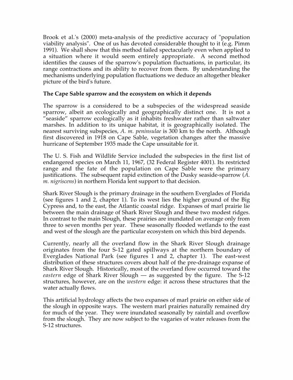
Figure 2. Three deterministic simulations of a model described in the text for thesub-population west of Shark River Slough. The proportional maximum changefrom one year to the next (R) varies from 1.61 ("wildly optimistic"; at top),through 1.34 ("optimistic", middle) to 1.24 ("plausible" bottom). The solid lineuses the known extent of available breeding habitat available for first and secondclutches over the 20 years prior to 1997. It then repeats the same pattern. Thisextent is driven by managed water flows. Were massive, dry season releasesprevented, more habitat would be available for second clutches (dashed lines).As the text discusses, only the "plausible" model is consistent with the knownpopulation estimates in 1981, 1992 and subsequent years.

0

1 0 0 0

2 0 0 0

3 0 0 0

4 0 0 0

Pop

ulat

ion

size

1 9 7 5 2 0 0 0 2 0 2 5 2 0 5 0

Year

0

1 0 0 0

2 0 0 0

3 0 0 0

4 0 0 0

Pop

ulat

ion

size

19

75

20

00

20

25

20

50

0

1 0 0 0

2 0 0 0

3 0 0 0

4 0 0 0

Pop

ulat

ion

size

97

5

20

00

20

25

20

50

R = 1.61

R = 1.34

R = 1.24

thereafter with the observed last 20-year sequence of water levels repeatedcyclically. This starting point in 1977 allows the population to increase to itsestimated value of 2500 birds by the time of the 1981 survey.

The model caps the population at 3500 birds — an estimate of carrying capacitythat doesn't strongly enter into the model's results because water levels so rarelyallow the birds to breed across the potential range. (We estimate the cap basedon the maximum available habitat and typical maximum observed densities.)

The estimates of actual range show, for example, that in 1977 all 2000 birds hadthe chance to raise one brood, but only 11% of them were in places dry enough toraise a second, even had they otherwise been able to do so.

The three scenarios of figure 2 show that only the "wildly optimistic scenario"allows the population to persist. Both optimistic scenarios fail to match twofeatures of the range-wide survey of the birds. First, the population in 1992 wasestimated to be 7% lower that it was in 1981. (There were no surveys inintermediate years and in those years there were some years when substantialareas suffered prolonged flooding.) Both optimistic scenarios suggest anincrease in numbers between 1981 and 1992. Second, these models do notrecreate the drop in population that followed the wet years of 1993 to 1995inclusive, when the population estimates fell to fewer than 400 birds. The"plausible model" predicts fewer birds in 1992 than 1981, but even it predicts~800 birds after these wet years. (So, it too is rather optimistic.)

The catastrophic years of 1983, 1984, 1986, 1987, 1993 and 1995, were not naturallybad years. They resulted from deliberate, massive dry season releases of waterthrough the S12s into Everglades National Park (Nott et al. 1998). Thecontribution of rainfall to the water levels is relatively small in comparison.

A second validation of the model and its parameters requires the sparrows topersist in the absence of these unnatural events. Were the sparrows predicted todecline, then we might suppose the model must err in not allowing the birds torecover quickly enough. A second set of models runs this "what if" alternative.If, during the catastrophic years, the sparrow's habitat had not been flooded earlyin the season and if 100% of the habitat had been available for one brood, thenthe population would have thrived under all three scenarios. Indeed, it wouldhave often reached the model's population ceiling of 3500 birds (Figure 2).

Thus calibrated, we run our model for more sets of 20 years. It re-cycles the exactpatterns of habitat availability, whereupon, the population declines towardsextinction within fifty years in the "plausible" scenario (Figure 2 c). It even goesto extinction in the "optimistic one" (Figure 2 b). What if water were notreleased? The population dips below its population ceiling periodically, butpersists indefinitely even in the plausible scenario.

We conclude that repeating managed water flows with the pattern of the last twodecades would rapidly drive this endangered species to extinction in the areathat once held the largest number of birds. The survey data we have collectedsince 1997 confirms this speculation. The population has remained under 500birds and it is restricted to a few square kilometers of habitat.

The sub-populations to the north and east of Shark River Slough (C, F)

Managed high water levels are not an issue in the other sparrow populations;indeed, it is the shortage of water that is the problem. Here, frequent fires burnthe prairies. We do not find birds in areas that are burned as often as once everytwo years (Curnutt et al. 1998). We see little point in running risk analyses ofthese populations. In total, they number a few hundred birds scattered across awide area that fires burn, in some cases, annually. Thus the birds are alreadyscarce and the threats to them are self-evident. More important is the question ofwhether fires that start in this area might spread southwards to burn the onlyarea where more than 1000 birds remain — the southeast population.

The southeastern sub-population (B)

Small portions of this area burn every year often as consequence of fires thatburn out of the pinelands to its north. Yet in 1989 nearly half of it burned as aconsequence of a massive, dry-season fire. (And probably all of sub-populationE did, perhaps explaining why it is still recovering.) Such fires can burn manyhundreds of square kilometers in the Everglades. This size dwarfs the sparrow'srange: the population in the southeast occupies only about 60 square kilometers.The policy of Everglades National Park is not to allow major fires to cross thepark roads that divide this population into three parts. Nonetheless, fires of thissize are hard to control in practice.

We model this area's population using the "plausible scenario" calibrated above.We "set" small fires (1/40th of the available habitat) every year in 20% of thathabitat. Birds within these areas cannot breed successfully that year, but do notsuffer any direct mortality. We do not know how many adult birds die in fires,but it surely more than we have assumed. In the year after fire, we assume that50% of the birds can breed in an area, 75% the year after that, and 100% thefollowing year. Curnutt et al. (1998) show that sparrow populations increase forfive or more after fires, so these estimates are also optimistic. Finally, we varythe frequency of severe fires — those that burn 90% of the bird's habitat.

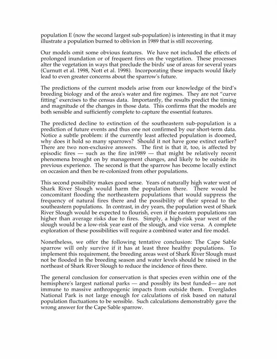
Figure 3 provides two sample simulations with severe fires every ten years andevery twenty years. In the former case the population quickly goes to extinction,in the latter case it persists. These simulations are typical. With fires on averageevery ten years, only 5% of the simulations allowed the population to increaseover a 50-year period. (That meant that the minimum population was in the firstyear of the simulation). Some 50% of the simulations resulted in the populationsdropping below 1000 birds and 15% below 500 birds (from their original start of2000). Given enough years, all the model runs encountered a bad run of firesthat drove the population to extinction.

Figure 3. Examples of stochastic simulations of a model described in the text forthe largest remaining sub-population. Twenty percent of the habitat is burnedeach year, on average, plus there are "bad" fires that burn an average of 90% of it.Such fires every 20 years allow the population to persist, those every 10 years donot.

In sum, the southeast population is in danger of extinction from extensive fires asfrequent as one in ten years. Since we have observed such fires in or near thispopulation at the frequency, we conclude that this population too is at severerisk of extinction.

Conclusions

We predict that the sparrow sub-population west of Shark River Slough willdecline to extinction if the pattern of managed flows over the S12s for the last 20years is repeated. If these unnatural breeding season flows over the S12s arestopped, this sub-population will flourish. The sub-populations in the northeasthave already declined to near extinction. These declines will continue unless thefire regimes are changed. On its own, the sub-population in the southeast runsthe risk extinction because of episodic, large-scale fires. The fate of sub-

0

1 0 0 0

2 0 0 0

3 0 0 0

4 0 0 0

Pop

ulat

ion

size

1 9 7 5 2 0 0 0 2 0 2 5 2 0 5 0

Year

Bad fires every20 years

Bad fires every 10 years

population E (now the second largest sub-population) is interesting in that it mayillustrate a population burned to oblivion in 1989 that is still recovering.

Our models omit some obvious features. We have not included the effects ofprolonged inundation or of frequent fires on the vegetation. These processesalter the vegetation in ways that preclude the birds' use of areas for several years(Curnutt et al. 1998, Nott et al. 1998). Incorporating these impacts would likelylead to even greater concerns about the sparrow's future.

The predictions of the current models arise from our knowledge of the bird’sbreeding biology and of the area's water and fire regimes. They are not “curvefitting" exercises to the census data. Importantly, the results predict the timingand magnitude of the changes in those data. This confirms that the models areboth sensible and sufficiently complete to capture the essential features.

The predicted decline to extinction of the southeastern sub-population is aprediction of future events and thus one not confirmed by our short-term data.Notice a subtle problem: if the currently least affected population is doomed,why does it hold so many sparrows? Should it not have gone extinct earlier?There are two non-exclusive answers. The first is that it, too, is affected byepisodic fires — such as the fire in1989 — that might be relatively recentphenomena brought on by management changes, and likely to be outside itsprevious experience. The second is that the sparrow has become locally extincton occasion and then be re-colonized from other populations.

This second possibility makes good sense. Years of naturally high water west ofShark River Slough would harm the population there. There would beconcomitant flooding the northeastern populations that would suppress thefrequency of natural fires there and the possibility of their spread to thesoutheastern populations. In contrast, in dry years, the population west of SharkRiver Slough would be expected to flourish, even if the eastern populations ranhigher than average risks due to fires. Simply, a high-risk year west of theslough would be a low-risk year east of the slough, and vice versa. A completeexploration of these possibilities will require a combined water and fire model.

Nonetheless, we offer the following tentative conclusion: The Cape Sablesparrow will only survive if it has at least three healthy populations. Toimplement this requirement, the breeding areas west of Shark River Slough mustnot be flooded in the breeding season and water levels should be raised in thenortheast of Shark River Slough to reduce the incidence of fires there.

The general conclusion for conservation is that species even within one of thehemisphere's largest national parks — and possibly its best funded— are notimmune to massive anthropogenic impacts from outside them. EvergladesNational Park is not large enough for calculations of risk based on naturalpopulation fluctuations to be sensible. Such calculations demonstrably gave thewrong answer for the Cape Sable sparrow.

Critics may counter that this is a special case. The species occupies a wetlandand perhaps wetlands are uniquely vulnerable to the vagaries of water flowsupstream. Perhaps; but we are not convinced. Other large parks have uniqueproblems that cross their boundaries. Fire, and our inclination to suppress smallfires and so risk catastrophic ones, is an example that comes to mind for manyparks in the western U.S.A, for example.

We argue that even for the largest protected areas we must develop mechanisticmodels of what causes populations to decline. Unless we do so, we will notpredict future risks adequately.

References

Ariño, A. and S. L. Pimm. 1995. On the nature of population extremes.Evolutionary Ecology 9:429–443.

Baillie, J. and B. Groombridge. 1996. 1996 IUCN red list of threatened animals.The IUCN Species Survival Commission, Gland, Switzerland.

Bass, O. L., Jr., and J. A. Kushlan. 1982. Status of the Cape Sable sparrow.Report T-672, South Florida Research Center, Everglades National Park,Homestead, Florida, USA.

Brok, B.W., J. L. O'Grady, A. P. Chapman, M. A. Burgman, H. R. Akçakaya andR. Frankham. Predictive accuracy of population viability analysis inconservation biology. Nature 404: 385–387.

Collar N. J, M. J. Crosby, and A. J. Stattersfield. 1994. Birds to Watch 2. BirdLifeInternational, Cambridge, UK.

Curnutt, J. L., S. L. Pimm, and B. A. Maurer. 1996. Population variability ofsparrows in space and time. Oikos 76:131–144.

Curnutt, J. L., A. L. Mayer, T. M. Brooks, L. Manne, O. L. Bass, Jr., D. M. Fleming,M. P. Nott, and S. L. Pimm. 1998. Population dynamics of theendangered Cape Sable seaside-sparrow. Animal Conservation 1:11–20.

Hanski, I. 1998. Metapopulation dynamics. Nature 396: 41–49.

Lande, R. 1993. Risks of population extinction from demographic andenvironmental stochasticity and random catastrophes. AmericanNaturalist 142: 911–927.

Lockwood, J. L., K. H. Fenn, J. L. Curnutt, D. Rosenthall, K. L. Balent, and A. L.Mayer. 1997. Life history of the endangered Cape Sable seaside-sparrow.Wilson Bulletin 109: 234-237.

Mace, G. M. 1996. Classifying threatened species: means and ends.Philosophical. Transactions of the Royal Society (London) B 344:91-97.

Maurer, B. A. 1994. Geographical population analysis: tools for the analysis ofbiodiversity. Blackwell Scientific, Oxford, UK.

Mayer, A. L., and S. L. Pimm. 1998. Integrating endangered species protectionand ecosystem management: the Cape Sable seaside-sparrow as a casestudy. Pages 53-68in G. M. Mace, A. Balmford, and J. R. Ginsberg, eds.Conservation in a changing world. Cambridge University Press,Cambridge, UK.

Nott, M. P., O. L. Bass, Jr., D. M. Fleming, S. E. Killeffer, N. Fraley, L. Manne, J. L.Curnutt, T. M. Brooks, R. Powell, and S. L. Pimm. 1998. Water levels,rapid vegetational changes, and the endangered Cape Sable seaside-sparrow. Animal Conservation 1:21–29.

National Research Council. 1992. Scientific bases for the preservation of theHawaiian crow. National Academy Press, Washington, D.C., USA.

Pimm, S. L. 1991. The Balance of Nature? Ecological issues in the conservationof species and communities. University of Chicago Press, Chicago,Illinois, USA.

Pimm, S. L., H. L. Jones, and J. M. Diamond. 1988. On the risk of extinction.American Naturalist 132:757–785.

Pimm, S. L., J. M. Diamond, T. R. Reed, G. J. Russell, and J. Verner. 1993. Timesto extinction for small populations of large birds. Proceedings of theNational Academy of Sciences (USA) 90:10871–10875.

Pimm, S. L. and A. Redfearn. 1988. The variability of animal populations.Nature 334: 613–614.

Pimm, S. L. and J. Curnutt. 1994. The management of endangered birds. Pages227–244 in C. I. Peng and C. H. Chou, eds. Biodiversity and terrestrialecosystems (Monograph Series, no. 14). Institute of Botany, AcademiaSinica, Taipei.

Saether, B-E, J. Tufto, S. Engen, K. Jerstad, O.W. Røstad, and J. E. Skåtan (2000).Population dynamical consequences of climate change for a smalltemperate songbird. Science 287: 854–856.

Chapter 3

Demography of the Cape Sable seaside sparrow withinEverglades National Park

Julie L. Lockwood1*,

Katherine H. Fenn2,

Jeffery M. Caudill1,

David Okines2,

Oron L. Bass jr.3,

Jeffery R. Duncan2,

Stuart L. Pimm4.

1 Department of Environmental Studies, Natural Sciences II, University ofCalifornia, Santa Cruz, CA 95064.

2 Department of Ecology and Evolutionary Biology, 569 Dabney Hall, Universityof Tennessee, Knoxville, TN 37996

3 South Florida Natural Resource Center, Everglades National Park, Homestead,FL 33034

4 Center for Environmental Research and Conservation, Columbia University,MC5556, 1200 Amsterdam Ave. New York, NY 10027, USA

Abstract:

The Cape Sable seaside sparrow is an endangered subspecies endemic to southFlorida’s everglades ecosystem. It exists in six spatially distinct areas (sub-populations A through F). Four of these have suffered greater than 50% declinesin breeding individuals since 1992. Because of the sparrow’s rarity and cautiousnature, demographic information has been difficult to obtain. We describe afive–year study aimed at collecting this data. We relate this information tomodern hydrological characteristics of the everglades as this varies across thespatial extent of the sparrow’s range and has been implicated in observed

subpopulation declines. Greater than 60% of adult sparrows survive from yearto year and 20% of juveniles return to their natal sites within two years offledging. We find that sparrows can produce up to four broods per breedingseason (March to August) and that female sparrows lay an average of three eggsper nest, two of which usually hatch. These characters vary from year to yearbut not spatially. The success of these nests varies from year to year andspatially. Nest success varies between sub-populations such that nests insubpopulation E are more than four times as likely to fledge young as nestswithin subpopulation A. Nest success within subpopulation B begins at 26%early in the breeding season, but drops to 9% after the onset of summer rains inearly June. Nests are built 16 to 21cm from the soil surface making themvulnerable to high water flow events. Sparrows generally remain within a one-km area centered on their breeding grounds and we have never observedimmigration between sub-populations. These demographic attributes combineto make the Cape Sable seaside sparrow extremely dependent on the hydrologyof the freshwater prairies it inhabits.

Introduction

The successful recovery of any threatened species requires a knowledge of itspopulation biology and ecological requirements (Clobert and Lebreton 1991).Describing population dynamics reduces to understanding rates of birth, death,immigration and emigration (Clobert and Lebreton 1991). Despite framing thequestions in straightforward terms, providing answers is often difficult. This isespecially true for the rare and cautious Cape Sable seaside sparrow(Ammodramus miratimus mirabilis) whose behavior and patchy distribution havehampered efforts to collect the most basic demographic information (Curnutt1996). This subspecies, endemic to south Florida, has been recognized asfederally endangered since 1967 (Curnutt 1996). In the last seven years,populations have declined by 50% or more in some areas (Curnutt et al. 1998,Nott et al. 1998). In order to institute management or restoration activities thatbenefit the Cape Sable seaside sparrow, we need to pinpoint the demographicfactors being compromised, how they are compromised, and to what degree.Below we describe a five-year study aimed at answering these questions.

The Cape Sable seaside sparrow lives within the Everglades ecosystem ofextreme south Florida (Werner and Woolfenden 1982, Kushlan and Bass 1982).This ‘river of grass’ is characterized by a slow overland flow originating at LakeOkeechobee in the north and entering Florida and Biscayne Bays in the south.The primary drainage system of the Everglades is a slough (Shark River Slough,Figure 2, chapter 1) that is flanked by expanses of marl prairie. These marlprairies are inundated with freshwater and support grasses and sedges (e.g.,Cladium jamaicense, Muhlenbergia filipes, and Schizachyrium rhizomatum) that standapproximately one meter tall. Water inundates these prairies when the sloughoverflows (Curnutt et al. 1998). Under natural conditions, these periods ofinundation occur from the onset of summer rains in early June until thebeginning of the dry–season in January (Curnutt et al. 1998). During the drymonths of February through May, Cape Sable seaside sparrows build low, cup-shaped nests in these marl prairies (Werner 1975, Werner and Woolfenden 1982).

Beginning in the early 1900s, a series of canals and spillways built within theEverglades began altering this overland flow of water. Management divertedwater from the eastern Everglades to control flooding around the growing urbanpopulation of greater Miami and to facilitate agriculture (Nott et al. 1998, Lightand Dineen 1994). The legacy of these efforts is that flows now drain into thewestern portion of Shark River Slough leaving the eastern marl prairies in a drystate far longer than under natural conditions. Conversely, the western marlprairies are flooded more often (Curnutt et al. 1998). Nott et al. (1998) provideevidence that these alterations in flow patterns (i.e. hydrology) have contributedto the observed sparrow population declines in the western marl prairies.Further, Curnutt et al. (1998) attribute the declines within extreme easternEverglades to frequent fires due to over-drying.

Our study researched how these varying hydrological conditions relate tochanges in Cape Sable seaside sparrow demography. However, the sparrow isonly one of many threatened species within the Everglades ecosystem (Mayerand Pimm 1998). The Everglades is slated for a multi-billion dollar restorationthat will take place over the next two decades (Lockwood and Fenn 2000). Thegoal is to aid wildlife recovery by reproducing historic water flows, yet stillprovide ample freshwater supplies and flood control for the local populous(Lockwood and Fenn 2000). This is a challenging task made more difficult by avague understanding of how hydrology effects sensitive species. Our resultsrepresent a first crucial step in defining how much, when, and where watershould flow into natural areas under restoration schemes.

Methods

Study areas

The sparrow's current range lies entirely within federally and state protectedlands in south Florida. Although most individuals live within EvergladesNational Park (ENP) at present, a significant segment live within Big CypressNational Preserve (Kushlan and Bass 1982). Our study is limited to those inEverglades National Park. The population is separated into six spatially distinct‘patches’ labeled sub-populations A – F (Fig. 1; see figure 2 chapter 1) by Curnuttet al. (1998). The dispersal information collected for this study addresses thespatial independence of each of these sub-populations.

Everglades National Park personnel conduct annual range-wide surveys of thesparrow (Curnutt et al. 1998, Kushlan and Bass 1982). From this information weknow that the sub-populations have not followed similar population trajectoriesover the past decade. Of the three sub-populations we will consider (A,B, and E),the western (A) subpopulation has declined the most. This subpopulation heldhalf the known population in the initial 1981 survey (Curnutt et al. 1998).Between 1992 and 1994, densities dropped by 90% and have yet to recover(Curnutt et al. 1998). Nott et al. (1998) attributed this decline to high waterevents that they assumed, given the magnitude, prevented successful nesting.

Subpopulation B has remained largely stable in numbers since 1981 (Curnutt etal. 1998). Subpopulation B now holds the vast majority of sparrows and is oftenreferred to as the population ‘core’. Subpopulation E declined in sparrownumbers by 50% between the 1981 and 1995 surveys (Curnutt et al. 1998). Thereason for the decline is unclear, however this area experienced numerous firesduring this period (Curnutt et al. 1998). Surveys conducted since 1997 havedocumented significant increases. Subpopulation E now holds 35% moreindividuals than were counted in 1981 (USFWS 1999).

The seven study plots within subpopulation B were chosen for their accessibility.Each approximately 0.5 km2, they lie along the one maintained road (Main ParkRoad) and the one un-maintained road (Old Ingraham Highway) that passthrough portions of the sparrow's range. In 1997 and 1998 we established newstudy plots within sub-populations A and E. The plot in A is approximately 0.5km2 while the plot in E is 1.5 km2. Monitoring these remote plots requireovernight stays and helicopter transport. Thus, these plots are visited half asoften as the others.

Monitoring

We capture and band adult Cape Sable seaside sparrows using mist–nets andplay–back recordings of their song (Bibby et al. 1992). Male sparrows areterritorial and respond to a tape–recording of their song by flying toward thesource (i.e. a recorder placed under the mist–net). Females will respond to tapedplay–back of songs or they can be flushed into a net. Females are caught lessfrequently than males. Adult sparrows are sexed based on behavior (e.g., onlymales will sing) or morphologically (e.g., presence of a brood patch for femalesor cloacal protuberance for males). It is possible to distinguish hatch–year (HY)and after–hatch–year (AHY) individuals based on plumage differences (e.g., HYbirds have short and differently colored flight feathers). It is not possible to ageadult birds. In 1997 we began banding nestlings on their fourth to sixth day inthe nest.

All banded individuals are given a USFWS aluminum band and three celluloidcolor bands. The unique color combination allows us to identify individualsthroughout the breeding season and in subsequent years. We begin searchingfor previously banded individuals in March, marking the territories of any re-sighted or recaptured birds with colored surveyors tape. We use re-sight–recapture information to generate a survivorship estimate for males usingthe Cormack–Jolly–Seber statistical model from the program MARK (White andBurnham 1997). We also calculate the proportion of individuals that are re-sighted or recaptured each year and compared these return rate values betweenthe sexes and ages.

Each year we search for sparrow nests from mid–March until early–June. In the1996 and 1999 seasons we continued searching for nests until August. In the twoseasons (1997, 1998) we did not continue past June, a separate radio telemetryproject worked from early–June until the following March (Dean and Morrison1998). We incorporate results from this study where appropriate.

To find nests we use behavioral cues (e.g., adults delivering food or givingdefensive calls) and random search–and–flush techniques (Bibby et al. 1992).Nests are checked every second or third day until fledging or failure. On eachnest visit, we record the number of eggs or nestlings present, the identity of theadults attending the nest, and the state of the nest itself. Each visit lasts less thana minute and neither the eggs nor nestlings are handled. Due to theaforementioned constraints on visiting plots within sub-populations A and E,occasionally the fate of nests found in these areas are unknown.

We test for differences in the number of eggs and nestlings per nest between sub-populations and years using ANOVA. If significant differences are found, weuse Fisher's protected least square difference (PLSD) to do post–hoc pair-wisecomparisons between means. The above information also estimates nestingsuccess according to Mayfield techniques (Mayfield 1975, Johnson 1979). TheMayfield technique calculates the daily survival probability of a nest by avoidingthe assumption that all nests found were actually observed through the entiretyof the nest cycle (Mayfield 1975). Because adults are banded with a uniquecombination of color bands, we also follow an individual's multiple nestingattempts.

We divide all nests found according to their date of hatching such that wecompare fecundity measures between the wet and dry seasons. Cape Sableseaside sparrows continue to nest after the onset of summer rains, howevernesting attempts are less common (see below and Werner 1975). All nests thathave a hatch date before 1 June are termed ‘early–season’ and all nests that havea hatch date after 1 June are called ‘late–season’. The 1 June cut–off is theapproximate time of year when the summer rains begin (Olmstead et al. 1980).We qualitatively compare Mayfield nest success rates between early– andlate–season nests. In addition, we compare numbers of eggs and nestlings usingStudent’s t-test.

Water flows within ENP have occasionally reached heights of 50cm aboveground level within the western marl prairies (Nott et al. 1998). In suchscenarios, the height at which sparrows place their nests off the ground becomesthe most important determinant of fecundity. If water levels attain heightsgreater than the average height of the nests, most will flood and fail (Lockwoodet al. 1997). For this reason, we measure the distance from the top of the soil tobottom of the nest structure (accuracy of ± 1cm) after the young fledge. We useStudent’s t-test and ANOVA to compare the average height of nests off theground between the early– and late–season and the sub-populationsrespectively.

We record all evidence of nest failure, including the presence of standing waterin the nest and destroyed eggs or nestlings. We record apparent predationevents as the unexplained loss of all nest contents between nest checks (Schaub etal. 1992). Calculation of predation rate is based on these records (Schaub et al.1992, Lockwood et al. 1997). Predation rate is calculated as the number ofpredation events divided by the number of nests with eggs or young present.

These rates are calculated over 10- to 14–day intervals starting each year from theday that the first nest was found.

Because Lockwood et al. (1997) present preliminary evidence of increasedpredation rates with increases in water level, we look for a similar effect here.We use hydrological information from an ENP monitoring station. This station(P46) is located approximately two km of all subpopulation B plots. The P46water levels function as the independent variable; predation rates calculated forthe seven subpopulation B plots are assigned as the dependent variable. Eachdata point represents a particular unit of time encompassing the 1996 to 1999breeding seasons.

The locations of banded, recaptured and re-sighted individuals are recorded inUniversal Transverse Mercator (UTM) Easting and Northing coordinates using aGlobal Positioning System (GPS). The accuracy of the GPS varies from one to20m. These locations allows us to calculate breeding dispersal distances (i.e. thedistance breeding individuals move from year to year) and natal dispersaldistances (i.e. the distance juveniles move from their place of birth to the nextbreeding season). We use Student's t–test to compare mean dispersal distancesbetween adult and juvenile sparrows.

Based on the above demographic parameters and their associated variability, it ispossible to create a simple model that produces worst and best case populationgrowth scenarios. Our purpose is not to produce a detailed viability model, butto understand how our results constrain the bird's recovery. First, we obtain thenumber of young produced per breeding attempt. To do this, we multiply theproportion of adults that breed by average clutch size and the daily probabilitythat the young will survive to fledging (Mayfield score). We then divide thisvalue by two such that productivity can be expressed per individual. (A nest isthe product of a pair of birds, obviously.) To obtain one–year population growth(X1) we incorporate juvenile (HYs) and adult survival (AHYs) rates in thefollowing way:

Xt+1 = (AHYs*Xt)+(HYs*individual productivity) (1)

Annual population growth is then expressed as:

Population growth = Xt+1 – Xt (2)

Results

Survival

We banded 247 adult (AHY) Cape Sable seaside sparrows between 1994 and1998. The number of AHY individuals banded ranged from 20 to 80 per year.We recaptured or re-sighted 118 of these 247 individuals at least once insubsequent years. The majority (82) were only seen once after banding. Thirty-six adults were re-sighted two or more years subsequent to original banding.One male, banded as an adult 1994, has been re-sighted every year since; making

this male a minimum of six years of age. A female, banded in 1995 as an adult, isa minimum of five years of age.

Of the 118 re-sighted adults, 93 (79%) were males. Using program MARK (Whiteand Burnham 1997) we derive a survival model for adult males. ACormack–Jolly–Seber model that assumes constant survivorship and recaptureprobability provides the best fit to our data. From this, survival rate is estimatedat 0.66 (standard error = 0.06) and the recapture rate is 0.65 (standard error =0.08). Thus, 66% of all adult males in our sampled population survive betweenyears.

This statistical model efficiently derives survivorship estimates while accountingfor the various pitfalls of using mark–recapture information (White andBurnham 1997). However, it poorly distinguishing differences in survival ratesand recapture rates when sample sizes are low or mark–recapture efforts havebeen underway for a short time. This being the state of our data, we can notcompare survival models between HY and AHY individuals, between males andfemales.

Return rates, or the proportion of individuals re-sighted or recaptured from yearto year, are poor estimators of survival rates for a variety of reasons (Begon1979). Yet, they do allow a glimpse into demographic differences betweenvarious groups of individuals within the population (i.e. HY vs. AHY, males vs.females). From 28% to 48% of AHY individuals return one year after banding;20% to 37% returned two years post–banding and only 5% returned four yearsafter banding. We have banded 213 juvenile (HY) sparrows; most in the nest.We can only calculate a return rate for HY individuals up to two yearspost–banding. Return rates for HY individuals ranges from 15% to 20%; nearlyhalf that of the equivalent return rate of AHY individuals. If we divide bandedindividuals according to gender, males and females show similar overall returnrates. Males return at a rate between 26% and 52%. Females return at a ratebetween 25% and 45%. We do not have enough banding information from thevarious sub-populations for a spatial comparison of return rates.

Fecundity

We found 252 Cape Sable seaside sparrow nests between 1996 and 1999. Tennests were found in subpopulation A, 212 in subpopulation B, and 30 insubpopulation E. Most nests (150) were early–season. We found 68 late–seasonnests and 34 could not be classified. Among the ten subpopulation A nests, onlyone (10%) was classified as a ‘late’. Of the 183 classifiable subpopulation B nests,60 were late-season (33%). Of the 26 subpopulation E nests that could beclassified, 7 were late-season (27%).

Although fecundity has several different definitions (Clobert and Lebreton 1991),there are three measures commonly calculated for birds: the number of nestsproduced in one breeding season, number of young produced per nest, andnumber of fledglings produced per egg laid. Below we describe each measurefor the Cape Sable seaside sparrow.

The first fecundity measure is the number of nests produced per breedingseason. The average length of the breeding season and the length of one nestcycle (i.e. phenology) influence this value. The earliest Cape Sable seasidesparrow nest was found on 20 March 1997. This nest had two eggs, but was lostto predation seven days later. Werner (1975) reports observing young from anest initiated in late–Febuary. The latest sparrow nest was found 10 July, 1999.This nest eventually fledged young on 26 July. Werner (1975) reports observingnests with eggs as late as 26 July and Dean and Morrison (1998) report catchingrecently fledged young as late as September. T. Dean reports a nest successfullyfledging young as late as 2 August 1998 (T. Dean pers. com.). Thus, Cape Sableseaside sparrows can nest from March until at least early August (122 to 142days).

The number of clutches produced in one breeding season depends upon howmuch time individuals devote to pair bonding, nest building, egg laying,incubation, nestling care, and fledgling care. Most of our observations concernegg laying, incubation and the nestling period. We recorded the timing of egglaying at eight nests. In each case, the females laid eggs every day until theclutch was complete. We observed four nests from initiation of the clutch tohatching. All four females incubated the nest 12d. We observed 101 nests fromhatching to fledging. The average nestling period length for these nests was9.15d (standard deviation = 2.12d). We have found 11 nests that were completebut held no eggs. These nests eventually held eggs an average of 2.72 days afterthey were found (standard deviation = 1.56d). Thus, we estimate that Cape Sableseaside sparrows require 30 to 35 days to build a nest, lay eggs, incubate, andfledge young.

The final portion of the nest cycle, the period of fledgling care, is the mostuncertain. We have never re–sighted a fledgling banded as a nestling within thesame breeding season and thus can add no new information to that described inLockwood et al. (1997) and Werner (1975). Adults may overlap broods and carefor fledglings as they are initiating a second clutch (essentially no time devotedto fledgling care) or they may care for young up to 20 days after leaving the nest(Werner 1975). This generates an estimate of 30 to 50 days required to completeone nesting cycle. Dividing this value into the 122 to 142 days during whichsparrows were observed breeding, yields a per annum clutch production of twoto four.

How many re–nesting attempts have we actually observed in one breedingseason? Of the 252 nests found in our study, 27 were known second clutches,three were known third clutches, and one was a known fourth clutch.

The second component of fecundity is the number of young produced in onebreeding attempt. Cape Sable seaside sparrows lay an average of 3.18 eggs pernest (standard deviation = 0.55, N = 126 nests). This average does not vary byyear (ANOVA F = 1.05, df = 3, P = 0.37) or across sub-populations (ANOVA F =1.04, df = 2, P = 0.36). Clutch size did not vary between early– versus late–seasonnests (Student’s t = 0.21, df = 111, P = 0.83).

Cape Sable seaside sparrows average of 2.85 nestlings per nest (standarddeviation = 0.86, N = 179 nests). This average varies according to year (ANOVAF = 5.57, df = 3, P = 0.0011). Post–hoc comparisons between years reveals that thenumber of nestlings per nest decreased in 1999. Nests held an average of 2.65nestlings (standard deviation = 0.87, N = 85 nests) in 1999, a value significantlylower than in 1997 and 1998. The number of nestlings per nest did not varyaccording to subpopulation (ANOVA F = 1.29, df = 2, P = 0.28) or between early–versus late–season nests (t = 0.38, df = 169, P = 0.71).

Finally, fecundity can be measured as a daily survival probability, oftencalculated using the Mayfield method (Mayfield 1975, Johnson 1979). Mayfieldnest success rates varied considerably from year to year. Nests found in 1998show the highest daily survival probability at 0.60. Nests found in 1999 showedthe lowest daily survival probability at 0.12. Comparing Mayfield nest successrates across space, shows that subpopulation E has the highest success rate at0.53 whereas sub-populations A has a survival probability of 0.12.Subpopulation B was the only group with enough information to divide theseprobabilities according to early– versus late–season. Early–season subpopulationB nests have a survival probability of 0.26 whereas late–season nests havesurvival probability of 0.10.

Lockwood et al. (1997) find circumstantial evidence that higher water levelsincrease the rate at which Cape Sable seaside sparrow nests are lost to predation.To test if the observed temporal variations in predation pressure are due todifferences in hydrology, we look for correlations in predation rate and waterlevels. Using all nests found within subpopulation B study plots, we calculatedpredation rates over 10– and 14–day intervals and compare them to the averagewater levels at the P46 hydrological monitoring station. Predation rates variedfrom 0 to 0.12 with an average value of 0.0342 (standard deviation = 0.04 ). Theaverage water level at the P46 hydrological station varied from 5.5cm abovemean sea level (MSL) to 53.36cm MSL with an average of 31.8cm MSL (standarddeviation = 13.48cm). When we plot predation rate within the subpopulation Bplots against water levels at the P46 station, the highest predation rates occurduring periods of high water (Fig. 2). Most of the points in the upper left cornerof Fig. 2 (i.e. those which have high predation rates and water levels) representtime periods occurring after 1 June. However, not all points in the upper leftcorner of Fig. 2 are late–season nests. High water levels, no matter when theyoccur, increase predation pressure within subpopulation B study plots.

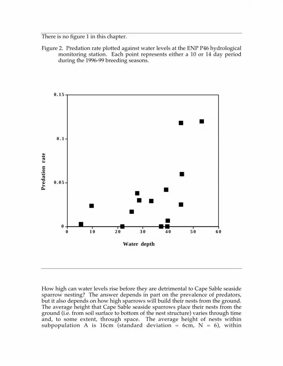
There is no figure 1 in this chapter.

Figure 2. Predation rate plotted against water levels at the ENP P46 hydrologicalmonitoring station. Each point represents either a 10 or 14 day periodduring the 1996-99 breeding seasons.

How high can water levels rise before they are detrimental to Cape Sable seasidesparrow nesting? The answer depends in part on the prevalence of predators,but it also depends on how high sparrows will build their nests from the ground.The average height that Cape Sable seaside sparrows place their nests from theground (i.e. from soil surface to bottom of the nest structure) varies through timeand, to some extent, through space. The average height of nests withinsubpopulation A is 16cm (standard deviation = 6cm, N = 6), within

0

0 .05

0 . 1

0 .15

Pre

da

tion

ra

te

0 1 0 2 0 3 0 4 0 5 0 6 0

Water depth

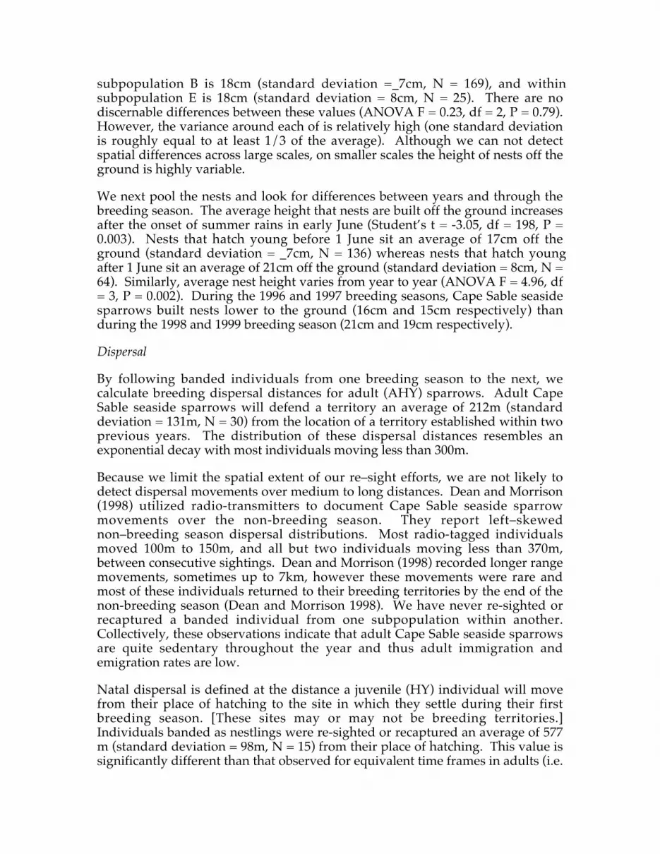
subpopulation B is 18cm (standard deviation =_7cm, N = 169), and withinsubpopulation E is 18cm (standard deviation = 8cm, N = 25). There are nodiscernable differences between these values (ANOVA F = 0.23, df = 2, P = 0.79).However, the variance around each of is relatively high (one standard deviationis roughly equal to at least 1/3 of the average). Although we can not detectspatial differences across large scales, on smaller scales the height of nests off theground is highly variable.

We next pool the nests and look for differences between years and through thebreeding season. The average height that nests are built off the ground increasesafter the onset of summer rains in early June (Student’s t = -3.05, df = 198, P =0.003). Nests that hatch young before 1 June sit an average of 17cm off theground (standard deviation = _7cm, N = 136) whereas nests that hatch youngafter 1 June sit an average of 21cm off the ground (standard deviation = 8cm, N =64). Similarly, average nest height varies from year to year (ANOVA F = 4.96, df= 3, P = 0.002). During the 1996 and 1997 breeding seasons, Cape Sable seasidesparrows built nests lower to the ground (16cm and 15cm respectively) thanduring the 1998 and 1999 breeding season (21cm and 19cm respectively).

Dispersal

By following banded individuals from one breeding season to the next, wecalculate breeding dispersal distances for adult (AHY) sparrows. Adult CapeSable seaside sparrows will defend a territory an average of 212m (standarddeviation = 131m, N = 30) from the location of a territory established within twoprevious years. The distribution of these dispersal distances resembles anexponential decay with most individuals moving less than 300m.

Because we limit the spatial extent of our re–sight efforts, we are not likely todetect dispersal movements over medium to long distances. Dean and Morrison(1998) utilized radio-transmitters to document Cape Sable seaside sparrowmovements over the non-breeding season. They report left–skewednon–breeding season dispersal distributions. Most radio-tagged individualsmoved 100m to 150m, and all but two individuals moving less than 370m,between consecutive sightings. Dean and Morrison (1998) recorded longer rangemovements, sometimes up to 7km, however these movements were rare andmost of these individuals returned to their breeding territories by the end of thenon-breeding season (Dean and Morrison 1998). We have never re-sighted orrecaptured a banded individual from one subpopulation within another.Collectively, these observations indicate that adult Cape Sable seaside sparrowsare quite sedentary throughout the year and thus adult immigration andemigration rates are low.

Natal dispersal is defined at the distance a juvenile (HY) individual will movefrom their place of hatching to the site in which they settle during their firstbreeding season. [These sites may or may not be breeding territories.]Individuals banded as nestlings were re-sighted or recaptured an average of 577m (standard deviation = 98m, N = 15) from their place of hatching. This value issignificantly different than that observed for equivalent time frames in adults (i.e.

one and two year movements; Student’s t = -4.73, df = 42, P <0.0001). In contrastto the distribution of AHY dispersal distances, HY birds move longer distancesthus producing a more even distribution of dispersal distances with a maximumnatal dispersal distance of over 1km recorded. We have not yet collected enoughinformation on HY individuals to calculate longer interval movements.

Demographic Model

We begin by exploring the best case scenario. We assume all breedingindividuals produce large clutches (3.73 = average plus one standard deviation)and these clutches have a daily survival probability equal to the maximumobserved (0.53). We will assume late breeding attempts have the same clutchsize and success rate as early attempts and that all breeding individuals thatproduced an early nest will also produce a late nest. Finally, we will assumeadults have a high survival rate of 0.72 (average plus one standard deviation)and that juveniles survive nearly as well as adults (0.50).

When we insert these variables into equation 1, we get an annual increase of70%. This is clearly very optimistic. It is unlikely that any segment of thesparrow population would ever enjoy conditions that will produce this annualrate of increase. Even under this wildly optimistic scenario, however, thesparrow population will not double in one year.

Next we change each variable to its lowest recorded value and re-calculateannual growth rate (Fig. 3.). When we change adult survivorship to its lowestrecorded level annual growth rate becomes 58%, an 8% decrease as compared tothe optimistic scenario. Changing juvenile survivorship, clutch size, or theproportion of late breeders to their lowest recorded values has similar effects,resulting in annual growth rates between 25 and 40%. The largest change ingrowth rate occurs when daily nest survival probabilities are set to levelsobserved in subpopulation A. This change, from 0.53 to 0.12 nest survivalprobability, results in a annual growth rate of –6%. Thus, even when we are veryoptimistic in all other respects, subpopulation A will decrease in numbers givenits current nest success rates.

Obviously annual growth rates will become more realistic (and less optimistic) aswe incorporate more observed demographic parameters. If our model is robust,when we insert the observed values for each subpopulation we should obtainannual growth rates that are consistent with observed population trajectories (seeabove). Subpopulation B has shown consistent numbers of individuals since thefirst population estimates were made in 1981. When we insert the demographicparameters described here into equation 1, we obtain an annual growth rate of0.23%. Subpopulation E has shown an increase in individuals since 1997 andaccordingly we obtain an annual growth rate of 27% using demographic datacollected since 1998. Subpopulation A declined by more than 90% between 1992and 1997. Since 1997 numbers have continued to slowly decline. Usingdemographic data collected since 1997, we obtain an annual growth rate of –17%.

Figure 3. Sparrow annual growth rate according to a demographic model (seetext for details). Variables are adjusted from the optimistic scenario to theirlowest value in order to ascertain their effect on annual growth rates.

Discussion

Cape Sable seaside sparrows are highly sedentary and extremely faithful toparticular breeding locations. The various sub-populations likely do not ‘trade’immigrants such that one could be the ‘source’ for another in decline (i.e., a‘sink’: Pulliam 1998). Thus, we can expect the future of the Cape Sable seasidesparrow to be played out in several smaller arenas (sub-populations), the fate ofeach determined largely independent of the others.

Cape Sable seaside sparrows are unlikely to live past three years of age and atleast 40% of the population will die each year. Juveniles are much less likely toreturn from year to year indicating that they have low first-year survivorship.These estimates are typical of small land birds (Ricklefs 1973, Perrins andBirkhead 1983) and other races of seaside sparrows (Post and Greenlaw 1994).There may be more complex survivorship dynamics within the various sub-populations, however given the nature of mark-recapture information it willrequire longer time-series to uncover them.

-20

0

2 0

4 0

6 0

8 0

An

nu

al

gro

wth

ra

te

Optimist

ic

Low a

dult

surv

ival

Low ju

v. su

rviva

l

Low c

lutc

h siz

e

Few la

te n

estin

g at

temp

ts

Low n

est

surv

ival

Cape Sable seaside sparrow fecundity reaches its maximum potential early in thebreeding season (March to June). Sparrows will continue to breed well into thewet-season, allowing this subspecies to recover from population declines.However, in order to realize this potential, most nests must be successful.Sparrows only produce two to three young per nesting attempt. If onlyearly–season nests are successful, the young produced will replace breedingadults but future population levels will remain the same. [In practice,population levels may still decline due to the low survivorship of juveniles.] Thepresence of late–season nesting is a principal means to increase sparrowdensities. Even under the best conditions we have observed (i.e. subpopulationE growing at a rate of 27% annually), it will take four years for population size todouble.

These demographic traits make the Cape Sable seaside sparrow extremelydependent on the condition of the marl prairies they inhabit. Relatively short-term excesses of water, or overly dry conditions that promote annual fires, canhave long-lasting impacts. Most resident sparrows will die within five years ofinitial impact, and if there are very few or no successful nesting attempts duringthis period, the effected subpopulation will inevitably decline. Further,managers can not rely on emigration from adjacent sub-populations to ‘rescue’the effected subpopulation.

The above discussion outlines the more subtle effects of altered hydrology onCape Sable seaside sparrow demography. However, all races of seaside sparrowincur the blunt effects of periodic high water events. Unusually high tides causemass loss of active nests in other seaside sparrow races (Marshall and Reinert1990). However, Cape Sable seaside sparrows exist within a non-tidal ecosystem.Nesting success is not influenced by tidal flooding events (Post and Greenlaw1994, Marshall and Reinert 1990). Instead hydrological influences on nestingsuccess come from annual variations in the summer rains and managementdecisions regarding water releases into Everglades National Park (Nott et al.1998).

Cape Sable seaside sparrows place their nests near the ground making themextremely vulnerable to high water events. The height of nests from the groundvaries through the breeding season, from year to year, and across small spatialscales. This variation renders inexact predictions concerning what water levelswill cause mass loss of active nests. However, we can make general predictions.The highest recorded average height of nests off the ground is 21cm (late–seasonnest average). If we add one standard deviation to this value, we can estimatethat at locations where water levels rise above 29cm during the nesting season,nearly 70% of all active Cape Sable seaside sparrow nests will flood and fail dueto inudation alone (this does not include the effects of high water on nestpredation rates). Water management decisions that reflect this fundamentalaspect of Cape Sable seaside sparrow biology will increase the probability thatthis subspecies will recover.

Predation pressure is also influenced by hydrological patterns. The higher thewater level the higher the probability that a sparrow nest will be lost to

predation. Most nest losses in our study we attribute to snakes because the neststructure is undisturbed. [The other assumed predator, the rice rat, often leavesfeces and dishevels the nests.] Some evidence implicates the cottonmouth(Agkistrodon piscivorus) in predation events. These snakes are common in ourstudy plots and T. Dean (pers. com) reports finding a cottonmouth with an adultradio–collared sparrow in its gut. If cottonmouths are the principle predators ofsparrow nests, this may explain the correlation between high water levels andpredation rate. Cottonmouths bask in the sun during the day, but are mostactive at night especially after heavy rain (Behler and King 1988).

Predation of nests is a natural event, especially for a ground–nesting species thatconstruct an open–cup nest (Martin and Li 1992, Bosque and Bosque 1995). Theimplicated predator is native to the Everglades and has likely co–evolved withthe sparrow. Thus, it is not clear what management action could be taken toreduce predation pressure beyond limiting artificial flooding during thebreeding season.

There are clear gaps in our knowledge of Cape Sable seaside sparrowdemography, such as juvenile survival and age-specific fecundity of females.However, the absence of this information should not be construed as gap in ourunderstanding of how to manage this subspecies. Our results provide clearimplications for water management, and thus define broad guidelines forrestoration of a more natural Everglades waterflow.

Acknowledgements

We thank the many individuals that helped to collect this data. We especiallyrecognize J.L. Curnutt, A.L. Mayer, R.D. Powell, K.L. Balent, R. Hirsch-Jacobson,K. Paxson, D. Rosenthal, G. Harris, G.R. Lockwood, and T. Warren. M.P. Nottgraciously offered to compute the CJS survival rates reported. Funding wasprovided to S.L.P. from the National Park Service, U.S. Fish and Wildlife Service,and the U.S. Army Corps of Engineers.

Literature Cited

Begon, M. 1979. Investigating animal abundance: capture-recapture forbiologists. University Park Press, Baltimore, M. D.Bibby, C.J., N.D.Burgess, and D. A. Hill. 1992. Bird census techniques. Academic Press,London, UK.

Behler, J.L. and F.W. King. 1988. The Audubon Society Field Guide to NorthAmerican Reptiles and Amphibians. Alfred A. Knopf, New York.

Bibby, C.J., N.D. Burgress, D.A. Hill. 1992. Bird census techniques. AcademicPress, New York, NY.

Bosque, C. and M.T. Bosque 1995. Nest predation as a selective factor in theevolution of developmental rates in altricial birds. American naturalists145:234-260.Bourliere, F. 1991. Forward. In: Bird population studies(Perrins, C.M., J.–D. Lebreton, and G.J.M. Hirons, eds). Oxford UniversityPress, Oxford, UK.

Clobert, J. and J.-D. Lebreton. 1991. Estimation of demographic parameters inbird populations. In: Bird population studies (Perrins, C.M., J.–D.Lebreton, and G.J.M. Hirons, eds). Oxford University Press, Oxford, UK.

Curnutt, J. L. 1996. Cape Sable seaside sparrow. In Rare and endangered faunaof Florida. Birds. (Rogers, J.A. Jr., H.W. Kale III, T.H. Smith, eds).University of Florida Press, Gainesville, FL.

Curnutt, J.L., A.L. Mayer, T.M. Brooks, L. Manne, O.L. Bass Jr., D.M. Fleming,M.P. Nott, and S.L. Pimm. 1998. Population dynamics of the endangeredCape Sable seaside–sparrow. Animal Conservation 1:11-21.

Dean, T. F. and J.L. Morrison. 1998. Non-breeding season ecology of the CapeSable seaside sparrow (Ammodramus maritimus mirabilis). 1997-1998 fieldseason final report. Everglades National Park, Homestead, FL.

Johnson, D. 1979. Estimating nest success: the Mayfield method and analternative. Auk 96:651-661.

Kushlan, J.A. and O.L. Bass Jr. 1983. Habitat use and the distribution of the CapeSable sparrow. In: The seaside sparrow, its biology and management.(Quay, T.L., J.B. Funderburd Jr., D. Lee, E.F. Potter, and C.S. Robbins, eds).North Carolina Biological Survey and North Carolina State Museum.

Light S.S. and J.W. Dineen. 1994. Water control in the Everglades: A historicalperspective. Pages 47 - 84 in S.M. Davis and J.C. Ogden, eds. Everglades:The ecosystem and its restoration. St. Lucie Press, Boca Raton, FL.

Lockwood, J.L., K. H. Fenn, J.L. Curnutt, D. Rosenthal, K.L. Balent, and A.L.Mayer. 1997. Life history of the endangered Cape Sable seaside sparrow.Wilson Bulletin 109:720-731.

Lockwood, J.L. and K.H. Fenn. 2000. The recovery of the Cape Sable seasidesparrow through restoration of the everglades ecosystem. EndangeredSpecies UPDATE 17(1):10-14.

Marshall , R.M. and S.E. Rheinhart. 1990. Breeding ecology of seaside sparrowsin a Massachusetts salt marsh. Wilson Bulletin 102(3):501-513.

Martin, T.E. and P. Li. 1992. Life history open- vs. cavity-nesting birds. Ecology73:579-592.

Mayer, A.L. and S.L. Pimm 1998. Integrating endangered species protection andecosystem management: the Cape Sable seaside sparrow as a case study.Pages 53-68 in G.M. Mace, A. Balmford, and J.R. Ginsberg eds.Conservation in a changing world. Cambridge University Press,Cambridge, UK.

Mayfield, H. 1975. Suggestions for calculating nest success. Wilson Bulletin87:456-466.

Nott, M.P., O.L. Bass Jr., D.M. Fleming, S.E. Killefer, N. Fraley, L. Manne, J.L.Curnutt, T.M. Brooks, R. Powell, and S.L. Pimm. 1998. Water levels,rapid vegetational change, and the endangered Cape Sable seaside-sparrow. Animal Conservation 1:23-32.

Olmstead, I.C., Loope, L.L., and Rintz, R.E. 1980. A survey and baseline analysisof aspects of the vegetation of Taylor Slough, Everglades National Park.South Florida Research Center Technical Report, T-586, EvergladesNational Park, Homestead FL.

Perrins, C.M. and T. R. Birkhead 1983. Avian Ecology. New York. Chapmanand Hall.

Post, W. and J.S. Greenlaw. 1994. Seaside Sparrow. In The birds of NorthAmerica. No. 127. (Poole, A. and F. Gill, eds). American OrnithologistsUnion, The Academy of Natural Sciences, Philadelphia, PA.

Ricklefs, R.E. 1973. Fecundity, mortality, and avian demography. In Breedingbiology of birds (D.S. Farner, ed). Washington D.C. Nation. Academy ofSciences

Schaub, R., R. Mumme, and G. Woolfenden. 1992. Predation on the eggs andnestlings of Florida Scrub Jays. Auk 109:585-593.

Sullivan, K.A. 1989. Predation and starvation: age specific mortality in juvenilejuncos. Journal of Animal Ecology 58:275-286.

Werner, H. 1975. The biology of the Cape Sable seaside sparrow. Report to USFish and Wildlife Service. Everglades National Park, Homestead, FL.

Werner, H. and G.E. Woolfenden. 1983. The Cape Sable seaside sparrow: itshabitat, habits and history. In: The seaside sparrow, its biology andmanagement. (Quay, T.L., J.B. Funderburd Jr., D. Lee, E.F. Potter, and C.S.Robbins, eds). North Carolina Biological Survey and North Carolina StateMuseum.

White, G.C. and K.P. Burnham. 1997. Program MARK: Survival estimation fromp o p u l a t i o n s o f m a r k e d a n i m a l s .http://www.cnr.colostate.edu/~gwhite/mark/euring/pdf (24 August,1999).

Chapter 4

Demonstrating the destruction of the habitat of the CapeSable seaside sparrow

Clinton N. Jenkins (1)

Robert Powell (1)

Oron L. Bass Jr. (2)

Stuart L. Pimm (3)

(1) Department of Ecology and Evolutionary Biology, University of Tennessee,Dabney Hall, Knoxville, Tennessee 37996

(2) South Florida Natural Resources Center, Everglades National Park,Homestead, FL 33034, USA.

(3.) Center for Environmental Research and Conservation, Columbia University,MC5556, 1200 Amsterdam Ave. New York, NY 10027, USA

Introduction

Countries differ in the vigor to which they protect biodiversity and in theparticular laws they pass to do so. In the United States of America, one of themost effective laws is the Endangered Species Act. It prohibits direct take — thekilling or harming — of Federally-listed endangered species. From its inceptionthere has also been the implication that it prohibits take indirectly — through thedestruction of the ecosystems on which species depend. That provision waschallenged in a legal case, Sweet Home versus Babbitt, argued in front of theSupreme Court of the United States, on February 17th 1995. In the particularcontext of the Spotted Owl, an Oregon group challenged the responsible cabinetmember, Secretary of the Interior Babbitt, arguing that only direct take violated

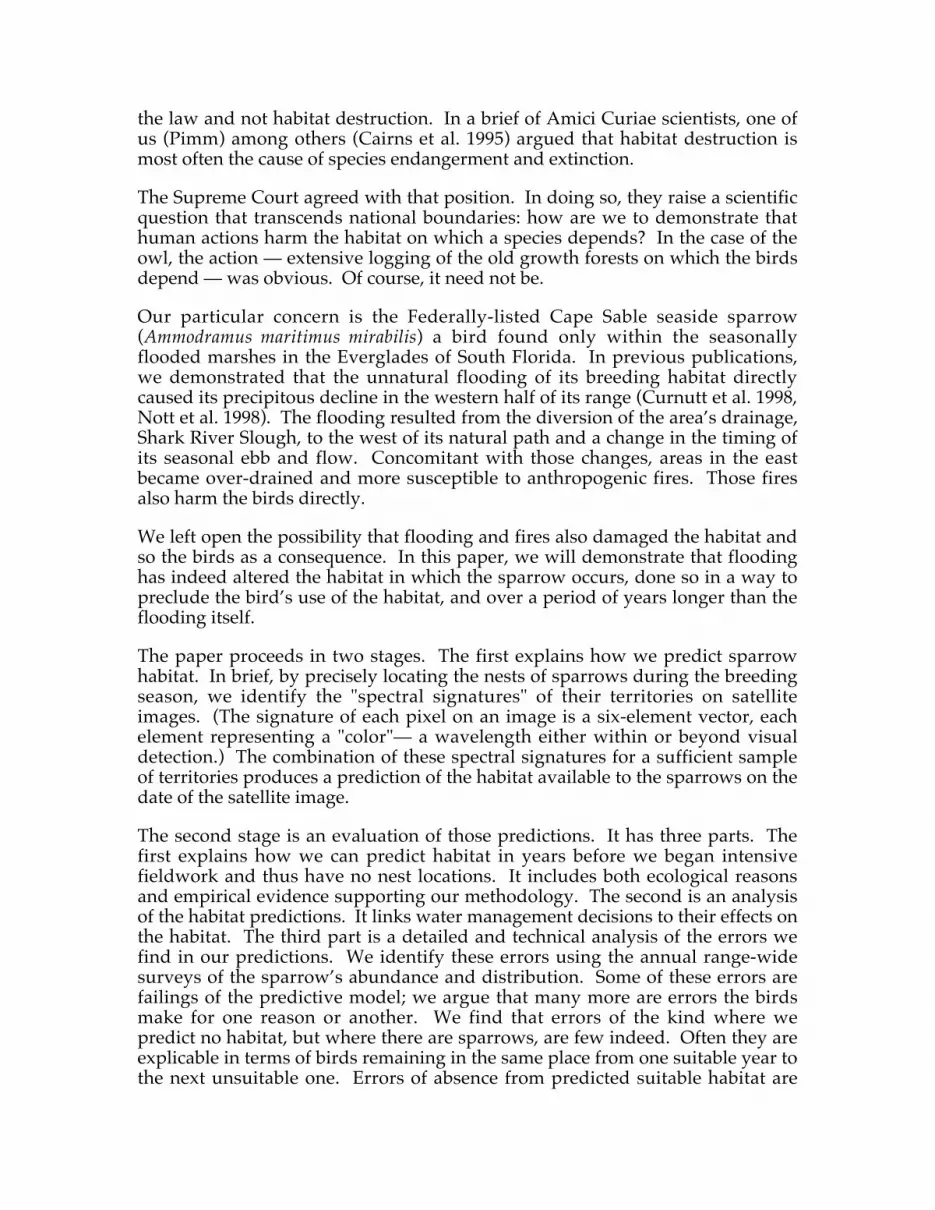
the law and not habitat destruction. In a brief of Amici Curiae scientists, one ofus (Pimm) among others (Cairns et al. 1995) argued that habitat destruction ismost often the cause of species endangerment and extinction.

The Supreme Court agreed with that position. In doing so, they raise a scientificquestion that transcends national boundaries: how are we to demonstrate thathuman actions harm the habitat on which a species depends? In the case of theowl, the action — extensive logging of the old growth forests on which the birdsdepend — was obvious. Of course, it need not be.

Our particular concern is the Federally-listed Cape Sable seaside sparrow(Ammodramus maritimus mirabilis) a bird found only within the seasonallyflooded marshes in the Everglades of South Florida. In previous publications,we demonstrated that the unnatural flooding of its breeding habitat directlycaused its precipitous decline in the western half of its range (Curnutt et al. 1998,Nott et al. 1998). The flooding resulted from the diversion of the area’s drainage,Shark River Slough, to the west of its natural path and a change in the timing ofits seasonal ebb and flow. Concomitant with those changes, areas in the eastbecame over-drained and more susceptible to anthropogenic fires. Those firesalso harm the birds directly.

We left open the possibility that flooding and fires also damaged the habitat andso the birds as a consequence. In this paper, we will demonstrate that floodinghas indeed altered the habitat in which the sparrow occurs, done so in a way topreclude the bird’s use of the habitat, and over a period of years longer than theflooding itself.

The paper proceeds in two stages. The first explains how we predict sparrowhabitat. In brief, by precisely locating the nests of sparrows during the breedingseason, we identify the "spectral signatures" of their territories on satelliteimages. (The signature of each pixel on an image is a six-element vector, eachelement representing a "color"— a wavelength either within or beyond visualdetection.) The combination of these spectral signatures for a sufficient sampleof territories produces a prediction of the habitat available to the sparrows on thedate of the satellite image.

The second stage is an evaluation of those predictions. It has three parts. Thefirst explains how we can predict habitat in years before we began intensivefieldwork and thus have no nest locations. It includes both ecological reasonsand empirical evidence supporting our methodology. The second is an analysisof the habitat predictions. It links water management decisions to their effects onthe habitat. The third part is a detailed and technical analysis of the errors wefind in our predictions. We identify these errors using the annual range-widesurveys of the sparrow’s abundance and distribution. Some of these errors arefailings of the predictive model; we argue that many more are errors the birdsmake for one reason or another. We find that errors of the kind where wepredict no habitat, but where there are sparrows, are few indeed. Often they areexplicable in terms of birds remaining in the same place from one suitable year tothe next unsuitable one. Errors of absence from predicted suitable habitat are

more common. They are most readily explainable by the bird’s inability to re-colonize once-suitable habitat that in immediately preceding years becameunsuitable because of fires or floods.

We will present two key results.

(1) Across the eight years of the study, large year-to-year fluctuations inpredicted habitat confirm the culpability of water managers. Flooding in 1993and 1995 greatly reduced the habitat predicted to be suitable for the sparrowcompared to 1992. This is a formal, technical demonstration of the figurespresented in Nott et al. 1998, inferring dry prairies in 1992 and extensivelyflooded prairies in 1993 and 1995, from the colors of the published images.

(2) The predicted suitable habitat west of Shark River Slough was at a low ebb in1995 and has recovered slowly, but consistently, in the years from then until1999. This formal, technical demonstration matches exactly the subjectiveopinion expressed by Bass and Pimm from their visual surveys. By 1999, thepredicted suitable habitat had not yet recovered to its pre-flood state. Thehabitat is recovering faster than the slowly recovering bird populations. It is therepetition of precisely such a scenario that we predict could lead to the species’extinction (Pimm and Bass 2000).

Neither of these results are surprises, for they were suggested by our previouspapers. Nonetheless, we consider the details present here to be important inboth a national and a broader context. Importantly, our data conclude that watermanagement practices have damaged huge areas of vegetation across EvergladesNational Park, have done so for extensive periods of time, and in a way thatjeopardizes the survival of a Federally listed species. This constitutes a "take."Moreover, it is one that is independent of, and lasts longer than, the direct affectsof flooding. Crucially, these data are independent of — and so additional to —all other conclusions that we have drawn in previous papers.

More broadly, we have used satellite imagery to predict potential habitat, itsfluctuation from year to year, and calibrated these changes against known birdnumbers. This is a singular result with few, if any, precedents.

Figure 1 – Location of sparrow populations (A-F) in Everglades National Park.Water enters the park from two sources, the S-12 floodgates and a pumpingstation north of Taylor Slough. The S-12 floodgates are west of the natural entrypoint for water into the ecosystem. (The natural flow path is illuminated by thetree islands, which line up with it. They appear as pale, tear-drop shaped objectsamid the darker, flooded areas of the Slough.) Whenever the S12s open theyflood population A. Additionally, shifting of water to the west causespopulation F to become drier and to suffer an increased fire frequency. Thepumping station north of Taylor Slough affects the water levels in populations Cand D. Heavy pumping results in the complete flooding of D and thesoutheastern portion of C. Populations B and E are less affected by flooding.

The Cape Sable sparrow, its habitat, and its history

The approximately 2000 pairs of Cape Sable sparrows live entirely within 1500km2 of Florida’s Everglades. The birds live in six populations separated tovarious degrees by the area’s main drainage, Shark Slough, and areas ofunsuitable (typically wood or bushy) habitat (Figure 1).

Bass and Kushlan (1982) conducted the first extensive sparrow survey in 1981.We repeated the survey in 1992 and annually thereafter. Across a 1 km by 1 kmgrid of more than 600 sites, we record the number of sparrows seen or heardwithin a 7-minute interval. We take particular care to visit all locations thatmight hold sparrows and do not observe birds at most of the sites we survey.This suggests that we do not miss many (if any) sites that hold birds.

To estimate the actual numbers of sparrows from the number we observed onour survey, we multiply each singing male by 16. This correction is based on therange at which we can detect the sparrow’s distinctive song — it encompasses1/8th of a square kilometer, roughly a circle with a diameter of 200 meters — andon the assumption that one female accompanies each singing male; Curnutt et al.(1998) provide details.

Using this calibration, we estimated that the total breeding population of thisspecies was over 6000 in both 1981 and 1992. Of the six populations, A (west ofShark River Slough) was the most numerous in 1981 (~2700 birds) and B heldfewer birds (~2300). Population B held more than A in 1992 (~3000 versus ~2600). Population E consistently held ~600 birds. The other three populationsheld between 100 and 400 birds, although we found no birds in F in 1992.

Table 1 lists the numbers of survey points and birds heard during each yearlysurvey. The number of survey points ranges from between 478 and 853. Table 1lists from 416 to 721 because we exclude some outlying areas that hold few, ifany birds. (These include Cape Sable itself where the bird was first collected andwhere habitat changes have subsequently made the location unsuitable for it.)Some of the earlier surveys deliberately explored areas thought unlikely to holdbirds to confirm that they did not. In 1992, for instance, the survey extendedacross much of the deep-water areas of Shark River Slough. Recent surveysattempt to count at every location that has held birds in the past or that we thinkthat is even remotely potential habitat. For quantitative habitat comparisons, wedemarcate populations by drawing a polygon around all survey points that everhave birds or were in any of the 1997 through 1999 surveys (Figure 1).

Populations A and B were the two largest populations in 1981 and 1992 andconsequently have most of the survey points (table 1). In 1994, the survey wasincomplete because of mechanical difficulties. Populations C, D, and F have nosurvey results and E is incomplete. The 1996 survey was incomplete forpopulation F.

Table 1. Number of birds heard (top) in number of survey points (bottom) ineach population in each year. ‘NS’ means there was no survey and ‘inc’ meansthe survey was incomplete.

Birds heard

Population 1981 1992 1993 1994 1995 1996 1997 1998 1999

A 156 146 24 5 14 24 17 11 25

B 147 199 154 135 130 118 177 113 128

C 27 3 0 NS 0 3 3 5 9

D 25 7 6 NS 0 5 3 3 11

E 42 37 20 7/inc 22 13 52 57 48

F 7 0/inc 0 NS 0 1/inc 1 1 1

Total 404 392 204 147 166 164 253 190 222

Points surveyed

A 338 347 338 284 340 167 228 263 297

B 137 146 149 132 159 130 135 136 133

C 40 41 40 NS 40 38 34 40 39

D 67 67 67 NS 67 56 46 50 50

E 73 79 75 16/inc 74 63 66 77 88

F 41 3/inc 41 NS 41 11/inc 35 32 36

Total 696 683 710 416 721 465 544 598 643

Although populations A and B were of similar size in 1981 and 1992, floodsduring the breeding seasons of 1993, 1994, and 1995 prevented the birds fromnesting across much of population A. Sparrows nest close to the ground andnestlings drown or suffer increased predation during floods (Lockwood et al.1997). Like other small-bodied passerines, the expected lifetime is about oneyear, so only a few old birds survived to see the drier conditions of 1996.

Population B remained relatively constant throughout the study period.Populations C and D had moderate numbers of birds in 1981, but during thisstudy period consistently have few birds.

Population E had two sub-populations in 1992. We speculate that this was theresult of the very large fire in 1989. Much of the middle and southern portions ofthe population burned, but part of the northern portion was undamaged. Birdsin the northern sub-population were present in every year of the survey.However, in 1995 opening of the S-12 floodgates flooded part of this sub-population and there was an associated decline in numbers. Since 1996, thenorthern sub-population has been increasing and expanding southward. Thesouthern sub-population held a substantial number of birds in 1992, but sincethen has faired poorly due to flooding. Survey records indicate that the area hadmore sawgrass (Cladium jamaicensis) in 1992 than is typical of sparrow habitat,suggesting a wet history. However, from 1989 to 1992, which were very dryyears, all of this area was dry. It may be that this typically wet area becamesuitable for sparrows with the dry conditions and they expanded into it. Then, in1993 and many subsequent years, the area floods and the birds disappear. Since1993, birds occur only sporadically.

Population F is always small, likely because the area suffers frequent fires.

Floods and fires directly harm the birds and their nests. The question we askhere is whether they have also harmed the habitat on which the birds depend. Ifso, a second question follows: how quickly does the habitat recover? Clearly, thebirds cannot recover until their habitat does.

Stage I: Predicting the habitat

To produce a map of a species’ habitat using satellite imagery, we need toincorporate all the features of a species’ natural history that are identifiable onthe image. For the sparrow, our field experiences suggest a minimum of threefeatures: vegetative structure, proximity to bushes, and patch size.

Our first stage is to identify what spectral responses correspond to suitablesparrow habitat. Different vegetative structures give different spectral responsesor signatures. Even in the gray-scale image in figure 1, it is possible to tell thedifference between the wetter vegetation in the central part of Shark RiverSlough and the drier prairies on either side. In color (see Curnutt et al. 1998) andat a finer resolution, it is possible to pick out many other more subtle vegetativefeatures.

We locate over 200 nests using a Global Positioning System (GPS) and thenmatch each of these nests to their corresponding pixel on the satellite images.The resolution of these images — the pixel size — is 29 by 29 meters. These pixelsform the basis of the prediction of potential sparrow habitat.

The second stage involves the proximity to bushes. Predators, such as Red-shouldered Hawks (Buteo lineatus), perch on bushes and shrubs when looking forprey, such as the sparrow. Nesting close to bushes likely exposes sparrows to anincreased risk of predation. So we ask: how close to bushes do the birds nest?After answering that question, we eliminate areas that are too close.

In the third stage, we eliminate patches that are too small to hold a breedingterritory.

In brief, to predict sparrows present, an area must contain a sufficient number ofpixels with the correct spectral signatures to enable a sparrow to establish aterritory and these pixels must not too close to bushes. We now present thesesteps with the requisite details.

Predicting habitat 1: Obtaining the spectral signatures

This stage has three parts. First, we correct the satellite images so our GPS datawill match up correctly with the image. Second, we make spectral signatures ofsuitable sparrow habitat using the nest pixels. Last, we apply these spectralsignatures to the image to map the habitat.

Images and rectification. We use Landsat Thematic Mapper (TM) images takenduring the breeding seasons of 1992 through 1999. When possible, these arefrom April or May, the months of the peak breeding season. In 1996, no cloudfree image was available in April or May and we used one from March 21. In1997, all images in the breeding season were cloudy.

Landsat TM images consist of seven spectral bands ranging from blue (0.45-0.52µm) to thermal (10.4–12.5 µm). Using the thermal band reduces the accuracy ofour results because the prairie is essentially at thermal equilibrium. Weeliminate it from our analyses.

We took coordinates for 66 ground control points using a differentially correctedGPS (< 2 m error) in accessible areas and from quadrangle maps (1:24000) ininaccessible areas. We use these to correct for misalignments and distortions inthe satellite images. This process, known as rectification, smoothly stretches theimage to produce a least square fit to the control points. The difference betweenthe predicted positions of the control points and their true values had a rootmean square error of 2.9 meters, that is, 10% of the linear dimension of eachpixel.

Making spectral signatures. Using the differentially corrected GPS, we tookcoordinates for 261 nests from 1996 through 1999. We eliminate nest locationsjudged to be of questionable accuracy and those closer than one pixel (29m) to aroad. Presence of a road within a nest pixel contaminates the spectral signature.This leaves 232 usable nests. For each year, we discard nest locations if they fallon clouds, shadows, or other features corrupting the image.

Using only the nest pixel provides no information on the spectral characteristicsof the surrounding habitat within the territory. Sparrows defend territories ofabout 2 hectares (Werner et al. 1974, our unpublished data). In an ideal world,we would have precise maps of sparrow territories and build our spectralsignatures from those. However, in most cases we have only the nest locationand must work from that. Therefore, we need to select pixels that adequatelyrepresent the true territory. To select those pixels we tried two methods.

The central place foraging method assumes that sparrows place their nest in thecenter of their territory. This would minimize the distance flown to feednestlings and the distance to defend territory boundaries. We use the 25 nearestcontiguous pixels (2.1 ha) that are not obviously unsuitable (i.e., bushes orwater). (25 produces a compact, if not quite circular pattern, with the nestlocation centrally located.)

The minimum spectral distance method assumes that sparrows place their nest in atypical part of the territory. We then select the 25 contiguous pixels that are mostsimilar to the nest pixel. That is, they have the minimum spectral distance fromthe nest pixel.

Our field experience, including mapped territories that were irregular in shapeand had nests near their boundaries, suggested that this second method shouldbe the better one. Indeed, our results support this. In direct comparisons of thefirst and second methods, the latter classifies more habitat in areas with birdsand less habitat where there are none. In what follows, we only use theminimum spectral distance method.

Making and summing classifications. For a particular nest and its associated 25pixels, we calculate the minimum and maximum value within each of the sixspectral bands. This produces a six-dimensional box within which we deem allenclosed pixels to be predicted habitat. This is one sparrow’s opinion of suitablehabitat. Clearly, we can do this for all the available nests and territories andcombine those opinions.

We can combine those opinions in a large variety of ways. Samples based on fewnests will likely perform less well than those based on large samples. Moreover,in some years we have no nests at all. To get the largest samples we couldcombine nests from different years. This runs the risk of combining years wherethe birds placed their nests in different places because of different waterconditions, for instance. To resolve these difficulties, we need to compare andcontrast the predictions they produce. This we will do, but first we must explainthe final two stages.

Predicting habitat 2: The bush layer

We find that sparrows do not nest near bushes, presumably because of increasedpredation risk. Using aerial photography, we measured the distance of 52 nestsfrom the nearest bush. Figure 2 shows a sharp increase in nest frequency after40m from a bush. Therefore, we eliminate classified habitat within 2 pixels (~58

m) of a bush.

Bushes are high in chlorophyll — they are green — compared to the buff tones ofthe prairie grasses. The satellite images capture these visually obvious features,particularly the cloud-free image from 1994 image. Because of the large spectraldifferences between bushes and other prairie vegetation, we use the ISODATA(Jensen 1996) algorithm to automatically find signatures corresponding tobushes. Accuracy assessment with aerial photography shows that this algorithmcorrectly identified pixels containing bushes >5-meters is diameter or clusters ofsmaller bushes.

Figure 2 – Distance between nests and nearest bush. Few birds nest with 60meters of a bush.

Predicting habitat 3: eliminating small habitat patches

Because sparrows need enough suitable habitat for a breeding territory, weeliminate patches of habitat smaller than 25 pixels (2 ha) from the predicted areaof habitat. We use 25 pixels to be consistent with the territory size used inmaking signatures.

How close will sparrows nest to bushes

02468

1012

0-20 20-40

40-60

60-80

80-100

100-120

120-140

140-160

160-180

180-200

Distance from bush (m)

Fre

qu

ency

Stage II: Evaluating the predictions

The evaluation stage has three parts. Any attempt at prediction begs twoquestions: "of what?" and "by what?" The first answer is simple — birddistributions. It is the second that is more subtle. Certainly, we could predictdistributions of birds in each population in each year from nest locations in eachpopulation and in each year. But prediction usually seeks efficiency. Ours is theability to predict distributions in all populations in all years from a sample ofnests that will be from only the more accessible populations and only from someof the years. The first stage explores how accurately we can do this.

The second stage is an analysis of the habitat predictions within each of thepopulations. It links water management decisions to their effects on the habitatand the population.

The third part is a detailed and technical analysis of the errors in our predictions.We defer this to Appendix 1.

Each of these components uses the annual range-wide surveys of the sparrow’sabundance and distribution. Tests in the intensive study areas indicate anobserver can hear a singing sparrow up to 200 meters away — an area of about13 hectares. We calculate how much predicted suitable habitat is within a circleof 200-meter radius about the survey point. If the model predictions are good,then the survey should find birds more often in areas where the model predictsmore habitat. In a graph of sparrow presence versus amount of habitat predicted(Figure 3a) the curve should be low on the left side (less habitat predicted) andhigh on the right side (more habitat predicted).

Predicting habitat in years without enough nests

We only have nest locations from 1996 onward, and 1996 and 1997 have too fewnests for good results. However, we need to predict habitat from 1992 onwards.An efficient solution would be to use nests from all available years on every year’simagery. This provides a large sample size and allows predictions in every year.Both ecological and empirical evidence support this approach.

The ecological evidence is the consistency of habitat within our study sites. Theyare primarily in areas that have not flooded or burned since 1992. A criterion fororiginally selecting these locations was that they had a consistent sparrowpopulation and thus suitable habitat. Therefore, we posit that the areas in whichsparrows nested during the detailed surveys, 1996 through 1999, were alsosuitable habitat in prior years. Sparrows nest in very similar places each year, sothat a nest in 199x would almost certainly be within a territory in 199y.

Figure 3 (b) through (d) shows the empirical results supporting our assumption.These graphs compare nests from 1998, 1999, and from all years on various years’imagery. (We have too few nest locations in 1996 and 1997 to separate them out.)

Ideally, we would get a graph comparable to figure 3a, showing a monotonicrelationship between habitat predicted and probability of finding birds. Belowsome threshold amount of habitat (the vertical line) there would be insufficienthabitat to hold birds. Should we find birds in such areas we would have anomission error. (Our model errs in omitting places where the birds occur.) Abovethis threshold, we should find birds and, were we not to do so, we would have acommission error. Ideally, both omission and commission errors would be small,when there would need to be a sharp transition about the threshold. In reality,the graphs are more variable, but the relationship still holds.

Figure 3 – The proportion of sites surveyed by helicopter where one or morebirds were encountered versus the percentage of the area predicted to containsuitable sparrow habitat on the basis of different sets of nests. (a) Ideally, as themodel predicts more habitat the survey will find more birds, thus we should seea positive slope. (b-d) In reality, the results have noticeable variability, but doshow a definite positive slope. Each line corresponds to a combination of nests(1998, 1999, or all) used as seed pixels and years of imagery analyzed (nest yearor non-nest year). All years is a summation of the results from every year’simagery using a given set of nests.

1998

0.00

0.10

0.20

0.30

0.40

0.50

0.60

0.70

0 1-9% 10-19% 20-2 9% 3 0-39% 4 0-49% 50-5 9% 6 0-69% 7 0-79% 80-8 9% >89%

% o f a rea c las s if ied a s hab ita t

1998 nests - 1998 image

1998 nests - non 1998images

all nests - 1998 image

b

1999

0.00

0.10

0.20

0.30

0.40

0.50

0.60

0.70

0 1-9% 10-19% 20-2 9% 3 0-39% 4 0-49% 50-5 9% 6 0-69% 7 0-79% 80-8 9% >89%

% o f a rea c las s if ied a s hab ita t

1999 nests - 1999 image

1999 nests - non 1999images

all nests - 1999 image

c all years

0.00

0.10

0.20

0.30

0.40

0.50

0.60

0.70

0 1-9% 10-19% 20-2 9% 3 0-39% 40-49% 5 0-59% 60-6 9% 7 0-79% 80-8 9% >8 9%

% o f a re a c la ss ified a s habita t

1998 nests - all years

1999 nests - all years

all nests - all years

d

In figure 3b, using 1998 nests to predict where birds should be encountered on1998 imagery gives a strong, but variable, increase in the proportion of surveypoints containing birds as the amount of predicted habitat increases, as weexpect. When using 1998 nests on non-1998 images a similar pattern occurs.Thus, 1998 nests predict habitat just as well in other years as they do their own.In figure 3c, using 1999 nests on the 1999 image and other years gives a similarresult. Thus, 1999 nests work as well. For both 1998 and 1999 images, using allnests produces the same pattern. Figure 3d shows a summation of results fromusing 1998, 1999, and all nests to map sparrow habitat. Again, none of the curvesdiffers substantially from each other. These results indicate that the year of thenest does alter the efficacy of the predictions. Likely, nest locations areconsistently good habitat, at least within the time span of this study.

We conclude that nests from one year are usable for predicting habitat in otheryears. To gain the maximum sample size we use all nests to map habitat in eachyear. This provides the opinions of the most sparrows' and thus predicts themost habitat.

Habitat analysis

To estimate the total potential habitat, we combine habitat classifications for allyears. Looking at the six populations together, we estimate 459 km2 heldpotential habitat in one or more years. Among the populations, A and B have themost potential habitat with 138 km2 (30% of the total) and 116 km2 (25%)respectively. Population E is third with 82 km2 (18%), and C, D, and F have 31km2 (7%), 54 km2 (12%) and 38 km2 (8%) respectively.

Not all these areas will be suitable habitat each year. In any given year, floods,fires, and other environmental factors reduce the potential habitat, leaving asubset that is currently suitable. Looking at the average amount of this suitablehabitat reveals a different pattern than looking at only potential habitat. Overall,the habitat suitable for the birds each year averages 240 km2 (52%). Population Aaverages only 38 km2 (28%) of its potential, reflecting the large amount of habitatdestroyed by floods in 1993 and 1995 and the slow recovery thereafter.Population D, also affected by flooding, averages just 20 km2 (37%). PopulationsB and E are relatively constant and have the highest average amount of habitatwith 85 km2 (73%) and 54 (66%) respectively. Populations C and F average 19km2 (61%) and 23 km2 (61%) respectively.

How much of this suitable habitat do the birds occupy?

An important pattern emerges from figure 4. Populations with large year-to-yearfluctuations in habitat support fewer birds. After a flood or fire reduces thehabitat and then the habitat recovers, it takes time for sparrows to disperse andfully occupy it. Consequently, the more variable the habitat, the less efficientlysparrows are able to occupy it.

Figure 4 – Area (km2) occupied by sparrows (columns) and area of suitablehabitat (lines). We calculate the occupied area by multiplying the number ofbirds counted in the survey (table 1) by 8 to estimate the total number ofbreeding territories, equivalent to breeding males. Each territory is 2 ha or .02km2. The y-axis is a logarithmic scale. ‘NS’ means there was no survey and‘INC’ means the survey was incomplete.

Figure 4 shows these predicted amounts of suitable habitat and their variationfrom year to year. It also shows the estimates of the area occupied by sparrows.To calculate these numbers, we take the number of birds heard on the survey in

A

0.1

1.0

10.0

100.0

1992 1993 1994 1995 1996 1998 1999

are

a o

f h

ab

ita

t (k

m2)

B

0.1

1.0

10.0

100.0

1992 1993 1994 1995 1996 1998 1999

are

a o

f h

ab

ita

t (k

m2)

C

0.1

1.0

10.0

100.0

1992 1993 1994 1995 1996 1998 1999

are

a o

f h

ab

ita

t (k

m2)

D

0.1

1.0

10.0

100.0

1992 1993 1994 1995 1996 1998 1999

are

a o

f h

ab

ita

t (k

m2)

E

0.1

1.0

10.0

100.0

1992 1993 1994 1995 1996 1998 1999

are

a o

f h

ab

ita

t (k

m2)

F

0.1

1.0

10.0

100.0

1992 1993 1994 1995 1996 1998 1999

are

a o

f h

ab

ita

t (k

m2)

each population (table 1), multiply by eight territories (for the survey counts onlyone territory in eight — see above) and then by 2 ha per territory, the averagesize of a territory. For example, in 1992, we counted 146 birds in population A,and estimate the population size as 146 x 8 = 1168 territories, that should occupy2336 ha = 23.36 km2. The predicted suitable habitat for that population in thatyear was 82 km2.

Population A has the largest fluctuations in habitat (figure 4). Flooding reducedhabitat from 82 km2 in 1992 to 7 km2 in 1993, a 91% decrease. Simply, most of thearea was underwater. In the same years, the area occupied by sparrows declinedfrom 26 km2 to 4 km2. In 1994, measurements at the NP205 hydrologicalmonitoring station, located in population A, indicate a lower water level than in1993. As a result, the habitat rebounds to 58 km2, 71% of pre-flood levels.However, most of this habitat was again flooded soon after the image date andsparrow breeding again failed (Nott et al. 1998). The occupied area stayedextremely low at less than 1 km2. The 1995 flood reduced the habitat to just9km2.

In 1996, the water level at NP205 when the 1996 image was taken was < 4 cmhigher than when the 1994 was taken. Yet the predicted habitat in 1996 was only25 km2 compared to 80 km2 in 1994. Our personal observations explain the largedifference. Even though the area was not flooded, plant cover was very sparseand a thick layer of dead periphyton covered much of what had been sparrowhabitat.

In the following years, the water remained low and a slow recovery of sparrowhabitat ensued. This suggests that the prairie was able to quickly recover fromthe single flood in 1993, but three sequential years of unnatural flooding causedlong-term damage from which the habitat has yet to fully recover. The sparrowpopulation showed little sign of recovery with occupancy in 1999 of only 4 km2

of the 60km2 available. There is a lag time between habitat recovery andpopulation increases.

Population B is the only population that has a relatively constant amount ofhabitat and number of birds. It is largely unaffected by flooding and is notsubject to high fire frequency.

Population C has a constant amount of habitat except for a decline in 1999. In1981, this population had 4 km2 of occupied habitat, but between then and 1992,this dropped to < 1km2. Between 1996 and 1999, the population increased, butdecreasing habitat in 1999 may impede further recovery.

Suitable habitat in population D declined from 30 km2 in 1992 to 3 km2 in 1993because of flooding and then steadily recovered until 1996. Since then, theamount habitat has been relatively constant, but the spatial pattern varied. Thiswas most evident in 1999 when the central habitat disappeared and habitatexpands around the edges. This population never has shown a high occupancyof habitat, possibly due to variability in the amount of habitat and its location.Only in 1992 and 1999 did the occupancy exceed 1 km2.

Population E suffered a small decrease in habitat from the 1993 flood, and the1995 flood caused a decline from 68 km2 in 1994 to 34 km2 in 1995. The occupiedarea stayed relatively low from 1992 to 1996, ranging from 2 to 6 km2. This couldbe due to the effects of flooding in 1993 and 1995. In 1998 and 1999, the occupiedarea increased to 9 and 8 km2 respectively. This higher occupancy may resultfrom the consistent level of habitat since 1996.

Population F appears to have a small, but constant amount of habitat. However,much of this is subject to high fire frequency and as a result, sparrows neveroccupy most of the habitat.

Conclusions

Water management decisions in southern Florida have resulted in thedestruction of habitat of a federally protected species. Flooding during thenatural dry seasons of 1993 and 1995 inundated the western population of theCape Sable seaside sparrow in Everglades National Park. These floodwatersharmed the sparrow both directly and indirectly. First, the floodwaters directlyprevented breeding by flooding nests (Curnutt et al. 1998). This direct effectresulted in an order of magnitude decrease in the western population, which wasformerly the largest population. Second, successive years of unnatural floodingaltered the habitat such that it was no longer suitable for sparrows. Yearlymapping of the habitat using Landsat Thematic Mapper imagery shows thatlarge areas have yet to fully recover 4 years after flooding stopped. This habitatmust recover before the population can. Indeed, the western population has yetto show a significant recovery.

Based on the Sweet Home versus Babbitt case, this destruction of habitatconstitutes a “take” under the Endangered Species Act. Using satellite imagery,we are able to draw a direct link between this destruction of habitat and theactions of water managers, specifically the opening of the S-12 control structuresduring the normal dry season. Moreover, we have a methodology formonitoring changes in habitat and quickly evaluating the consequences ofmanagement decisions.

Such a tool has potential uses beyond this single species. Ecologists have longstruggled with how to precisely map habitats over large areas and quantitativelymeasure changes. Satellite image analysis provides one answer to this complexquestion. With the decreasing cost of computer hardware and satellite imagery,we expect more scientists and government agencies to adopt such an approach intheir own work.

Appendix I Error Analysis

The satellite imagery based predictions and the survey results need not alwaysagree, in which case, there is an error. With errors of omission, we encounterbirds, but the model fails to predict sufficient habitat. In errors of commission,the model predicts sufficient habitat, but the survey finds no birds.

Figure 3a illustrates the location of the errors on a graph of sparrow presenceverses amount of habitat. It suggest we place a threshold, below which we deemthere to be insufficient habitat to support a territory and above which birdsshould be present. Scaled to the area within 200m of the survey point theminimum threshold we might use is 16% (2.0 ha), the area needed for a singlebreeding territory.

Of the 4645 survey points over 8 years, 663 have held one or more birds. Themodel successfully predicts that 499 (75%) should hold birds. Some 41 of these164 errors come from a single population (A) in a single year 1992, a point towhich we shall return.

Of the 3982 survey points without sparrows, the model successfully predicts2484 (62%), should not hold sparrows. There are 1398 errors of commission.

Of course, some of these commission errors may be sites where birds are present,but not detected on the survey. We know from studies presented in the nextchapter that birds were likely present at 34 sites in addition to the 165 sites atwhich they were actually detected in the year 2000 census (see page 103). Scalingthis proportion to the previous years suggests that birds should have beenpresent at 800 sites [= (199/165) *663] and so missed at 137 of them. With thiscorrection, there should have been only 3845 sites without sparrows, and themodel prediction of 2484 sites without them is 65% accurate.

Even with this correction, this is a substantially smaller percentage than for theprediction of where birds should be. Simply, birds are more often missing fromwhere we think they should be, than present where we think they should not be.The purpose of this Appendix is to ask why there are errors in the predictionsand why the difference in the percentages of omission and commission errors.

Error causes

Both omission and commission errors have four potential causes: bird errors,model errors, image errors, and survey errors:

(2) Birds can make mistakes in their choice of territories, placing them ininappropriate places or not placing them in suitable ones.

• The model can incorrectly predict the habitat.

• Surveyors can make errors when surveying the sparrow population missingbirds that are there or recording birds by mistake when they are not.

• The satellite image may not capture an important event affecting the habitat.

We call all these "errors," but they are clearly a mixed bag. The birds' "mistakes,"for example, may reflect the limited choices available to them or known to them.An individual bird's view of the available habitat is much smaller than one thesatellite sees from hundreds of kilometers out in space. And we have alreadyintroduced the survey "errors" by noting that birds are not encountered at siteswhere they are present. Yet in the next chapter, we demonstrate that theseabsences are exactly what we expect by chance, given the uncertainties ofknowing exactly where the helicopter lands and where in their territories theindividual birds are during the survey period. Then there could be unequivocalerrors when, for instance, an observer mistakes the very distant song of a red-winged blackbird for this sparrow's song.

So rather than call these categories "bird choices," "expected absences" and"observer errors" we lump them into the catch-all class of "errors." But we mustnow try to assess their relative frequency and to do this requires a field guide totheir distinguishing characteristics.

Omission errors: where the model omits birds from places where they actually occur

Bird errors. Birds can make two kinds of omission errors: temporal and spatial.The first is where birds are in a suitable area that becomes unsuitable from oneyear to the next, but they remain there. Cape Sable sparrows rarely move morethan a few hundred meters between years (Lockwood et al. 1997). A diagnosticof this error is the presence of birds in predicted unsuitable habitat when, in theprevious year, birds were present and the model judged the habitat suitable.

The spatial error is where birds in saturated, productive habitat force other birdsinto adjacent marginal habitat. A diagnostic of this error is the presence of birdsin predicted unsuitable habitat with birds present in the adjacent predictedsuitable habitat. Marginal areas will also have a history of fewer birds than thepredicted productive areas.

Model errors. Sometimes the model incorrectly predicts that there should be nobirds, yet the survey does find birds. Three sets of criteria distinguish these frombird omission errors. (1) The model consistently identifies the area as suitablehabitat in the past, we regularly find birds in the past and future, and we see noevidence of fires or floods changing the habitat. (2) Areas surrounded bysuitable habitat and consistently having birds are likely model errors. (3) Themodel eliminates the area because the model identifies it as having too manybushes, but it consistently has birds.

Survey errors. Survey errors are unlikely in our work. Surveyors only countsparrows if they sing and they are very familiar with the sparrow’s song fromyears of experience and from experience on the intensive plots. In addition, noother bird in the prairie has a similar song. However, very distant songs of red-winged blackbirds and meadowlarks can sometimes fool the inexperienced and

we give not guarantees that others who count the sparrows for other projects donot make mistakes.

Image errors. Cloud-free satellite imagery might not always be available duringthe helicopter survey. So, we remove any survey point that is cloudy in thesatellite image before our analyzes. Habitat suitable during the image dates maybecome unsuitable before the survey, or vice versa, and an error can result. If anarea is underwater on the image date, the model will not classify it as suitable.However, if the water recedes before the survey it may become suitable and wewill misclassify it. Evidence of fire or flood between the survey date and theimage date identifies these errors. All of the images in this study are during orwithin three weeks of the survey dates. We find no image errors.

Commission errors: where the model predicts birds, but birds are absent

Bird errors. Bird commission errors stem from the sparrow’s limited dispersal.Fires or floods can eliminate sparrows from an area and damage the habitat.Thereafter, the habitat may recover, but the birds may take several years toreoccupy it. Areas of predicted suitable habitat that appear in one year, and thenbecome occupied by sparrows in future years, confirm this type of bird error. So,too, do areas that had habitat and sparrows in the past, have predicted suitablenow, but the birds do not occupy them.

Model errors. In commission model errors, the model predicts there should bebirds, but the survey finds none. The absence of sparrows at a survey point andin most adjacent survey points in every year distinguishes these from birdcommission errors. We are likely to overestimate model commission errorssimply because the sparrow population has only been monitored for a shortperiod.

Survey errors. We have briefly explored these errors above by referring to thedetailed discussion in the next chapter. That chapter argues that we shouldexpect there to be a fraction of sites that hold birds but where we do notencounter them. The principal explanation is that the birds move about theirterritories and so will sometimes be beyond detection distance.

Image errors. If the habitat is suitable during the image dates, but fire or droughtchanges it to unsuitable before the survey, we will misclassify it. Evidence of fireor flood between the survey date and the image date identifies these errors. Wefind no image errors.

Results of Error Analysis

The164 omission errors

Table 4 lists the classification of errors by year and by type, noting in whichpopulation the greatest number occurs.

Temporal bird omission errors have their highest proportions in the flood years of1993 and 1995 (table 4) and are primarily in population A, 56 of 96. Population Bhas the second highest absolute number (18) but very few, relative to the numberof survey points with birds. Population D has 10 and is the second highestrelatively.

Flooding directly causes the high error rates in 1993 and 1995. Most of the errorsare in population A, 19 of 25 and 10 of 16 respectively. In both years, opening ofthe S-12 flood control structures during the breeding season floods potentialhabitat in the western portion of the park. In population D, flooding causes the 4errors in 1993. The 5 errors in 1999 are a result of changes in habitat location,possibly due to dry weather that year.

Table 4 – The three types of omission errors each year and the correspondingnumber of points where birds were encountered.

bird errors(temporal)

bird errors(spatial)

modelerrors

total pointswith birds

1992 21 (16 in A) 5 42 (41 in A) 68 (59 in A) 164

1993 25 (19 in A) 12 2 39 99

1994 0 4 1 5 60

1995 16 (10 in A) 6 1 23 48

1996 11 3 0 14 75

1998 2 11 0 13 108

1999 21 6 3 30 109

Total 96 (56 in A) 47 (32 in B) 49 (41 in A) 192* 663

* In an early version of this analysis we had a different criterion for the thresholdbetween omission and commission (it corresponded to our requiring that therebe 3 hectares of suitable habitat before we predicted birds to be present. Thenumbers in this table will be re-calculated in the next revision. However, thegeneral conclusions are unlikely to be changed.

Spatial bird omission errors are almost entirely in populations B and E, 32 and 11respectively from a total of 47. This is not surprising as these two populationshave had most of the birds since 1992 (table 1). We find these bird errorstypically along the southern and western edge of population B, and the northernportion of population E. These areas are where there is a sharp division from thedry prairies to wetter slough habitats dominated by sawgrass.

Model omission errors only in populations A and B. Most of these errors, 41 of 49,are in population A in 1992, and most of them are in the western half of thepopulation. The 1981 survey also found birds in this western area. Flooding in1993 causes these birds to disappear. The most likely explanation for birds beingpresent, but the model failing to classify the habitat, is that the habitat isgenuinely different from what we find after the floods. The vegetation recordsfrom the 1992 survey support this conclusion. In 1992, 41 (72%) of the errorpoints in population A have sparse sawgrass (Cladium jamaicensis) as theirprimary vegetation. In all of the intensive study sites, muhly grass (Muhlenbergiafilipes) dominates or it is a mixed prairie with no dominant species. Thus, we canget no spectral signature for the sparse sawgrass habitat type.

If we compare the points that have birds and sparse sawgrass in 1992 to theirvegetation in 1999, we find that this area has changed from its pre-floodcondition. C. jamaicensis now dominates only 18 of the sites and many of thosehave long hydroperiod species such as Eleocharis cellulosa . E. cellulosa is thedominant species in 12 other sites. In addition, the average percent ground coverincreases from 62.8% to 87.8% (p < 0.01). This suggests that flooding haschanged the overall vegetation to the detriment of the sparrow. Moreover, thebirds we do see in later years do not occur in the western area but only in theeastern half where the model does predict habitat.

Population B has eight errors, but also has 55% of the total survey points withbirds. It is also the best-studied population because it has many birds and easyaccess. Thus, it is the easiest place to identify model errors.

The 1398 commission errors

Table 5 shows the two types of commission errors by year, noting thepopulations in which the greatest numbers of errors occur.

Bird commission errors are relatively low in the flood years of 1993 and 1995 (table5). These floods primarily reduce suitable habitat (table 2), and thus birdcommission errors, in populations A and D. The highest proportions of birdcommission errors are in dry years after the floods recede, 1996, 1998, and 1999.This reflects the lag time between recovery of the habitat in A and D, andrecovery of the sparrow population.

In 1993 and 1995, population A has 0 and 1 errors respectively, indicating anabsence of open habitat. In 1994, there is a significant recovery of habitat, butafter the 1995 flood, the habitat recovery is much slower. Thereafter, a steadyupward trend is evident, going from 1 survey point in 1995 to 46 in 1999.

Table 5 – The two types of commission errors each year and the correspondingnumber of points where birds were not encountered.

bird model Total points without birds

1992 126 (37 in B, 36 in E)135 (88 in A) 261 654

1993 122 (48 in B) 71 (22 in A) 193 754

1994 85 (49 in B) 52 (37 in A) 137 425

1995 71 (20 in D) 54 (19 in F) 125 688

1996 133 (54 in B) 54 (17 in E) 187 403

1998 144 (46 in B) 59 ((20 in F) 203 510

1999 132 ((46 in A) 79 (34 in A, 20 in F) 211 549

Total 813 504 (215 in A, 102 in E) 1317* 3983

* In an early version of this analysis we had a different criterion for the thresholdbetween omission and commission (it corresponded to our requiring that therebe 3 hectares of suitable habitat before we predicted birds to be present. Thenumbers in this table will be re-calculated in the next revision. However, thegeneral conclusions are unlikely to be changed.

The 1993 flood causes a large decrease in open habitat in population D, goingfrom 36 bird commission errors to 6. The 1995 flood effects are less severe with20 error points, close to the average. From the satellite images, it is clear thatwhile the flood in 1995 was more extensive around population A than the 1993flood, it was less extensive in the region around population D. This may be dueto less pumping of water into Taylor Slough, which flows into population D.

The other populations have a higher elevation, protecting them from flooddamage. The low number of bird commission errors in populations B and C in1995 is due to clouds obscuring the image. The decline in population B from1996 to 1999 is due to fewer survey points (table 1) and also in 1999 to clouds andsmoke.

Model commission errors show both temporal and spatial influences. They arehigher in 1992 both in raw number (135) and proportionally (0.21) than any otheryear. This high error rate is entirely accountable for by population A. In 1992,population A has 88 commission errors whereas the average for other years isonly 21.2. However, this is likely an overestimate. Some of them may be birdcommission errors. We propose two possible explanations.

The first explanation stems from a lack of data before 1992. For many places,1992 was the only year of the study that they potentially had suitable habitatbecause of the 1993 and 1995 floods. If the model predicts an area suitable onlyin 1992 and it has no birds, we cannot tell if it had birds in previous years orwould have had birds in the absence of flooding in the following years. Thus, anarea may be good habitat and had birds for the last 10 years, and by chance hadno birds in 1992. However, all we know is that it has no birds in 1992, and thus itis impossible to rule out model error.

The second explanation is that the sparrows were using the sparse sawgrasshabitat in the west rather than the muhly and mixed prairie habitats in the east.Because the sparse sawgrass habitat no longer exists, we have no data to indicateif it may have been more suitable, and thus favored by the sparrow. If that werethe case, we would expect the sparrows to occupy most of the sparse sawgrasshabitat before they expanded into the muhly and mixed prairie habitats.

Population E has a high number of model errors concentrated in the centerregion. The model consistently finds the area suitable but it never has sparrows.However, in 1981 sparrows from the main population did extend farthersouthwest into this habitat than in 1992 and later years. In addition, a smallpopulation of sparrows occurs near the southwestern end of this “mis-classified”habitat in 1992. A possible explanation for this split population is a very largefire in 1989. This fire burned much of population E, but left the far northern andsouthern portions of the range intact. In addition, 1989 was a drought year andthe sparrow population was likely already stressed and suffering higher thanaverage mortality. Then in 1993, flooding eliminates the southwestern sub-population. The combination of the 1989 fire and 1993 flood may have leftpopulation E with only a small northern sub-population. Without survey dataduring this period, it is impossible to confirm this scenario and thus rule outmodel errors. So this area may be suitable, but sparrows have yet to re-colonizeit.

Population F, and to a smaller extent population C, has many commission modelerrors because of high fire frequency. Fires exclude sparrows in two ways. One,frequent fires prevent the vegetation from becoming thick enough to support asparrow nest, supply adequate food resources, or provide adequate cover frompredators. Two, fires during the breeding season interrupt nesting, reducingtotal fecundity. The model captures some fire effects via vegetation changes thatare visible in the satellite image. However, the lack of an explicit fire componentcauses the model to predict habitat in areas unable to support a sparrowpopulation.

Chapter 5.

The 2000 Cape Sable sparrow census

Stuart L. Pimm

Center for Environmental Research and Conservation, Columbia University,MC5556, 1200 Amsterdam Ave. New York, NY 10027, USA

With an addendum by

Julie L. Lockwood

Department of Environmental Studies, Natural Sciences II, University ofCalifornia, Santa Cruz, CA 95064.

Introduction

Each year, we survey the Cape Sable sparrow by landing at several hundredsurvey points then counting the number of birds heard and seen. Previouspapers describe the methods in detail and we do not intend to repeat them here.This chapter has two objectives. The first is to present the year 2000 count andthe estimated population sizes in the six sub-populations. The second is torespond to the concerns of the AOU committee's report that urged us to evaluatethe accuracy of the survey. We did this in two ways. Although our analyses arestill preliminary, we conclude that the survey methods are remarkably — andencouragingly — close to what we would expect if the methods were unbiasedefficient estimators of the true population size.

The counts

Two surveys were completed in 1999 but one was much later than the other.(The AOU's recommendations were not received in time to do otherwise.) Thelater survey had fewer birds in sub-populations where reproduction is poor(compatible with the suggestion that birds had abandoned territories afterbreeding). In the more productive sub-populations, the second survey numberswere higher, raising the possibility that we were counting floating individualsfrom elsewhere (or even young birds of the year).

Two surveys were completed in 2000, both within April and May across muchthe same range of dates, with two different survey crews, but using identicalmethods. The overall counts were:

Table 1: Actual counts of sparrows in each year in each population

Counts 1981 1992 1993 1994 1995 1996 1997 1998 1999 20001st

20002nd

A 156 146 24 5 14 24 17 11 25 28 25

B 147 199 154 135 130 118 177 113 128 114 153

C 27 3 0 NS 0 3 3 5 9 7 4D 25 7 6 NS 0 5 3 3 11 4 1

E 42 37 20 7/inc 22 13 52 57 48 65 44F 7 0/inc 0 NS 0 1/inc 1 1 1 0 7

Total 404 392 204 147 166 164 253 190 222 218 234

"inc" means incomplete, NS means not surveyed.

Using the correction factor of x 16 to convert these to population estimates thatwe have used in previous years, we obtain the following estimates:

Table 2: Estimate numbers of sparrows in each year in each population

Populationestimates

1981 1992 1993 1994 1995 1996 1997 1998 1999 20001st

20002nd

A 2496 2336 384 80 224 384 272 176 400 448 400B 2352 3184 2464 2160 2080 1888 2832 1808 2048 1824 2448

C 432 48 0 0 48 48 80 144 112 64D 400 112 96 0 80 48 48 176 64 16

E 672 592 320 352 208 832 912 768 1040 704F 112 0 0 16 16 16 0 112

Total 6464 6272 3264 2352 2656 2624 4048 3040 3552 3488 3744

Not only are the 2000 totals remarkably similar (3488, 3744) but so too are theindividual numbers within each sub-population. This implied question aboutconsistency is something to which we shall return.

First, some comments about the population sizes.

Population A has continued to remain at a near-constant level for the last threeyears. While that level is still less than 20% of its numbers prior to the massivedry-season water releases across the S12s that so severely jeopardized itssurvival, there is some good news. High water levels threatened to reduce itsnumbers yet further early in 2000. The efforts to prevent dry season floodinglikely saved this population. Simply, it could have been a lot worse.

Populations B and E remain the two most abundant populations, with numberslittle changed from previous years. C, D, and F hold few birds. Interestingly, Fhad a count (7 birds) on the second survey that matched the highest number everencountered here. The sample sizes are too few to draw any statisticalconclusions.

In sum, 2000 was a year much like the last two.

We feel that the AOU committee's concerns about the survey can be distilled intotwo questions: How repeatable (or consistent) is the survey? And how accurateare the population estimates based on the correction factor of counts x 16?

How repeatable is the survey?

The experience of 1999 illustrates the concern: the numbers on one count werequite different from those of the other. In the extreme this must be the case: werewe to count birds in (say) October, it is very unlikely that we would hear manysinging. The second 1999 count lasted three weeks after the first and into theseason when we knew many birds were not breeding. However, were theremajor discrepancies between two counts undertaken over the same intervalduring the peak of breeding, we could not easily explain differences except by afailure of survey method.

Table 3: The frequency of numbers seen on the first survey (rows) compared tothe second survey (columns).

0 1 2 3 4 5 6 7

0 30 11 5 2 1

1 28 10 8 6

2 16 8 6 4 13 7 4 4 4 2

4 1 25

6 17

There are very many reasons we should not expect the surveys to be replicates —and so, by inference, be concerned about the accuracy of the survey results ingeneral. Different observers, variation in the birds' propensity to call across thebreeding season, and so on.

Are the data presented above inconsistent with the each survey being a truereplicate? Should one be concerned that (for instance) single birds were seen 28sites on the first survey yet none at the same sites on the second? (There were 30sites for which the converse was true?)

The nature of the survey means that only the statistically naïve would think thatthe counts would be identical on both surveys. Although we make every effortto land the helicopter in exactly the same location on each survey, the limitationsof the GPS prevent that. (The GPS signal is scrambled to limit its accuracy.) Evenif the signal were not scrambled, the birds move within their territories. Theseare roughly of 2 hectares; at its most compact, a territory might be a circle of 80meters radius. The correction factor of 16 assumes that all birds within 200meters will be counted. Yet, a bird could be a mere 41 meters away on one countand at the other end of its territory, 201 meters away — and so out of range — onthe next.

This suggests a statistical model for the distribution of sampling outcomes thatwe have proposed before. It is one for which there is a long history in statistics.If the true density of territories is such that there are λ per sampling area acrossthe entire survey arena, then the distribution of counts of territories will haveoutcomes 0, 1, 2, … described by a Poisson distribution with mean λ . Forexample, suppose the true mean density were to be 1, then there is a 37% chancethat no birds will be encountered, a 37% chance that 1 bird will be encountered,then 18% for two, 6% for three, 2% for four.

Previously, we have applied this statistical model to calculate confidenceintervals on the single survey estimates. The standard deviation of Poissonoutcomes is also λ, and the standard error follows simply.

So is the model right?

One way to test it is to ask whether the number of birds seen on one survey isinconsistent with the number of birds on the other. The simple example justgiven allows us to calculate that the chance of seeing single birds on both surveysis (0.37 * 0.37 = 0.14), that is, 14%. There is the same chance of seeing no birds onboth surveys. And, in this particular case, there is a 28% chance of seeing onebird on one survey and no bird on the other or vice versa. And there is a 4%chance of finding no birds on one survey and three on the other, or vice versa.

The point of this preamble is that this provides a model of how consistent thesurvey should be — and so the germ of a recipe for testing whether the surveyfails that expectation.

There is one added complication. We are not omniscient and so we do not knowthe true sparrow density at each point. Our best estimate is the mean of the twosurveys. In the figure below, we plot the log frequency of those mean values.

The shape — a logarithmic reduction in frequency with increasing abundance istypical of many populations.

Figure 1: the frequency of average values of sparrows encountered per surveysite (Note the log scale for the frequency)

We now imagine that this provides a reasonable description of the variation ofthe true mean density. There are n1 sites with a density of 0.5, n2 sites with adensity of 1.0, and so on.

This allows us to calculate how many sites would have (I,J) birds seen on the firstand second surveys respectively, where I = 0, 1, 2, … and J = 0, 1, 2… when thetrue density is 0.5, 1.0, … At every density, of course, there are identicaloutcomes I = 1, J = 1, for instance. So the expected number of sites where onebird is counted on the first survey and one on the second, is the sum of theprobabilities across all the true densities weighted by the frequency of thosedensities.

1

1 0

100

1000

0 1 2 3 4 5

Series1

Summing these expected values across all possible outcomes leads to a smallunderestimate of the observed total because there is a fraction of sites where nobirds are seen on the first count and none on the second but where the truedensity is not zero. (See the earlier example.) So we correct for that undercount,by multiplying the frequencies by the constant required to match the observedand expected counts.

This matrix sums to ~199 individuals (expected values need not be integers), butonly 165 (=199 - 34) would be recorded because the 0,0 values do not appear. (165is the observed total of sites with one or more birds counted during the survey.)

Table 4. Expected numbers of birds seen on one count versus numbers seen onthe other

0 1 2 3 4 5 6 7

0 34.25 22.67 9.34 3.36 1.17 0.40 0.14 0.05

1 22.67 18.68 10.07 4.68 2.02 0.83 0.33 0.13

2 9.34 10.07 7.02 4.04 2.07 0.99 0.44 0.18

3 3.36 4.68 4.04 2.76 1.64 0.88 0.43 0.19

4 1.17 2.02 2.07 1.64 1.10 0.65 0.34 0.16

5 0.40 0.83 0.99 0.88 0.65 0.41 0.23 0.11

6 0.14 0.33 0.44 0.43 0.34 0.23 0.13 0.07

7 0.05 0.13 0.18 0.19 0.16 0.11 0.07 0.03

One way to summary these expected values is to sum the sites where the firstand second counts do not differ, differ by 1, differ by 2, and differ by 3 or more.

Table 5: Comparison of expected versus observed differences. A difference ofzero means that counts did not differ, 1 that they differed by 1, and so on. Thecolor-coding matches table 4.

Difference expected observed

0 30.14 22

1 78.73 84

2 34.85 40

>3 21.64 19

The differences between observed and expected are not significant (as tested by aχ2 test.)

In sum, the differences between the two surveys are exactly what one expectsgiven the nature of the sampling process. Given the large list of factors thatcould inflate the differences between the two surveys, this is a quite remarkableresult.

How complete is the survey?

In the addendum that follows, Professor Lockwood presents the results of herteams efforts to replicate the helicopter survey count methodology on preciselyfixed locations in areas where the number of neighboring territories is knowexactly. Much of what her report contains justifies the decisions we have madein the past. We do not count birds into June, late in the morning, when the windpicks up, and when it is misty (the helicopter cannot land).

Amid the plethora of results she presents is a consensus statement that undergood conditions the chance of detection is "better than 60%." Does this mean thatour survey consistently counts too few birds and so the population estimates aretoo small as a consequence?

The answers are "no" — and "not that it would matter if the answer were 'yes."

The second answer is the easier to explain. Even if the counts wereunderestimates, none of the inferences we have drawn (and on which BiologicalOpinions are based) would be altered. The damage done by releasing massive

flows of water over the S12s, for instance, reduced the population to a mere 10%of its pre-1993 level. That statement — and the consequences that follow from it— are not changed if we multiplied the actual bird counts by 16 (as we do) or thefirst number that came into your head multiplied by the square root of e.

The first answer is rather more interesting. "Better than 60%" is nearly exactlywhat we expect on the basis of the Poisson model we have always employed.For a true density of one bird per 200 meter radius, the exact answer is 100 - 37%or 63%. Quite simply, birds move about their territories and — for reasonsexplained above — the birds present will not always been in earshot.

Lest the niceties of probability density functions be lost on the reader, here is ageometric example.

Figure 2. An hypothetical example of territories (open circles) within a surveyradius (stippled.) How many birds will be encountered on average? (Read thetext for the answer.)

The small clear circles are territories (80 meter radius) and the larger, stippledcircle is the 200 meter detection radius scale appropriately. These territories arepacked unreasonably closely and we know that territories are not circular and socannot be packed thus. But for an illustration, we ask: how many can be heardand how many birds must be heard if all birds sing during the survey. The

answer is 11 and 3 respectively. On average, the numbers heard will be inbetween. If one takes the average as 7, and expresses it as a fraction of themaximum (11) it comes to (you guessed?) 63%.

The sarcastic reader will note only that this author clearly learned some tricks forteaching sampling theory during his 7 years on the Statistics Faculty at a majorresearch university. But the example makes the point: an unbiased, efficientsurvey should detect birds only a fraction of the time and Professor Lockwood'sestimates are close to that expectation.

Of course, what we would still like to know is what fraction of birds withterritories entirely within the survey radius were counted? (They should alwaysbe counted.) We do not have that information at present — it requires us tocomplete the GIS work presently underway. On the other hand, the fractioncannot be too low or else the average detection fractions fall below valuesconsistent with the survey results.

For the time being, we have no evidence to reject the hypothesis that our surveymethods provide a true estimate of the sparrow's total numbers.

An Addendum

Detection probabilities and other results relevant to population estimation.

Julie L. Lockwood

Introduction

The American Ornithologist Union external peer review committee stronglyrecommended the estimation of sampling variances for the extensive surveyresults (AOU 1999). As part of this estimation, the review panel recommendedcalculation of detection probabilities. Detection probability, or the chance that amale sparrow will be recorded during standard point counts, is influenced by avariety of factors (e.g., weather, observer, and species) all of which decrease thelikelihood that a true count of individuals can be taken. This bias should beexplicitly incorporated into estimate protocols to avoid inaccuracies inabundance calculations (Barker and Sauer 199X). In June 1999 we established aseries of point count locations within our intensive study plots. Beginning inApril of 2000, we visited these locations and mimicked the extensive surveyprocedures for counting resident males. By comparing the count results todetailed territory maps we can directly calculate detection probabilities. Theseprobabilities can then be incorporated into error estimates for the extensivesurvey.

Since 1981 the abundance of the Cape Sable seaside sparrow has been estimatedusing an extensive 1km grid of point counts (Curnutt et al. 1998). These countlocations are distributed over the known range of the sparrow. The countlocations are accessed with the use of helicopters. The observer begins to countthe number of sparrows heard singing, or sighted, over a seven-minute intervalbeginning after the helicopter noise subsides. Surveys are typically conductedfrom April to early June and occur between sunrise and 10:00am.

Kushlan and Bass (1982) calculated a correction factor of 16 for these pointcounts. This correction is intended to account for all sparrows present within a1km2 area, males and females. Thus, for every male heard singing it is assumedthere are eight others within the 1km cell of that grid location and each of thesemales have one female mate (Curnutt et al. 1998, Kushlan and Bass 1982). Thesecorrected counts are then summed to provide a range-wide estimate of sparrowabundance.

The correction factor of sixteen is based on the fraction of total area sampled (a)and detection probability (p), such that ap = 1/16 (AOU 1999). Below, wedirectly calculate p, and variations in p, by conducting fixed-radius point countswithin intensive study plots and then comparing these counts to the results fromdetailed territory mapping (see below for details). The mapping efforts represent

the ‘true’ number of individuals within a 200m radius of the point count location.Once detection probability is calculated, a correction factor can be estimatedunder all conditions explored (e.g., wind speeds, density groups, and time ofday).

Methods

We conducted fixed-radius point counts from 14 April to 17 July 2000. Welocated point count locations 400m apart within seven 600 X 800m plots. Six plotsare within subpopulation B and one plot is within subpopulation E. Counts weremade following the procedures described in Kushlan and Bass (1982) andCurnutt et al. (1998). All individuals heard singing, or sighted, were recorded forup to seven minutes after arrival at the point count station. We could notsimulate the arrival and departure of a helicopter, however traveling by footthrough a breeding area has qualitatively similar effects on resident males.When generally disturbed (i.e. when not defending a nest), males will tend toperch atop sawgrass seadheads and sing. We varied our start times across studyplots such that all time frames between sunrise and 11:00am were covered.During each count we recorded the observer, visibility, water depth (cm) andwind speed. Wind speed was estimated using the Beaufort scale, withadjustments for use in marsh habitat. The Beaufort scale used ranged from 0 to 4with each increase in scale indicating an increase in wind speed (Table 1).

Table 1. Beaufort scale of wind speed modified for use in marl prairies,Everglades National Park.

BeaufortNumber

Field Criteria

0 No wind.

1 Slight wind such that very tops of grasses were moving.

2 Calm wind such that entire stalks of grasses were moving.

3 Moderate wind such that leaves on trees in hammocks weremoving.

4 Strong winds such that tree branches in hammocks weremoving.

We began mapping the territories of banded, and unbanded, males on 25 Marchand continued to update these maps until 17 July 2000. A crew of two or morevisited each plot at least one day per week for at least three hours. Observerslocated sparrows using spotting scopes or binoculars and the location of their

territories were marked using colored survey tape. Some territories weremarked after a member of the resident pair was captured in a mist net. Territorylocation was recorded using a Global Positioning System (GPS) andsubsequently recorded on an ArcView map. Point count locations were alsorecorded using GPS and these locations were overlaid onto the territory maps foreach plot. We then counted the number of territories within a 200m radius ofeach count location based on these maps.

The total number of marked territories within 200m of a point count stationrepresents the ‘true’ number of sparrows. The number of individuals detectedduring each point count is then scaled by this value. This proportion isconsidered the detection probability. It is possible for the observer to overestimate the number of sparrows within the 200m radius detection zone (e.g.,birds not resident within 200m venture into the point count radius and arecounted). Thus, probability of detection can range from 0 (i.e. no birds weredetected although some were mapped) to >1.0 (i.e. more birds were detectedthan were mapped).

Mean detection probability was calculated according to time of day, wind speed,water level, observer, plot, month, and density levels. Start times werecategorized into four nominal categories. The first category included start timesbetween 6:00am and 7:00am, the second category included start times between7:00am and 8:00am, and so on. A final category included all starts after 10:00am.We compared the mean detection probability between these four starts timesusing ANOVA. Similarly, we compared mean detection probability betweenobservers (seven), and months (four) using AVOVA. We looked for changes indetection probability with water level and wind speeds using simple linearregression and ANOVA. Water depth was measured from from soil surface. Allwater measurements were made at the point count station at the start of eachcount period.

It is possible that detection probability will change as sparrow abundancechanges. To test this, we divided the point count locations into two densitygroups. Locations that held fewer than four territories within 200m of the pointcount station were considered low-density. Locations with more than fiveterritories were considered high-density. We tested for differences in meandetection probability between the two groups using a t-test.

Results

Seven individuals made a total of 254 point counts between 14 April and 17 July2000. The maximum number of birds detected during any one point count waseight, and the minimum was zero. The maximum number of territories mappedwithin a 200m radius of a point count location was nine, and the minimum waszero. Detection probability averaged 0.58 (standard error = 0.02) and rangedbetween zero and 1.67. On 14 occasions (14/254 = 5%) more birds were detectedthan were shown on territory maps. Over-estimates occurred throughout theseason and start times with no noticeable pattern. On 11 (4%) occasions no birdswere detected in areas that contained more than one mapped territory (i.e. a false

negative occurred). The vast majority (95%) of errors in detection was under-estimates. Visibility very rarely fell below 200m, twice falling to 150m and onceto 60m. Thus, during 99% of the counts it was possible to easily see birds withina 200m radius of the count location. Wind speeds varied between zero and fourwith a modal Beaufort score of one. The earliest start time was 6:48am and thelatest was 10:14am. Most counts (84%) were made between 7:00am and 9:00am.

Detection probability was not influenced by the depth of standing wateraccording to ANOVA (F = 2.4, df = 1, P = 0.12). Water depths varied from zero to17cm with a mean depth of 3.31cm (standard error = 0.30).

Detection probability varied significantly according to observer, time of season(i.e. month), time of day, sparrow density, and wind speeds. Detectionprobability ranged from 0.378 (n=8) for one observer to 0.683 (n= 36) for another.Mean detection probability was significantly different between observers(ANOVA F = 2.57, df = 6, P = 0.02). Time of season (month) also had a statisticalinfluence on detection probability (ANOVA F = 5.90, df = 3, P = 0.0007).However, there was no obvious pattern to these differences. The highest meandetection probability recorded was among June counts (0.70, n = 65) and thelowest mean detection probability was in July (0.47, n = 41). April and Mayprobabilities were 0.51 (n = 58) and 0.57 (n = 92) respectively.

Mean detection probability declined monotonically with time of day and higherwind speeds. Counts conducted after 10:00am produced the lowest meandetection probabilities (0.30, n = 4). Point counts that started at 9:00am and8:00am had mean detection probabilities of 0.37 (n = 30) and 0.50 (n = 96)respectively. The highest mean detectability occurred during counts madebetween sunrise and 8:00 am (0.70, n = 114). These differences were statisticallysignificant (ANOVA F = 15.4, df = 3, P < 0.0001). Detection probability andwind speed were negatively correlated (F = 30.05, df = 2, P <0.0001). Thecorrespondence of effects for wind speed and start time is not independent.Wind speed tends to increase as the morning wears on (F = 43.80, df = 3, P =<0.0001).

Finally, detection probability decreased as density increased. Count locationswith three or more mapped territories had an associated detection probability of0.61. Count locations with seven or more mapped territories had an associateddetection probability of 0.49. These two means were statistically different (t =2.50, df = 1, P = 0.01).

Discussion

The range of detection probabilities provided here should now be incorporatedinto an overall estimate of error in the extensive survey. Our results can also beused to increase the accuracy of these population estimates by decreasingdetection error. Detection probability can be quite high depending onconditions. An early morning, low wind, count is often better than 60% accurate.However, this probability drops by half as the morning progresses and the windincreases. To maintain a high rate of accuracy in counts, it is our

recommendation that point counts are restricted to time periods before 9:00amand under wind conditions of a Beaufort scale of two or less. Although windspeed tends to increase later in the morning, this is not always the case. Weencountered mornings when wind speeds remained low past 9:00am. Thus,discretion in applying this recommendation is necessary, as it may be possible toconduct accurate counts late in the morning on some occasions.

Detection probabilities also tend to vary by observer. The individualsconducting these point counts varied from those with several years of experienceto those with none. However, there was no evidence that experienced observersperformed better than inexperienced observers. Cape Sable seaside sparrows arerelatively easy to recognize in the field as they have a distinctive song and aretypically the only sparrows or finches in the area (JLL, pers. obs.). Somevariation from observer to observer is to be expected and likely co-varies withthe sites or conditions in which the observers are most often confronted (e.g.,high density sites).

We could find no discernable pattern in detection probability during the typicaltime frame of the extensive survey despite observing significant differences indetection probability by month. We purposefully excluded juveniles in thiscalculation despite our recording flocks of juveniles regularly past mid-June. Weobserved some of these juveniles ‘practicing’ their song and thus they may beeasily mistaken for breeding males by inexperienced observers. By late June allobservers were very familiar with sparrows as they had been finding andfollowing nests since March. They could easily distinguish juveniles by site andsound. This may not be the case for personnel conducting the extensive surveysas they are typically not as intimately familiar with sparrow behavior. Thus, it isour further recommendation that point counts are not conducted past the firstweeks of June as observers may inadvertently include young of the year in theircounts.

Because sparrows were absent in the western study population (i.e. the SharkValley plot) during the 2000 field season (see section II), we can not judgedifferences across the spatial extent of the sparrow’s range. However, there wasa discernable difference in detection probability between low- and high-densitylocations. The low-density locations included here are comparable to densitiesobserved in the Shark Valley plot pre-2000. This study plot is imbedded in whatis now one of the most sparsely populated areas of the sparrow’s range. In theselow-density areas detection probability was high (0.61) indicating that, ifsparrows are present, they are likely to be counted. However, there also appearsto be a saturation level beyond which observers have a difficult timedistinguishing all resident males. Detection probability dropped to 0.49 inlocations that held five or more territories. This leads to the slightlycounterintuitive result that the extensive survey is likely to under-estimate thenumber of males within densely populated areas as compared to sparselypopulated areas.

Other relevant factors for the extensive survey

The AOU external review board also suggested the use of female departure callsas a method for surveying female sparrows. We observed what we believe to bedeparture calls made by the females of this subspecies under much the samecircumstances as described in MacDonald and Greenberg (1991). However, thedetection distance for this call is well within 50m of the nest and can not be heardgiven the slightest wind. This is in sharp contrast to departure calls given byother marsh nesting birds (Greenberg, pers. com.). We find that countingfemales by listening for departure call is not practical in this context.