Embed Size (px)
Citation preview
The copyright of this thesis vests in the author. No quotation from it or information derived from it is to be published without full acknowledgement of the source. The thesis is to be used for private study or non-commercial research purposes only.
Published by the University of Cape Town (UCT) in terms of the non-exclusive license granted to UCT by the author.
Univers
ity of
Cap
e Tow
n
•
Analysis of phase transformations in hydrogenated titanium
metals by non-isothermal dilatometry
A thesis submitted to the Faculty of Engineering and the Built Environment,
University of Cape Town, in fulfilment of the requirements for the degree of
Master of Science of Engineering
By
Naseeba Abbas
Centre for Materials Engineering
2011
,...----~--- -
/
Univers
ity of
Cap
e Tow
n
-.
ABSTRACT
Hydrogen was used as a temporary alloying element in CP Ti and Ti-6AI-4V. The
microstructural evolution and phase transformations were monitored, before, during
and after hydrogenation with in-situ dilatometric testing.
Wrought CP Ti and Ti-6AI-4V specimens were pre-annealed and experienced four
consecutive thermal cycles (Cycles 1-4) i.e. hydrogenation, post-hydrogenation,
dehydrogenation and post-dehydrogenation, during dilatometric testing. The
specimen in each thermal cycle was heated to 1000°C, heating rate 1°C/min (with an
isothermal hold at 1000°C for three hours for hydrogenation and dehydrogenation
cycles) and then cooled to room temperature at cooling rate of 1°C/min. Water
quench experiments were performed on CP Ti during the heating step of the
hydrogenation thermal cycle (Cycle 1) at 750, 825 and 940°C and at 1000°C for Ti-
6AI-4V. The evolved microstructures were examined using light microscopy, SEM
and EBSD.
The coefficient of thermal expansion (COTE) vs. temperature curves were plotted
from the dilatometric (strain vs. temperature) curves. These curves, coupled with the
use of the published Ti-H and Ti-6AI-4V-H phase diagrams were able to estimate the
limit of hydrogen absorbed during the hydrogenation cycle; in CP Ti this was
±40at%H and in Ti-6AI-4V it was >15at%H. The 13-transus of CP Ti, with hydrogen in
solid solution was lowered to - 300°C as predicted by the Ti-H phase diagram.
The sequence of phase transformations for CP Ti and Ti-6AI-4V during
hydrogenation could also be traced using dilatometry, SEM and EBSD analysis. The
phase transformations for the two materials differed significantly. For CP Ti this was
a ~ aH ~ aH + /3H ~ /3H ~ /3H + (0) and /311 ~ aH + hydride during heating and
cooling respectively; for Ti-6AI-4V this was a+/3~GH+f1~GH+f3I+hydrid~f1and
/3H ~ aH + /3H + hydride during heating and cooling respectively. The formation of
hydrides and absorption of hydrogen resulted in the lattice expansion of CP Ti and
Ti-6AI-4V.
In conclusion, dilatometry coupled with light microscopy, EBSD and SEM was
successfully used to monitor the real-time phase transformation behaviour of both CP
Ti and Ti-6AI-4V, before, during and after hydrogenation.
j I
I
Univers
ity of
Cap
e Tow
n
ACKNOWLEDGEMENTS
First and foremost I would like to thank Almighty God for giving me the wisdom and
strength to complete this project and the following people:
My supervisor Professor R.D Knutsen, for his supervision, encouragement and
guidance.
Glen Newins and the all the staff at the mechanical engineering workshop for
preparing my samples.
Miranda Waldron at the Electron Microscope Unit and Alon Bas for his assistance
with the dilatometer.
All the staff and students at the Centre for Materials Engineering for their support and
encouragement.
To my family and friends for their constant support, help, understanding and prayers.
Thank you.
ii
I
Univers
ity of
Cap
e Tow
n
DECLARATION
I, Naseeba Abbas, know the meaning of plagiarism and declare that all the work in
this document, except for that which is acknowledged, is my own.
Signature: Date:
iii
/ !
Univers
ity of
Cap
e Tow
n
TABLE OF CONTENTS
ABSTRACT ...................................................................................................... 1
ACKNOWLEDGEMENTS ............................................................................... ii
DECLARATION ............................................................................................. iii
TABLE OF FIGURES .................................................................................... VII
1 INTRODUCTION ................................................................................ 1
1.1 Subject of research .......................................................................... 1
1.2 Background to research .................................................................. 1
1.3 Objectives of the research ............................................................... 2
1.4 Scope and limitations ...................................................................... 2
1.5 Plan of development ........................................................................ 3
2 LITERATURE REViEW ...................................................................... 4
2.1 Material .............................................................................................. 4
2.1.1 The history of titanium .............................................................................. 4
2.1.2 Introduction to titanium and its alloys ..................................................... .4
2.1.3 Alloying elements and classification of titanium alloys .......................... 6
2.1.4 The classification of Ti-6AI-4V alloy ......................................................... 7
2.1.5 Di/atometric and thermal expansion behaviour of Ti-6AI-4V ................ 10
2.1.6 The a to p phase transformation in Ti-6AI-4V during continuous
heating ....... ............................................................................................................. 16
2.1.7 The p to a and p to a+p phase transformations in CP Ti and Ti-6AI-4V
respectively during cooling ................................................................................... 19
2.1.8 Thermal expansion behaviour of a and p within Ti-6AI-4V during
continuous heating ................................................................................................ 25
2.2 Hydrogen as a temporary alloying element in Ti-6AI-4V ............. 27
2.2.1 Effect of hydrogen on the crystal lattices of titanium al/oys ................ 28
2.2.2 The solubility of hydrogen in titanium al/oys ......................................... 29
2.2.3 Types of thermohydrogen processing treatments ................................ 31
2.2.4 Principles of thermohydrogen processing ............................................. 33
iv
-
Univers
ity of
Cap
e Tow
n
2.2.5 Phase transformations within Ti-6AI-4V during hydrogenation ........... 33
2.2.6 Kinetics of Ti-6AI-4V due to hydrogenation ........................................... 38
2.2.7 Effect of hydrogen on the microstructure of Ti-6AI-4V ......................... 42
2.2.8 Hydrides in CP Ti and Ti-6AI-4V .............................................................. 44
3 MODIFICATION OF TESTING EQUIPMENT .................................. 48
3.1 Testing requirements of dilatometer ............................................ 48
3.2 The modified dilatometer ............................................................... 48
4 EXPERIMENTAL PROCEDURE ..................................................... 50
4.1 Materials .......................................................................................... 50
4.1.1 CP Ti and Ti-6AI-4V .................................................................................. 50
4.1.2 Thermal history and preparation of materials ........................................ 50
4.2 Push-rod dilatometer ..................................................................... 51
4.2.1 Set-up ofdilatometer ............................................................................... 51
4.2.2 Interpretation of dilatometric data .......................................................... 52
4.2.3 Calibration of dilatometer using 0.1wt% carbon stee/ ........................... 54
4.3 Testing procedure .......................................................................... 57
4.3.1 Testing parameters of thermal cycles .................................................... 57
4.3.2 Additional quenched treatments for CP Titanium during Cycle 1 ........ 59
4.3.3 Additional quenched treatments for Ti-6AI-4V during Cycle 1 ............. 61
4.4 Microscopy analysis ...................................................................... 61
4.4.1 Light microscopy ..................................................................................... 61
4.4.2 Scanning electron microscopy (SEM) .................................................... 61
4.4.3 Electron Back Scatter Diffraction (EBSD) .............................................. 62
4.4.4 Specimen preparation ............................................................................. 63
5 RESULTS AND DiSCUSSiON ......................................................... 65
5.1 Expansion of a and ~ phases in CP titanium ............................... 65
5.2 CP Ti during heating and cooling ................................................. 65
5.2.1 Cycles 0-2 ................................................................................................. 66
5.2.2 Cycles 2-4 ................................................................................................. 78
v
Univers
ity of
Cap
e Tow
n
5.2.3 Cycles 0 and 4 .......................................................................................... 82
5.3 Ti-6AI-4V during heating and cooling ........................................... 85
5.3.1 Cycles 0-2 ................................................................................................. 85
5.3.2 Cycles 2-4 ................................................................................................. 91
5.3.3 Cycles 0 and 4 .......................................................................................... 95
5.4 Comparison of CP Ti and Ti-6AI-4V using dilatometry ............... 98
5.4.1 Cycle 0, heating and cooling ................................................................... 98
5.4.2 Cycle 1, heating and cooling ................................................................... 99
5.4.3 Cycle 2, heating and cooling ................................................................. 101
5.4.4 Cycle 3, heating and cooling ................................................................. 103
5.4.5 Cycle 4, heating and cooling ................................................................. 105
5.5 Microstructure analysis ............................................................... 107
5.5.1 CP Ti Cycles 0 and 4 ..................................................... ......................... 107
5.5.2 CP Ti Cycle 1 ..................................................... ..................................... 107
5.5.3 CP Ti 325°C quench at cooling .............................................................. 108
5.5.4 CP Ti 750°C quench ............................................................................... 109
5.5.5 CP Ti, 825°C quench .............................................................................. 111
5.5.6 CP Ti quenched at 940°C during heating (Cycle 1-hydrogenation) .... 111
5.5.7 Ti-6AI-4V Cycle 0 .................................................................................... 114
5.5.8 Ti-6AI-4V quenched at 1000°C during heating (Cycle 1-hydrogenation)
................................................................................................................... 115
5.5.9 Ti-6AI-4V Cycle 1 .................................................................................... 116
5.5.10 Ti-6AI-4V Cycle 2 .................................................................................... 117
5.5.11 Ti-6AI-4V Cycle 3 .................................................................................... 118
5.5.12 Ti-6AI-4V Cycle 4 .................................................................................... 119
6 CONCLUSIONS ............................................................................. 121
7 FUTURE WORK ............................................................................ 123
8 REFERENCES ............................................................................... 124
9 APPENDiX ..................................................................................... 128
vi
Univers
ity of
Cap
e Tow
n
TABLE OF FIGURES
Figure 2.1: Crystal structure of a) Primitive hexagonal close packed (hcp) [15} b)
hexagonal type (hcp) showing lattice parameters a and c and c) body centred cubic
(bcc) [15} .................................................................................................................... 7
Figure 2.2: Phase diagram of Ti-AI system [17} .......................................................... 8
Figure 2.3: Phase diagram of Ti-V system [18). .......................................................... 8
Figure 2.4: Pseudo-binary Ti-6AI-4V phase diagram a) Experimentally calculated [16}
b) Predicted using ThermoCalc® software showing the influence of vanadium content
of the a-Ti and fJ-Ti phase. The vertical dashed line in both phase diagrams
represents the nominal alloy composition [19} ............................................................ 9
Figure 2.5: Microstructure of Ti-6AI-4V a) lamellar structure b) equiaxed structure c)
bimodal structure [16). ................................................................................................ 9
Figure 2.6: Schematic of the functioning of a di/atometer ......................................... 10
Figure 2.7: Plot of Strain (J.1strain) vs. temperature, slope of the graph equalling the
coefficient of thermal expansion and change in slope signifying a phase
transformation .......................................................................................................... 11
Figure 2.8: Plot of Thermal expansion vs. temperature for Ti-6AI-4V, heating and
cooling rate 100Clmin [22} ........................................................................................ 12
Figure 2.9: Oi/atometer plots used to determine the fJ-transus temperatures for the
single-phase a and near a alloys. The arrows indicates the estimated fJ-transus end
temperatures whereby the alloy is fully fJ above this temperature [23} ...................... 13
Figure 2. 10: Comparison of predicated and measured fJ-transus temperature for
single phase a and near a alloys [23} ....................................................................... 13
Figure 2.11: Oilatometry plots for the three metals (CP Ti, Ti-6AI-4V, and 316L
stainless steel), and the two hydroxyapatite powders). CP Ti and Ti-6AI-4V
highlighted in red [24]. .............................................................................................. 14
Figure 2. 12: Plot of Linear coefficient of thermal expansion vs. temperature for Ti-6AI-
4V and alloyed Ti-6AI-4V-1. 78 [25} .......................................................................... 15
vii
-
Univers
ity of
Cap
e Tow
n
Figure 2.13: a) Measured fJ-phase fraction Ti-6AI-4V during continuous heating a) of
2, 10 and 30°C/s thermodynamic prediction by Elmer et al. [19} and b) Calculated by
Semiatin et al. [30} ................................................................................................... 17
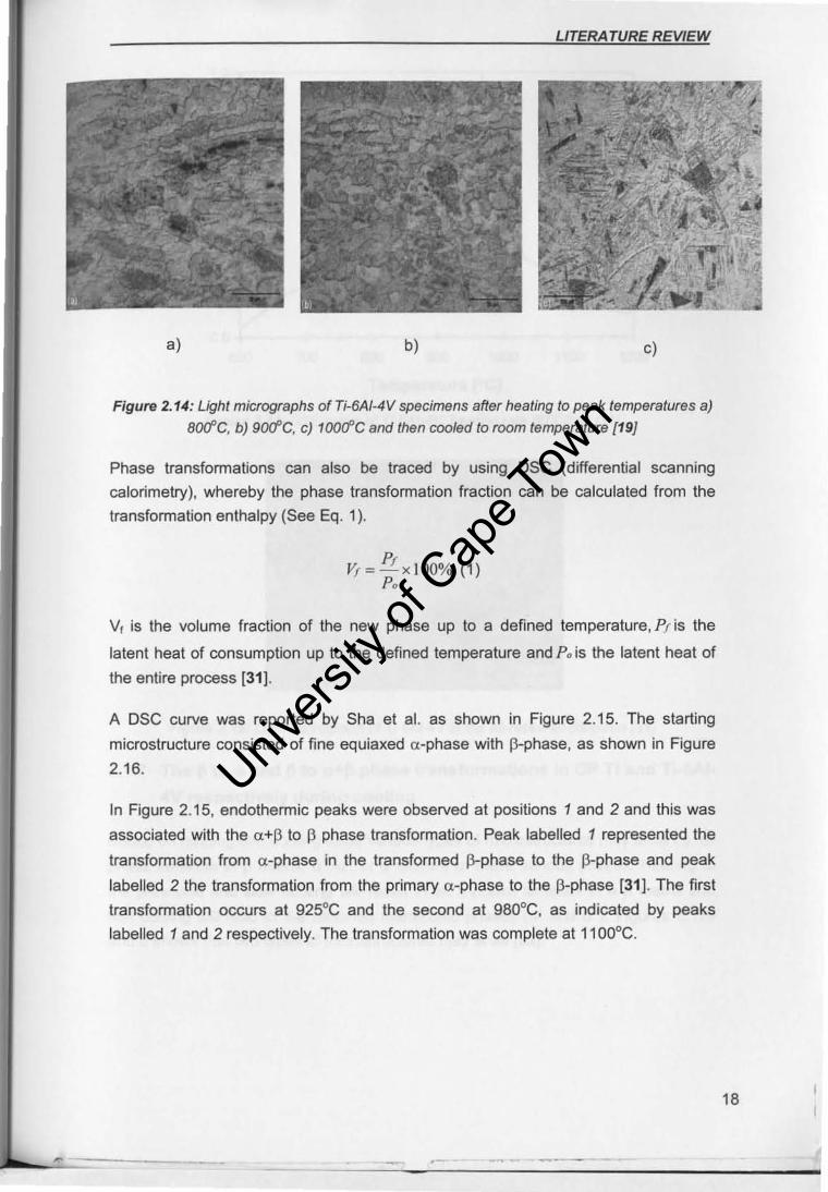
Figure 2.14: Light micrographs of Ti-6AI-4V specimens after heating to peak
temperatures a) 800°C, b) 900°C, c) 1000°C and then cooled to room temperature
[19}. .......................................................................................................................... 18
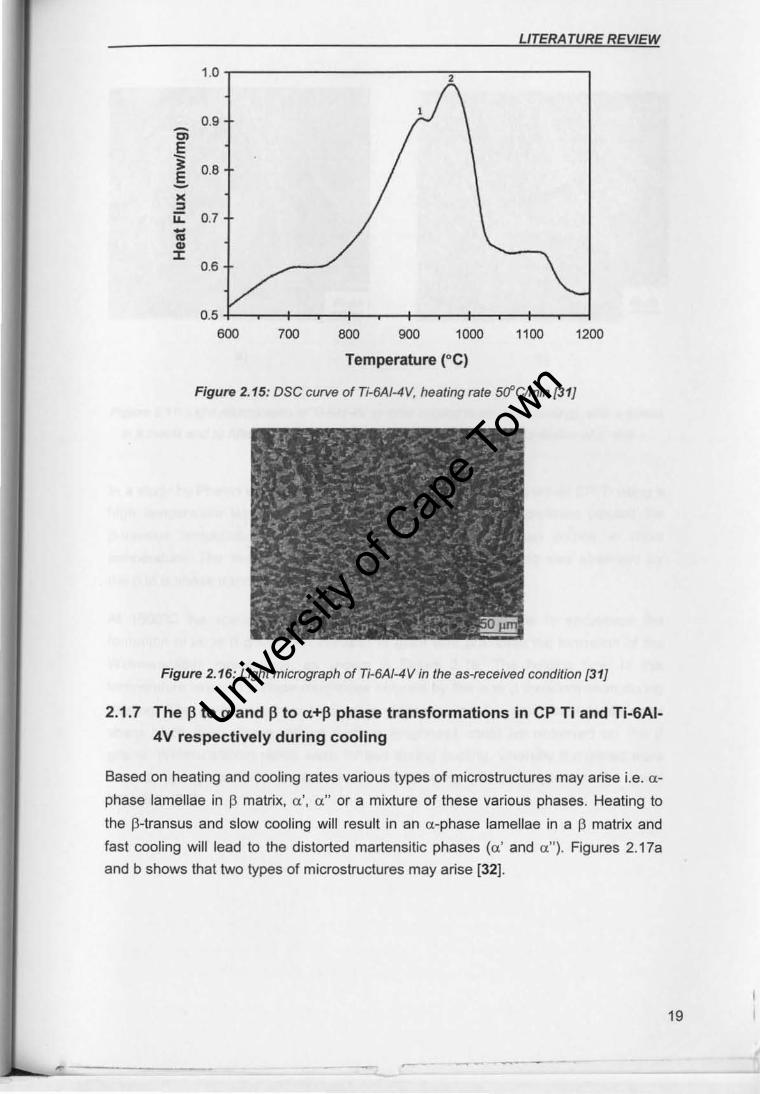
Figure 2.15: DSC curve of Ti-6AI-4V, heating rate 500C/min [31} ............................. 19
Figure 2.16: Light micrograph of Ti-6AI-4 V in the as-received condition [31} ............ 19
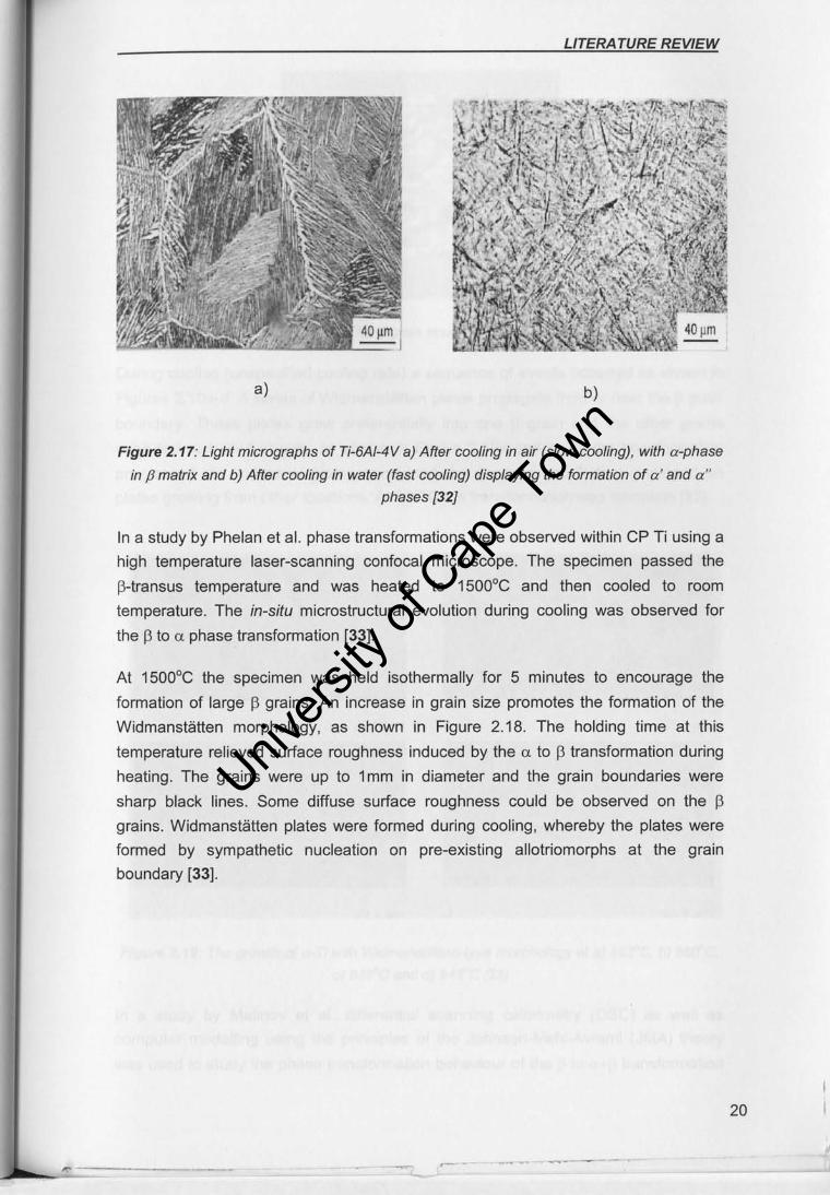
Figure 2.17: Light micrographs of Ti-6AI-4V a) After cooling in air (slow cooling), with
a-phase in fJ matrix and b) After cooling in water (fast cooling) displaying the
formation of a' and a" phases [32} ...................................................................... 20
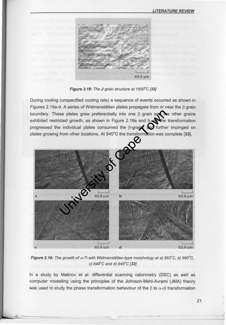
Figure 2. 18: The fJ grain structure at 1500°C [33]. .................................................... 21
Figure 2.19: The growth of a-Ti with Widmanstatlen-type morphology at a) 86~C, b)
860°C, c) 849°C and d) 84~C [33]. .......................................................................... 21
Figure 2.20: Light micrographs of Ti-6AI-4V after continuous cooling (cooling rate
20°C/min) from a) 860°C/min and b) 750°C [26} ....................................................... 22
Figure 2.21: Formation of a mixture of a' and am (a formed by massive
transformation mechanism) cooling rate a) 31500, b) 24600, c) 16500, d) 10500 e)
12000C/min in Ti-6AI-4V[34} ..................................................................................... 24
Figure 2.22: Formation of Widmanstalten, cooling rate a), b) 900°C/min and c)
900C/min in Ti-6AI-4V [34} ........................................................................................ 25
Figure 2.23: Measured lattice parameters as a function of temperature for a) hcp and
b) bcc during heating at 2°C/s and 1O°C/s. The indicated coefficients of thermal
expansion were calculated from the slopes [19]. ...................................................... 26
Figure 2.24: a) Unit cell volume of hcp and bcc phases as a function of temperature
and b) Average cell volume 1/3 ( dilation) as function of temperature [19}. .................. 27
Figure 2.25: Atomic volume of Ti-H phases as a function of H concentration [38} .... 28
Figure 2.26: Hydrogen activity for selected titanium al/oys at 800°C [39}. ................. 29
Figure 2.27: Hydrogen concentration vs. temperature for CP Ti. A saturation of
hydrogen concentration for the temperatures above 600°C was observed [41} ........ 30
viii
JIll!" ------ - -- -
Univers
ity of
Cap
e Tow
n
Figure 2.28: Hydrogen concentration vs. temperature for Ti-6AI-4V. A saturation of
hydrogen concentration for the temperatures above 650°C was observed [41) ........ 30
Figure 2.29: Phase boundaries in Ti-6AI-4V-H system according to a) Kerr et al. [28)
and b) lIyin et al. [27). ............................................................................................... 34
Figure 2.30: Light micrographs of Ti-6AI-4V alloy a)As-cast, b) 10 at%H, c) 20 at%H,
d) 30at%H all at 780°C for 24hours followed by air cooling [6) ................................. 35
Figure 2.31: Light micrographs of Ti-6AI-4V alloy containing 30at% H after heating at
a) 750°C, b) 800°C, c) 83ifC and d) 850°C for 1 hour and water quenching thereafter
[6]. ............................................................................................................................ 36
Figure 2.32: Phase diagram for a) Ti-6AI-4V-H as proposed by Qazi et al. [6) and b)
Ti-H as proposed by Wang et. al. [49) ...................................................................... 38
Figure 2.33: Light micrographs of specimens with 30at% H after annealing for 850°C
for 1 hr followed by annealing at 780°C for a) 16 hr and water quenching and b) 64 hr
and water quenching showing 12vol% transformation [50) ....................................... 39
Figure 2.34: TEM micrograph with 20at% H after annealing for 1 h at 850°C and water
quenching, BF showing titanium hydride laths [50). .................................................. 39
Figure 2.35: TTT diagrams for b phase decomposition in Ti-6AI-4V specimens with a)
10at% H, b) 20at% H and c) 30at%H [6) ................................................................ .40
Figure 2.36: Dependence of the a) nose temperature and b) nose time for the
beginning of the fi phase decomposition on the hydrogen concentration [6]. ........... .41
Figure 2.37: Microstructures of Ti-6AI-4V containing a) Oat% H, b) 11.84at% H, c)
17.3at% H and d) 22. 92at%H quenched from the fi phase field [51) ....................... .43
Figure 2.38: Microstructure of Ti-6AI-4V hydrogenated at 750°C for 1hour followed by
air cooling, samples containing, a) Oat% H, b) 4. 71at% H, c) 11.41at% H and d)
20.07at% H [52) ....................................................................................................... 44
Figure 2.39: Micrograph of bulk 0 TiH2[56]. .............................................................. 45
Figure 2.40: Change in the lattice parameter a of 0 TiH2 with hydrogen concentration
CH [56) ...................................................................................................................... 46
Figure 2.41: Schematic representation of eutectoid transformation mechanism from
fiH to a and 0 during cooling [57) ............................................................................. .47
ix
,... -------------- -----------------~-------------------------.......... ..
Univers
ity of
Cap
e Tow
n
Figure 2.42: Hydrogen diffusion in the eutectoid PH to a+ 0 transformation [57J ...... .47
Figure 4.1: Temperature profile of annealing procedure in vacuum .......................... 51
Figure 4.2: Strain and COTE vs. temperature during heating and cooling of CP Ti,
assuming perfect equilibrium .................................................................................... 53
Figure 4.3: Phase diagram of the Fe-C system ........................................................ 54
Figure 4.4: Expansion behaviour of Iron, 0.1wt% steel at equilibrium and non
equilibrium conditions (theoretical) and experimental ............................................... 56
Figure 4.5: Set up of an EBSD unit .......................................................................... 62
Figure 4.6: An EBSD pattern showing Kikuchi bands ............................................... 63
Figure 5.1: a)Model/ed volume of a and P phases (per atom) as a function of
temperature for CP Ti ............................................................................................... 65
Figure 5.2: CP Ti heated to 1000DC, heating and cooling rate 1DClmin, repeated
thrice (Tests 1, 2 and 3) to illustrate reproducibility of the dilatometry technique . ..... 66
Figure 5.3: Plot of Strain and COTE vs. temperature, Cycles 0-2, during heating of
CP Ti ........................................................................................................................ 72
Figure 5.4: Ti-H phase diagram: Cycle 1 during heating ........................................... 73
Figure 5.5: Plot of Strain and COTE vs. temperature, Cycle 0, 1 and 2 during cooling
ofCP Ti .................................................................................................................... 74
Figure 5.6: Ti-H phase diagram: Cycle 1 during cooling ........................................... 75
Figure 5.7: Ti-H phase diagram: Cycle 2 during heating ........................................... 76
Figure 5.8: Ti-H phase diagram: Cycle 2 during cooling ........................................... 77
Figure 5.9: Plot of Strain and COTE vs. temperature, Cycles 2-4, during heating of
CP Ti ........................................................................................................................ 80
Figure 5.10: Plot of Strain and COTE vs. temperature, Cycles 2-4 during cooling of
CP Ti ........................................................................................................................ 81
Figure 5.11: Plot of Strain and COTE vs. temperature, Cycles 0&4, during heating of
CP Ti ........................................................................................................................ 83
x
Univers
ity of
Cap
e Tow
n
Figure 5.12: Plot of Strain and COTE vs. temperature, Cycle 0 and 4 during cooling
of CP Ti .................................................................................................................... 84
Figure 5.13: Plot of Strain and COTE graphs, Cycles 0, 1 and 2 during heating of Ti-
6AI-4V ...................................................................................................................... 89
Figure 5.14: Plot of Strain and COTE vs. temperature, Cycles 0, 1 & 2 during cooling
of Ti-6AI-4 V ......................................................................................................... 90
Figure 5.15: Plot of Strain and COTE vs. temperature, Cycles 2-4 during heating of
Ti-6AI-4V .................................................................................................................. 93
Figure 5.16: Plot of Strain and COTE vs. temperature, Cycles 2-4, during cooling of
Ti-6AI-4V .................................................................................................................. 94
Figure 5.17: Plot of Strain and COTE vs. temperature, Cycles 0 and 4, during heating
of Ti-6AI-4 V ......................................................... ................................................. 96
Figure 5.18: Plot of Strain and COTE vs. temperature, Cycles 0 and 4, during cooling
of Ti-6AI-4V ......................................................................................................... 97
Figure 5.19: Comparison of Strain and COTE vs. temperature curves during heating
of CP Ti and Ti-6AI-4V, Cycle 0 ................................................................................ 98
Figure 5.20: Comparison of Strain and COTE vs. temperature curves during cooling
of CP Ti and Ti-6AI-4V, Cycle 0 ................................................................................ 99
Figure 5.21: Comparison of Strain and COTE vs. temperature curves during heating
of CP Ti and Ti-6AI-4 V, Cycle 1 .............................................................................. 1 00
Figure 5.22: Comparison of Strain and COTE vs. temperature curves during cooling
of CP Ti and Ti-6AI-4 V, Cycle 1 .............................................................................. 1 01
Figure 5.23: Comparison of Strain and COTE curves during heating of CP Ti and Ti-
6AI-4V, Cycle 2 ...................................................................................................... 102
Figure 5.24: Comparison of Strain and COTE vs. temperature curves during cooling
of CP Ti and Ti-6AI-4V, Cycle 2 .............................................................................. 103
Figure 5.25: Comparison of Expansion and COTE vs. temperature curves during
heating of CP Ti and Ti-6AI-4V, Cycle 3 ................................................................. 104
Figure 5.26: Comparison of Strain and COTE vs. temperature curves during cooling
of CP Ti and Ti-6AI-4V, Cycle 3 .............................................................................. 105
xi
JIll:" -----~-- -
Univers
ity of
Cap
e Tow
n
Figure 5.27: Comparison of Strain and COTE vs. temperature curves during heating
for CP Ti and Ti-6AI-4 V, Cycle 4 ............................................................................ 1 06
Figure 5.28: Comparison of Strain and COTE vs. temperature curves during cooling
for CP Ti and Ti-6AI-4V, Cycle 4 ............................................................................ 1 06
Figure 5.29: Light micrographs of CP Ti after a) Cycle 0 and b) Cycle 4 ................ 1 07
Figure 5.30: a) Light micrograph of CP Ti after Cycle 1, showing a mixture of hydride
and a phases and b) EBSD map, red regions: hcp (ala? phase, yellow and blue
regions: two forms of hydride phases (0 and E), white regions: non-indexed regions
............................................................................................................................... 108
Figure 5.31: CP Ti after 32SOC quench during cooling a) Light micrograph at low
magnification b) high magnification displaying and hcp and hydride phases c) SEM
image of scanned region (selected region highlighted in red) and d) EBSD map of
scanned region, blue and yellow regions: two forms of hydrides (0 and E) ............. 109
Figure 5.32: CP Ti after 750°C quench a) Light micrograph at low magnification
displaying large a-grains and smaller fJ-grains b) SEM image of scanned region
(selected region highlighted in red) and c) EBSD map of scanned region, red region:
hcp phase (ala?, yellow and blue regions: two forms of hydrides (0 and E) ............ 110
Figure 5.33: a) Light micrograph of CP Ti after 82SOC quench, displaying an equiaxed
grain structure with a mixture of a hcp (ala? and hydride phases b) SEM image of
scanned region (selected region highlighted in red) displaying distinct grains and c)
EBSD map of scanned region displaying the composition of the grains, red regions:
hcp (ala? phase, yellow and blue regions: two forms of hydride phases (0 and E), and
white regions: non indexed regions ........................................................................ 112
Figure 5.34: a) CP Ti after 940°C quench a) Light Micrograph at low magnification
and b) high magnification c) SEM image of scanned region (selected region
highlighted in red), d) EBSD image of scanned region in (c), red region: hcp (ala?
phase, white regions: non-indexed regions, e) SEM image of a different region within
the specimen (at higher magnification) and f) EBSD image of scanned region in (e),
yellow and blue regions: two forms of hydride phases (0 and E) ............................. 114
Figure 5.35: Light micrograph of Ti-6AI-4V after Cycle 0, displaying Widmanstatten
plates and the prior fJ grain boundary ..................................................................... 115
Figure 5.36: Light micrograph of Ti-6AI-4V after 1000°C quench, displaying
martensite (a? needles .......................................................................................... 116
xii
Univers
ity of
Cap
e Tow
n
Figure 5.37: Ti-6AI-4Vafter Cycle 1 a) Light micrograph and b) EBSD map, red
regions: hcp (ala') phase, yel/ow regions: f3 phase, white regions: non-indexed
regions ............................... .................................................................................... 117
Figure 5.38: Ti-6AI-4Vafter Cycle 2 a) Light micrograph b) EBSD map, red regions:
hcp (ala') phase, yel/ow regions: f3 phase, white regions: non-indexed regions ..... 118
Figure 5.39: Ti-6AI-4Vafter Cycle 3 a) Light micrograph b) EBSD map, red regions:
hcp (ala') phase, yel/ow regions: f3 phase, white regions: non-indexed regions ..... 119
Figure 5.40: Ti-6AI-4V after Cycle 4 a) Light micrograph showing coarse a grains in a
f3 matrix b) EBSD map, red regions: hcp (ala') phase, yel/ow regions: f3 phase, white
regions: non-indexed regions and black regions: grain boundaries ........................ 120
xiii
Univers
ity of
Cap
e Tow
n
INTRODUCTION
1 INTRODUCTION
1.1 Subject of research
This project deals with monitoring the phase transformations and microstructural
evolution in wrought commercially pure titanium (CP Ti) and the Ti-6AI-4V alloy,
utilising hydrogen as a temporary alloying element with in situ dilatometry during
hydrogen purging.
1.2 Background to research
Hydrogen is used as a temporary alloying element since it can be easily added and
removed without melting. Titanium and its alloys have a high affinity for hydrogen and
are able to absorb up to 60at% from temperatures 600°C and greater [1].
Hydrogen utilised during various heat treatments of CP Ti and Ti-6AI-4V alloy, lowers
the l3-transus temperature in order to refine the microstructure and hence, improves
the mechanical properties at a lower cost. This type of processing is called
thermohydrogen processing (THP) [1]. The hydrogen within the alloy works by
modifying phase compositions, developing of metastable phases and altering the
kinetics of phase transformations [1]. The decomposition of the metastable phases
results in the refinement of the microstructure. However, contents of greater 0.02ppm
of hydrogen remaining within the metal can be detrimental and leads to degradation
in fracture related mechanical properties [2]. The removal of hydrogen after
processing is thus critical in order to avoid this degradation. Removal of hydrogen is
achieved by vacuum annealing where the reaction of hydrogen with the alloy is
reversible owing to its positive enthalpy of solution in titanium [3].
Hydrogen is capable of destabilising the low temperature a phase and stabilising the
more ductile high temperature 13 phase in the alloy [4]. Therefore when hydrogen is
added the a-phase transforms partly into the l3-phase above the eutectoid
temperature, the temperature of transforming a to 13 phase is lowered and the
temperature interval of the two phase (a+l3) is increased [1].
The decrease in the temperature range of the (a+l3) to 13 transformation by the
addition of hydrogen, leads to a reduction in grain growth on heating into the modified
13 range [5]. The hydrogen-induced increase in the temperature interval of the a+13
range allows heat treatments to be performed that would not have been possible
without the addition of hydrogen. These factors in turn leads to different
microstructures in the conventional Ti-6AI-4V alloy [5].
~ ------- -..
1
Univers
ity of
Cap
e Tow
n
INTRODUCTION
An increase in the more workable 13-phase improves hot-workability of the alloy and
decreases the hot working temperatures. The shear modulus of the 13-phase
increases due to hydrogen affecting dislocation interactions and thus strengthening
the 13-phase.
Hydrogen addition to the alloy decreases the 13 to a+13 transus temperature, which
then reduces the critical cooling rate required for martensite formation [6].
The conventional method of thermo hydrogen processing involves i) 13 solution
treatment before, during or after hydrogenation, ii) aging treatment below the
hydrogenated 13-transus for thermomechanical processing and finally iii)
dehydrogenation by vacuum annealing at a lower temperature [7].
1.3 Objectives of the research
The objectives of the research are to:
• Successfully modify the push-rod dilatometer to act as a dual functioning
dilatometer/hydrogen furnace
• Monitor the phase transformation behaviour of CP Ti and the Ti-6AI-4V alloy
using the dual functioning dilatometer before, during and after hydrogenation
• Use the temporary alloying abilities of hydrogen to alter the kinetics and
phase transformations of the stable CP Ti and Ti-6AI-4V alloy
• Determine the phases formed before, during and after hydrogenation
• Compare the phase transformation behaviour of CP Ti and Ti-6AI-4V before,
during and after hydrogenation
• Monitor the absorption-desorption behaviour of hydrogen in CP Ti and Ti-6AI-
4V and hydride formation/decomposition
1.4 Scope and limitations
The main material for this project is Ti-6AI-4V. Experiments were also performed on
CP Ti to serve as a bench mark for Ti-6AI-4V. The focus of the project is to monitor
the real-time phase transformations of both CP Ti and Ti-6AI-4V before, during and
after hydrogenation using dilatometry. The mechanical properties arising from the
different heat treatments with hydrogen and in vacuum were not evaluated. The
project also focuses on the phase transformations during continuous heating and
cooling. Isothermal phase transformations were not considered.
2
Univers
ity of
Cap
e Tow
n
INTRODUCTION
1.5 Plan of development
The project has been presented in a particular sequence. The first chapter is aimed
to introduce the reader to the research project. The second chapter is a review of
past research that has been conducted on heat treating and thermohydrogen
processing of titanium alloys. The third chapter describes the redesign and
modification of the testing facility and the fourth chapter the experimental procedure.
The results and discussion are presented in chapter five, with conclusions in chapter
six and finally future work in chapter seven.
3
Univers
ity of
Cap
e Tow
n
LITERATURE REVIEW
2 LITERATURE REVIEW
2.1 Material
2.1.1 The history of titanium
Prior to World War II, titanium was merely a curiosity to metallurgists, though it had
the potential for great strength and light weight properties. Titanium in its natural form
i.e. titanium oxide (rutile Ti02) had limited applications, such as an additive to paint. It
was only after the end of the Cold War that titanium expanded from military use to
commercial applications, including artificial hips, golf clubs, tennis rackets, bicycles
and wedding rings. Titanium is as strong as steel, yet it is 45% lighter and is twice as
strong as aluminium and only 60% heavier. It is biologically inert, making it ideal for
implants for the body. It also does not corrode in naturally corroding environments,
therefore it may be used for sea submersibles, heat exchangers and a variety of
chemical plant applications [8].
Titanium is difficult to obtain from its ore which commonly occurs as "black sand".
Transforming this black sand into a usable material is a complicated and expensive
process. William Kroll, a metallurgist developed the Kroll process whereby rutile
titanium is converted to titanium tetrachloride and then reacts with magnesium or
sodium to produce titanium [8].
2.1.2 Introduction to titanium and its alloys
Titanium is classified as a lightweight, corrosion resistant material. The material can
be strengthened through alloying and heat treating. Titanium has the following
properties:
• Good strength to weight ratio
• Low density
• Low coefficient of thermal expansion
• Good corrosion resistance
• Good toughness
• Good oxidation resistance at intermediate temperatures
Titanium is commonly used in the aerospace (for jet engines and airframe
components) and marine industries due to the above properties and it is a
representative material in modern turbine engines. Usage is also widespread in most
,...-----
4
Univers
ity of
Cap
e Tow
n
LITERATURE REVIEW
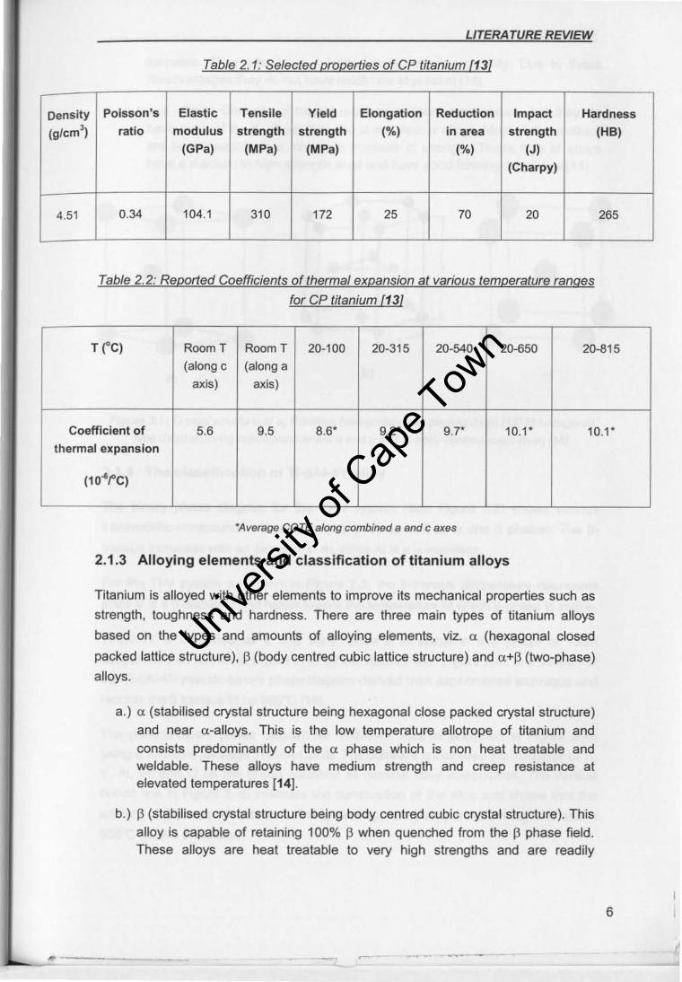
commercial and military aircraft. Its properties, as shown in Table 2.1 is what makes
this metal highly versatile in industry [9].
Titanium alloys are determined by their alloying contents and heat treatments. Pure
titanium has an "alpha" (a) structure up to 883°C and above this temperature it
transforms to the "beta" (13) structure. This temperature is known as j3-transus
temperature [10]. These two phases exhibit different properties due to their different
crystal structures. Table 2.1 lists some properties of CP Ti and Table 2.2 lists
coefficients of thermal expansion at varying temperatures.
CP Ti exhibits a hcp crystal structure (See Figures 2.1 a and b) and the coefficients of
thermal expansion for the basal plane (along the a axis) will differ from the adjacent
plane (along the c axis) (See Table 2.2) [11]. The difference in these coefficients of
thermal expansion (COTE) values can be attributed to the fact that the binding
between the neighbouring atoms in the basal plane is weaker than the adjacent
planes, and hence atomic displacements due to temperature increase will be easier
and larger along the a axis than along the c axis. Boyer et al. however, makes
mention that the COTE values for the adjacent plane are reported to be 20% greater
than that of the basal plane [12]. Hence, there is a discrepancy for the difference in
COTE values in the basal and adjacent planes in the hcp crystal lattice. For the
purpose of this research, only average COTE values along combined a and c axes
were considered.
The addition of a stabilising elements such as (AI, Ga, Sn) increases the temperature
of allotropic transformation and the addition of 13 stabilising elements such as (V, Nb
and Ta) reduces the temperature of the allotropic transformation. Through various
thermal treatments and the addition of alloying elements, various microstructures
resulting in different mechanical properties may be obtained.
Alloying elements are either classified as a or j3 stabilizers
• a stabilizers increases the temperature at which the a phase is stable, e.g. AI, Ga, Ge, C, O2, N2, Sn, Zr
• j3 stabilisers decreases the temperature at which the j3 phase is stable, e.g. Mo, V, Ta, Fe, Cr, Si, Ni, Cu, H2
,... ------ - -- ---
5
Univers
ity of
Cap
e Tow
n
LITERA TURE REVIEW
Table 2.1: Selected properties of CP titanium [131
Density poisson's Elastic Tensile Yield Elongat ion Reduction Impact Hardness
(g/cm')
4.51
ratio modulus strength strength (%) in area strength
(GPa) (MPa) (MPa) (%) (J)
(Charpy)
0.34 104.1 310 172 25 70 20
Table 2.2: Reported Coefficients of thermal expansion at various temperature ranges
for CP titanium (13/
(HB)
265
T (0G) Room T RoomT 20-100 20-315 20-540 20-850 20-815 (along c (along a
axis) axis)
Coefficient of 5.6 9.5 8.6' 9.2' 9.1' 10.1' 10.1' thermal expansion
(10<rc)
·Average COTE along combined 8 and c axes
2.1.3 Alloying elements and classification ofiitanium alloys
Titanium is aUoyed with other elements to improve its mechanical properties such as
strength, toughness and hardness. There are three main types of titanium alloys
based on the types and amounts of alloying elements. viz. a (hexagonal closed
packed lattice structure), 13 (body centred cubic lattice structure) and a+p (two-phase)
alloys.
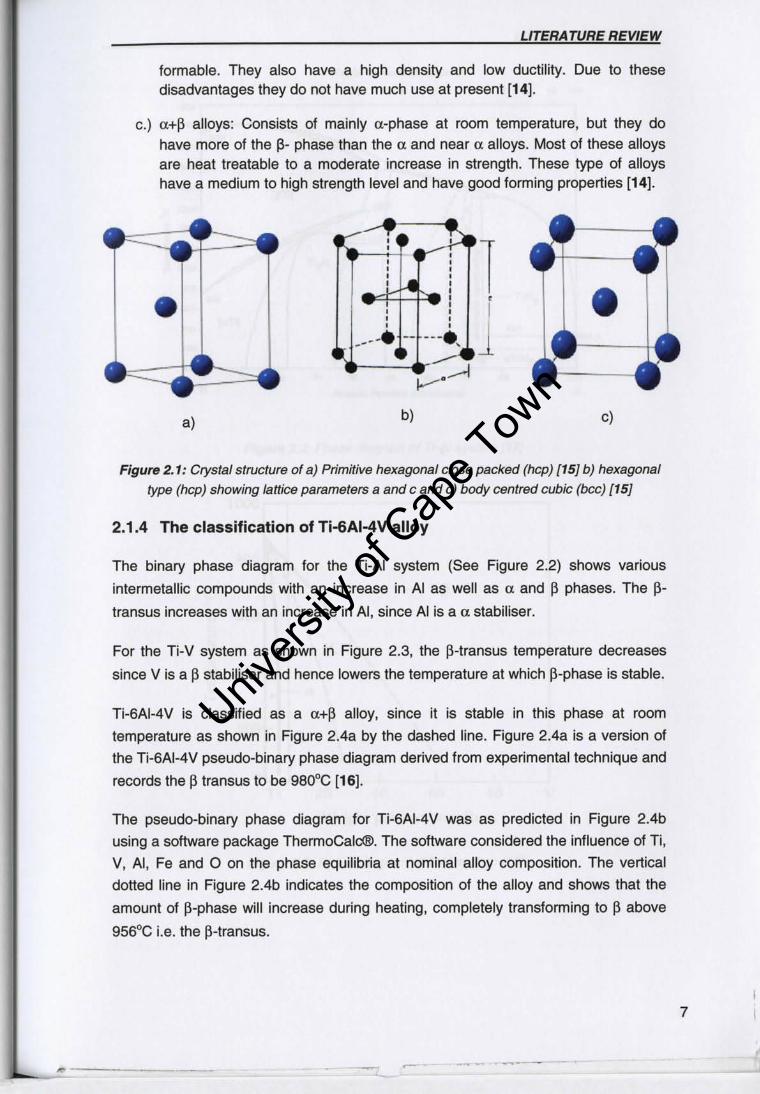
a.} a (stabilised crystal structure being hexagonal close packed crystal structure) and near a-alloys. This is the low temperature allotrope of ti tanium and consists predominantly of the a phase which is non heat treatable and weldable. These alloys have medium strength and creep resistance at elevated temperatures [14).
b.) 13 (stabilised crystal structure being body centred cubic crystal structure). This alloy is capable of retaining 100% j3 when quenched from the J3 phase field. These alloys are heat treatable to very high strengths and are readily
......... ...:: ____ ~o_ ........ ---
6
Univers
ity of
Cap
e Tow
n
LITERATURE REVIEW
formable. They also have a high density and low ductility. Due to these disadvantages they do not have much use at present [14].
c.) a+13 alloys: Consists of mainly a-phase at room temperature, but they do have more of the 13- phase than the ex and near ex alloys. Most of these alloys are heat treatable to a moderate increase in strength. These type of alloys have a medium to high strength level and have good forming properties [14] .
... f ;',. , ... , , i l..4 T • , , ,
, I ,
----.• - ---. , .---'
a) b) c)
Figure 2.1: Crystal structure of a) PrimitivB hexagonal close packed (hcp) (15] b) hexagonal
type (hcp) showing JaNice parameters a and c and cJ body centred cubic (bee) [15J
2.1.4 The classification of Ti-6AI-4V alloy
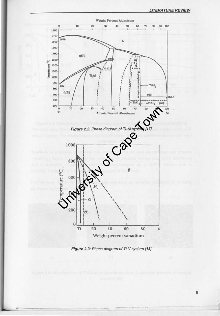
The binary phase diagram for the Ti-AI system (See Figure 2.2) shows various
intermetallic compounds with an increase in AI as well as a and ~ phases. The ~
transus increases with an increase in AI , since AI is a a stabiliser.
For the Ti-V system as shown in Figure 2.3, the ~-transus temperature decreases
since V is a ~ stabiliser and hence lowers the temperature at which ~-phase is stable.
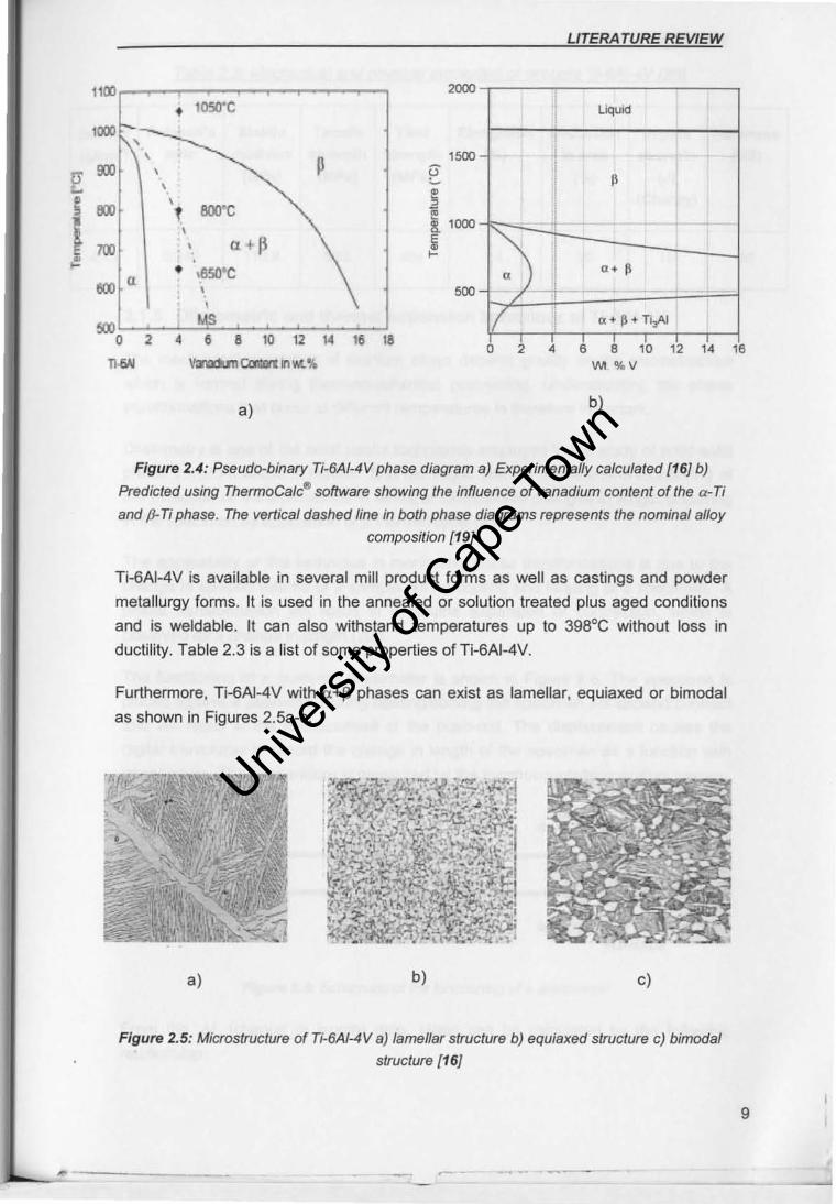
Ti-6AI-4V is classified as a a+~ alloy, since it is stable in this phase at room
temperature as shown in Figure 2.4a by the dashed line. Figure 2.4a is a version of
the Ti-6AI-4V pseudo-binary phase diagram derived from experimental technique and
records the ~ transus to be 980' C [16].
The pseudo-binary phase diagram for Ti-6AI-4V was as predicted in Figure 2.4b
using a software package ThermoCalC®. The software considered the influence of Ti,
V, AI, Fe and 0 on the phase equilibria at nominal alloy composition. The vertical
dotted line in Figure 2.4b indicates the composition of the alloy and shows that the
amount of ~-phase will increase during heating, completely transforming to ~ above
956°C i.e. the ~-transus.
7
Univers
ity of
Cap
e Tow
n
LITERA TURE REVIEW
Wd&ht Pen:ent Aluminum
• .. .. .. .. 60 70 I!lO 90 100
L
(lml , I> -" 'a; ..... ~l
" I\, \, , : ~ ........ , " I: ¥' , , " , , " ,
" :' , , , 0' , : :: i ""'> , .00 , , ,0 , , , 700
, , . ." , , . , , . •• "" 0 ,
:::TiAi -----------, UTWl (A~ ,
"" i. io • ., 30 .. .. '" .. '" 000 Ti Atomic Percent Aluminum AI
Figure 2.2: Phase diagram of Ti-AI system [17l
1000 1 1 1
800 1
\ ~
U \ 1\ • 1\
~ 600 I \ " ( '" , -'" I \ M, , k
I " \ , 0- 400 1 E 1 \
, \
" H-- a \ , f- 1 \ \
1 \ , 200 1 \ 8% \ \
1 \ \ 1 \ \
0 1
.1 I
Ti 20 40 60 80 V
Weight percent vanadium
Figure 2.3: Phase diagram of Ti-V system {f8]
8
Univers
ity of
Cap
e Tow
n
LITERATURE REVIEW
1100 2000
• 10s0-e ,000 I Liquid
, , '500 ,
P 0' 900 , IT , '-r ! ~ ...
i I"'
• 900 \
~ , &XrC 8. 1000
100 (l ' ~ ~ • ,6SO·C a
IlOO , 500 \
IlOO
I ,
-) i
I a. ~
! (
, ! a+ ~ + Ti~
2 • • • 0 ' 0 '2 " ,. I. '-a 2 4 6 8 10 12 14 18
n .... V:n:du1l ccmn In 1M. "4 WI %V
a) b)
Figure 2.4; Pseudo-binary Ti-6AI-4V phase diagram a) Experimentally calculated {16} b)
Predicted using ThermoCafc$ software showing the influence of vanadium content o f the a-Ti
and p. Ti phase. The vertical dashed line in both phase diagrams represents the nominal atloy
composition [19J
Ti-6AI-4V is available in several mill product forms as well as castings and powder
metallurgy forms. It is used in the annealed or solution treated plus aged conditions
and is weldable. It can also withstand temperatures up to 398°C without loss in
ductility. Table 2.3 is a list of some properties of Ti-6AI-4V.
Furthermore, Ti-6AI-4V with cx+J3 phases can exist as lamellar, equiaxed or bimodal
as shown in Figures 2.5a-c.
a) b) c)
F;gure 2.5: Microstructure of Ti·6AI-4V a) lamellar structure b) equiaxed structure c) bimodal
structure [16J
•
9
Univers
ity of
Cap
e Tow
n
LITERATURE REVIEW
Table 2.3: Mechanical and phvsical properties of wroughl Ti·6AI-4V [201
Density Poisson's Elastic Tensile Yield Elongation Reduction Impact Hardness
(glom' ) ratio modulus strength strength (%) in area strength (HB)
4.43
(GPo) (MPo) (MPo) (%) (J)
(Chorpy)
0.342 11 3.8 993 924 14 30 19
2.1.5 Dilatometric and thermal expansion behaviour of Ti-l;AI-4V
The mechanical properties of titanium aUoys depend greatly on the microstructure
which is formed during thermomechanical processing. Understanding the phase
transformations that occur at different temperatures is therefore important.
Dilatometry is one of the most useful techniques employed in the study 01 solid·solid
phase transformations in metals. This technique permits the real-time monitoring of
the evolution of transformations in terms of dimensional changes in length occurring
in the specimen by application of a thermal cycle [21).
The applicability of this technique in monitoring phase transformations is due to the
change in specific volume of a sample during cooling and heating of a specimen. A
phase transformation will result in a volume expansion or contraction, which is
observed as a change in length (M ).
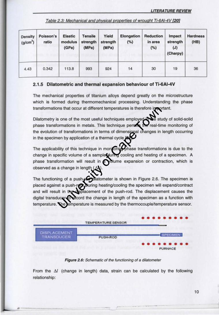
The functioning of a push-rod dilatometer is shown in Figure 2.6. The specimen is
placed against a push-rod. During heating/cooling the specimen will expand/contract
and will result in the displacement of the push-rod. The displacement causes the
digital transducer to record the change in length of the specimen as a function with
temperature. The temperature is measured by the thermocouple/temperature sensor.
DISPLACEMENT TRANSDUCER
TEMPERATURE SENSOR
PUSH-ROD
• • • • • • • • •
SPECIMEN
••••••••• FURNAC E
F;gure 2.6: Schematic of the functioning of a dilatometer
From the l1J (change in length) data, strain can be calculated by the following
relationship:
36
10
Univers
ity of
Cap
e Tow
n
LITERATURE REVIEW
Strain = ~ , where I is the initial length.
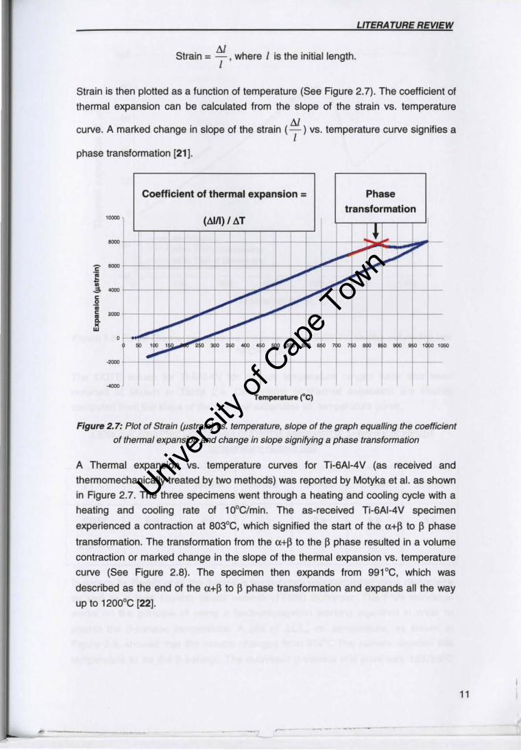
Strain is then plotted as a function of temperature (See Figure 2.7). The coefficient of
thermal expansion can be calculated from the slope of the strain vs. temperature
curve. A marked change in slope of the strain ( 61 ) vs. temperature curve signifies a I
phase transformation [21).
Coefficient of thermal expansion = Phase
transformation ,=
"'" .. "'" :; .; -~ • = ~ w
" .=
(AlII) I <1T
.~ l,. ...... ,..
-
.... r-- !-'"
~ ~ ......
.... .... .... :,.... .... r' .... f"
t.... .... , ,
"" io ... i" "" io .... ,. , . ~ ....
-- I I
Figure 2.7: Plot of Strain (pstrain) vs. temperature, slope of the graph equalling the coefficient
of thermal expansion and change in slope signifying a phase transformation
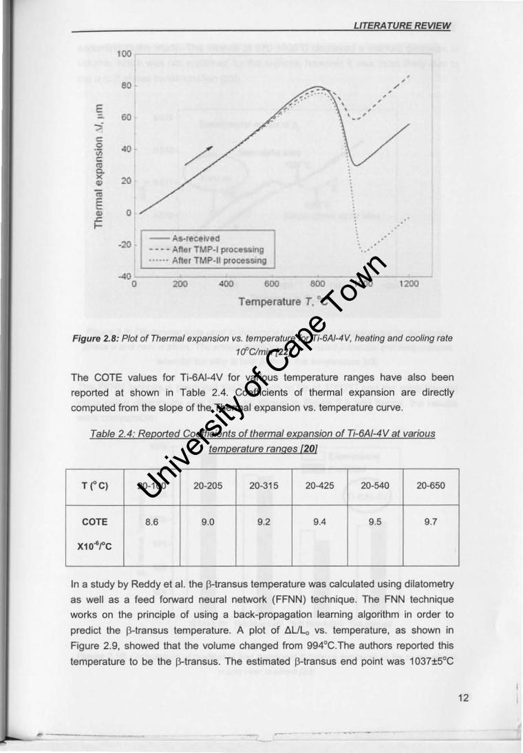
A Thermal expansion vs. temperature curves for Ti-6AI-4V (as received and
thermomechanically treated by two methods) was reported by Motyka et al. as shown
in Figure 2.7, The three specimens went through a heating and cooling cycle with a
heating and cooling rate of 1 DOC/min. The as-received Ti-SAI-4V specimen
experienced a contraction at 8D3°C, which signified the start of the a+p to ~ phase
transformation. The transformation from the a+~ to the p phase resulted in a volume
contraction or marked change in the slope of the thermal expansion vs. temperature
curve (See Figure 2.8). The specimen then expands from 991°C, which was
described as the end of the a+p to p phase transformation and expands all the way
up to 1200"C [22).
11
Univers
ity of
Cap
e Tow
n
LITERA TURE REVIEW
100
, 80 .- ,
-, .. , ........ , , E .. , ,
60 • , - .. -.: ~
" .~ 40 c: '" Co x 20 · '" '" · E · ~
'" 0 ~ f- · ·
- As·recelved · ·20 · - - - - Ane, TMP-I processing .. ...... An., nAp·1I processmg
-40 ,
0 200 ..., 600 600 1000 1200
Temperature T. ClC
Figure 2.8: Plot of Thermal expansion vs. temperature (or Ti-6AJ-4V, heating and cooling rate
II1'Clmin 1221
The COTE values for Ti-6AI-4V for various temperature ranges have also been
reported at shown in Table 2.4. Coefficients of thermal expansion are directly
computed from the slope of the Thermal expansion vs. temperature curve.
Table 2.4: Reported Coefficients of thermal expansion of Ti-6A/-4 V at various
temperature ranges [20]
T (' C) 20-100 20-205 20-315 20-425 20·540 20-650
COTE 8,6 9,0 9,2 9.4 9.5 9.7
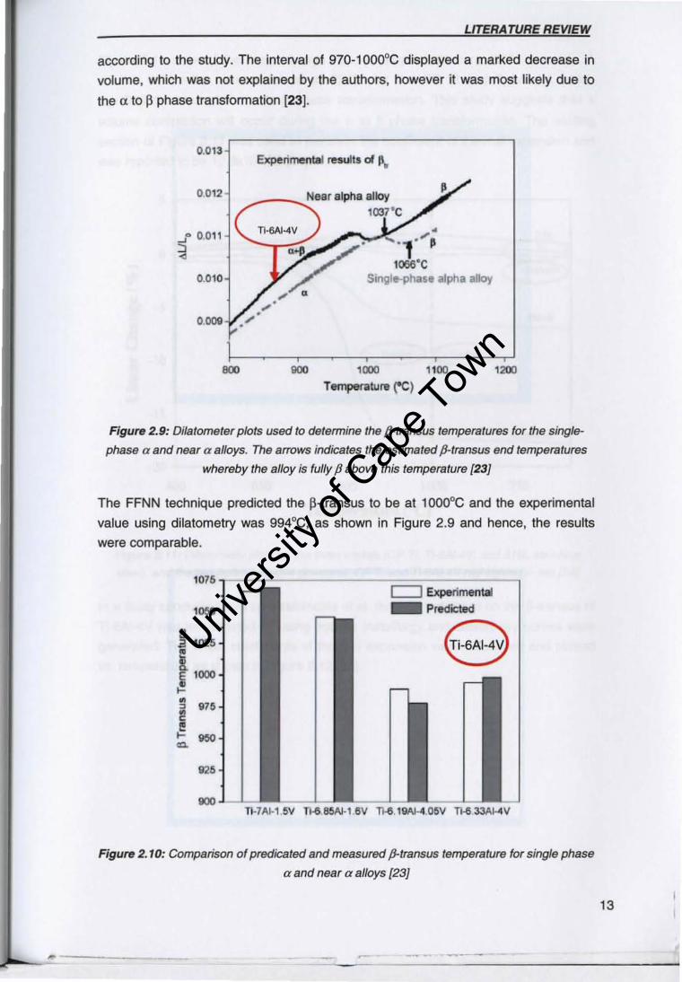
In a study by Reddy et at the fJ-transus temperature was calculated using dilatometry
as well as a feed forward neural network (FFNN) technique. The FNN technique
works on the principle of using a back-propagation learning algorithm in order to
predict the p-transus temperature. A plot of ft.ULo vs. temperature, as shown in
Figure 2.9, showed that the volume changed from 994°C.The authors reported this
temperature to be the I3-transus. The estimated f3-transus end point was 1037±5°C
12
Univers
ity of
Cap
e Tow
n
LITERA TURE REVIEW
according to the study. The interval of 970-1000DC displayed a marked decrease in
volume, which was not explained by the authors, however it was most likely due to
the a to ~ phase transformation [23J.
0.0 13
_I' 0.011
=il
000
Experimental results d fl.
1000
TlII11pOf"Owro ('C) 1100 1200
Figure 2.9: Oi/atometer plots used to determine the p.transus temperatures for the single
phase a and near a alloys. The arrows indicates the estimated p.transus end temperatures
whereby the alloy is fully P above this temperature [23}
The FFNN technique predicted the p-transus to be at 1000°C and the experimental
value using dilatometry was 994°C, as shown in Figure 2.9 and hence, the results
were comparable.
1076
1050
~ 1025
i 1000 1-~
.75 ~ ~ <C.
950
92"
900
c::::J Expefimen1ai _ Predicted
~;I~
TI-1A1-1 SV n.& 85A1-1 8V ll-6.1VA1-4.0SV n.6 33AI .... V
Figure 2. 10: Comparison of predicated and measured p.transus temperature for single phase
a and near a alloys [231
13
Univers
ity of
Cap
e Tow
n
LITERA TURE REVIEW
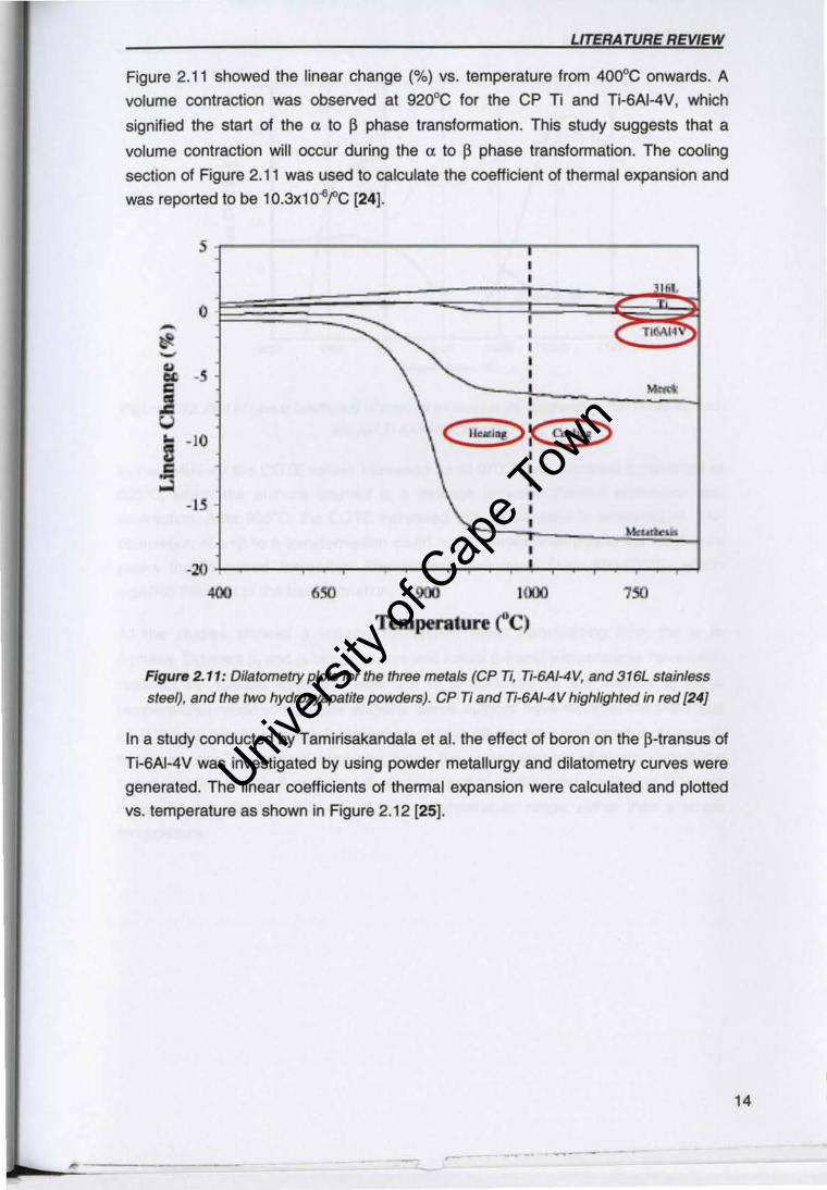
Figure 2.11 showed the linear change (%) liS. temperature from 400°C onwards. A
volume contraction was observed at 920°C for the CP Ti and Ti-SAI-4V I which
signified the start of the ex to ~ phase transformation. This study suggests that a
volume contraction will occur during the ex to ~ phase transformation. The cooling
section of Figure 2.11 was used to calculate the coefficient of thermal expansion and
was reported 10 be IO.3x10~t'C [24] .
5 ~-------------------,----------~
0 ~
~ .. -S ..,
" ...... J 0 u C IO~I'!):<: Odm.:) .... -10 1I " -..l
- IS
-w+-----~--~~---r~~~~_r~~~ __ _r~ 400 6SO 900 1000 7SO
Temperalure I'C)
Figure 2.11: Dilatometry plots for the three metals (ep Ti, Ti·6AI-4V, and 316L stainless
steel), and the two hydroxyapatite powders). CP Ti and Ti-6AI-4V highlighted in red (24]
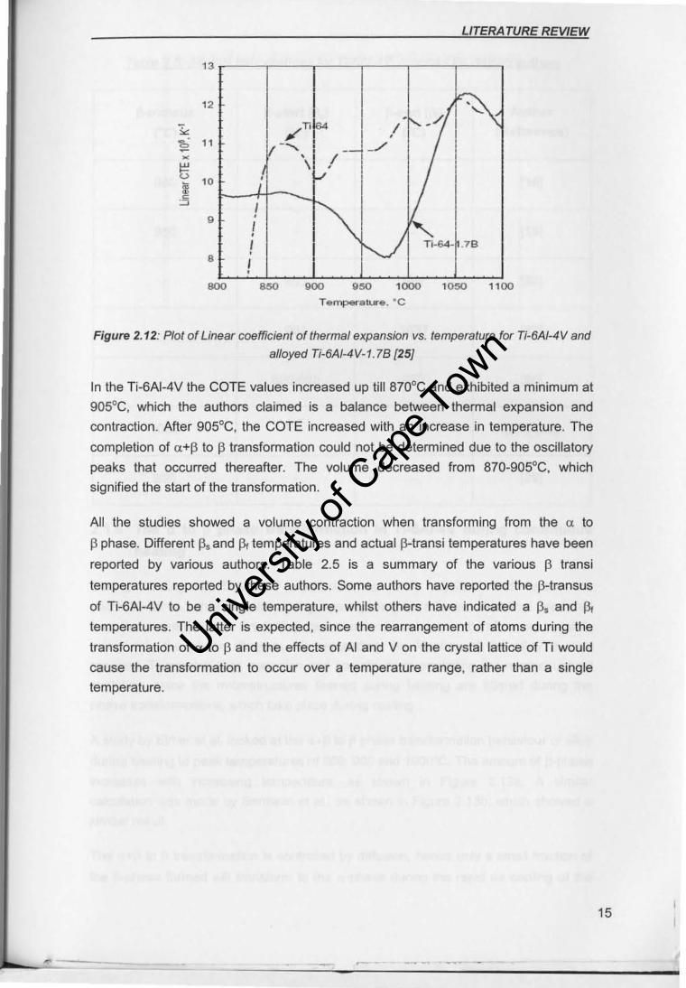
In a study conducted by Tamirisakandala et aL the effect of boron on the p-transus of
Ti-SAI-4V was investigated by using powder metallurgy and dilatometry curves were
generated. The linear coefficients of thermal expansion were calculated and plotted
vs. temperature as shown in Figure 2.12 [25].
14
Univers
ity of
Cap
e Tow
n
LITERA TURE REVIEW
13
12
"'" ~ 11 K
t; 10 ~
/Ti ~ --... .
I \ ,I
~ c
:=> I • • I • I
8 •
800 850 .00 .50 1000 1050 1100
Temperelure , · C
Figure 2.12: Plot of Linear coefficient of thermal expansion vs. temperature for Ti-6Af-4V and
aI/Dyed Ti-6A1-4V- l . 78 {251
In the Ti-6AI-4V the COTE values increased up till B700C and exhibited a minimum at
90SoC, which the authors claimed is a balance between thermal expansion and
contraction. After 905°C, the COTE increased with an increase in temperature. The
completion of a+13 to 13 transformation could not be determined due to the oscillatory
peaks that occurred thereafter. The volume decreased from 870-905°C, which
signified the start of the transformation.
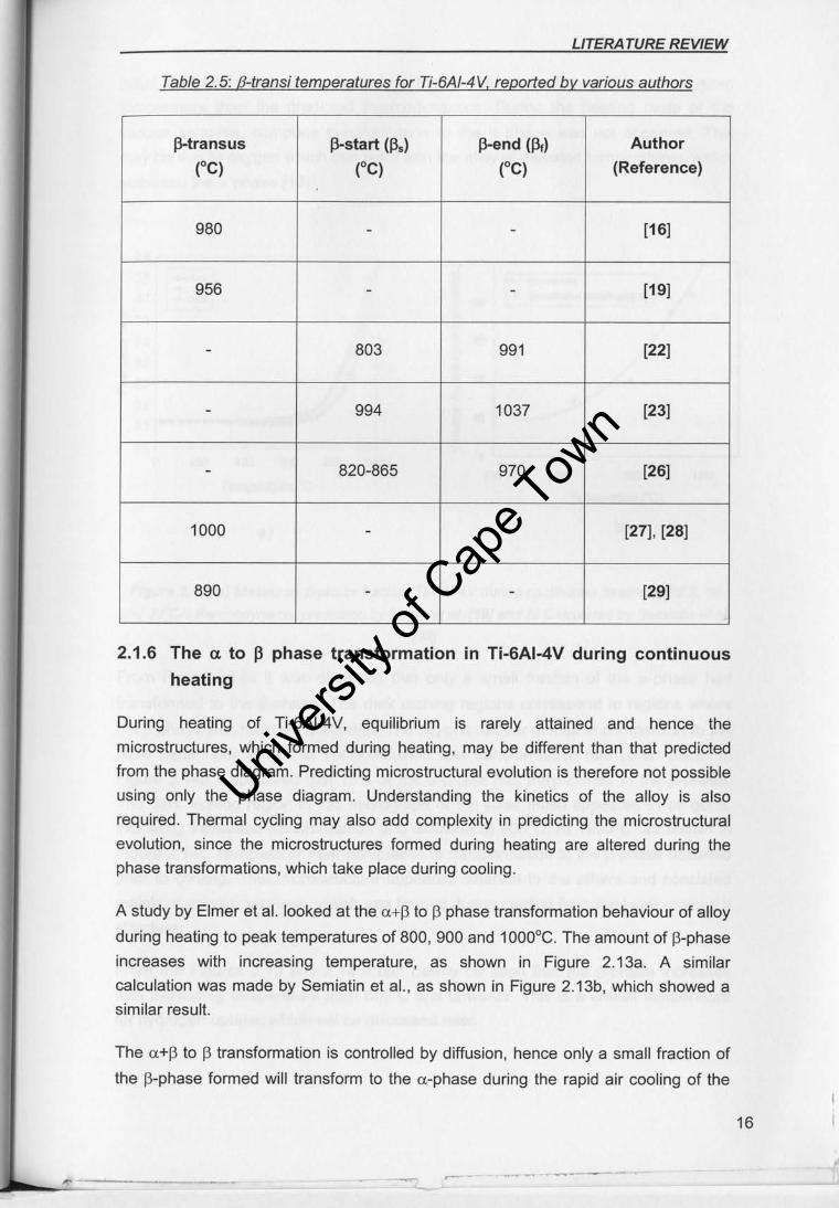
All the studies showed a volume contraction when transforming from the a to
f3 phase. Different f.\ and f3, temperatures and actual p-transi temperatures have been
reported by various authors. Table 2.5 is a summary of the various p transi
temperatures reported by these authors. Some authors have reported the p-transus
of Ti-6AI-4V to be a single temperature, whilst others have indicated a Ps and Pt temperatures. The latter is expected, since the rearrangement of atoms during the
transformation of a to 13 and the effects of AI and V on the crystal lattice of Ti would
cause the transformation to occur over a temperature range, rather than a single
temperature.
15
1
Univers
ity of
Cap
e Tow
n
LITERA TURE REVIEW
Table 2.5: B-transi temperatures for Ti-6AI-4V, reported by various authors
j3-tranSU5 j3-start (Il.) j3-end (Ilt) Author
(OC) (OC) (OC) (Reference)
980 - - [16J
956 - - [19J
- 803 991 [22J
- 994 1037 [23J
- 820-865 970 [26J
1000 - - [27J, [28J
890 - - [29J
2.1.6 The a to p phase transformation in Ti-6AI-4V during continuous
heating
During heating of Ti-6AI-4V, equilibrium is rarely attained and hence the
microstructures, which formed during heating. may be different than that predicted
from the phase diagram. Predicting microstructural evolution is therefore not possible
using only the phase diagram. Understanding the kinetics of the aUoy is also
required. Thermal cycling may also add complexity in predicting the microstructural
evolution, since the microstructures formed during heating are altered during the
phase transformations, which take place during cooling.
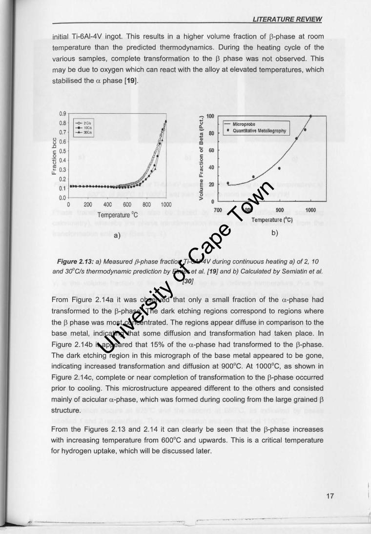
A study by Elmer et aJ. looked at the a+13 to 13 phase transformation behaviour of alloy
during heating to peak temperatures of 800, 900 and 1000oC. The amount of l3-phase
increases with increasing temperature, as shown in Figure 2.13a. A similar
calculation was made by Semiatin et al. , as shown in Figure 2. 13b, which showed a
similar result.
The a+(3 to 13 transformation is controlled by diffusion, hence only a small fraction of
the (3-phase formed will transform to the a-phase during the rapid air cooling of the
16
Univers
ity of
Cap
e Tow
n
1
,
LITERA TURE REVIEW
initial Ti-6AI-4V ingot. This results in a higher volume fraction of l3-phase at room
temperature than the predicted thermodynamics. During the heating cycle of the
various samples, complete transformation to the (3 phase was not observed. This
may be due to oxygen which can react with the alloy at elevated temperatures, which
stabilised the a phase [19] .
0.9 _100 0.6
~ ti - Mlcrop,ot.l
~ , ... .. 0.7 ~ ,.. • 80 • Quantttallw Metallography
.§ 06 ~ • m ~
c 0.5 0 60 0 c n 0.4 ~ • u 40 • ~ 0.3 • "
0.2 ~ • •
0.1 • E 20 , 0.0 g
0 200 400 600 BOO 1000 0
Temperature °c 700 ... 900 1000
Temperature (OCI
a) b)
Figure 2.13: a) Measured (J-phase fraction Ti-6AI-4V during continuous heating a) of 2, 10
and 3(fC/s thermodynamic prediction by Elmer et al. (19] and b) Calculated by Semiatin at af.
[30J
From Figure 2.14a it was observed that only a small fraction of the a-phase had
transformed to the ~-phase. The dark etching regions correspond to regions where
the ~ phase was most concentrated. The regions appear diffuse in comparison to the
base metal, indicating that some diffusion and transformation had taken place. In
Figure 2.14b it appeared that 15% of the a-phase had transformed to the ~-phase.
The dark etching region in this micrograph of the base metal appeared to be gone.
indicating increased transformation and diffusion at 900°C. At 1000oC, as shown in
Figure 2.14c, complete or near completion of transformation to the ~·phase occurred
prior to cooling. This microstructure appeared different to the others and consisted
mainly of acicular a-phase, which was formed during cooling from the large grained ~
structure.
From the Figures 2.13 and 2.14 it can clearly be seen that the ~·phase increases
with increasing temperature from 600°C and upwards. This is a critical temperature
for hydrogen uptake, which will be discussed later.
17
Univers
ity of
Cap
e Tow
n
LITERA TURE REVIEW
a) b) c)
Figure 2.14: Ught micrographs of Ti-6AI-4V specimens after heating to peak temperatures a)
8od'C, b) 9ocfc , c) 100d'C Bnd then cooled to room temperature /19J
Phase transformations can also be traced by using DSC (differential scanning
calorimetry) , whereby the phase transformation fraction can be calculated from the
transformation enthalpy (See Eq. 1).
Pr Vr =-x IOO% (1)
Po
Vf is the volume fraction of the new phase up to a defined temperature, PI is the
latent heat of consumption up to the defined temperature and Po is the latent heat of
the entire process [31).
A DSC curve was reported by Sha et al . as shown in Figure 2.15. The starting
microstructure consisted of fine equiaxed a-phase with (3-phase, as shown in Figure
2.16.
In Figure 2.15, endothermic peaks were observed at positions 1 and 2 and this was
associated with the a+f3 to f3 phase transformation. Peak labelled 1 represented the
transformation from a-phase in the transformed [3-phase to the [3-phase and peak
labelled 2 the transformation from the primary a-phase to the f3-phase (31 ]. The first
transformation occurs at 925°C and the second at 980°C, as indicated by peaks
labelled 1 and 2 respectively. The transformation was complete at 110QoC.
18
Univers
ity of
Cap
e Tow
n
LITERA TURE REVIEW
1.0
0.9 -'" E ~ 0.8 E -.. " LL 0.7 -.. " I
0.6
0.5 800 700 800 900 1000 1100 1200
Temperature (OC)
Figure 2.15: DSC curve of Ti-6AI-4V, heating rate sd'C/min {31]
Figure 2.16: Light micrograph of Ti-6AI-4V in the as-received condition [31]
2.1 .7 The ~ to aand ~ to a+~ phase transformations in CP Ti and Ti·6AI·
4V respectively during cooling
Based on heating and cooling rates various types of microstructures may arise i.e. (X
phase lamellae in p matrix, a ', a" or a mixture of these various phases. Heating to
the IJ-transus and slow cooling will result in an a-phase lamellae in a i3 matrix and
fast cooling will lead to the distorted martensitic phases «(1' and a"). Figures 2.17a
and b shows that two types of microstructures may arise [32).
19
Univers
ity of
Cap
e Tow
n
LITERATURE REVIEW
a) b)
Figure 2.17: Light micrographs of Ti·6AI·4V a) Ahar coofing in air (slow cooling), with a-phase
in p matrix and b) After cooling in water (fast cooling) displaying the formation of a ' and a"
phases {32}
In a study by Phelan et al. phase transformations were observed within CP Ti using a
high temperature laser-scanning confocal microscope. The specimen passed the
~-transus temperature and was heated to 15000 C and then cooled to room
temperature. The in-situ microstructural evolution during cooling was observed for
the p to a phase transformation [33).
At 150QoC the specimen was held isothermally for 5 minutes to encourage the
formation of large p grains. An increase in grain size promotes the formation of the
Widmanstatten morphology, as shown in Figure 2.18. The holding time at this
temperature relieved surface roughness induced by the a to p transformation during
heating. The grains were up to 1 mm in diameter and the grain boundaries were
sharp black lines. Some diffuse surface roughness could be observed on the p
grains. Widmanstatten plates were formed during cooling, whereby the plates were
formed by sympathetic nucleation on pre-existing allotriomorphs at the grain
boundary [33] .
20
Univers
ity of
Cap
e Tow
n
LITERATURE REVIEW
63.9 ~m
Figure 2.18: The p grain structure at 1soCfc {33]
During cooling (unspecified cooling rate) a sequence of events occurred as shown in
Figures 2.1ga-d. A series of Widmanstatten plates propagate from or near the 13 grain
boundary. These plates grew preferentially into one 13 grain and the other grains
exhibited restricted growth, as shown in Figure 2.19a and b. As the transformation
progressed the individual plates consumed the l3-grains and further impinged on
plates growing from other locations. At 845°C the transformation was complete (33].
c L-..J
63.9 urn
b
d
63.91J-m
L-..J 63.9um
Figure 2.19: The growth of a-Ti with Widmanstatten-type morphology at a) 86:fC, b) 86(/'C,
c) 849"C and d) 84if'C 133]
In a study by Malinov et al. differential scanning calorimetry (DSC) as well as
computer modelling using the principles of the JohnsonMMehl·Avrami (JMA) theory
was used to study the phase transformation behaviour of the ~ to a+p transformation
21
Univers
ity of
Cap
e Tow
n
LITERA TURE REVIEW
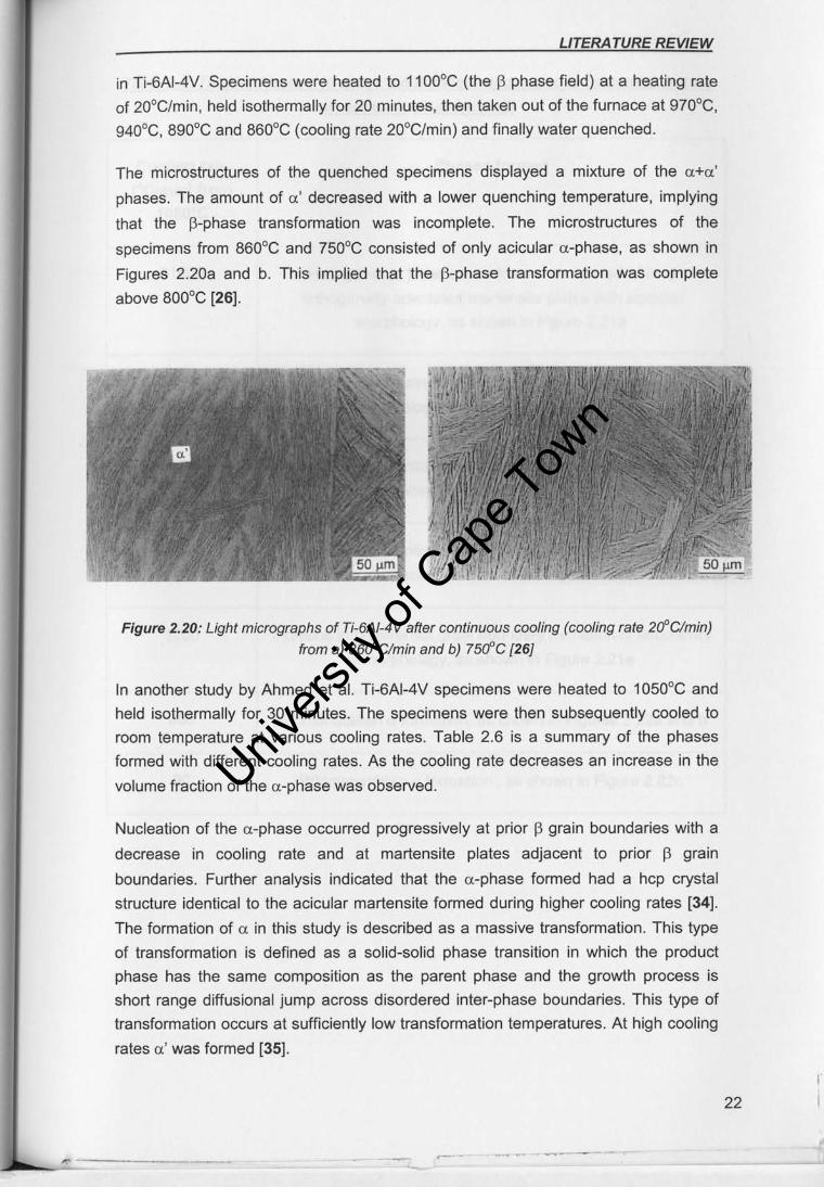
in Ti-6AI-4V. Specimens were heated to 11 DODe (the f3 phase field) at a heating rate
of 20°C/min, held isothermally for 20 minutes, then taken out of the furnace at 970De, 940°C, 8g0De and B60De (cooling rate 20°C/min) and finally water quenched.
The microstructures of the quenched specimens displayed a mixture of the 0.+0.'
phases. The amount of a' decreased with a lower quenching temperature, implying
that the f3-phase transformation was incomplete. The microstructures of the
specimens from B60De and 750°C consisted of only acicular a -phase, as shown in
Figures 2.20a and b. This implied that the l3-phase transformation was complete
above BOO' C [26J.
Figure 2.20: Ught micrographs of fi.6AI-4V after continuous cooling (cooling rate 2(fClmin)
from aJ 86rf'Clmin and bJ 7Srf'C [26J
In another study by Ahmed et aL Ti·6AJ·4V specimens were heated to 10500 C and
held isothermally for 30 minutes. The specimens were then subsequently cooled to
room temperature at various cooling rates. Table 2.6 is a summary of the phases
formed with different cooling rates. As the cooling rate decreases an increase in the
volume fraction of the a·phase was observed.
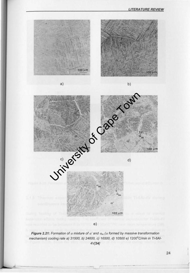
Nucleation of the a-phase occurred progressively at prior p grain boundaries with a
decrease in cooling rate and at martensite plates adjacent to prior p grain
boundaries. Further analysis indicated that the a·phase formed had a hcp crystal
structure identical to the acicular martensite formed during higher cooling rates [34).
The formation of a in this study is described as a massive transformation. This type
of transformation is defined as a solid-solid phase transition in which the product
phase has the same composition as the parent phase and the growth process is
short range diffusional jump across disordered inter·phase boundaries. This type of
transformation occurs at sufficiently low transformation temperatures. At high cooling
rates a' was formed [35].
r 22 I
Univers
ity of
Cap
e Tow
n
LITERA TURE REVIEW
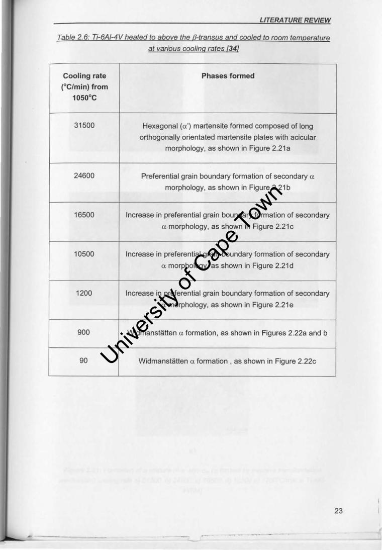
Table 2.6: Ti-6AI-4V heated to above the fUransus and cooled to room temperature
at various cooling rates 1341
Cooling rate Phases formed
(Oe/min) from
1050'C
31500 Hexagonal (a') martensite formed composed of long
orthogonally orientated martensite plates with acicular
morphology, as shown in Figure 2.21a
24600 Preferential grain boundary formation of secondary a
morphology. as shown in Figure 2.21b
16500 Increase in preferential grain boundary formation of secondary
a morphology, as shown in Figure 2.21c
10500 Increase in preferential grain boundary formation of secondary
a morphology, as shown in Figure 2.21d
1200 Increase in preferential grain boundary formation of secondary
a morphology, as shown in Figure 2.21e
900 Widmanstatten a formation, as shown in Figures 2.22a and b
90 Widmanstatlen a formation , as shown in Figure 2.22c
-- - -
23
Univers
ity of
Cap
e Tow
n
LITERA TURE REVIEW
• •
100 ilm
a) b)
a'
0)
Figure 2.21: Formation of a mixture of a ' and am (a formed by massive transformation
mechanism) cooling rate a) 31500, b) 24600, c) 16500, d) 10500 e) 12rxfClmin in Ti·6Af-
4V{34}
.- .... - ---
24
Univers
ity of
Cap
e Tow
n
LITERA TURE REVIEW
, •
a) b)
• ,
• •
,
20 p..m
c)
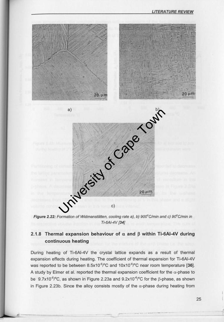
Figure 2.22: Formation of Widmanstatten, cooling rate a), b) 90d'C/min and c) 9cfC/min in
Ti-6AI-4V [34]
2.1.8 Thermal expansion behaviour of a and p within Ti·6AI·4V during
continuous heating
During heating of Ti-6AI-4V the crystal lattice expands as a result of thermal
expansion effects during heating. The coefficient of thermal expansion for Ti-6AI-4V
was reported to be between 8.5x10⁻⁶rC and 10x10-6rC near room temperature [36].
A study by Elmer et al. reported the thermal expansion coefficient for the a -phase to
be 9. 7x1 o-6rc, as shown in Figure 2.23a and 9.2x10⁻⁶fC for the f\-phase, as shown
in Figure 2.23b. Since the alloy consists mostly of the a-phase during heating from
--- -
25
Univers
ity of
Cap
e Tow
n
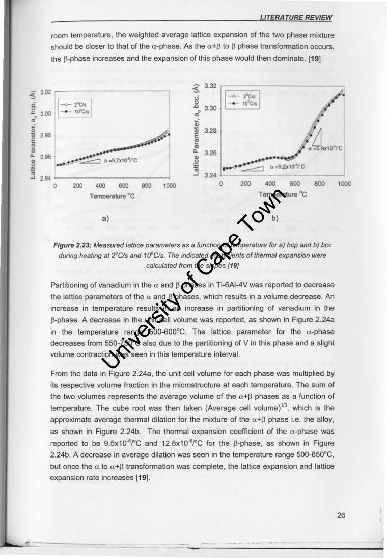
LITERA TURE REVIEW
room temperature, the weighted average lattice expansion of the two phase mixture
should be closer to that of the a -phase. As the a+j3 to j3 phase transformation occurs,
the j3-phase increases and the expansion of this phase would then dominate. [19]
~ 302 -----------
~ 300 I--~· .' ~ 298 E e • ..
2.96 • __ .-II~ tJ. .r9.71C10'rC
" " ~ 3.28
l'! t1. 3.26 8 .--' .~ ~
~ 2.94 -----------
'" _~ ... .2>< 'O.,c ~ I~::-=-----====~~~~~----" 3.24 I-
o 200 400 600 BOO 1000 o 200 400 600 800 1000
Temoeralure °c Temperature °c
a) b)
Figure 2.23: Measured lattice parameters as a function of temperature for a) hcp and b) bee
during heating at ~C/s and ufC/s. The indicated coefficients of thermal expansion were
calculated from the slopes [19J
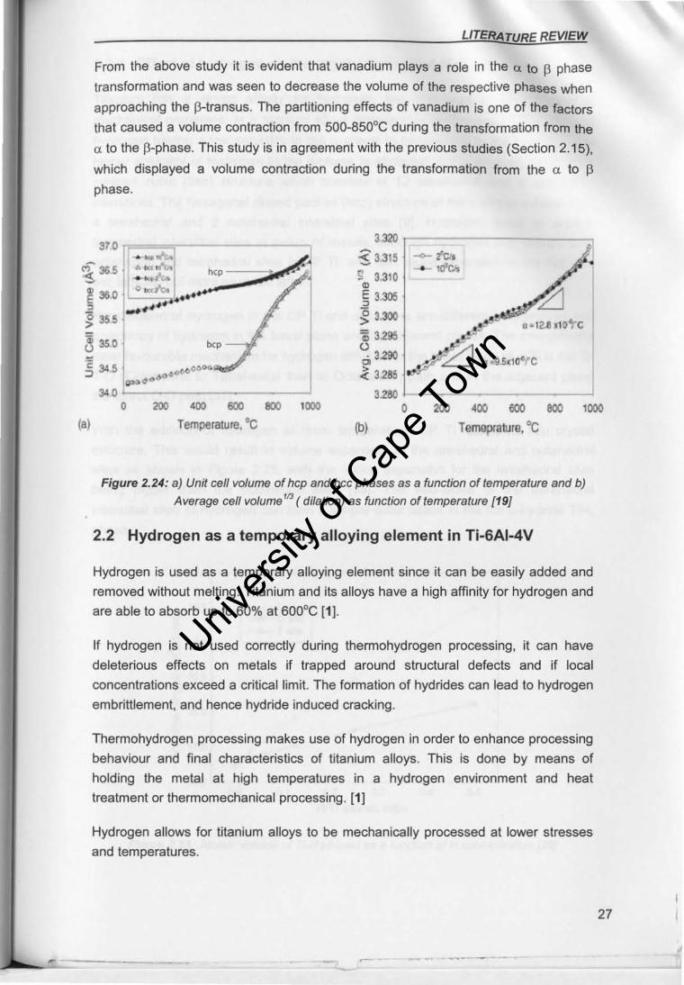
Partitioning of vanadium in the a and p phases in Ti-6AI-4V was reported to decrease
the lattice parameters of the a and p phases, which results in a volume decrease. An
increase in temperature results in an increase in partitioning of vanadium in the
J3-phase. A decrease in the unit cell volume was reported, as shown in Figure 2.24a
in the temperature range 500-600°C. The lattice parameter for the a.-phase
decreases from 550-750oC also due to the partitioning of V in this phase and a slight
volume contraction was seen in this temperature interval.
From the data in Figure 2.24a, the unit cell volume for each phase was multiplied by
its respective volume fraction in the microstructure at each temperature. The sum of
the two volumes represents the average volume of the cx+f3 phases as a function of
temperature. The cube root was then taken (Average cell volume)ll3, which is the
approximate average thermal dilation for the mixture of the a+p phase i.e. the alloy,
as shown in Figure 2.24b. The thermal expansion coefficient of the a-phase was
reported to be 9.5x10⁻⁶rC and 12.8x10⁻⁶fC for the J3-phase, as shown in Figure
2.24b. A decrease in average dilation was seen in the temperature range 500-850oC,
but once the a to a+f3 transformation was complete, the lattice expansion and lattice
expansion rate increases [19].
--- -
26
Univers
ity of
Cap
e Tow
n
LITERA TURE REVIEW
From the above study it is evident that vanadium plays a role in the Cl to j3 phase
transformation and was seen to decrease the volume of the respective phases when
approaching the (3-transus. The partitioning effects of vanadium is one of the factors
that caused a volume contraction from 50Q·850oC during the transformation from the
ex. to the j3-phase. This study is in agreement with the previous studies (Section 2.15),
which displayed a volume contraction during the transformation from the a to j3
phase.
370 3.320
~
~-""" A ~ 3.315 -fcio - tllII.t""'J he - .cfcI. ~ 36S ....... ,.(;10 P ~ 3.3'0 - IO keto. ......... ~
~ 360 .... ~ 3,))5 , .. ~~ ... g 3.300 ~ 355 0·12.8 l'10"rC
B $ .0 ~ 3.295 0
'2 345 . 3.290
(J .. u,tl04r c a O(~ooo.a. ~ 3.285 :::>
g:JQolt06oo
340 3280 0 200 400 600 800 .000 0 200 400 600 600 '000
(8) Temperature. oC (b) Temop!alur • • 'C
Figure 2.24: a) Unit cell volume of hcp and bcc phases as a function of temperature and b)
Average celf volume '13 (dilation) as function of temperature (19)
2.2 Hydrogen as a temporary alloying element in Ti-6AI-4V
Hydrogen is used as a temporary alloying element since it can be easily added and
removed without melting . Titanium and its alloys have a high affinity for hydrogen and
are able to absorb up to 60% at 600' C [1).
If hydrogen is not used correctly during thermohydrogen processing, it can have
deleterious effects on metals if trapped around structural defects and if local
concentrations exceed a critical limit. The formation of hydrides can lead to hydrogen
embrittlement, and hence hydride induced cracking.
Thermohydrogen processing makes use of hydrogen in order to enhance processing
behaviour and final characteristics of titanium alloys. This is done by means of
holding the metal at high temperatures in a hydrogen environment and heat
treatment or thermomechanical processing. {1J
Hydrogen allows for titanium alloys to be mechanically processed at lower stresses
and temperatures.
- -- - ~
27
Univers
ity of
Cap
e Tow
n
LITERATURE REVIEW
2.2.1 Effect of hydrogen on the crystal lattices of titanium alloys
Titanium has a strong affinity for hydrogen, but may lead to deterioration of
mechanical properties. In a titanium alloys hydrogen embrittlement is as a result of
hydrogen having a low solubility in the a phase in comparison to the 13 phase. The
higher solubility of hydrogen in the p-phase is attributed to the relatively open body
centred cubic (bee) structure which consists of 12 tetrahedral and 6 octahedral
interstices. The hexagonal closed packed (hcp) structure of the a phase exhibits only
4 tetrahedral and 2 octahedral interstitial sites (9). Hydrogen tends to occupy
tetrahedral interstitial sites in group IV metals, although hydrogen can occupy both
octahedral and tetrahedral sites in CP Ti and can cause expansion in the hcp and
bcc lattices, but more so in the latter.
For diffusion of hydrogen in the CP Ti unit cell, there are different mechanisms and
anisotropy of hydrogen in the basal plane and the adjacent planes. The energetically
most favourable mechanism for hydrogen diffusion in the basal plane of a-Ti is the 0-
T-O (Octahedral to Tetrahedral then to Octahedral ) path and in the adjacent plane
the direct 0·0 path [37J.
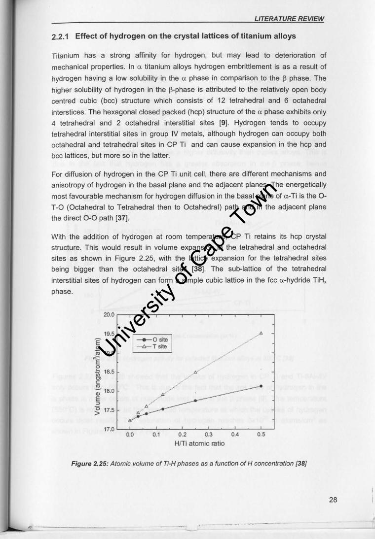
With the addition of hydrogen at room temperature, CP Ti retains its hcp crystal
structure. This would result in volume expansion in the tetrahedral and octahedral
sites as shown in Figure 2.25, with the lattice expansion for the tetrahedral sites
being bigger than the octahedral sites [38] . The sub-lattice of the tetrahedral
interstitial sites of hydrogen can form a simple cubic lattice in the fcc ex-hydride TiH~
phase.
20.0
19.5 • I =:=~ :::
" - " E .9 /
19.0 .
~ "' .• <' .-E ./ 0 ~ 18.5 .-e ~// .... ~ -; 18.0 ,.-E
A "'~ ~
" 17.5 .~~ ........ > r 17.0
0.0 0.1 02 0.3 0.4 0.5
Hm atomic ratio
Figure 2.25: Atomic volume of Ti-H phases as a function of H concentration [38]
---- --- -
28
Univers
ity of
Cap
e Tow
n
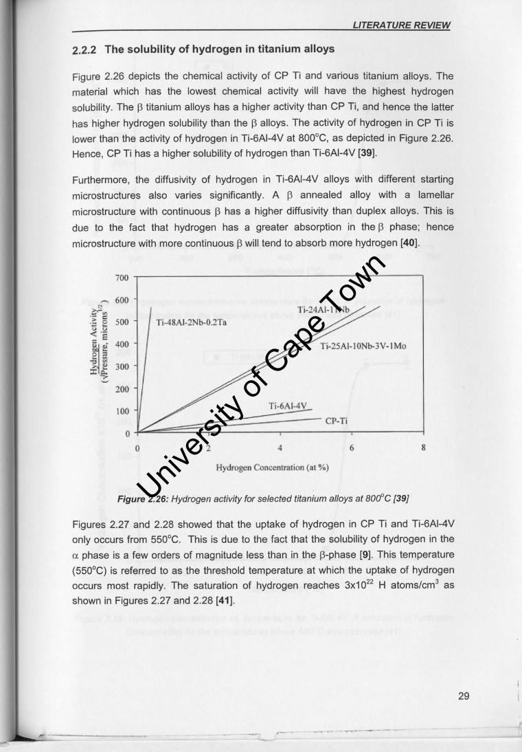
LITERA TURE REVIEW
2.2.2 The solubility of hydrogen in titanium alloys
Figure 2.26 depicts the chemical activity of CP Ti and various titanium alloys. The
material which has the lowest chemical activity will have the highest hydrogen
solubility. The ~ titanium alloys has a higher activity than CP Ti, and hence the latter
has higher hydrogen solubility than the rJ alloys. The activity of hydrogen in CP Ti is
lower than the activity of hydrogen in Ti-6AI-4V at BOQoe, as depicted in Figure 2.26.
Hence. CP Ti has a higher solubility of hydrogen than Ti-6AI-4V [39].
Furthermore, the diffusivity of hydrogen in Ti-6AI-4V alloys with different starting
microstructures also varies significantly. A [3 annealed alloy with a lamellar
microstructure with continuous 13 has a higher diffusivity than duplex alloys. This is
due to the fact that hydrogen has a greater absorption in the p phase; hence
microstructure with more continuous f3 will tend to absorb more hydrogen [40).
700
- 600 ,(,i-24Al-1INb
_ 0
""'-.- . . ~ e 500 Ti-48AI-2Nb-O.2Tn ~ ,~
~~ 400 e a ~ ~ 300 :r~
n~25Al-l ONb-3 V-I Mo
- 200
100 Tj·6AI·4V
CP·Ti
0
0 2 4 6 8
Hydrogen Concentration (a.t %)
Figure 2.26: Hydrogen activity for sefected titanium afloys at 80Cfc [39J
Figures 2.27 and 2.28 showed that the uptake of hydrogen in CP Ti and Ti-6AI-4V
only occurs from 550°C. This is due to the fact that the solubility of hydrogen in the
a phase is a few orders of magnitude less than in the f3-phase [9]. This temperature
(550°C) is referred to as the threshold temperature at which the uptake of hydrogen
occurs most rapidly. The saturation of hydrogen reaches 3x10²² H atoms/cm3 as
shown in Figures 2.27 and 2.28 [41 ].
--- - ----
29
Univers
ity of
Cap
e Tow
n
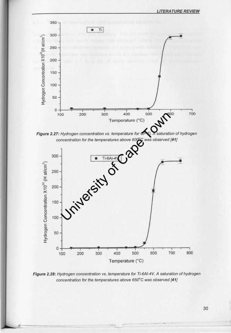
LITERA TURE REVIEW
350
"- 300 E g '" 250 :I:
0.;-X 200 c g I!! 150 C 1l c 0
U 100 c
" 8' ~ 50
:I:
0 100 200 300 400 500 600 700
Temperature (· C)
Figure 2.27: Hydrogen concentration vs. temperature for CP Ti. A saturation of hydrogen concentration for the temperatures above SO<fC was obs8IVed [41]
300 • To-6AI-4V I -" E .g 250 .. J: -~ 0 200 ~
x c g
150 ~ '2 i'l c 100 0
(.) c ., g> 50 ~
." >. J:
0 100 200 300 400 500 600 700 800
Temperature (OC)
Figure 2.28: Hydrogen concentration vs. temperature for Ti-6AI-4V. A saturation of hydrogen
concentration for the temperatures above 65(fC was observed {41]
~- - --30
Univers
ity of
Cap
e Tow
n
LITERATURE REVIEW
2.2.3 Types of thermohydrogen processing treatments
Ti-6AI-4V displays an allotropic behaviour. This will allow for phase transformations
within the alloy, and hence various heat treatment options. Phase transformations
can promote grain refinement however, the grain growth kinetics in Ti-6AI-4V is high
in Ti-6AI-4V. Hydrogen can therefore act as a f3 stabiliser and lowers the f3-transus
temperature. Table 2.7 is a list of some common types of thermohydrogen
processing.
31
Univers
ity of
Cap
e Tow
n
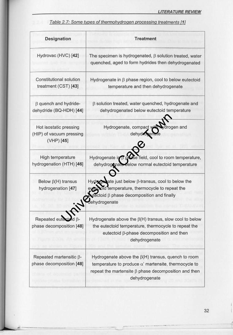
LITERA TURE REVIEW
Table 2.7: Some types of thermo hydrogen processing treatments [11
Designation Treatment
Hydrovac (HVC) [42) The specimen is hydrogenated, J3 solution treated , water
quenched, aged to form hydrides then dehydrogenated
Constitutional solution Hydrogenate in J3 phase region, cool to below eutectoid
treatment (CST) [43) temperature and then dehydrogenate
J3 quench and hydride- J3 solution treated, water quenched, hydrogenate and
dehydride (BQ-HDH) [44) dehydrogenated below eutectoid temperature
Hot isostatic pressing Hydrogenate, compact with hydrogen and
(HIP) of vacuum pressing dehydrogenate
(VHP) [45)
High temperature Hydrogenate in J3 phase field, cool to room temperature,
hydrogenation (HTH) [46) dehydrogenate below normal eutectoid temperature
Below P(H) transus Hydrogenate just below ~-transus, cool to below the
hydrogenation [47) eutectoid temperature, thermocycle to repeat the
eutectoid 13 phase decomposition and finally
dehydrogenate
Repeated eutectoid 13- Hydrogenate above the j3(H) transus, slow cool to below
phase decomposition [48] the eutectoid temperature, thermocycle to repeat the
eutectoid j3-phase decomposition and then
dehydrogenate
Repeated martensitic [3- Hydrogenate above the f3( H) transus, quench to room
phase decomposition [48] temperature to produce a' martensite, thermocycle to
repeat the martensite j3 phase decomposition and then
dehydrogenate
32
--- --
Univers
ity of
Cap
e Tow
n
LITERATURE REVIEW
2.2.4 Principles of thermohydrogen processing
The addition of hydrogen in Ti-6AI-4V is capable of destabilising the low temperature
a-phase and stabilising the more ductile high temperature l3-phase. Due to this the a
phase transforms partly into the l3-phase above the eutectoid temperature.
Furthermore, the temperature of transforming the a-phase to the l3-phase phase is
lowered and the temperature interval of the two phase (a+l3) is increased when
hydrogen is added.
The decrease in the temperature range of the a+13 to 13 transformation (modified 13
transus) due to hydrogen addition leads to reduction in grain growth on heating into
the modified 13 range. The hydrogen-induced increase in the temperature interval of
the a+13 range allows heat treatments to be performed, which would not otherwise
have been possible without hydrogen addition [1]. This in turn leads to different
microstructures in the conventional Ti-6AI-4V alloy and the opportunity to promote
grain refinement in a manner similar to the practice of normalising steels.
2.2.5 Phase transformations within Ti-SAI-4V during hydrogenation
Phase diagrams were proposed by Kerr et al. [28] and lIyin et al. [27], which
displayed significant differences as shown in Figure 2.29. In Figure 2.29a, a hydride
phase formation was proposed by eutectoid transformation of the l3-phase near
800°C. However, in Figure 2.29b, a phase diagram was proposed, which showed a
hydride phase formation present only below 300°C and a wide a+13 phase field above
300°C.
In a study by Qazi et al. cast Ti-6AI-4V was hydrogenated at 780°C and held
isothermally for 24 hours by introducing varying levels of hydrogen within the alloy
i.e. 10, 20, 30 at% H. This was done in order to establish the correct Ti-6AI-4V-H
phase diagram.
Prior to hydrogenation a coarse a+13 lamellar phase with an average prior grain size
of 0.97mm and an average interlamellar a spacing of 5/lm was observed, as shown
in Figure 2.30a. An addition of 10at% H lead to the formation of a and martensite
(a'), as shown in Figure 2.30b and the lamellar space decreased. The martensite
regions were identified as a smooth etch resistant regions between a lamellae. The
martensite volume fraction also increased from 30 to 80 vol%, as the hydrogen
concentration increased from 10 to 30at%. The transformation of a-lamellae into fine
chains of equiaxed particles was observed, as shown in Figures 2.30c and d. A
hydride phase formation was detected in the specimens containing 20 and 30at% H,
but not in the specimen containing 10at%H [6].
33
Univers
ity of
Cap
e Tow
n
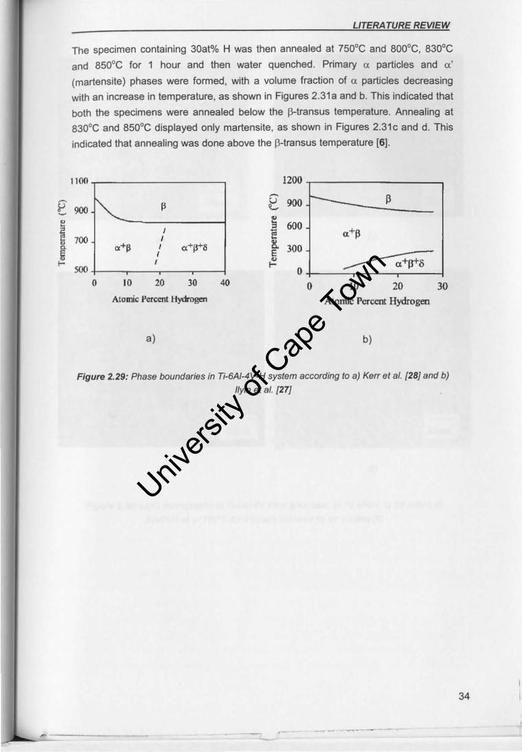
P' -u " ~ ~ ....
LITERATURE REVIEW
The specimen containing 30at% H was then annealed at 750°C and BOQoe, 830°C
and 850°C for 1 hour and then water quenched. Primary a particles and a'
(martensite) phases were formed, with a volume fraction of a particles decreasing
with an increase in temperature, as shown in Figures 2.31a and b. This indicated that
both the specimens were annealed below the J3-transus temperature. Annealing at
830°C and 850°C displayed only martensite, as shown in Figures 2.31c and d. This
indicated that annealing was done above the JHransus temperature (6].
1100 1200
-900 p l::. 900
u ~ 600 il I m a+~
700 I ~
.+p I a+p+ll 8. 300 I E
~ I u .... 500 0
0 10 20 30 40 0 10 20 30 AtOmlC Vereent Hydrogen AtonUc Percent Hydrogen
a) b)
Figure 2.29: Phase boundaries in Ti-6AI-4V-H system according to a) Ke" at 81. (2S] and b)
I/yin et al. {27]
34
Univers
ity of
Cap
e Tow
n
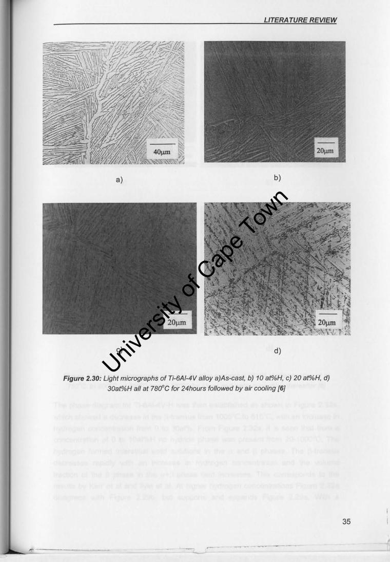
LITERATURE REVIEW
a) b)
c) d)
Figure 2.30: Light micrographs of Ti-6AI-4V alloy a)As--cast, b) 10 afO/oH, c) 20 at%H, d)
30a~!fJH all at 78CfC for 24hours followed by air cooling {6]
--- --35
Univers
ity of
Cap
e Tow
n
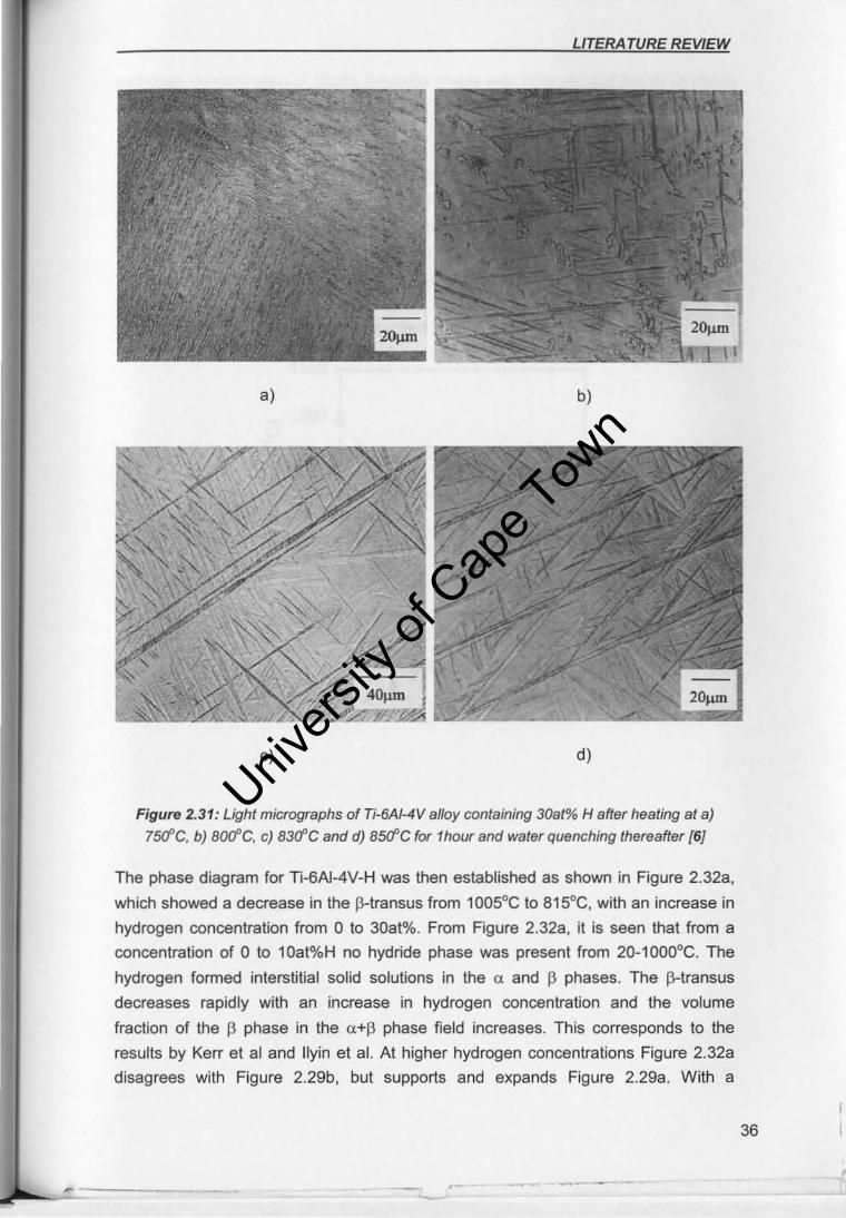
LITERA TURE REVIEW
a) b)
c) d)
Figure 2.31: Light micrographs of Ti-6A1-4Valloy containing 30al% H after heating at a)
75ffC, b) 8()(fC. c) 83Cfe and d) 8ScfC for 1hour and waler quenching thereafter [6J
The phase diagram for Ti-6AI-4V-H was then established as shown in Figure 2.32a,
which showed a decrease in the p-transus from 1005°C to 815°C, with an increase in
hydrogen concentration from 0 to 30al%. From Figure 2.32a, it is seen that from a
concentration of 0 to 10at%H no hydride phase was present from 20-1000oC. The
hydrogen formed interstitial solid solutions in the a and J3 phases. The p-tranSU5
decreases rapidly with an increase in hydrogen concentration and the volume
fraction of the J3 phase in the a+J3 phase field increases. This corresponds to the
results by Kerr et al and lIyin et al. At higher hydrogen concentrations Figure 2.32a
disagrees with Figure 2.29b, but supports and expands Figure 2.29a. With a
36
I
Univers
ity of
Cap
e Tow
n
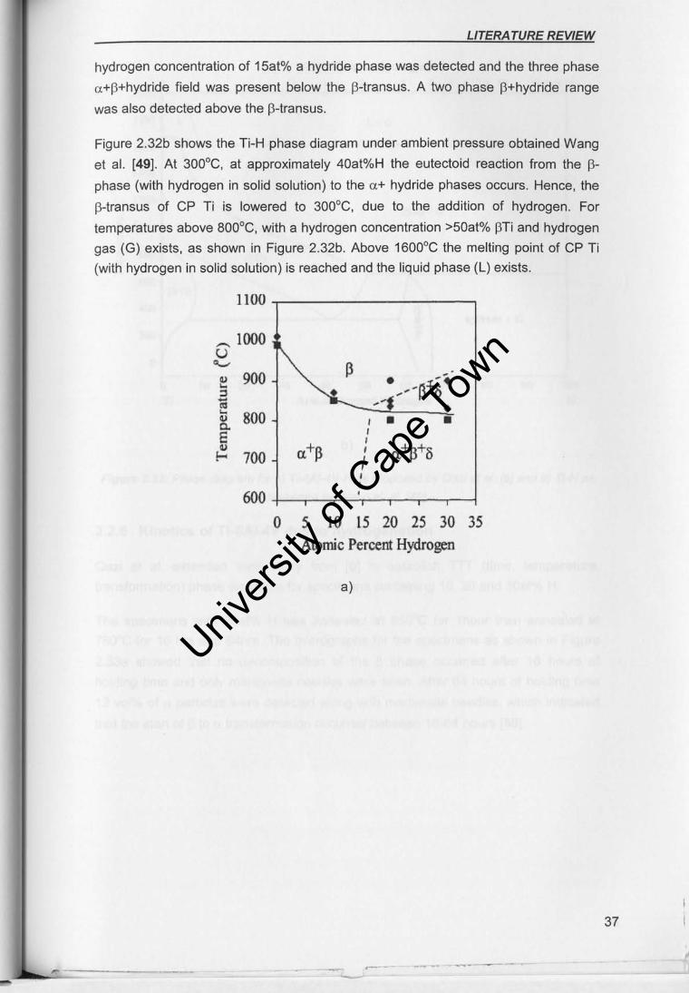
LITERA TURE REVIEW
hydrogen concentration of 15at% a hydride phase was detected and the three phase
a +p+hydride field was present below the f3-transus. A two phase l3+hydride range
was also detected above the f3-transus.
Figure 2.32b shows the Ti-H phase diagram under ambient pressure obtained Wang
et al. (49]. At 30QoC, at approximately 40at%H the eutectoid reaction from the 13-phase (with hydrogen in solid solution) to the a+ hydride phases occurs. Hence, the
fHransus of CP Ti is lowered to 300°C, due to the addition of hydrogen. For
temperatures above BOQce, with a hydrogen concentration >508t% I3Ti and hydrogen
gas (G) exists, as shown in Figure 2.32b. Above 1600°C the melting point of CP Ti
(with hydrogen in solid solution) is reached and the liquid phase (L) exists.
1100
~ 1000
~ u ..... ~ 900 • pf'· ~ :J ......... 0 - ."1 • = ~ 800 ~ I • • a. I E I ~ IJ.+~ I 1J.+~+o 1- 700 ,
I , , 600 •
0 5 10 15 20 25 30 35 Atomic Percent Hydrogen
a)
- ~. --- --37
Univers
ity of
Cap
e Tow
n
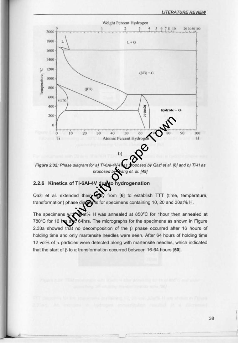
LITERA TURE REVIEW
Weight Percent Ilydroscn l l..1 5 6 78 10 203050100
<PTI)+G
hydJi dc + C
t---~~~~--~~--4~o~-'o~--C~C~~~io~--~80C---~~'~·~I 00 Atomic Percent Hydrogen H
b)
Figure 2.32: Phase diagram for a) Ti-6AI-4V-H as proposed by Qazi et al. (6) and b) Ti-H as
proposed by Wang et. al. [49]
2.2.6 Kinetics of Ti-6AI-4V due to hydrogenation
Qazi et al. extended their study from [6] to establish TIT (time, temperature,
transformation) phase diagrams for specimens containing 10,20 and 30at% H.
The specimens with 30at% H was annealed at 850°C for 1 hour then annealed at
780°C for 16 hrs and 64hrs. The micrographs for the specimens as shown in Figure
2.33a showed that no decomposition of the 13 phase occurred after 16 hours of
holding time and only martensite needles were seen. After 64 hours of holding time
12 vol% of ex particles were detected along with martensite needles. which indicated
that the start of 13 to ex transformation occurred between 16-64 hours [50).
---
38
Univers
ity of
Cap
e Tow
n
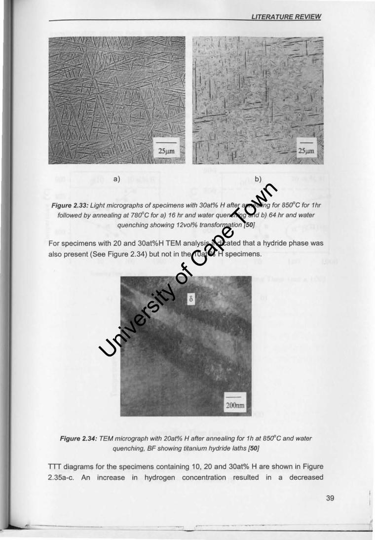
a)
I I • I
LITERA TURE REVIEW
b)
Figure 2.33: Ught micrographs of specimens with 30al% H after annealing for 8Sa"C for 1hr
followed by annealing at 78(/'C for a) 16 hr and water quenching and b) 64 hr and water
quenching showing 12vo/% transformation {50]
For specimens with 20 and 30at%H TEM analysis indicated that a hydride phase was
also present (See Figure 2.34) but not in the 10at % H specimens.
Figure 2.34: rEM micrograph with 208t% H after annealing for 1h at 85Cfc and water
quenching, BF showing titanium hydride laths [SO}
TTT diagrams for the specimens containing 10, 20 and 30at% H are shown in Figure
2.35a-c. An increase in hydrogen concentration resulted in a decreased
39
Univers
ity of
Cap
e Tow
n
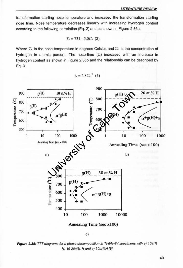
LITERA TURE REVIEW
transformation starting nose temperature and increased the transformation starting
nose time. Nose temperature decreases linearly with increasing hydrogen content
according to the following correlation (Eq. 2) and as shown in Figure 2.36a.
T. = 73 1- S.Oc" (2),
Where TN is the nose temperature in degrees Celsius and eN is the concentration of
hydrogen in atomic percent. The nose-time (~) increased with an increase in
hydrogen content as shown in Figure 2.36b and the relationship can be described by
Eq. 3.
/. = 2.8e. 2 (3)
900 ~ __________ ~ ____ __ 20at.% H 900 p(H) lOat% H
: ~~(H) ~ 800 • • E 800
" :a 700
SR 600 ~
p(H)+o
p(H) • •
5oo+----r--~--~ •• 500+-____ ~----~--~
10 100 1000 10 100 1000
Annealing Time (sec 1100) Annealing Time (sec x 100)
a) b)
900
~ 800 u 'L- 700 "
n(H) 30 al.% H __ _ l:!. _ _ __ __ __ _
---"~. ~
" 10 600 ~
" 0-S 500 " f-
400 10 100 1000 10000
Annealing Time (sec x l 00)
c)
Figure 2.35: TTT diagrams for b phase decomposition in Ti-6AI-4V specimens with a) 1OafCA,
H, b) 20at% H and c) 30at%H {61
40
Univers
ity of
Cap
e Tow
n
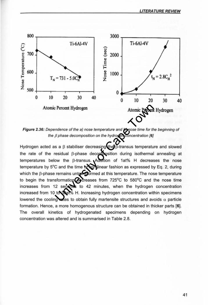
LITERA TURE REVIEW
goo 3000 ~ T~6Al-4V Ti-6Al-4V Y ~
'- ~ e 700 ~ 2000 ~
" ~ ~
~ E -Q i= 0-E 600 ~ 1000 ~ ~
tN = 2.8CH' i-- TN =731-5.OCH 0
• Z • 0 Z 500 0
0 10 20 30 40 0 10 20 30 40 Atomic Percent Hydrogen Atomic Percent Hydrogen
Figure 2.36: Dependence of the a) nose temperature and b) nose time for the beginning of
the p phase decomposition on the hydrogen concentration (6)
Hydrogen acted as a f3 stabiliser decreasing the p-transus temperature and slowed
the rate of the residual (3-phase decomposition during isothennal annealing at
temperatures below the ~transus. Addition of 1al% H decreases the nose
temperature by 5°C and the time in non linear fashion as expressed by Eq. 2. during
which the p-phase remains untransformed at this temperature. The nose temperature
to begin the transformation decreases from 725°C to 58Doe and the nose time
increases from 12 seconds to 42 minutes, when the hydrogen concentration
increased from 10 to 30at% H. Increasing hydrogen concentration within specimens
lowered the cooling rates to obtain fully martensite structures and avoids a particle
formation . Hence, a more homogenous structure can be obtained in thicker parts [6].
The overall kinetics of hydrogenated specimens depending on hydrogen
concentration was altered and is summarised in Table 2.8.
41
Univers
ity of
Cap
e Tow
n
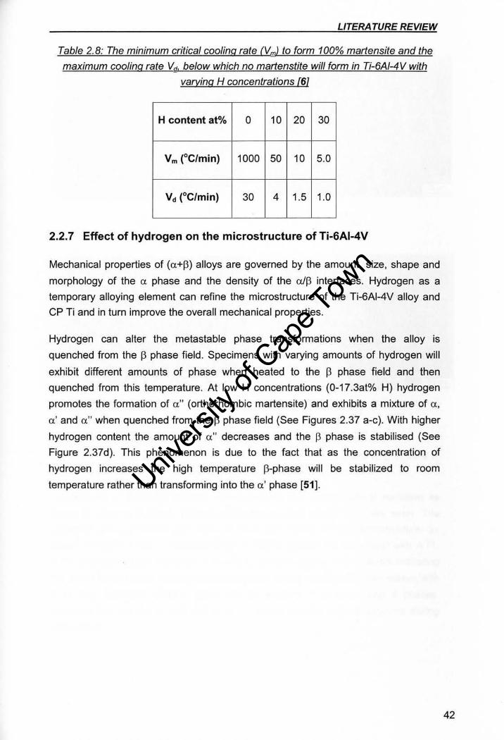
LITERA TURE REVIEW
Table 2.8: The minimum critical cooling rate (V ml to form 100% martensite and the
maximum cooling rate Va. below which no martenstite will form in Ti-6AI-4 V with
varying H concentrations l61
H content at% 0 10 20 30
Vm (DC/min) 1000 50 10 5.0
V, (' C/min) 30 4 1.5 1.0
2.2.7 Effect of hydrogen on the microstructure of Ti-6AI-4V
Mechanical properties of (a+p) alloys are governed by the amount, size, shape and
morphology of the ex. phase and the density of the alP interfaces. Hydrogen as a
temporary alloying element can refine the microstructure of the Ti-6AI-4V alloy and
CP Ti and in turn improve the overall mechanical properties.
Hydrogen can alter the metastable phase transformations when the alloy is
quenched from the 13 phase field . Specimens with varying amounts of hydrogen will
exhibit different amounts of phase when heated to the B phase field and then
quenched from this temperature. At low H concentrations (0-17.3at% H) hydrogen
promotes the formation of a" (orthorhombic martensite) and exhibits a mixture of a,
a' and a" when quenched from the p phase field (See Figures 2.37 a-c). With higher
hydrogen content the amount of a" decreases and the B phase is stabilised (See
Figure 2.37d). This phenomenon is due to the fact that as the concentration of
hydrogen increases the high temperature rJ-phase will be stabilized to room
temperature rather than transforming into the a ' phase [51].
42
Univers
ity of
Cap
e Tow
n
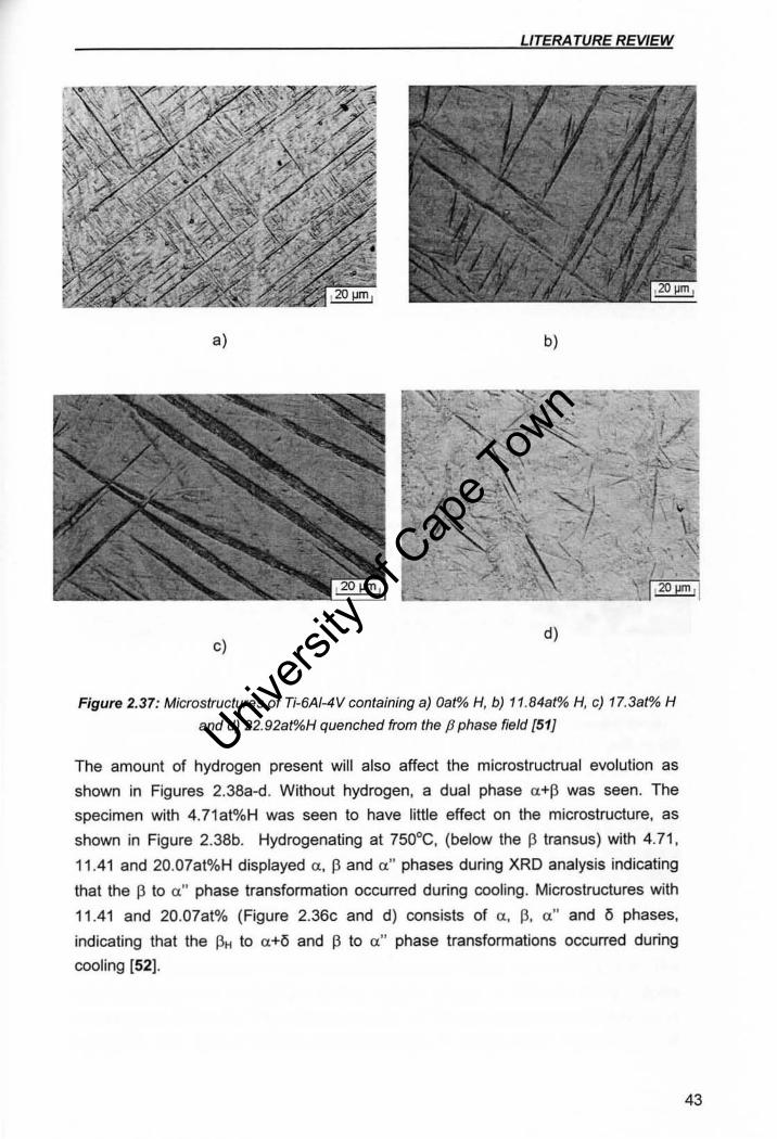
LITERATURE REVIEW
a) b)
, ,-') -
t... ___ ..;.,;,;;. _____ ' .. ' ,20 pm 'I
c) d)
Figure 2.37: Microstructures of Ti-6AI-4V containing a) 081% H, b) 11.848W" H, c) 17.3at% H
and d) 22. 92at%H quenched from the p phase field [51J
The amount of hydrogen present will also affect the microstructrual evolution as
shown in Figures 2.38a-d. Without hydrogen, a dual phase a+f3 was seen. The
specimen with 4.71at%H was seen to have little effect on the microstructure, as
shown in Figure 2.38b. Hydrogenating at 750°C, (below the p transus) with 4.71,
11.41 and 20.07at%H displayed a, Jl and a" phases during XRD analysis indicating
that the j3 to a" phase transformation occurred during cooling. Microstructures with
11.41 and 20.07al% (Figure 2.36c and d) consists of 0 , 13. a" and lj phases,
indicating that the I3H to a+o and 13 to a" phase transformations occurred during
cooling [52).
43
Univers
ity of
Cap
e Tow
n
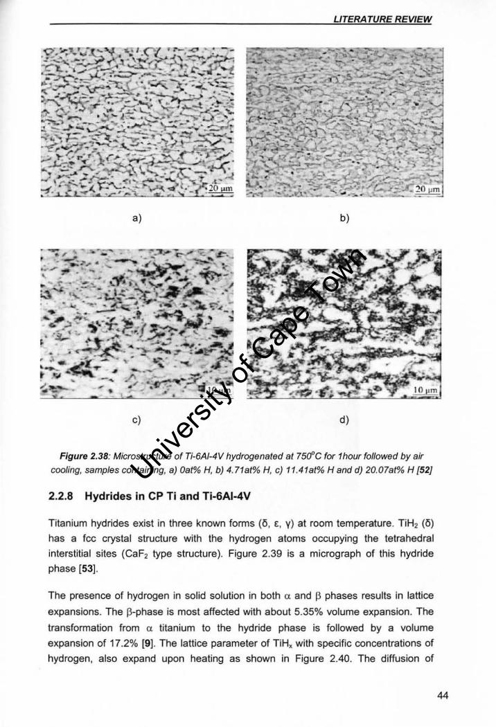
LITERA TURE REVIEW
a) b)
c) d)
Figure 2.38: Microstructure of Ti-6AI-4V hydrogenated at 7sCfc for 1hour followed by air
coofing, samples containing, a) Oa~" H, b) 4. 71al% H. c) 11.41afOA, H and d) 20.07a«l/o H [52J
2.2.8 Hydrides in CP Ti and Ti-6AI-4V
Titanium hydrides exist in three known fanTIs (6, E, y) at room temperature. TiH2 (6)
has a fcc crystal structure with the hydrogen atoms occupying the tetrahedral
interstitial sites (CaF2 type structure). Figure 2.39 is a micrograph of this hydride
phase [53].
The presence of hydrogen in solid solution in both ex and f3 phases results in lattice
expansions. The (3-phase is most affected with about 5.35% volume expansion. The
transformation from ex titanium to the hydride phase is followed by a volume
expansion of 17.2% [9] . The lattice parameter of TiHx with specific concentrations of
hydrogen, also expand upon heating as shown in Figure 2.40. The diffusion of
44
Univers
ity of
Cap
e Tow
n
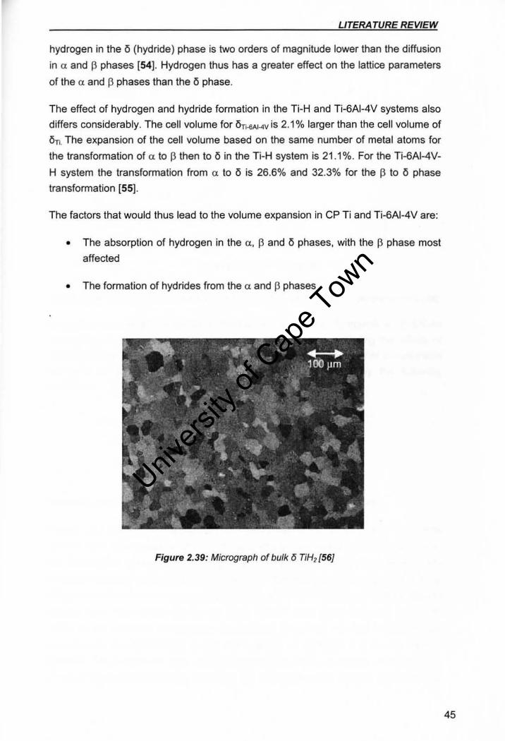
LITERATURE REVIEW
hydrogen in the (5 (hydride) phase is two orders of magnitude lower than the diffusion
in a and p phases [54] . Hydrogen thus has a greater effect on the lattice parameters
of the a and 13 phases than the (5 phase.
The effect of hydrogen and hydride formation in the Ti-H and Ti-6AI-4V systems also
differs considerably. The cell volume for OTl-eAI-4V is 2.1 % larger than the cell volume of
OTt The expansion of the cell volume based on the same number of metal atoms for
the transformation of a to 13 then to (5 in the Ti-H system is 21.1 %. For the Ti-6AI-4V
H system the transformation from a to 0 is 26.6% and 32.3% for the 13 to 0 phase
transformation [551.
The factors that would thus lead to the volume expansion in CP T i and Ti-6AI-4V are:
• The absorption of hydrogen in the a, f3 and 0 phases, with the f3 phase most
affected
• The formation of hydrides from the a and f3 phases
Figure 2.39: Micrograph of bulk 0 TiHzl56]
45
Univers
ity of
Cap
e Tow
n
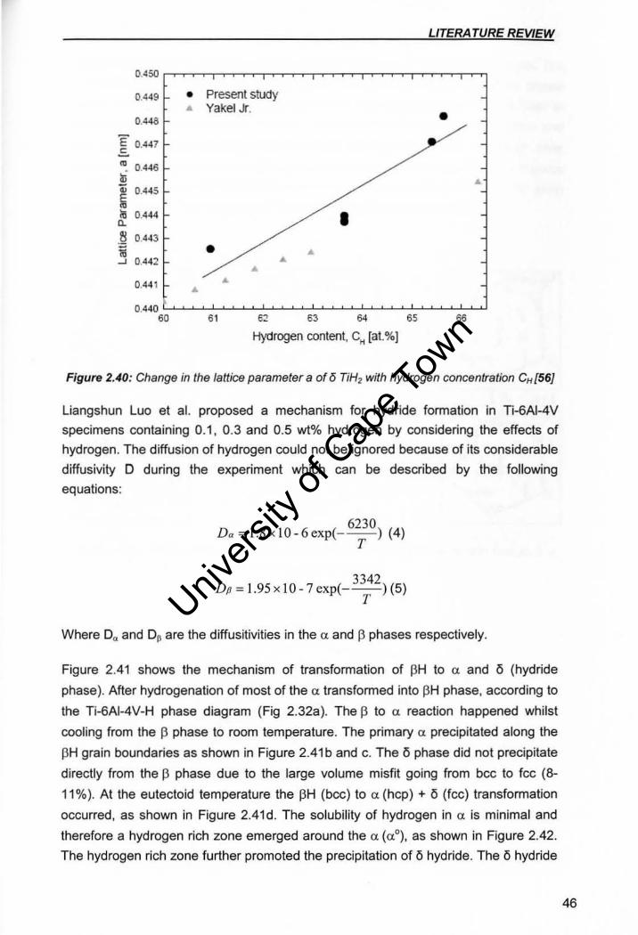
LITERA TURE REVIEW
0.450
0.449 • Present study • Yakel Jr.
0.448 • E E-
0.447
m 0.446 ~ 0; 0.445
~ •
• 0.444 a. • .~ 0.443 ;;; -' 0.442 • • • •
0.441 • • 0.440
60 51 62 63 64 65 .. Hydrogen content, C ... [a1.%)
Figure 2.40: Change in the lattice parameter a of 0 TiH2 with hydrogen concentration CH [56J
Liangshun Luo et a!. proposed a mechanism for hydride formation in Ti-6AI-4V
specimens containing 0.1, 0.3 and 0.5 wt% hydrogen by considering the effects of
hydrogen. The diffusion of hydrogen could not be ignored because of its considerable
diffusivity D during the experiment which can be described by the following
equations:
6230 D. ~ 1.8xI0-6exp(--- ) (4)
T
3342 Dp ~ 1.95 x 10 -7 exp(---) (5)
T
Where Da and Op are the diffusitivities in the a. and 13 phases respectively.
Figure 2.41 shows the mechanism of transformation of I3H to a and l5 (hydride
phase). After hydrogenation of most of the ex transformed into PH phase, according to
the Ti-6AI-4V-H phase diagram (Fig 2.32a). The P to ex reaction happened whilst
cooling from the f3 phase to room temperature. The primary a precipitated along the
PH grain boundaries as shown in Figure 2.41b and c. The l) phase did not precipitate
directly from the P phase due to the large volume misfit going from bcc to fcc (8-
11%). At the eutectoid temperature the PH (bee) to ex (hcp) + l) (fcc) transformation
occurred, as shown in Figure 2.41d. The solubility of hydrogen in ex is minimal and
therefore a hydrogen rich zone emerged around the ex (0.0), as shown in Figure 2.42.
The hydrogen rich zone further promoted the precipitation of l) hydride. The l) hydride
46
Univers
ity of
Cap
e Tow
n
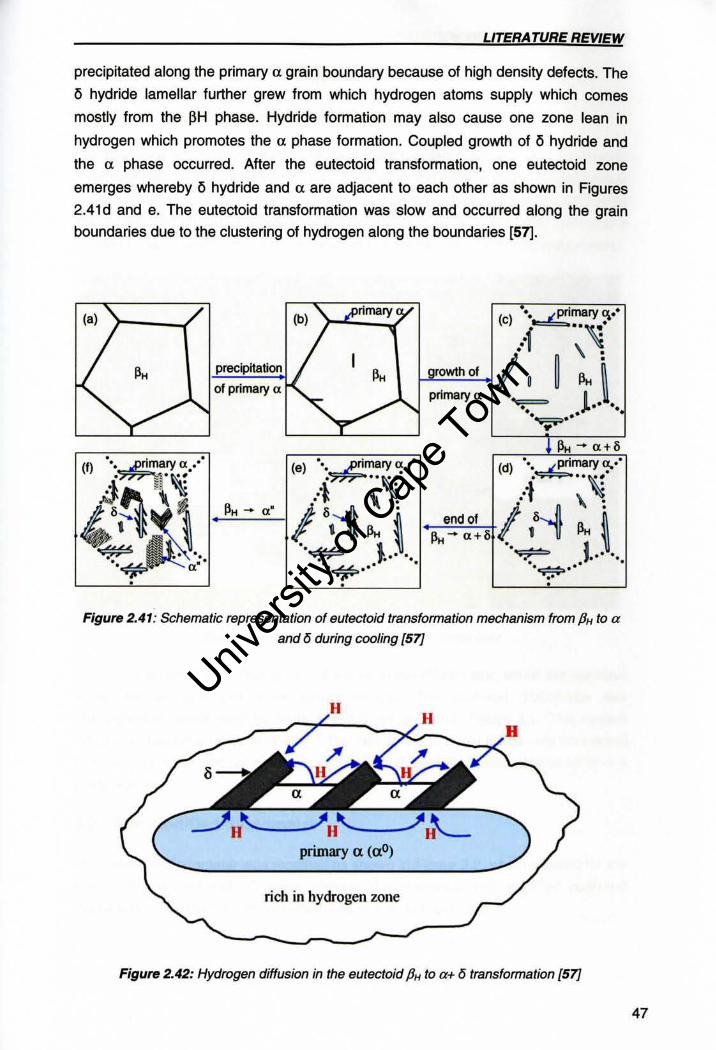
LITERA TURE REVIEW
precipitated along the primary a grain boundary because of high density defects. The
15 hydride lamellar further grew from which hydrogen atoms supply which comes
mostly from the pH phase. Hydride formation may also cause one zone lean in
hydrogen which promotes the a phase formation . Coupled growth of 0 hydride and
the a phase occurred. After the eutectoid transformation, one eutectoid zone
emerges whereby l:i hydride and a are adjacent to each other as shown in Figures
2.41d and B. The eutectoid transformation was slow and occurred along the grain
boundaries due to the clustering of hydrogen along the boundaries [57].
(a) "\. / (b)"\. "Primaoy 'Y (e) ,,~maoy :,'I"
/1 :f .. ~ , \ '
PH precipitation PH I orowth of I . ~ PH~ .......
of primary a
~ "- primary a .. ~ l .. 0. , , .~ ..
• l PH-a+~
(f) oO:;f.!i";!y .~ ... , (e) • •• ~mary~", (d) ',,~maoy ,!-"
~A I\1 :l "~ , "\i :t \ ' PH - a' 1~1i ~ : eodot .( I~i ~ ~ •
~ ~'" "~ l.,t ~- a+8
~ I"", , , . ''¥' a' .. ~ .. , .~.,
" , ,
Figure 2.41: Schematic representation of eutectoid transformation mechanism from PH to a
and 6 during cooling {57}
H
primary a (aO)
rich in hydrogen zone
Figure 2.42: Hydrogen diffusion in the eutectoid PH to a+ 6 transformation {57}
47
Univers
ity of
Cap
e Tow
n
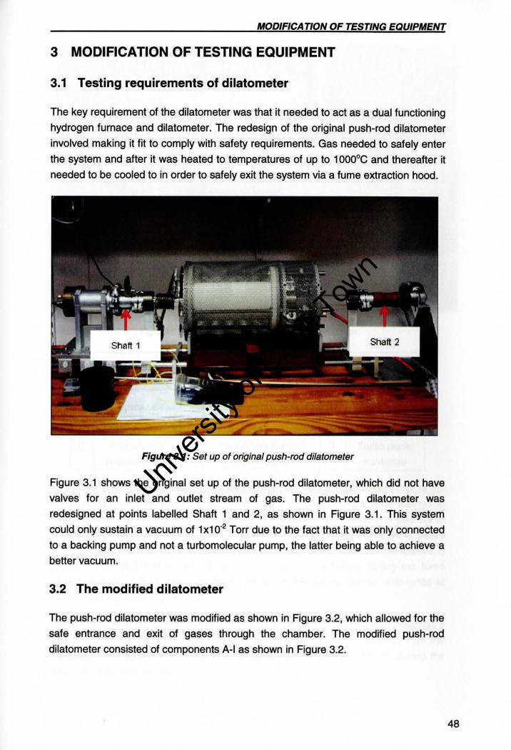
MODIFICATION OF TESTING EQUIPMENT
3 MODIFICATION OF TESTING EQUIPMENT
3.1 Testing requirements of dilatometer
The key requirement of the dilatometer was that it needed to act as a dual functioning
hydrogen furnace and dilatometer. The redesign of the original push-rod dilatometer
involved making it fit to comply with safety requirements. Gas needed to safely enter
the system and after it was heated to temperatures of up to 10000 C and thereafter it
needed to be cooled to in order to safely exit the system via a fume extraction hood.
Figure 3.1: Set up of onginal push-rod dilatometer
Figure 3.1 shows the original set up 01 the push-rod dilatometer, which did not have
valves for an inlet and outlet stream of gas. The push-rod dilatometer was
redesigned at pOints labelled Shaft 1 and 2, as shown in Figure 3.1. This system
could only sustain a vacuum of 1x10·2 Torr due to the fact that it was only connected
to a backing pump and not a turbomolecular pump, the latter being able to achieve a
better vacuum.
3.2 The modified dilatometer
The push-rod dilatometer was modified as shown in Figure 3.2, which allowed for the
safe entrance and exit of gases through the chamber. The modified push-rod
dilatometer consisted of components A-I as shown in Figure 3.2.
48
Univers
ity of
Cap
e Tow
n
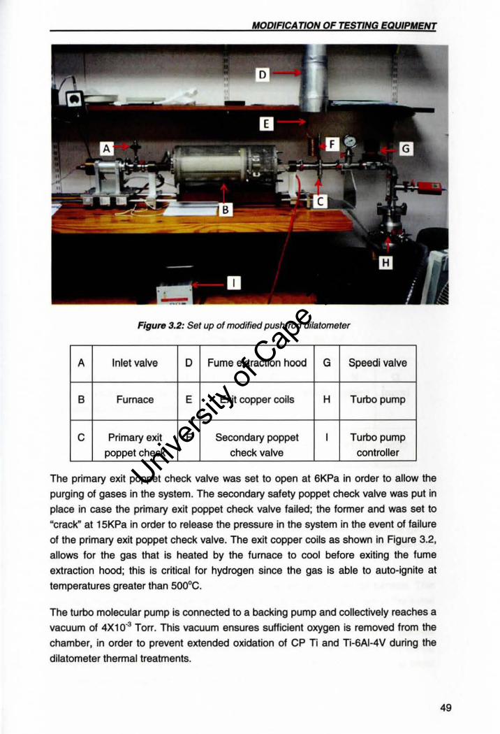
MODIFICATION OF TESTING EQUIPMENT
Figure 3.2: Set up of modified push-rod dilatometer
A Inlet valve D Fume extraction hood G Speedi valve
B Furnace E Exit copper coils H Turbo pump
C Primary exit F Secondary poppet I Turbo pump
poppet check check valve controller
The primary exit poppet check valve was set to open at 6KPa in order to allow the
purging of gases in the system. The secondary safety poppet check valve was put in
place in case the primary exit poppet check valve failed; the former and was set to
"crack" at 15KPa in order to release the pressure in the system in the event of failure
of the primary exit poppet check valve. The exit copper coils as shown in Figure 3.2,
allows for the gas that is heated by the furnace to cool before exiting the fume
extraction hood; this is critical for hydrogen since the gas is able to auto-ignite at
temperatures greater than 500°C.
The turbo molecular pump is connected to a backing pump and collectively reaches a
vacuum of 4X10⁻³ Torr. This vacuum ensures sufficient oxygen is removed from the
chamber, in order to prevent extended oxidation of CP Ti and Ti-6AI-4V during the
dilatometer thermal treatments.
49
Univers
ity of
Cap
e Tow
n
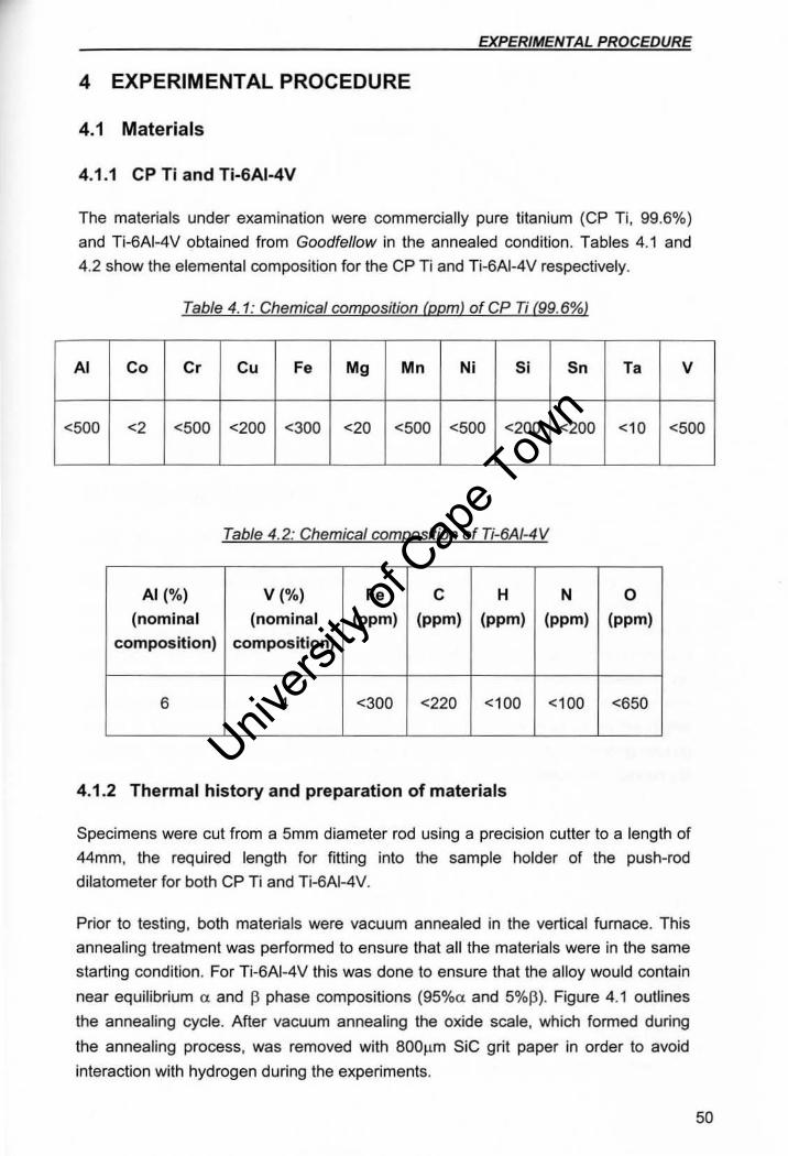
EXPERIMENTAL PROCEDURE
4 EXPERIMENTAL PROCEDURE
4.1 Materials
4.1 .1 CP Ti and Ti-6AI-4V
The materials under examination were commercially pure titanium (CP Ti, 99.6%)
and Ti-6AI-4V obtained from Goodfellow in the annealed condition. Tables 4.1 and
4.2 show the elemental composition for the CP Ti and Ti-6AI-4V respectively.
Table 4. 1: Chemical composition (ppm) of CP Ti (99.6%)
AI Co Cr Cu Fe Mg Mn Ni Si Sn To V
<500 <2 <500 <200 <300 <20 <500 <500 <200 <200 <10 <500
Table 4.2: Chemical composition of Ti-6AI-4V
AI ('!o) V ('!o ) Fe C H N 0 (nominal (nominal (ppm) (ppm) (ppm) (ppm) (ppm)
composition) composition)
6 4 <300 <220 <100 <100 <650
4.1 .2 Thermal history and preparation of materials
Specimens were cut from a 5mm diameter rod using a precision cutter to a length of
44mm, the required length for fitting into the sample holder of the push-rod
dilotometer for both CP Ti and Ti-6AI-4V.
Prior to testing, both materials were vacuum annealed in the vertical furnace . This
annealing treatment was performed to ensure that all the materials were in the same
starting condition. For Ti-6AI-4V this was done to ensure that the alloy would contain
near equilibrium a and p phase compositions (95%a and 5%13). Figure 4.1 outlines
the annealing cycle. After vacuum annealing the oxide scale, which formed during
the annealing process, was removed with 800J.1m SiC grit paper in order to avoid
interaction with hydrogen during the experiments.
50
Univers
ity of
Cap
e Tow
n
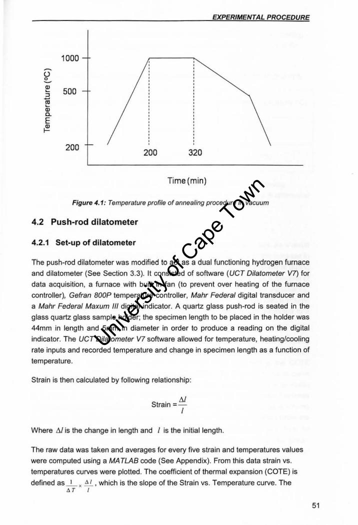
EXPERIMENTAL PROCEOURE
1000 -() 0 -OJ 500 ~
" ~ '" ~ " Co E ~
200 200 320
Time(min)
Figure 4.1: Temperature profile of annealing procedure in vacuum
4.2 Push-rod dilatometer
4.2.1 Set-up of dilatometer
The push-rod dilatometer was modified to act as a dual functioning hydrogen furnace and dilatometer (See Section 3.3). It consisted of software (UeT Dilatometer V7) for
data acquisition. a furnace with built in fan (to prevent over heating of the furnace
controller), Gefran 800P temperature controller, Mahr Federal digital transducer and
a Mahr Federal Maxum 1/1 digital indicator. A quartz glass push-rod is seated in the
glass quartz glass sample holder; the specimen length to be placed in the holder was
44mm in length and Smm in diameter in order to produce a read ing on the digital
indicator. The VCT Dilatometer V7 software allowed for temperature, heating/cooling
rate inputs and recorded temperature and change in specimen length as a function of
temperature.
Strain is then calculated by following relationship :
. t:.I Strain =
I
Where 6/ is the change in length and / is the initial length.
The raw data was taken and averages for every five strain and temperatures values
were computed using a MA TLAB code (See Appendix). From this data strain vs.
temperatures curves were plotted. The coefficient of thermal expansion (COTE) is
defined as _ '_ x ~ ,which is the slope of the Strain vs. Temperature curve. The • r I
51
Univers
ity of
Cap
e Tow
n
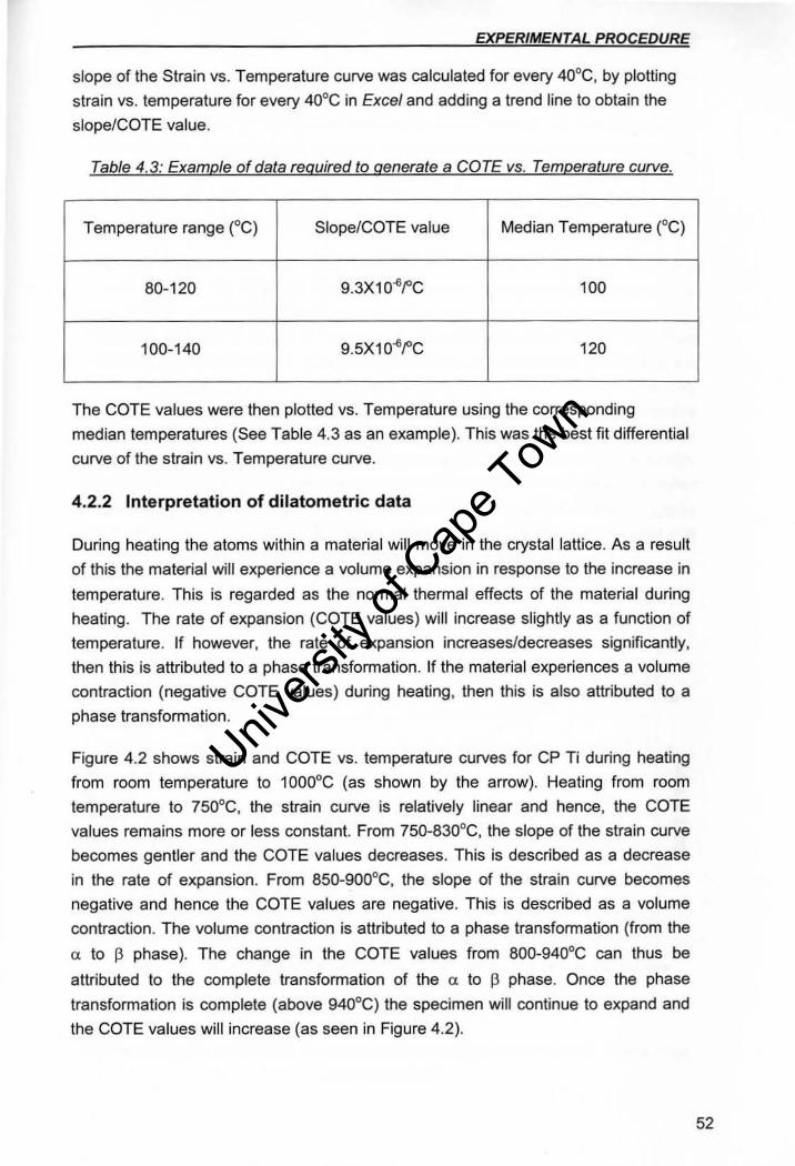
EXPERIMENTAL PROCEDURE
slope of the Strain VS. Temperature curve was calculated for every 40°C. by plotting
strain vs. temperature for every 40°C in Excel and adding a trend line to obtain the
slope/COTE value.
Table 4.3: Example of data required to generate a COTE vs. Temperature curve.
Temperature range (oG) Slope/COTE value Median Temperature (oG)
80-120 9.3XW6i"C 100
100-140 9 . 5X10~i"C 120
The COTE values were then plotted VS. Temperature using the corresponding
median temperatures (See Table 4.3 as an example). This was the best fit differential
curve of the strain vs. Temperature curve.
4.2.2 Interpretation of dilatometric data
During heating the atoms within a material will move in the crystal lattice. As a result
of this the material will experience a volume expansion in response to the increase in
temperature. This is regarded as the normal thermal effects of the material during
heating. The rate of expansion (COTE values) will increase slightly as a function of
temperature. If however. the rate of expansion increases/decreases significantly.
then this is attributed to a phase transformation. If the material experiences a volume
contraction (negative COTE values) during heating. then this is also attributed to a
phase transformation.
Figure 4.2 shows strain and COTE vs. temperature curves for CP Ti during heating
from room temperature to 1000°C (as shown by the arrow). Heating from room
temperature to 750°C. the strain curve is relatively linear and hence. the COTE
values remains more or less constant. From 750-830°C. the slope of the strain curve
becomes gentler and the COTE va lues decreases. This is described as a decrease
in the rate of expansion. From 850-900°C. the slope of the strain curve becomes
negative and hence the COTE values are negative. This is described as a volume
contraction. The volume contraction is attributed to a phase transformation (from the
a to [3 phase). The change in the COTE va lues from 800-940oC can thus be
attributed to the complete transformation of the a to 13 phase. Once the phase
transformation is complete (above 940°C) the specimen will continue to expand and
the COTE va lues will increase (as seen in Figure 4.2).
52
Univers
ity of
Cap
e Tow
n
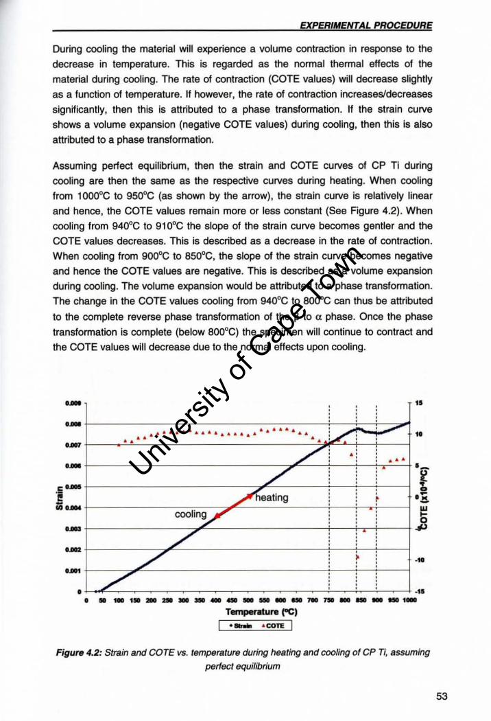
EXPERIMENTAL PROCEDURE
During cooling the material will experience a volume contraction in response to the
decrease in temperature. This is regarded as the normal thermal effects of the
material during cooling. The rate of contraction (COTE values) will decrease slightly
as a function of temperature. If however, the rate of contraction increases/decreases
significantly, then this is attributed to a phase transformation. If the strain curve
shows a volume expansion (negative COTE values) during cooling, then this is also
attributed to a phase transformation.
Assuming perfect equilibrium. then the strain and COTE curves of CP Ti during
cooling are then the same as the respective curves during heating. When cooling
from 100QoC to 950°C (as shown by the arrow), the strain curve is relatively linear
and hence, the COTE values remain more or less constant (See Figure 4.2). When
cooling from 940°C to 910°C the slope of the strain curve becomes gentler and the
COTE values decreases. This is described as a decrease in the rate of contraction.
When cooling from 9000C to esooc, the slope of the strain curve becomes negative
and hence the COTE values are negative. This is described as a volume expansion
during cooling. The volume expansion would be attributed to a phase transformation.
The change in the COTE values cooling from 940°C to BOOoC can thus be attributed
to the complete reverse phase transformation of the p to (l phase. Once the phase
transformation is complete (below BOO°C) the specimen will continue to contract and
the COTE values will decrease due to the normal effects upon cooling.
· · · .. -- • • · · · · · · · -- · · · .. " ...... " .. ............ · • ........ " .. .. ...... " v. · •• • • • • •• ..
/ i · · . : · · ••• · · /' · · · · · · · · · · • • · · ·
..,/'heating • · · · · · · · , • · · · •
COOliY · · · • • • · · · · /' · · • • • · · ·
/' • • , · · • • · ·
./ • • · · · · • · • •
r-..... '-~
·E j
.... _11 ,-
, -,. .. _------------------T.rnper.ture r'CJ I • ..,. .. COTE I
Figure 4.2: Strain and COTE vs. temperature during heating and cooling of CP Ti, assuming
perlect equilibrium
53
Univers
ity of
Cap
e Tow
n
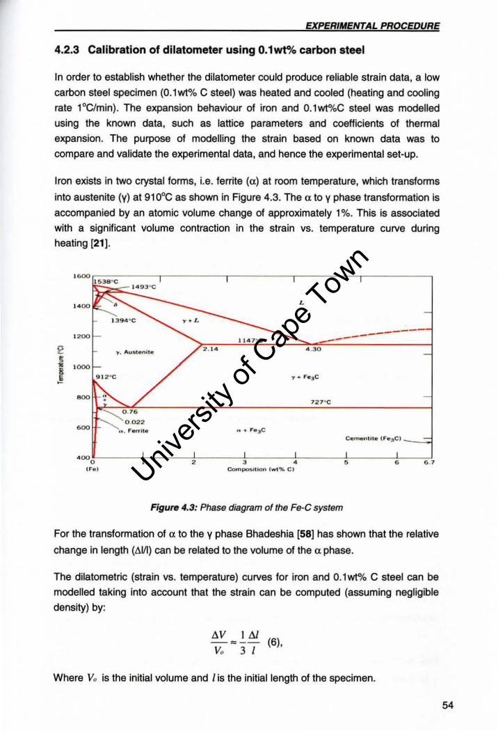
EXPERIMENTAL PROCEOURE
4.2.3 Calibration of dilatometer using O.lwt"lo carbon steel
In order to establish whether the dilatometer could produce reliable strain data, a low
carbon steel specimen (0.1 wt% C steel) was heated and cooled (heating and cooling
rate 1°C/min) . The expansion behaviour of iron and O.1wt%C steel was modelled
using the known data. such as lattice parameters and coefficients of thermal
expansion. The purpose of modelling the strain based on known data was to
compare and validate the experimental data, and hence the experimental set-up.
Iron exists in two crystal forms, i.e. ferrite (a) at room temperature, which transforms
into austenite (V) at 910°C as shown in Figure 4.3. The a to V phase transformation is
accompanied by an atomic volume change of approximately 1 %. This is associated
with a significant volume contraction in the strain vs. temperature curve during
heating (21).
,..,., 1 538 "C
14 93"C
''''" • ----...
' ''''' --------I! l'. "'"sceni le ' .30 ;
j ' 000 9 12 "C
800 727"C
~0.76
0022 600
" . f'" ... h.
' 00" 2 , . , , 6 .' ( f'"el Composition ( wi " CI
Figure 4.3: Phase diagram of the Fe-C system
For the transformation of (X to the V phase Bhadeshia [58) has shown that the relative
change in length (toVl) can be related to the volume of the a phase.
The dilatometric (strain vs. temperature) curves for iron and O.1wt% C steel can be
modelled taking into account that the strain can be computed (assuming negligible
density) by:
toV II!J -=-- (6), V. 3 I
Where Vo is the initial volume and I is the initial length of the specimen.
54
Univers
ity of
Cap
e Tow
n
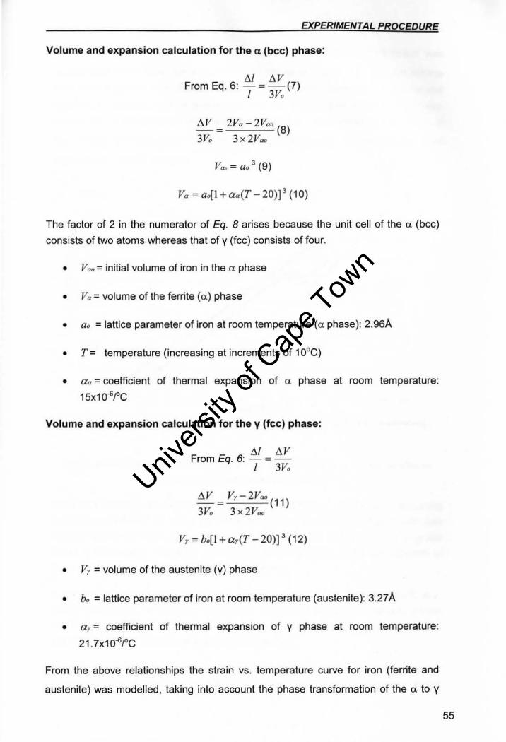
EXPERIMENTAL PROCEDURE
Volume and expansion calculation for the a (bee) phase:
III Il V From Eq . 6: - ~ - (7)
I 3V,
IlV ~ 2V. - 2V., (8) 3V.. 3x2Vao
V. ~ aoll + aa(T - 20)]' (10)
The factor of 2 in the numerator of Eq. 8 arises because the unit cell of the Cl (bee)
consists of two atoms whereas that of V (fcc) consists of fOUf.
• V /III> = initial volume of iron in the a. phase
• Va = volume of the ferrite (0) phase
• a .. = lattice parameter of iron at room temperature (0 phase): 2.96A
• T = temperature (increasing at increments of 10°C)
• ao: = coefficient of thermal expansion of a phase at room temperature:
15x10~rC
Volume and expansion calculation for the V (fcc) phase:
III IlV From Eq. 6: - ~ -
I 3V,
IlV V,- 2Voo ( ) -~ 11 3V.. 3x2Vao
V, ~ bo[ l + a, (T - 20)] ' (12)
• Vr = volume of the austenite (V) phase
• b .. = lattice parameter of iron at room temperature (austenite): 3.27A
• a, = coefficient of thermal expansion of V phase at room temperature:
21 . 7x10~rC
From the above relationships the strain vs. temperature curve for iron (ferrite and
austenite) was modelled, taking into account the phase transformation of the a. to V
55
Univers
ity of
Cap
e Tow
n
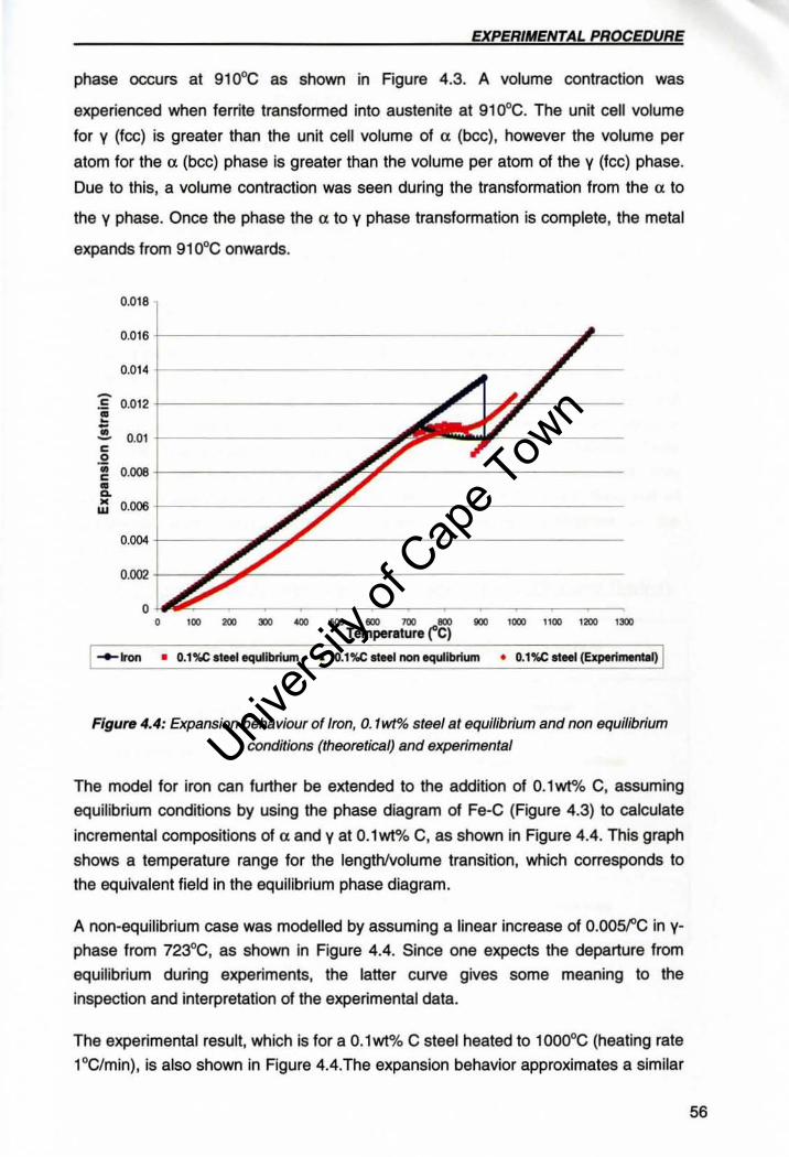
EXPERIMENTAL PROCEDURE
phase occurs at 910°C as shown in Rgure 4.3. A volume contraction was
experienced when ferrite transformed into austenite at 910°C. The unit cell volume
for V (fcc) is greater than the unit cell volume of a (bee), however the volume per
atom for the a (bcc) phase is greater than the volume per atom of the V (fcc) phase.
Due to this, a volume contraction was seen during the transformation from the a to
the V phase. Once the phase the a to y phase transformation is complete, the metal
expands from 910°C onwards.
0.0 18
0.016
0.014
~ 0.01 2 • -E 0.01 e 0 .. 0.006 e • 0. • 0.006 w
0.004
0 ·002 t-7~~-------------
o o ". ,., '" '" SOD eoo 700 eoo
Temperature rC) IlOO 1000 1100 1200 1300
I ~Iron • O.1%C ateel equlibrit.m .. D.l%(: steel non equlibrium • O.1%C steel (Experimanud) I
Figure 4.4: Expansion behaviour of Iron, O. 1wt% stBel at equilibrium and non equilibrium
conditions (theoretical) and experimental
The model for iron can further be extended to the addition of 0.1 wt% C, assuming
equilibrium conditions by using the phase diagram of Fe-C (Figure 4.3) to calculate
incremental compositions of ex and y at 0.1wt% C, as shown in Figure 4.4. This graph
shows a temperature range for the lengthlvolume transition, which corresponds to
the equivalent field in the equilibrium phase diagram.
A non-equilibrium case was modelled by assuming a linear increase of O.OOSf C in y
phase from 723°C, as shown in Figure 4.4. Since one expects the departure from
equilibrium during experiments, the latter curve gives some meaning to the
inspection and interpretation of the experimental data.
The experimental result, which is for a 0.1wt% C steel heated to 1000°C (heating rate
1°C/min), is also shown in Figure 4.4.The expansion behavior approximates a similar
56
Univers
ity of
Cap
e Tow
n
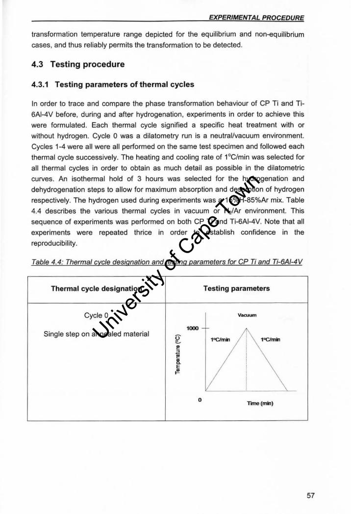
EXPERIMENTAL PROCEDURE
transformation temperature range depicted for the equilibrium and non-equilibrium
cases, and thus reliably permits the transformation to be detected.
4.3 Testing procedure
4.3.1 Testing parameters of thermal cycles
In order to trace and compare the phase transformation behaviour of CP Ti and Ti·
6AI-4V before, during and after hydrogenation. experiments in order to achieve this
were formulated. Each thermal cycle signified a specific heat treatment with or
without hydrogen. Cycle 0 was a dilatometry run is a neutral/vacuum environment.
Cycles 1-4 were all were all performed on the same test specimen and followed each
thermal cycle successively. The heating and cooling rate of 1°C/min was selected for
all thermal cycles in order to obtain as much detail as possible in the dilatometric
curves. An isothermal hold of 3 hours was selected for the hydrogenation and
dehydrogenation steps to allow for maximum absorption and desorption of hydrogen
respectively. The hydrogen used during experiments was a 15%H-85%Ar mix. Table
4.4 describes the various thermal cycles in vacuum or H2/Ar environment This
sequence of experiments was performed on both CP Ti and Ti-6AI-4V. Note that all
experiments were repeated thrice in order to establish confidence in the
reproducibility.
Table 4.4: Thermal cycle designation and testing parameters for CP Ti and Ti-6AI-4V
Thermal cycle designation Testing parameters
Cycle 0 Vacuum
1000 Single step on annealed material
2: 1OC1m1n 1OC1 .....
• " • !I. E !!
0 Tme(min)
57
Univers
ity of
Cap
e Tow
n
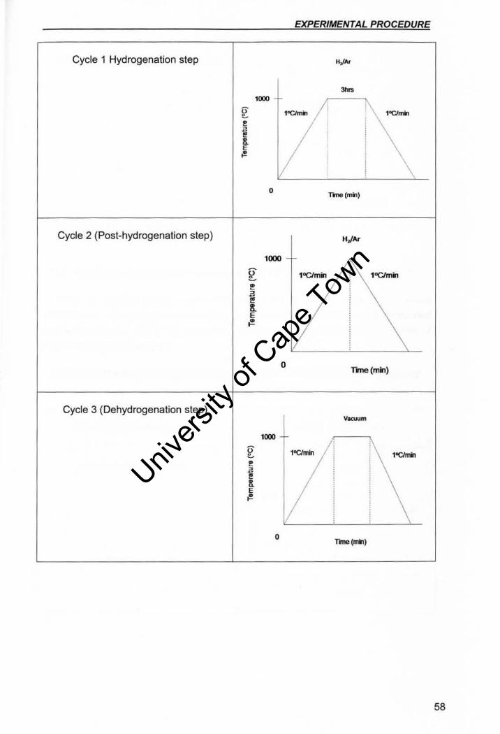
Cycle 1 Hydrogenation step
Cycle 2 (Post-hydrogenation step)
Cycle 3 (Dehydrogenation step)
2: • i E ~
"XX>
o
1000
o
1000
o
EXPERIMENTAL PROCEDURE
Ttne(nm)
1"C1min 1"C1min
rme(mil)
58
Univers
ity of
Cap
e Tow
n
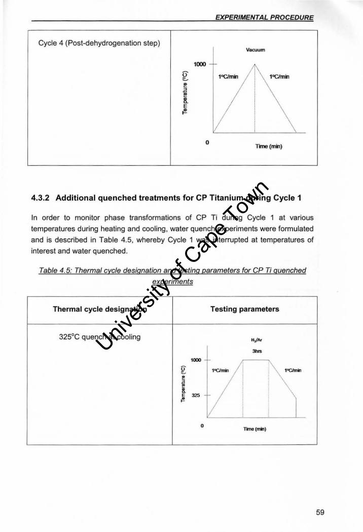
EXPERIMENTAL PROCEDURE
Cycle 4 (Post-dehydrogenation step) Vacuum
1000
o rme(mi1)
4.3.2 Additional quenched treatments for CP Titanium during Cycle 1
In order to monitor phase transformations of CP Ti during Cycle 1 at various
temperatures during heating and cooling, water quench experiments were formulated
and is described in Table 4.5, whereby Cycle 1 was interrupted at temperatures of
interest and water quenched.
Table 4.5: Thermal cycle designation and testing parameters for CP Ti quenched
experiments
Thermal cycle designation Testing parameters
325°C quench at cooling H/"
"'" 1000
E l OCI"*' l'C1"*'
• I , ~
325
.
0 Tme(nWl}
59
Univers
ity of
Cap
e Tow
n
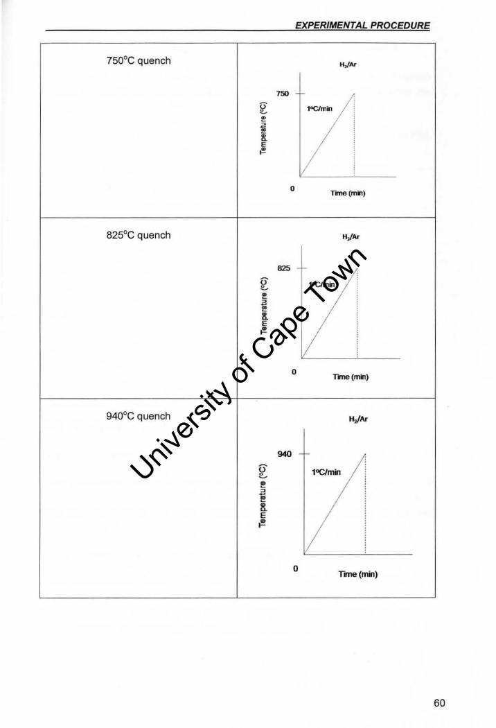
EXPERIMENTA L PROCEDURE
750°C quench HJ'"
750
~ 1OC1mil
• t E ~
0 TIne(nm)
825°C quench HJ'"
825 , 2: 1"C1mh
• i! • 8. E ~
0 Tme(mil)
940°C quench ttJAr
940
[) 1"C1m'" "-• j e x. E I!
0 Tme (min)
60
Univers
ity of
Cap
e Tow
n
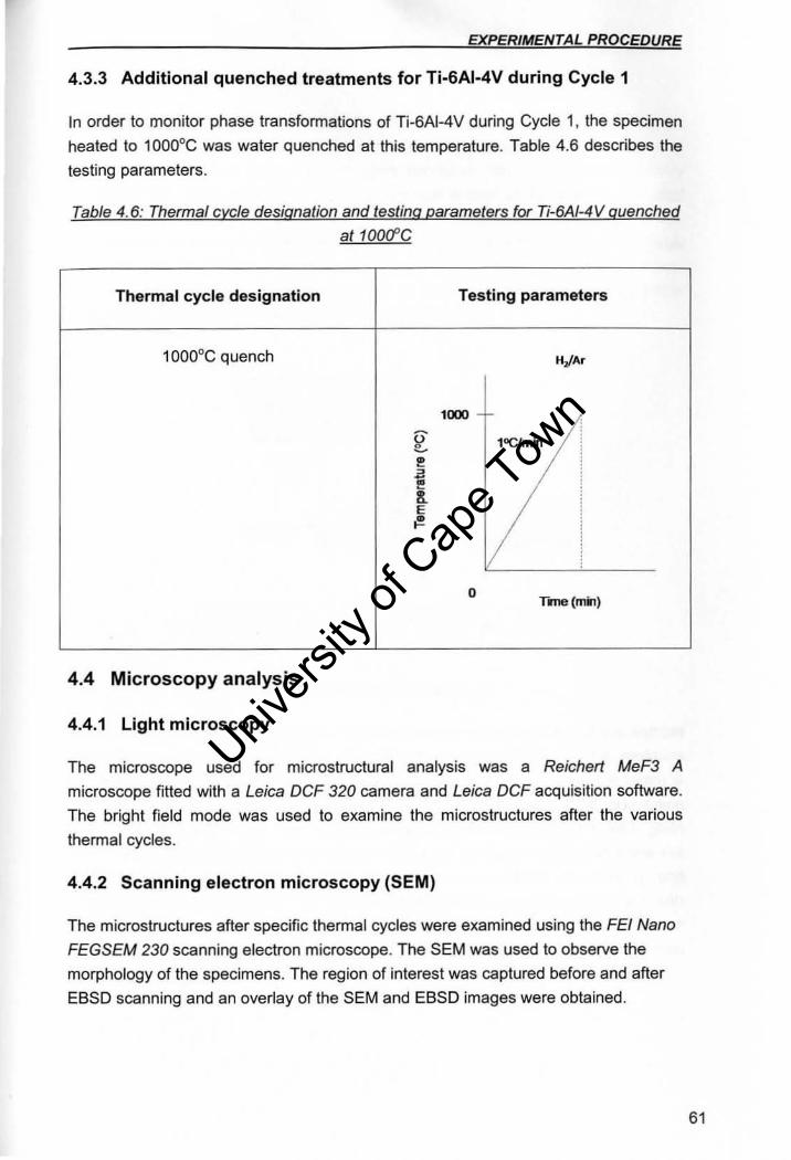
EXPERIMENTAL PROCEDURE
4.3.3 Additional quenched treatments for Ti-6AI-4V during Cycle 1
In order to monitor phase transformations of Ti~6AI~4V during Cycle 1, the specimen
heated to 1Oaaoe was water quenched at this temperature. Table 4.6 describes the
testing parameters.
Table 4.6: Thermal cycle designation and testing parameters for Ti-6AI-4 V quenched
at 100(fC
Thermal cyc le designation Testing parameters
1 aaaoc quench H,jA<
1000
0- 1"C/ma, "-~
~ 1 8. E I! !
, , 0
Tme(mr.)
4.4 Microscopy analysis
4.4.1 Light microscopy
The microscope used for microstructural analysis was a Reichert MeF3 A
microscope fitted with a Leica DCF 320 camera and Leica DCF acquisition software.
The bright field mode was used to examine the microstructures after the various
thennal cycles.
4.4.2 Scanning electron microscopy (SEM)
The microstructures after specific thermal cycles were examined using the FEI Nano
FEGSEM 230 scanning electron microscope. The SEM was used to observe the
morphology of the specimens. The region of interest was captured before and after
EBSD scanning and an overlay of the SEM and EBSD images were obtained.
61
Univers
ity of
Cap
e Tow
n
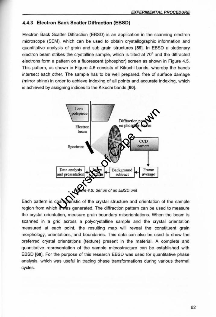
EXPERIMENTAL PROCEDURE
4.4.3 Electron Back Scatter Diffraction (EBSD)
Electron Back Scatter Diffraction (EBSD) is an application in the scanning electron
microscope (SEM). which can be used to obtain crystallographic information and
quantitative analysis of grain and sub grain structures [59]. In EBSD a stationary
electron beam strikes the crystalline sample, which is tilted at 70° and the diffracted
electrons form a pattem on a fluorescent (phosphor) screen as shown in Figure 4.5.
This pattern, as shown in Figure 4.6 consists of Kikuchi bands, whereby the bands
intersect each other. The sample has to be well prepared , free of surface damage
(mirror shine) in order to achieve indexing of all points and accurate indexing, which
is achieved by assigning indices to the Kikuchi bands [60).
ElectrDn
"".un
Specimen
Data analysis Index and ~S<:ntation panem
Difiraeljon plmem phosphDr screen
Background subtract
cco ...,.,.
Frame average
F;gure 4.5: Set up of an EBSD unit
Each pattern is characteristic of the crystal structure and orientation of the sample
region from which it was generated. The diffraction pattern can be used to measure
the crystal orientation, measure grain boundary misorientations. When the beam is
scanned in a grid across a polycrystalline sample and the crystal orientation
measured at each point, the resulting map will reveal the constituent grain
morphology, orientations, and boundaries. This data can also be used to show the
preferred crystal orientations (texture) present in the material. A complete and
quantitative representation of the sample microstructure can be established with
EBSD (SO). For the purpose of this research EBSD was used for quantitative phase
analysis, which was useful in tracing phase transformations during various thermal
cycles.
62
Univers
ity of
Cap
e Tow
n
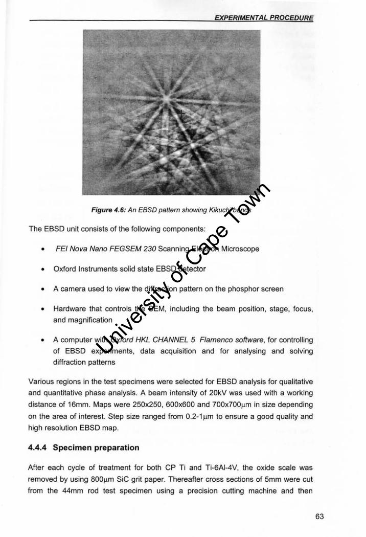
EXPERIMENTAL PROCEDURE
Figure 4.6: An EBSD pattern showing Kikuchi bands
The EBSD unit consists of the following components:
• FEI Nova Nano FEGSEM 230 Scanning Electron Microscope
• Oxford Instruments solid state EBSD detector
• A camera used to view the diffraction pattern on the phosphor screen
• Hardware that controls the SEM, including the beam position, stage, focus,
and magnification
• A computer with Oxford HKL CHANNEL 5 Flamenco software, for controlling
of EBSD experiments. data acquisition and for analysing and solving
diffraction patterns
Various regions in the test specimens were selected for EBSD analysis for qualitative
and quantitative phase analysis. A beam intensity of 20kV was used with a working
distance of 16mm. Maps were 250x250, 600x600 and 700x700~m in size depending
on the area of interest. Step size ranged from O .2- 1 ~m to ensure a good quality and
high resolution EBSD map.
4.4.4 Specimen preparation
After each cycle of treatment for both CP Ti and Ti-6AI-4V, the oxide scale was
removed by using 800Jlm SiC grit paper. Thereafter cross sections of 5mm were cut
from the 44mm rod test specimen using a precision cutting machine and then
63
Univers
ity of
Cap
e Tow
n
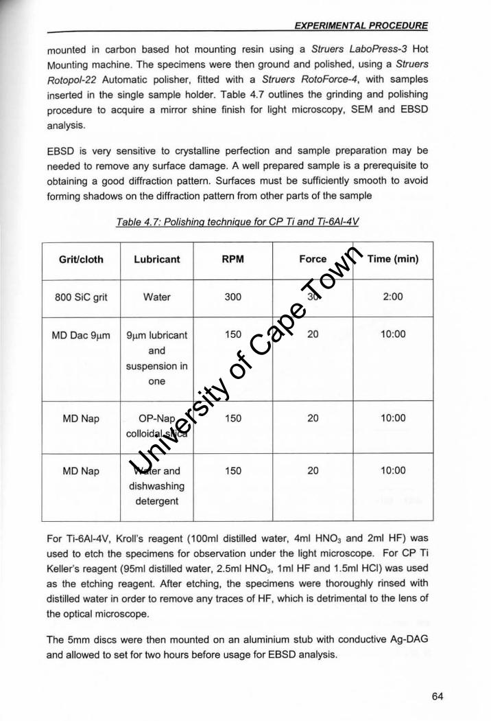
EXPERIMENTAL PROCEDURE
mounted in carbon based hot mounting resin using a Struers LaboPress-3 Hot
Mounting machine. The specimens were then ground and polished, using a Struers
Rotopol-22 Automatic polisher, fitted with a Struers RotoForce-4, with samples
inserted in the single sample holder. Table 4.7 outlines the grinding and polishing
procedure to acquire a mirror shine finish for light microscopy, SEM and EBSD
analysis.
EBSD is very sensitive to crystalline perfection and sample preparation may be
needed to remove any surface damage. A well prepared sample is a prerequisite to
obtaining a good diffraction pattern. Surfaces must be sufficiently smooth to avoid
forming shadows on the diffraction pattern from other parts of the sample
Table 4.7: Polishing technique for CP Ti and Ti-6AI-4V
Grit/cloth Lubricant RPM Force Time (min)
800 SiC grit Water 300 30 2:00
MD Dacg~m 9~m lubricant 150 20 10:00
and
suspension in
one
MD Nap OP-Nap 150 20 10:00
colloidal silica
MD Nap Water and 150 20 10:00
dishwashing
detergent
For Ti-6AI-4V, Kroll's reagent (100ml distilled water, 4ml HNO, and 2ml HF) was
used to etch the specimens for observation under the light microscope. For CP Ti
Keller's reagent (g5ml distilled water, 2.5ml HNO" 1 ml HF and 1.5ml HCI) was used
as the etching reagent. After etching. the specimens were thoroughly rinsed with
distilled water in order to remove any traces of HF. which is detrimental to the lens of
the optical microscope.
The Smm discs were then mounted on an aluminium stub with conductive Ag-DAG
and allowed to set for two hours before usage for EBSD analysis.
64
Univers
ity of
Cap
e Tow
n
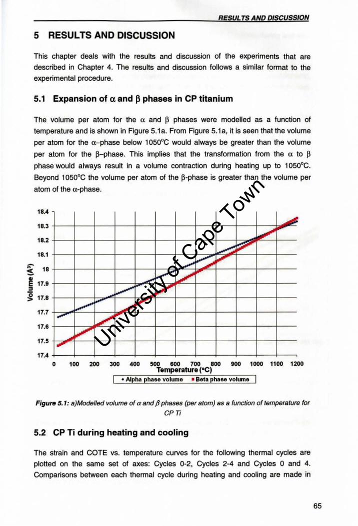
RESUL TS AND DISCUSSION
5 RESULTS AND DISCUSSION
This chapter deals with the results and discussion of the experiments that are
described in Chapter 4. The results and discussion follows a similar format to the
experimental procedure.
5.1 Expansion of a and p phases in CP titanium
The volume per atom for the a and p phases were modelled as a function of
temperature and is shown in Figure S.la. From Figure 5.18, it is seen that the volume
per atom for the a- phase below 10S0oe would always be greater than the volume
per atom for the p-phase. This implies that the transformation from the a to p
phase would always result in a volume contraction during heating up to 10S0oe .
Beyond 10S0oe the volume per atom of the p~phase is greater than the volume per
atom of the a·phase.
18."
18.3
1 •. 2
1 •. 1
.J
~ '"" .....:;
" - ...... ~ " 18 c( - V -..". ~ " g
17.9
17 .•
17.7
17.6
17.S
17."
.... ......... V
V .." " I ..... ./' ~
I ......
0100 m ~ ~ _ ~ ~ ~ _ 1~11001m
Temperature (OC) I • Alpha phase volume • aeta phase volume I
Figure 5.1: a)Modelled volume of a and P phases (per atom) as a function of temperature for
cpr;
5.2 CP Ti during heating and cooling
The strain and COTE vs. temperature cUlVes for the following thermal cycles are
ploned on the same set of axes: Cycles 0-2. Cycles 2-4 and Cycles 0 and 4.
Comparisons between each thermal cycle during heating and cooling are made in
65
Univers
ity of
Cap
e Tow
n
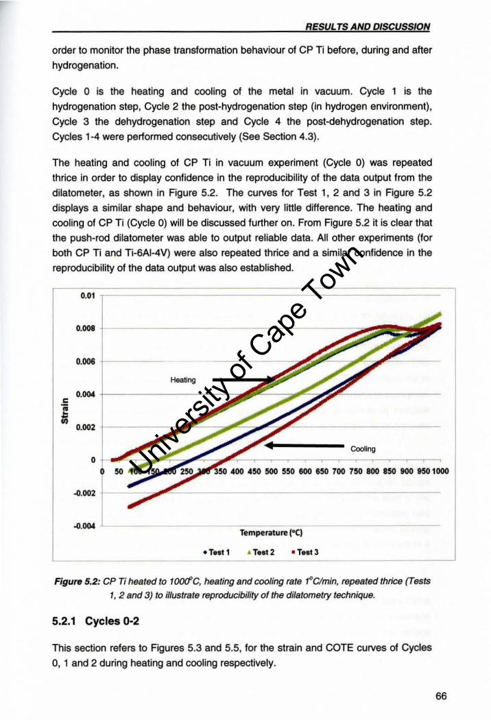
RESULTS AND DISCUSSION
order to monitor the phase transformation behaviour of CP Ti before, during and after
hydrogenation.
Cycle 0 is the heating and cooling of the metal in vacuum. Cycle 1 is the
hydrogenation step. Cycle 2 the post-hydrogenation step (in hydrogen environment),
Cycle 3 the dehydrogenation step and Cycle 4 the post-dehydrogenation step.
Cycles 1 -4 were performed consecutively (See Section 4.3).
The heating and cooling of CP Ti in vacuum experiment (Cycle 0) was repeated
thrice in order to display confidence in the reproducibility of the data output from the
dilatometer, as shown in Figure 5.2. The curves for Test 1, 2 and 3 in Figure 5.2
displays a similar shape and behaviour, with very little difference. The heating and
cooling of CP Ti (Cycle 0) will be discussed further on. From Figure 5.2 it is clear that
the push-rod dilatometer was able to output reliable data. AU other experiments (for
both CP Ti and Ti-6AI-4V) were also repeated thrice and a similar confidence in the
reproducibility of the data output was also established.
0.01
•. 008
• . 008
Heating ..... c ;; ~
0.002
• 400 4SO 500 550 100 ISO 700 7SO 800 850 900 150 1000
-0.002
...... Temperature I-C)
• T •• t 1 . T •• t2 - T •• t3
Figure 5.2: CP Ti heated to 100c/'C, heating and cooling rate 1°C/min, repeated thrice (Tests
1, 2 and 3) to illustrate reproducibility of the dilatometry technique.
5.2.1 Cycles 0-2
This section refers to Figures 5.3 and 5.5, for the strain and COTE curves of Cycles
0, 1 and 2 during heating and cooling respectively.
66
Univers
ity of
Cap
e Tow
n
RESUL TS AND DISCUSSION
The phase transformation behaviour for CP Ti is reported for the three conditions in
this section, i.e. Cycle 0, 1 and 2. Cycle 0 aims to serve as a benchmark for Cycles
1-4, in order to monitor the influence of hydrogen on CP Ti.
The specimen in Cycle 0 expands from room temperature to 600°C at a constant rate
of expansion due to the normal thermal effects during heating, which can be seen by
the strain and COTE curves (See Figure 5.3). From 600-800°C, the specimen
continues to expand, but at a slightly decreased rate of expansion as shown by the
strain and COTE curves. This is not likely to coincide with a phase transformation,
since early transformation from 600°C was unexpected. This is because an unalloyed
metal i.e. CP Ti should display a single temperature below which everything should
be a-phase and above this temperature everything should be l3-phase viz. l3-transus
(883°C).
The a to 13 phase transformation is expected to accompany a volume contraction,
since the volume per atom of the a phase is larger than the volume per atom of the 13 phase as shown in Figure 5.1. The specimen experienced a significant change in
COTE values from the 800-940°C. This associated volume contraction is indicative of
the a to 13 phase transformation. From 940°C the specimen expands normally as
shown by the strain and COTE curves up to 1000°C, signifying the existence of the
single phase 13. Since the l3-transus is described as the lowest temperature that
maximum l3-phase will exist, the l3-transus can be taken as 940°C in this study. This
l3-transus is slightly higher than the reported l3-transus (883°C). The discrepancy in
the reported and experimental l3-transus may be due to the fact that the specimen
was continuously heated (1°C/min). In addition to this, the presence of residual
elements i.e. Fe, would result in the transformation of the a to 13 phase to occur over
a temperature range, rather than at a single temperature.
After the heating step, the specimen in Cycle 0 was cooled from 1000°C to room
temperature. At 1000°C the single l3-phase exists. During cooling, there is an abrupt
change in the contraction rate at approximately 860°C, which signifies the start of the
reverse transformation of the 13 to a-phase (See Figure 5.5). The contraction rate
stabilizes below 780°C, which indicates the end of the reverse transformation. During
cooling from 780°C to room temperature the specimen then continues to contract at a
more or less constant rate due to the normal effects upon cooling.
Cycle 1 is the hydrogenation thermal cycle. This thermal cycle should consist of the
a-phase at the start of Cycle 1. The specimen in Cycle 1 deviates slightly from Cycle
o at 400°C. The solubility of hydrogen in the a-phase is relatively low in comparison
to the solubility in the l3-phase. However, hydrogen can increase the lattice
parameter of the a-phase from 400°C onwards. From 400-550°C the rate of
67
Univers
ity of
Cap
e Tow
n
RESUL TS AND DISCUSSION
expansion shows a slight increase as shown in Figure 5.3, which can thus be
attributed to the increase in the lattice parameter of the a-phase [61].
The progression of the phase transformations in CP Ti with the addition of hydrogen,
can be traced using the Ti-H phase diagram (See Figure 5.4), coupled with the use of
dilatometry. The specimen in Cycle 1 deviates significantly from Cycle 0 at 550°C. At
temperatures below 550°C, the uptake of hydrogen is relatively low, and above
550°C the uptake of hydrogen occurs more rapidly [41]. Hence, point A in Figure 5.4
signifies the start of hydrogen uptake. From 550-750°C, the specimen continues to
expand, but the rate of expansion increases and then decreases after 750°C. This
rise in the COTE values (See Figure 5.3) can be attributed to the increase in
hydrogen uptake, whereby the solid solution of hydrogen occurs in the a-phase. The
path along point A to B, in Figure 5.4 shows this increase in the hydrogen dissolution
up to 750°C. From approximately 750°C, the specimen continues to expand but at a
decreasing rate of expansion, which signals the a to p phase transformation. The
rate of expansion increases thereafter. The path from point B to C in Figure 5.4
marks this transformation. It is difficult to identify the p-transus, since hydrogen will
continue to dissolve and expand the p-phase. However, the p-transus should
definitely be below the value for the vacuum cycle (Cycle 0) and is possibly in the
vicinity of 875°C.
Above 875°C, the specimen is in the p-phase field. The specimen continues to
expand but at an increasing rate and then the rate decreases above 940°C. The
increase in the COTE values can be attributed to the absorption of hydrogen in the p
phase, which results in an increase in the lattice parameter of the p-phase. When
heating from 940-1000°C, the decrease in expansion rate (as shown in the strain and
COTE curves for Cycle 1) may be due to two reasons. One of the reasons may be
that from point 0 (940°C) in the Figure 5.4, an increase in temperature results in the
specimen moving along the (PTi)/(PTi)+G boundary, which would result in the loss of
hydrogen gas from the specimen. The second reason may be that the increase in the
rate of expansion (COTE values) caused by hydrogen absorption slows down as the
rate of hydrogen absorption reaches saturation. Thus, there is an apparent decrease
in the COTE values as the temperature rises.
Assuming that equilibrium was not achieved, the points plotted to form the curve
extending from A to E in Figure 5.4, represents the maximum transformation
temperatures. Hence, it is reasonable to indicate a shaded region (±50-75°C) below
this curve (See Figure 5.3), which indicates the broader possible hydrogen uptake
behaviour as a function of temperature and heating rate.
In Cycle 0 the a to p phase transformation occurred from 800-940°C, but the addition
of hydrogen is known to lower the a to p transformation temperature. This lowering of
68
Univers
ity of
Cap
e Tow
n
RESUL TS AND DISCUSSION
the transformation temperature can be seen from 750-875°C in Cycle 1, whereby the
rate of expansion changes as shown by the strain and COTE curves signifying this
phase transformation.
The proposed sequence of phase transformations for Cycle 1 during heating can be
summarized as follows:
Where UH and I3H represent hydrogen in solid solution in the U and 13 phases
respectively and G is hydrogen gas.
After the end of the heating step in Cycle 1, the specimen at 1000°C is in the l3-phase
field. During cooling from 1000°C to 750°C, the specimen in Cycle 1 experiences a
continuous change in the COTE values, with the rate of contraction decreasing then
increasing (See Figure 5.5). This change in the COTE values can be attributed to the
increase in the uptake of hydrogen in the l3-phase, and follows a path from point A to
B as shown in Figure 5.6.
During cooling from 750°C to 300°C, the specimen in Cycle 1 exhibits a very gradual
decrease in the contraction rate as shown by the strain and COTE curves. This
suggests that no additional hydrogen uptake (or at least very little) occurred in this
temperature interval. The progression from point B to C thus occurs, as shown in
Figure 5.6, which indicates a relatively small change in hydrogen uptake during
cooling over the relevant interval.
At 300°C, the specimen in Cycle 1 once again deviates from Cycle o. During cooling
from 300°C to 220°C a continuous change in the contraction rate is observed and a
volume expansion is seen when cooling from 275°C to 250°C. These changes can be
attributed to the eutectoid transformation of the I3H to uH+hydride phase
transformation, as shown by the path from point C to 0 in Figure 5.6. This eutectoid
transformation occurs in the shaded region (40-44at%H), as shown in Figure 5.6.
Hydrogen is able to lower the l3-transus of CP Ti to -300°C as seen by the Ti-H
phase diagram. From 220°C to room temperature the COTE values remained more
or less constant, signifying that the 13 to u+hydride phase transformation was
complete. The final phases present after the completion of Cycle 1 (heating and
cooling) was a mixture of the u+hydride phases.
The proposed sequence of phase transformations for Cycle 1 during cooling can be
summarised as follows:
PH ~ aJl + hydride
69
Univers
ity of
Cap
e Tow
n
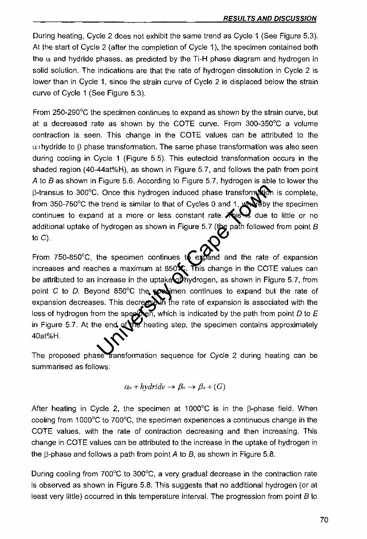
RESUL TS AND DISCUSSION
During heating, Cycle 2 does not exhibit the same trend as Cycle 1 (See Figure 5.3).
At the start of Cycle 2 (after the completion of Cycle 1), the specimen contained both
the a and hydride phases, as predicted by the Ti-H phase diagram and hydrogen in
solid solution. The indications are that the rate of hydrogen dissolution in Cycle 2 is
lower than in Cycle 1, since the strain curve of Cycle 2 is displaced below the strain
curve of Cycle 1 (See Figure 5.3).
From 250-290°C the specimen continues to expand as shown by the strain curve, but
at a decreased rate as shown by the COTE curve. From 300-350°C a volume
contraction is seen. This change in the COTE values can be attributed to the
a+hydride to [3 phase transformation. The same phase transformation was also seen
during cooling in Cycle 1 (Figure 5.5). This eutectoid transformation occurs in the
shaded region (40-44at%H), as shown in Figure 5.7, and follows the path from point
A to 8 as shown in Figure 5.6. According to Figure 5.7, hydrogen is able to lower the
[3-transus to 300°C. Once this hydrogen induced phase transformation is complete,
from 350-750°C the trend is similar to that of Cycles 0 and 1, whereby the specimen
continues to expand at a more or less constant rate. This is due to little or no
additional uptake of hydrogen as shown in Figure 5.7 (the path followed from point 8
to C).
From 750-850°C, the specimen continues to expand and the rate of expansion
increases and reaches a maximum at 850°C. This change in the COTE values can
be attributed to an increase in the uptake of hydrogen, as shown in Figure 5.7, from
point C to D. Beyond 850°C the specimen continues to expand but the rate of
expansion decreases. This decrease in the rate of expansion is associated with the
loss of hydrogen from the specimen, which is indicated by the path from point 0 to E
in Figure 5.7. At the end of the heating step, the specimen contains approximately
40at%H.
The proposed phase transformation sequence for Cycle 2 during heating can be
summarised as follows:
all + hydride ~ flu ~ flu + (G)
After heating in Cycle 2, the specimen at 1000°C is in the [3-phase field. When
cooling from 1 OOO°C to 700°C, the specimen experiences a continuous change in the
COTE values, with the rate of contraction decreasing and then increasing. This
change in COTE values can be attributed to the increase in the uptake of hydrogen in
the [3-phase and follows a path from point A to 8, as shown in Figure 5.8.
During cooling from 700°C to 300°C, a very gradual decrease in the contraction rate
is observed as shown in Figure 5.8. This suggests that no additional hydrogen (or at
least very little) occurred in this temperature interval. The progression from point 8 to
70
Univers
ity of
Cap
e Tow
n
RESULTS AND DISCUSSION
C thus occurs as shown in Figure 5.8, which indicates a small change in hydrogen
uptake during cooling over the relevant interval.
During cooling from 30QoC to 220°C in Cycle 2, a continuous change in the
contraction rate is observed and a volume contraction is seen cooling from 275°C to
250°C. These changes can be attributed due to the 13 to a+hydride phase
transformation, as shown in Figure 5.8 (path followed from point C to D). Hydrogen
thus lowered the l3-transus to this temperature. From 220°C to room temperature the
COTE values remained more or less constant signifying that the 13 to a+hydride
phase transformation was complete. The final phases present after the completion of
Cycle 2 (heating and cooling) was a mixture of the a+hydride phases.
The proposed phase transformation sequence for Cycle 2 during cooling can be
summarised as follows:
p" ---+ lMi + hydride
The strain curve for the Cycle 2 during cooling is displaced below the strain curve of
Cycle 1 during cooling as shown in Figure 5.5. This is as a result of the different initial
lengths 10 of the specimens values for each thermal cycle (See Figure 5.5). For
Cycle 1 the final length " is greater than 10. This suggests that the rate of hydrogen
absorption in Cycle 1 was greater than that of Cycle 2. This was due to the prior existence of hydrogen at the start of Cycle 2.
71
Univers
ity of
Cap
e Tow
n
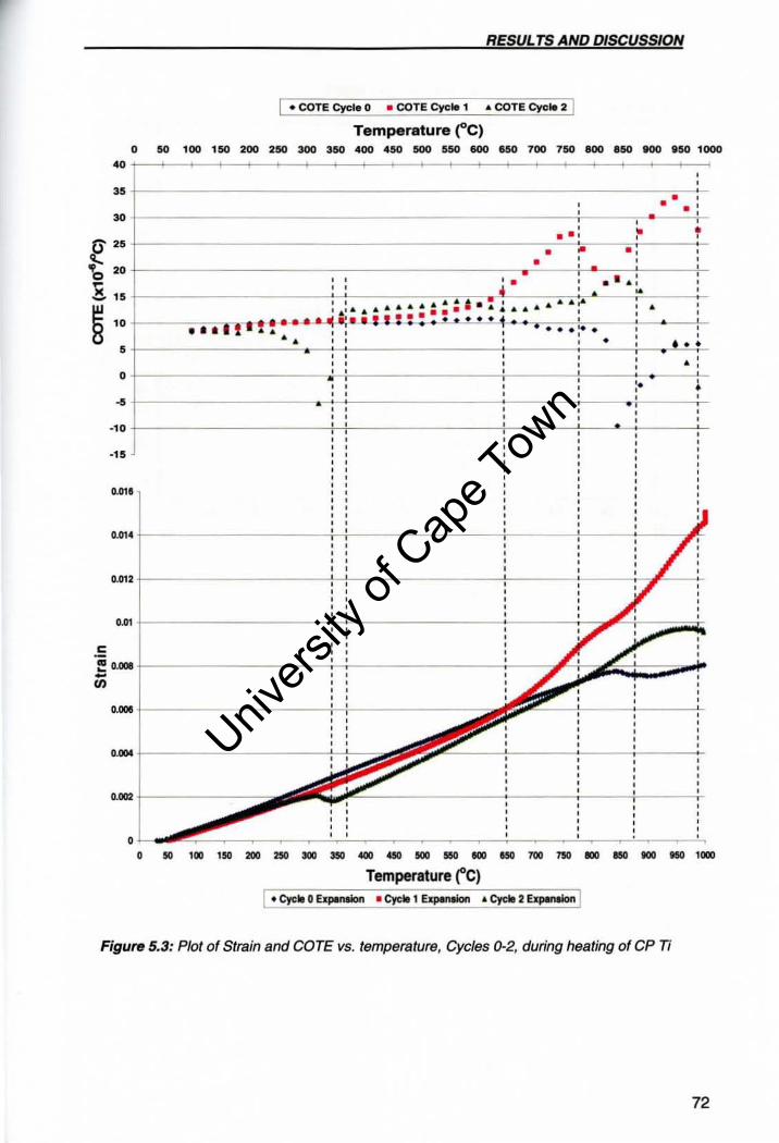
RESULTS AND DISCUSSION
• COTE Cycle 0 • COTE Cycle 1 .. COTE CycIe:Z I Temperature f C)
o 50 100 150 200 250 300 350 400 450 !500 550 IlOO S50 700 7110 800 850 toO .50 1000
'" , ,
" • , 30
, • , , • , • , ,
S! " '0 ,. ';c
" -§ ,.
• • ..
.,.
, • • • . , , , , , , • ~ " ,
• , , , , • , , • ,
•• , , , , j ' , . , , , , , • ,
, , • • • I · , • • ., , , I I ....... .. ...... • • • • • • • •
~ •••. ~ :, •• , 'J:_:_: • , , , • • • • • • • • • , , • ,
• • • ' ! ' ... .to I : • • • .- • , , ..... "
, , , , • , • • • ... -'- ' , , ~-, , , , , , , , , • , , , , , , • , '. , , , , , • , , , , ..... , +, , , , , , , ' -
." , , , , , ,
11.01'
.m. t--------------------4-+-----------------r------~----~.----"'~
om.I----------t--l--------t-------
om t-------------------,
.E ~ o~ t-------------------;-'-----------------r---c~-r~~+;;;~~ Ul
0." j-------------------H -------------:;;;
... t_-----------------~_}~ ,. , , , , .. ~O-----------------~.--------""------t-------~
o. _______ ~ __________ _ Temperature ("e)
.. eye .. 0 ErpIneion • Cyc" 1 ~ .. eye":2 E..IpwWDn I
Figure 5.3: Plot of Strain and COTE vs. temperBture, Cycles 0-2, during heating o( CP Ti
72
Univers
ity of
Cap
e Tow
n
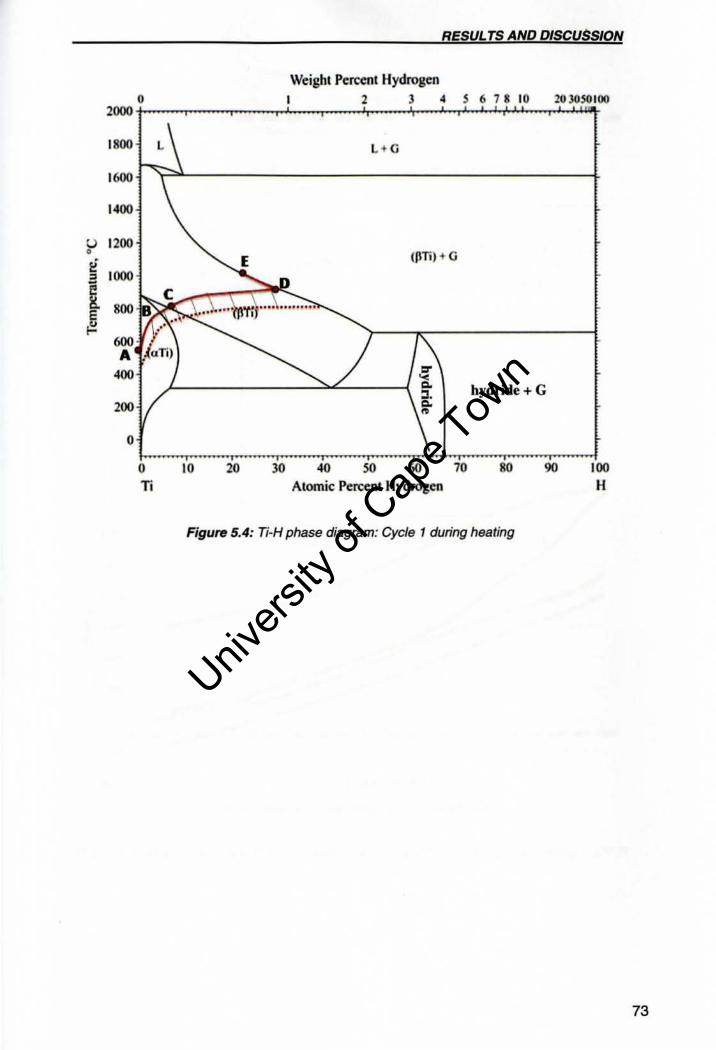
Figure 5.4: Ti-H phase diagram: Cycle 1 during heating
73
Univers
ity of
Cap
e Tow
n
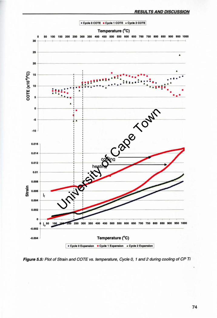
-0
~ 0 ~
.!!. UJ .... 0 0
C ;; .. Ul
RESUL TS AND DISCUSSION
I. eye'-OCaTE • eye. 1 COTE .. eye. 2 COTE I
Temperature r C) ,_.,._----------------" l----------------------------------------------------------•
~ +--------------------------------------------, •
" " ,
.f---------;---'~------c·':,.. , . ....... .. ' -'.. . " ... I .. .. .. • ••
j •• 1 1 l1li '" .. " .t : . ,t' :*s •• ····· . .... .f---------=-T. .. +~._._.,~ .. .. .. . ... ... 'i·~·'-----.. f • .. ... • --4~."7. • ... I .-t-. : I • • ... , ... .. .. ..... II. .. ".. • .. .. , .. .. •
, , • , , , , • , • ,
~ •
. " O.OIlS
0.01.
0.012
0.01
, .... , ...
I, , .... , ...
, • ~- '00 250 300 3SO 400 450 500 550 eoo eo 700 rao toO '50 100 150 1000
... , J
..... Temperature t e)
I .. ere. 0 bpMaIon .. ere .. 1 ExpaneIon ... Cyct. 2 Eap.MIon t
Figure 5.5: Plot of Strain and COTE vs. temperature, Cycle 0, 1 and 2 during cooling of CP Ti
74
Univers
ity of
Cap
e Tow
n
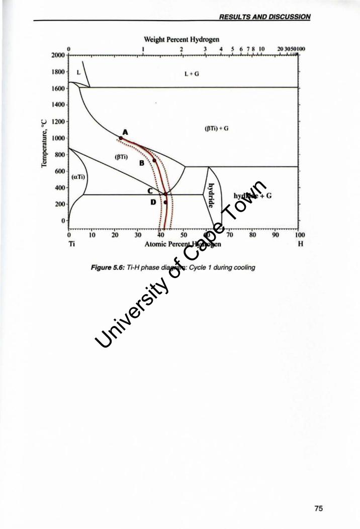
0 2000
1800
1600
1400
U 1200 • Ii
1000 ~ K. 800 C >:!
600 (uTi)
400
200
0
0 Ti
10 20
RESUL TS AND DISCUSSION
Weight Percent Hydrogen I 1 J 4 5 6 78 10 203050100
L- G
A (PTi) + G
....... ~.\ .....
30
" " " ! , . . . D \ , · · · ·
so 60 Atomic Percent Hydrogen
hydride + G
70 80 90 100 H
Figure 5.6: Ti-H phase diagram: Cycle 1 during cooling
75
Univers
ity of
Cap
e Tow
n
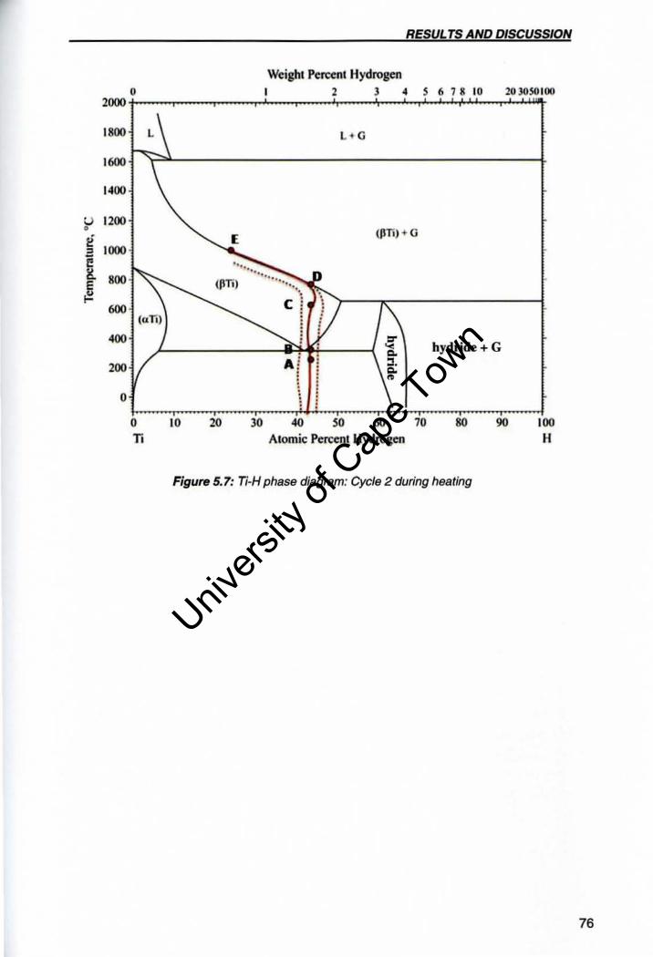
0 2000
1800 L
1600
1400
U 1200 • Ii
1000 " i! It 800 E ~
600 (uTi)
400
200
0
0 n
10 20 30
RESUL TS AND DISCUSSION
Weight Percent Hydrogen 2 3. S 6 78 10 203050100
L d l
(IJTI) + G
A i
i . 40 SO 60 70
Atomic Percent Hydrogen
hydride + G
80 90 100 H
Figure 5.7: Ti-H phase diagram: Cycle 2 during heating
76
Univers
ity of
Cap
e Tow
n
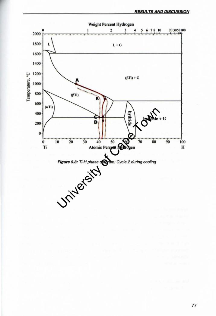
0 2000
1800
1600
1400
U 1200 • Ii
1000 .'! e l!. 800
~ 600
(uTi)
400
200
0
0 Ti
10 20 )0
RESUL TS AND DISCUSSION
Weight Percent Bydrogen 2 J .. 56 7 810 203050 100
L' G
(PTa) + G
Df . .
40 SO 60 70 Alomic Percent Hydrogen
hydride + G
80 90 100 H
Figure 5.8: Ti-H phase diagram: Cycle 2 during cooling
n
Univers
ity of
Cap
e Tow
n
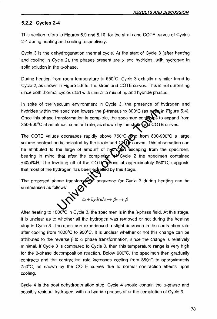
RESUL TS AND DISCUSSION
5.2.2 Cycles 2-4
This section refers to Figures 5.9 and 5.10, for the strain and COTE curves of Cycles
2-4 during heating and cooling respectively.
Cycle 3 is the dehydrogenation thermal cycle. At the start of Cycle 3 (after heating
and cooling in Cycle 2), the phases present are a and hydrides, with hydrogen in
solid solution in the a-phase.
During heating from room temperature to 650°C, Cycle 3 exhibits a similar trend to
Cycle 2, as shown in Figure 5.9 for the strain and COTE curves. This is not surprising
since both thermal cycles start with similar a mix of aH and hydride phases.
In spite of the vacuum environment in Cycle 3, the presence of hydrogen and
hydrides within the specimen lowers the 13-transus to 300°C (as seen in Figure 5.4).
Once this phase transformation is complete, the specimen continues to expand from
350-600°C at an almost constant rate, as shown by the strain and COTE curves.
The COTE values decreases rapidly above 750°C, and from 800-900°C a large
volume contraction is indicated by the strain and COTE curves. This observation can
be attributed to the large of amount of hydrogen escaping from the specimen,
bearing in mind that after the completion of Cycle 2 the specimen contained
±40at%H. The levelling off of the COTE values at approximately 960°C, suggests
that most of the hydrogen has been expelled by this stage.
The proposed phase transformation sequence for Cycle 3 during heating can be
summarised as follows:
After heating to 1000°C in Cycle 3, the specimen is in the 13-phase field. At this stage,
it is unclear as to whether all the hydrogen was removed or not during the heating
step in Cycle 3. The specimen experienced a slight decrease in the contraction rate
after cooling from 1000°C to 900°C. It is unclear whether or not this change can be
attributed to the reverse 13 to a phase transformation, since the change is relatively
minimal. If Cycle 3 is compared to Cycle 0, then this temperature range is very high
for the 13-phase decomposition reaction. Below 900°C, the specimen then gradually
contracts and the contraction rate increases cooling from 880°C to approximately
750°C, as shown by the COTE curves due to normal contraction effects upon
cooling.
Cycle 4 is the post dehydrogenation step. Cycle 4 should contain the a-phase and
possibly residual hydrogen, with no hydride phases after the completion of Cycle 3.
78
Univers
ity of
Cap
e Tow
n
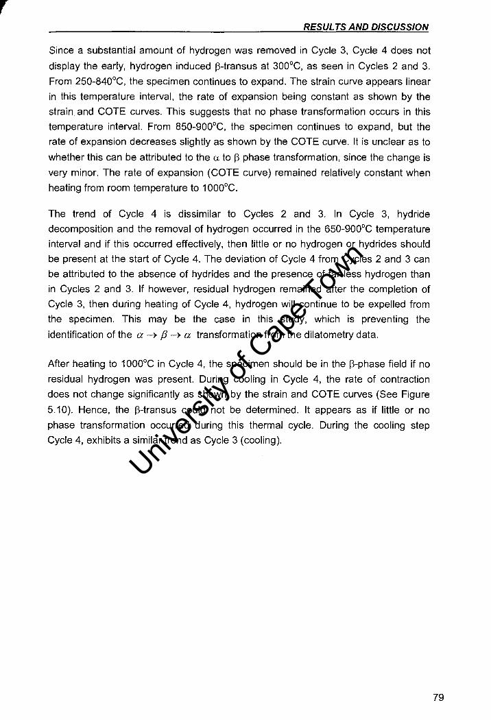
RESUL TS AND DISCUSSION
Since a substantial amount of hydrogen was removed in Cycle 3, Cycle 4 does not
display the early, hydrogen induced 13-transus at 300°C, as seen in Cycles 2 and 3.
From 250-840°C, the specimen continues to expand. The strain curve appears linear
in this temperature interval, the rate of expansion being constant as shown by the
strain and COTE curves. This suggests that no phase transformation occurs in this
temperature interval. From 850-900°C, the specimen continues to expand, but the
rate of expansion decreases slightly as shown by the COTE curve. It is unclear as to
whether this can be attributed to the a to 13 phase transformation, since the change is
very minor. The rate of expansion (COTE curve) remained relatively constant when
heating from room temperature to 1000°C.
The trend of Cycle 4 is dissimilar to Cycles 2 and 3. In Cycle 3, hydride
decomposition and the removal of hydrogen occurred in the 650-900°C temperature
interval and if this occurred effectively, then little or no hydrogen or hydrides should
be present at the start of Cycle 4. The deviation of Cycle 4 from Cycles 2 and 3 can
be attributed to the absence of hydrides and the presence of far less hydrogen than
in Cycles 2 and 3. If however, residual hydrogen remained after the completion of
Cycle 3, then during heating of Cycle 4, hydrogen will continue to be expelled from
the specimen. This may be the case in this study, which is preventing the
identification of the a ~ f3 ~ a transformation from the dilatometry data.
After heating to 1000°C in Cycle 4, the specimen should be in the 13-phase field if no
residual hydrogen was present. During cooling in Cycle 4, the rate of contraction
does not change significantly as shown by the strain and COTE curves (See Figure
5.10). Hence, the 13-transus could not be determined. It appears as if little or no
phase transformation occurred during this thermal cycle. During the cooling step
Cycle 4, exhibits a similar trend as Cycle 3 (cooling).
79
Univers
ity of
Cap
e Tow
n
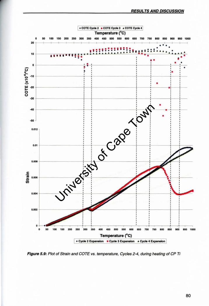
RESULTS AND DISCUSSION
I • COTE eye .. 2 • COTE eye .. 3 .. COTE Cye" 41 Temperature fC) D~_'~~~~ _____________ _
• I • • • • , 1 t • • • I' ,I: . .... +l l .t . I ... : ..... " t-------. .... "T.-'.....--.-. .. • . I .. .. .. .. ... A ... .. ... ... • •• .... , . : : - . • •
• " . " ...... ~ • I •
• • Dt-----------------------,:cl-f---------------------'------ ---------t! --~_c.:-
t '. E ~ .10 +-------------------~~----------------_cc_--~c-------~~:---, - , J;!. • , , , , w .~ t_---------------------_c--"---------------------~------~--------~-:~ b I :
u ' ~ t_------------------~~~------------------~---+-------~-~'--
• ~ t_----------------~-_c----------------~----.~----~.~--+_--
•
0.012
.m j------------t--i------------:---~'-----~-_j;;;;~.
D.""
~
iii D ... ~ - .' I/) • • D .... ~ ",.. -,
D'-'" D ___________________ _
Temperature rC)
Figure 5.9: Plot of Strain and COTE vs. temperature, Cycles 2-4, during heating of CP Ti
80
Univers
ity of
Cap
e Tow
n
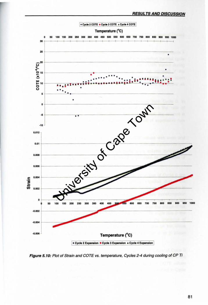
.E I! -'"
.. "
-" ~ 0 , -.!!. w .... ' o "
•
• ,
• •
• 0.012
RESUL TS AND DISCUSs/ON
I. eye .. 2 COTE • eye_ 3 COTE • Cyc ... COTE I Temperature t e)
._-------------------•
• • • • • • • • • • • • • • •••• • ••• I . " • • ••• • • · . 1
• ' +-0 . ..... -a..t " , . . . . ' • • J •• .-.-.... - . - - - . ....... . . - - ' . ' --• • • • • •
••• •
•
•
•• , t-------------------------------------------------------------~
.....
.. ""
.. "" ' .112
• 50 100 150 20D 25(1 300 350 400 U(I 600 ISO 100 750 IlOO 150 IlOO teO 1000
<.112
<.""~~=-----<."" Temperatur. (,C)
I. CyeJe 2 ExpeneJon • eye .. :I EIIP1ntion ... eye .... ExpMalon I
Figure 5.10: Plot of Strain and COTE vs. temperature, Cycles 2-4 during cooling of CP Ti
81
Univers
ity of
Cap
e Tow
n
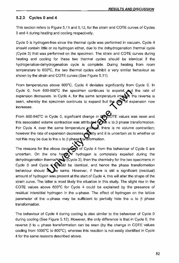
RESUL TS AND DISCUSSION
5.2.3 Cycles 0 and 4
This section refers to Figure 5.11 and 5.12, for the strain and COTE curves of Cycles
o and 4 during heating and cooling respectively.
Cycle 0 is hydrogen-free since the thermal cycle was performed in vacuum. Cycle 4
should contain little or no hydrogen either, due to the dehydrogenation thermal cycle
(Cycle 3) that was performed on the specimen. The strain and COTE curves during
heating and cooling for these two thermal cycles should be identical if the
hydrogenation-dehydrogenation cycle is complete. During heating from room
temperature to 600°C, the two thermal cycles exhibit a very similar behaviour as
shown by the strain and COTE curves (See Figure 5.11).
From temperatures above 600°C, Cycle 4 deviates significantly from Cycle O. In
Cycle 0, from 600-800°C the specimen continues to expand, but the rate of
expansion decreases. In Cycle 4, for the same temperature interval, the reverse is
seen, whereby the specimen continues to expand but the rate of expansion now
increases.
From 800-940°C in Cycle 0, significant change in the COTE values was seen and
this associated volume contraction was attributed to the a to 13 phase transformation.
For Cycle 4, over the same temperature interval, there is no volume contraction;
however the rate of expansion decreases slightly and it is uncertain as to whether or
not this may be due to the a to 13 phase transformation.
The reasons for the above deviations of Cycle 4 from the behaviour of Cycle 0 are
uncertain. On the one hand, if hydrogen is completely expelled during the
dehydrogenation thermal cycle (Cycle 3), then the chemistry for the two specimens in
Cycle 0 and Cycle 4 should be identical, and hence the phase transformation
behaviour should be the same. However, if there is still a significant (residual)
amount of hydrogen was present at the start of Cycle 4, this will alter the shape of the
strain curve. The latter is most likely the situation in this study. The slight rise in the
COTE values above 600°C for Cycle 4 could be explained by the presence of
residual interstitial hydrogen in the a-phase. The effect of hydrogen on the lattice
parameter of the a-phase may be sufficient to partially hide the a to 13 phase
transformation.
The behaviour of Cycle 4 during cooling is also similar to the behaviour of Cycle 0
during cooling (See Figure 5.12). However, the only difference is that in Cycle 0, the
reverse 13 to a phase transformation can be seen (by the change in COTE values
cooling from 1000°C to 800°C), whereas this reaction is not easily identified in Cycle
4 for the same reasons described above.
82
Univers
ity of
Cap
e Tow
n
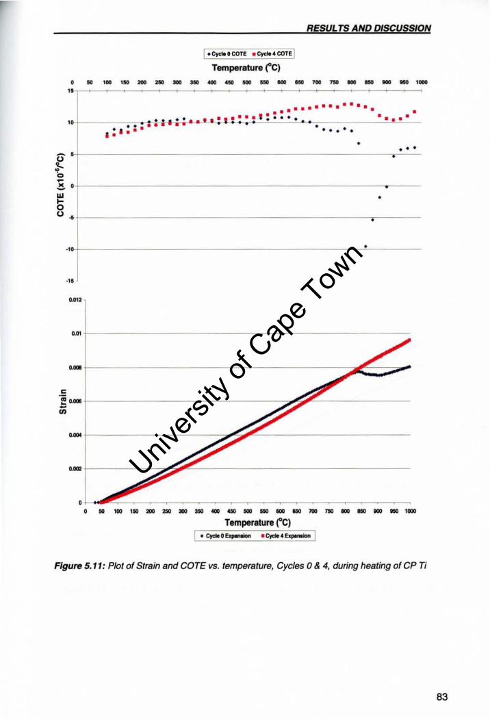
RESULTS AND DISCUSSION
Temperature ("C)
, .. _-----------------",-------------------------------------------------------+---------< • •••••••••••••
I • • • •
L---------:7
' •• .... ' • • • • • " •• • • • -;---------------'. -'-,. _.---", · -1"': I I • • • ----......-.-~.. ~~ . . . : . . . . . . . I ' •
• ••• 0-}-0 -x , -w b
• u •
-" •
-" .,"
.m t---------------------------------------------------------
-~---------------------------~~~
c
~-t-------------------------------~~ -
U> .... =z~=== , 1--000" ::-___________ ~~~~~~
, .. _.---------------Temperature ("C) • CJdt o~ IC)dI4~ I
Figure 5. 11: Plot of Strain and COTE vs. temperature, Cycles 0 & 4, during heating of CP Ti
83
Univers
ity of
Cap
e Tow
n
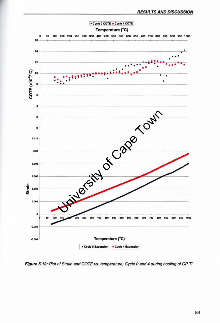
RESUL TS AND DISCUSSION
.. ~"OCOTE . ""COTE Temperature , e ) '.'.'. __ ~m ____________ '_
" .. • .-• •• •
" -o " }-0 ~ • •
...... ..t...!-.!... • .-.-• • • .. . .. • • • • • • • • •• • • -....+. _ • • I' .. · .' .- .. " . '. ~ • • • • • • •• • • • •• • • • -w
b 0 •
• , ,
0.012
.. , .-.-
e °i .... " -'" ....
.. ~" t-_-C_------------------------------
Temperature r C)
Figure 5.12: Plot of Strain and COTE vs. temperature, Cycle 0 and 4 during cooling of CP Ti
84
Univers
ity of
Cap
e Tow
n
RESUL TS AND DISCUSSION
5.3 Ti-6AI-4V during heating and cooling
The strain and COTE vs. temperature curves for the following thermal cycles are
plotted on the same set of axes: Cycles 0-2, Cycles 2-4 and Cycles 0 and 4.
Comparisons between each thermal cycle during heating and cooling are made, in
order to monitor the phase transformation behaviour of Ti-6AI-4V before, during and
after hydrogenation.
Cycle 0 is the heating and cooling of the alloy in vacuum. Cycle 1 is the
hydrogenation step, Cycle 2 is the post-hydrogenation step (in hydrogen
environment), Cycle 3 is the dehydrogenation step and Cycle 4 is the post
dehydrogenation step. Cycles 1-4 were performed consecutively (See Section 4.3.1).
5.3.1 Cycles 0-2
This section refers to Figures 5.13 and 5.14, for the strain and COTE curves of
Cycles 0, 1 and 2 during heating and cooling respectively.
The phase transformation behaviour of the alloy was monitored for Cycles 0, 1 and 2.
The alloy expands due to thermal effects of heating up to 550°C, as shown by the
strain curves (See Figure 5.13). Beyond 550°C, a deviation in the strain and COTE
curves is seen for the three conditions.
Cycle 0 aims to serve as a benchmark for Cycles 1-4, in order to monitor the
influence of hydrogen on the Ti-6AI-4V alloy.
The specimen in Cycle 0 expands from room temperature to 600°C at a constant rate
of expansion due to the normal thermal effects during heating, which can be seen by
the strain and COTE curves (See Figure 5.13). From 600-840°C, the specimen
continues to expand, but at a decreased rate of expansion as shown by the strain
and COTE curves. This is due to the increase in the fraction of the l3-phase for
temperatures above 600°C [19].
The ex to 13 phase transformation is expected to accompany a volume contraction,
since the volume per atom of the ex phase is larger than the volume per atom of the 13
phase as shown in Figure 5.1. The specimen experienced a volume contraction over
the 860-900°C temperature interval, as shown by the strain and COTE curves. This
volume contraction can be attributed to the ex to 13 phase transformation. Above
900°C the specimen expands normally, as shown by the strain and COTE curves up
to 1000°C. The COTE curve continues to change quite rapidly beyond 900°C, which
indicates that the ex to 13 phase transformation is not yet complete. The l3-transus is
probably close to 1000°C, but cannot be accurately determined because the
specimen was not heated above 1000°C
85
Univers
ity of
Cap
e Tow
n
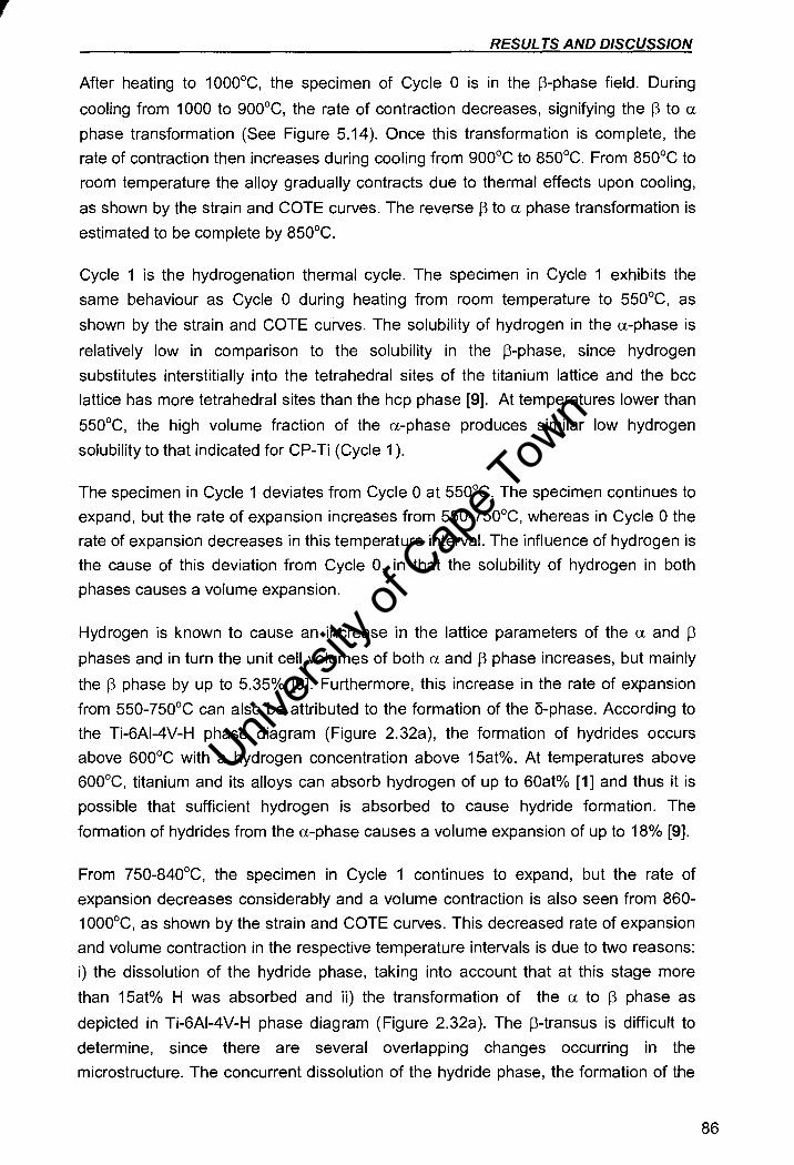
RESUL TS AND DISCUSSION
After heating to 1000°C, the specimen of Cycle 0 is in the f3-phase field. During
cooling from 1000 to 900°C, the rate of contraction decreases, signifying the f3 to a
phase transformation (See Figure 5.14). Once this transformation is complete, the
rate of contraction then increases during cooling from 900°C to 850°C. From 850°C to
room temperature the alloy gradually contracts due to thermal effects upon cooling,
as shown by the strain and COTE curves. The reverse f3 to a phase transformation is
estimated to be complete by 850°C.
Cycle 1 is the hydrogenation thermal cycle. The specimen in Cycle 1 exhibits the
same behaviour as Cycle 0 during heating from room temperature to 550°C, as
shown by the strain and COTE curves. The solubility of hydrogen in the a-phase is
relatively low in comparison to the solubility in the f3-phase, since hydrogen
substitutes interstitially into the tetrahedral sites of the titanium lattice and the bcc
lattice has more tetrahedral sites than the hcp phase [9]. At temperatures lower than
550°C, the high volume fraction of the a-phase produces similar low hydrogen
solubility to that indicated for CP-Ti (Cycle 1).
The specimen in Cycle 1 deviates from Cycle 0 at 550°C. The specimen continues to
expand, but the rate of expansion increases from 550-750°C, whereas in Cycle 0 the
rate of expansion decreases in this temperature interval. The influence of hydrogen is
the cause of this deviation from Cycle 0, in that the solubility of hydrogen in both
phases causes a volume expansion.
Hydrogen is known to cause an increase in the lattice parameters of the a and f3
phases and in turn the unit cell volumes of both a and f3 phase increases, but mainly
the f3 phase by up to 5.35% [9]. Furthermore, this increase in the rate of expansion
from 550-750°C can also be attributed to the formation of the a-phase. According to
the Ti-6AI-4V-H phase diagram (Figure 2.32a), the formation of hydrides occurs
above 600°C with a hydrogen concentration above 15at%. At temperatures above
600°C, titanium and its alloys can absorb hydrogen of up to 60at% [1] and thus it is
possible that sufficient hydrogen is absorbed to cause hydride formation. The
formation of hydrides from the a-phase causes a volume expansion of up to 18% [9].
From 750-840°C, the specimen in Cycle 1 continues to expand, but the rate of
expansion decreases considerably and a volume contraction is also seen from 860-
1000°C, as shown by the strain and COTE curves. This decreased rate of expansion
and volume contraction in the respective temperature intervals is due to two reasons:
i) the dissolution of the hydride phase, taking into account that at this stage more
than 15at% H was absorbed and ii) the transformation of the a to f3 phase as
depicted in Ti-6AI-4V-H phase diagram (Figure 2.32a). The f3-transus is difficult to
determine, since there are several overlapping changes occurring in the
microstructure. The concurrent dissolution of the hydride phase, the formation of the
86
Univers
ity of
Cap
e Tow
n
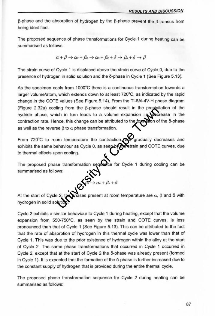
RESUL TS AND DISCUSSION
p-phase and the absorption of hydrogen by the i3-phase prevent the f3-transus from
being identified.
The proposed sequence of phase transformations for Cycle 1 during heating can be
summarised as follows:
a + /3 ~ all +/311 ~ an + plI+ § ~ /311+ 0 --+ f3
The strain curve of Cycle 1 is displaced above the strain curve of Cycle 0, due to the
presence of hydrogen in solid solution and the l)-phase in Cycle 1 (See Figure 5.13).
As the specimen cools from 100QoC there is a continuous transformation towards a
larger volume/atom, which extends down to at least 720°C, as indicated by the rapid
change in the COTE values (See Figure 5.14). From the Ti-6AI-4V-H phase diagram
(Figure 2.32a) cooling from the p-phase should result in the precipitation of the
hydride phase, which in turn leads to a volume expansion i.e. decrease in the
contraction rate. Hence, this change can be attributed to the formation of the 6-phase
as well as the reverse f3 to a phase transformation.
From 720°C to room temperature the contraction rate gradually decreases and
exhibits the same behaviour as Cycle 0, as seen by the strain and COTE curves, due
to thermal effects upon cooling.
The proposed phase transformation sequence for Cycle 1 during cooling can be
summarised as follows:
At the start of Cycle 2. the phases present at room temperature are a., f3 and 6 with
hydrogen in solid solution.
Cycle 2 exhibits a similar behaviour to Cycle 1 during heating. except that the volume
expansion from 550-750oC, as seen by the strain and COTE curves, is less
pronounced than that of Cycle 1 (See Figure 5.13). This can be attributed to the fact
that the rate of absorption of hydrogen in this thermal cycle was lower than that of
Cycle 1. This was due to the prior existence of hydrogen within the alloy at the start
of Cycle 2. The same phase transformations that occurred in Cycle 1 occurred in
Cycle 2, except that at the start of Cycle 2 the 6-phase was already present (formed
in Cycle 1). It is expected that the formation of the i5-phase is further increased due to
the constant supply of hydrogen that is provided during the entire thermal cycle.
The proposed phase transformation sequence for Cycle 2 during heating can be
summarised as follows:
87
Univers
ity of
Cap
e Tow
n
RESULTS AND DISCUSSION
Cycle 2 displays almost identical behaviour to Cycle 1 during cooling as shown by
the strain and COTE curves (See Figure 5.14). The strain curves of Cycle 2 during
cooling is however, displaced below the strain curve of Cycle 1 during cooling . This
suggests that the rate of hydrogen absorption during cooling was greater in Cycle 1
than in Cycle 2. The sequence of phase transformations in Cycle 2 during cooling is
the same as Cycle 2 during cooling and can be summarised as follows:
P" ~GJI +PII +O
ss
Univers
ity of
Cap
e Tow
n
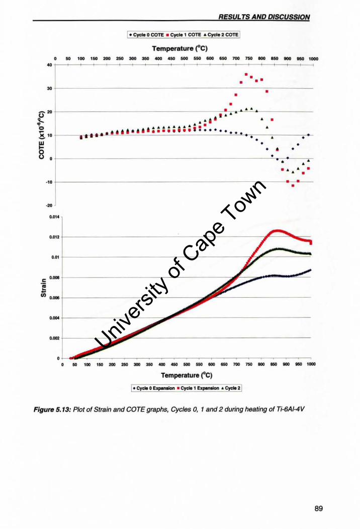
RESULTS AND DISCUSs/ON
• 0 con: • Cyde 1 COTE .. CyeI-. 2 COTE
Temperature r C) ,. __________________ _ ..
• • • • •
~ t_--------------------------------------------~.~--------•
• ~ +--------------------------------~~~ •. ----------u • .to" --
•"-- ... . II ... • • o ... ............ .......... , .. . ~ L___ • ••• • •• •••••• • •• •••••••• ~ 10 1 ._.~.,Jl'""c.~~--~CCCCOC------------cc~c.~-• ._--_c._------.. --
• ~ . 8 ,~ ________________________ ~.~---.
•
." t------------------------------------------------------~~--
... 0..0,.
0.012
."
e ... • ~ -VI ...
I .... t---------------------: ... ~~---------------------------
... 1------------:
,. __________________ _ Temperature t e)
! ... CydI 0 ~ • CydIl &p.n.Ion .. eye .. 21
Figure 5.13: Plot of Strain and COTE graphs, Cycles 0, 1 and 2 during heating of Ti-6AI-4 V
89
Univers
ity of
Cap
e Tow
n
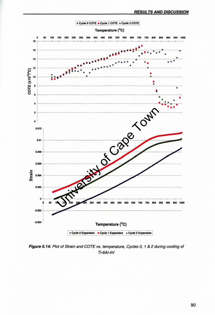
RESULTS AND DISCUSSION
I_ Cycle 0 COTE • ~ 1 COTE .. Cycle 2 COTI! I Temperature re)
.. _------------ ------" I ·
,, +------------------- c-.- -......... .. i • I .. • • • • .-.16 ' .. • •• • ,· ~------------~co·;I .. ·-------•• --------_.,·--. . . . . . . . ... . . . ... t-------~r' •• -'c.,,·c·~· ___ ~· ___ _""_ ______ ___ -.. 12 • • •• - - • e ,! : ..... • • • • o 10 . - . - ..... -=-----~.,---------------.~-------
• - .. ~ : w . t-------------------------------------------------------------------~------------~
8 • .. • t-------------------------------------------~.~----_c_ • • • +-----------------------------",n .... ~ . -.---•••
' t------------------------------------------------------
• 0.012
... +-----------------------------------------------c~~~~------------_c.,~
... t---------------------~~~~------~~~-------c ~ • .. t-----------------c .. ~c-~~----------~~-----------------~
... +-_____ ~ __ ~C-~~C---------_.~~--------------------------------
~ .. +----_c~~0------------------------------------------------------------------
Temperature ("C)
I .. eye .. 0 Expo"*'" • Cycle 1 ExpeMlon .. Cye .. 2 Expllneion I
F;gure 5.14: Plot of Strain and COTE vs. temperature, Cycles 0, 1 & 2 during cooling of
Ti-6AI-4V
90
Univers
ity of
Cap
e Tow
n
RESUL TS AND DISCUSSION
5.3.2 Cycles 2-4
This section refers to Figure 5.15 and 5.16, for the strain and COTE curves of Cycles
2-4 during heating and cooling respectively.
Cycle 3 is the dehydrogenation step of the alloy. Cycle 3 exhibits the same behaviour
as Cycle 2 and 4 during heating from room temperature to 550°C (See Figure 5.15).
From 550-730°C, the specimen in Cycle 3 continues to expand, but at a slightly
increased rate of expansion, as shown by the strain and COTE curves. The lattice
parameter of the hydride phase is known to increase with an increase in temperature
and this explains the change in expansion rate [56]. In Cycle 3, the rate of expansion
deviates from Cycle 2 at approximately 680°C and the downwards trend suggests the
removal of hydrogen in the vacuum environment.
The downward trend in the COTE curve accelerates from about 780°C for Cycle 3
and the COTE values becomes negative above 820°C. In Cycle 2 this decrease in
the rate of expansion and volume contraction also occurred, but from 760-850°C and
860-1000°C respectively. For Cycle 2, these two changes were associated with the a
to 13 phase transformation and the dissolution of the hydride phase. In Cycle 3, these
changes were also associated with the a to 13 phase transformation, but the early
decrease in the COTE values (starting at 680°C) is likely to reflect the expulsion of
hydrogen from the specimen. The addition of hydrogen to the alloy at elevated
temperatures results in the volume expansion of the a and 13 phases and hence, the
release of hydrogen from these phases would result in a volume contraction. The
decrease in rate of expansion and volume contraction in Cycle 3 can thus also be
attributed to: i) hydrogen being expelled from the a and 13 phases and ii) the
decomposition of the hydride phase due to the removal of hydrogen in vacuum.
These two reasons also explain why the decrease in the rate of expansion and
volume contraction during heating in Cycle 3 was far more pronounced than in Cycle
2.
From 920°C and upwards, the specimen in Cycle 3 then continues to expand at a
more or less constant rate, which can be attributed to the presence of the single 13-phase.
The proposed phase transformation sequence for Cycle 3 during heating can be
summarised as follows:
During cooling, Cycle 3 deviates significantly from Cycle 2 due to the different phases
present in the specimens (See Figure 5.16).
91
Univers
ity of
Cap
e Tow
n
RESUL TS AND DISCUSSION
After heating to 1000°C in Cycle 3, the specimen is in the l3-phase field. During
cooling from 1000°C, the rate of contraction changes substantially, which signify the
13 to a transformation. The COTE values become more or less constant below BOO°C,
which suggests that the bulk of the 13 to a transformation has been completed.
It is not clear whether all the hydrogen was removed or not at this point and whether
all the hydrides had been decomposed. When cooling from BOO°C to room
temperature, the specimen in Cycle 3 exhibits the same trend as Cycle 2. The
specimen continues to contract, with the rate of contraction decreasing gradually due
to the normal thermal effects upon cooling.
Cycle 4 is the post dehydrogenation step. The shape of the strain curve for Cycle 4 is
the same as that for Cycles 2 and 3, when heating from room temperature to 550°C
(See Figure 5.15). For Cycle 4, the specimen continues to expand up to B20°C, with
a constant rate in relation to Cycles 2 and 3. This suggests little or no phase
transformation occurred from room temperature to B20°C. From B20-900°C, the
specimen in Cycle 4 continues to expand, but the rate of expansion decreases
slightly, as shown by the strain and COTE curves. This is most likely attributed to the
a to 13 phase transformation.
The behaviour of Cycle 4 is dissimilar to Cycles 2 and 3. In Cycle 3, hydride
decomposition and the removal of hydrogen occurred in the 740-900°C temperature
interval and if this occurred effectively little no hydrogen or hydrides should be
present at the start of Cycle 4. The deviation of Cycle 4 from Cycles 2 and 3 can be
attributed to the absence of hydrides and hydrogen in solid solution. If however,
residual hydrogen remained after the completion of Cycle 3, then during heating of
Cycle 4 hydrogen will continue to be dispelled from the specimen. This may be the
case in this study.
After heating to 1000°C, the specimen in Cycle 4 is in the l3-phase field. The
behaviour of Cycle 4 during cooling is similar to the behaviour of Cycle 3 during
cooling (See Figure 5.16). The only difference is that the end of the 13 to a
transformation cannot be identified from the shape of the COTE curve. This
observation is surprising and will be discussed further in the next section.
92
Univers
ity of
Cap
e Tow
n
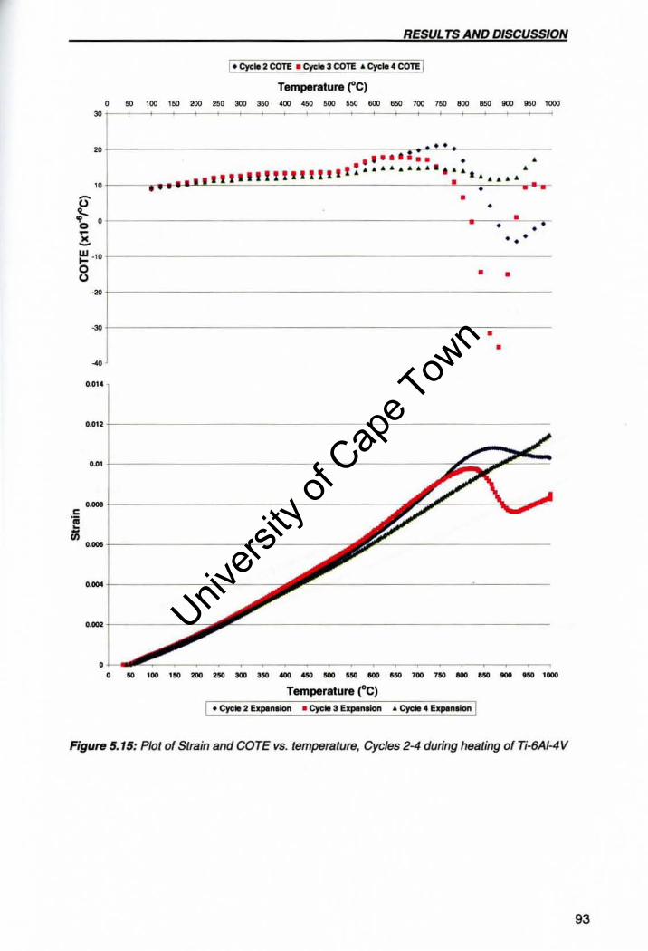
RESUL TS AND DISCUSSION
I. Cycle 2 COTE • Cycle 3 COTE .. Cycle .. COTE I Temperatur. ('C)
• " ,., '" "'" "" "'" "" ... '"
,., ... .. '" ,.,
'" .. ... .., '" ",.,
"
" •• • • • III • i • • • •
, . .............. .. . t .. .. ..
.. -...... . ••• IIIII!!IIIIIII .. • .. H .....
" • r " r - " (J • }- • " 0 " • • • ~ • " •• -~ - 'O 0 " " (J
."
" "
~
0.014
0 .012
~,
•. -c .. --.. .. -0.0.'
... • • .. ,., , .. "" "" ... . .. - '" .. ... ... ... ,., , .. .., ... .., ... ,-
Temperature r C) • c~ .. 2 Expellliorl .. eye .. :5 EllpIInlion ... eyele .. E!I9'nlior! I
Figure 5.15: Plot of Strain and COTE vs. temperature, Cycles 2-4 during heating of Ti-6AI-4V
93
Univers
ity of
Cap
e Tow
n
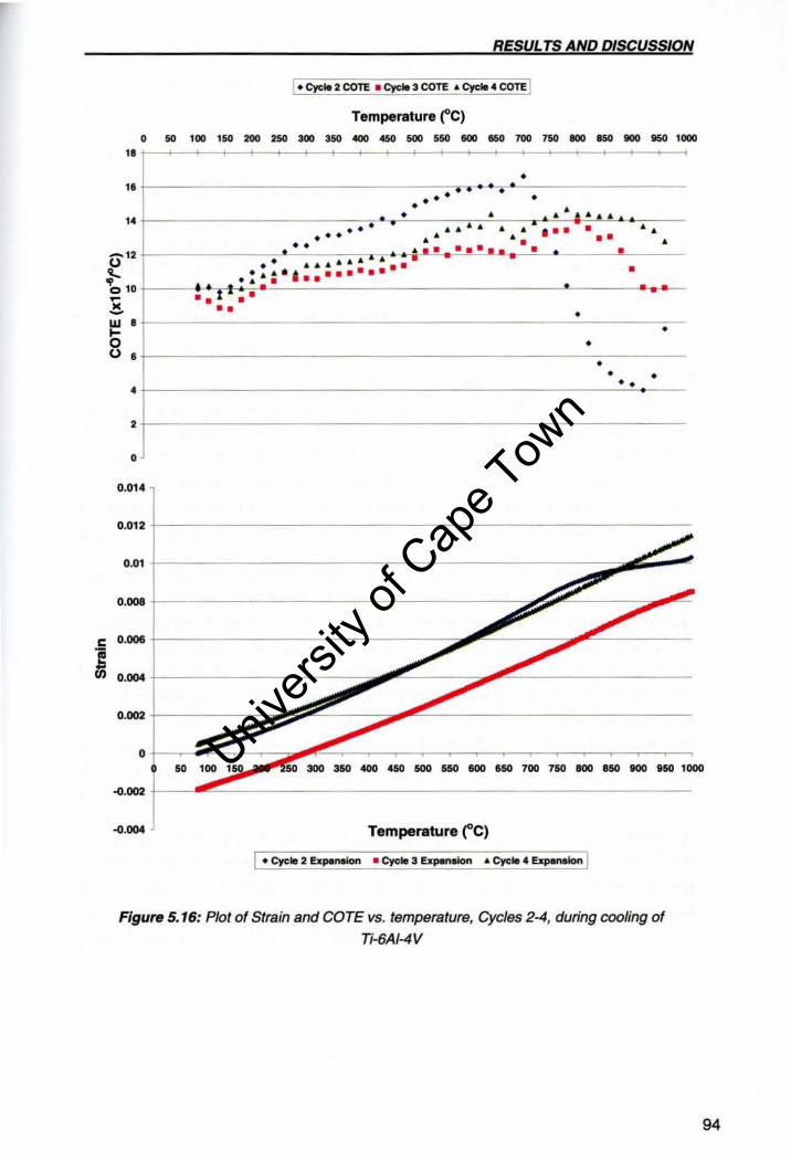
RESUL TS AND DISCUSSION
I. CyW 2 COTE • cya. 3 COTE .. ~ .. 4 COTE I
Temperature r C) 1_.'_. _______________ _ "
• " ..
0' 12 .... ~ 10 ~
.!!.
•• • - +-.. -
• • • • • • • .0. &~&.." -. • • •
. . . .. .. .. .. ... .. ..... .. • " .. .. .. • .. . • . _ ...... ~ • •••• I . .---!---+ . . .. ........ " .. .. • ... .. I ii •••••• IO.. . ••
.-~t-.. .-• • • •• • w • .... • 0 • " • • • •
• ••
, 1
0.014
0.012 t------------------------- --- --
0.01 t-----------------------------------------------------=:~,. .. -=;. .. --I .... t---------------------:
.= 0 .00& +---------------~"."'---_::;;".~-----
~ O'OO·I-----__:::;;~",.'--__:::;;7"""""------
I .... +----~ ~=_"' =----_=",."'------------
1~2~:::::::::=~~ L-:- 100 50 300 350 400 4&0 500 &&0 &00 850 700 750 eoo 8150 too '50 1000
...... j -0.004 Temperature (,C)
I • Cyde 2 &penekIn • Cyde 3 IEJ;~ .. eyc:_ 4 EapanaIon I
Figure 5.16: Plot of Strain and COTE vs. temperature. Cycles 2-4, during cooling of
Ti-6A14V
94
Univers
ity of
Cap
e Tow
n
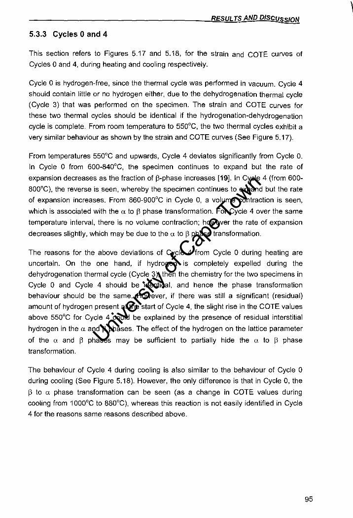
RESUL T5 AND DISCUSSION
5.3.3 Cycles 0 and 4
This section refers to Figures 5.17 and 5.18, for the strain and COTE curves of
Cycles 0 and 4, during heating and cooling respectively.
Cycle 0 is hydrogen-free, since the thermal cycle was performed in vacuum. Cycle 4
should contain little or no hydrogen either, due to the dehydrogenation thermal cycle
(Cycle 3) that was performed on the specimen. The strain and COTE curves for
these two thermal cycles should be identical if the hydrogenation-dehydrogenation
cycle is complete. From room temperature to 550°C, the two thermal cycles exhibit a
very similar behaviour as shown by the strain and COTE curves (See Figure 5.17).
From temperatures 550°C and upwards, Cycle 4 deviates significantly from Cycle O.
In Cycle 0 from 600-840°C, the specimen continues to expand but the rate of
expansion decreases as the fraction of l3-phase increases [19]. In Cycle 4 (from 600-
800°C), the reverse is seen, whereby the specimen continues to expand but the rate
of expansion increases. From 860-900°C in Cycle 0, a volume contraction is seen,
which is associated with the a. to 13 phase transformation. For Cycle 4 over the same
temperature interval, there is no volume contraction; however the rate of expansion
decreases slightly, which may be due to the a. to 13 phase transformation.
The reasons for the above deviations of Cycle 4 from Cycle 0 during heating are
uncertain. On the one hand, if hydrogen is completely expelled during the
dehydrogenation thermal cycle (Cycle 3), then the chemistry for the two specimens in
Cycle 0 and Cycle 4 should be identical, and hence the phase transformation
behaviour should be the same. However, if there was still a significant (residual)
amount of hydrogen present at the start of Cycle 4, the slight rise in the COTE values
above 550°C for Cycle 4 could be explained by the presence of residual interstitial
hydrogen in the a. and 13 phases. The effect of the hydrogen on the lattice parameter
of the a. and 13 phases may be sufficient to partially hide the a. to 13 phase
transformation.
The behaviour of Cycle 4 during cooling is also similar to the behaviour of Cycle 0
during cooling (See Figure 5.18). However, the only difference is that in Cycle 0, the
13 to a. phase transformation can be seen (as a change in COTE values during
cooling from 1000°C to 880°C), whereas this reaction is not easily identified in Cycle
4 for the reasons same reasons described above.
95
Univers
ity of
Cap
e Tow
n
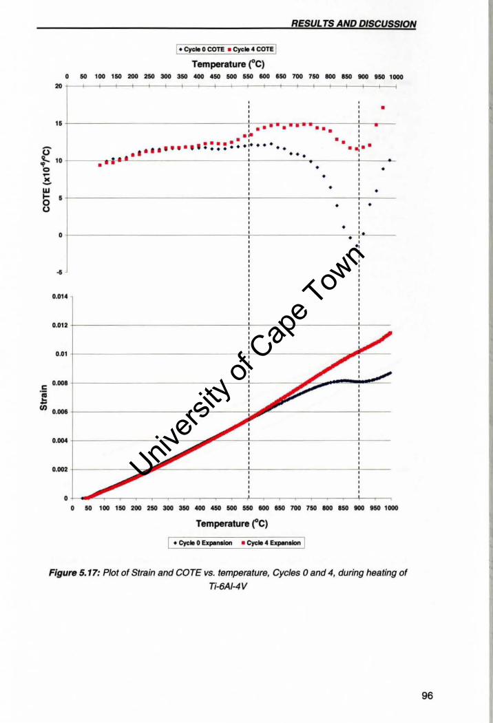
~ -• -W l-0
"
.E e -on
RESUL TS AND DISCUSSION
I_ Cydt 0 COTE • CycII .. COTE I Temperature r C) D.' __________________ ,.
• • • • • • • • • • t---------------------------------------~:Cc.-;.,. ..... ~.,.,.~.-------f---.---"
" •
I
D
~
0.014
0.012
0.01
D."
D."
I."
0.002
•• . . . . . " . •• I.·' · " ··.····~·· .. . . , .. I • "
•
• •• • . .: .. •
• •
• • • •
• •
• •
I "-• .-~----------------------------~--------------------~---~~ D.' __________________ ,.
Temperature ("C)
tCyc"O~ ' Cyc:"4~1IkIn I
Figure 5. 17: Plot of Strain and COTE vs. temperature, Cycles 0 and 4, during heating of Ti·6AI-4V
96
Univers
ity of
Cap
e Tow
n
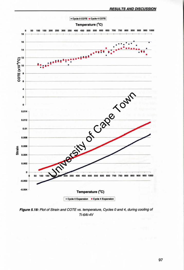
RESUL TS AND DISCUSSION
Temperature (,e) 0.'. ________________ ., • .. .. ---------------------------C7-..-~.'-------. .-• • •• •• • .. t------------------ -----------------::-::-.. ... -:- . • •••••••••• • . ... ' ' .' ... ' . .
0' 12 .... "0 10 ~
• • • .!!. w • .... 0
" • • , 0
0.014
0.012
0.01
0 ...
e 0." e -ili 0."
0."
0
~.'"
~ ... Temperature r C)
Figure 5.18: Plot of Strain and COTE VS. temperature, Cycles a and 4, during cooling of Ti-6Af-4V
97
Univers
ity of
Cap
e Tow
n
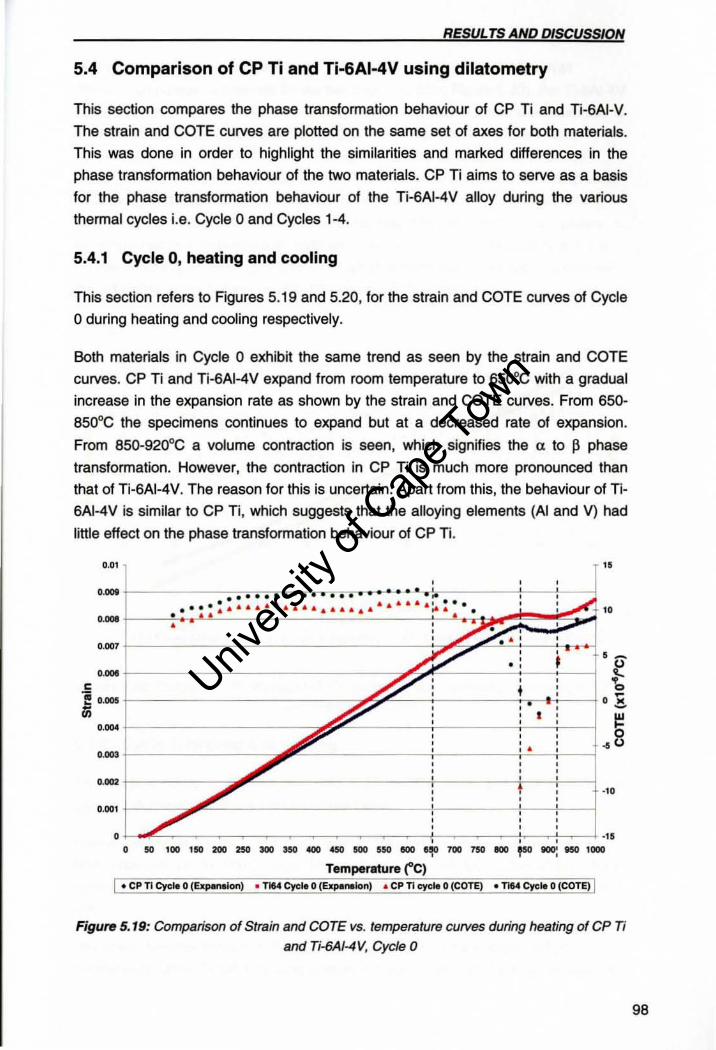
RESUL 15 AND DISCUSSION
5.4 Comparison of CP Ti and Ti-6AI-4V using dilatometry
This section compares the phase transformation behaviour of CP Ti and Ti-SAI-V.
The strain and COTE curves are plotted on the same set of axes for both materials.
This was done in order to highlight the similarities and marked differences in the
phase transformation behaviour of the two materials. CP Ti aims to serve as a basis
for the phase transformation behaviour of the Ti-SAI-4V alloy during the various
thermal cycles Le. Cycle 0 and Cycles 1 ·4.
5.4.1 Cycle 0, heating and cooling
This section refers to Figures 5.19 and 5.20, for the strain and COTE curves of Cycle
o during heating and cooling respectively.
Both materials in Cycle 0 exhibit the same trend as seen by the strain and COTE
curves. CP Ti and Ti-SAI-4V expand from room temperature to 650°C with a gradual
increase in the expansion rate as shown by the strain and COTE curves. From 650~
850°C the specimens continues to expand but at a decreased rate of expansion.
From 850~920°C a volume contraction is seen, which signifies the a to p phase
transformation. However, the contraction in CP Ti is much more pronounced than
that of Ti~6AI~4V. The reason for this is uncertain. Apart from this, the behaviour of Ti~
6AI-4V is similar to CP Ti , which suggests that the alloying elements (AI and V) had
little effect on the phase transformation behaviour of CP Ti.
0.01
.. ""
....
..
.. -----------.---~~-Temperature ("C) I • CP T1 C'yeJ. 0 (bPl.lon) • T164 CycJ. 0 (bPI_ion) • CP TI cytJ. 0 (COTE) • Tl64 CycJt 0 (COTE) I
Figure 5.19: Comparison of Strain and COTE vs. temperature curves during heating of CP Ti
and Ti~6AI-4 V, Cycle 0
98
Univers
ity of
Cap
e Tow
n
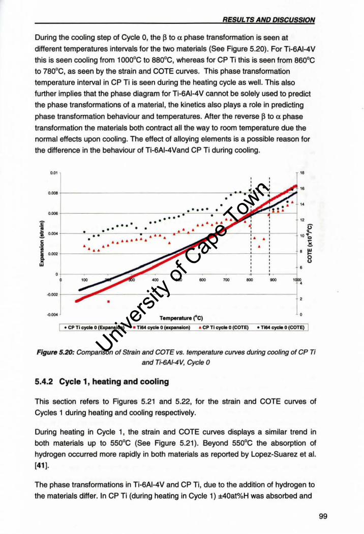
RESULTS AND DISCUSSION
During the cooling step of Cycle D. the p to a phase transformation is seen at
different temperatures intervals for the two materials (See Figure 5.20). For Ti-SAI-4V
this is seen cooling from 1000°C to 8800e, whereas for CP Ti this is seen from 860°C
to 780°C, as seen by the strain and COTE curves. This phase transformation
temperature interval in CP Ti is seen during the heating cycle as well . This also
further implies that the phase diagram for Ti-SAI-4V cannot be solely used to predict
the phase transformations of a material , the kinetics also plays a role in predicting
phase transformation behaviour and temperatures. After the reverse P to a phase
transformation the materials both contract all the way to room temperature due the
normal effects upon cooling. The effect of alloying elements is a possible reason for
the difference in the behaviour of Ti-6AI-4Vand CP Ti during cooling.
0.0\ " .... j---------------:o'~·T"--;!J'~'1 "
, . .... +-------------~r'-'-'O"C_.-'---..
.-. ... -i • • • • • • •• • ! 11.11001 +--~-..-..-'-'---~-.cr •• . -.-'-::""-=--,~~---+--+---j I; • 66666666
£. ..' ' .. J .... 1----=--=-------= w ~~_-LL~ .+-----~~~~
" u "-
10 "0 E
• 5 u
• .. "" .. .. , .. •
. ... +--.:.,.."."""-----------------------1 •
..... Temper.tu,-. (,C) •
• CP TI c)'Cle 0 (ExpM!Ion) I TIM C)'CIe 0 (uplrWon) 6 CP TI cydI 0 (COTE) • TI64 C)'CIe 0 (COTE) I
Figure 5.20: Comparison of Strain and COTE vs. temperature CUNes during cooling of CP Ti
and Ti-6AI-4 V, Cycle 0
5.4.2 Cycle 1, heating and cooling
This section refers to Figures 5.21 and 5.22, for the strain and COTe curves of
Cycles 1 during heating and cooling respectively.
During heating in Cycle 1, the strain and COTe curves displays a similar trend in
both materials up to 550' C (See Figure 5.21). Beyond 550' C the absorption of
hydrogen occurred more rapidly in both materials as reported by Lopez-Suarez et al.
[41 ).
The phase transformations in Ti-6AI-4V and CP Ti, due to the addition of hydrogen to
the materials differ. In CP Ti (during heating in Cycle 1) ±40at%H was absorbed and
99
Univers
ity of
Cap
e Tow
n
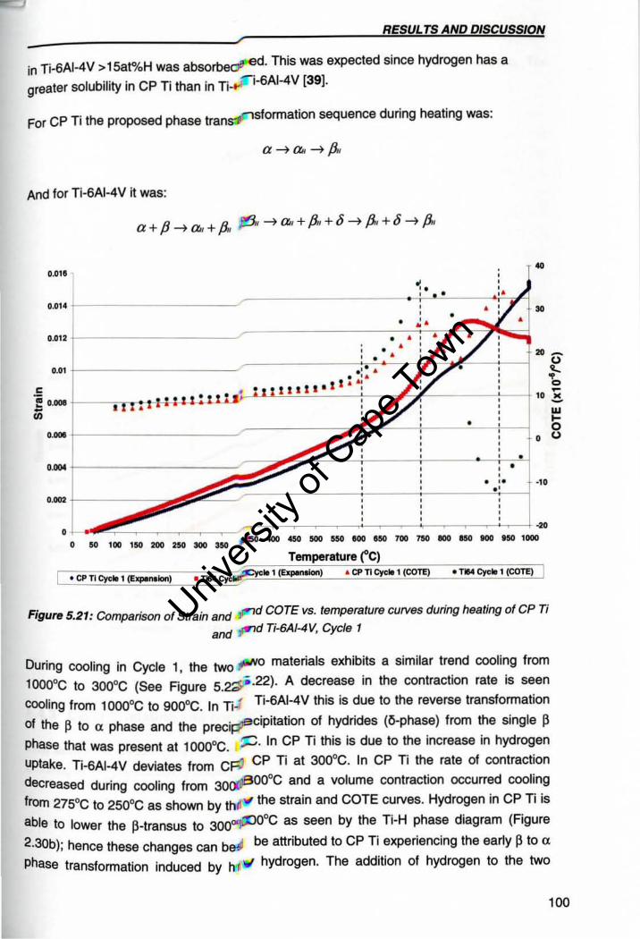
RESUL TS AND DISCUSSION -in Ti-6AI-4V > 15at%H was absorb~d. This was expected since hydrogen has a
greater solubility in CP Ti than in Ti- i-SAI-4V (39).
For CP Ti the proposed phase tran sformation sequence during heating was:
And for Ti-SAI-4 V it was:
0.0111 T" • " , , • " • 0.014 , • .. , • • •• • 0.012
• • • .. -<J , • I ,., .,' " ~ . " c • UIII · IJ " ~ ~ 0.001 :-t-l-:-l-1-1 : : ! : I • " -'" • , ... ,
• , ... , • , • " -" .' ' .002
, -,.------ ~ ------~-----Temperatura re) • CP TI Cydt 1 ~) • TlI4 Cy!:~ .. 1 (ExpMIIonl I Cp n C)'de 1 (COTE) • TIM Cycle 1 (COl'f) I
Figure 5.21: Comparison of Strain snd ~d COTE vs. temperature curves during heating of CP Ti and ,.,d Ti-6AJ.-4 V, Cycle 1
During cooling in Cycle 1, the two JlM'o materials exhibits a similar trend cooling from
lOOaoe to 30Qoe (See Figure 5.2# ·22). A decrease in the contraction rate is seen
COOling from 10OQoC to 900oe. In TiJ Ti-SAI-4V this is due to the reverse transformation
of the ~ to a phase and the precipl"cipitation of hydrides (O-phase) from the single ~ phase that was present at 1 OO00C. ~. In CP Ti this is due to the increase in hydrogen
uptake. Ti-SAI-4V deviates from cF::1 CP Ti at 300' C. In CP Ti the rate of contraction
decreased during cooling from 30()tll800°C and a volume contraction occurred cooling
from 275' C to 250' C as shown by th the strain and COTE curves. Hydrogen in CP Ti is
able to lower the ~-transus to 300,.,:JJO'C as seen by the Ti-H phase diagram (Figure
2.30b); hence these changes can b.,.i be attributed to CP Ti experiencing the early p to a phase transformation induced by M W hydrogen. The addition of hydrogen to the two
C> -" -w >-0 <J
100
Univers
ity of
Cap
e Tow
n
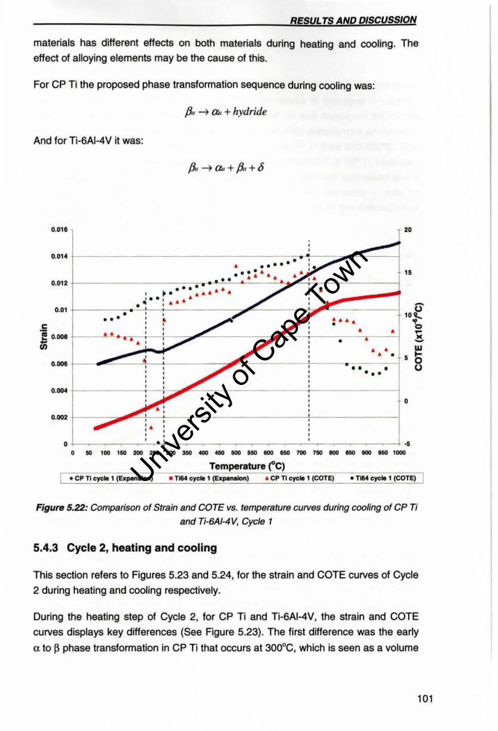
RESULTS AND DISCUSSION
materials has different effects on both materials during heating and cooling. The effect of alloying elements may be the cause of this.
For CP Ti the proposed phase transformation sequence during cooling was:
And for Ti-SAI-4V it was:
0.01'
0.014
0.012
p.. --> a. + hydride
.. .. ...... ... .. .. ' .... .. . . . . .. I ~ • .. .. .... ..
~ .. , ........
r"
"
-0.01 • • • • . ' • I , , , , . , , , , : ...... 10~
c ! 0.008 • Iii
0.'"
'b • • ~
• " -• • '" • • • b •• • u •••
t----"UL.~.__ :--;'--_.~~--------_C~EC--4-----~--.. ---c, . ,
0.""
0
0.002
0_.' ___ '---------------Temperature rC) • CP Tl C:)'C" 1 (&,.,mon) • TIM cycIit, (&~) .. CP Tl c:)'C'" (COTE) • TIM c:ye .. , (COTE)
Figure 5.22: Comparison of Strain and COTE vs. temperature curves during cooling of CP Ti and fi.6AI-4V, Cycle 1
5,4,3 Cycle 2, heating and cooling
This section refers to Figures 5,23 and 5.24, for the strain and COTE curves of Cycle 2 during heating and cooling respectively,
During the heating step of Cycle 2, for CP Ti and Ti-SAI-4V, the strain and COTE
curves displays key differences (See Figure 5.23). The first difference was the earty
a to p phase transformation in CP Ti that occurs at 30QoC, which is seen as a volume
101
Univers
ity of
Cap
e Tow
n
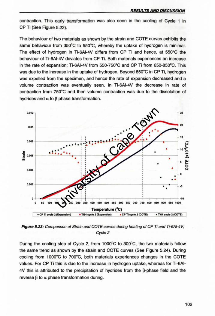
RESUL TS AND DISCUSSION
contraction. This early transformation was also seen in the cooling of Cycle 1 in
CP Ti (See Figure 5.22).
The behaviour of two materials as shown by the strain and COTE curves exhibits the
same behaviour from 350°C to 550°C, whereby the uptake of hydrogen is minimal.
The effect of hydrogen in Ti-6AI-4V differs from CP Ti and hence, at 550'C the
behaviour of Ti-6AI-4V deviates from CP Ti. Both materials experiences an increase
in the rate of expansion; Ti-6AI-4V from 550-750' C and CP Ti from 650-850' C. This
was due to the increase in the uptake of hydrogen. Beyond 850°C in CP Ti, hydrogen
was expelled from the specimen, and hence the rate of expansion decreased and a
volume contraction was eventually seen. In Ti-6AI-4V the decrease in rate of
contraction from 750°C and then volume contraction was due to the dissolution of
hydrides and a to p phase transformation.
0.012 " ,
t--------------------------------~.·~~·t'~~~~~~a .. , . - . • • ..
• • , , . , , : .... " , . .,. i---------------:---;--::.: :. 'f".-:-.-.....-I,....,'-=-'O"" ... -.;JjIF>-',"-"-c,,--~-----1 ••••• t , .. " ... •
• 10 'b • ~ .... .. - " "" ' ..
• ~ 0.001 +------=..::...:'-'-''---:...:.~-:...;..----------c __ '---..~--+_----------__1 o •
• • • • 0 .... +----------------: . ..;..~ __ "--'I;c..----------+_----------'-__1
0 • • ..
0.002 i-----------... ~ -;.""'''--------------------:-------;.;-,~_i ~ •
o ., -10 ,--------------------Temperature ("C) I • cp n era- 2 (bpMelDn) • T1I4 eye .. 2~) .. cp n cycM 2 (COTE)
Figure 5.23: Comparison of Strain and COTE CUfV8S during heating of CP Ti and Ti-6AI-4 V,
Cyc/e2
-" -w .... 0 <.>
During the cooling step of Cycle 2, from 1000°C to 300°C, the two materials follow
the same trend as shown by the strain and COTE curves (See Figure 5.24). During
cooling from 1000°C to 700°C, both materials experiences changes in the COTE
values. For CP Ti this is due to the increase in hydrogen uptake, whereas for Ti-6AI-
4V this is attributed to the precipitation of hydrides from the ~-phase field and the
reverse ~ to a phase transfonnation during.
102
Univers
ity of
Cap
e Tow
n
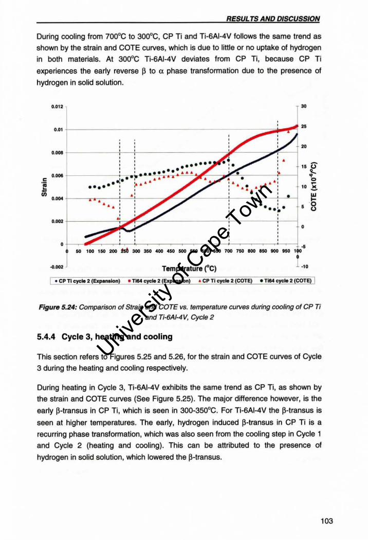
RESUL TS AND DISCUSSION
During cooling from 7000e to 3000e, CP Ti and Ti-6AI-4V follows the same trend as
shown by the strain and COTE curves, which is due to little or no uptake of hydrogen
in both materials. At 300°C Ti-6AI-4V deviates from CP Ti, because CP Ti
experiences the early reverse p to a phase transformation due to the presence of
hydrogen in solid solution.
0.012 r +----------- --------::------::::;;;00...,.."":: " 0.01 I
, , , . , , , , .. .. " ,
.10 .. . ...... , .. : , . ' •••••
20
15 U }-C> -10 ~
S • u
. k~~::::=-~~~--;-~~, i,---.-----j · ·1·-- ~---- ----_-----,r4
Temperature re) -10
• cp n eye. 2 ~) • TIM cycle 2 (EKpwIon) .. CP TI eyele 2 (COTE) • Tl84 cycle 2 (COTE) I
Figure 5.24: Comparison of Strain and COTE vs. temperature curves during cooling of CP Ti
and Ti-6Af-4V, Cycle 2
5.4.4 Cycle 3, heating and cooling
This section refers to Figures 5.25 and 5.26, for the strain and COTE curves of Cycle
3 during the heating and cooling respectively.
During heating in Cycle 3, Ti-6AI-4V exhibits the same trend as CP Ti , as shown by
the strain and COTE curves (See Figure 5.25). The major difference however, is the
early ~-transus in CP Ti, which is seen in 300-350°C. For Ti-SAI-4V the ~-transus is
seen at higher temperatures. The early, hydrogen induced ~-transus in CP Ti is a
recurring phase transformation, which was also seen from the cooling step in Cycle 1
and Cycle 2 (heating and cooling). This can be attributed to the presence of
hydrogen in solid solution, which lowered the ~-transus.
103
Univers
ity of
Cap
e Tow
n
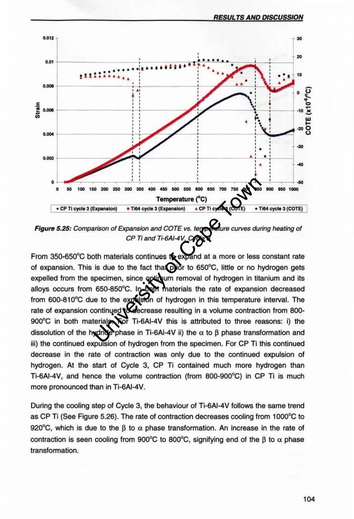
RESUL TS AND DISCUSSION
0.012 .. ,.
0.01 t-------~-:-:j;_;__;_;_;_;lfil ... _.:~·~-'-·-'-·~ .. ~ .. ;t- j_-_j . .... ~ •••• , .t t . · ~ '. . .. .. .. .., I .. III ........ ' '
.. I : :
O.w t--------------~·-----------T~~~~~t-~~~ , .'
•• I 10 • • -0 , : , ,
..E ' ,
, 0 , ~ , -~ O.ooe • • +-----------~-----~~~-----~~--4 ·10 I(
Ui : : , , , • , -~ W ....
." 0 0.'" t---------------;---;---:;;;~'__:;",.'-----~----------:_' ... -"'"'i 0
• ..,
..,0' t----------: • • ...
I o ~
0.'. ___ ---------------Temperature (,C) .. cp n cycle 3 (Exptinalon) • TIM cycle 3 (Explnak)n) .. CP T1 cycle 3 (COTE) .. TI54 ~ 3 (COTE) I
Figure 5.25: Comparison of Expansion and COTE vs. temperature curves during heating of
CP Ti and fi.6AI-4V, Cycle 3
From 350-650°C both materials continues to expand at a more or less constant rate
of expansion. This is due to the fact that prior to 6S0oe. little or no hydrogen gets
expelled from the specimen, since optimum removal of hydrogen in titanium and its
alloys occurs from 6Sa-eSOoe . In both materials the rate of expansion decreased
from 600-810°C due to the expulsion of hydrogen in this temperature interval. The
rate of expansion continued to decrease resulting in a volume contraction from 800-
900°C in both materials. For Ti-SAI-4V this is attributed to three reasons: i) the
dissolution of the hydride phase in TI-SAI-4V ii} the a to p phase transformation and
iii) the continued expulsion of hydrogen from the specimen. For CP Ti this continued
decrease in the rate of contraction was only due to the continued expulsion of
hydrogen. At the start of Cycle 3, CP Ti contained much more hydrogen than
Ti-SAI-4V, and hence the volume contraction (from 800-900°C) in CP Ti is much
more pronounced than in Ti-SAI-4V.
During the cooling step of Cycle 3, the behaviour of Ti-6AI-4V follows the same trend
as CP Tl (See Figure 5.2S). The rate of contraction decreases cooling from 1000°C to
920°C, which is due to the p to a phase transformation. An increase in the rate of
contraction is seen cooling from 900°C to 800°C, signifying end of the p to a phase
transformation.
104
Univers
ity of
Cap
e Tow
n
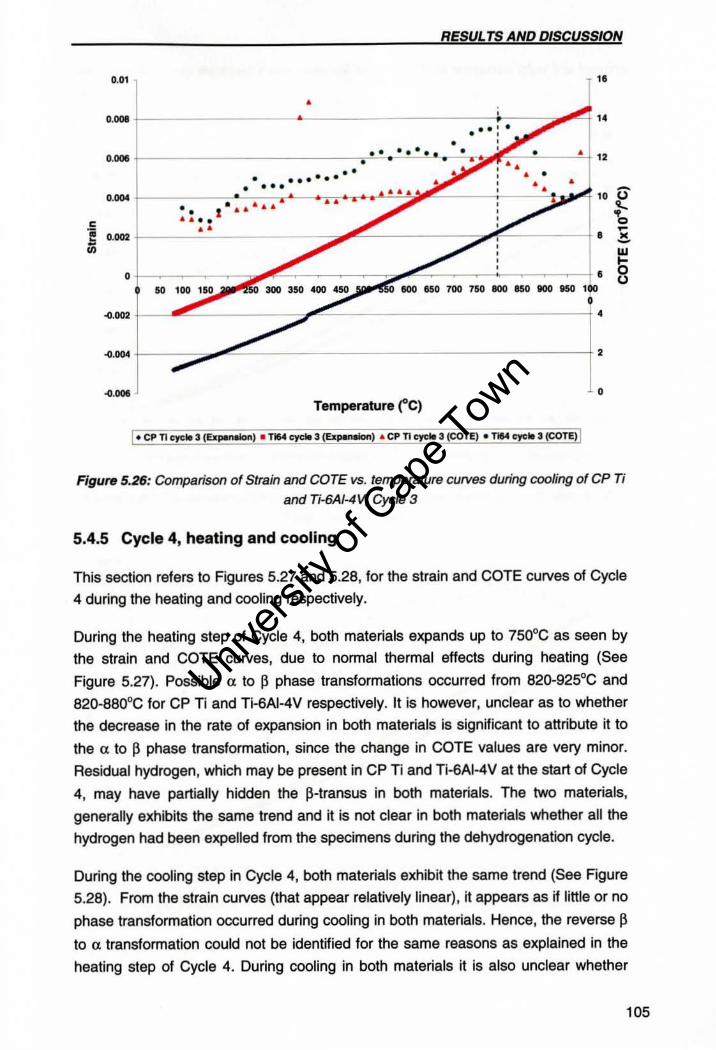
0.01
D.'"
D.'"
0.00'
c
~ 0.00'
0
".002
... '"
... ".
RESUL TS AND DISCUSSION
• I" +-----------------~--------------------~----~--~ "
• .~~--'----__'_l. "
• • ••••••• • •••• }-________ ~~--~--_.~~~~~~~----~---~~~~10 jJ .. S······ -.... .. b
.' -t-----~~------------~~~----------~~~------_+ . ~ w ...
t-~~~..---, ~""-.-~~~- .. ~:,-~~.:,-~~..--f ' 8 IlOO 650 700 750 100 150 IlOO MO 1 \KI
~~~:.-------~~~----------------------+ ,
+-----~~~----------------------------------_4 ,
o Temperature rC)
I_ cp n qde 3 (EJ:panMIn) • 1164 qrctI 3~) .. cp n qoc .. 3 (COTE) • TIM c)'C1e 3 (COTE) I
Figure 5.26: Comparison of Strain and COTE vs. temperature curves during cooling of CP Ti
and Ti-6AI-4V. Cycle 3
5.4.5 Cycle 4, heating and cooling
This section refers to Figures 5.27 and 5.28, for the strain and COTE curves of Cycle
4 during the heating and cooling respectively.
During the heating step of Cycle 4, both materials expands up to 750°C as seen by
the strain and COTE curves, due to normal thermal effects during heating (See
Figure 5.27). Possible a to ~ phase transformations occurred from 820-92SoC and
820-880°C for CP Ti and Ti-SAI-4V respectively. It is however, unclear as to whether
the decrease in the rate of expansion in both materials is significant to attribute it to
the a to p phase transformation, since the change in COTE values are very minor.
Residual hydrogen, which may be present in CP Ti and Ti·6AI·4V at the start of Cycle
4, may have partially hidden the p-transus in both materials. The two materials,
generally exhibits the same trend and it is not clear in both materials whether all the
hydrogen had been expelled from the specimens during the dehydrogenation cycle.
During the cooling step in Cycle 4, both materials exhibit the same trend (See Figure
5.28). From the strain curves (that appear relatively linear), it appears as if little or no
phase transformation occurred during cooling in both materials. Hence, the reverse p
to a transformation could not be identified for the same reasons as explained in the
heating step of Cycle 4. During cooling in both materials it is also unclear whether
105
Univers
ity of
Cap
e Tow
n
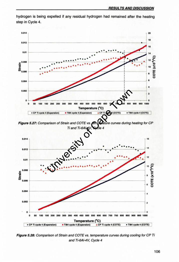
RESUL TS AND DISCUSSION
hydrogen is being expelled if any residual hydrogen had remained after the heating
step in Cycle 4.
0.0" " " 0.012 1_-----------------------------.---1
" .. . .. .. 0.01 1_-----------------.~-'--'-"--'-'-'--~ ... ,;__::> ... "'--=--___i
" •• -• U
• 12 -t . .. . . . .. .
C• · .. 1---------,-,.-.-. • • • • • .~...,'---• .;"'---::. ... "!--'--- .,_'y . .. . ... .. .. . . ..... .. ~
.5 • • .. • ....... " • -~0.~ 1_---C~-r'~·'------------~~~,,~--~-----~ •• • ~
U ..... !-------------,.,.,.s.,...."----------!------{ •
• .... j-------:: ,
• Temperature rC)
.cpncp4~) • cp n qo$ .. (COTE) • TIM qo$ .. (COTE)
Figure 5.27: Comparison of Strain and COTE vs. temperature cUlVes during heating for CP
Ti and Ti-6AI-4V. Cycle 4
o.Ot ..
• + __________________ .. "".-·"'-.,.c·O-·_·_·_·_·~·"·'"~__l 0.012 • • •
• • • •••
t--------c~c' .~L<,.c·c·'--------_c.c~--~.,., 0.0, . -. . .. . . ..
.. "
" -•• • •• • •••••••••••••••••• .. u ~ 0 ~ • .!!. I!!
. ...... C 0.008 +-__ ... ..:...'-'--=-'-0-____________ --::;.;"'-- .... -"''----, •
~ VI 0.008 +------------------o,,"'-.... """=-----------l
• 0 U
..... +--------------: •
..... +--------o .. ~"--------------------___i ,
• • o 50 100 150 200 250 300 350 400 .. 50 500 550 500 HO 700 750 100 850 100 MO tooo
Tern .ture C .. CP T1 eye .. 4 (Eq)lMIon) • CP T1 eye .. 4 (COTE) • TIM tycIe 4 (COTE)
Figure 5.28: Comparison of Strain and COTE vs. temperature cUlVes during cooling for CP Ti
and Ti-6AI-4V. Cycle 4
t06
Univers
ity of
Cap
e Tow
n
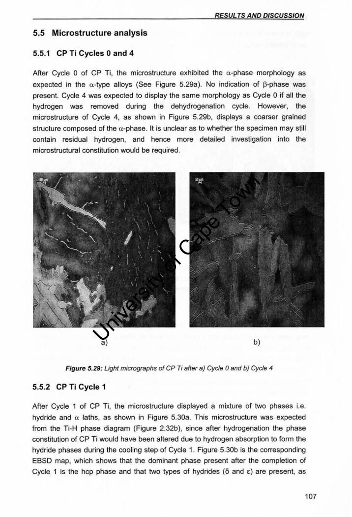
RESULTS AND DISCUSSION
5.5 Microstructure analysis
5.5.1 CP Ti Cycles 0 and 4
After Cycle 0 of CP Ti, the microstructure exhibited the a-phase morphology as
expected in the a-type alloys (See Figure 5.29a). No indication of J3-phase was
present. Cycle 4 was expected to display the same morphology as Cycle 0 if all the
hydrogen was removed during the dehydrogenation cycle. However, the
microstructure of Cycle 4, as shown in Figure 5.29b, displays a coarser grained
structure composed of the a -phase. It is unclear as to whether the specimen may still
contain residual hydrogen, and hence more detailed investigation into the
microstructural constitution would be required.
a) b)
Figure 5.29: Light micrographs of CP Ti after a) Cycle 0 and b) Cycle 4
5.5.2 CP Ti Cycle 1
After Cycle 1 of CP Ti, the microstructure displayed a mixture of two phases i.e.
hydride and Cl laths, as shown in Figure 5.30a. This microstructure was expected
from the Ti-H phase diagram (Figure 2.32b), since after hydrogenation the phase
constitution of CP Ti would have been altered due to hydrogen absorption to form the
hydride phases during the cooling step of Cycle 1. Figure 5.30b is the corresponding
EBSD map, which shows that the dominant phase present after the completion of
Cycle 1 is the hcp phase and that two types of hydrides (6 and £) are present, as
107
Univers
ity of
Cap
e Tow
n
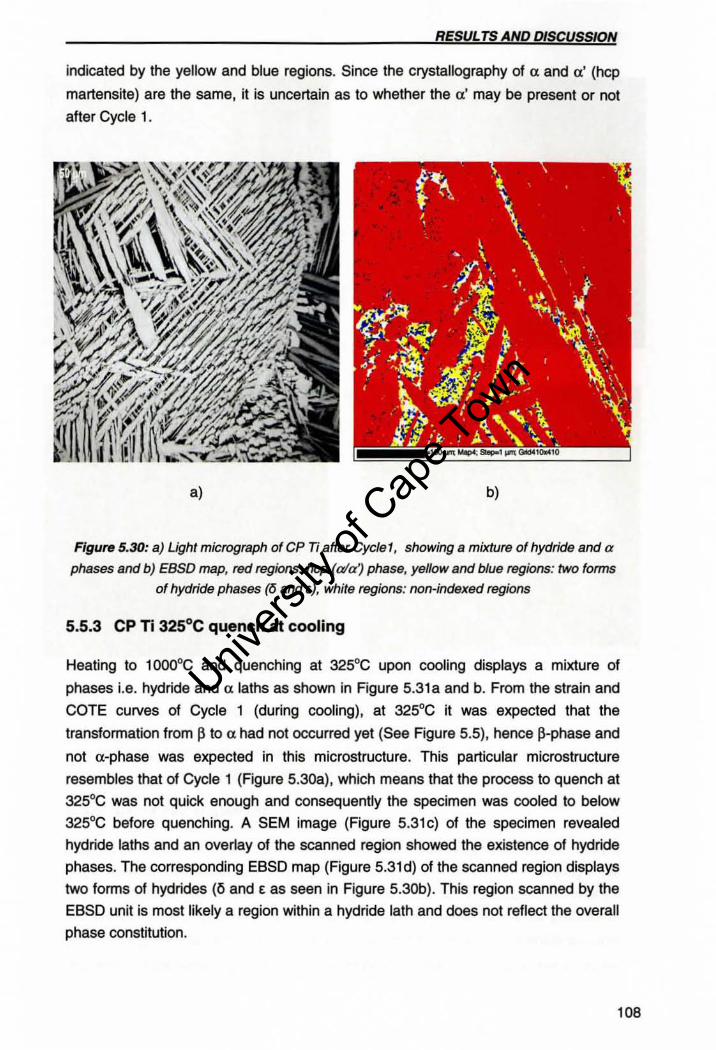
RESUL TS AND DISCUSSION
indicated by the yellow and blue regions. Since the crystallography of a and a' (hcp
martensite) are the same, it is uncertain as to whether the (J,' may be present or not
after Cycle 1.
a) b)
Figure 5.30: a) Light micrograph of CP Ti after eyelel, showing a mixture of hydride and a
phases and b) EBSD map, red regions: hcp (ala') phase, yellow and blue regions: two fonns
of hydride phases (6 and t). white regions: non-indexed regions
5.5.3 CP Ti 325'C quench at cooling
Heating to 100QoC and quenching at 325°C upon cooling displays a mixture of
phases i.e. hydride and a laths as shown in Figure 5.31a and b. From the strain and
COTE curves of Cycle 1 (during cooling), at 325'C it was expected that the
transformation from p to a had not occurred yet (See Figure 5.5), hence p-phase and
not a-phase was expected in this microstructure. This particular microstructure
resembles Ihat of Cycle 1 (Figure 5.30a), which means that the process to quench at
325°C was not quick enough and consequently the specimen was cooled to below
325°C before quenching. A SEM image (Figure 5.31c) of the specimen revealed
hydride laths and an overlay of the scanned region showed the existence of hydride
phases. The corresponding EBSD map (Figure 5.31 d) of Ihe scanned region displays
two forms of hydrides (l'l and £ as seen in Figure 5.30b). This region scanned by the
EBSD unit is most likely a region within a hydride lath and does not reflect the overall
phase constitution.
108
Univers
ity of
Cap
e Tow
n
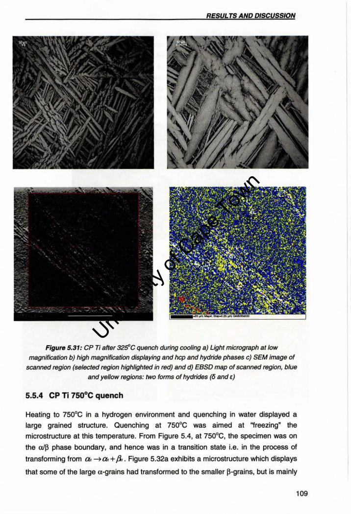
RESULTS AND DISCUSSION
Figure 5.31: CP Ti after 32S'C quench during cooling a) Ught micrograph at low
magnification b) high magnification displaying and hcp and hydride phases c) SEM image of
scanned region (selected region highlighted in red) and d) EBSD map of scanned region, blue
and yellow regions: two forms of hydrides (~ and £)
5.5.4 CP Ti 7SOoC quench
Heating to 750°C in a hydrogen environment and quenching in water displayed a
large grained structure. Quenching at 750°C was aimed at "freezing" the
microstructure at this temperature. From Figure 5.4, at 750°C, the specimen was on
the aIf3 phase boundary, and hence was in a transition state i.e. in the process of
transforming from a, ~ a, + ~ . Figure 5.328 exhibits a microstructure which displays
that some of the large a.-grains had transformed to the smaller p-grains, but is mainly
109
Univers
ity of
Cap
e Tow
n

RESUL TS AND DISCUSS/ON
composed the large a-grains. The scanned region from the SEM and EBSD images
(Figures 5.32b and c) shows that quenching from 750' C resulted in a mixture of hcp
(either the" or "') and two forms of hydrides (~ and E) dispersed within the hcp
phase. Hydrides were not expected to be present at room temperature, since
quenching at 750°C was meant to "freeze- the microstructure at this temperature.
This suggests that the cooling rate during quenching was not fast enough in order to
"freeze" the microstructure, and hence the precipitation of hydrides occurred during
cooling.
a)
b) c)
Figure 5.32: CP Ti after 7sCfc quench a) Light micrograph at /ow magnification displaying
large a-grains and smaller p-grains b) SEM image of scanned region (selected region
highlighted in red) and c) EB5D map of scanned region, red region: hcp phase (aid), yel/ow
and blue regions: two forms of hydrides (~ and £)
110
Univers
ity of
Cap
e Tow
n
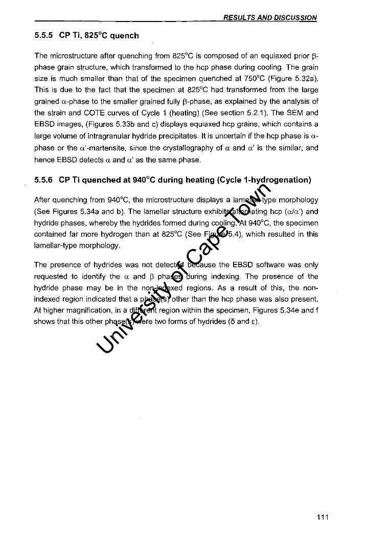
RESUL TS AND DISCUSSION
5.5.5 CP Ti, 825°C quench
The microstructure after quenching from 825°C is composed of an equiaxed prior ~
phase grain structure, which transformed to the hcp phase during cooling. The grain
size is much smaller than that of the specimen quenched at 750°C (Figure 5.32a).
This is due to the fact that the specimen at 825°C had transformed from the large
grained a-phase to the smaller grained fully ~-phase, as explained by the analysis of
the strain and COTE curves of Cycle 1 (heating) (See section 5.2.1). The SEM and
EBSD images, (Figures 5.33b and c) displays equiaxed hcp grains, which contains a
large volume of intragranular hydride precipitates. It is uncertain if the hcp phase is a
phase or the a'-martensite, since the crystallography of a and a' is the similar, and
hence EBSD detects a and a' as the same phase.
5.5.6 CP Ti quenched at 940°C during heating (Cycle 1-hydrogenation)
After quenching from 940°C, the microstructure displays a lamellar-type morphology
(See Figures 5.34a and b). The lamellar structure exhibits alternating hcp (a/a') and
hydride phases, whereby the hydrides formed during cooling. At 940°C, the specimen
contained far more hydrogen than at 825°C (See Figure 5.4), which resulted in this
lamellar-type morphology.
The presence of hydrides was not detected because the EBSD software was only
requested to identify the a and ~ phases during indexing. The presence of the
hydride phase may be in the non-indexed regions. As a result of this, the non
indexed region indicated that a phase(s) other than the hcp phase was also present.
At higher magnification, in a different region within the specimen, Figures 5.34e and f
shows that this other phase(s) were two forms of hydrides (0 and E).
111
Univers
ity of
Cap
e Tow
n
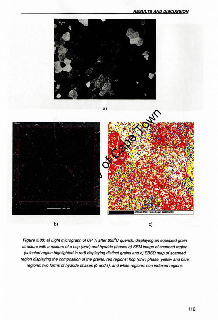
RESULTS AND DISCUSSION
a)
b) c)
Figure 5.33: a) Ught micrograph of CP Ti after 82~C quench, displaying an equiaxed grain
structure with a mixture of a hcp (ala') and hydride phases b) SEM image of scanned region
(selected region highlighted in red) displaying distinct grains and c) EBSD map of scanned
region displaying the composition of the grains, red regions: hcp (a/a') phase, yellow and blue
regions: two forms of hydride phases (6 and e), and white regions: non indexed regions
112
Univers
ity of
Cap
e Tow
n
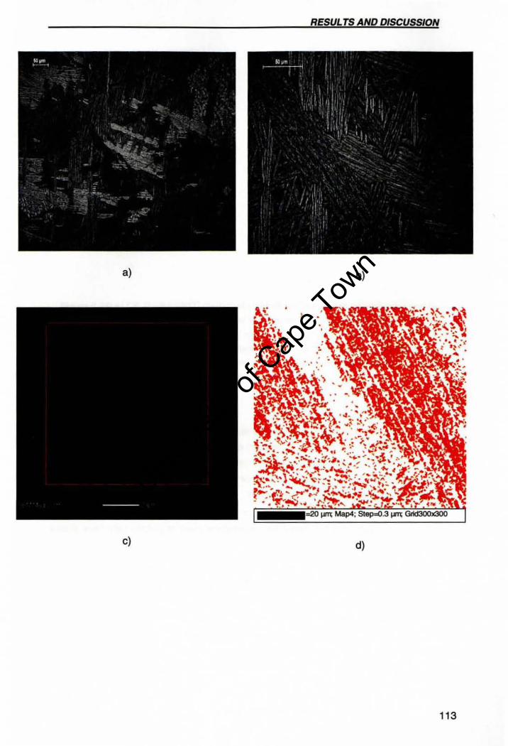
RESUL TS AND DISCUSSION
a) b)
c) d)
113
Univers
ity of
Cap
e Tow
n
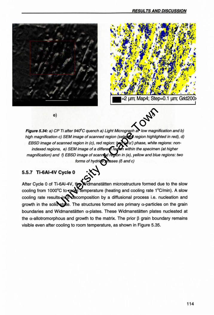
RESUL TS AND DISCUSSION
e) f)
Figure 5.34: a) CP Ti aftsr 94ti'C quench a) Light Micrograph at low magnification and b)
high magnification c) SEM image of scanned region (selected region highlighted in red), d)
EBSD image of scanned region in (e), red region: hcp (a/u) phase, white regions: non
indexed regions, e) SEM image of a different region within the specimen (at higher
magnification) and f) EBSD image of scanned region in (e), yellow and blue regions: two
forms of hydride phases (6 and t.)
5.5.7 Ti-6AI-4V Cycle 0
After Cycte 0 of Ti-6AI-4V, the Widmanstalten microstructure fanned due to the slow
cooling from 1 aoooc to room temperature (heating and cooling rate 1°C/min). A slow
cooling rate results in ~ decomposition by a diffusional process i.e. nucleation and
growth in the solid state. The structures formed are primary a·particles on the grain
boundaries and Widmanstatten a-plates. These Widmanstatten plates nucleated at
the a-allotromorphous and growth to the matrix. The prior p grain boundary remains
visible even after cooling to room temperature, as shown in Figure 5.35.
114
Univers
ity of
Cap
e Tow
n
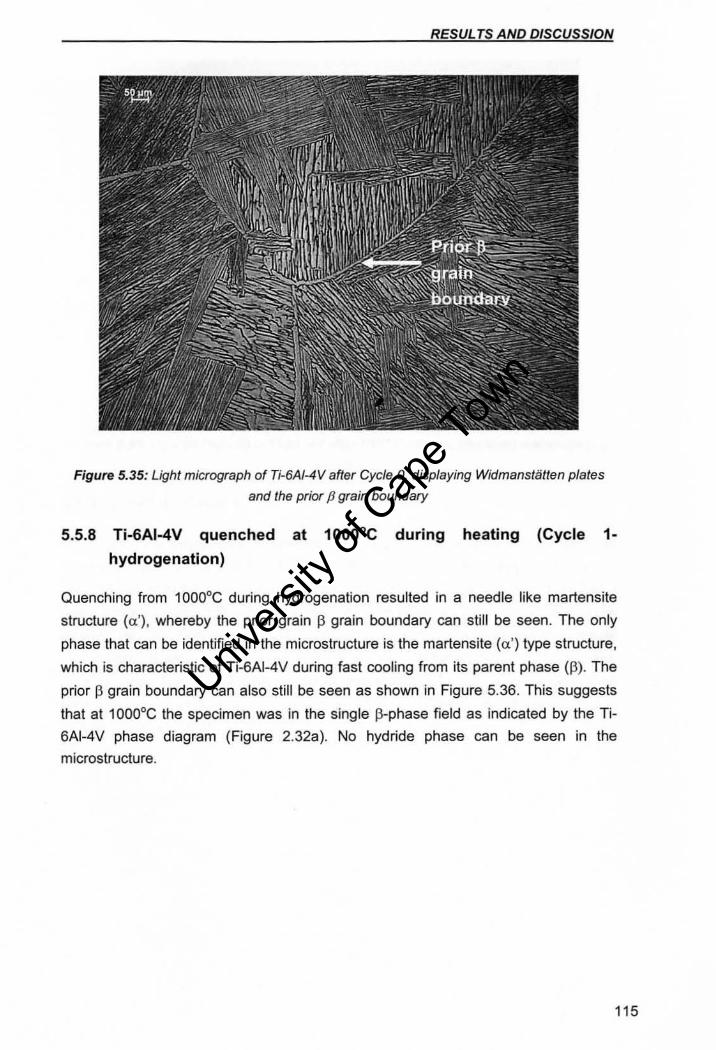
RESULTS AND DISCUSSION
Figure 5.35: Light micrograph of Ti-6A/-4V after Cycle 0, displaying Widmanstatten plates
and the prior p grain boundary
5.5.8 Ti-SAI-4V quenched at 1000·C during heating (Cycle 1-
hydrogenation)
Quenching from 1 DOOoC during hydrogenation resulted in a needle like martensite
structure (a'), whereby the prior grain f3 grain boundary can still be seen. The only
phase that can be identified in the microstructure is the martensite (a') type structure,
which is characteristic of Ti-6AI-4V during fast cooling from its parent phase (13). The
prior (3 grain boundary can also still be seen as shown in Figure 5.36. This suggests
that at 100QoC the specimen was in the single (3-phase field as indicated by the Ti-
6AI-4V phase diagram (Figure 2.32a). No hydride phase can be seen in the
microstructure.
115
Univers
ity of
Cap
e Tow
n
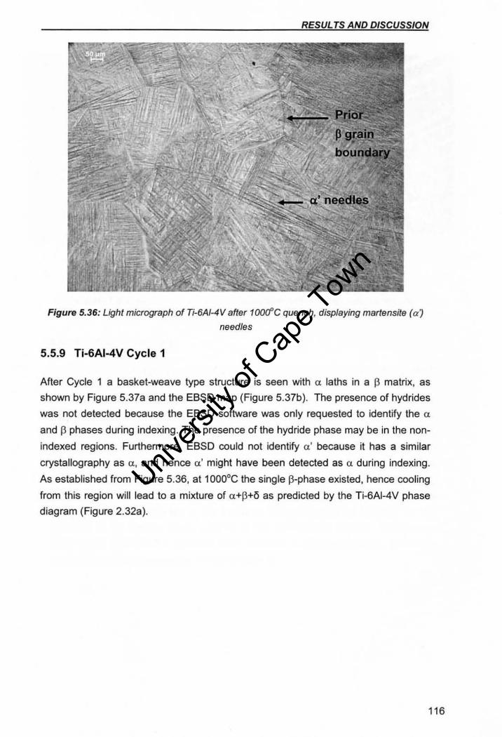
RESULTS AND DISCUSSION
Figure 5.36: Light micrograph of Ti-6AI-4Vafter 10()(fC quench, displaying martensite (a J
needles
5.5.9 Ti-6AI-4V Cycle 1
After Cycle 1 a basket-weave type structure is seen with (l laths in a 13 matrix, as
shown by Figure 5.37a and the EBSD map (Figure S.37b). The presence of hydrides
was not detected because the EBSD software was only requested to identify the (l
and 13 phases during indexing. The presence of the hydride phase may be in the non
indexed regions. Furthermore, EBSD could not identify a' because it has a similar
crystallography as a , and hence a ' might have been detected as a during indexing.
As established from Figure 5.36, at 10000 C the single j3-phase existed. hence cooling
from this region will lead to a mixture of a+I3+i5 as predicted by the Ti-6AI-4V phase
diagram (Figure 2.32a).
116
Univers
ity of
Cap
e Tow
n
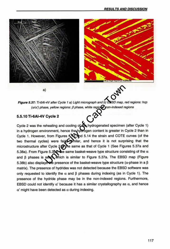
RESULTS AND DISCUSSION
a) b)
F;gure 5.37: Ti·6AI-4V after Cycle 1 a) Ught micrograph and b) EBSD map, red regions: hcp
(a/a') phase, yellow regions: p phase, whffe regions: non-indexed regions
5.5.10 THjAI-4V Cycle 2
Cycle 2 was the reheating and cooling 01 the hydrogenated specimen (alter Cycle 1)
in a hydrogen environment, hence the hydrogen content is greater in Cycle 2 than in
Cycle 1. However, from Figures 5.13 and 5.14 the strain and COTE curves (of the
two thermal cycles) were fairly similar, and hence it is not surprising that the
microstructure after Cycle 2 is the same as that of Cycle 1 (See Figures 5.378 and
5.38a). From Figure S.38a, the same basket-weave type structure consisting of the a
and p phases is seen, which is similar to Figure 5.37a. The EBSD map (Figure
5.38b) also displays the presence of the basket-weave type structure (a-phase in a ~
matrix). The presence of hydrides was not detected because the EBSD software was
only requested to identify the a and ~ phases during indexing (as in Cycle 1). The
presence of the hydride phase may be in the non-indexed regions. Furthermore,
EBSD could not identify a' because it has a similar crystallography as a, and hence
a' might have been detected as a during indexing.
117
Univers
ity of
Cap
e Tow
n
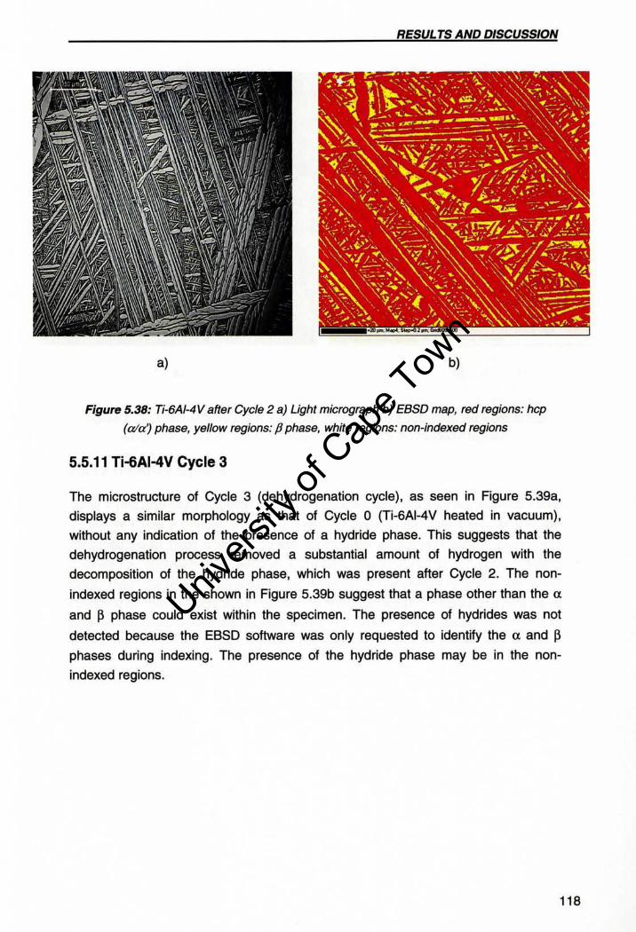
RESUL TS AND DISCUSSION
a) b)
Figure 5.38: Ti·6AI-4V after Cycfe 2 a) Light micrograph b) EBSD map, red regions: hcp
(aid) phase, yelfow regions: P phase, white regions: non-indexed regions
5.5.11 Ti-6AI-4V Cycle 3
The microstructure of Cycle 3 (dehydrogenation cycle), as seen in Figure 5.39a,
displays a similar morphology as that of Cycle 0 (Ti-6AI-4V heated in vacuum),
without any indication of the presence of a hydride phase. This suggests that the
dehydrogenation process removed a substantial amount of hydrogen with the
decomposition of the hydride phase, which was present after Cycle 2. The non
indexed regions in the shown in Figure 5.39b suggest that a phase other than the (X
and p phase could exist within the specimen. The presence of hydrides was not
detected because the EBSD software was only requested to identify the a and ~
phases during indexing. The presence of the hydride phase may be in the non
indexed regions.
118
Univers
ity of
Cap
e Tow
n
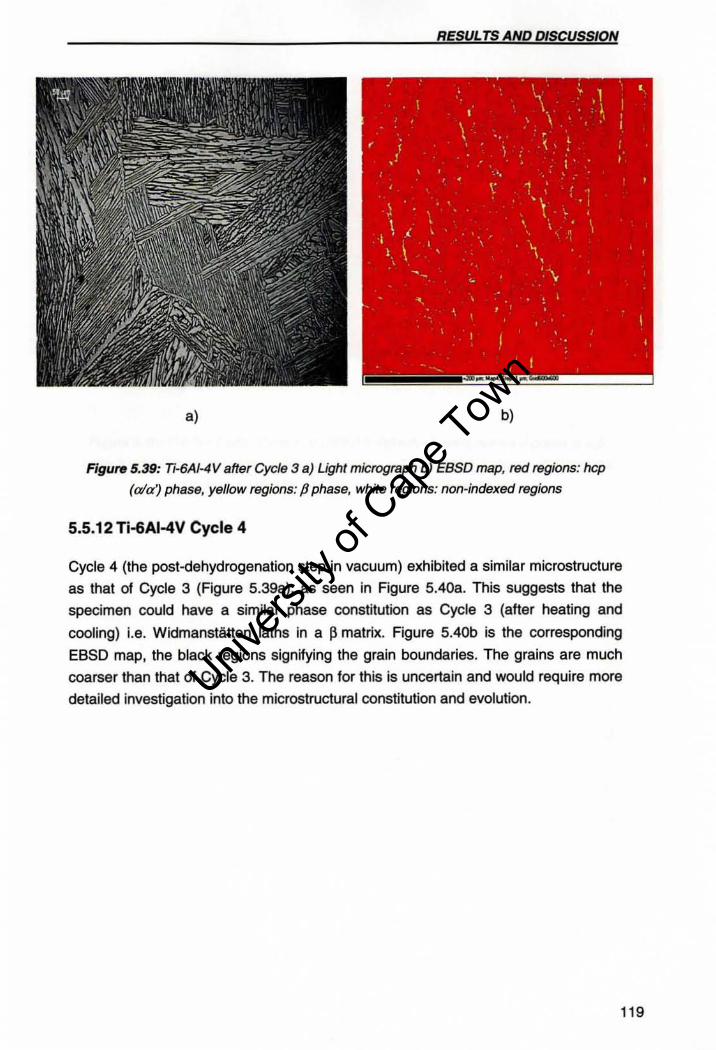
RESUL TS AND DISCUSSION
a) b)
Figure 5.39: Ti·6AI-4Vaftsr Cycle 3 a) Ught micrograph b) EBSD map. red regions: hcp
(ala') phase, yellow regions: P phase, white regions: non-indexed regions
5.5.12 Ti-6AI-4V Cycle 4
Cycle 4 (the post-dehydrogenation step in vacuum) exhibited a similar microstructure
as that of Cycle 3 (Figure 5.39a). as seen in Figure 5.40a. This suggests that the
specimen CQuid have a similar phase constitution as Cycle 3 (after heating and
cooling) i.e. Widmanstatten laths in a p matrix. Figure 5.40b is the corresponding
EBSD map, the black regions signifying the grain boundaries. The grains are much
coarser than that of Cycle 3. The reason for this is uncertain and would require more
detailed investigation into the microstructural constitution and evolution.
119
Univers
ity of
Cap
e Tow
n
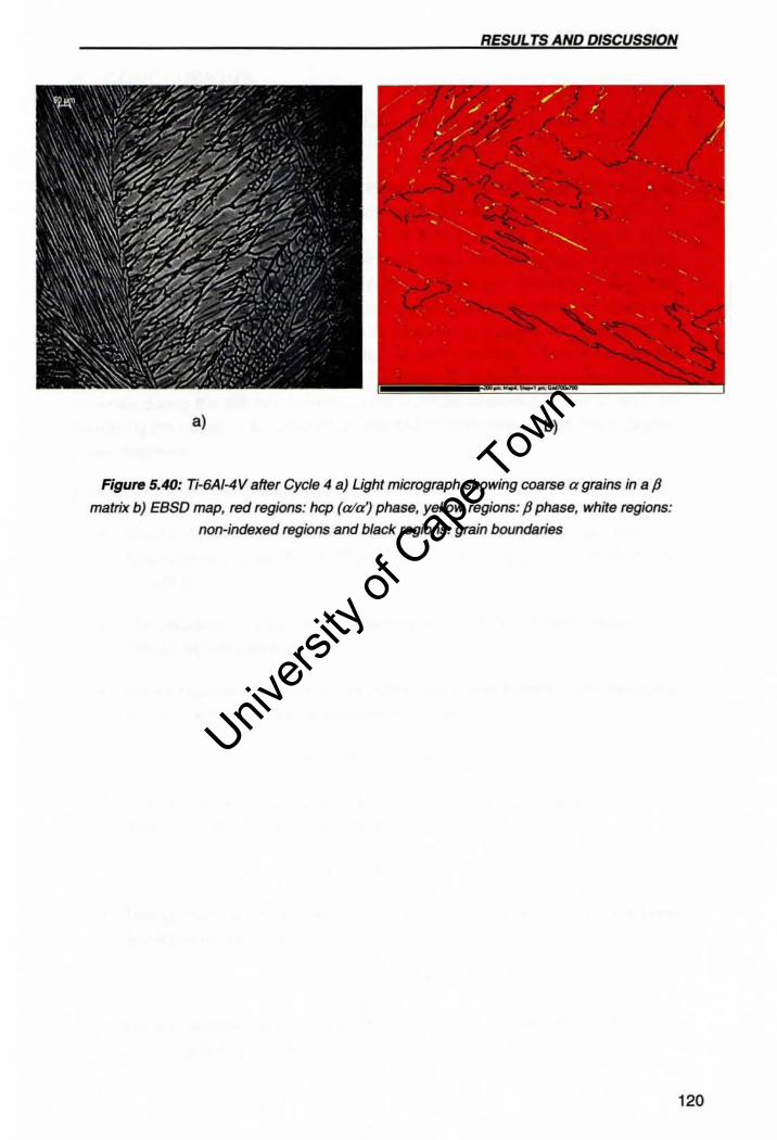
RESUL TS AND DISCUSSION
a) b)
Figure 5.40: Ti-6AJ-4 V after Cycle 4 a) Ught micrograph showing coarse a grains in 8 p matrix b) EBSD map, red regions: hcp (a/a') phase, yellow regions: P phase, white regions:
non-indexed regions and black regions: grain boundaries
120
Univers
ity of
Cap
e Tow
n
CONCLUSIONS
6 CONCLUSIONS
The push-rod dilatometer was successfully modified to act as a dual functioning
dilatometer/hydrogen furnace.
Dilatometry with in-situ hydrogenation thermal cycles was successfully used to
monitor the real-time phase transformation behaviour of both CP Ti and Ti-6AI-4V,
before, during and after hydrogenation. This technique was also used to show
marked differences and similarities in terms of phase transformations of these two
materials. Dilatometry was used to monitor the hydrogen absorption (uptake of
hydrogen) and desorption (expulsion of hydrogen) process by means of strain and
COTE curves. Furthermore, the addition of hydrogen to a stable CP Ti and the Ti-
6AI-4V alloy caused the phase composition of both materials to be altered coupled
with the formation of hydride phases. The level of hydrogen absorption in both
materials during the different thermal cycles could be estimated. This was done by
combining the output of the dilatometry and SEM/EBSD analysis with the published
phase diagrams.
A series of specific conclusions were drawn:
• Dilatometry was able to estimate the limit of hydrogen absorbed during the
hydrogenation cycle; in CP Ti this was ±40at%H and in Ti-6AI-4V it was
>15at%H
• The sequence of phase transformations for CP Ti during and hydrogenation
differed significantly from Ti-6AI-4V
• During hydrogenation (Cycle 1) in CP Ti, the phase transformation sequence
during heating could be summarised as follows:
• During hydrogenation (Cycle 1) in CP Ti, the phase transformation sequence
during cooling could be summarised as follows:
PH -+ aH + hydride
• During hydrogenation (Cycle 1) in Ti-6AI-4V the phase transformation
sequence during heating could be summarised as follows:
a + P -+ aH + PH -+ aH + PH + 8 -+ PH
• During hydrogenation (Cycle 1) in Ti-6AI-4V the phase transformation
sequence during cooling could be summarised as follows:
121
Univers
ity of
Cap
e Tow
n
CONCLUSIONS
• The uptake of hydrogen only occurred from ±550°C for both CP Ti and
Ti-6AI-4V
• Hydrogen caused the lattice expansion of CP Ti and Ti-6AI-4V during
hydrogenation (Cycle 1), which was seen by the strain and COTE curves
• Hydrogen in solid solution lowered the f3-transus of CP Ti to - 300°C as
predicted by the Ti-H phase diagram.
122
Univers
ity of
Cap
e Tow
n
FUTURE WORK
7 FUTURE WORK
The following recommendations are made in order to further understand the phase
transformation behaviour during each thermal cycle for both CP Ti and Ti-6AI-4V:
• Water quench experiments during each thermal cycle at pertinent
temperatures should be devised in order to monitor phase transformations at
critical temperatures
• Since this project only focussed on non-isothermal phase transformations,
TTT curves could not be constructed during each thermal cycle. Hence, a
series of isothermal treatments should be performed for each thermal cycle at
pertinent temperatures. This will allow for the further monitoring the kinetics of
phase transformations of CP Ti and Ti-6AI-4V before, during after
hydrogenation
• Since the amount of hydrogen could not be accurately quantified during the
hydrogen absorption and desorption process, the phase diagrams for Ti-H
and Ti-6AI-4V could not be accurately used to quantify the phases present
using the lever rule. Hence, a technique should be devised to accurately
quantify the amount of hydrogen present in the specimen
• Quantitative phase analysis should be performed on the EBSD maps in order
to understand how the addition of hydrogen altered the phase composition of
CP Ti and Ti-6AI-4V during and after hydrogenation. This would require more
extensive EBSD sampling of the microstructure
• Further quantitative phase and hydrogen content analysis should be
performed on Cycle 4 in order to understand the post-hydrogenation
behaviour of CP Ti and Ti-6AI-4V and to ascertain whether dehydrogenation
was successful in removing all the hydrogen from the specimen
123
Univers
ity of
Cap
e Tow
n
REFERENCES
8 REFERENCES
1. O.N. Senkov and F. H. Froes, Thermohydrogen processing of titanium alloys, International Journal of Hydrogen Energy 24 (1999), 565-576.
2. H. Wipf (Editor), Hydrogen in metals iii, Springer, 1997.
3. A. D. Mcquillian, An experimental and thermodynamic investigations of the hydrogen-titanium system, Proceedings of the Royal Society of London Series A 204 (1951), 309-322.
4. A. San-Martin and F. D. Manchester, The H-Ti (hydrogen-titanium) system, Journal of Phase Equilibria 8 (1987), 30-42.
5. B. A. Kolachev, Reversible alloying of titanium alloys with hydrogen, Metal Science and Heat treatment 35 (1993), 586-596.
6. J.I. Qazi, O. N. Senkov, J. Rahim and A. Genc, Phase transformations in Ti-6AI-4V-xH alloys, Metallurgical and Materials Transactions A 32A (2001), 2453-2463.
7. A. Guitar, G. Vigna and M. I. Luppo, Microstructure and tensile properties after thermohydrogen processing of Ti-6AI-4V, Journal of Mechanical behaviour of Biomedical Materials 2 (2009), 156-163.
8. K. L. Housley, Black sand: The history of titanium, Metal Management Aerospace, Inc., 2007.
9. E. Tal-Gautelmacher and D.Eliezer, The hydrogen embrittlement of titaniumbased alloys, JOM Journal of Minerals, Metals and Materials Society 57 (2005), no. 9, 46-49
10. S. Lathabai, B. L. Jarvis and K. J. Barton, Comparison of keyhole and conventional gas tungsten arc welds in commercially pure titanium, Materials Science and Engineering A299 (2001),81-93.
11. RR Pawar and V. T. Deshpande, The anisotropy of the thermal expansion of a-titanium, Acta Crystallography A24 (1968),316-317.
12. R Boyer, E. W. Collings and G. Welsch, Materials properties handbook: Titanium alloys, Materials Park (OH): ASM International, 1994.
13. C. Wu, V. Kumar, J. Liau, F. L'Esperance and G. Baker, "99.0ti," eFunda (Engineering Fundamentals) online, 2010.
14. W. F. Smith, "Structure and properties of engineering alloys," McGraw-Hili Publishing Co., 1981.
15. H. K. D. H. Bhadeshia, "Metallurgy of titanium and its alloys," University of Cambridge, Cambridge, 2004.
16. C. Leyens and M.Peters, Titanium and titanium alloys: Fundamentals and applications, Wiley-VCH Verlag GmbH & Co, 2003.
124
Univers
ity of
Cap
e Tow
n
REFERENCES
17. J. L. Murray (Editor), The AI-Ti (Aluminium-Titanium) phase system. Phase diagrams of binary titanium alloys, ASM, 1987.
18. D. R. Askerland, The science and engineering of materials, Stanely Thornes Ltd, 1998.
19. J.W. Elmer, T. A. Palmer and S. S. Babu, In situ observations of lattice expansion and transformation rates of a and fJ phases in Ti-6AI-4 V, Materials Science and Engineering A 391 (2005), 104-113.
20. C. Wu, V. Kumar, J. Liau, F. L'Esperance and G. Baker, "Ti-6AI-4V," eFunda (engineering fundamentals) online, 2010.
21. C. Garcia de Andries, F. G. Caballero, C. Capdevila and L. F. Alvarez, Application of dilatometric analysis to the study of solid-solid phase transformations in steels, Materials Characterization 48 (2002), 101-111.
22. M. Motyka and J. Sieniawski, The influence of initial plastic deformation on microstructure and hot plasticity of a+fJ titanium alloys, Archives of Materials Science and Engineering 41 (2010), 95-103.
23. N.S. Reddy, C. S. Lee, J.H. Kim and S. L. Semiatin, Determination of the beta-approach curve and the beta-transus temperature for the titanium alloys using sensitivity analysis of a trained neural network, Materials Science and Engineering A434 (2006),218-226.
24. M. Wei, A. J. Ruys and M. V. Swain, Interfacial bond strength of electrophoretically deposited hydroxyapatite coatings on metals, Journal of Materials Science: Materials in Medicine 10 (1999), 401-409.
25. S. Tamirisakandala, R. B. Bhat and D. B. Miracle, Effect of boron on the beta transus of Ti-6AI-4V alloy, Scripta Materialia 53 (2005), 217-222.
26. S. Malinov, Z.Guo, W. Sha and A. Wilson, Differential scanning calorimetry study and computer modelling of fJ to a phase transformation in a Ti-6AI-4 V alloy, Metallurgical and Materials Transactions 32A (2001), 879-887.
27. A. A. Ilyin, B. A. Kolachev and A. M. Mamanov, "Titanium '92: Science and technology," F. H. Froes and I. Caplan (Editors), vol. 1, TMS, Warrendale, PA, 1992, pp. 941-947.
28. W. R. Kerr, P. R. Smith, M. E. Rosenblum, F. J. Gurney, Y. R. Mahajan and L. R. Bidwell, "Titanium 80: Science and technology," H. Kimura and O. Izumi (Editors), vol. 4, TMS, Warrendale, PA, 1980, pp. 2477-2486.
29. R. Shivpuri, J. Hua, P. Mittal and A. K. Srivastava, "Industrial,welding and systems engineering," The Ohio State University, Columbus, USA, 2002, pp. 1-4.
30. S.L. Semiatin, S. L. Knisley, P. N. Fagin, F. Zhang and D. R. Barker, Microstructure evolution during alpha-beta heat treatment of Ti-6AI-4 V, Metallurgical and Materials Transactions A 34A (2003),2377-2386.
31. W. Sha and Z.Guo, Letter: Phase evolution of Ti-6AI-4V during continuous heating, Journal of Alloys and Compounds 290 (1999), L3-L7.
125
Univers
ity of
Cap
e Tow
n
REFERENCES
32. R. Filip, K. Kubiak, W. Ziaja and J. Sieniawski, The effect of the microstructure on the mechanical properties of the two-phase titanium alloys, Journal of Materials Processing Technology 133 (2003),84-89.
33. D. Phelan, M. Reid, N. Stanford and R. Dippenaar, In-situ observations of phase transformations in titanium, JOM Journal of Minerals, Metals and Materials Society 58 (2006), 67-69.
34. T. Ahmed and H. J. Jack, Phase transformation during cooling in a+/3 titanium alloys, Materials Science and Engineering A 243 (1998), 206-211.
35. M. R. Plichta, J. C. Williams and H. I. Aaronson, On the existence of /3 to am transformation in the alloy systems Ti-Ag, Ti-Au and Ti-Si, Metallurgical and Materials Transactions A 8 (1977), 1885-1892.
36. E. W. C. R. Boyer, and G. Welsch (Editor), Material properties handbook: Titanium alloys, ASM International, 1994.
37. X.L. Han, Q. Wang, D. L. Sun, T. Sun and Q. Guo, First principle study of hydrogen diffusion in alpha Ti, International Journal of Hydrogen Energy 34 (2009), 3983-3987.
38. C.P. Liang and H. R. Gong, Fundamental influence of hydrogen on the various properties of a-titanium, International Journal of Hydrogen Energy 35 (2010),3812-3816.
39. D. Eliezer, N. Eliaz, O. N. Senkov and F. H. Froes, Positive effects of hydrogen in metals, Materials Science and Engineering A 280 (2000), 220-224.
40. E. Tal-Gautelmacher, D. Eliezer and D. Eylon, The effects of low fugacity hydrogen in duplex and beta-annealed Ti-6AI-4V alloy, Materials Science and Engineering A 381 (2004), 230-236.
41. A. Lopez-Suarez, J. Rickards and R. Trejo-Luna, Analysis of hydrogen absorption by Ti and Ti-6AI-4V using the ERDA technique, International Journal of Hydrogen Energy 28 (2003), 1107-1113.
42. W. R. Kerr, The effect of hydrogen as a temporary alloying element on the microstructure and tensile properties of Ti-6AI-4V, Metallurgical and Materials Transactions A 16 (1981),1077-1087.
43. R. J. Smickley and L. E. Darid, US Patent no: 4505746 1985.
44. L. Levin, R. G. Vogt, D. Eylon and F. H. Froes, 5th International conference on Titanium. In, Deutsche Gesellshaft fur Metallkunde, 1984, p.App. 2107-2114.
45. C. F. Yolton and F. H. Froes, vol. US Patent no: 4219357, 1980.
46. 6th International conference on Titanium. In, Les Editions de Physique, 1988, p.App. 1641-1646.
126
Univers
ity of
Cap
e Tow
n
REFERENCES
47. N. Ninomi, B. Gong, T. Kobayashi, T. Ohyabu and O. Toriyama, Fracture characteristics of Ti-6AI-4V and Ti-5AI-2.5Fe with refined microstructure using hydrogen, Metallurgical and Materials Transactions A 26 (1995), 1141-1151.
48. A. A. lIyin, I. S. Polkin, A. M. Mamonov and V. K. Nosov, "Thermohydrogen treatment- the base of hydrogen technology of titanium alloys," Titanium '95: Science and Technology, vol. 4, 1995.
49. H. Okamoto, H-Ti (hydrogen-titanium), Journal of Phase Equilibria and Diffusion: Supplemental Literature Review: Section III (2011).
50. J.I. Qazi, O. N. Senkov, J. Rahim and F. H. S. Froes, Kinetics of martensite decomposition in Ti-6AI-4V-xH, Materials Science and Engineering A 359 (2003), 137-149.
51. Z. Sun, H. Hou, W. Zhou, Y. Wang and Z. Li, The effect of hydrogen on microstructures evolution and deformation behaviour of Ti-6AI-4V alloys, Journals of Alloys and Compounds 476 (2009), 550-555.
52. J. Zhao, H. Ding, W. Zhao, X. Tian, H. Hou and Y. Wang, Influence of hydrogenation on microstructures and microhardness of Ti-6AI-4V alloy, Transactions Nonferrous Metals Society of China 18 (2008), 506-511.
53. D.B. Shan, Y. Y. Zong, T. F. Lu and Y. Lv, Microstructural evolution and formation mechanism of fcc titanium hydride in Ti-6AI-4V-xH alloys, Journal of Alloys and Compounds 427 (2007), no. 229-234.
54. G. Domizzi, M. I. Luppo and G. Vigna, Microstructural features of the hydrogenation process in Ti grade 2, Journal of Alloys and Compounds 424 (2006),193-198.
55. C.C. Shen and T. P. Perng, Pressure-composition isotherms and reversible hydrogen-induced phase transformations in Ti-6AI-4V, Acta Materialia 55 (2007),1053-1058.
56. D. Setoyama, J. Matsunaga, H. Muta, M. Uno and S. Yamanaka, Mechanical properties of titanium hydride, Journal of Alloys and Compounds 381 (2004), 215-220.
57. L. Luo, Y. Su, J. Guo and H. Fu, Formation of titanium hydride in Ti-6AI-4V alloy, Journal of Alloys and Compounds 45 (2006), no. 140-144.
58. H. K. D. H. Bhadeshia, Bainite: Overall transformation kinetics, Journal de Physique Archives 43 (1982), no. C4, 433-448.
59. F. J. Humpreys, Review grain and sub grain characterization by electron back scatter diffraction, Journal of Materials Science 36 (2001), 3833-3854.
60. "Basics of EBSD," vol. 2010, Oxford instruments PLC, Oxfordshire, 2005.
61. O. N. Senkov, B. C. Chakoumakos, J. J. Jonas and F. H. Froes, Effect of temperature and hydrogen concentration on the lattice parameter of the beta titanium, Materials Research Bulletin 36 (2001),1431-1440.
127
Univers
ity of
Cap
e Tow
n
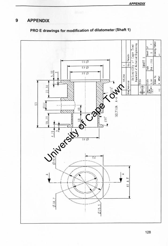
APPENDIX
9 APPENDIX
PRO E drawings for modification of dilatometer (Shaft 1)
,,,, C7'VJ
-I~ '1
n ~ 1'F0 ~ . , ~ ,
~~' ., n I ~ I
I I-• I
C· -~ . . - -- j- - ----!-~ I , I
- i - '-~ ~ ~ I 0
'" - I -~"' --t
- .,
I. I
.1 ~
~ -
~ ---~ ~- ;S0 1_ ! '. ,
, •
I I i l , , , • , ' . , ') i- -:------1
< . <
o 0-w w ~
-- -. --u : I- ,; . -~ ~.::;
-= .... "::-; . --... -. ":;: I-I-::j u ,
- 5: ~~ -:; .... --.. :: - >
_J ~ <
~
-.. - : ~ .... :
v. _ .... . ~ .:
i' ;,;-• -0 ,'" ;:; .:~-
128
Univers
ity of
Cap
e Tow
n
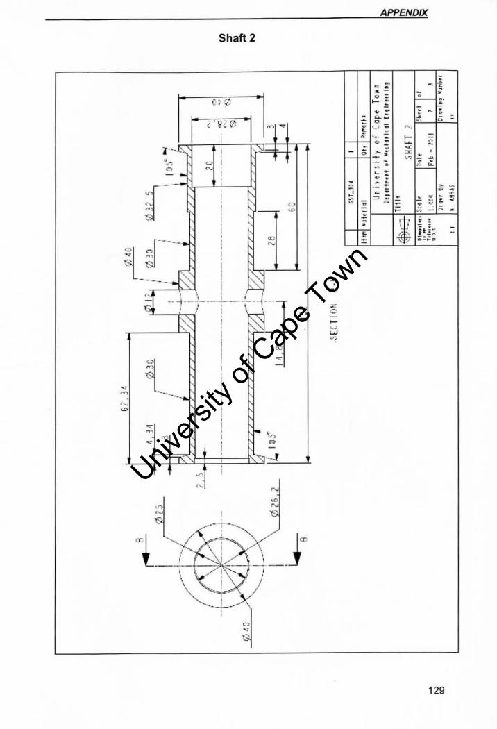
Shaft 2
r IB/ (!; "I ~_=-~l\.;t-t~!,! ---t~!:hn
~ O __ :~_"l.' _: ! _~'I __
I
~
I -
I
I i , I , :]. ~ .... I , 0
I , ~"" -~ , ~
i
"
o ,p
~' -
~ , "' z <> -~ u w ~
-.. -" -- ..
APPENDIX
& : ' . -o ~ ..
=
,- . -.
- ~ ~~. :: .... ~ :to <i :
,', , ~., .:. ... ~
--., -; , -
129
Univers
ity of
Cap
e Tow
n
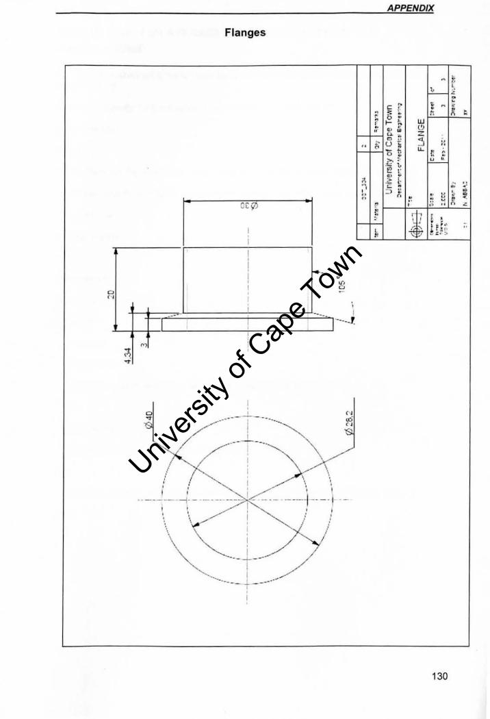
0
"
., ~ ,~
'"
Flanges
I I , , ! I ~ -, I
, [
--- , I
---,
--[ , , ,
.. ! , j i i ____ --i I ',_ i~/- -------:
, ' ____ I I --------[ '\ '
\ ~ : \ '" -- ' ~ -t --
.......... I - T - - ---'
, I , , ..
\ I
----'
. . " ~ , "
APPENDIX
, ,
~ ~ f
... ~;
" , <
- " - .-. . ... . _ II>
,: ::: ~ ,. ,~ "n .!.
130
Univers
ity of
Cap
e Tow
n
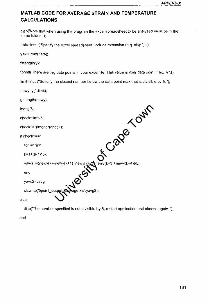
APPENDIX
MATLAB CODE FOR AVERAGE STRAIN AND TEMPERATURE
CALCULATIONS
disp('Note that when using the program the excel spreadsheet to be analysed must be in the same folder. ');
data=input('Specify the excel spreadsheet, include extension (e.g .xls): ','s');
y=xlsread( data);
f=length(y);
fprintf(There are %g data points in your excel file. This value is your data point max. \n',f);
limit=input('Specify the closest number below the data point max that is divisible by 5: ');
newy=y(1 :Iimit);
g=length(newy);
inc=g/5;
check=limiU5;
check2=isinteger( check);
if check2==1
for i=1 :inc
k=1 +( (i-1 )*5);
yavg( i)=(newy(k )+newy( k+1 )+newy(k+2)+newy(k+3)+newy(k+4) )/5;
end
yavg2=yavg.';
xlswrite('5point_ output_average .xls', yavg2);
else
disp('The number specified is not divisible by 5, restart application and choose again. ');
end
131
Univers
ity of
Cap
e Tow
n
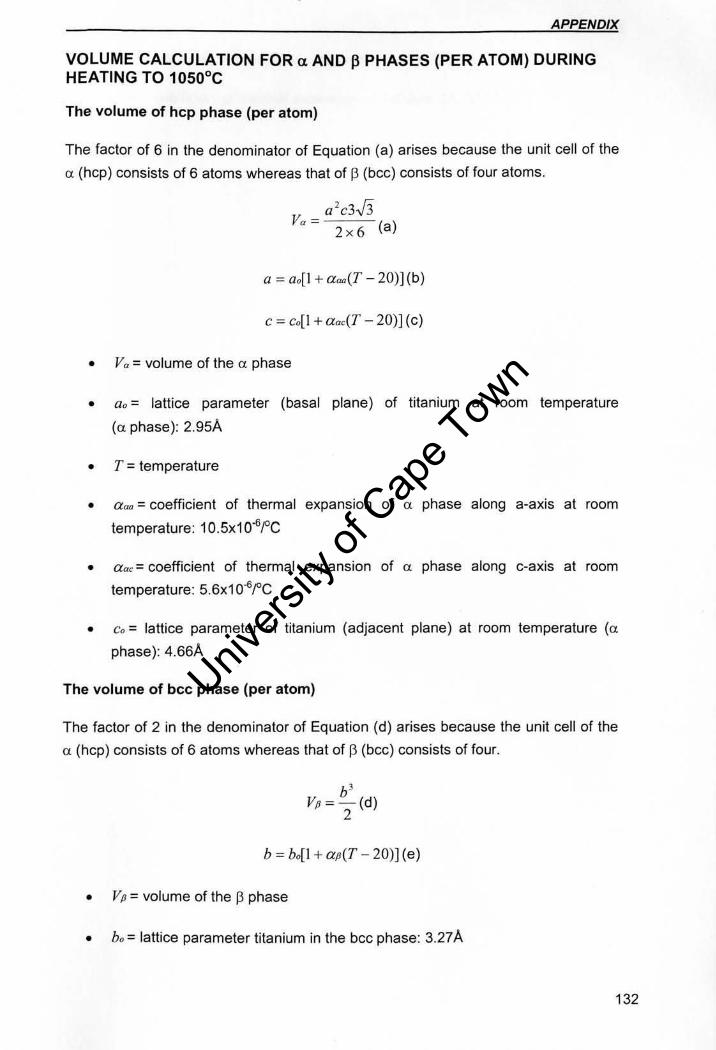
APPENDIX
VOLUME CALCULATION FOR a AND ~ PHASES (PER ATOM) DURING HEATING TO 10S0°C
The volume of hep phase (per atom)
The factor of 6 in the denominator of Equation (a) arises because the unit cell of the
a (hcp) consists of 6 atoms whereas that of P (bcc) consists of four atoms.
Va a'c3.f3
2 X 6 (a)
a = a, [1 + a =(T - 20)] (b)
c = c,[1 + a ao(T - 20)] (e)
• Va = volume of the a phase
• a o = lattice parameter (basal plane) of titanium at room temperature
(et phase): 2.9SA
• T = temperature
• aoo = coefficient of thermal expansion of a phase along a-axis at room
temperature: 10.Sx10~fC
• aac = coefficient of thermal expansion of a phase along c-axis at room
temperature: 5.6x10⁻⁶rC
• Cd = lattice parameter of titanium (adjacent plane) at room temperature (a
phase): 4.66A
The volume of bee phase (per atom)
The factor of 2 in the denominator of Equation (d) arises because the unit cell of the
a (hcp) consists of 6 atoms whereas that of [3 (bcc) consists of four.
b' Vp = - (d)
2
b = b,,[1 + a p(T - 20)] (e)
• Vp = volume of the p phase
• bo = lattice parameter titanium in the bcc phase: 3.27 A
132
Univers
ity of
Cap
e Tow
n
APPENDIX
• T = temperature (increasing at increments of 1 a°C)
• afJ = coefficient of thermal expansion of f3 phase: 14.1 x1 a-61°C
133
Univers
ity of
Cap
e Tow
n


