arX

iv:a

stro

-ph/

9710

131v

1 1

3 O

ct 1

997

06(03.13.2; 03.13.6; 03.13.5; 06.15.1) ASTROPHYSICS

The art of fitting p-mode spectra: Part II. Leakage andnoise covariance matrices

Thierry Appourchaux1, Maria-Cristina Rabello-Soares1, Laurent Gizon1,2

1 Space Science Department of ESA, ESTEC, NL-2200 AG Noordwijk2 W.W.Hansen Experimental Physics Laboratory, Center for Space Science and Astrophysics, Stanford University, Stanford,

CA 94305-4085, USA

Received / Accepted

Abstract. In Part I we have developed a theory for fittingp-mode Fourier spectra assuming that these spectra have amulti-normal distribution. We showed, using Monte-Carlosimulations, how one can obtain p-mode parameters using’Maximum Likelihood Estimators’. In this article, here-after Part II, we show how to use the theory developed inPart I for fitting real data. We introduce 4 new diagnos-tics in helioseismology: the (m, ν) echelle diagramme, thecross echelle diagramme, the inter echelle diagramme, andthe ratio cross spectrum. These diagnostics are extremelypowerful to visualize and understand the covariance ma-trices of the Fourier spectra, and also to find bugs in thedata analysis code. These diagrammes can also be used toderive quantitative information on the mode leakage andnoise covariance matrices. Numerous examples using theLOI/SOHO and GONG data are given.

Key words: Methods: data analysis – statistical – obser-vational – Sun: oscillations

1. Introduction

The physics of the solar interior is known from inversionof solar p-mode frequencies and splittings. These measure-ments are derived from fitting p-mode Fourier spectra.Schou (1992) was the first one to assume a multi-normaldistribution for p-mode Fourier spectra and using a realleakage matrix. Following this pioneering work, Appour-chaux et al. (1997) (hereafter Part I), generalized the the-oretical background for fitting p-mode Fourier spectra tocomplex leakage matrix, and included explicitly the cor-relation of the noise between the Fourier spectra. UsingMonte-Carlo simulations, we showed that our fitted pa-rameters were unbiased. We also studied systematic errorsdue to an imperfect knowledge of the leakage covariancematrix. Unfortunately, a theoretical knowledge of fitting

Send offprint requests to: thierrya@so.estec.esa.nl

data is not enough as only real data will teach us if our ap-proach is correct. Contrary to fitting p-mode power spec-tra, the process of fitting the Fourier spectra as describedin Part I is rather difficult to understand and visualize.Schou (1992) gave a few diagnostics for understandinghow the Fourier spectra are fitted but without showingan easy way to visualize the covariance matrices.

In this paper, we show how one can easily visualizethe mode and noise correlation matrices, and then derivethe mode leakage matrix. In the first section, we describe4 new diagrammes that have various diagnostics power.In the second section, we describe how we use those di-agrammes for inferring the leakage and noise covariancematrices for the data of the Luminosity Oscillations Im-ager (LOI) on board the Solar and Heliospheric Observa-tory (SOHO) data (Appourchaux et al, 1997), and for thedata of the Global Oscillations Network Group (GONG)(Hill et al, 1996). The LOI time series starts on 27 March1996 and ends on 27 March 1997 with a duty cycle greaterthan 99%. The GONG time series starts on 27 August1995 and ends on 22 August 1996 with a 75% duty cy-cle. In the last section we conclude by emphasizing theusefulness of these diagrammes.

2. Diagnostics for helioseismic data analysis

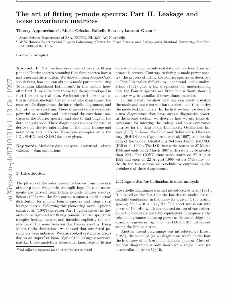
The echelle diagramme was first introduced by Grec (1981).It is based on the fact that the low-degree modes are es-sentially equidistant in frequency for a given l; the typicalspacing for l = 0 is 136 µHz. The spectrum is cut intopieces of 136 µHz which are stacked on top of each other.Since the modes are not truly equidistant in frequency, theechelle diagramme shows up power as distorted ridges; anexample is given in Fig. 1 for the LOI/SOHO instrumentseeing the Sun as a star.

Another useful diagramme was introduced by Brown(1985), the so-called (m, ν) diagramme which shows howthe frequency of an l, m mode depends upon m. Most of-ten this diagramme is only shown for a single n and forintermediate degrees l ≥ 10.

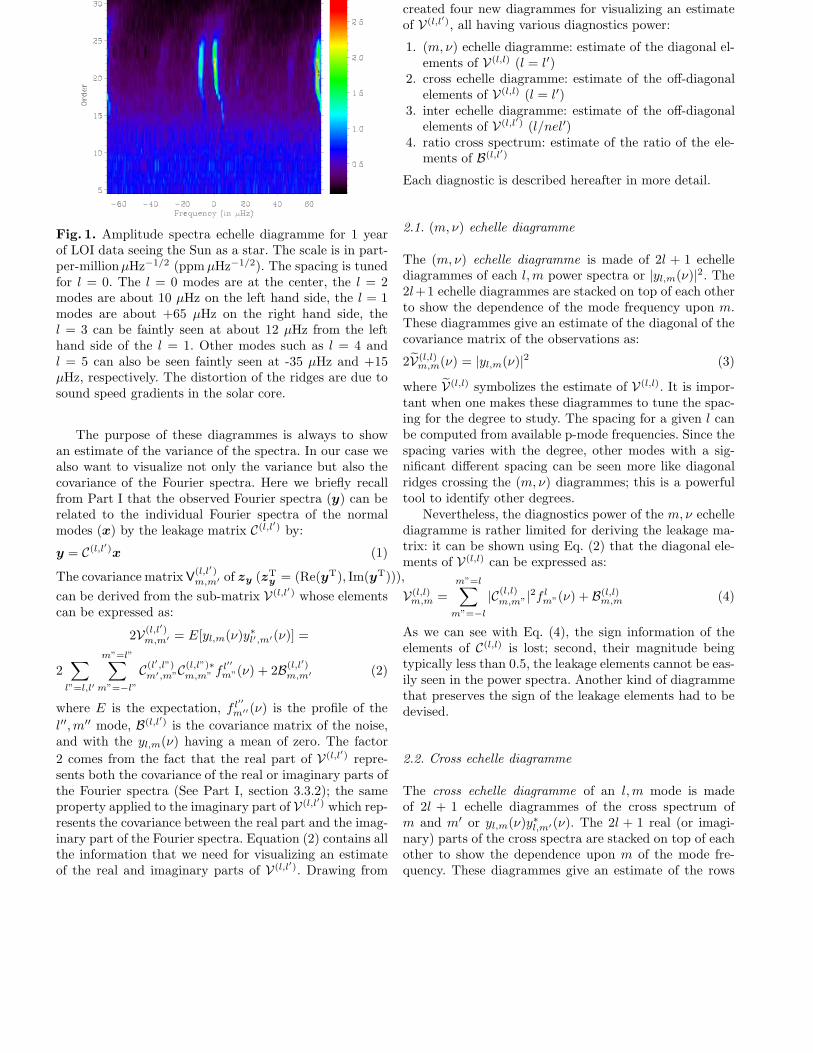
Fig. 1. Amplitude spectra echelle diagramme for 1 yearof LOI data seeing the Sun as a star. The scale is in part-per-millionµHz−1/2 (ppm µHz−1/2). The spacing is tunedfor l = 0. The l = 0 modes are at the center, the l = 2modes are about 10 µHz on the left hand side, the l = 1modes are about +65 µHz on the right hand side, thel = 3 can be faintly seen at about 12 µHz from the lefthand side of the l = 1. Other modes such as l = 4 andl = 5 can also be seen faintly seen at -35 µHz and +15µHz, respectively. The distortion of the ridges are due tosound speed gradients in the solar core.

The purpose of these diagrammes is always to showan estimate of the variance of the spectra. In our case wealso want to visualize not only the variance but also thecovariance of the Fourier spectra. Here we briefly recallfrom Part I that the observed Fourier spectra (y) can berelated to the individual Fourier spectra of the normalmodes (x) by the leakage matrix C(l,l′) by:

y = C(l,l′)x (1)

The covariance matrix V(l,l′)m,m′ of zy (zT

y= (Re(yT), Im(yT))),

can be derived from the sub-matrix V(l,l′) whose elementscan be expressed as:

2V(l,l′)m,m′ = E[yl,m(ν)y∗

l′,m′(ν)] =

2∑

l”=l,l′

m”=l”∑

m”=−l”

C(l′,l”)m′,m”C

(l,l”)∗m,m” f l′′

m”(ν) + 2B(l,l′)m,m′ (2)

where E is the expectation, f l′′

m′′(ν) is the profile of the

l′′, m′′ mode, B(l,l′) is the covariance matrix of the noise,and with the yl,m(ν) having a mean of zero. The factor

2 comes from the fact that the real part of V(l,l′) repre-sents both the covariance of the real or imaginary parts ofthe Fourier spectra (See Part I, section 3.3.2); the sameproperty applied to the imaginary part of V(l,l′) which rep-resents the covariance between the real part and the imag-inary part of the Fourier spectra. Equation (2) contains allthe information that we need for visualizing an estimateof the real and imaginary parts of V(l,l′). Drawing from

the usefulness of the diagrammes of Grec and Brown, wecreated four new diagrammes for visualizing an estimateof V(l,l′), all having various diagnostics power:

1. (m, ν) echelle diagramme: estimate of the diagonal el-ements of V(l,l) (l = l′)

2. cross echelle diagramme: estimate of the off-diagonalelements of V(l,l) (l = l′)

3. inter echelle diagramme: estimate of the off-diagonalelements of V(l,l′) (l/nel′)

4. ratio cross spectrum: estimate of the ratio of the ele-ments of B(l,l′)

Each diagnostic is described hereafter in more detail.

2.1. (m, ν) echelle diagramme

The (m, ν) echelle diagramme is made of 2l + 1 echellediagrammes of each l, m power spectra or |yl,m(ν)|2. The2l+1 echelle diagrammes are stacked on top of each otherto show the dependence of the mode frequency upon m.These diagrammes give an estimate of the diagonal of thecovariance matrix of the observations as:

2V(l,l)m,m(ν) = |yl,m(ν)|2 (3)

where V(l,l) symbolizes the estimate of V(l,l). It is impor-tant when one makes these diagrammes to tune the spac-ing for the degree to study. The spacing for a given l canbe computed from available p-mode frequencies. Since thespacing varies with the degree, other modes with a sig-nificant different spacing can be seen more like diagonalridges crossing the (m, ν) diagrammes; this is a powerfultool to identify other degrees.

Nevertheless, the diagnostics power of the m, ν echellediagramme is rather limited for deriving the leakage ma-trix: it can be shown using Eq. (2) that the diagonal ele-ments of V(l,l) can be expressed as:

V(l,l)m,m =

m”=l∑

m”=−l

|C(l,l)m,m”|

2f lm”(ν) + B(l,l)

m,m (4)

As we can see with Eq. (4), the sign information of theelements of C(l,l) is lost; second, their magnitude beingtypically less than 0.5, the leakage elements cannot be eas-ily seen in the power spectra. Another kind of diagrammethat preserves the sign of the leakage elements had to bedevised.

2.2. Cross echelle diagramme

The cross echelle diagramme of an l, m mode is madeof 2l + 1 echelle diagrammes of the cross spectrum ofm and m′ or yl,m(ν)y∗

l,m′(ν). The 2l + 1 real (or imagi-nary) parts of the cross spectra are stacked on top of eachother to show the dependence upon m of the mode fre-quency. These diagrammes give an estimate of the rows

(or columns) of the covariance matrix of the observationsas:

2V(l,l)m,m′(ν) = yl,m(ν)y∗

l,m′(ν) (5)

Of course when m = m′ we get the echelle diagrammes ofthe previous section. Only l + 1 cross echelle diagrammesare shown as the matrix V(l,l′) is hermitian by definition.

The imaginary part of the cross spectra has some di-agnostic power: it represents the correlation between thereal and imaginary parts of the Fourier spectra. When theleakage matrix is real, which is generally the case, thereis no correlation between the real and imaginary parts.Nevertheless the imaginary part could be helpful to finderrors in the filters applied to the images (See Part I, sec-tion 3.3.1).

It can be shown that the elements of V(l,l) can be ex-pressed as:

V(l,l)m,m′ = C

(l,l)m,m′f

lm′(ν) + C

(l,l)∗m′,mf l

m(ν) +∑

m”6=m′,m

C(l,l)m′,m”C

(l,l)∗m,m”f

l′′

m′′(ν) + B(l,l)m,m′ (6)

As we can see with Eq. (6), these diagrammes preserve thesign of the leakage matrix elements. In general, the cross

spectra for m, m′, representing V(l,l)m,m′ carries information

over the sign of the leakage elements C(l,l)m,m′ and C

(l,l)∗m′,m.

The other additional terms expressed as product of leakageelements are sometimes more difficult to interpret.

But the power of these diagrammes is not only re-stricted to checking the sign of the elements of the leak-age matrix. They are also real tools to get a first orderestimate of the leakage matrix. We have shown in Part I,that there is no difference between fitting data for whichthe leakage matrix is the identity, and data for which theleakage matrix is not. We showed in part I, that the co-variance matrix of x (x = C−1

y) can be written, similarlyto that of Eq. (2)), by the sum of 2 matrices: the first onerepresents the mode covariance matrix and is diagonal,and the second term represents the covariance matrix ofthe noise. Therefore, applying the inverse of the leakagematrix to the data should, in principle, remove all artificialmode correlations between the Fourier spectra of x: thiscan be verified using the cross echelle diagrammes. This isthe most powerful test for deriving the leakage matrices.

The cross echelle diagrammes are useful to verify thecorrelation within a given degree, but other degrees areknown to leak into the target degree, such as l = 6, 7 and8 into l = 1, 4 and 8, respectively. The purpose of the nextdiagramme is to assess the magnitude of these leakages.

2.3. Inter echelle diagramme

The inter echelle diagramme of an l, m mode for the de-gree l′ is made of 2l′ + 1 echelle diagrammes of the crossspectrum of l, m and l′, m′ or yl,m(ν)y∗

l′,m′(ν). The 2l′ + 1real part of the cross spectra are stacked on top of each

other to show the dependence upon m′. These diagrammesgive an estimate of the rows (or columns) of the covariancematrix of the observations as:

2Vm,m′(ν) = yl,m(ν)y∗l′,m′(ν) (7)

Similarly as for the cross echelle diagramme, it will help tovisualize the covariance matrix between different degrees,and to derive leakage elements of the full leakage matrixC(l,l′). One can derive an equation similar to Eq. (6) fordifferent degrees showing that the inter echelle diagrammecarries information over the sign of the leakage elements

C(l,l′)m,m′ and C

(l′,l)∗m′,m .

As mentioned above applying the inverse of the leakagematrix will help to verify to the first order that there is noartificial correlation due to the p modes. When differentdegrees are involved the full leakage matrix C(l,l′) has to beused, producing diagrammes that should have no artificialcorrelation due to the p modes.

2.4. Ratio cross spectrum

All the previous diagrammes are helpful to understandand visualize the mode covariance matrices. Unfortunately,due to the high signal-to-noise ratio, these diagrammescannot be used to evaluate the correlation of the noise inthe Fourier spectra. In between the p modes, these corre-lations can be more easily visualized as we have:

V(l,l)m,m′ ≈ B

(l,l)m,m′ (8)

But instead of visualizing B(l,l′), we prefer to look directlyat the correlation by computing the ratio of the cross spec-tra as:

˜B

(l,l′)m,m′

B(l,l)m,m

=(yl,m(ν)y∗

l,m′(ν)

|yl,m(ν)|2(9)

This ratio is called the ratio cross spectrum. The ratiocross spectrum gives an estimate of the ratio matrix R(l,l′)

(See Part I) which gives a better understanding of howmuch the noise background is correlated between the Fou-rier spectra. Nevertheless, in the p-mode frequency range,the ratio cross spectrum is more difficult to interpret asthe noise correlation is affected by the presence of themodes. By looking away from the modes (at high or lowfrequency) or by looking between the modes, one couldobtain a reasonable good estimate of the noise correlation.

3. Application to data

3.1. (m, ν) echelle diagramme for the LOI/SOHO data

Example of these diagrammes can be seen in Figs. 2, 3 and4 for 1 year of LOI data for l = 1, 2 and 5, respectively.It is important when one makes such diagrammes to tune

Fig. 2. (m, ν) echelle diagramme for 1 year of LOI data for l = 1. The scale is in ppmµHz−1/2. The spacing is tunedfor l = 1. (Left) The full diagramme centered on l = 1. The l = 3 modes are located about 15 µHz at the left handside of the l = 1. The l = 2 modes are on the right edge, while the l = 0 are on the opposite side. The l = 4 modes canbe seen around +40 µHz. (Right) The same diagramme but enlarged around l = 1. The frequency shift or splitting ofthe modes due to the solar rotation can be seen: the 2 patches of power for m = −1 and m = +1 are slightly displacedfrom each other. The artificial correlation between m = −1 and m = +1 is not as clear.

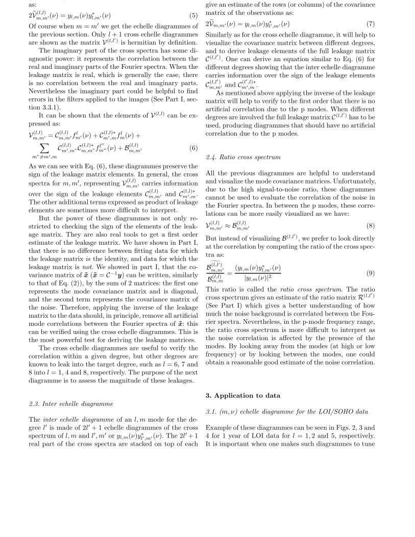
Fig. 3. (m, ν) echelle diagramme for 1 year of LOI data for l = 2. The scale is in ppmµHz−1/2. The spacing is tunedfor l = 2. (Left) The full diagramme centered on l = 2 with a spacing of 135. µHz. The l = 0 modes are located about10 µHz at the right hand side of the l = 2 modes. The l = 3 modes are on the right edge, while the l = 1 modes are onthe opposite side. The l = 4 modes are easily seen at about -25 µHz; the l = 5 starts to appear at +25 µHz. (Right)The same diagramme but enlarged around l = 2 with the l = 0 modes at the right hand side. The splitting of themodes is clear. Note the absence of the l = 0 modes for m = ±1

the spacing for the degree to study. For example, one cansee in Fig. 2 that the ridges of power of l = 0, 1, 2 and 3have different shapes than in Fig. 3. Other modes with asignificant different spacing can be seen more like diagonalridges crossing the (m, ν) diagrammes; this is a powerfultool to identify other degrees. In Fig. 4, the l = 5 (m, ν)echelle diagramme is clearly contaminated by an otherdegree, i.e. l = 8, which appears at different frequenciesdepending on m. For l = 5, m = −5, the l = 8, m = +8 isquite strong; while for l = 5, m = +5, this is l = 8, m = −8which shows up. This kind of ‘anti’-splitting behaviour is

typical of any aliasing degrees. It is more prominent in theLOI data because of the undersampling effect due to thelarge size of the LOI pixels.

3.2. A useful detail

Before using the other diagrammes on real data, we needto point out a very important property coming from theway the m signals are built. If the weights Wl,m applied

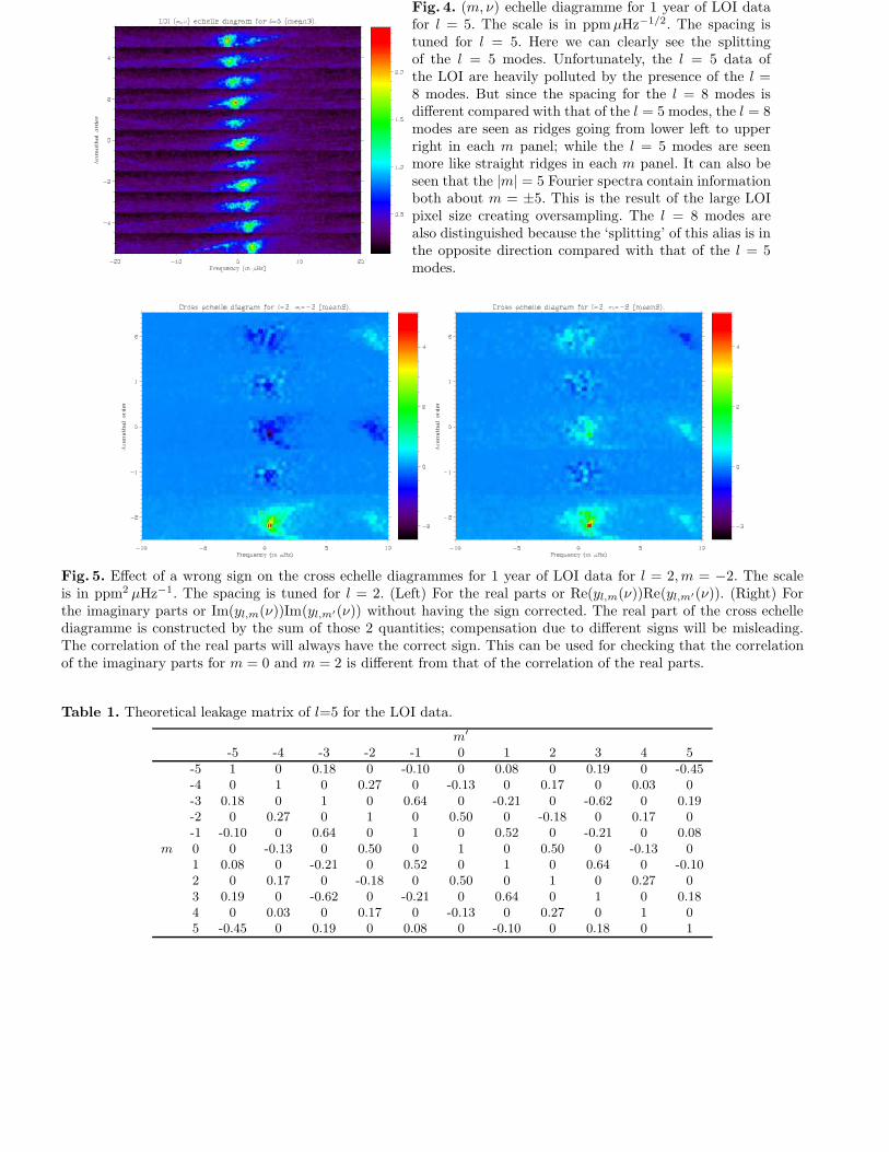
Fig. 4. (m, ν) echelle diagramme for 1 year of LOI datafor l = 5. The scale is in ppmµHz−1/2. The spacing istuned for l = 5. Here we can clearly see the splittingof the l = 5 modes. Unfortunately, the l = 5 data ofthe LOI are heavily polluted by the presence of the l =8 modes. But since the spacing for the l = 8 modes isdifferent compared with that of the l = 5 modes, the l = 8modes are seen as ridges going from lower left to upperright in each m panel; while the l = 5 modes are seenmore like straight ridges in each m panel. It can also beseen that the |m| = 5 Fourier spectra contain informationboth about m = ±5. This is the result of the large LOIpixel size creating oversampling. The l = 8 modes arealso distinguished because the ‘splitting’ of this alias is inthe opposite direction compared with that of the l = 5modes.

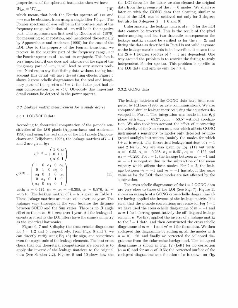
Fig. 5. Effect of a wrong sign on the cross echelle diagrammes for 1 year of LOI data for l = 2, m = −2. The scaleis in ppm2 µHz−1. The spacing is tuned for l = 2. (Left) For the real parts or Re(yl,m(ν))Re(yl,m′(ν)). (Right) Forthe imaginary parts or Im(yl,m(ν))Im(yl,m′(ν)) without having the sign corrected. The real part of the cross echellediagramme is constructed by the sum of those 2 quantities; compensation due to different signs will be misleading.The correlation of the real parts will always have the correct sign. This can be used for checking that the correlationof the imaginary parts for m = 0 and m = 2 is different from that of the correlation of the real parts.

Table 1. Theoretical leakage matrix of l=5 for the LOI data.

m′

-5 -4 -3 -2 -1 0 1 2 3 4 5

-5 1 0 0.18 0 -0.10 0 0.08 0 0.19 0 -0.45-4 0 1 0 0.27 0 -0.13 0 0.17 0 0.03 0-3 0.18 0 1 0 0.64 0 -0.21 0 -0.62 0 0.19-2 0 0.27 0 1 0 0.50 0 -0.18 0 0.17 0-1 -0.10 0 0.64 0 1 0 0.52 0 -0.21 0 0.08

m 0 0 -0.13 0 0.50 0 1 0 0.50 0 -0.13 01 0.08 0 -0.21 0 0.52 0 1 0 0.64 0 -0.102 0 0.17 0 -0.18 0 0.50 0 1 0 0.27 03 0.19 0 -0.62 0 -0.21 0 0.64 0 1 0 0.184 0 0.03 0 0.17 0 -0.13 0 0.27 0 1 05 -0.45 0 0.19 0 0.08 0 -0.10 0 0.18 0 1

to the images, to extract an l, m mode, have the sameproperties as of the spherical harmonics then we have:

Wl,m = W ∗l,−m (10)

which means that both the Fourier spectra of +m and−m can be obtained from using a single filter Wl,+m. TheFourier spectrum of +m will be in the positive part of thefrequency range, while that of −m will be in the negativepart. This approach was first used by Rhodes et al. (1979)for measuring solar rotation, and mentioned theoreticallyby Appourchaux and Andersen (1990) for the case of theLOI. Due to the property of the Fourier transform, werecover, in the negative part of the frequency range, notthe Fourier spectrum of −m but its conjugate. This fact isvery important, if one does not take care of the sign of theimaginary part of −m, it will lead to very serious prob-lem. Needless to say that fitting data without taking intoaccount this detail will have devastating effects. Figure 5shows 2 cross echelle diagrammes for the real and imagi-nary parts of the spectra of l = 2; the latter part had nosign compensation for m < 0. Obviously this importantdetail cannot be detected in the power spectra.

3.3. Leakage matrix measurement for a single degree

3.3.1. LOI/SOHO data

According to theoretical computation of the p-mode sen-sitivities of the LOI pixels (Appourchaux and Andersen,1990) and using the real shape of the LOI pixels (Appour-chaux and Telljohann, 1996), the leakage matrices of l = 1and 2 are given by:

C(1,1) =

1 0 α0 1 0α 0 1

C(2,2) =

1 0 α1 0 α4

0 1 0 α2 0α3 0 1 0 α3

0 α2 0 1 0α4 0 α1 0 1

(11)

with: α = 0.474, α1 = α3 = −0.308, α2 = 0.576, α4 =−0.216. The leakage matrix of l = 5 is given in Table 1.These leakage matrices are mean value over one year. Theleakages vary throughout the year because the distancebetween SOHO and the Sun varies. There is no B angleeffect as the mean B is zero over 1 year. All the leakage el-ements are real as the LOI filters have the same symmetryas the spherical harmonics.

Figure 6, 7 and 8 display the cross echelle diagrammefor l = 1, 2 and 5, respectively. From Figs. 6 and 7, wecan directly verify using Eq. (6) the sign, and sometimeseven the magnitude of the leakage elements. The best crosscheck that our theoretical computations are correct is toapply the inverse of the leakage matrices to the originaldata (See Section 2.2). Figures 9 and 10 show how the

artificial correlations (or m leaks) can be removed fromthe LOI data; for the latter we also cleaned the originaldata from the presence of the l = 0 modes. We shall seelater on with the GONG data that cleaning, similar tothat of the LOI, can be achieved not only for 2 degreesbut also for 3 degrees (l = 1, 6 and 9).

Unfortunately, the leakage matrix of l = 5 for the LOIdata cannot be inverted. This is the result of the pixelundersampling and has two dramatic consequences: theleakage matrix cannot be verified as for the l = 2, andfitting the data as described in Part I is not valid anymoreas the leakage matrix needs to be invertible. It means thatthe 2l + 1 Fourier spectra of l = 5 are dependent. Oneway around the problem is to restrict the fitting to trulyindependent Fourier spectra. This problem is specific tothe LOI data and applies only for l ≥ 4.

3.3.2. GONG data

The leakage matrices of the GONG data have been com-puted by R.Howe (1996, private communication). We alsocomputed similar leakage matrices using the equations de-veloped in Part I. The integration was made in the θ, φplane with θmax = 65.2◦, φmax = 53.5◦ without apodiza-tion. We also took into account the effect of subtractingthe velocity of the Sun seen as a star which affects GONGinstrument’s sensitivity to modes only detected by inte-grated sunlight instrument (mainly the modes for whichl + m is even). The theoretical leakage matrices of l = 1and 2 for GONG are also given by Eq. (11) but with:α = −0.55, α1 = −0.268, α2 = 0.451, α3 = −0.122, andα4 = −0.290. For l = 1, the leakage between m = −1 andm = +1 is negative due to the subtraction of the meanvelocity which affects these modes. For l = 2, the leak-age between m = −1 and m = +1 has about the samevalue as for the LOI; these modes are not affected by thesubtraction.

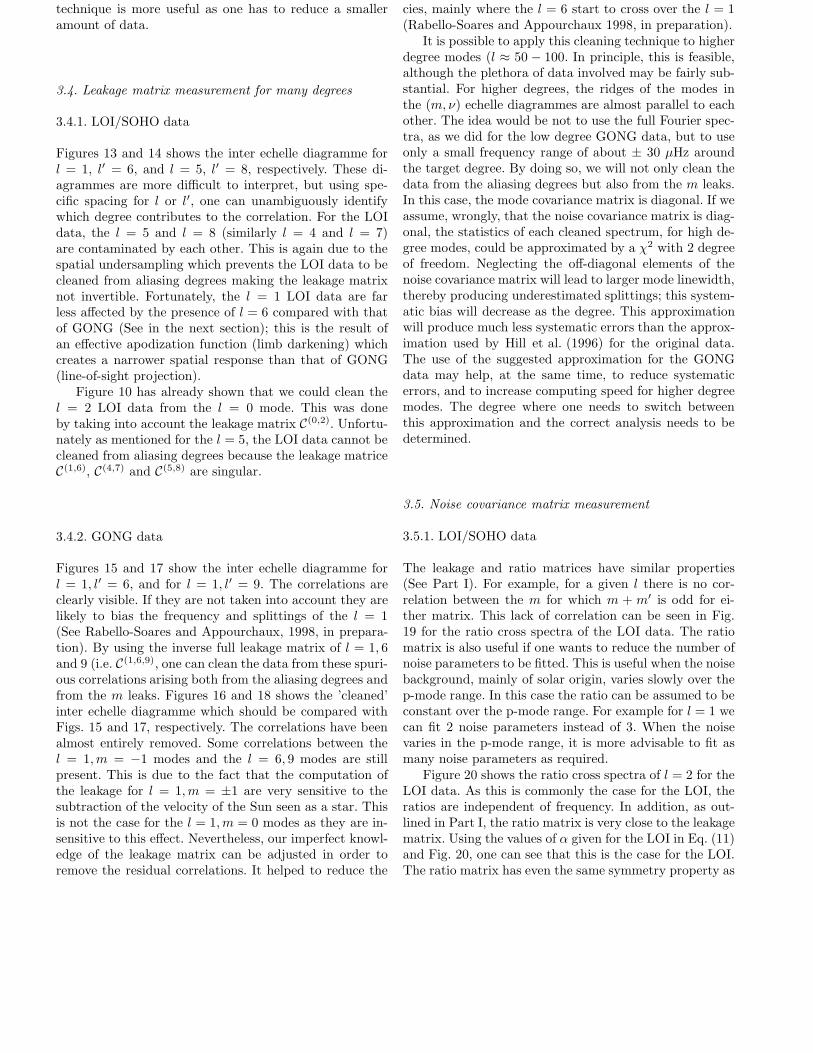
The cross echelle diagrammes of the l = 2 GONG dataare very close to those of the LOI (See Fig. 7). Figure 11shows an example of a GONG cross echelle diagramme af-ter having applied the inverse of the leakage matrix. It isclear that the p-mode correlations are removed. For l = 1we have used the cross echelle diagramme of m = −1 andm = 1 for inferring quantitatively the off-diagonal leakageelement α. We first applied the inverse of a leakage matrixto the l = 1 data, and then constructed the cross echellediagramme of m = −1 and m′ = 1 for these data. We thencollapsed this diagramme by adding up all the modes withn = 10 − 26, and finally we corrected the collapsed dia-gramme from the solar noise background. The collapseddiagramme is shown in Fig. 12 (Left) for no correction(α = 0) and for an α of -0.53; the corrected surface of thecollapsed diagramme as a function of α is shown on Fig.

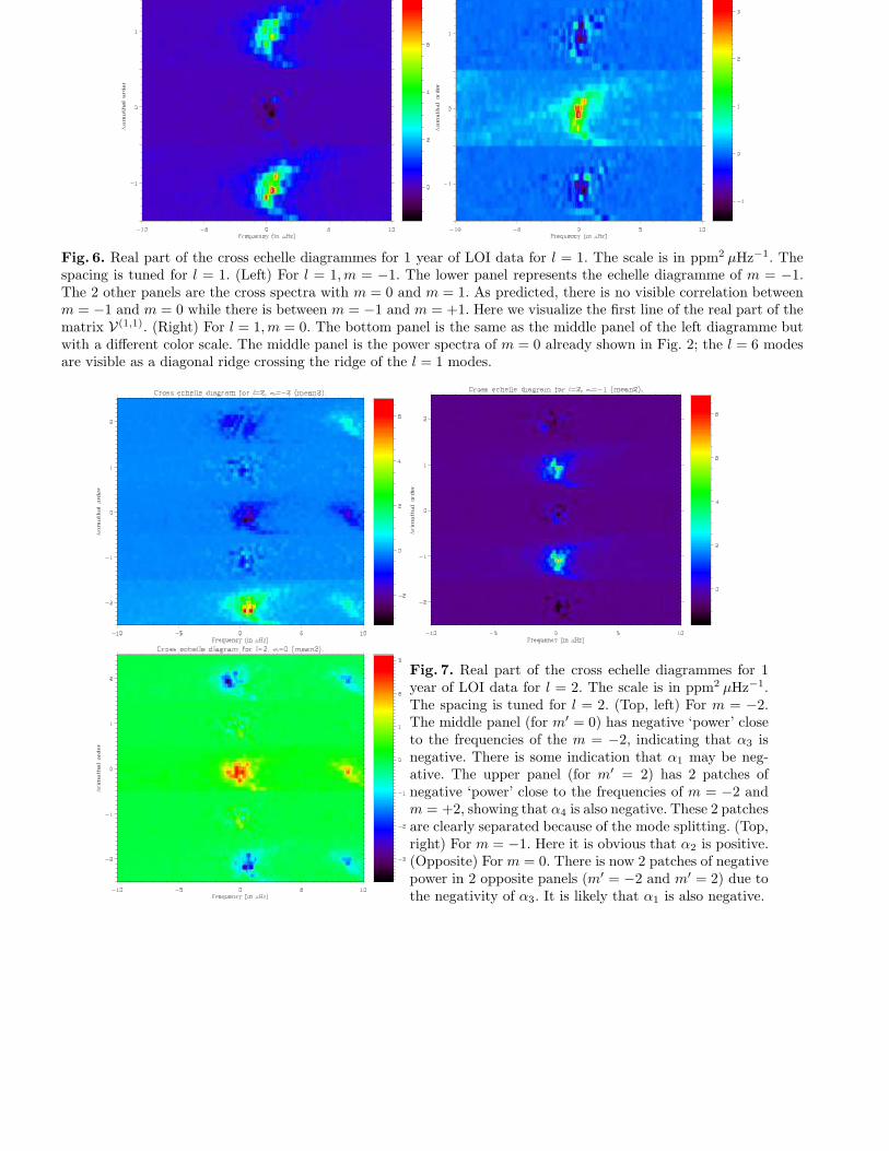
Fig. 6. Real part of the cross echelle diagrammes for 1 year of LOI data for l = 1. The scale is in ppm2 µHz−1. Thespacing is tuned for l = 1. (Left) For l = 1, m = −1. The lower panel represents the echelle diagramme of m = −1.The 2 other panels are the cross spectra with m = 0 and m = 1. As predicted, there is no visible correlation betweenm = −1 and m = 0 while there is between m = −1 and m = +1. Here we visualize the first line of the real part of thematrix V(1,1). (Right) For l = 1, m = 0. The bottom panel is the same as the middle panel of the left diagramme butwith a different color scale. The middle panel is the power spectra of m = 0 already shown in Fig. 2; the l = 6 modesare visible as a diagonal ridge crossing the ridge of the l = 1 modes.

Fig. 7. Real part of the cross echelle diagrammes for 1year of LOI data for l = 2. The scale is in ppm2 µHz−1.The spacing is tuned for l = 2. (Top, left) For m = −2.The middle panel (for m′ = 0) has negative ‘power’ closeto the frequencies of the m = −2, indicating that α3 isnegative. There is some indication that α1 may be neg-ative. The upper panel (for m′ = 2) has 2 patches ofnegative ‘power’ close to the frequencies of m = −2 andm = +2, showing that α4 is also negative. These 2 patchesare clearly separated because of the mode splitting. (Top,right) For m = −1. Here it is obvious that α2 is positive.(Opposite) For m = 0. There is now 2 patches of negativepower in 2 opposite panels (m′ = −2 and m′ = 2) due tothe negativity of α3. It is likely that α1 is also negative.

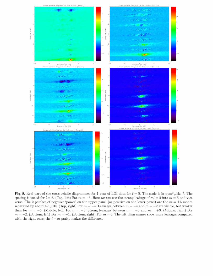
Fig. 8. Real part of the cross echelle diagrammes for 1 year of LOI data for l = 5. The scale is in ppm2 µHz−1. Thespacing is tuned for l = 5. (Top, left) For m = −5. Here we can see the strong leakage of m′ = 5 into m = 5 and viceversa. The 2 patches of negative ‘power’ on the upper panel (or positive on the lower panel) are the m = ±5 modesseparated by about 4-5 µHz. (Top, right) For m = −4. Leakages between m = −4 and m = −2 are visible, but weakerthan for m = −5. (Middle, left) For m = −3. Strong leakages between m = −3 and m = +3. (Middle, right) Form = −2. (Bottom, left) For m = −1. (Bottom, right) For m = 0. The left diagrammes show more leakages comparedwith the right ones, the l + m parity makes the difference.

Fig. 9. Real part of the cross echelle diagrammes of 1 year of LOI data for l = 1. The scale is in ppm2µHz−1. Theinverse of the theoretical leakage matrix has been applied to the original data with α=0.474. (Left) For l = 1, m = −1.The artificial correlation between m = −1 and m = +1 has been entirely removed (See Fig. 6 for comparison). (Right)For l = 1, m = 0. There is no improvement as there was no correlation before.

Fig. 10. Real part of the cross echelle diagrammes of 1year of LOI data for l = 2 after having applied the inverseof the leakage matrix. The scale is in ppm2 µHz−1. Thespacing is tuned for l = 2. (Top, left) For m = −2. (Top,right) For m = −1. (Opposite) For m = 0. Using theinverse of the leakage matrix we have removed all artificialcorrelations (See Fig. 7 for comparison). The spectra havebeen cleaned both from the m leaks and from l = 0 modesbecause we used the leakage matrix of l = 2 and l = 0.

12 (Right). When the corrected surface is close to 0, thereis no artificial correlation remaining.

Cleaning the data from artificial correlations has alsobeen done in a different way by Toutain et al. (1998). Us-

ing Singular Value Decomposition, they recomputed pixelfilters for the MDI/LOI proxy so as to remove the m leaksand the other aliasing degrees. Here we have shown, thatdata cleaning is also possible without having the pixel time

series, but using the Fourier spectra. This latter cleaningtechnique is more useful as one has to reduce a smalleramount of data.

3.4. Leakage matrix measurement for many degrees

3.4.1. LOI/SOHO data

Figures 13 and 14 shows the inter echelle diagramme forl = 1, l′ = 6, and l = 5, l′ = 8, respectively. These di-agrammes are more difficult to interpret, but using spe-cific spacing for l or l′, one can unambiguously identifywhich degree contributes to the correlation. For the LOIdata, the l = 5 and l = 8 (similarly l = 4 and l = 7)are contaminated by each other. This is again due to thespatial undersampling which prevents the LOI data to becleaned from aliasing degrees making the leakage matrixnot invertible. Fortunately, the l = 1 LOI data are farless affected by the presence of l = 6 compared with thatof GONG (See in the next section); this is the result ofan effective apodization function (limb darkening) whichcreates a narrower spatial response than that of GONG(line-of-sight projection).

Figure 10 has already shown that we could clean thel = 2 LOI data from the l = 0 mode. This was doneby taking into account the leakage matrix C(0,2). Unfortu-nately as mentioned for the l = 5, the LOI data cannot becleaned from aliasing degrees because the leakage matriceC(1,6), C(4,7) and C(5,8) are singular.

3.4.2. GONG data

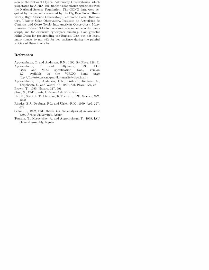
Figures 15 and 17 show the inter echelle diagramme forl = 1, l′ = 6, and for l = 1, l′ = 9. The correlations areclearly visible. If they are not taken into account they arelikely to bias the frequency and splittings of the l = 1(See Rabello-Soares and Appourchaux, 1998, in prepara-tion). By using the inverse full leakage matrix of l = 1, 6and 9 (i.e. C(1,6,9), one can clean the data from these spuri-ous correlations arising both from the aliasing degrees andfrom the m leaks. Figures 16 and 18 shows the ’cleaned’inter echelle diagramme which should be compared withFigs. 15 and 17, respectively. The correlations have beenalmost entirely removed. Some correlations between thel = 1, m = −1 modes and the l = 6, 9 modes are stillpresent. This is due to the fact that the computation ofthe leakage for l = 1, m = ±1 are very sensitive to thesubtraction of the velocity of the Sun seen as a star. Thisis not the case for the l = 1, m = 0 modes as they are in-sensitive to this effect. Nevertheless, our imperfect knowl-edge of the leakage matrix can be adjusted in order toremove the residual correlations. It helped to reduce the

systematic errors of the l = 1 splitting at high frequen-cies, mainly where the l = 6 start to cross over the l = 1(Rabello-Soares and Appourchaux 1998, in preparation).

It is possible to apply this cleaning technique to higherdegree modes (l ≈ 50 − 100. In principle, this is feasible,although the plethora of data involved may be fairly sub-stantial. For higher degrees, the ridges of the modes inthe (m, ν) echelle diagrammes are almost parallel to eachother. The idea would be not to use the full Fourier spec-tra, as we did for the low degree GONG data, but to useonly a small frequency range of about ± 30 µHz aroundthe target degree. By doing so, we will not only clean thedata from the aliasing degrees but also from the m leaks.In this case, the mode covariance matrix is diagonal. If weassume, wrongly, that the noise covariance matrix is diag-onal, the statistics of each cleaned spectrum, for high de-gree modes, could be approximated by a χ2 with 2 degreeof freedom. Neglecting the off-diagonal elements of thenoise covariance matrix will lead to larger mode linewidth,thereby producing underestimated splittings; this system-atic bias will decrease as the degree. This approximationwill produce much less systematic errors than the approx-imation used by Hill et al. (1996) for the original data.The use of the suggested approximation for the GONGdata may help, at the same time, to reduce systematicerrors, and to increase computing speed for higher degreemodes. The degree where one needs to switch betweenthis approximation and the correct analysis needs to bedetermined.

3.5. Noise covariance matrix measurement

3.5.1. LOI/SOHO data

The leakage and ratio matrices have similar properties(See Part I). For example, for a given l there is no cor-relation between the m for which m + m′ is odd for ei-ther matrix. This lack of correlation can be seen in Fig.19 for the ratio cross spectra of the LOI data. The ratiomatrix is also useful if one wants to reduce the number ofnoise parameters to be fitted. This is useful when the noisebackground, mainly of solar origin, varies slowly over thep-mode range. In this case the ratio can be assumed to beconstant over the p-mode range. For example for l = 1 wecan fit 2 noise parameters instead of 3. When the noisevaries in the p-mode range, it is more advisable to fit asmany noise parameters as required.

Figure 20 shows the ratio cross spectra of l = 2 for theLOI data. As this is commonly the case for the LOI, theratios are independent of frequency. In addition, as out-lined in Part I, the ratio matrix is very close to the leakagematrix. Using the values of α given for the LOI in Eq. (11)and Fig. 20, one can see that this is the case for the LOI.The ratio matrix has even the same symmetry property as

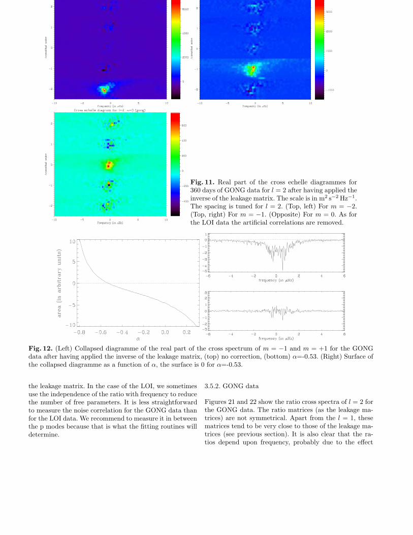
Fig. 11. Real part of the cross echelle diagrammes for360 days of GONG data for l = 2 after having applied theinverse of the leakage matrix. The scale is in m2 s−2 Hz−1.The spacing is tuned for l = 2. (Top, left) For m = −2.(Top, right) For m = −1. (Opposite) For m = 0. As forthe LOI data the artificial correlations are removed.

Fig. 12. (Left) Collapsed diagramme of the real part of the cross spectrum of m = −1 and m = +1 for the GONGdata after having applied the inverse of the leakage matrix, (top) no correction, (bottom) α=-0.53. (Right) Surface ofthe collapsed diagramme as a function of α, the surface is 0 for α=-0.53.

the leakage matrix. In the case of the LOI, we sometimesuse the independence of the ratio with frequency to reducethe number of free parameters. It is less straightforwardto measure the noise correlation for the GONG data thanfor the LOI data. We recommend to measure it in betweenthe p modes because that is what the fitting routines willdetermine.

3.5.2. GONG data

Figures 21 and 22 show the ratio cross spectra of l = 2 forthe GONG data. The ratio matrices (as the leakage ma-trices) are not symmetrical. Apart from the l = 1, thesematrices tend to be very close to those of the leakage ma-trices (see previous section). It is also clear that the ra-tios depend upon frequency, probably due to the effect

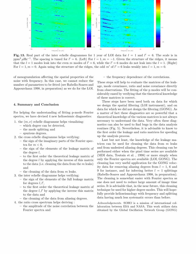
Fig. 13. Real part of the inter echelle diagrammes for 1 year of LOI data for l = 1 and l′ = 6. The scale is inppm2 µHz−1. The spacing is tuned for l′ = 6. (Left) For l = 1, m = −1. Given the structure of the ridges, it meansthat the l = 1 modes leak into the even m modes of l′ = 6, while the l′ = 6 modes do not leak into the l = 1. (Right)For l = 1, m = 0. Again using the structure of the ridges, the odd m′ of l′ = 6 leaks weakly into l = 1, m = 0.

of mesogranulation affecting the spatial properties of thenoise with frequency. In this case, we cannot reduce thenumber of parameters to be fitted (see Rabello-Soares andAppourchaux 1998, in preparation) as we do for the LOI.

4. Summary and Conclusion

For helping the understanding of fitting p-mode Fourierspectra, we have devised 4 new helioseismic diagnostics:

1. the (m, ν) echelle diagramme helps visualizing:– which degree can be detected,– the mode splitting and– spurious degrees.

2. the cross echelle diagramme helps verifying:– the sign of the imaginary parts of the Fourier spec-

tra for m < 0,– the sign of the elements of the leakage matrix of

the degree l,– to the first order the theoretical leakage matrix of

the degree l by applying the inverse of this matrixto the data (i.e. cleaning the data from the m leaks)and

– the cleaning of the data from m leaks.3. the inter echelle diagramme helps verifying:

– the sign of the elements of the full leakage matrixfor degrees l, l′,

– to the first order the theoretical leakage matrix ofthe degree l, l′ by applying the inverse this matrixto the data and

– the cleaning of the data from aliasing degrees.4. the ratio cross spectrum helps deriving :

– the amplitude of the noise correlation between theFourier spectra and

– the frequency dependence of the correlations.

These steps will help to evaluate the matrices of the leak-age, mode covariance, ratio and noise covariance directlyfrom observations. The fitting of the p modes will be con-siderably eased by verifying that the theoretical knowledgeof these matrices is correct.

These steps have been used both on data for whichwe design the spatial filtering (LOI instrument), and ondata for which we did not design the filtering (GONG). Asa matter of fact these diagnostics are so powerful that atheoretical knowledge of the various matrices is not alwaysnecessary to understand the data. Very often these diag-nostics can also be used to find bugs in the data analysisroutines (Fig. 5). Nevertheless, it is advisable to know tothe first order the leakage and ratio matrices for speedingup the analysis process.

Last but not least, the knowledge of the leakage ma-trices can be used for cleaning the data from m leaksand from undesired aliasing degrees. This cleaning can beperformed either when the pixel time series are available(MDI data, Toutain et al. , 1998) or more simply whenonly the Fourier spectra are available (LOI, GONG). Thecleaning has very useful application for the GONG veloc-ity data for removing aliasing degrees from l = 1, 6 and9 for instance, and for inferring better l = 1 splittings(Rabello-Soares and Appourchaux 1998, in preparation).The cleaning is somewhat easier with Fourier spectra asone does not need to reduce large amount of image timeseries. It is advisable that, in the near future, this cleaningtechnique be used for higher degree modes. This will hope-fully provide helioseismology with frequency and splittingdata having much less systematic errors than before.

Acknowledgements. SOHO is a mission of international col-laboration between ESA and NASA. This work utilizes dataobtained by the Global Oscillation Network Group (GONG)

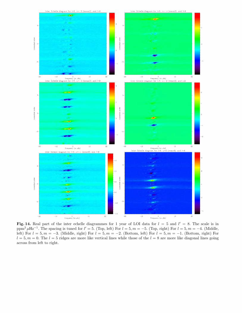
Fig. 14. Real part of the inter echelle diagrammes for 1 year of LOI data for l = 5 and l′ = 8. The scale is inppm2 µHz−1. The spacing is tuned for l′ = 5. (Top, left) For l = 5, m = −5. (Top, right) For l = 5, m = −4. (Middle,left) For l = 5, m = −3. (Middle, right) For l = 5, m = −2. (Bottom, left) For l = 5, m = −1. (Bottom, right) Forl = 5, m = 0. The l = 5 ridges are more like vertical lines while those of the l = 8 are more like diagonal lines goingacross from left to right.

project managed by the National Solar Observatory, a Divi-sion of the National Optical Astronomy Observatories, whichis operated by AURA, Inc. under a cooperative agreement withthe National Science Foundation. The GONG data were ac-quired by instruments operated by the Big Bear Solar Obser-vatory, High Altitude Observatory, Learmonth Solar Observa-tory, Udaipur Solar Observatory, Instituto de Astrofisico deCanarias and Cerro Tololo Interamerican Observatory. Manythanks to Takashi Sekii for constructive comments on the manu-script, and for extensive cyberspace chatting. I am gratefulMihir Desai for proofreading the English. Last but not least,many thanks to my wife for her patience during the painfulwriting of these 2 articles.

References

Appourchaux, T. and Andersen, B.N., 1990, Sol.Phys. 128, 91Appourchaux, T. and Telljohann, 1996, LOI

GSE and VDC specification Doc., Version1.7, available on the VIRGO home page(ftp://ftp.estec.esa.nl/pub/loitenerife/virgo.html)

Appourchaux, T., Andersen, B.N., Frohlich, Jimenez, A.,Telljohann, U. and Wehrli, C., 1997, Sol. Phys., 170, 27

Brown, T., 1985, Nature, 317, 591Grec, G., PhD thesis, Universite de Nice, NiceHill, F., Stark, R.T., Stebbins, R.T. et al. , 1996, Science, 272,

1292Rhodes, E.J., Deubner, F-L. and Ulrich, R.K., 1979, ApJ, 227,

629Schou, J., 1992, PhD thesis, On the analysis of helioseismic

data, Arhus Universitet, ArhusToutain, T., Kosovichev, A. and Appourchaux, T., 1998, IAU

General assembly, Kyoto

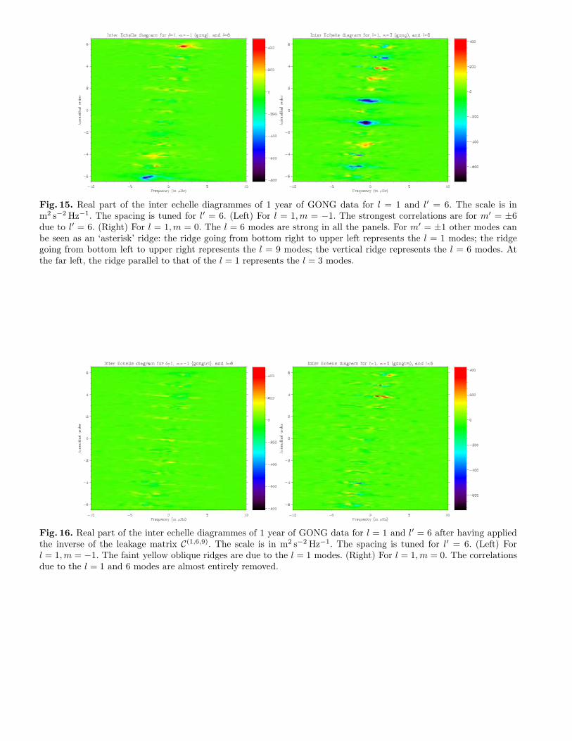
Fig. 15. Real part of the inter echelle diagrammes of 1 year of GONG data for l = 1 and l′ = 6. The scale is inm2 s−2 Hz−1. The spacing is tuned for l′ = 6. (Left) For l = 1, m = −1. The strongest correlations are for m′ = ±6due to l′ = 6. (Right) For l = 1, m = 0. The l = 6 modes are strong in all the panels. For m′ = ±1 other modes canbe seen as an ‘asterisk’ ridge: the ridge going from bottom right to upper left represents the l = 1 modes; the ridgegoing from bottom left to upper right represents the l = 9 modes; the vertical ridge represents the l = 6 modes. Atthe far left, the ridge parallel to that of the l = 1 represents the l = 3 modes.

Fig. 16. Real part of the inter echelle diagrammes of 1 year of GONG data for l = 1 and l′ = 6 after having appliedthe inverse of the leakage matrix C(1,6,9). The scale is in m2 s−2 Hz−1. The spacing is tuned for l′ = 6. (Left) Forl = 1, m = −1. The faint yellow oblique ridges are due to the l = 1 modes. (Right) For l = 1, m = 0. The correlationsdue to the l = 1 and 6 modes are almost entirely removed.

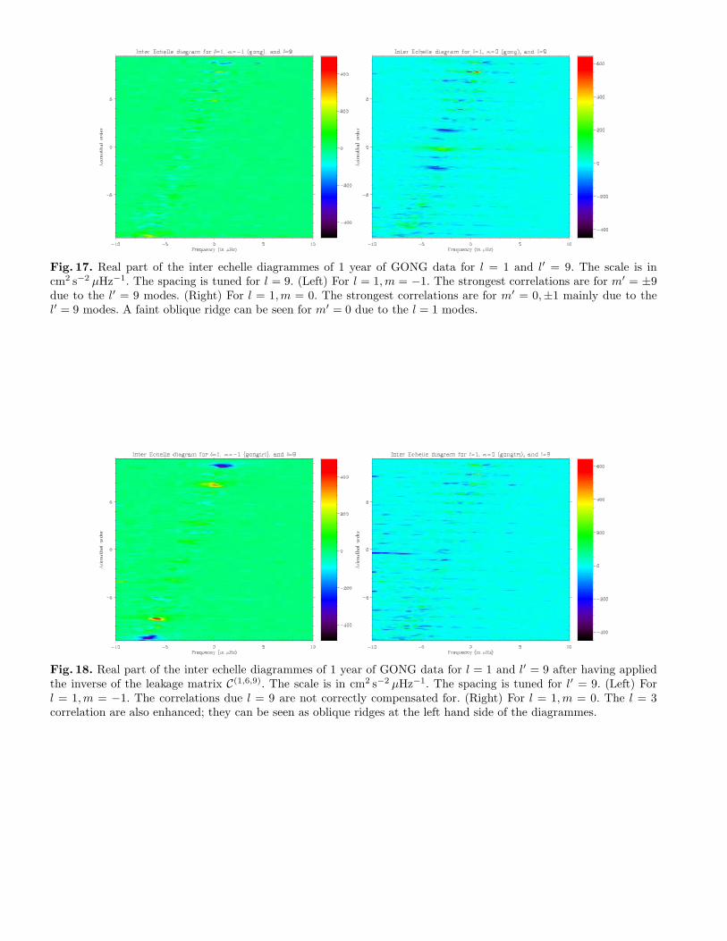
Fig. 17. Real part of the inter echelle diagrammes of 1 year of GONG data for l = 1 and l′ = 9. The scale is incm2 s−2 µHz−1. The spacing is tuned for l = 9. (Left) For l = 1, m = −1. The strongest correlations are for m′ = ±9due to the l′ = 9 modes. (Right) For l = 1, m = 0. The strongest correlations are for m′ = 0,±1 mainly due to thel′ = 9 modes. A faint oblique ridge can be seen for m′ = 0 due to the l = 1 modes.

Fig. 18. Real part of the inter echelle diagrammes of 1 year of GONG data for l = 1 and l′ = 9 after having appliedthe inverse of the leakage matrix C(1,6,9). The scale is in cm2 s−2 µHz−1. The spacing is tuned for l′ = 9. (Left) Forl = 1, m = −1. The correlations due l = 9 are not correctly compensated for. (Right) For l = 1, m = 0. The l = 3correlation are also enhanced; they can be seen as oblique ridges at the left hand side of the diagrammes.

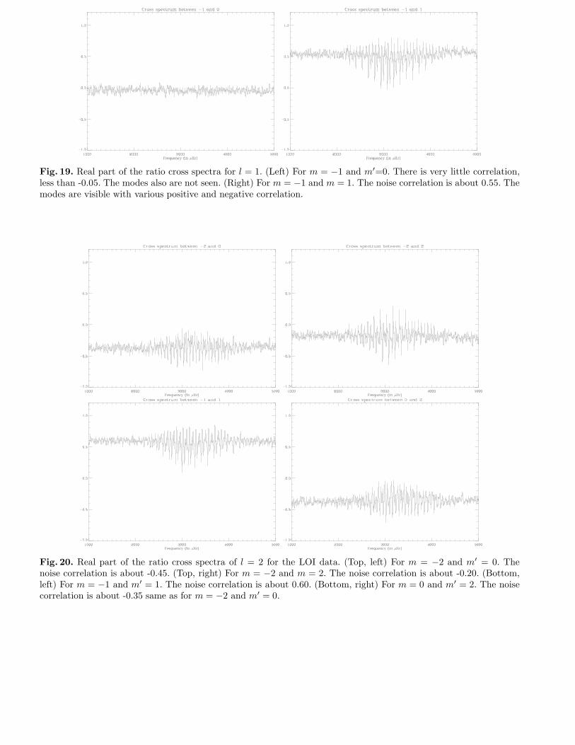
Fig. 19. Real part of the ratio cross spectra for l = 1. (Left) For m = −1 and m′=0. There is very little correlation,less than -0.05. The modes also are not seen. (Right) For m = −1 and m = 1. The noise correlation is about 0.55. Themodes are visible with various positive and negative correlation.

Fig. 20. Real part of the ratio cross spectra of l = 2 for the LOI data. (Top, left) For m = −2 and m′ = 0. Thenoise correlation is about -0.45. (Top, right) For m = −2 and m = 2. The noise correlation is about -0.20. (Bottom,left) For m = −1 and m′ = 1. The noise correlation is about 0.60. (Bottom, right) For m = 0 and m′ = 2. The noisecorrelation is about -0.35 same as for m = −2 and m′ = 0.

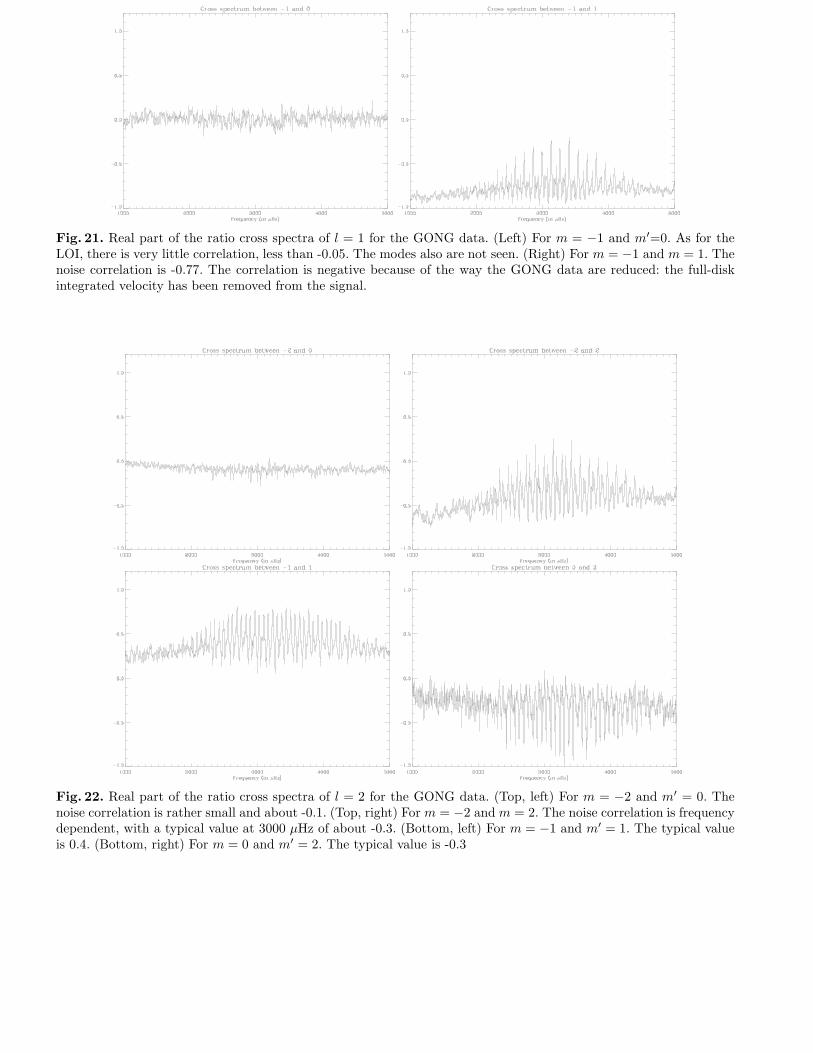
Fig. 21. Real part of the ratio cross spectra of l = 1 for the GONG data. (Left) For m = −1 and m′=0. As for theLOI, there is very little correlation, less than -0.05. The modes also are not seen. (Right) For m = −1 and m = 1. Thenoise correlation is -0.77. The correlation is negative because of the way the GONG data are reduced: the full-diskintegrated velocity has been removed from the signal.

Fig. 22. Real part of the ratio cross spectra of l = 2 for the GONG data. (Top, left) For m = −2 and m′ = 0. Thenoise correlation is rather small and about -0.1. (Top, right) For m = −2 and m = 2. The noise correlation is frequencydependent, with a typical value at 3000 µHz of about -0.3. (Bottom, left) For m = −1 and m′ = 1. The typical valueis 0.4. (Bottom, right) For m = 0 and m′ = 2. The typical value is -0.3