This content has been downloaded from IOPscience. Please scroll down to see the full text.

Download details:

IP Address: 110.4.24.170

This content was downloaded on 14/10/2013 at 16:25

Please note that terms and conditions apply.

The B-spline R-matrix method for atomic processes: application to atomic structure, electron

collisions and photoionization

View the table of contents for this issue, or go to the journal homepage for more

2013 J. Phys. B: At. Mol. Opt. Phys. 46 112001

(http://iopscience.iop.org/0953-4075/46/11/112001)

Home Search Collections Journals About Contact us My IOPscience

IOP PUBLISHING JOURNAL OF PHYSICS B: ATOMIC, MOLECULAR AND OPTICAL PHYSICS

J. Phys. B: At. Mol. Opt. Phys. 46 (2013) 112001 (39pp) doi:10.1088/0953-4075/46/11/112001

TOPICAL REVIEW

The B-spline R-matrix method for atomicprocesses: application to atomic structure,electron collisions and photoionizationOleg Zatsarinny and Klaus Bartschat

Department of Physics and Astronomy, Drake University, Des Moines, IA 50311, USA

E-mail: oleg.zatsarinny@drake.edu and klaus.bartschat@drake.edu

Received 17 February 2013, in final form 10 April 2013Published 9 May 2013Online at stacks.iop.org/JPhysB/46/112001

AbstractThe basic ideas of the B-spline R-matrix (BSR) approach are reviewed, and the use of themethod is illustrated with a variety of applications to atomic structure, electron–atomcollisions and photo-induced processes. Special emphasis is placed on complex, open-shelltargets, for which the method has proven very successful in reproducing, for example, a wealthof near-threshold resonance structures. Recent extensions to a fully relativistic framework andintermediate energies have allowed for an accurate treatment of heavy targets as well as a fullynonperturbative scheme for electron-impact ionization. Finally, field-free BSR Hamiltonianand electric dipole matrices can be employed in the time-dependent treatment of intenseshort-pulse laser–atom interactions.

(Some figures may appear in colour only in the online journal)

1. Introduction

Over the past decades, a number of general computer codeshave been developed to generate accurate data for atomicand molecular structure, as well as electron and photoncollisions with atoms, ions and molecules. Theoretical andcomputational work in this area is supporting many ongoingexperiments, providing not only insight at the fundamentallevel of submicroscopic, often highly correlated quantummechanical few-body systems, but also data needed in manypractical applications, such as modelling the behaviour ofvarious plasmas and discharges as well as diagnosing theirproperties. Numerous calculations have been performed overthe past decades, with rapidly increasing complexity in thelight of the fact that computational resources have becomeabundant. Comparison with experimental benchmark data,of course, remains necessary to validate the theoreticalpredictions, thereby providing some confidence in the use oftheoretical numbers, especially when theory is the only sourceof sufficiently complete datasets.

This topical review is devoted to one recently (since about2000) developed method, namely the B-Spline R-matrix (BSR)approach. It is one of many that can, in principle, be usedto solve the so-called close-coupling equations. As will beillustrated below, the BSR method has been employed verysuccessfully for a number of atomic structure calculations,but especially for the treatment of electron-induced processes(elastic scattering, excitation, de-excitation, ionization), andthe interaction of weak (generally continuous) and strong(usually pulsed) electromagnetic fields with atoms and atomicions (positive and negative). All these processes can behandled with the same basic over-arching approach, with theappropriate details being implemented through the boundaryconditions for the close-coupling equations and the extent towhich various physical phenomena (e.g., electron correlations,relativistic effects, channel coupling) are accounted for. Whilethe method can be further developed towards molecules, wewill exclusively deal with atomic targets here.

A summary of BSR-related publications is providedin tables 1−4. Table 1 lists a number of write-ups andmethodology papers, including the publicly available suite of

0953-4075/13/112001+39$33.00 1 © 2013 IOP Publishing Ltd Printed in the UK & the USA

J. Phys. B: At. Mol. Opt. Phys. 46 (2013) 112001 Topical Review

Table 1. List of BSR programs and write-ups (2000–present).

Topic Remarks Reference

Write-up Nonrelativistic + Breit–Pauli [1](Some programs) Structure calculations [2]

B-splines for DBSR [3]Angular integrals in nonorthogonal [4]basisTime-dependent BSR approach [5]

Table 2. List of BSR publications for atomic structure(2000–present).

Topic Target Reference

Rydberg series C [6]Oscillator strengths Ne [7]

S [8]S II [9]Ar [7, 10]Kr [7]Xe [7, 11]

Polarizabilities F [12]Cl [13]

codes [1] that was used in many of the early works listed intable 2 for atomic structure calculations, table 3 for electroncollisions and table 4 for radiative processes. Over the past fewyears, however, significant further progress has been achieved,including the development of a fully relativistic Dirac-based(DBSR) version, the inclusion of a large number of pseudo-states that allow for coupling to the ionization continuum and,ultimately, the fully nonperturbative treatment of ionizationprocesses, and the use of field-free Hamiltonian and dipolematrices from the BSR complex in the solution of the time-dependent Schrodinger equation (TDSE) for intense short-pulse laser–atom interactions.

As seen from the tables, the (D)BSR method is veryversatile. While many test calculations were performedfor relatively simple quasi-one-electron (hydrogen-like) andquasi-two-electron (helium-like) targets, the method isparticularly suitable when the complexity of the target isincreased, and especially when the coupling of anotherelectron is required to properly describe an electron collisionprocess. Consequently, it has enjoyed the largest success indealing with complex open-shell targets.

The two most significant innovations of the BSR approachcompared to other methods and the accompanying computercodes are the following:

(i) Different sets of nonorthogonal orbitals can be used torepresent both the bound and continuum one-electronorbitals.

(ii) A set of B-splines defines the R-matrix basis functions.

The use of nonorthogonal bound orbital sets allows fora much higher accuracy in the description of the targetstates than what is typically achieved when orthogonalityis enforced. Since the orbitals are optimized in separatecalculations for individual terms, a high level of accuracycan be obtained with compact configuration interaction (CI)expansions. Regarding the close-coupling expansion of the

Table 3. List of BSR publications for electron collisions(2000–present).

Topic Target Remarks Reference

e–ion collisions Fe II [14]Fe VIII [15]S II [9]K II [16, 17]

e–neutral collisions He [18–20](Discrete states, C [21]excitation) N [22]

O [23–26]S [27, 28]Cl [29]Ne [30–33]Ne Plasma modelling [34, 35]Na Autoionizing levels [36, 37]Mg [38]Si [39]Ar [40, 41]Ar Plasma modelling [42–44]K Autoionizing levels [45, 46]Ca [47, 48]Cu [49, 50]Zn [51–53]I [54]Kr [55–57, 44]Rb Autoionizing levels [58]Xe [41]Xe Plasma modelling [59]Cs Autoionizing levels [60]Kr DBSR [61]Xe DBSR [61]Cs DBSR [62]Au DBSR [63, 64]Hg DBSR [65–67]Pb DBSR [68, 69]

e-neutral collisions He [70, 71](Large RMPS, C [72]incl. ionization) Ne [73–75]

Ar [76, 77]

Table 4. List of BSR publications for photo-induced processes(2000–present).

Topic Target Remarks Reference

Photodetachment He− (1s2s2p)4Po [78]Li− [79]B− [80]O− [81]Ca− [48]

Weak-field Li [25]photoionization K [82]

Zn [83]Strong-field He Double ionization [84]photoionization Ne Single ionization [85]

Ar Single ionization [86]

total wavefunction for collision problems, certain (N + 1)-electron bound configurations must often be included tocompensate for orthogonality constraints imposed on thecontinuum orbitals. However, it can be difficult to keep theexpansion fully consistent, and any inconsistency may lead to apseudo-resonance structure. Using nonorthogonal continuumorbitals, on the other hand, avoids the introduction of these

2

J. Phys. B: At. Mol. Opt. Phys. 46 (2013) 112001 Topical Review

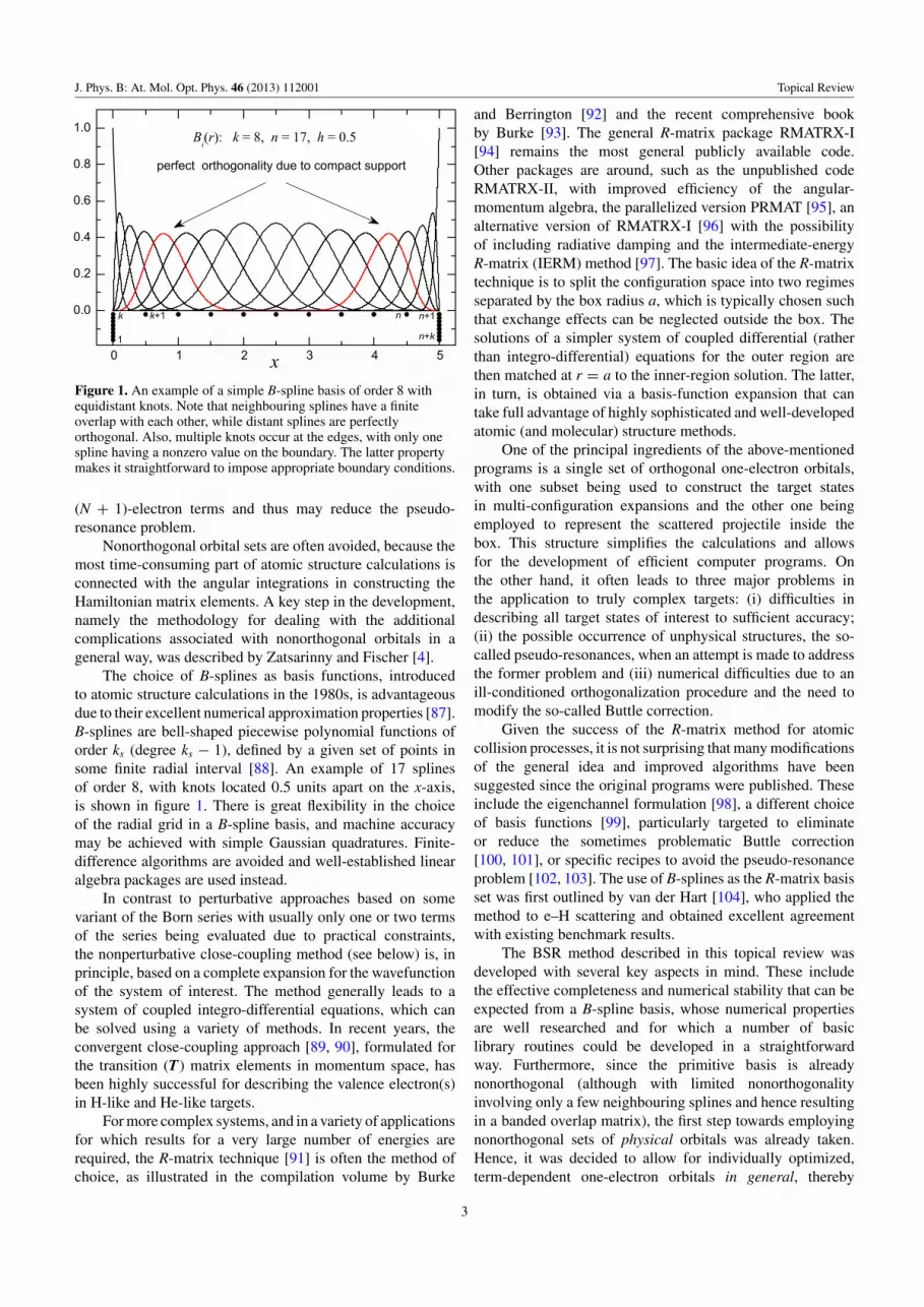
Figure 1. An example of a simple B-spline basis of order 8 withequidistant knots. Note that neighbouring splines have a finiteoverlap with each other, while distant splines are perfectlyorthogonal. Also, multiple knots occur at the edges, with only onespline having a nonzero value on the boundary. The latter propertymakes it straightforward to impose appropriate boundary conditions.

(N + 1)-electron terms and thus may reduce the pseudo-resonance problem.

Nonorthogonal orbital sets are often avoided, because themost time-consuming part of atomic structure calculations isconnected with the angular integrations in constructing theHamiltonian matrix elements. A key step in the development,namely the methodology for dealing with the additionalcomplications associated with nonorthogonal orbitals in ageneral way, was described by Zatsarinny and Fischer [4].

The choice of B-splines as basis functions, introducedto atomic structure calculations in the 1980s, is advantageousdue to their excellent numerical approximation properties [87].B-splines are bell-shaped piecewise polynomial functions oforder ks (degree ks − 1), defined by a given set of points insome finite radial interval [88]. An example of 17 splinesof order 8, with knots located 0.5 units apart on the x-axis,is shown in figure 1. There is great flexibility in the choiceof the radial grid in a B-spline basis, and machine accuracymay be achieved with simple Gaussian quadratures. Finite-difference algorithms are avoided and well-established linearalgebra packages are used instead.

In contrast to perturbative approaches based on somevariant of the Born series with usually only one or two termsof the series being evaluated due to practical constraints,the nonperturbative close-coupling method (see below) is, inprinciple, based on a complete expansion for the wavefunctionof the system of interest. The method generally leads to asystem of coupled integro-differential equations, which canbe solved using a variety of methods. In recent years, theconvergent close-coupling approach [89, 90], formulated forthe transition (T) matrix elements in momentum space, hasbeen highly successful for describing the valence electron(s)in H-like and He-like targets.

For more complex systems, and in a variety of applicationsfor which results for a very large number of energies arerequired, the R-matrix technique [91] is often the method ofchoice, as illustrated in the compilation volume by Burke

and Berrington [92] and the recent comprehensive bookby Burke [93]. The general R-matrix package RMATRX-I[94] remains the most general publicly available code.Other packages are around, such as the unpublished codeRMATRX-II, with improved efficiency of the angular-momentum algebra, the parallelized version PRMAT [95], analternative version of RMATRX-I [96] with the possibilityof including radiative damping and the intermediate-energyR-matrix (IERM) method [97]. The basic idea of the R-matrixtechnique is to split the configuration space into two regimesseparated by the box radius a, which is typically chosen suchthat exchange effects can be neglected outside the box. Thesolutions of a simpler system of coupled differential (ratherthan integro-differential) equations for the outer region arethen matched at r = a to the inner-region solution. The latter,in turn, is obtained via a basis-function expansion that cantake full advantage of highly sophisticated and well-developedatomic (and molecular) structure methods.

One of the principal ingredients of the above-mentionedprograms is a single set of orthogonal one-electron orbitals,with one subset being used to construct the target statesin multi-configuration expansions and the other one beingemployed to represent the scattered projectile inside thebox. This structure simplifies the calculations and allowsfor the development of efficient computer programs. Onthe other hand, it often leads to three major problems inthe application to truly complex targets: (i) difficulties indescribing all target states of interest to sufficient accuracy;(ii) the possible occurrence of unphysical structures, the so-called pseudo-resonances, when an attempt is made to addressthe former problem and (iii) numerical difficulties due to anill-conditioned orthogonalization procedure and the need tomodify the so-called Buttle correction.

Given the success of the R-matrix method for atomiccollision processes, it is not surprising that many modificationsof the general idea and improved algorithms have beensuggested since the original programs were published. Theseinclude the eigenchannel formulation [98], a different choiceof basis functions [99], particularly targeted to eliminateor reduce the sometimes problematic Buttle correction[100, 101], or specific recipes to avoid the pseudo-resonanceproblem [102, 103]. The use of B-splines as the R-matrix basisset was first outlined by van der Hart [104], who applied themethod to e–H scattering and obtained excellent agreementwith existing benchmark results.

The BSR method described in this topical review wasdeveloped with several key aspects in mind. These includethe effective completeness and numerical stability that can beexpected from a B-spline basis, whose numerical propertiesare well researched and for which a number of basiclibrary routines could be developed in a straightforwardway. Furthermore, since the primitive basis is alreadynonorthogonal (although with limited nonorthogonalityinvolving only a few neighbouring splines and hence resultingin a banded overlap matrix), the first step towards employingnonorthogonal sets of physical orbitals was already taken.Hence, it was decided to allow for individually optimized,term-dependent one-electron orbitals in general, thereby

3

J. Phys. B: At. Mol. Opt. Phys. 46 (2013) 112001 Topical Review

taking advantage of compact configuration expansions togenerate accurate wavefunctions for the N-electron targetand, if needed, the (N + 1)-electron collision system andespecially its resonances. Finally, the package was supposedto be general, allowing for structure calculations as wellas the treatment of electron and photon-induced processes.Relativistic effects can be accounted for with the appropriatedegree of accuracy, and the treatment of electron-impactionization has become possible via the introduction of a largenumber of so-called pseudo-states that effectively provide adiscretization of the target continuum via quasi-bound states.Finally, an extension towards the treatment of time-dependentprocesses was desirable as well.

This topical review is organized as follows. After thisintroduction, section 2 describes the basic ingredients of theBSR method. (Readers who are mainly interested in gettingan impression of possible applications of the method couldskip this section.) Starting with the close-coupling expansion,we introduce the R-matrix methodology in the inner region,the matching to the solution outside the box, the descriptionof bound states rather than collisions and the calculation ofradiative processes. This is followed by the treatment ofrelativistic effects, coupling to the ionization continuum,which allows for a fully nonperturbative description ofionization processes, and another extension dealing with time-dependent processes. Section 3 is devoted to illustrationthrough a collection of sample results, ranging from atomicstructure to electron scattering and photo-induced processes.While we will attempt to keep the review self-contained, spacelimitations require the omission of many details. The interestedreader is thus referred to the original references listed intables 1−4. We finish with a summary, conclusions, and anoutlook in section 4.

Unless specified otherwise, atomic units (au) are usedthroughout this manuscript.

2. General theory

2.1. The close-coupling expansion

The problem of low-energy electron scattering from an N-electronic atomic target is reduced to solving the time-independent Schrodinger equation

(HN+1 − E )�α(�X, xN+1) = 0 (1)

with appropriate boundary conditions. The collisionwavefunction �α(�X ,xN+1) represents a fully antisym-metrized wavefunction of the system ‘target atom + projec-tile electron’, where X ≡ (x1,x2, . . . , xN) and xi≡ (ri,σ i), withthe spatial (ri) and spin (σ i) coordinates of the ith electron.Furthermore, � is a complete set of quantum numbers of the(N + 1)-electron system, and E is the total energy. The sub-script α characterizes the initial conditions and usually denotesthe incoming scattering channel.

The Hamiltonian HN+1, which describes the scatteringof an electron from an N-electron atomic target with nuclearcharge Z, has the form

HN+1 =N+1∑i=1

(−1

2∇2

i − Z

ri

)+

N+1∑i> j=1

1

ri j, (2)

where ri j = |ri − r j|, with ri and r j denoting the vectorcoordinates of electrons i and j. The origin of the coordinateframe is set at the target nucleus, which is assumed to havean infinite mass. For the time being we neglect all relativisticeffects in order to simplify the notation. We introduce a set oftarget states, including possible pseudo-states �i (see below),and their corresponding eigenenergies Ei by the equation

〈�i|HN |� j〉 = Ei(Z, N) δi j, (3)

where the integration is carried out over all the space and spincoordinates of the target electrons. Then the total energy in acollision process is E = Ei + k2

i /2, with Ei being the energyof the target in the state i, while ki

2/2 represents the kineticenergy of the projectile electron. The target states are expandedin terms of single-configuration basis states ϕ j by

�i(x1, . . . , xN ) =∑

j

ϕ j(x1, . . . , xN )ci j, (4)

where the coefficients cij are determined by diagonalizingthe target Hamiltonian. The configurations ϕ j are constructedfrom a one-electron bound orbital basis, usually consisting ofphysical self-consistent field orbitals plus possibly additionalpseudo-orbitals. The latter are included to represent correlationeffects. Note that we do not assume the one-electron basis tobe orthogonal, as is often imposed in scattering calculations.This allows us to optimize the bound orbitals in independentcalculations for each target state and thus to use term-dependent one-electron radial functions.

The solution of (1) has to satisfy the boundary conditionsof an incoming wave packet in some scattering channel α

and outgoing waves in this and all other channels. In theclose-coupling approximation, the solution is expanded interms of a set of N-electron target wavefunctions �i. Thecorresponding expansion coefficients play effectively the roleof wavefunctions for the incident electron. In practice, oneuses

��α (x1, . . . , xN+1)

= An∑

i=1

��i (x1, . . . , xN; rN+1, σN+1)

1

rN+1F�

iα (rN+1)

+m∑

j=1

c jχ�j (x1, . . . , xN+1), (5)

where A is the antisymmetrization operator with respect tothe exchange of any pair of electrons while F�

iα (r) is the radialcomponent of the scattered electron wavefunction when thetarget is in the ith state. The index i includes all quantum statesof the system, and �i is a channel function that is obtained bycoupling the target state with the spin-angle functions of thescattered electron. A major question, of course, concerns thecompleteness of the expansion, in particular when it comesto accounting for the ionization continuum. Traditionally, theexpansion was cut off after including only a few discrete, low-lying physical target states, thereby resulting in the methodbeing restricted to the low-energy near-threshold regime.

Next, let us denote the quantum numbers of the incidentelectron by kilimli msi . The Hamiltonian (2) is diagonal withrespect to the total orbital momentum L, total spin S, theirprojections ML and MS onto the chosen axis and the parity π of

4

J. Phys. B: At. Mol. Opt. Phys. 46 (2013) 112001 Topical Review

the total system. Therefore, in the expansion (5) it is convenientto use the coupled angular-momentum representation,in which

� ≡ γ LSMLMSπ, (6)

where γ denotes the set of all other quantum numbers. Thechannel functions � are defined according to the followingcoupling scheme:

��i (x1, . . . , xN; rN+1, σN+1)

=∑

MLi mli

∑MSi mi

(LiMLi , limli |LML)

(SiMSi ,

1

2mi|SMS

)

×�i(x1, . . . , xN )Ylimli(rN+1)χ 1

2 mi(σN+1). (7)

Here Ylm is a spherical harmonic, χ (σ ) is a spin function,and we use the standard notation for the Clebsch–Gordancoefficients. The function F�

iα (xN+1) in (5) for the incidentelectron can describe both open and closed channels. If (E−Ei)

is positive, the channel is said to be ‘open’; otherwise, thechannel is ‘closed’. Note, however, that the function F�

iα (xN+1)

is not quadratically integrable for open channels. Closed-channel radial functions must satisfy the same boundaryconditions at r = 0 and the same orthogonality conditions asthe open-channel functions, but the closed-channel functionsare quadratically integrable.

The first term in expansion (5) should also include theintegration over the continuous spectrum of the target, whichcorresponds to excitation into the ionization continuum. Adirect inclusion of this term in (5) would tremendouslycomplicate the computational problem since the channel indexbecomes a continuous variable and the number of channelsis not countable. Very often, therefore, this term is omittedentirely. However, the continuum part of the close-couplingexpansion was found to be very important at intermediatescattering energies from about the ionization threshold to afew times that threshold. It can be simulated, to some extent,by the inclusion of bound pseudo-states. Employing a largenumber of pseudo-states, therefore, can essentially eliminatethe low-energy restriction of the close-coupling method. Thiswill be discussed below.

The correlation functions χ i are quadratically integrablefunctions, usually constructed from the same set of one-electron orbitals as the target states �i. The correlationfunctions ensure that the expansion (5) is complete inthe bound orbital basis, even when the continuum radialfunctions are chosen to be orthogonal to the boundorbitals.

In the central field approximation, the atomic orbitals arerepresented in the form

ϕ j(x) = Yljmj (r)χ(ms|σ )1

rPnjl j (r). (8)

Then it is usually demanded that for l j =li the orthogonalitycondition ∫ ∞

0Pnjl j (r)Fiα(r) dr = 0 (9)

is satisfied. This condition does not follow from generalprinciples and is introduced only to simplify numericalcalculations. The introduction of the correlation functions

χ j(x1, . . . , xN+1) means that, in spite of implying conditions(9), the second sum in (5) permits us to account for the virtualcapture of electrons into an unfilled subshell.

In our implementation of the BSR method and thecorresponding computer code [1], the conditions (9) areoptional. The use of nonorthogonal continuum orbitals allowsus to avoid the introduction of the correlation functionsχ j(x1, . . . , xN+1), or to use them directly to describe short-range correlations when the convergence of the expansionbecomes too slow. In our case, they can also be generatedindependently from the target states.

Coupled equations for the radial components of thefunctions Fi(r) and the coefficients c j are obtained bysubstituting expansion (5) into the Schrodinger equationand projecting onto the target functions �i and the L2

functions χ i. After separating out the spin and angularvariables and eliminating the coefficients c j, we obtain thefollowing set of coupled integro-differential (‘close-coupling’)equations:(

d2

dr2− li(li + 1)

r2+ 2Z

r+ k2

i

)Fi(r)

= 2∑

j

(Vi j + Wi j + Xi j)Fj(r). (10)

Here li is the orbital angular momentum of the scatteredelectron while Vij, W ij and Xij are the partial-wavedecompositions of the local direct, nonlocal exchange andnonlocal correlation potentials, respectively. These potentialsare too complicated to write down explicitly except forthe simplest atoms. Instead they are constructed by generalcomputer programs. The equations (10) can also contain termsthat arise from the orthogonality constraints on the scatteringradial functions Fi(r).

Over the past decades, many computational methodshave been developed for solving equations (10) to yield thescattering matrices and amplitudes, which can be combinedto calculate observable quantities for comparison withexperiment. These methods form the basis for a number ofcomputer program packages, some of which are widely used.As examples we mention the linear algebraic equation method[105], the noniterative integral equation method [106], theR-matrix method (see below) and again the convergent close-coupling approach [90]. All these methods seek the solutionof equations (10) in either configuration or momentum spacefor each collision energy.

A promising approach for the direct solution of the close-coupling equations (10), based on the B-spline basis andnotable for its simplicity, which is a key to a successfulcomputational implementation, was put forward by Fischerand Idrees [107]. The method determines the requiredsolution within a finite boundary, with no assumed boundaryconditions. This is not a limitation, provided that theasymptotic region is reached, so that the solutions can bematched to a linear combination of true asymptotic solutions.The core of the algorithm involves the evaluation of theHamiltonian and overlap matrix elements in the B-splinebasis,

Hi j = 〈�i, H� j〉, Si j = 〈�i, � j〉, (11)

5

J. Phys. B: At. Mol. Opt. Phys. 46 (2013) 112001 Topical Review

and the extraction of the eigenvectors relative to the minimummodulus eigenvalues of the nonhermitian, energy-dependentmatrix

A(E ) = H − ES (12)

at each prefixed energy E.

2.2. The R-matrix method

As mentioned earlier, the R-matrix method is one of manyfor solving the close-coupling equations (10). A detaileddescription of the method and its many applications canbe found in the recent book by Burke [93]. Here we onlysummarize the basic ideas.

The important difference from the straightforward close-coupling formalism is a separate treatment of two regions: aninner region, in which all the electrons are closely interactingwith each other and possible external fields, and an outerregion, in which the continuum electron only feels a localpotential. Here the coupled equations (with simple long-range potentials) are solved for each collision energy andmatched, at the boundary r = a, to the solution in the innerregion. However, instead of solving a set of coupled integro-differential equations in the internal region for each collisionenergy, the (N+1)-electron wavefunction is expanded in termsof an energy-independent basis set and treated similarlyto electrons in atomic bound states. Consequently, generalcomputer codes written for bound-state atomic structureproblems can be used, with only minor modifications, togenerate the scattering algebra.

In the internal region, the (N+1)-electron wavefunction atenergy E is expanded in terms of an energy-independent basisset, �k, as

��E =

∑k

A�Ek�

�k . (13)

The basis states for a given total angular momenta areconstructed as

��k (x1, . . . , xN+1)

= A∑i, j

��i (x1, . . . , xN; rN+1, σN+1)

1

rN+1u j(rN+1)c

�i jk

+∑

i

χ�i (x1, . . . , xN+1)d

�ik. (14)

The ui in equation (14) are radial continuum basis functionsdescribing the motion of the scattering electron. They arenonzero on the boundary of the internal region and thus providethe link between the solution in the internal and externalregions. The quadratically integrable functions χ i have thesame meaning as in equation (5) and are assumed to be fullyconfined to the internal region. The coefficients c�

i jk and d�ik are

determined below.Consider now the solution of the Schrodinger equation in

the internal region [0,a]. We note that the Hamiltonian HN+1

is not Hermitian in this region due to the surface terms atr = a that arise from the kinetic energy operator. These surfaceterms can be cancelled by introducing the Bloch operator

LN+1 =N+1∑i=1

1

2δ(ri − a)

(d

dri− b − 1

ri

), (15)

where b is an arbitrary constant (often chosen as b = 0). Notethat HN+1+LN+1 is Hermitian for functions satisfying arbitraryboundary conditions at r = a. We then rewrite the Schrodingerequation in the inner region as

(HN+1 + LN+1 − E )� = LN+1�. (16)

This equation can be formally solved in terms of the R-matrixbasis functions �k, which are obtained through⟨

��i

∣∣HN+1 + LN+1

∣∣��j

⟩int = E�

i

⟨��

i

∣∣��j

⟩int, (17)

where the integration over the radial variables is restrictedto the internal region. This generalized eigenvalue problemdetermines the coefficients c�

i jk and d�ik in (13).

The formal solution of equation (17) can be expanded as

|��〉 =∑

k

∣∣��k

⟩ 1

E�k − E

⟨��

k

∣∣LN+1|��〉int. (18)

Projecting this equation onto the channel functions � andevaluating on the boundary of the internal region yields

F�i (a) =

∑j

R�i j(E )

(a

dF�j

dr− bF�

j

)rN+1=a

, (19)

where we have introduced the R-matrix with elements

R�i j(E ) = 1

2a

∑k

w�ikw

�jk

E�k − E

, (20)

the reduced radial wavefunctions

F�i (rN+1) = rN+1

⟨��

i

∣∣��k

⟩′(21)

and the surface amplitudes

w�ik = a

⟨��

i

∣∣��k

⟩′rN+1=a. (22)

The primes on the brackets in equations (21) and (22) indicatethat the integration is carried out over all the electronic spaceand spin coordinates, except for the radial coordinate ofthe scattered electron. Equations (19) and (20) describe thescattering of electrons from atoms or ions in the internal region.Together with the following relations for the coefficients AEk

in (13),

A�Ek = 1

2a(Ek − E )−1

∑i

wik(a)

(a

dF�i

dr− bF�

i

)r=a

= 1

2a(Ek − E )−1wT R−1F�, (23)

they allow us to establish the wavefunction �E in the innerregion for any value of the total energy E given the valuesof the scattering orbitals on the boundary. The R-matrix withelements given by equation (20) is obtained at all energies bydiagonalizing HN+1 +LN+1 for each set of conserved quantumnumbers � to determine the basis functions �k and thecorresponding eigenenergies Ek. The logarithmic derivativesof the continuum radial wavefunctions Fi(r) on the boundaryof the internal region are then given by equation (19).

An important point in the R-matrix method is the choiceof the radial continuum basis functions uj in equation (14).Although members of any complete set of functions satisfyingarbitrary boundary conditions can be used, a careful choicewill speed up the convergence of the expansion (13). In thestandard R-matrix approach developed by the Belfast group

6

J. Phys. B: At. Mol. Opt. Phys. 46 (2013) 112001 Topical Review

[92, 93], numerical basis functions satisfying homogeneousboundary conditions at r = a were adopted. This approachyields accurate results provided that corrections proposed byButtle [108], to allow for the omitted high-lying poles in theR-matrix expansion, are included. The shortcoming of thisapproach is that all basis functions have the same (usuallyzero) logarithmic derivative at the boundary of the internalregion. This yields a discontinuity in the slope of the resultingcontinuum orbitals, which is also addressed by including theButtle correction. In the standard approach, the basis functionsui are constructed to be orthogonal to the bound orbitalsPnl used for the construction of the target wavefunctions.To compensate for the resulting restrictions on the totalwavefunctions, the basis states �k must contain the correlationfunctions χ i as in equation (14). In the case of complex atoms,when extensive multi-configuration expansions are used foraccurate representations of the target wavefunctions, this maylead to a very large number of the correlation functionsto be included in the close-coupling expansion in order tocompensate for the orthogonality constraints.

A key point of the BSR approach is the use ofB-splines as the one-electron basis functions ui(r) in theR-matrix representation (14) of the inner region. The B-splinespossess properties as if they were especially created for the R-matrix theory. They form a complete basis on the finite interval[0, a], are of universal nature without numerical bias and arevery convenient in numerical calculations because they avoidfinite-difference formulae. Here we should emphasize the needto distinguish between using B-splines as another basis torepresent the one-electron orbitals and employing them togenerate the complete pseudo-spectrum for some one-electronHamiltonian, as is done in many atomic structure calculations.The BSR program [1] provides both options. In the first case,the coefficients cijk are found from the diagonalization (17)of the full Hamiltonian in the B-spline representation. Suchan approach is well suited for bound-state calculations. In thesecond case, we first perform a preliminary diagonalization ofthe Hamiltonian blocks corresponding to one channel. Thisgenerates a complete set of one-electron orbitals for eachchannel. After transforming the Hamiltonian matrix to thenew representation based on these one-electron orbitals, wereduce the dimension of the full interaction matrix by droppingsome of the basis orbitals, depending on the problem underconsideration.

The boundary conditions in the B-spline basis defineonly the first and the last basis functions, which are the onlynonzero terms, respectively, for r = 0 and r = a. The boundaryconditions for the scattering function at the origin are satisfiedin the form F(0) = 0 by simply removing the first B-splinefrom the basis set. For the definition of the R-matrix at theboundary (20), the amplitudes of the wavefunctions at r = aare required. These values are defined by the coefficients ofthe last spline at the boundary. The summation over the entireexpansion (14) then yields the surface amplitudes.

2.3. The external region

The next step in the calculation is to solve the scatteringproblem in the external region and to match the solutions

on the boundary r = a in order to obtain the K-matrices, S-matrices or phase shifts. Since the radius a is chosen such thatelectron exchange is negligible in this region, we can expandthe total wavefunction in the form

��(x1, . . . , xN+1)

=∑

j

��i (x1, . . . , xN; rN+1, σN+1)

1

rN+1F�

i (rN+1);

rN+1 > a. (24)

Here the ��i are the same set of channel functions as those

retained in expansion (5), and the F�i (r) are the analytic

continuations for r > a of the reduced radial wavefunctionsdefined in (21). The radial functions satisfy the set of coupleddifferential equations(

d2

dr2− li(li + 1)

r2+ 2(Z − N)

r+ k2

i

)F�

i (r)

= 2n∑

j=1

�∑λ=1

aλ,�i j

rλ+1F�

j (r), i = 1, n (r � a). (25)

Here n is the number of channel functions retained inexpansions (5) and (24) while li and k2

i are the channel angularmomenta and energies. The interaction between channels isdefined by the long-range potential with coefficients

aλ,�i j = ⟨

��i (x1, . . . , xN; rN+1, σN+1)

∣∣×

N∑k

rλj Pλ(cos θkN+1)

∣∣��j (x1, . . . , xN; rN+1, σN+1)

⟩,

(26)

where cos θkN+1 = rk · rN+1 and Pλ(x) is a Legendrepolynomial. The integral in equation (26) is again carriedout over all electronic space and spin coordinates except forthe radial coordinate of the scattered electron. In practicalcalculations, the long-range potential coefficients are the by-product of generating the interaction matrix (17) and aredefined by the coefficients of the relevant Slater integralsRk, describing the direct interaction between channels in theinternal region.

Equations (25) can be integrated outwards from r = aand fitted to an asymptotic expansion at large r as described in[109]. If all n scattering channels are open, then the asymptoticform of the radial wavefunctions Fi(r) may be expressed in theform

F(r) ∼r → ∞ k−1/2(F + GK), (27)

where we have written the channel momenta k as a diagonalmatrix. The diagonal matrices F and G correspond to regularand irregular Coulomb (or Riccatti–Bessel) functions in eachscattering channel. The asymptotic expression (27) defines theK-matrix, which is appropriate for standing-wave boundaryconditions. It is related to the scattering S-matrix and thetransition T-matrix by the equation

S = 1 + T = 1 + iK1 − iK

. (28)

These matrices are used to calculate cross sections and otherscattering observables.

7

J. Phys. B: At. Mol. Opt. Phys. 46 (2013) 112001 Topical Review

The long-range coefficients, together with the targetenergies and the definition of the structure of the close-coupling equations, constitute the information needed to solvethe scattering problem in the external region. This problem iswell developed, and there exist several general computer codesfor its solution. Note that, in addition to the K-matrix, we alsoneed the outer region solutions at the boundary r = a for thecalculation of photoionization cross sections (see below).

2.4. Bound-state calculations

Electron collision theory is concerned with states of an (N+1)-electron system for which N electrons are bound in an atomor atomic ion and one electron can escape to infinity. Suchstates may be represented accurately with the close-couplingexpansion (5). Not surprisingly, however, this expansion is alsovery suitable for representing states with one electron highlyexcited and the other N electrons more tightly bound. Whenthe close-coupling approximation is used to calculate boundstates of atomic systems, it is referred to as the frozen-cores(FCS) approximation, and the �c

i are usually labelled ‘core’rather than ‘target’ functions.

The FCS method has several advantages. It can readilybe extended to highly excited states. The multichannel formof (5) allows us to include explicitly the interaction betweendifferent Rydberg series, as well as the interaction of theRydberg series with perturbers that may be represented in thesecond part of the expansion. The energies and wavefunctionscan be computed efficiently with an accuracy comparableto that obtainable with the best alternative methods. Notethat the same expansion can be used for close-couplingcollision calculations as for FCS bound-state calculations. Thisconsistency is very important for the ionization methodologydiscussed later. Also, a comparison of the calculated bound-state energies with experimental energies may provide a checkregarding the accuracy of the collision calculations. At thesame time, one can take advantage of the extensive experienceaccumulated from close-coupling collision calculations andthe codes developed for such calculations, and one can applythem in a straightforward way to the study of Rydberg series.

Highly accurate numerical results can be obtained byusing a spline-based FCS method for Rydberg series, in whichthe wavefunctions of the outer electrons are expanded directlyin B-splines in some finite region r � a, with a sufficientlylarge value of a. The appropriate boundary conditions areimposed by deleting from the expansion the first and thelast splines, i.e., the only splines with a nonzero value at theboundary. In practice, we also delete the next to last spline, inorder to ensure a zero derivative at the border for all boundsolutions.

The choice of B-splines as basis functions has someadvantages. The completeness of the B-spline basis ensuresthat, in principle, we can study the entire Rydberg series. Thenumber of physical states obtained in a single diagonalizationis defined by the box radius a, which can easily be varied in theB-spline representation. Not surprisingly, an exponential gridof knots is most suitable for bound states, which allows us touse a large radius with a relatively small number of B-splines.

For example, in order to obtain Rydberg states up to n = 10in neutral atoms, it is often sufficient to choose the box radiusas 300 a0 (where a0 = 0.529 × 10−10 m denotes the Bohrradius) and the number of splines as 45. If we aim to study theRydberg series up to n = 20, we should increase the borderradius to 1200 a0. With an exponential grid, this increases thenumber of splines to just 51. The size of the interaction matrix,therefore, which is proportional to the number of splines, doesnot increase considerably. Of course, these numbers somewhatdepend on the nuclear charge Z. For very high Z, it is advisableto add a few splines at very small radii to achieve an accuraterepresentation of the orbitals near the nucleus.

The wavefunctions in this method are obtained for allradii and for all Rydberg states under consideration. There isno need to obtain an asymptotic solution and to match it tothe inner-region solution as in the R-matrix method discussedabove. This considerably simplifies the calculations and theassociated computer codes. In practice, the method was foundto be most efficient for the study of moderately excited stateswith principal quantum numbers in the range 10–30.

Our implementation of the spline method differs from aprevious one [87] through the use of nonorthogonal orbitals,both for the construction of the target (core) wavefunctions andfor the representation of the outer electron. It provides us with agreat deal of flexibility in the choice of the core wavefunctions,which can be optimized for each atomic state separately, andin the introduction of different correlation corrections. Forexample, the core–core correlation may be taken into accountby using extensive multi-configuration target states. The core–valence correlation can be handled in two ways, either byusing a large set of excited target states in the close-couplingexpansion or by introducing additional (N+1)-electron states,specially designed for this purpose. The convergence of theclose-coupling expansion can be very slow, and hence the firstapproach is much more time consuming. Nevertheless, ourexperience shows that this method provides a more accuratedescription of the core-polarization potential, and the (N+1)-electron terms in (5) are better used only for the inclusion ofthe short-range correlation.

2.5. Radiative processes

Photoionization cross sections can be defined through thedipole matrix between the initial bound state �0 and the R-matrix basis states �k. This is straightforward in R-matrixtheory, provided that all radial orbitals of the initial state arewell confined to the inner region. The total photoionizationcross section for a given photon energy ω is

σ (ω) = 4

3π2a2

0αωC

2L0 + 1

∑j

|(�−j ||D||�0)|2, (29)

where α ≈ 1/137 is the fine-structure constant and D is thedipole operator. The latter is usually given in the length (C = 1)or the velocity (C = 4/ω2) form, with the photon energyin Rydberg. The index j runs over the possible final-statesolutions. The solutions �−

j in (29) correspond to asymptoticconditions with a plane wave in the direction of the ejectedelectron momentum k and ingoing waves in all open channels.

8

J. Phys. B: At. Mol. Opt. Phys. 46 (2013) 112001 Topical Review

The corresponding radial functions F− are related to the F(r)with the K-matrix asymptotic form (27) via

F− = −iF(1 − iK)−1. (30)

Expanding � j- in terms of the R-matrix states as in (13) and

using the expressions (23), we find that

(�−j ||D||�0) = 1

a

∑k

(�k||D||�0)

Ek − E0 − ωwT

k R−1F−j (a), (31)

where (�k||D||�0) are reduced matrix elements between theinitial state and the R-matrix basis functions.

In order to use the expression (31), we need the valuesof the solutions Fi(a) at the R-matrix boundary. They can beobtained by matching the general asymptotic solutions of (25)to the solutions in the internal region at r = a. This can bedone with (22), which in matrix form reads

F = aRF′ − bRF (r � a). (32)

Note that there are no independent physical solutions inthe outer region, where no is the number of open channelsdetermined by all the accessible target states at a givenexcitation energy. To relate the (n × n)-dimensional R-matrixto the no × no K-matrix defined in (27), we introduce n +no linearly independent solutions sij(r) and cij(r) of (25) thatsatisfy the boundary conditions

si j(r)ci j(r)ci j(r)

⎫⎬⎭ r → ∞

⎧⎨⎩

sin θiδi j; i = 1, n; j = 1, no;cos θiδi j; i = 1, n; j = 1, no;exp(−φi)δi, j−no; i = 1, n; j = no + 1, n.

(33)

Here θ i and φi define the asymptotic phases in the open andclosed channels, respectively:

θi = kir − 1

2liπ − z

kiln 2kir + arg �

(li + 1 + i

z

ki

)(open);

φi = |ki|r − z

|ki| ln(2|ki|r) (closed). (34)

Now we can rewrite the asymptotic form of the scatteringwavefunction in the general form

F = s + cK (r � a). (35)

Substituting this into (32) and solving for K, we obtain

K = B−1A, (36)

where

A = −s + aR(

s′ − b

as)

and B = +c − aR(

c′ − b

ac)

.

(37)

This completes the evaluation of the reactance matrix K and thevector F(a), provided that the asymptotic solutions sij(r) andcij(r) are known. As mentioned above, a number of computerpackages are available for obtaining these solutions.

The initial state �0 can be obtained either in anindependent MCHF calculation, or in the framework of B-spline bound-state calculations discussed above. In general,it requires the evaluation of dipole matrix elements betweenstates with nonorthogonal orbitals. Details for this case arepresented in sections 9 and 10 of [1].

2.6. Inclusion of relativistic effects

With increasing nuclear charge Z, relativistic effects becomeimportant both in the target description and the scatteringwavefunctions, even for low-energy electron scattering. Inour BSR complex, relativistic corrections can be includedeither via the Breit–Pauli (BP) or the Dirac–Coulomb(DC) Hamiltonian. The former is generally appropriate forintermediate nuclear charges (Z � 30), while the latter shouldbe used, if possible, for heavier targets. Note, however, thatthe computational effort is significantly larger in the DC casedue to at least the doubling of the basis functions. In practice,the situation is even worse, since more splines are needed ifthe finite size of the nucleus is to be accounted for properly.Both of these methods are described below.

2.6.1. The Breit–Pauli approach. The BP Hamiltonian[110] can be considered as a first-order correction to thenonrelativistic atomic Hamiltonian. It includes all relativisticterms up to order αZ2. We recognize three parts of the BPHamiltonian, namely

HBP = HNR + HRS + HFS. (38)

Here HNR is the ordinary nonrelativistic many-electronHamiltonian

HNR = −1

2

N∑i=1

∇2i − Z

N∑i=1

1

ri+

N∑i< j

1

ri j. (39)

The relativistic shift operator HRS commutes with the operatorsL for the total orbital angular momentum and S for the totalspin. It can be written as

HRS = HMC + HD1 + HD2 + HOO + HSSC, (40)

where HMC is the mass correction term

HMC = −α2

8

N∑i=1

(∇2i

)+ · ∇2i , (41)

while HD1 and HD2 are the one-body and two-body Darwinterms, i.e., the relativistic correction to the potential energy,

HD1 = −α2Z

8

N∑i=1

∇2i

(1

ri

)(42)

and

HD2 = α2

4

∑i< j

∇2i

(1

ri j

). (43)

Next, HSSC is the spin–spin contact term

HSSC = −8πα2

8

∑i< j

(si · s j)δ(ri · r j) (44)

and, finally, HOO is the orbit–orbit term

HOO = −α2

2

∑i< j

1

r3i j

{(pi · p j)

ri j+ ri j(ri j · pi) · p j

r3i j

}. (45)

The fine-structure operator HFS describes interactions betweenthe spin and the orbital angular momenta of the electrons. Itdoes not commute with L and S individually but only with

9

J. Phys. B: At. Mol. Opt. Phys. 46 (2013) 112001 Topical Review

the total electronic angular momentum J = L + S. The fine-structure operator itself consists of three terms,

HFS = HSO + HSOO + HSS. (46)

Here HSO is the nuclear spin–orbit term

HSO = α2Z

2

N∑i=1

1

r3i j

(l i · si), (47)

HSOO is the spin–other-orbit term

HSSO = −α2

2

N∑i�= j

ri j × pi

r3i j

· (si + 2s j) (48)

and HSS is the spin–spin term

HSS = α2∑i< j

1

r3i j

{(si · s j) − 3

(si · ri j)(s j · ri j)

r2i j

}. (49)

For most applications, it is sufficient to include onlythe one-electron terms and sometimes the two-electron spin–other-orbit interaction. Once again, all necessary integralscan be carried out efficiently and accurately in the B-splinebasis. Finally, when we include the fine-structure interactions,a relativistic coupling scheme must be defined. Depending onthe particular application and the strength of the spin–orbitinteraction, we choose LSJ, jK, or j j, respectively.

2.6.2. The Dirac–Coulomb approach. With increasingnuclear charge, the BP approach will ultimately no longerbe sufficient and a fully relativistic formulation is desirable.A Dirac scheme was already implemented in the relativistic‘Dirac atomic R-matrix code’ developed by Norringtonand Grant [111, 112]. Although highly successful in manyapplications of photon and electron collisions with atoms, ionsand molecules (see, for example, [92, 113, 114]), the methodhas limitations, especially when used for very complex targets.

In our Dirac B-spline R-matrix (DBSR) approach [62],we also use the DC Hamiltonian to describe the N-electrontarget and the (N+1)-electron collision systems, respectively.In atomic units, the DC Hamiltonian for N electrons in a centralfield of a nucleus with charge Z is given by

HDC =N∑

i=1

(c α · pi + βc2 − Z

ri

)+

N∑i> j

1

ri j, (50)

where the components of the vector α and β are the Diracmatrices, pi is the momentum operator of electron ‘i’, andc ≈ 137 is the speed of light. For each partial-wave symmetryJπ , with J denoting the total electronic angular momentumin a j j-coupling scheme and π indicating the parity, thetotal wavefunction is constructed from Dirac four-componentspinors

φnκm = 1

r

(Pnκ (r) χκm(ϑ, ϕ)

iQnκ (r) χ−κm(ϑ, ϕ)

), (51)

where the real and imaginary radial Pauli spinors are the largeand small components, respectively. Furthermore, χkm is thespinor spherical harmonic and κ is the relativistic angularmomentum quantum number.

In contrast to the nonrelativistic case, however, the directimplementation of B-splines for the solution of the Dirac

equations encounters a problem related to the occurrence ofspurious states. A practically feasible solution was proposedby Fischer and Zatsarinny [3]. They noticed that employingB-splines of different order for the large and small componentof the spinors provides a numerically stable basis that avoidsthe occurrence of spurious solutions. At the same time, thisbasis retains the simplicity and effectiveness of the original B-spline basis and provides the same accuracy as the kineticbalance bases considered by Igarashi [115] and Shabaevet al [116].

Consequently, we expand the radial functions for the largeand small components P(r) and Q(r) in separate B-spline basesas

P(r) =np∑

i=1

piBkp

i (r); (52)

Q(r) =nq∑

i=1

qiBkq

i (r). (53)

Both B-spline bases are defined on the same grid, with thesame number of intervals. Only in this case the calculationsof various matrix elements and integrals of interest can beperformed with the same routines and at the same level ofrequired computational resources as in the case of a singleB-spline basis.

The coefficients pi and qi are again found by solvingthe generalized eigenvalue problem for the total (N + 1)-electron Hamiltonian inside the R-matrix box. The R-matrixbasis functions for the continuum electron are chosen to satisfythe boundary conditions [112]

Qi(a)

Pi(a)= b + κ

2ac= μ, (54)

where b is an arbitrary constant, again usually chosen as b = 0.To address the nonhermiticity of the Hamiltonian in the

fully relativistic case, we use the Bloch operator suggestedin [117]:

L = c δ(r − a)

( −μη η

(η − 1) (1 − η)/μ,

), (55)

where μ defines the boundary conditions (54) and η isanother arbitrary constant. After adding the Bloch operatorto the Hamiltonian, the interaction matrix is reduced to thesymmetric form and can be diagonalized readily to obtain thedesired set of solutions. From this finite set of solutions, anR-matrix relation can be derived that connects the solutions inthe inner and outer regions. For a given energy E, this relationhas the form

Pi(a) =∑

j

Ri j(E )[2acQj(a) − (b + κ)Pj(a)], (56)

where the relativistic R-matrix is defined as

Ri j(E ) = 1

2a

∑k

Pik(a)Pjk(a)

EN+1k − E

. (57)

We note that a more rigorous expression for the R-matrixcontains the correction −(b + κ)/[(b + κ)2 + (2ac)2] [117].This correction is due to the fact that the set of relativistic basisfunctions (Pi, Qi) is incomplete on the surface r = a. In mostrealistic cases, however, it is small and thus usually omitted.

10

J. Phys. B: At. Mol. Opt. Phys. 46 (2013) 112001 Topical Review

As mentioned previously, the reactance matrix in the R-matrix method is defined via the matching of the external andinternal solutions at r = a. In the external region, exchangebetween the scattered electron and the target electrons isneglected. Relativistic effects are also small in this regime,and thus the scattered electron can be well described in anonrelativistic framework. Consequently, we follow [111, 118]and use the nonrelativistic limit of the Dirac radial equationsfor the scattered electron in the asymptotic region. In thiscase, the matching procedure is identical to that used in thesemirelativistic BSR code [1].

2.7. Pseudo-states

The use of ‘pseudo-orbitals’ and ‘pseudo-states’ constructedwith at least one of these orbitals being in a dominantconfiguration has a long history in atomic structure andcollision calculations. Generally speaking, their role istwofold: they can be used to account for (i) the termdependence of the physical orbitals and (ii) the coupling tothe ionization continuum. Consider for example, the 1s and 2sorbitals in helium in the three states (1s2)1S and (1s2s)3,1S.Independent Hartree–Fock calculations would yield different1s and 2s one-electron orbitals for each of these states. If thecomputational method, however, is restricted to a single set ofone-electron orbitals, then the accuracy of the simultaneousdescription of all these states can be improved by introducinga 3s pseudo-orbital. That orbital would be optimized basedon the criteria whose details depend on the chosen set of 1sand 2s orbitals and the weights given to the various states.As a result, the 3s orbital would have a much shorter rangethan the physical 3s orbital, and hence it is termed a pseudo-orbital. With it, additional states such as (1s3s)3,1S, (2s3s)3,1Sand (3s2)1S can be constructed. These pseudo-states haveunphysical thresholds whose effects need to be handled withcare. Depending of the complexity of the situation, many moresuch pseudo-orbitals may be needed in order to achieve thesame accuracy that can otherwise be readily obtained throughthe individual optimization of the orbitals for each state ofinterest.

While some of these pseudo-states are likely located abovethe ionization threshold already, the systematic constructionof a large number of such states to map out the ionizationcontinuum has become very popular in recent years. Theprincipal reason is the success of the convergence close-coupling (CCC) method, first demonstrated by Bray andStelbovics in the Temkin–Poet S-wave model problem of e–Hcollisions [119] and shortly thereafter for the full e–H case[120]. They used a Laguerre basis to generate the one-electronpseudo-orbitals, but other approaches such as box-based CCC[121] can be used as well. In the latter, the orbitals are forcedto vanish at a boundary like the R-matrix radius. Hence, itis not surprising that the R-matrix basis functions themselvesmay also be used, as is done in the IERM approach [97],or Sturmian functions as in the well-known R-matrix withpseudo-states (RMPS) method [100], and, of course, B-splines.The basic idea is always the same: the target Hamiltonian isdiagonalized in a basis of finite range, whether it be a box

with a hard wall like the R-matrix radius or a soft wall as in aLaguerre or Sturmian basis. States whose orbitals effectivelyfit in the box are excellent approximations of the physicaltarget states. Then there will be some whose physical orbitalsdo not quite fit but whose energies are still below the ionizationthreshold, and then there are states above that threshold. Theformer set approximate the effect of the high-lying Rydbergstates while the latter simulate the ionization continuum.

2.8. Electron-impact ionization

We consider the ionization of an atom by electron impact,schematically written as

e0(k0μ0) + A(L0S0) → e1(k1μ1) + e2(k2μ2) + A+(L f S f ),

(58)

where ki and μi (i = 0, 1, 2) are the linear momenta and spincomponents of the incident, scattered and ejected electrons,respectively. L0, S0 and L f , S f are the orbital and spin angularmomenta of the initial (N+1)-electron atom and the residualN-electron ion.

For a complete description of this process, we need theionization amplitude

f (L0M0S0MS0 , k0μ0 → L f M f S f MS f , k1μ1, k2μ2), (59)

where we have introduced the magnetic quantum numbers ofthe atomic (M0) and ionic (M f ) orbital angular momenta, aswell as the corresponding spin components MS0 and MS f .

To begin the discussion, we consider the first-orderamplitude that can be written as

f (L0M0S0MS0 , k0μ0 → L f M f S f MS f , k1μ1, k2μ2)

= ⟨ϕ

(−)

k1μ1(x)�

k2μ2(−)

L f M f S f MS f(X )

∣∣×V (x, X )

∣∣�L0M0S0MS0(X )ϕ

(+)

k0μ0(x)

⟩. (60)

Here X = {r1σ1; r2σ2; . . . ; rN+1σN+1} denotes a set ofelectronic spatial and spin coordinates in the (N + 1)-electron atom, while x = {r, σ } represents the correspondingcoordinates for the colliding electron. The Coulomb potential

V (x, X ) =N+1∑n=1

1

|r − rn| − Z

r(61)

describes the interaction between the projectile and the atomicelectrons as well as the nucleus of charge Z. Although thetwo outgoing electrons are, in principle, indistinguishable, wewill refer to the faster (slower) one of these as the scattered(ejected) electron, respectively. This notation makes sense forsufficiently high incident energies (many times the ionizationthreshold) and strongly asymmetric energy sharing betweenthe two outgoing electrons.

The functions ϕ(+)

k0μ0(x) and ϕ

(−)

k1μ1(x) represent the incident

and outgoing projectile with linear momenta k0 and k1,respectively. Furthermore, the function �

k2μ2(−)

L f M f S f MS f(X ) in (61)

describes the scattering of the ejected electron by the residualion. Post-collision interaction (PCI) as well as exchange effectsbetween the two final continuum electrons are not accountedfor in (60) above.

11

J. Phys. B: At. Mol. Opt. Phys. 46 (2013) 112001 Topical Review

Neglecting the presence of the projectile, a rigoroustreatment for the ejected-electron–residual-ion part of theproblem is, once again, the close-coupling expansion

�k2μ2(−)

L f M f S f MS f(X ) = 1√

k2

∑l2m2

il2 exp(−iσl2 )Y∗

l2m2(k2)

×∑

L,MS,MS

(L f M f , l2m2|LM)

(S f MS f ,

1

2μ2|SMS

)

×ψL f M f S f MS f ,k2(−)

LMSMS. (62)

Here ψL f M f S f MS f ,k2(−)

LMSMSis a residual-ion–ejected-electron basis

state of total orbital angular momentum L and spin S withappropriate boundary conditions. These channel functionsare again being constructed by coupling the X coordinatesof the target with the r, σ coordinates of the free electron.The expansion (62) allows us to obtain wavefunctions forwell-defined orbital and spin angular momenta L f andS f for each residual ionic state and the ejected electron.As will be shown below, having these functions availablefor projection is a critical part in developing an entirelynonperturbative methodology for describing electron-impactionization processes.

Using the expansion (62) in (60) together with distortedwaves for a ‘fast’ projectile is the basis of the hybrid approachdeveloped by Bartschat and Burke [122] and later extended byReid et al [123, 124] and Fang and Bartschat [125] to account,approximately, for second-order effects in the projectile–targetinteraction. This method is appropriate in highly asymmetrickinematical situations, where the faster of the two outgoingelectrons has most of the excess energy and is detected atsmall (a few degrees) deflection angles from the incident-beamdirection. Not surprisingly, therefore, it was very successful forsuch cases [126, 127], but then broke down with increasingdetection angle of the fast electron, decreasing excess energyand comparable sharing of that excess energy [70, 128, 129].

An alternative to the fully or at least partially perturbativemethods is the continuum pseudo-state approach, which doesnot start with the separation of the projectile from the rest of theproblem as in (60). This fully nonperturbative approach wasintroduced by Bray and Fursa [130] in their extension of theCCC formalism from elastic scattering and electron-impactexcitation processes in helium [131] to ionizing collisions.Specifically, one begins by replacing the true continuumorbitals in the wavefunction �

k2μ2(−)

L f M f S f MS f(X ) by a square-

integrable representation obtained by diagonalizing the atomicHamiltonian in an appropriate basis. As mentioned above,popular choices in the CCC calculations have been theLaguerre basis or a box basis of finite range [121]. The finalanswers should be the same, except for numerical issues, butone basis may be advantageous over another in the practicalaspects of a particular problem. The diagonalization procedureresults in a number of discrete states, with the negative-energy(with respect to the ionization threshold) states representing afew low-lying physical bound states and an approximation forthe infinite Rydberg spectrum, while the positive-energy statesrepresent the ionization continuum.

The calculation then proceeds in two steps. First, theelectron-impact excitation problem for both the physical

and the pseudo-states needs to be treated. This can bedone, for example, by solving the corresponding coupledLippmann–Schwinger equations (as in the momentum-spaceCCC method) for the transition matrix elements or by usingthe R-matrix approach formulated in coordinate space. In asecond step, excitation of the positive-energy pseudo-states isthen interpreted as ionization.

A significant challenge, however, concerns the procedureof extracting the information from the wavefunction obtainedfor the atom left in an excited pseudo-state. The total angle-integrated ionization cross section can be obtained directly asthe sum of the excitation cross sections for all the pseudo-states above the ionization threshold. To obtain the moredetailed differential cross sections (DCSs) (with regard toenergy sharing and/or well-defined detection angles), on theother hand, one needs to relate the discrete finite-rangepseudo-state functions to the true continuum functions at theproper ejected electron energy and construct the appropriateionization amplitude (59). Even the extraction of the angle-integrated ionization cross section for a specific final ionicstate is by no means trivial, due to the fact that CI effects makeit difficult to uniquely assign the contribution of an individualpseudo-state to the result for a particular physical ionic state.

In our BSR approach [71], we proceed as follows. For agiven energy of the incident electron, we obtain the scatteringamplitudes for excitation of all energy-accessible atomicpseudo-states �p(nln′l′, LS) as

f p(L0M0S0MS0 , k0μ0 → LMSMS, k1μ1)

=√

π

k0k1

∑l0,l1,LT ,ST ,�T ,MLT ,MST

i(l0−l1 )√

(2l0 + 1)

× (L0M0, l00|LT MLT )(LM, l1m1|LT MLT )

×(

S0MS0 ,1

2μ0|ST MST

) (SMS,

1

2μ1|ST MST

)× T LT ST �T

l0l1(α0L0S0 → αLS) Yl1m1 (θ1, ϕ1), (63)

where T LT ST �Tl0l1

(α0L0S0 → α1L1S1) is an element of the T -matrix for a given LT , total spin ST and parity �T of the(N+2)-electron system. Choosing the z-axis along the directionof the incident beam simplifies the formula to m0 = 0.

We then obtain the ionization amplitude (59) by projectingthe excitation amplitudes (63) to the true continuum functions�

k2μ2(−)

L f M f S f MS fand summing over all energetically accessible

pseudo-states using the ansatz

f (L0M0S0MS0 , k0μ0 → L f M f S f MS f , k1μ1, k2μ2)

=∑

p

〈�k2μ2(−)

L f M f S f MS f|�p(nln′l′, LS)〉

× f p(L0M0S0MS0 , k0μ0 → LMSMS, k1μ1). (64)

This requires the determination of the overlap factors〈� f ,k2(−)

LS |�p(nln′l′, LS)〉 between the true continuum statesand the corresponding pseudo-states. The continuum states

�L f M f S f MS f ,k2(−)

LMSMSare obtained using the R-matrix method with

the same close-coupling expansion that is employed for thepseudo-states. Computationally, the only difference is the useof R-matrix boundary conditions by adding the correspondingBloch operator. Both pseudo-states and continuum solutions

12

J. Phys. B: At. Mol. Opt. Phys. 46 (2013) 112001 Topical Review

in the B-spline basis can be considered as vectors bp and bc

whose length depends on the number of open channels.The computational advantage of the present approach

is that the needed overlap factors are obtained in astraightforward way as 〈bp|S|bc〉 using the already calculatedoverlap matrix. Note that the one-electron pseudo-state andthe continuum orbitals are not orthogonal. Our nonorthogonalorbital technique takes this nonorthogonality into account tofull extent. In order to obtain the required solutions withingoing-wave boundary conditions, we renormalize the R-matrix solutions by multiplying through with the matrix[1 + iK]−1.

It is worth pointing out an important subtlety of theapproach. Note that �

k2−

f and �p(LS) have different energiesfor the continuum electron represented by k2 and the electronin the pseudo-state. Due to energy conservation, the excitationof �p(LS) leads to k1p �= k1 for the projectile. Havingnoted numerical instabilities in some cases, Bray and Fursa[130] suggested interpolating the transition-matrix elementsas an alternative. While this interpolation, indeed, worked verywell for the single-channel case, our direct projection methodis necessary to maintain the crucial channel information inmultichannel situations. This makes equation (64), whichis the generalization of equation (15) of [130] for multi-channel cases, a suitable approximation for the true ionizationamplitude, provided the spectrum of the pseudo-states issufficiently dense. Finally, the triple-DCS for ionization withthe residual ion remaining in the final state f (this may includesimultaneous ionization-excitation) is then given by

dσ f

d�1 d�2 dE= k1k2

k0

1

2(2L0 + 1)(2S0 + 1)

∑M0 ,M f ,MS0

,MS fμ0 ,μ1 ,μ2

| f (L0M0S0MS0 , k0μ0 → L f M f S f MS f , k1μ1, k2μ2)|2.(65)

Another issue worth mentioning in this context is the sizeof the R-matrix box. As mentioned previously, the separationof configuration space was motivated by the ability to neglectelectron exchange outside the box and the use of an energy-independent basis expansion inside in order to allow for anefficient calculation of results for many collision energies.In order to span a large energy range with relatively fewbasis functions, the box was made as small as possible. Forionization, on the other hand, the size of the box and therelated range of the pseudo-states determine the region wherecorrelation effects between the two outgoing electrons are stillproperly accounted for. Consequently, one often uses a muchlarger box than needed to simply ignore exchange between theprojectile and the bound target electrons. Finally, due to thefundamental asymmetry in the treatment of the two outgoingelectrons, the proper symmetry needs to be restored in the finalresults. Details can be found, for example, in [132, 133].

2.9. Time-dependent processes

The rapid progress in the development of ultra-short and ultra-intense light sources is providing a window to study the detailsof electron interactions in atoms, molecules, plasmas and

solids on an attosecond time scale. These capabilities promisea revolution in our microscopic knowledge and understandingof matter [134]. There is no doubt that highly challengingexperiments such as those reported in [135, 136] will benefittremendously from the theoretical support in order to reap themaximum profits from the enormous resources being investedin the experimental facilities.

The ingredients of an appropriate theoretical andcomputational formulation require an accurate and efficientgeneration of the Hamiltonian and the electron−fieldinteraction matrix elements, as well as an optimal approach topropagate the TDSE in real time. There have been numerouscalculations for two-electron systems such as He and H2. Whilethese investigations emphasize the important role of two-electron systems in studying electron−electron correlationin the presence of a strong laser field, in its presumablypurest form, experiments with He atoms are difficult and othernoble gases, such as Ne and Ar, are often favoured by theexperimental community.

Fully ab initio theoretical approaches, which areapplicable to complex targets beyond (quasi) two-electronsystems, are still rare. For (infinitely) long interaction times,the R-matrix Floquet ansatz [137] has been highly successful.A critical ingredient of this method is the general atomicR-matrix method developed over many years by Burke andcollaborators in Belfast. A modification of the method,allowing for relatively long though finite-length pulses, wasdescribed by Plummer and Noble [138]. A time-dependentformulation for short-pulse laser interactions with complexatoms was described in detail by Lysaght et al [139].

We start with the time-dependent Schrodinger equation

i∂

∂t�(r1, . . . , rN; t)

= [H0(r1, . . . , rN ) + V (r1, . . . , rN; t)]�(r1, . . . , rN; t)

(66)

for the N-electron wavefunction �(r1, . . . , rN; t), whereH0(r1, . . . , rN ) is the field-free Hamiltonian containing thekinetic energy of the N electrons, their potential energy in thefield of the nucleus and their mutual Coulomb repulsion, while

V (r1, . . . , rN; t) =N∑

i=1

E(t) · ri (67)

represents the interaction of the electrons with the laser fieldE(t) in the dipole length form. The tasks to be carried out inorder to computationally solve the TDSE and to extract thephysical information of interest are:

(1) Generate a representation of the field-free Hamiltonianand its eigenstates; these include the initial bound state,other bound states, autoionizing states, as well as single-continuum and double-continuum states to representelectron scattering from the residual ion.

(2) Generate the dipole matrices to represent the coupling tothe laser field.

(3) Propagate the initial bound state until some time after thelaser field is turned off.

(4) Extract the physically relevant information from the finalstate.

13

J. Phys. B: At. Mol. Opt. Phys. 46 (2013) 112001 Topical Review

Of particular interest in the experiments mentionedabove are processes, in which one, two, or even moreelectrons undergo significant changes in their quantumstate in the presence of an atomic core. These includeexcitation, single and double ionization (DI), ionizationplus simultaneous excitation or inner-shell ionization withsubsequent rearrangement in the hollow ion. The latterprocesses, in particular, can only be investigated in systemsbeyond the frequently studied two-electron helium atom or H2

molecule. While the generalization to two electrons outside amulti-electron core is far from trivial, the flexibility of the BSRmethod is highly advantageous for tasks 1 and 2. Our methodis formulated in a sufficiently general way to be applicable tocomplex atoms, such as inert gases other than helium and evenopen-shell systems with nonvanishing spin and orbital angularmomenta. In reality, of course, the size of the problems that canbe handled is also determined by the available computationalresources.

The solution of the TDSE requires an accurate andefficient generation of the Hamiltonian and electron−fieldinteraction matrix elements. In order to achieve this goal, weapproximate the time-dependent wavefunction as

�(r1, . . . , rN; t) ≈∑

q

Cq(t)�q(r1, . . . , rN ). (68)

The �q(r1, . . . , rN ) are a set of time-independent N-electronstates formed from appropriately symmetrized products ofatomic orbitals. They are expanded as

�q(r1, . . . , rN ) = A∑c,i, j

ai jcq�c

× (x1, . . . , xN−2; rN−1σN−1; rNσN )Ri(rN−1)Rj(rN ). (69)

Here A is the anti-symmetrization operator, the�c(x1, . . . , xN−2; rN−1σN−1; rNσN ) are channel functionsinvolving the space and spin coordinates (xi) of N − 2 coreelectrons coupled to the angular (r) and spin (σ ) coordinatesof the two outer electrons, Ri(r) is a radial basis function,and the ai jcq are expansion coefficients. Although resemblinga close-coupling ansatz with two continuum electrons, theexpansion (69) contains bound states and singly ionizedstates as well. In general, the atomic orbitals, Ri(r), are notorthogonal to one another or to the orbitals used to describethe atomic core. If orthogonality constraints are imposed onthese functions, additional terms would need to be added tothe expansion to relax the constraints.

Once again, a significant advantage of not forcing suchorthogonality conditions is the flexibility gained by being ableto tailor the optimization procedures to the individual neutral,ionic and continuum orbitals. In the BSR code, the outerorbitals (i.e., the R functions above) are expanded in B-splines.Factors that depend on angular and spin momenta are separatedfrom the radial degrees of freedom through the constructionof the channel functions. Since many Hamiltonian matrixelements share common features, this enables the productionof a ‘formula tape’, resulting in an efficient procedure togenerate the required matrix elements. When the expansion(68) is inserted into the Schrodinger equation, we obtain

iS∂

∂tC(t) = [H0 + E(t)D] · C(t), (70)

where S is the overlap matrix of the basis functions, H0 andD are matrix representations of the field-free Hamiltonian andthe dipole coupling matrices, and C(t) is the time-dependentcoefficient vector in (68).

The price to pay for the flexibility in the BSR approach,at least initially, is the representation of the field-freeHamiltonian and the dipole matrices in a nonorthogonal basis.While there are other possibilities that are described in theoriginal papers, a straightforward way to address this problemis to solve the field-free generalized eigenvalue problem

H0vL = ESvL (71)

for each symmetry with total orbital angular momentum L.To simplify the notation, we apply the dipole selection rulesand assume the most common practical case, namely a 1Sinitial state of even parity. Hence, we only need to include thesymmetries 1S, 1Po, 1D, 1Fo, . . .. This gives us the eigenbasisof column vectors vL

n, n = 1, 2, . . . , nLr with eigenvalues EL

n ,where nL

r is the rank of the matrix for this particular symmetry.Having obtained this eigenbasis, we define the

transformation matrix

AL ≡ (vL

1, vL2, . . . , v

Lc

), (72)

in which we drop the eigenvectors corresponding toeigenvalues EL

n > Ec. We then transform the field-freeHamiltonian and the dipole matrices coupling L and L′

according to

HL0 ≡ (AL)

THL

0AL, (73)

DLL′

≡ (AL)T

DLL′AL′

. (74)

Here the superscript ‘T ’ indicates the transposed matrix. Asa result, the field-free Hamiltonian is now diagonal with theenergy eigenvalues EL

n < Ec as the diagonal elements, whilethe dipole matrices are represented in the truncated eigenbasis.The initial state in this representation is the column vector(1, 0, 0, . . . , 0), and the extraction of survival, excitationand ionization probabilities is straightforward. After the timepropagation, the first element of the vector squares yields thesurvival probability of the ground state, the sum of the squaresof all other coefficients corresponding to eigenstates belowthe ionization threshold represents excitation, and the sumof the squares of the remaining coefficients corresponds toionization. Since the problem is orthogonal in the truncatedeigenbasis after the transformation, we can use standardalgorithms to propagate the initial state in time. Details weregiven in several papers by Guan et al [5, 84–86].

Finally, special care needs to be taken in the extraction ofinformation for DI. So far we have addressed the helium case[84] with the bare He2+ ion left after DI. There we projectedthe solution to a properly symmetrized product of Coulombfunctions for the two outgoing electrons. Since this is not aneigenfunction of the problem, however, the stability of thesolution with respect to changing the size of the R-matrixbox must be analysed. For details, also concerning the properdefinition of effective interaction times and generalized crosssections, we refer again to the above papers by Guan et al.

14

J. Phys. B: At. Mol. Opt. Phys. 46 (2013) 112001 Topical Review

Table 5. Binding energies (NIST [140]) and energy differences (computed−observed) in eV for some low-lying levels in Ne, Ar, Kr and Xe.The values in bold are average differences for the states in the respective configuration obtained when the core–valence correlation is omitted.

Ne NIST Diff. Ar NIST Diff. Kr NIST Diff. Xe NIST Diff.

2p6 21.565 0.061 3P6 15.760 0.044 4p6 14.000 0.024 5p6 12.565 0.020

3s[3/2]2 4.945 0.012 4s[3/2]2 4.211 0.102 5s[3/2]2 4.084 0.128 6s[3/2]2 4.250 0.1003s[3/2]1 4.894 0.015 4s[3/2]1 4.136 0.100 5s[3/2]1 3.967 0.115 6s[3/2]1 4.129 0.094

0.200 0.310 0.350 0.3003p[l/2]1 3.183 0.007 4p[l/2]1 2.853 0.033 5p[l/2]1 2.696 0.033 6p[l/2]1 2.985 0.0713p[5/2]3 3.009 0.009 4p[5/2]3 2.684 0.024 5p[5/2]3 2.557 0.036 6p[5/2]2 2.880 0.0683p[5/2]2 2.989 0.007 4p[5/2]2 2.665 0.028 5p[5/2]2 2.555 0.046 6p[5/2]3 2.845 0.0553p[3/2]1 2.952 0.009 4p[3/2]1 2.606 0.022 5p[3/2]1 2.473 0.031 6p[3/2]1 2.776 0.0433p[3/2]2 2.928 0.008 4p[3/2]2 2.588 0.029 5p[3/2]2 2.454 0.036 6p[3/2]2 2.744 0.0573p[l/2]0 2.853 0.008 4p[l/2]0 2.487 0.024 5p[l/2]0 2.334 0.052 6p[l/2]0 2.632 0.064

0.070 0.130 0.140 0.1303d[l/2]0 1.540 0.004 3d[l/2]0 1.915 0.116 4d[l/2]0 2.001 0.116 5d[l/2]0 2.675 0.0143d[l/2]1 1.538 0.004 3d[l/2]1 1.896 0.113 4d[l/2]1 1.963 0.112 5d[l/2]1 2.648 0.0663d[7/2]4 1.530 0.001 3d[3/2]2 1.856 0.105 4d[3/2]2 1.888 0.101 5d[7/2]4 2.622 0.1683d[7/2]3 1.530 0.006 3d[7/2]4 1.780 0.081 4d[7/2]4 1.874 0.094 5d[3/2]4 2.607 0.0423d[3/2]2 1.528 0.005 3d[7/2]3 1.747 0.072 4d[7/2]3 1.821 0.083 5d[7/2]3 2.526 0.1443d[3/2]1 1.524 0.005 3d[5/2]2 1.697 0.064 4d[5/2]2 1.742 0.072 5d[5/2]2 2.408 0.1093d[5/2]2 1.516 0.007 3d[5/2]3 1.661 0.048 4d[5/2]3 1.715 0.068 5d[5/2]3 2.345 0.1223d[5/2]3 1.516 0.006 3d[3/2]1 1.607 0.047 4d[3/2]1 1.645 0.058 5d[3/2]1 2.164 0.011

0.015 0.180 0.200 0.250

3. Illustrative results

Due to space limitations, we can only present selected resultshere. An up-to-date list of all our calculations using the BSRmethod is provided in tables 1−4. Details can be found inthe respective publications. We will start with some resultsfor atomic structure, followed by electron collisions, weak-field steady-state photoionization and finally time-dependentprocesses in short laser pulses.

3.1. Structure calculations

3.1.1. Energy levels in heavy noble gases. Table 5 comparesthe binding energies for some low-lying levels in Ne, Ar,Kr and Xe. As can be seen from the table, accounting forcore–valence correlation is important for accurate results to beobtained. Our ab initio models with open core states accountfor up to about 90% of the core–valence correlation in Ne andup to 60%−70% in Kr and Xe. Details can be found in [7].

3.1.2. Oscillator strengths in xenon. Table 6 shows theoscillator strengths for some transitions in Xe from the groundstate. As one might expect, the fully relativistic results areclose to the BP values for most transitions, but for some thechanges are crucial and lead to much better agreement withexperiment. The most prominent example is excitation to thefirst 5d level, where the f -value is reduced by a factor of 4,mainly due to inner-core correlation. It is interesting to notethat the largest changes occur for the d-series with quantumnumber κ = 1/2.

3.1.3. Lifetimes of sulfur states. As another illustrationof a BSR structure calculation for a complex open-shellsystem, table 7 presents atomic lifetimes for selected levelsof neutral sulfur. These lifetimes offer an alternative way ofcomparing our results [8] with experiment and other theoretical

Table 6. Oscillator strengths for excitation from the ground state inXe, as obtained in the length ( fL) and velocity ( fV ) forms of theelectric dipole operator. The experimental data are from Chan et al[141] and the superscripts refer to the results of Avgoustoglou andBeck [142] (a) and Dong et al [143] (b).

Breit-Pauli Dirac

Upper level fL fV fL fV Experiment

6s[3/2]1 0.278 0.224 0.260 0.258 0.273(14)0.249a 0.256a 0.271b 0.263b

6s′[l/2]1 0.186 0.157 0.188 0.189 0.186(9)0.158b 0.154b

5d[l/2]1 0.0399 0.0345 0.0083 0.0071 0.0105(5)5d[3/2]1 0.380 0.303 0.303 0.327 0.379(19)7s[3/2]1 0.0785 0.0633 0.0791 0.0783 0.0859(43)6d[l/2]1 < 0.0001 0.0003 0.0005 < 0.0016d[3/2]1 0.0939 0.0758 0.0987 0.0873 0.0835(84)8s[3/2]1 0.0262 0.0211 0.0201 0.0192 0.0222(22)7d[l/2]1 0.0146 0.0105 0.0395 0.0441 0.0227(23)7d[3/2]1 0.0001 0.0002 0.0064 0.0081 < 0.0019s[3/2]1 0.0088 0.0072 0.0002 0.0003 < 0.0015d′[3/2]1 0.151 0.114 0.167 0.170 0.191(19)8d[l/2]1 0.0123 0.0091 0.0068 0.0071 0.0088(9)8d[3/2]1 0.119 0.091 0.0846 0.0835 0.0967(97)10s[3/2]1 0.0139 0.0110 0.0139 0.0134 0.0288(29)

predictions. The BSR length and velocity results agree verywell with each other, within a few per cent for most levels.Good agreement is obtained with the MCHF results of Fischer[144] for all but the (3s23p33d)3DJ levels, where our lifetimesare about 30% larger. Good agreement, to within 10%, is alsoobtained with the CI results of Tayal [145], except for the(3s23p34d)3DJ levels, where Tayal’s results are considerablysmaller than ours and also the experimental data. Significantdisagreement for many levels was found with the predictionsgenerated with Cowan’s [146] code by Biemont et al [147].This points to large correlation corrections in the present case,which can only be accounted for properly with extensive

15

J. Phys. B: At. Mol. Opt. Phys. 46 (2013) 112001 Topical Review

Table 7. Atomic lifetimes (in nanoseconds) for selected levels of neutral sulfur. TL and TV denote the BSR results [8] obtained in the lengthand velocity forms of the electric dipole operator, respectively. The nl′ notation represents the 3p3(2D) core while nl′′ represents the 3p3(2P)core.

Theory Experiment

Level TL TV [147] [145] [144] [147] [148] Others4s 3S1 1.93 1.98 1.5 1.76 2.04 1.875 (0.188) 1.5 (0.3)a, 1.4b,

1.875 (0.188)f

5s 3S1 6.87 6.97 4.2 7.27 7.1 (0.5) 6.9 (1.4) <6.4b

6s 3S1 17.0 17.2 9.7 17.7 (1.1) 16.9 (3.4) <5b

7s 3S1 34.5 34.9 18.8 35.6 (4.0) 31.0 (8.4)8s 3S1 62.5 63.3 33.1 40 (5) 73.3 (44.0)

4s 5S2 17 615 19 771 39 037 9200e, 11900b

4s′ 1D2 2.23 2.24 1.7 2.42 2.30 1.5 (0.3)a, <1.7b

4s′′ 3P0 2.22 2.25 3.04s′′ 3P1 2.21 2.24 2.9 2.1 (0.2) 2.8 (0.3)d, <1.2b,

2.034 (0.204)f

4s′′ 3P2 2.20 2.22 2.8 2.1 (0.2) 2.146 (0.256)f

4p 3P0 46.3 45.4 36.1 49.5 46.1 (1.0) 33 (12)c

4p 3P1 46.3 45.4 36.1 49.4 46.1 (1.0) 33 (12)c

4p 3P2 46.3 45.4 36.0 49.3 46.1 (1.0) 33 (12)c

4p′ 3P2 53.6 53.8 63.0 53.5 (4.0)e

5p 3P2 184 186 131.9 188(13) 185 (15)e

5p 5P3 158 159 130.1 615 (50)e, <97 (30)c

6p 5P3 352 350 289.9 265 (20)e

7p 5P3 631 624 549.8 415 (25)e

3d 3D1 3.69 3.77 1.9 4.07 2.623D2 3.68 3.77 1.9 4.05 2.61 3.0 (0.6) 2.1 (0.3)a, <1.5b

3D3 3.67 3.75 1.9 4.02 2.594d 3D1 12.1 12.6 6.0 4.34 12.6(1.3) 11.4 (1.5)d, <8,5b

3D2 12.1 12.6 6.0 4.29 12.5 (0.7) 9.6 (1.9) 11.4 (1.5)d, <8,5b

3D3 12.0 12.5 5.9 4.37 12.9 (1.1) 11.4 (1.5)d, <8,5b

5d 3D1 36.0 37.8 10.1 41(3)3D2 36.3 38.1 10.0 37 (7.5)3D3 36.6 38.4 9.9 40 (4)6d 5D4 165 163 593.1 260 (20)e

3D1 108 115 16.03D2 112 118 15.9 75(7) 199 (90)3D3 116 123 15.87d 5D4 245 243 994.7 505 (40)e

8d 3D1 511 514 31.93D2 522 523 31.9 >3283D3 501 514 31.9

The references for ‘others’ are: a [149]; b [150]; c [151]; d [152]; e [153]; e [154].

configuration expansions. Special consideration is required forthe (4s)5S2 quasi-metastable state. Its lifetime is determinedby the intercombination transition to the ground state, whichis very sensitive to the spin–orbit mixing in the expansion. Fora detailed discussion of these results, we refer to our originalpaper [8].

3.1.4. Polarizabilities. Our last example in the area ofstructure calculations concerns atomic polarizabilities and thelong-range dispersion factors that can be calculated from themfor molecules. Table 8 reports the static dipole (αd), quadrupole(αq) and octupole (αo) polarizabilities for the ground state.Due to its 2Po symmetry, the ground state also has a tensorpolarizability (α2) for the dipole excitation. For a more detaileddiscussion, also including comparison with a number of othercalculations for αd and α2, we refer the reader to the originalpaper [12].

Table 8. Static dipole (αd), tensor (α2), quadrupole (αq) andoctupole (αo) polarizabilities for the ground state of fluorine. Whenavailable, the BSR results [12] are compared with predictionsobtained from a coupled electron-pair approximation usingpseudo-natural orbitals (CEPA-PNO) [155, 156].

Calculation type Polarizability type Value

BSR αd 3.490CEPA-PNO αd 3.759BSR α2 0.303CEPA-NO α2 0.293BSR αq 12.24CEPA-NO αq 12.69BSR αo 88.43

As explained in [12], it is possible to combine the resultsfor a number of reduced matrix elements, which also enterthe calculation of the above polarizabilities, to generate long-range dispersion coefficients for molecules such as HF and F2.A few results are listed in table 9.

16

J. Phys. B: At. Mol. Opt. Phys. 46 (2013) 112001 Topical Review

Table 9. Dispersion coefficients for the HF and F2 ground states.The results for the reduced matrix elements were slightly rescaled inorder to fulfil the appropriate sum rules for the oscillator strengths.For HF, we also include the results of Zemke et al [157]. The indexγ is positive (negative) when the wavefunction stays invariant(changes sign) upon the interchange of the magnetic quantumnumbers between the two fluorine atoms.

System γ C5 (au) C6 (au) C8 (au) C10 (au)

HF

� 6.589 123.5 2977� [157]) 7.766 145.25 3455� 7.369 138.2 3396

F2

�1 −1 0.0 9.836 170.0 3652�2 +1 0.0 9.250 160.3 3406�3 +1 −3.372 8.860 150.7 3135�23 −1 0.0 0.890 16.00 429.4�1 +1 2.248 8.827 153.1 3.209�2 −1 0.0 8.932 154.1 3.232� +1 −0.562 9.889 171.1 3.687

3.2. Electron collisions

Most likely, the BSR approach has had its biggest impact todate in the description of electron collisions, in particular forcomplex, open-shell and heavy targets. Given the well-knownstrength of the R-matrix approach in efficiently generatingresults for many collision energies once the diagonalizationstep for the inner region has been completed, it is not surprisingthat the first applications concentrated on the low-energy near-threshold regime, which is often dominated by a wealth ofresonance structure. A few examples will be shown in the nextsubsection.

Following in the footsteps of the Belfast R-matrix work,the method has already been used to generate a large amountof atomic data for plasma applications. The validation of suchdata, of course, is a crucial aspect in determining whether ornot they can reliably be used in the modelling. We will discussone case and the lessons that we learned in that study. In fact,they led to a significant further development of the method,namely, the BSR with the pseudo-states approach. We willsee that the inclusion of a large number of pseudo-states canfirst of all improve the results obtained for electron-inducedtransitions between discrete bound target states, especially inthe ‘intermediate energy regime’ from about the ionizationthreshold to a few times that energy. Secondly, however, itis then possible to generate accurate results for ionizationprocesses. Due to the generality of the BSR suite of computercodes, we are not restricted to quasi-one-electron and quasi-two-electron targets and effectively a single active targetelectron. Hence, in addition to direct ionization of He(1s2) withHe+(1s) as the residual ion, we will show an example for thehighly correlated four-body Coulomb problem of ionizationwith simultaneous excitation of He(1s2) to He+(2s,2p), as wellas an application to more complex targets such as neon.

Finally, we demonstrate how BSR calculations havebeen used to predict more than just total and angle-DCSs.Specifically, we will show results for angle-integrated andangle-differential Stokes parameters that characterize the

Figure 2. Angle-ICSs for the electron-impact excitation of the 31Sstate in He. The theoretical results were convoluted with a Gaussianof 37 meV (FWHM). The vertical bars represent the thresholds forthe He target states. (Adapted from [20].)

polarization properties of the light emitted after electron-impact excitation, and for the spin-asymmetry function thatdetermines the left-right asymmetry in the DCS if the incidentelectron beam is spin-polarized.

3.2.1. Near-threshold resonances. As our first example,angle-integrated cross sections (ICSs) for the electron-impact excitation of the 31S states of helium are shown infigure 2 [20]. For a direct comparison with the experimentaldata, the 69-state B-spline R-matrix (BSR-69) results,originally generated on a very fine energy mesh with a stepsizeof 10−5 Ry, were convoluted with a Gaussian function of width37 meV (FWHM), corresponding to the energy resolution inthe experiment. The experimental data were normalized tothe BSR-69 results at 23.20 eV, because the cross sectionsexhibit only a smooth energy dependence around this energyand hence the energy resolution does not play a role. Also,the cascade contribution was found to be negligible (less than1%) for the 31S state while the effects of cascades needed tobe included for the 33S state [20].

The convoluted BSR-69 cross sections exhibit aremarkably good agreement with experiment, indicating thatboth the relative resonance contributions and their energies andshapes are well predicted by theory. All sophisticated theories,such as the BSR-69 as well as the RMPS [158] and RM29[159] models, actually predict a much more complex and richerresonance structure than what would be expected from aninspection of the resonance features in figure 2. The features inthe experimental cross sections are the combined result of themany resonances in the excitation cross sections. To illustratethe situation further, figure 3 exhibits the theoretical excitationcross sections without convolution with the experimentalenergy resolution. The resonances were analysed in detail in[20].

Moving on to a more complex system, figure 4 comparesexperimental data for the excitation of metastable states innoble gases [160] with predictions from earlier standard BPR-matrix calculations and the semirelativistic BSR results. Thedashed and dash–dotted curves represent the most extensive

17

J. Phys. B: At. Mol. Opt. Phys. 46 (2013) 112001 Topical Review

Figure 3. Angle-ICSs for the electron-impact excitation of the 31Sstate in He. The thick solid line at the top exhibits the predictionsfrom the BSR-69 model summed over all partial waves, while theremaining thin solid lines (offset to increase the visibility) show themost important individual partial-wave contributions. The verticalbars represent the thresholds for the He target states at the top andprominent He− resonances found for the partial waves.

and accurate results obtained with the standard R-matrixcode [161–164], and there is at best qualitative agreementbetween theory and experiment. As seen from the figure, weobtain essentially perfect agreement with the shape of theexperimental data for Ne as a function of energy, and we noticemajor improvements for all cases in comparison to previouscalculations. Since we used the same scattering model (31target states in the close-coupling expansion), the improvementis mainly due to employing more appropriate term-dependenttarget orbitals. For Ar we also see very satisfactory agreementwith the available experimental data, with our calculationaccurately reproducing all dominant resonance features.

The heavier the target, however, the more correlationwe need to take into account. Not surprisingly, therefore,the agreement with experiment for Kr is still very goodbut no longer virtually perfect as was the case for Ne andAr. Nevertheless, we again reproduce all the main featuresand achieve considerable improvement in comparison to theexisting standard R-matrix calculations.

All the above results were obtained in the BPapproximation regarding the inclusion of relativistic effects.This approximation becomes less and less accurate when wemove to even heavier targets. As seen from the bottom rightpanel of figure 4, we still obtained significant improvementover previous work for electron scattering from Xe, but the

semirelativistic BSR model could not reproduce the resonancestructure in all its details. Therefore, relativistic effects shouldbe accounted for more accurately in this case, through a fullyrelativistic approach, not simply to first order as BP correctionscalculated with effectively nonrelativistic orbitals.

The fully relativistic results, obtained with the DBSRcode, are displayed in figure 5 and compared with the BPpredictions and the experimental data. We see that the fullyrelativistic DBSR-31 model further improves the agreementbetween experiment and theory, thus indicating the importanceof relativistic effects in the target orbitals, which are notaccounted for to a sufficient extent in a perturbative treatmentof these effects with nonrelativistic wavefunctions. Finally,including even more states in the DBSR-75 model furtherimproves the results, now yielding very good though stillnot yet perfect agreement with experiment. It is possible thateven more states and a further improved target descriptionare necessary. Work in this direction is planned, but it willrequire both substantially increased resources and algorithmdevelopment, including the parallelization of the entire DBSRcomplex.

As our next example, figure 6 shows the DCS for theelectron impact excitation of the first four excited states in Kr asa function of energy for two fixed scattering angles. The DCSis generally considered a more sensitive test of any theoreticalmethod. We already reported very good agreement withexperiment for our BSR-31 DCS calculations in Ne [32] and Ar[41], and recently we also compared our BSR-47 and DBSR-31calculations for Kr [55] with early measurements by Phillips[165], who reported data for the excitation of the four levelsin the Kr(4p55s) configuration at three angles (30◦, 55◦, 90◦)from threshold up to about 14 eV. Our calculations showedencouraging but only qualitative agreement with respect to theposition and energy dependence of the principal features up toincident energies of about 12.5 eV, and there was significantdisagreement between the absolute values of [165] and theBSR predictions.

Fortunately, a new opportunity to test the DBSR programfor such heavy targets as Kr opened up through recentmeasurements performed by Allan and published jointly withthe BSR predictions in [56]. As seen from figure 6, ourlatest calculations in the even more extended DBSR-69 modelyield very close agreement with Allan’s experimental data,reproducing all principal resonances and other structures. Notethat the experimental data are given on an absolute scale(independently normalized through comparison with He), andthis aspect is very important for comparison with theory.

The close agreement between our predicted DCS andthese latest measurements [56] gave us confidence in theaccuracy and reliability of the DBSR calculations. Theremaining discrepancies mostly occur for the very low-lying resonances around 10 eV, i.e., just above threshold.Such resonances can be very difficult for theory due to asometimes slow convergence of the results with the numberof states included in the close-coupling expansion. Also, theirdescription requires a very good balance between correlationincluded in the N-electron target and the (N+1)-electronscattering systems. Finally, it should be noted that experiments

18

J. Phys. B: At. Mol. Opt. Phys. 46 (2013) 112001 Topical Review

Figure 4. Cross sections for metastable production in the noble gases by electron impact. The BP R-matrix results [161–164], obtained withthe standard Belfast code are shown with dashed and dash–dotted lines, while our results, obtained with the BSR code, are represented bysolid lines. The circles are the experimental data of [160], which were given on an absolute scale for Ne, Ar and Kr, and on a relative scalefor Xe. The curves shown here were all visually (re)normalized to the BSR-31 results.

Figure 5. Metastable electron-impact excitation function of the5p56s(J = 0, 2) states in Xe. We compare the experimental data ofBuckman et al [160] with the BSR-31, DBSR-31 and DBSR-75results. The relative experimental data were visually normalized tothe DBSR-75 results. The BSR and DBSR predictions shown hereinclude cascade contributions from all higher lying states includedin the respective models.

also become difficult in this regime, due to the detectorresponse function that often varies considerably with energyfor scattered electrons of just a few tens of eV.

Our next example concerns a series of studies for theelectron-impact excitation of the lowest autoionizing statesof the alkali atoms Na, K, Rb and Cs. These resonances,of the general configuration (np5[n + 1]s2)2P3/2,1/2, aremuch more difficult to describe than many other observables

involving only the outer valence electron. Figure 7compares the measured and calculated cross sections forthe (4p55s2)2P3/2,1/2 states in potassium [58]. The relativeexperimental data were first cross-normalized to each otherand then absolutely normalized to the theoretical predictionsby visual fit to the (4p55s2)2P3/2 excitation function in thenonresonant energy region above 17 eV. As seen from figure7, the BSR theory accurately reproduces the measured relativeintensities of the (4p55s2)2PJ lines, in addition to yielding verygood agreement in the shape of the excitation functions. Notethat the ratio of about 4 at the peaks differs considerably fromthe statistical ratio of 2 found outside of the resonance region.The dominant maxima in the (4p55s2)2PJ excitation functionsrepresent contributions from many individual negative-ionresonances. A detailed analysis can be found in [58].

Another target of interest for various applications is gold.A few representative results for the electron-impact excitationof the (5d106s)2S1/2 → (5d106p)2P3/2 and (5d106s)2S1/2 →(5d96s2)2D3/2 transitions are shown in figures 8 and 9,respectively. For the (5d106p)2P3/2 state, the experimentaldata are compared with predictions from relativistic distorted-wave (RDW), relativistic convergent close-coupling (RCCC)and DBSR models. We note overall good agreement betweenexperiment and the various theoretical results. Even the first-order plane-wave Born approximation (FBA), calculated withthe target descriptions used in the RCCC model, does quitewell, with the typical problem of overestimating the crosssection near the maximum. For energies of 20 eV and higher,the RDW (without cascade) and the DBSR results (withcascade) are very similar. The RCCC results, on the other hand,

19

J. Phys. B: At. Mol. Opt. Phys. 46 (2013) 112001 Topical Review

Figure 6. DCS for the electron-impact excitation of the individual states in the 4p55s manifold of Kr as a function of the incident energy andfixed scattering angles of 90◦ and 135◦. The experimental datasets are from Phillips [165] and Allan [56].

are generally lower than those from the other models. Lookingat the RCCC with and without cascades suggests a maximumcascade contribution of about 10% near 20 eV. A similar size ofthe cascade effect was seen in the corresponding DBSR results(not shown). In addition, however, the DBSR method allowsfor an estimate of the cascade loss in the observed photon signalto the ground state due to transitions to the (5d96s2)2D5/2,3/2

levels.Significantly more challenging than the excitation of

the (5d106s)2S1/2 → (5d106p)2P3/2 optically allowedresonance transition is the optically forbidden transition(5d106s)2S1/2 → (5d96s2)2D3/2. Only DBSR calculationsare available for this case, due to the complexity associatedwith the open 5d subshell. As seen in figure 9, several DBSRmodels with a varying number of states were all unable toreproduce the large near-threshold maximum in this case. Itis possible that the close-coupling expansion converges veryslowly in this case, and thus new strategies to improve thecalculations need to be designed. This will be further discussedin subsequent sections below. Nevertheless, the agreementbetween experiment and theory was judged sufficiently good toput the experimental data on an absolute scale by normalizingin the nonresonant regime. Albeit with an uncertainty of about50%, the joint experimental and theoretical study resulted in aset of recommended absolute cross sections for this transition[64]. Note that these numbers are crucial for the understandingof the gold–vapour laser, since the (5d96s2)D3/2 state of goldserves as the lower level for the 312.3 nm line.

Our final example in the area of near-threshold resonancesis for FeII, a very complex open-shell target of significantimportance for the interpretation of astrophysical observations.Table 10 shows the improvement of the BSR structure

Figure 7. Experimental ejected-electron excitation functions (solidcircles) and calculated angle-ICSs (solid line) for the electron-impact excitation of the (4p55s2)2P3/2,1/2 states in rubidium. Theexperimental data were visually normalized to the BSR results forthe 2P3/2 state in the nonresonant regime above 17 eV.

20

J. Phys. B: At. Mol. Opt. Phys. 46 (2013) 112001 Topical Review

Figure 8. Cross section for electron-impact excitation of the(5d106p)2P3/2 state in gold. The present experimental data arecompared with results obtained with RDW, RCCC, and DBSRmodels (see text). The curves labelled ‘RDW’ and ‘RCCC-direct’show the direct cross sections, whereas all the other curves includecascade effects. Also shown are the results from a first-orderplane-wave Born approximation (FBA) calculated with the targetdescriptions used in the RCCC model. (Adapted from [63].)

Table 10. Energy level separation (in 10−4 Ry) for the lowest 13states of Fe+, and the difference from experiment in twocalculations [14, 166].

State NIST Diff. [166] Diff. BSR [14]

3d6(5D)4sa 6D 0 0 03d7a 4F 182 −53 163d6(5D)4sa 4D 720 5 −193d7a 4P 1203 2 493d6(3P)4sb 4P 1914 106 −463d6(3H)4sa 4H 1918 411 83d6(3F)4sb 4F 2040 242 −23d54s2a 6S 2087 394 13d6(3G)4sa 4G 2310 387 13d6(3D)4sb 4D 2825 353 −233d6(5D)4pz 6Do 3490 −229 −823d6(5D)4pz 6Fo 3805 −187 −823d6(5D)4pz 6Po 3886 −162 −2

calculations over a standard R-matrix approach carried out atapproximately the same time. Figure 10 compares two partial-wave contributions to the collision strength for the a 6D → a 4Ftransition. There is overall qualitative agreement between theBSR results [14] and those of [166], but we see differentpositions, heights and shapes of the resonances. Havingtwo entirely independent calculations available is crucial tovalidate the predictions, in particular when no experimentaldata are available. For the effective collision strengths, whichare obtained by performing the appropriate thermal averaging,the overall agreement between the predictions from the twocalculations was satisfactory and indeed provided confidencein using these results in modelling applications.

3.2.2. Validation through a neon discharge. As seen in theprevious subsections, the validation of individual theoreticalpredictions for energy levels, oscillator strengths and crosssections for state-to-state transitions by comparing withexperimental benchmark data provides a detailed test of a

Figure 9. Cross section for the electron-impact excitation of the(5d96s2)2D3/2 state in gold. The experimental data were visuallynormalized to the 32 CC predictions in the energy range 4–6 eV.(Adapted from [64].)

Figure 10. Selected partial-wave contributions to the collisionstrength for the a 6D → a 4F forbidden transition in Fe+. ——,present results; · · · · ·, [166].

theoretical model. Such tests are limited, however, simplyby the availability of suitable data. Furthermore, it is notimmediately clear how potential inaccuracies in the individualpredictions might affect the outcome of a collisional-radiativemodel (CRM) with a large number of parameters.

21

J. Phys. B: At. Mol. Opt. Phys. 46 (2013) 112001 Topical Review

[nm]λ560 580 600 620 640 ]

sr

m2

mW

[ λL

310

410

510

610

710

810 σre

sid

ual

/

-10

-5

0

5

10

[nm]λ680 700 720 740 760

] s

r m

2m

W [ λ

L

310

410

510

610

710

810 σre

sid

ual

/

-10

-5

0

5

10

[nm]λ800 820 840 860 880

] s

r m

2m

W [ λ

L

310

410

510

610

710

810 σre

sid

ual

/

-10

-5

0

5

10

Figure 11. Result of the spectroscopic model of the discharge and the measurement. The three rows of the figure show the emissionspectrum in the range of 550–900 nm. The logarithmic scale allows us to depict also the lines with low intensity. The dashed curverepresents the difference between model and measurements in units of the standard deviation σ .

Figure 11 shows the result of a more global test of ourpredictions by comparing the results from a CRM of a Nedischarge, in which about 350 oscillator strengths and 150 ratecoefficients for state-to-state transitions were used. Some ofthose numbers were taken from experiment, but most of themfrom the BP BSR-31 calculations. Other elementary processes,such as heavy-particle collisions, ionization and radiationtransport had to be modelled as well. It was then assumedthat the atomic input data were correct within a specifieduncertainty, which was estimated based on our experience withthe individual comparisons described above, and an attemptwas made to model the results of a spectral measurementincluding many lines with these input data. Figure 11 revealsvery good agreement between the model and the spectralmeasurement over three orders of magnitude of the emittedlight intensity.

In the next step, the results were inverted and values forthe input variables were extracted from the experimental data.In an ideal world, the exact same input numbers would comeout again, but in practice there is an uncertainty range in theextracted results. If all ranges contain the respective inputvalues, then the model is internally consistent. If not, however,such a finding strongly suggests a problem with the input data.

The result of the validation procedure for the Ne dischargeis summarized in figure 12, which depicts the marginaldistributions of the correction factors for the electronicexcitation rate coefficients. The majority of the obtainedcorrection factors show good agreement with a value of 1.0,thereby confirming that a description of the spectroscopic datacan be obtained without considerable correction of the atomicinput data.

Details of the validation procedure were given by Dodtet al [34]. Here we only note that it indeed identified

a small number of transitions, for which the BSR inputpredictions for the cross sections and, consequently, the ratecoefficients seemed to overestimate the experimental result.These transitions were exactly those that had been identifiedby Ballance and Griffin [167] as possibly being affected bystrong coupling to the ionization continuum, an effect that wasleft out in the BSR-31 calculation.

3.2.3. Extension to intermediate energies. The problemraised above was addressed in a recent extension of the BSRapproach by the inclusion of a large number of pseudo-states, in order to account for coupling to the ionizationcontinuum as well as the Rydberg spectrum of bound states.We will demonstrate the effect using two recent calculationson electron collisions with neon atoms, one performed innonrelativistic framework [73] and one performed in thesemirelativistic BP approach [74].

Figure 13 exhibits selected nonrelativistic results for theexcitation of LS-coupled terms. They were chosen in order todiscuss the convergence of the close-coupling expansion fore−Ne collisions. These results cannot be directly compared toexperiment, since most Ne target states should be describedat least in a semirelativistic intermediate-coupling schemeinvolving several terms. Nevertheless, we can compare ourpredictions with the RMPS results of Ballance and Griffin[167], who performed both a standard 61-term R-matrixcalculation (RM-61) with only discrete terms included in theclose-coupling expansion and a 243-term RMPS calculation(RMPS-243).

The results of these calculations for the excitation of the(2p53s)3P and (2p53s)1P terms are shown in the top panelsof figure 13. The striking differences between the 61-term andthe 243-term results clearly demonstrate the significance of

22

J. Phys. B: At. Mol. Opt. Phys. 46 (2013) 112001 Topical Review

0 0.5 1 1.5 2 2.52p1->3s42p1->3s32p1->3s22p1->3s1

2p1->3p102p1->3p92p1->3p82p1->3p72p1->3p62p1->3p52p1->3p42p1->3p32p1->3p22p1->3p1

3s4->3p103s4->3p93s4->3p83s4->3p73s4->3p63s4->3p53s4->3p43s4->3p33s4->3p23s4->3p13s4->3s33s4->3s23s4->3s13s3->3s23s3->3s13s2->3s1

3s3->3p103s3->3p93s3->3p83s3->3p73s3->3p63s3->3p53s3->3p43s3->3p33s3->3p23s3->3p1

3s2->3p103s2->3p93s2->3p83s2->3p73s2->3p63s2->3p53s2->3p43s2->3p33s2->3p23s2->3p1

3s1->3p103s1->3p93s1->3p83s1->3p73s1->3p63s1->3p53s1->3p43s1->3p33s1->3p23s1->3p13s3->4s43s3->4s33s3->4s23s3->4s1

3s3->3d123s3->3d113s3->3d103s3->3d93s3->3d8

0 0.5 1 1.5 2 2.53s3->3d73s3->3d63s3->3d53s3->3d43s3->3d33s3->3d23s3->3d13s2->4s43s2->4s33s2->4s23s2->4s1

3s2->3d123s2->3d113s2->3d103s2->3d93s2->3d83s2->3d73s2->3d63s2->3d53s2->3d43s2->3d33s2->3d23s2->3d13s1->4s43s1->4s33s1->4s23s1->4s1

3s1->3d123s1->3d113s1->3d103s1->3d93s1->3d83s1->3d73s1->3d63s1->3d53s1->3d43s1->3d33s1->3d23s1->3d12p1->4s42p1->4s32p1->4s22p1->4s1

2p1->3d122p1->3d112p1->3d102p1->3d92p1->3d82p1->3d72p1->3d62p1->3d52p1->3d42p1->3d32p1->3d22p1->3d13s4->4s43s4->4s33s4->4s23s4->4s1

3s4->3d123s4->3d113s4->3d103s4->3d93s4->3d83s4->3d73s4->3d63s4->3d53s4->3d43s4->3d33s4->3d23s4->3d1

Figure 12. Marginal probability distributions for the rate-coefficient correction factors [34]. The error bars indicate one standard deviation.

continuum coupling effects. These effects have a pronouncedinfluence on the theoretical cross sections, especially abovethe ionization limit, where the discrete-term-only RM-61 crosssection is a factor of 2 larger than the RMPS-243 cross sectionat 30 eV for excitation of the (2p53s)3P term and a factor of1.5 larger at 32 eV for the excitation of the (2p53s)1P term.Our even more extended BSR-679 calculation [73] producesresults slightly below the RMPS-243 numbers. This may notjust be due to additional channel coupling, but also due todifferences in the atomic wavefunctions from the respectivestructure models. Overall, however, we conclude that the

pseudo-state expansion in the RMPS-243 model is alreadysufficiently complete to yield reliable cross sections.

The panels in the centre row of figure 13 show thecorresponding comparisons for excitation from the groundstate to the (2p53p)3S and (2p53p)3D terms, respectively. At30 eV, continuum coupling reduces both cross sections bymore than a factor of 2, and these effects persist even belowthe ionization limit. Our BSR-679 results suggest even smallercross sections than the RMPS-243 model [167].

Finally, the bottom panels of figure 13 comparepredictions for the excitation of the (2p53d)3P and (2p53d)1Pterms from the ground state. The effects of continuum coupling

23

J. Phys. B: At. Mol. Opt. Phys. 46 (2013) 112001 Topical Review

Figure 13. LS-coupling results for electron-impact excitation crosssections from the (2p6)1S ground state of neon to the (2p53s)3,1P(top row), (2p53p)3S and (2p53p)3D (centre row), and (2p53d)3,1P(bottom row) terms. The BSR-679 predictions [73] are comparedwith the 61-state and 243-state results of Ballance and Griffin [167].

are very large for both cases. Most surprisingly, even forthe relatively strong dipole-allowed (2p6)1S → (2p53d)1Ptransition, they cause a huge reduction of the calculatedcross section by nearly a factor of 5 at 40 eV. The 679-state calculation completely supports the findings of Ballanceand Griffin [167], and we see very close agreement betweenthe BSR-679 and RMPS-243 results. Hence, we concludethat the remaining differences in the target wavefunctionsare not very important here, and that both the RMPS andBSR expansions are sufficiently complete to describe thesetransitions. These findings are in line with the indirect evidence[34] mentioned above: discrete-state-only calculations such asour original BSR-31 model may significantly overestimatethe cross sections for the excitation of states with dominantconfiguration 2p53d.

Recall that the intermediate-coupling nature of the Netarget states does not allow for a direct comparison withexperimental data for the excitation of most individual states.However, the above results gave us confidence in extendingthe calculations to a semirelativistic BP description, and wewill now present and discuss some of those results. Much moreinformation can be found in [74].

The angle-ICS for the excitation of the four 2p53s statesare presented in figure 14 over an extended energy range ofup to 300 eV. We compare the latest 457-state (BSR-457)

results [74] with those from the 31-state B-spline R-matrixcalculation (BSR-31) [30] and with available experimentaldata. In order to demonstrate the convergence of the predictedcross sections, we also show five-state results (BSR-5), whichare expected to be close to what one might obtain in a distorted-wave approximation with the same target description. Thedifferences between the BSR-5 and BSR-31 results illustratethe effects of coupling to the higher lying bound statesof Ne. This coupling considerably reduces the theoreticalcross sections near the maximum and is responsible for theresonance structure at low energies. The effects of couplingto the continuum, represented by the differences betweenthe BSR-31 and BSR-457 results, are even more significant.The pseudo-states in the expansion not only further reducethe predicted cross sections but also change their energydependence. The discrete-state-only R-matrix cross sectionsrise rapidly just above the ionization limit, while the resultsobtained with the pseudo-states included do not. Although themost significant effects of continuum coupling occur above theionization limit, they persist down into the bound-state energyregion.

The agreement between the BSR results and variousexperimental data is rather scattered. Although we designatethe 2p53s levels in the jK-coupling scheme, they are stillreasonably well described in the LS-coupling representation.This is particularly true for the metastable 3s[3/2]2 and3s′[3/2]0 levels with dominant (nearly 100%) 3P2 and 3P0

character, respectively. Consequently, the excitation crosssections for these two states clearly exhibit the typical‘exchange’ character, dropping quickly as 1/E3 at highenergies. In contrast to the previous calculations, our BSR-457 results lie below the experimental values. The closestagreement is with the early measurements of Phillips et al[170], which were based on the optical method employingthe laser-induced fluorescence technique. The principaluncertainty in such measurements originates from extractingthe cascade contributions from the measured apparentexcitation cross sections. Register et al [169] and Khakooet al [168], on the other hand, measured DCS at fixed energiesin crossed-beam setups. These DCSs were extrapolated to 0◦

and 180◦ and then integrated to yield absolute excitation crosssections as a function of incident electron energy. Uncertaintiesin this method necessarily arise from the unknown behaviourof the DCS at small and large scattering angles, especially ifsomewhat questionable theoretical predictions are used as aguide. These uncertainties are almost certainly responsible forthe scatter in the energy dependence of the experimental ICSs.We will further comment on the Khakoo et al [168] data below.

As seen from figure 14, coupling to the continuum iseven important for the strong dipole-allowed transition tothe 3s′[1/2]1(

1P1) level, and its influence persists over alarge range of electron energies. Here the experimental crosssections appear to be in good agreement with the BSR-31predictions and hence exceed the new BSR-457 results by20–40% at intermediate energies from 30 eV to 150 eV. Newmeasurements, however, are currently in progress at the SophiaUniversity [172], and preliminary results suggest smaller crosssections at 100 and 200 eV than the data shown in figure 14.

24

J. Phys. B: At. Mol. Opt. Phys. 46 (2013) 112001 Topical Review

Figure 14. Angle-ICSs for the electron-impact excitation of the 2p53s states in neon from the ground state (2p6)1S0. The BSR-457 results[74] are compared with those from the BSR-5 and BSR-31 models, as well as the experimental data from Khakoo et al [168], Register et al[169], Phillips et al [170] and Suzuki et al [171].

All scattering models agree with the experimental datum ofSuzuki et al [171] at 300 eV, where the coupling effects areexpected to be small.

The best agreement with the experimental data is found forthe excitation of the 3s[3/2]1(

3P1) level. The cross section forthis level is affected by a small mixing with the 3s′[1/2]1(

1P1)

level. At low energies, therefore, its variation with energyresembles that of a spin-forbidden transition, but then ittransforms to the characteristics of a dipole-allowed transitionat higher energies. For energies E � 100 eV, all scatteringmodels provide very similar results and agree well with theavailable experimental data. At lower energies, we see goodagreement between the BSR-457 results and experiment at 25and 40 eV, while the experimental data of [168] and [169]at 30 and 50 eV are significantly larger than our predictions.On the other hand, there is no obvious physical reason for thescatter in these measured excitation cross sections at such highenergies, and hence some of the experimental data are muchfurther off from theory than others.

Figure 15 presents results for the angle-DCSs for theelectron-impact excitation of the 2p53s states in neon for anincident projectile energy of 30 eV. The BSR-457 resultsare compared with the experimental data of Khakoo et al[168], and also with our previous BSR-31 results [30]. Notethat the experimental data were renormalized to yield goodvisual agreement with the BSR-457 results. The correspondingnormalization coefficients indicated in the figures are thesame for all 2p53s states at a given scattering energy. Incontrast to the BSR-31 predictions, we now see excellentagreement between the BSR-457 results and the experimentalDCS as a function of the scattering angle. The new calculations

correctly reproduce all the minima and maxima for both thespin-forbidden and the dipole-allowed transitions. There isa striking improvement over the BSR-31 results, once againstressing the importance of coupling to the continuum. Asexpected, the latter is particularly important for the excitationof the metastable 3s[3/2]2 and 3s′[1/2]0 states. As discussedin detail by Khakoo et al [168], no previous calculation couldreproduce the measured angular dependence of the DCS for themetastable states. The new results clearly confirm our earliersuggestion [30] that the results for these optically forbiddentransitions are very sensitive to the inclusion of pseudo-states.

3.2.4. Ionization. The development of the BSRMPSapproach not only improves the results for excitationprocesses, in particular at intermediate energies, but it alsoallows for the calculation of ionization processes. As describedabove, this is generally done in two steps: first we obtainscattering amplitudes for the excitation of all pseudo-states,and then we use a projection technique to map those amplitudesonto the true continuum for the ejected electron. In the caseof total and single-differential (with respect to energy loss)cross sections, short-cuts can be taken by adding up the totalcross sections for all states above the ionization threshold, orby projecting results for the individual cross sections ratherthan the amplitudes.

To illustrate the potential of the BSRMPS method, wefirst look at the frequently studied case of electron-impactionization of He(1s2)1S leaving the residual ion in theHe+(1s)2S ground state. Except for the different 1s orbitalsin these two states (their overlap is still about 0.97), thisis reducing the four-body Coulomb problem to an effective

25

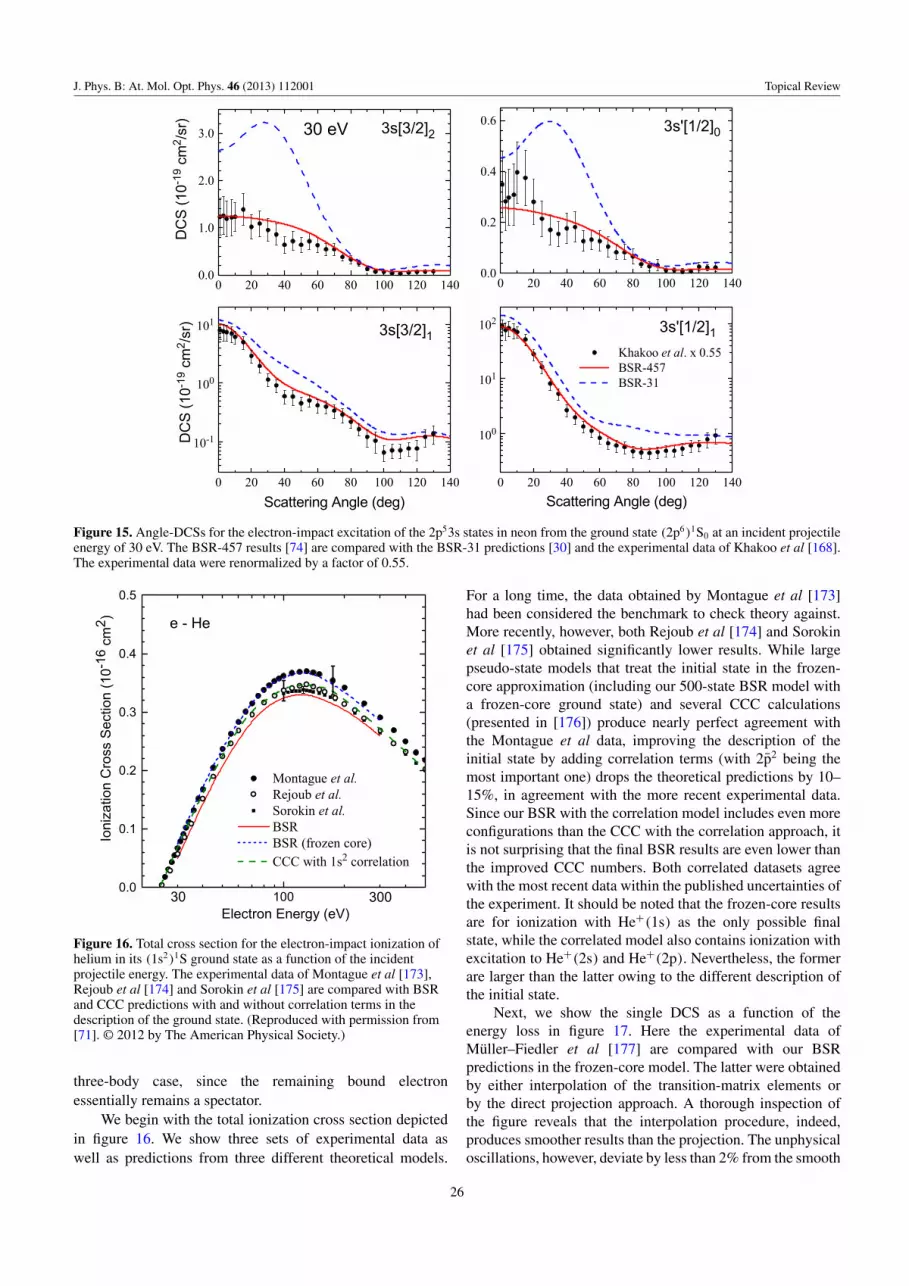
J. Phys. B: At. Mol. Opt. Phys. 46 (2013) 112001 Topical Review

Figure 15. Angle-DCSs for the electron-impact excitation of the 2p53s states in neon from the ground state (2p6)1S0 at an incident projectileenergy of 30 eV. The BSR-457 results [74] are compared with the BSR-31 predictions [30] and the experimental data of Khakoo et al [168].The experimental data were renormalized by a factor of 0.55.

Figure 16. Total cross section for the electron-impact ionization ofhelium in its (1s2)1S ground state as a function of the incidentprojectile energy. The experimental data of Montague et al [173],Rejoub et al [174] and Sorokin et al [175] are compared with BSRand CCC predictions with and without correlation terms in thedescription of the ground state. (Reproduced with permission from[71]. © 2012 by The American Physical Society.)

three-body case, since the remaining bound electronessentially remains a spectator.

We begin with the total ionization cross section depictedin figure 16. We show three sets of experimental data aswell as predictions from three different theoretical models.

For a long time, the data obtained by Montague et al [173]had been considered the benchmark to check theory against.More recently, however, both Rejoub et al [174] and Sorokinet al [175] obtained significantly lower results. While largepseudo-state models that treat the initial state in the frozen-core approximation (including our 500-state BSR model witha frozen-core ground state) and several CCC calculations(presented in [176]) produce nearly perfect agreement withthe Montague et al data, improving the description of theinitial state by adding correlation terms (with 2p2 being themost important one) drops the theoretical predictions by 10–15%, in agreement with the more recent experimental data.Since our BSR with the correlation model includes even moreconfigurations than the CCC with the correlation approach, itis not surprising that the final BSR results are even lower thanthe improved CCC numbers. Both correlated datasets agreewith the most recent data within the published uncertainties ofthe experiment. It should be noted that the frozen-core resultsare for ionization with He+(1s) as the only possible finalstate, while the correlated model also contains ionization withexcitation to He+(2s) and He+(2p). Nevertheless, the formerare larger than the latter owing to the different description ofthe initial state.

Next, we show the single DCS as a function of theenergy loss in figure 17. Here the experimental data ofMuller–Fiedler et al [177] are compared with our BSRpredictions in the frozen-core model. The latter were obtainedby either interpolation of the transition-matrix elements orby the direct projection approach. A thorough inspection ofthe figure reveals that the interpolation procedure, indeed,produces smoother results than the projection. The unphysicaloscillations, however, deviate by less than 2% from the smooth

26

J. Phys. B: At. Mol. Opt. Phys. 46 (2013) 112001 Topical Review

Figure 17. Single DCS for the electron-impact ionization of heliumin its (1s2)1S ground state for an incident projectile energy of100 eV. The experimental data of Muller–Fiedler et al [177](obtained by integrating their double-DCSs) are compared withBSR predictions (in the frozen-core model) generated byinterpolation and direct projection. (Reproduced with permissionfrom [71]. © 2012 by The American Physical Society.)

results and would not be detectable with current experimentaltechniques. As mentioned above, the projection approachis more generally applicable than the interpolation method.Hence, we use this example to illustrate the degree of validity.

The double-DCS as a function of the detection angle ofone of the outgoing electrons with fixed energy is depictedin figure 18. There is excellent agreement between our BSRresults and the experimental data of Muller–Fiedler et al [177]and also the CCC predictions [130]. For small energies ofthe detected electron (2 eV, 4 eV and 10 eV), the DDCSpeaks in the backward direction, while it is the other wayaround for large detection energies. This is consistent withthe expectation that the faster of the outgoing electron can beconsidered the ‘projectile’, which is not deflected very much.Consequently, the DDCS near the backward direction falls offfast with increasing detection angle of the faster of the twooutgoing electrons. This poses significant challenges to bothexperiment and theory, resulting in limited experimental dataand, particularly for 55 eV, in differences of up to a factorof 2 between the CCC and BSR predictions for large angles.Differences also occur for the case of near-symmetric energysharing between the two electrons (35 eV), but once again inan angular regime where there are no experimental data forcomparison. Finally, for a detection energy of 10 eV, the BSRpredictions agree better with experiment than those from theCCC calculation at angles less than 60◦, while it is the otherway around for angles above 120◦.

Figure 19 shows our results compared with the recentexperimental benchmark data of Ren et al [178] for electron-impact ionization of helium in its (1s2)1S ground withthe residual ion left in the He+(1s)2S state. The primaryenergy E0 is 70.6 eV and the two final-state electrons have

Figure 18. Double-DCS for the electron-impact ionization ofhelium in its (1s2)1S ground state for an incident projectile energyof 100 eV and a fixed energy of the detected electron as the functionof its detection angle. The experimental data of Muller–Fiedler et al[177] are compared with BSR and CCC [130] predictions.(Reproduced with permission from [71]. © 2012 by The AmericanPhysical Society.)

energies of 41.0 eV and 5.0 eV, respectively. These areexamples of asymmetric energy sharing between the twooutgoing electrons. The momentum vector of the incidentelectron and the faster outgoing electron with angle θ1 formthe scattering plane. Results are then presented for caseswhere the other electron with energy E2 is detected at avariable angle θ2 either in the same plane (the co-planararrangement) or in the ‘perpendicular plane’ that also containsthe incident momentum vector. Overall, we see excellentagreement with experiment as well as the CCC and TDCCpredictions presented by Ren et al [178]. Interestingly, thelargest differences between the theoretical predictions occurnear a detection angle of 180◦, where there are no experimentaldata available to decide between the three theories.

The next example is shown in figure 20, where wecompare the experimental data of Nixon et al [179] to our BSRresults. The data are for the doubly-symmetric perpendiculargeometry (see figure 1 of [179] for details), where themomentum vectors of both final-state electrons lie in the planeperpendicular to the incident beam direction, both outgoingelectrons have the same energy, and the angle between thetwo final-state momenta is varied. Since the experimental dataare relative and not cross-normalized either, we compare the

27

J. Phys. B: At. Mol. Opt. Phys. 46 (2013) 112001 Topical Review

Figure 19. TDCS for the electron-impact ionization of helium in its(1s2)1S ground with the residual ion left in the He+(1s)2S state. Theprimary energy E0 is 70.6 eV, and the final-state electrons haveenergies of 41.0 eV and 5.0 eV, respectively. The faster of the twoelectrons is detected at a fixed angle θ1 indicated for each panel,while the detection angle θ2 for the slower electron with energy E2 isvaried. The minus sign indicates the frequently used convention thatthe angles of the two electrons are counted clockwise for one andcounterclockwise for the other. The experimental data for theco-planar and perpendicular geometries, as well as the CCC andTDCC predictions, are from Ren et al [178].

relative angular dependence. Here we visually normalize theexperimental data to the absolute BSR numbers.

The overall agreement between experiment and the BSRresults is very good, certainly regarding the shape. However, asdiscussed by Bray et al [90], the situation regarding absolutenormalization is not so clear. The results for 180◦ in thisgeometry also appear in the coplanar geometry and hence,in principle, could be normalized to absolute data in thatplane. Only a few other theoretical predictions are available(CCC at 10 eV [133], both CCC and TDCC at 20 eV [180]).For 20 eV in particular, there is a significant difference inthe magnitudes predicted by CCC/TDCC and BSR, whilethe agreement between BSR and TDCC is better, though notperfect, for 10 eV. Clearly, both CCC and RMPS yield goodagreement with the measured angular dependence, while thecentre peak of the TDCC results for 20 eV seems too lowrelatively to the side peaks. We do not have an explanation forthe discrepancies in magnitude at the present time. We note,

Figure 20. TDCS for the electron-impact ionization of helium in its(1s2)1S ground with the residual ion left in the He+(1s)2S state. Theexperimental data of Nixon et al [179] for the doubly-symmetricperpendicular geometry are compared with the present BSRpredictions. Since the experimental data are relative and notcross-normalized, they were visually normalized to the BSR theory.Also available are CCC calculations for 10 eV [133] (long-dashedline), and both CCC and TDCC (short-dashed line) calculations for20 eV [180].

however, that the TDCS values are generally smaller at 20 eVcompared to 10 eV, and hence it is likely more difficult tocalculate them accurately at 20 eV.

The apparently largest discrepancy between experimentand theory at 35 eV, which is also seen in the shape, canbe attributed to the 2s2 and 2p2 doubly-excited autoionizingstates of helium near that energy (see, for example, deHaraket al [181]). The theoretical cross sections then become verysensitive to the electron energies chosen in the projection step,as well as to the quality of the description of the autoionizingstates.

As seen above, electron-impact ionization of He(1s2)1Sleaving the residual ion in the He+(1s)2S) ground state canalso be handled well by CCC, TDCC, and in many cases also byperturbative methods subject so some restrictions regarding the

28

J. Phys. B: At. Mol. Opt. Phys. 46 (2013) 112001 Topical Review

Figure 21. TDCS ratio for the electron-impact ionization of heliumin its (1s2)1S ground with the residual ion left in either theHe+(1s)2S state or the excited He+(n = 2) states. The primaryenergy E0 is either 112.6 eV (n = 1) or 153.4 eV (n = 2) and bothfinal-state electrons have energies of 44.0 eV. The experimental dataof Bellm et al [128] are compared with BSR results and predictionsfrom the hybrid DWB2-RMPS approach. (Reproduced withpermission from [70]. © 2011 by The American Physical Society.)

kinematics. The most significant progress achieved by the BSRwith pseudo-states method, therefore, was in the successfuldescription of a much more complex process, namely theionization of one 1s electron and simultaneous excitation ofthe other one [70]. This is a true, highly correlated four-bodyCoulomb process that posed major problems to theoreticalattempts for many years. The hybrid approach mentionedpreviously had been somewhat successful [126–128], butwas limited to highly asymmetric energy sharing and smallscattering angles of the projectile.

Figure 21 compares the BSR and DWB2-RMPSpredictions with the directly measured experimental cross-section ratios [128] for ionization without excitation (leavingthe electron in He+ in the 1s state) and ionization withexcitation to He+ (2s + 2p). The agreement between theBSR results and the experimental data is excellent at allangles of the reference electron between 24◦ and 56◦, and alldetection angles of the other electron between 25◦ and 115◦.As expected, the hybrid approach is inappropriate for largeangles of the fixed electron.

The study of more complex targets (e.g., neon, argon,etc) impose additional problems in the description of thetarget structure. While a few attempts have been made toapply the CCC and TDCC methods, once again in the single-active-electron approach, to other targets (e.g., [182, 183]),it is not clear how accurate the results might be in thelight of the necessary approximations made in the structuredescription. Until very recently, most theoretical work onsuch targets was still based on variants of the distorted-wave Born approximation (DWBA) pioneered by Madisonet al [184] and the previously mentioned first-order (DWB1-RM) [122] and later second-order (DWB2-RM) [123, 124]hybrid distorted-wave + R-matrix approach. Despite somesuccess, problems for the low-energy regime prevailed dueto a less than ideal (if any) description of the PCI between thetwo outgoing electrons. Attempts to fix this problem includethe use of asymptotically correct three-body wavefunctionsin the 3DW approach [185] or the ad hoc introduction ofsome version of the Gamov factor [186]. Serious problems,however, are the facts that the 3DW wavefunction may not besufficiently accurate at small distances between the projectileand the target (where the ionization occurs), while the Gamovfactor is known to be very problematic regarding the overallnormalization. Neither of these methods has been shown toyield a systematic and predictable improvement in the generalcase.

The first application of the BSR method to such systemswas carried out for the ionization of Ar(3p), where extensiveexperimental data were available for 200 eV [178] and 71 eV[187], respectively. While an unprecedented reproductionof the experimentally observed cross-section patterns as afunction of the emission angle for the slow electron at fixedelectron energies was observed, open questions remainedconcerning the dependence of the cross-section magnitude asa function of the projectile scattering angle. After a detailedanalysis of the BSR predictions as well as the DWB2-RM hybrid results [77], the data evaluation procedure onthe experimental side was revisited. It revealed that thisissue, to a large extent, can be assigned to a missing solid-angle correction factor in processing the experimental rawdata [188].

Very recently, the experiment was performed for theionization of Ne(2p) at an incident electron energy of100 eV [189], with particular emphasis on the proper cross-normalization of the results. The experimental side of this workwas carried out by employing an advanced reaction microscope[190, 191]). By means of homogeneous electric and magneticfields the residual ion and the two final-state electrons e1 and e2

are projected onto time- and position-sensitive detectors. Fromthe individually measured time-of-flight and position of eachparticle the three-dimensional momentum vector is calculated.Thus, full three-dimensional 3DCS are accessible. Since thecomplete experimentally accessible phase space is measuredsimultaneously, all relative 3DCS are cross normalized andonly a single global factor is required in comparison of theoryand experiment. This factor is used to put the 3DCS on anabsolute scale.

Figure 22 exhibits a three-dimensional 3DCS patternfor a projectile scattering angle of −10◦ and 8 eV (central)

29

J. Phys. B: At. Mol. Opt. Phys. 46 (2013) 112001 Topical Review

z

Ee0 = 100 eV ± 2.0 eV; θe1

= -10° ± 1.5°; Ee2 = 8 eV ± 2.0 eV

exp.

x

z

p0

qpe1

z

BSR

x

z

Figure 22. 3D triple-DCS for Ne(2p) ionization at an incident electron energy of 100 eV. The experimental pattern on the left is comparedwith the BSR predictions on the right. The scattering angle is θe1 = −10◦ ± 1.5◦, and the ejection energy is Ee2 = 8eV ± 2eV. (Reproducedwith permission from [189]. © 2013 by The American Physical Society.)

energy of the ejected electron. The left panel represents themeasured data while the BSR prediction is shown on the right.In this particular representation, the relative 3DCS is givenby the radial distance from the origin to the surface of theplot. The projectile with momentum p0 enters the interactionregion from below and after scattering has the momentumpe1

. The momentum transfer to the target system is indicatedby the arrow labelled q. Two general features are observable.Electrons emitted roughly in the direction of the momentumtransfer form the binary peak, while those emitted in theopposite direction form the recoil peak.

Here, the binary peak is split by a dip (in theory) in thedirection of q. This is the result of the characteristic momentumprofile of a p-orbital that has a node for vanishing momentum.Therefore, figure 22 exhibits a maximum cross section forelectron emission on a cone around the q direction. Due to thelow energy of the projectile, PCI is strong (as expected) and,consequently, the binary peak is suppressed near the forwarddirection. The qualitative comparison of experiment and theoryshows very good overall agreement, with the exception thatthe binary peak is no longer split in the experimental data (seefurther discussion below).

Furthermore, three planes are indicated in figure 22, whichwill be used to compare experiment and theory quantitativelyin figure 23. Those are the xz-plane or scattering plane (top),the yz-plane or perpendicular plane (centre) and the xy-planeor full-perpendicular plane (bottom). The global scaling factorused to normalize the experimental data to the BSR theorywas found by achieving the best fit to the binary peak in thescattering plane. It was subsequently applied to all other (48total) kinematics and planes [189], with overall impressiveagreement between experiment and the BSR predictions, notonly with regard to the angular dependence for each fixedset of final-state electron energies and detection angle of theprojectile, but also the cross-normalization.

Figure 23 shows results for the three planes for oneset of parameters, namely the incident electron energy of100 eV, the projectile detection angle of −10◦ and an ejectedelectron energy of 8 eV. We see excellent agreement betweenexperiment and the BSR predictions. For the coplanar case

(top panel), the DWB2-RM (which neglects PCI) shows a verypronounced split of the binary peak structure in the direction ofq. As seen already in figure 22, the peak towards smaller anglesstill exists in the BSR curve, but it is strongly suppressed by thePCI effects included in this model. The experimental data donot exhibit a small-angle peak at all, but it is not clear how muchweight can be put on the ‘shape-determining’ point at 25◦, i.e.,at the very edge of the data range. The DWB2-RM results arerelatively close to the BSR numbers, except for ejection angleswhere strong post-collision effects can be expected due to thetwo electrons leaving the target close to each other. This isnever the case for the full-perpendicular geometry, and henceDWB2-RM does best in this case (bottom panel of figure 23).

Finally, we can close the circle by showing how thesedetailed results can be useful for applications. Figure 24compares the total (elastic + excitation + ionization) crosssection for electron collisions with Ne atoms in their groundstate with a number of experimental data. We draw specialattention to the higher energies, where ionization processesbecome increasingly important. The figure also shows therelative importance of the contributions from individualcollision processes. Elastic scattering dominates over the entireenergy regime shown in the figure. Excitation processes, onthe other hand, only provide a relatively small contributionto the total cross section, while ionization becomes more andmore important with increasing projectile energy and makesup nearly 30% of the total cross section at 200 eV. The overallexcellent agreement with the available experimental dataconfirms the accuracy of the present approach. These results,including the important momentum-transfer cross sections, arenow available through the publicly accessible LXCat database[196].

3.2.5. Electron-impact coherence parameters, spin polariza-tions and spin asymmetries. As our final examples for elec-tron collisions, we show some recent BSR calculations tomodel experiments, in which the light emitted after electron-impact excitation is analysed or where the spin polarization ofthe electrons may play a role. We begin with a recent study

30

J. Phys. B: At. Mol. Opt. Phys. 46 (2013) 112001 Topical Review

0

0.2

0.4

0.6

0.8

0 60 120 180 240 300 360

TD

CS

(a.

u.)

θe2 (deg)

Ee1 = 100 eV ± 2 eV; θe1

= -10o ± 1.5o; Ee2 = 8 eV ± 2 eV

q

scattering plane

DWB2-RMBSR

0

0.2

0.4

0.6

0.8

0 60 120 180 240 300 360

TD

CS

(a.

u.)

θe2 (deg)

perpendicular plane

0

0.2

0.4

0.6

0.8

0 60 120 180 240 300 360

TD

CS

(a.

u.)

φe2 (deg)

full perpendicular plane

Figure 23. TDCS for the electron-impact ionization of Ne(2p) foran incident projectile energy of 100 eV, a scattering angle ofθe1 = −10◦ ± 1.5◦, and an ejection energy of Ee2 = 8 eV ± 2 eV forthe co-planar (top), perpendicular (centre) and full-perpendicular(bottom) planes. The experimental data of Pfluger et al [189] arecompared with predictions from the BSR model and DWB2-RMmodels.

[75], in which the light emitted after the excitation of Ne(2p53s)1P1 state by electron impact was observed in coinci-dence with the scattered projectile. The photon detector wasplaced perpendicular to the scattering plane and the polariza-tion of the light was analysed. Figure 25 exhibits the results forthe circular polarization P3. This is a particularly interestingparameter that has drawn much attention over the years dueto a propensity rule that predicts P3 to start off with negativevalues at small scattering angles. This corresponds to a posi-tive angular momentum transfer, which one would intuitivelyexpect from a classical picture. A detailed discussion can befound, for example, in the book by Andersen and Bartschat[197].

The top part of figure 25 shows how the BSR predictionsconverge with the number of states in the close-coupling

Figure 24. Total cross section for electron scattering from neon. TheBSR-679 predictions [73] for elastic scattering alone, elasticscattering plus excitation, and Wagenaar and de Heer [192], Gulleyet al [193], Szmytkowski et al [194] and Baek and Grosswendt[195].

-0.4

-0.2

0.0

0.2

0.4Ne 1P1; 25 eV

P3

(a)

5-st15-st46-st

457-st

-0.8

-0.6

-0.4

-0.2

0.0

0.2

0 10 20 30 40 50scattering angle (deg)

P3

Ne 1P1; 25 eVAr 1P1; 20 eVKr 1P1; 20 eVXe 1P1; 15 eV

Figure 25. Top: circular light polarization P3 for the Ne (2p53s)1P1

state, as predicted by the BSR model with different numbers ofcoupled states. Bottom: circular light polarization P3 for thecorresponding lowest 1P1 states in Ne, Ar, Kr and Xe, as predictedby BSR calculations with a sufficient number of states forconvergence. (Reproduced with permission from [75]. © 2012 byThe American Physical Society.)

expansion. A simple five-state model is completely inadequatefor this case, while the apparently converged 457-state model,including a large number of pseudo-states, provides excellentagreement with the experimental data. Interestingly, the

31

J. Phys. B: At. Mol. Opt. Phys. 46 (2013) 112001 Topical Review

0.2

0.3

0.4

0.5

0.6

0.7

0.8

8 9 10 11 12 13 14 15 16 17 18

P1

-0.2

-0.1

0

0.1

0.2

8 9 10 11 12 13 14 15 16 17 18

P2

-0.2

-0.1

0

0.1

0.2

8 9 10 11 12 13 14 15 16 17 18

Energy (eV)

P3

Figure 26. P1, P2 and P3 for the 185 nm line in mercury for incidentenergies between 8 and 18 eV. Solid circles: experimental results;solid line: DBSR-36 calculation. Since P2 and P3 are proportional tothe electron polarization (P1 does not depend on it), their values arenormalized to 100% electron polarization. (Reproduced withpermission from [66]. © 2009 by The American Physical Society.)

violation of the propensity rule seems to be limited to a smallenergy range around 25 eV and also to the Ne target. Asseen in the bottom panel of figure 25, the other noble gases arebehaving ‘normal’. It is worth mentioning that the unusual, butthen confirmed, BSR predictions triggered the experimentalinvestigation in this case, with further work currently being inprogress.

Figure 26 shows results for the angle-integrated lightpolarizations P1, P2 and P3 for electron-impact excitation of theHg(6s6p)1P1 state in the incident-energy range from 8 to 18 eV[66]. In this case the scattered electrons were not observed,but the incident electrons are transversely spin-polarized. Thetwo linear polarizations P1(0◦, 90◦) and P2(45◦, 135◦) aredefined with linear polarization filters set at the angles givenin parentheses relative to the incident beam direction, whilethe photon detector is aligned parallel to the initial spin-

polarization vector. The energy range shown here is verychallenging, both experimentally and theoretically, due toa wealth of resonances above the first ionization thresholdof 10.4 eV in Hg, the vacuum ultraviolet nature of theemitted radiation and the relatively small values of P2 andP3. Not surprisingly, not all details of the structure couldbe mapped one-to-one between experiment and the 36-statefully relativistic DBSR theory (DBSR-36), but the overallagreement is very satisfactory.

Another observable that is often studied when spin-polarized electrons are available is the spin-asymmetryfunction SA, which determines a left–right asymmetry in theDCS when the incident electron beam is spin-polarized with apolarization vector perpendicular to the scattering plane [198].Many experiments for a variety of targets were performed overthe years in Munster in the groups of Kessler and Hanne, and aparticularly challenging case is the lead atom. With a nuclearcharge of Z = 82, it should be described in a fully relativisticframework, and the four electrons in the 6s and 6p sub-shellsstrongly interact with each other. While some theories wereable to describe elastic scattering in a reasonable way, theywere either inapplicable or simply inadequate for inelastictransitions.

Figure 27 shows the spin-asymmetry function SA afterthe electron-impact excitation of the (6p2)3P0 → (6p2)3P2

transition in Pb. We see a dramatic improvement in theagreement between the experimental data over Geesmannet al [199] achieved by two different fully-relativistic DBSRmodels [69] with 20 (DBSR-20) and 31 (DBSR-31) states,respectively, compared to a five-state semirelativistic BPcalculation (BPRM-5) [200] performed at the time of theexperiment over 20 years ago. It is truly remarkable that it hastaken this long for theory to catch up with these benchmarkexperiments.

3.3. Photoionization and photodetachment

As mentioned above, the BSR method can also be usedto calculate photo-induced processes. Except for a slightchange in the boundary conditions (see the theory section), theproblem effectively reduces to calculating the relevant dipolematrix elements between the initial bound state and the finalcontinuum state involving the scattering of the ejected electronfrom the residual ion in photoionization or the neutral atomin photodetachment. Not surprisingly, the BSR approach withnonorthogonal orbitals can provide accurate descriptions of allthe necessary ingredients.

3.3.1. Weak-field steady-state radiation. Figures 28 and 29exhibit BSR results for the photoionization of potassium fromits 4s ground state or the 4p excited state as a function of thephotoelectron energy. For the ground state, there is excellentagreement between the results obtained in the length andvelocity forms of the dipole operator, respectively, as wellas with the experimental data of Marr and Creek [202]. Thecalculations [82] clearly favour the latter datasets over theformer measurements performed by Hudson and Carter [203].A number of other calculations were carried out for thisproblem as well. Details can be found in [82].

32

J. Phys. B: At. Mol. Opt. Phys. 46 (2013) 112001 Topical Review

-1.0

-0.5

0.0

0.5

0 20 40 60 80 100 120 140

SA

2.5 eV3P0 - 3P2

DBSR-20DBSR-31

-1.0

-0.5

0.0

0.5

0 20 40 60 80 100 120 140

SA

2.5 eV3P0 - 3P2

-1.0

-0.5

0.0

0.5

0 20 40 60 80 100 120 140

SA

2.5 eV3P0 - 3P2

-1.0

-0.5

0.0

0.5

0 20 40 60 80 100 120 140

SA

2.5 eV3P0 - 3P2

-1.0

-0.5

0.0

0.5

0 20 40 60 80 100 120 140

3 eV

-1.0

-0.5

0.0

0.5

0 20 40 60 80 100 120 140

3 eV

-1.0

-0.5

0.0

0.5

0 20 40 60 80 100 120 140

3 eV

-1.0

-0.5

0.0

0.5

0 20 40 60 80 100 120 140

3 eV

BPRM-5

-0.5

0.0

0.5

0 20 40 60 80 100 120 140

SA

4 eV

-0.5

0.0

0.5

0 20 40 60 80 100 120 140

SA

4 eV

-0.5

0.0

0.5

0 20 40 60 80 100 120 140

SA

4 eV

-0.5

0.0

0.5

0 20 40 60 80 100 120 140

SA

4 eV

-0.4

-0.2

0.0

0.2

0.4

0.6

0 20 40 60 80 100 120 140

5 eV

-0.4

-0.2

0.0

0.2

0.4

0.6

0 20 40 60 80 100 120 140

5 eV

-0.4

-0.2

0.0

0.2

0.4

0.6

0 20 40 60 80 100 120 140

5 eV

-0.4

-0.2

0.0

0.2

0.4

0.6

0 20 40 60 80 100 120 140

5 eV

-0.2

0.0

0.2

0.4

0.6

0 20 40 60 80 100 120 140

SA

6 eV

-0.2

0.0

0.2

0.4

0.6

0 20 40 60 80 100 120 140

SA

6 eV

-0.2

0.0

0.2

0.4

0.6

0 20 40 60 80 100 120 140

SA

6 eV

-0.2

0.0

0.2

0.4

0.6

0 20 40 60 80 100 120 140

SA

6 eV

-0.2

0.0

0.2

0.4

0 20 40 60 80 100 120 140

9 eV

-0.2

0.0

0.2

0.4

0 20 40 60 80 100 120 140

9 eV

-0.2

0.0

0.2

0.4

0 20 40 60 80 100 120 140

9 eV

0.0

0.1

0.2

0.3

0 20 40 60 80 100 120 140

SA

Scattering Angle (deg)

11 eV

0.0

0.1

0.2

0.3

0 20 40 60 80 100 120 140

SA

Scattering Angle (deg)

11 eV

0.0

0.1

0.2

0.3

0 20 40 60 80 100 120 140

SA

Scattering Angle (deg)

11 eV

0.0

0.1

0.2

0.3

0 20 40 60 80 100 120 140

SA

Scattering Angle (deg)

11 eV

-0.2

0.0

0.2

0 20 40 60 80 100 120 140

Scattering Angle (deg)

14 eV

-0.2

0.0

0.2

0 20 40 60 80 100 120 140

Scattering Angle (deg)

14 eV

-0.2

0.0

0.2

0 20 40 60 80 100 120 140

Scattering Angle (deg)

14 eV

-0.2

0.0

0.2

0 20 40 60 80 100 120 140

Scattering Angle (deg)

14 eV

RDW

Figure 27. Spin-asymmetry function SA for the electron-impact excitation of the (6p2)3P0 → (6p2)3P2 transition in Pb for a variety ofprojectile energies. The DBSR-20 and DBSR-31 predictions [69] are compared with the experimental data of Geesmann et al [199]. Whereavailable, we also show BPRM-5 [200] and RDW [201] results.

The photodetachment cross section of He− from themetastable (1s2s2p)4Po state is depicted in figure 30. Thisis one of the earlier applications of the BSR approach to arelatively simple problem, which can also be solved reliablyusing other approaches [206, 207]. Hence, it is not surprisingthat three different sets of theoretical predictions agree wellwith each other across the first maximum around a photonenergy of 39 eV. A discussion about the potential reasonsfor the discrepancies between experiment and theory in thisregime can be found in [78]. In the high-energy regime, on theother hand, the agreement between the experimental data andthe BSR results is excellent.

3.3.2. Strong-field short-pulse radiation. As our firstexample from this area, figure 31 shows the response of the Neatom to pulses with central photon energies of 11.6 and 7.3 eV,respectively. In these cases, at least two or three photons, needto be absorbed in order to ionize the system. This was ourfirst attempt at such a problem, and hence we only used the

ground state (1s22s22p5)2P of Ne+ as the target state for the‘half collision’ of the ejected electron with the residual ion.In order to ensure converged results for the above cases, wecoupled LS symmetries up to a total orbital angular momentumLmax = 6 for the electron−ion collision system. Note thatexcitation rather than ionization appears as the dominatingreaction process for ω = 0.27 au and the laser parameterschosen here.

For the argon target, we performed a more sophisticatedcalculation [86], in which we coupled three states of the Ar+

ion. In this project, we studied the effects of the finite pulselength and the intensity on various intermediate resonancestates. Figure 32 depicts the excitation probability at differentphoton energies. Rabi oscillations occur when the photonenergy matches the energy gap between the ground state and,in this case, the (3p54s)1P excited state. This matching leads tooscillations in the excitation probability with a large amplitudeand a long period. There are still oscillations when the photonenergy is tuned away from the energy gap, but they have muchsmaller amplitudes and shorter periods.

33

J. Phys. B: At. Mol. Opt. Phys. 46 (2013) 112001 Topical Review

Figure 28. Photoionization cross sections for the 4s ground state ofpotassium as a function of photoelectron energy. The solid anddotted lines represent the length and velocity BSR results,respectively [82]. The experimental data are from Marr and Creek[202] (solid circles) and from Hudson and Carter [203] (solidtriangles).

Figure 29. Photoionization cross sections for the 4p3/2 and 4p1/2

excited levels of potassium as a function of the photoelectron energy.The solid and dashed lines represent the BSR results (length form)for the 4p3/2 and 4p1/2levels, respectively [82]. The experimentaldata are from Petrov et al [204] (solid circles) without resolvedfinestructure and from Amin et al [205] for the 4p3/2 (inverted solidtriangles) and 4p1/2 (upward solid triangles) initial states.

As a result of coupling several ionic states, Rydberg-type resonances converging to different thresholds can beobserved. However, both the finite length of the pulse andits intensity have an effect on the details of the observedstructures. Figure 33 shows the effect of the laser intensityon the generalized two-photon cross section. While both peakintensities, 1012 and 1013 W cm−2, still lie in the perturbativeregime, the height of the first resonance peak is significantlydiminished for the more intense laser field. Similar results havebeen obtained by another time-dependent R-matrix approach,which is independently being developed by the Belfast group[139].

Figure 34 exhibits two examples for the single ionizationrates in argon [86] obtained in few-cycle laser pulses of

(a)

(b)

Figure 30. Total photodetachment cross section for He− in themetastable (1s2s2p)4Po state as a function of the photon energy[78]. The BSR results (solid line) are compared with theexperimental data of Berrah et al [208] and near the first maximumwith predictions from a standard R-matrix calculation [206] and acomplex-rotation CI calculation [207]. (b) Comparison between theBSR predictions (convoluted with a 70 meV FWHM Gaussian) andhigh-resolution experimental data in the higher energy regime.

different lengths, intensities and central wavelengths. Thereis clearly a nontrivial dependence on the various laserparameters, and once again resonances appear when the photonwavelength is varied. These predictions are currently awaitingexperimental tests, but they show the richness of effectsthat can be expected in complex targets where inter-shellcorrelation effects play an important role.

As our final example, we consider the two-photon DI ofthe helium atom by the absorption of two photons at differentcentral photon energies. In other words, the target heliumatom is exposed to the irradiation by two laser pulses, ofpotentially different frequencies and with a controllable timedelay. Specifically, the following two-colour laser parameterswere used for the results shown in figure 35: pulse 1 hasa central photon energy of 35.3 eV and a peak intensity of1014 W cm−2, while the corresponding parameters for pulse2 are 57.1 eV and 1013 W cm−2, respectively. The length ofeach pulse is 10 optical cycles with a Gaussian envelope,thus corresponding to pulse lengths of about 1.2 and 0.7fs, respectively. We are interested in the mechanism for theejection of two electrons when the time delay between thetwo pulses is varied. We define this delay as the time distance

34

J. Phys. B: At. Mol. Opt. Phys. 46 (2013) 112001 Topical Review

excitationionization

survival

ω = 0.425 a.u.

Time (optical cycles)

Exc

itat

ion/i

oniz

atio

npro

bab

ility

Surv

ival

pro

bab

ility

0.07

0.06

0.05

0.04

0.03

0.02

0.01

0.00109876543210

1.00

0.98

0.96

0.94

0.92

excitationionization

survival

ω = 0.27 a.u.

Time (optical cycles)

Exc

itat

ion/i

oniz

atio

npro

bab

ility

Surv

ival

pro

bab

ility

0.05

0.04

0.03

0.02

0.01

0.00109876543210

1.00

0.98

0.96

0.94

0.92

Figure 31. Ground-state survival (left scale) and total excitation andionization probabilities (right scale) for Ne exposed to 10-cyclelaser pulses of peak intensity 3.5 × 1014 W cm−2 with a Gaussianenvelope. The central laser frequencies are 0.425 au (11.6 eV, toppanel) and 0.27 au (7.3 eV, bottom panel).

ω = 13 eVω = 12 eVω = 11 eV (×10)ω = 10 eV (×50)

Time (optical cycles)

Exc

itat

ion

pro

bab

ility

302520151050

1.0

0.8

0.6

0.4

0.2

0.0

Figure 32. Excitation probability of argon for a 30-cycle laser pulsewith the peak intensity of 2 × 1013 W cm−2 and photon energies of10, 11, 12 and 13 eV. Note the different scales for the individualphoton energies.

between the peak intensities. Consequently, there is no overlapat all between the two pulses for a delay of about 0.95 fs,corresponding to a little less than 40 au of time (1 au ≈ 24attoseconds).

Figure 35 shows the results for a variety of delays, rangingfrom about −120 (i.e., the second photon with the higherenergy comes first) to 600 attoseconds. Not surprisingly, theprobability for DI is small in the first case, since the onlychance for this process to happen is the two photons working

I0 = 1013 W/cm2I0 = 1012 W/cm2R-matrix Floquet

(3s3p63d) 1D /(5s) 1S

(3s3p64s) 1S

(3p54s) 1Po

Photon energy (eV)

Gen

eral

ized

cros

sse

ctio

n(c

m4s)

15141312111098

10−48

10−49

10−50

Figure 33. Effect of the laser peak intensity on the generalizedtwo-photon cross section for a 30-cycle laser pulse interacting withargon. The Floquet-results are from McKenna and van der Hart[209].

τ = 10 o.c.τ = 30 o.c.

I0 = 1013 W/cm2

Photon energy (eV)

Ioniz

atio

nyi

eld

15141312111098765

10−1

10−2

10−3

10−4

10−5

I0 = 1014 W/cm2I0 = 1013 W/cm2τ = 10 o.c.

Photon energy (eV)

Ioniz

atio

nyi

eld

15141312111098765

100

10−1

10−2

10−3

10−4

10−5

Figure 34. Ionization yield as a function of photon energy in10-cyle and 30-cycle laser pulses of peak intensity 1013 W cm−2

(top) and for 10-cycle laser pulses with peak intensities of 1013 and1014 W cm−2 (bottom).

together on the two electrons. Even when the two pulses comesimultaneously, the probability for double ejection remainsrelatively small, and the peak for equal-energy sharing is aclear indication of the direct process. With increasing timedelay, the peaks expected for the sequential process—one at

35

J. Phys. B: At. Mol. Opt. Phys. 46 (2013) 112001 Topical Review

Figure 35. Energy distributions of the two escaping electrons in two-colour laser pulses of ten optical cycles each. The laser parameters are:ω1 = 35.3 eV at a peak intensity of 1014 W cm−2 and ω2 = 57.1 eV at a peak intensity of 1013 W cm−2. The delay between the two pulses isvaried between −121 as and +605 as. See text for details.

10.7 eV and the other at 2.7 eV, corresponding to the 35.1 eVphoton ionizing the neutral helium atom with an ionizationpotential of 24.6 eV and the other one ionizing the He+(1s)ion with an ionization potential of 54.4 eV—start to grow, butthe two processes still have about equal weight for a time delayas large as 400 attoseconds.

From this example, it is clear that the time delay plays adecisive role in determining how the two electrons are ejectedby two-colour XUV laser pulses. Depending on the detailsof the time delay, the electrons can be ejected in ways eithersimilar to the sequential or the nonsequential process. Ourfindings qualitatively agree with those of Foumouo et al [210]for the two-colour problem and Feist et al [211] in the single-colour problem. They serve as an independent confirmation oftheir predictions, and also give us confidence in our computercode.

4. Conclusions and outlook

We have presented the general ideas behind the B-splineR-matrix (BSR) approach with nonorthogonal orbitals anda variety of examples for applications of the method toproblems in atomic structure, electron collisions and photon-driven processes. Allowing for nonorthogonal one-electronorbitals and hence eliminating orthogonality restrictions thatare introduced in many other theoretical formulations merelyfor computational convenience, rather than physical necessity,often increases the accuracy that can be obtained in the targetdescription while a subsequent collision calculation is still

possible. From a numerical point of view, key ingredients ofthe method are the B-splines that represent the orbitals of theactive target electrons as well as the projectile, if necessary.

We presently have a suite of semirelativistic computercodes based on [1] that has been fully parallelized to runefficiently on large clusters such as Lonestar [212], Stampede[213] and Gordon [214]. As summarized in tables 1−4,results from this program, and its fully relativistic (DBSR)companion, have been used both to study fundamentalphysics and to generate a variety of atomic data for plasmaapplications. We are currently working on parallelizing theDBSR suite of codes. We also plan to further extend thecapabilities of handling time-dependent processes, and wehope to move towards simple diatomic molecules in theforeseeable future.

Acknowledgments

Many colleagues have contributed to this work. There aretoo many to mention explicitly, but their names appear inthe reference list of our many joint publications. We would,however, like to thank Professor Dmitry Fursa for detailedand constructive comments that have improved the manuscriptsubstantially. Over the past ten years, this work has beensupported by the United States National Science Foundationunder grants no. PHY-0244470, no. PHY-0311161, no.PHY-0555226, no. PHY-0757755, no. PHY-0903818, no.PHY-1068140, and no. PHY-1212450 and by the TeraGrid/XSEDE allocation no. TG-PHY-090031.

36

J. Phys. B: At. Mol. Opt. Phys. 46 (2013) 112001 Topical Review

References

[1] Zatsarinny O 2006 Comput. Phys. Commun. 174 273–356[2] Zatsarinny O and Fischer C F 2009 Comput. Phys. Commun.

180 2041–65[3] Fischer C F and Zatsarinny O 2009 Comput. Phys. Commun.

180 879–86[4] Zatsarinny O and Fischer C 2000 Comput. Phys. Commun.

124 247–89[5] Guan X, Noble C J, Zatsarinny O, Bartschat K

and Schneider B I 2009 Comput. Phys. Commun.180 2401–9

[6] Zatsarinny O and Fischer C 2002 J. Phys. B: At. Mol. Opt.Phys. 35 4669–83

[7] Zatsarinny O and Bartschat K 2009 Phys. Scr. T 134 014020[8] Zatsarinny O and Bartschat K 2006 J. Phys. B: At. Mol. Opt.

Phys. 39 2861–75[9] Tayal S S and Zatsarinny O 2010 Astrophys. J. Suppl. Ser.

188 32–45[10] Zatsarinny O and Bartschat K 2006 J. Phys. B: At. Mol. Opt.

Phys. 39 2145–58[11] Dasgupta A, Apruzese J P, Zatsarinny O, Bartschat K

and Fischer C F 2006 Phys. Rev. A 74 012509[12] Zatsarinny O, Bartschat K, Mitroy J and Zhang J Y 2009

J. Chem. Phys. 130 124310[13] Zatsarinny O, Bartschat K, Zhang J Y and Mitroy J 2009

Mol. Phys. 107 2387–93[14] Zatsarinny O and Bartschat K 2005 Phys. Rev. A 72 020702[15] Tayal S S and Zatsarinny O 2011 Astrophys. J. 743 206[16] Tayal S S and Zatsarinny O 2010 Astron. Astrophys. 510 A79[17] Tayal S S and Zatsarinny O 2008 Phys. Rev. A 78 012713[18] Ward R, Cubric D, Bowring N, King G C, Read F H,

Fursa D V, Bray I, Zatsarinny O and Bartschat K 2011J. Phys. B: At. Mol. Opt. Phys. 44 045209

[19] Lange M, Matsumoto J, Lower J, Buckman S, Zatsarinny O,Bartschat K, Bray I and Fursa D 2006 J. Phys. B: At. Mol.Opt. Phys. 39 4179–90

[20] Stepanovic M, Minic M, Cvejanovic D, Jureta J, Kurepa J,Cvejanovic S, Zatsarinny O and Bartschat K 2006 J. Phys.B: At. Mol. Opt. Phys. 39 1547–61

[21] Zatsarinny O, Bartschat K, Bandurina L and Gedeon V 2005Phys. Rev. A 71 042702

[22] Tayal S and Zatsarinny O 2005 J. Phys. B: At. Mol. Opt.Phys. 38 3631–45

[23] Zatsarinny O and Tayal S 2003 Astrophys. J. Suppl. Ser.148 575–82

[24] Zatsarinny O and Tayal S 2002 J. Phys. B: At. Mol. Opt.Phys. 35 241–53

[25] Zatsarinny O and Tayal S 2001 J. Phys. B: At. Mol. Opt.Phys. 34 1299–319

[26] Zatsarinny O, Bartschat K and Tayal S 2006 J. Phys. B: At.Mol. Opt. Phys. 39 1237–49

[27] Zatsarinny O and Tayal S 2002 J. Phys. B: At. Mol. Opt.Phys. 35 2493–503

[28] Zatsarinny O and Tayal S 2001 J. Phys. B: At. Mol. Opt.Phys. 34 3383–400

[29] Wang Y, Zatsarinny O, Bartschat K and Booth J P 2013Phys. Rev. A 87 022703

[30] Zatsarinny O and Bartschat K 2004 J. Phys. B: At. Mol. Opt.Phys. 37 2173–89

[31] Allan M, Franz K, Hotop H, Zatsarinny O and Bartschat K2009 J. Phys. B: At. Mol. Opt. Phys. 42 044009

[32] Allan M, Franz K, Hotop H, Zatsarinny O and Bartschat K2006 J. Phys. B: At. Mol. Opt. Phys. 39 L139–44

[33] Bommels J, Franz K, Hoffmann T, Gopalan A, Zatsarinny O,Bartschat K, Ruf M and Hotop H 2005 Phys. Rev. A71 012704

[34] Dodt D, Dinklage A, Fischer R, Bartschat K, Zatsarinny Oand Loffhagen D 2008 J. Phys. D: Appl. Phys. 41 205207

[35] Dodt D, Dinklage A, Bartschat K and Zatsarinny O 2010New J. Phys. 12 073018

[36] Borovik A, Zatsarinny O and Bartschat K 2008 J. Phys. B:At. Mol. Opt. Phys. 41 035206

[37] Bartschat K, Zatsarinny O, Bray I, Fursa D and Stelbovics A2004 J. Phys. B: At. Mol. Opt. Phys. 37 2617–39

[38] Zatsarinny O, Bartschat K, Gedeon S, Gedeon V, Lazur Vand Nagy E 2009 Phys. Rev. A 79 052709

[39] Gedeon V, Gedeon S, Lazur V, Nagy E, Zatsarinny Oand Bartschat K 2012 Phys. Rev. A 85 022711

[40] Zatsarinny O and Bartschat K 2004 J. Phys. B: At. Mol. Opt.Phys. 37 4693–706

[41] Allan M, Zatsarinny O and Bartschat K 2006 Phys. Rev. A74 030701

[42] Khakoo M A, Zatsarinny O and Bartschat K 2011 J. Phys. B:At. Mol. Opt. Phys. 44 169801

[43] Khakoo M A, Zatsarinny O and Bartschat K 2011 J. Phys. B:At. Mol. Opt. Phys. 44 015201

[44] Bartschat K and Zatsarinny O 2007 J. Phys. B: At. Mol. Opt.Phys. 40 F43–9

[45] Borovik A, Grum-Grzhimailo A, Bartschat Kand Zatsarinny O 2005 J. Phys. B: At. Mol. Opt. Phys.38 1081–92

[46] Borovik A A Jr, Borovik A A, Zatsarinny O and Bartschat K2006 Phys. Rev. A 73 062701

[47] Zatsarinny O, Bartschat K, Bandurina L and Gedeon S 2007J. Phys. B: At. Mol. Opt. Phys. 40 4023–31

[48] Zatsarinny O, Bartschat K, Gedeon S, Gedeon V and Lazur V2006 Phys. Rev. A 74 052708

[49] Zatsarinny O, Bartschat K, Suvorov V, Teubner P J Oand Brunger M J 2010 Phys. Rev. A 81 062705

[50] Zatsarinny O and Bartschat K 2010 Phys. Rev. A 82 062703[51] Zatsarinny O and Bartschat K 2005 Phys. Rev. A 71 022716[52] Napier S A, Cvejanovic D, Williams J F, Pravica L, Fursa D,

Bray I, Zatsarinny O and Bartschat K 2009 Phys. Rev. A79 042702

[53] Pravica L, Williams J F, Cvejanovic D, Samarin S,Bartschat K, Zatsarinny O, Stauffer A D and Srivastava R2011 Phys. Rev. A 83 040701

[54] Zatsarinny O et al 2011 Phys. Rev. A 83 042702[55] Hoffmann T H, Ruf M W, Hotop H, Zatsarinny O,

Bartschat K and Allan M 2010 J. Phys. B: At. Mol. Opt.Phys. 43 085206

[56] Allan M, Zatsarinny O and Bartschat K 2011 J. Phys. B: At.Mol. Opt. Phys. 44 065201

[57] Zatsarinny O, Bartschat K and Allan M 2011 Phys. Rev. A83 032713

[58] Borovik A, Roman V, Zatsarinny O and Bartschat K 2013J. Phys. B: At. Mol. Opt. Phys. 46 015203

[59] Dressler R A, Chiu Y H, Zatsarinny O, Bartschat K,Srivastava R and Sharma L 2009 J. Phys. D: Appl. Phys.42 185203

[60] Borovik A, Kupliauskiene A and Zatsarinny O 2011 J. Phys.B: At. Mol. Opt. Phys. 44 145203

[61] Zatsarinny O and Bartschat K 2010 J. Phys. B: At. Mol. Opt.Phys. 43 074031

[62] Zatsarinny O and Bartschat K 2008 Phys. Rev. A 77 062701[63] Zatsarinny O, Bartschat K, Maslov M, Brunger M J

and Teubner P J O 2008 Phys. Rev. A 78 042713[64] Maslov M, Brunger M J, Teubner P J O, Zatsarinny O,

Bartschat K, Fursa D, Bray I and McEachran R P 2008Phys. Rev. A 77 062711

[65] Zatsarinny O and Bartschat K 2009 Phys. Rev. A 79 042713[66] Juttemann F, Hanne G F, Zatsarinny O and Bartschat K 2009

Phys. Rev. A 79 042712[67] Juttemann F, Hanne G F, Zatsarinny O, Bartschat K,

Srivastava R, Gangwar R K and Stauffer A D 2010 Phys.Rev. A 81 012705

37

J. Phys. B: At. Mol. Opt. Phys. 46 (2013) 112001 Topical Review

[68] Hamelbeck V, Hanne G F, Zatsarinny O, Bartschat K,Gangwar R K and Srivastava R 2009 Phys. Rev. A80 062711

[69] Zatsarinny O, Wang Y and Bartschat K 2013 J. Phys. B: At.Mol. Opt. Phys. 46 035202

[70] Zatsarinny O and Bartschat K 2011 Phys. Rev. Lett.107 023203

[71] Zatsarinny O and Bartschat K 2012 Phys. Rev. A 85 062709[72] Wang Y, Zatsarinny O and Bartschat K 2013 Phys. Rev. A

87 012704[73] Zatsarinny O and Bartschat K 2012 Phys. Rev. A 85 062710[74] Zatsarinny O and Bartschat K 2012 Phys. Rev. A 86 022717[75] Hargreaves L R, Campbell C, Khakoo M A, Zatsarinny O

and Bartschat K 2012 Phys. Rev. A 85 050701[76] Ren X, Pfluger T, Ullrich J, Zatsarinny O, Bartschat K,

Madison D H and Dorn A 2012 Phys. Rev. A 85 032702[77] Zatsarinny O and Bartschat K 2012 Phys. Rev. A 85 032708[78] Zatsarinny O, Gorczyca T and Fischer C 2002 J. Phys. B: At.

Mol. Opt. Phys. 35 4161–78[79] Gorczyca T, Zatsarinny O, Zhou H, Manson S, Felfli Z

and Msezane A 2003 Phys. Rev. A 68 050703[80] Berrah N, Bilodeau R C, Dumitriu I, Bozek J D, Gibson N D,

Walter C W, Ackerman G D, Zatsarinny Oand Gorczyca T W 2007 Phys. Rev. A 76 032713

[81] Zatsarinny O and Bartschat K 2006 Phys. Rev. A 73 022714[82] Zatsarinny O and Tayal S S 2010 Phys. Rev. A 81 043423[83] Fischer C F and Zatsarinny O 2007 Theor. Chem. Acc.

118 623–30[84] Guan X, Zatsarinny O, Noble C J, Bartschat K

and Schneider B I 2009 J. Phys. B: At. Mol. Opt. Phys.42 134015

[85] Guan X, Zatsarinny O, Bartschat K, Schneider B I, Feist Jand Noble C J 2007 Phys. Rev. A 76 053411

[86] Guan X, Noble C J, Zatsarinny O, Bartschat Kand Schneider B I 2008 Phys. Rev. A 78 053402

[87] Bachau H, Cormier E, Decleva P, Hansen J E and Martin F2001 Rep. Prog. Phys. 64 1815

[88] de Boor C 1978 A Practical Guide to Splines (New York:Springer)

[89] Bray I, Fursa D V, Kheifets A S and Stelbovics A T 2002J. Phys. B: At. Mol. Opt. Phys. 35 R117

[90] Bray I, Fursa D, Kadyrov A, Stelbovics A, Kheifets Aand Mukhamedzhanov A 2012 Phys. Rep. 520 135–74

[91] Burke P G and Robb W R 1975 Adv. At. Mol. Phys. 11 143[92] Burke P G and Berrington K A 1993 Atomic and Molecular

Processes: an R-Matrix Approach (Bristol: Institute ofPhysics Publishing)

[93] Burke P G 2011 R-Matrix Theory of Atomic Collisions (NewYork: Springer)

[94] Berrington K A, Eissner W and Norrington P H 1995Comput. Phys. Commun. 92 290

[95] Sunderland A, Noble C, Burke V and Burke P 2002 Comput.Phys. Commun. 143 311

[96] Badnell N R 2012 http://amdpp.phyd.strath.ac.uk/rmatrix[97] Burke P G, Noble C J and Scott M P 1987 Proc. R. Soc. A

410 911[98] Fano U and Lee C M 1973 Phys. Rev. Lett. 31 15[99] Plummer M and Noble C 1999 J. Phys. B: At. Mol. Opt.

Phys. 32 L345[100] Bartschat K, Hudson E, Scott M, Burke P and Burke V 1996

J. Phys. B: At. Mol. Opt. Phys. 29 115–23[101] Gorczyca T and Badnell N 1997 J. Phys. B: At. Mol. Opt.

Phys. 30 3897[102] Gorczyca T W, Robicheaux F, Pindzola M S, Griffin D C

and Badnell N 1995 Phys. Rev. A 52 3877[103] Bartschat K 1998 Comput. Phys. Commun. 114 168[104] van der Hart H W 1997 J. Phys. B: At. Mol. Opt. Phys. 30 453[105] Crees M A, Seaton M J and Wilson P M H 1978 Comput.

Phys. Commun. 15 23

[106] Henry R J W, Rountree S P and Smith E R 1981 Comput.Phys. Commun. 23 233

[107] Fischer C F and Idrees M 1989 Comput. Phys. 3 53[108] Buttle P J A 1967 Phys. Rev. 160 719[109] Burke V M and Noble C J 1995 Comput. Phys. Commun.

85 471[110] Scott N S and Burke P G 1980 J. Phys. B: At. Mol. Phys.

13 3335[111] Norrington P H and Grant I P 1981 J. Phys. B: Atom. Mol.

Phys. 14 L261[112] Norrington P H and Grant I P 1987 J. Phys. B: At. Mol. Phys.

20 4869[113] Grant I P 2007 Relativistic Quantum Theory of Atoms and

Molecules (New York: Springer)[114] Grant I P 2008 J. Phys. B: At. Mol. Opt. Phys. 41 022002[115] Igarashi A 2007 Phys. Soc. Japan P 76 054301[116] Shabaev V M, Tupitsyn I I, Yerokhin V A, Plunien G

and Soff G 2004 Phys. Rev. Lett. 93 130405[117] Hinze J and Szmytkowski R 1996 J. Phys. B: At. Mol. Opt.

Phys. 29 761[118] Chang J J 1975 J. Phys. B: At. Mol. Phys. 10 022002[119] Bray I and Stelbovics A 1992 Phys. Rev. Lett. 69 53–6[120] Bray I and Stelbovics A 1992 Phys. Rev. A 46 6995[121] Bray I, Bartschat K and Stelbovics A 2003 Phys. Rev. A

67 060704[122] Bartschat K and Burke P 1987 J. Phys. B: At. Mol. Phys.

20 3191–200[123] Reid R, Bartschat K and Raeker A 1998 J. Phys. B: At. Mol.

Opt. Phys. 31 563–71[124] Reid R, Bartschat K and Raeker A 2000 J. Phys. B: At. Mol.

Opt. Phys. 33 5261–2[125] Fang Y and Bartschat K 2001 J. Phys. B: At. Mol. Opt. Phys.

34 L19–25[126] Sakhelashvili G, Dorn A, Hohr C, Ullrich J, Kheifets A,

Lower J and Bartschat K 2005 Phys. Rev. Lett. 95 033201[127] Bellm S, Lower J and Bartschat K 2006 Phys. Rev. Lett.

96 223201[128] Bellm S, Lower J, Bartschat K, Guan X, Weflen D, Foster M,

Harris A L and Madison D H 2007 Phys. Rev. A 75 042704[129] Bellm S, Lower J, Weigold E, Bray I, Fursa D V,

Bartschat K, Harris A L and Madison D H 2008 Phys. Rev.A 78 032710

[130] Bray I and Fursa D V 1996 Phys. Rev. A 54 2991–3004[131] Fursa D V and Bray I 1995 Phys. Rev. A 52 1279–97[132] Bray I 2002 Phys. Rev. Lett. 89 273201[133] Stelbovics A, Bray I, Fursa D and Bartschat K 2005 Phys.

Rev. A 71 052716[134] Uiberacker M et al 2007 Nature 446 627–32[135] Sorokin A A, Wellhofer M, Bobashev S V, Tiedtke K

and Richter M 2007 Phys. Rev. A 75 051402[136] Moshammer R et al 2007 Phys. Rev. Lett. 98 203001[137] Burke P G, Francken P and Joachain C J 1991 J. Phys. B: At.

Mol. Opt. Phys. 24 761[138] Plummer M and Noble C J 2003 J. Phys. B: At. Mol. Opt.

Phys. 36 L219[139] Lysaght M A, van der Hart H W and Burke P G 2009 Phys.

Rev. A 79 053411[140] Kramida A, Ralchenko Y, Reader J and Team N A 2012

NIST Atomic Spectra Database (Version 5) (Gaithersburg,MD: National Institute of Standards and Technology)(www.nist.gov/pml/data/asd.cfm)

[141] Chan W F, Cooper G, Guo X, Burton G R and Brion C E1992 Phys. Rev. A 46 149–71

[142] Avgoustoglou E N and Beck D R 1998 Phys. Rev. A57 4286–95

[143] Dong C Z, Fritzsche S and Fricke B 2006 The EuropeanPhys. Journal D 40 317–23

[144] Fischer C F 2005 www.vuse.vanderbilt.edu/∼cff/mchfcollection

38

J. Phys. B: At. Mol. Opt. Phys. 46 (2013) 112001 Topical Review

[145] Tayal S S 1998 Astrophys. J. 497 493[146] Cowan R D 1981 The Theory of Atomic Structure and

Spectra (Berkeley, CA: University of California Press)[147] Biemont E, Garnir H P, Federman S R, Li Z S

and Svanberg S 1998 Astrophys. J. 502 1010[148] Federman S R and Cardelli J A 1995 Astrophys. J. 452 269[149] Savage B D and Lawrence G M 1966 Astrophys. J. 146 940[150] Delalic Z, Erman P and Kallne E 1968 Z. Naturf. a 23 2707[151] Beideck D J, Schectman R M, Federman S R and Ellis D G

1994 Astrophys. J. 428 393[152] Delalic Z, Erman P and Kallne E 1990 Phys. Scr. 42 549[153] Smith W H 1978 Phys. Scr. 17 513[154] Bridges J M and Wiese W L 1967 Phys. Rev. 159 31[155] Werner H J and Meyer W 1976 Phys. Rev. A 13 13[156] Reinsch E A and Meyer W 1978 Phys. Rev. A 18 1793[157] Zemke W T, Stwalley W C, Coxon J A and Hajigeorgiou P G

1991 Chem. Phys. Lett. 177 412[158] Bartschat K 1998 J. Phys. B: At. Mol. Opt. Phys. 31 L469–76[159] Fon W C, Lim K P, Ratnavelu K and Sawey P M J 1994

Phys. Rev. A 50 4802–11[160] Buckman S J and Clark C W 1994 Rev. Mod. Phys. 66 539[161] Zeman V and Bartschat K 1997 J. Phys. B: At. Mol. Opt.

Phys. 30 4609[162] Zeman V, Bartschat K, Noren C and McConkey J 1998 Phys.

Rev. A 58 1275[163] Bartschat K and Grum-Grzhimailo A 2000 J. Phys. B: At.

Mol. Opt. Phys. 33 4603[164] Grum-Grzhimailo A and Bartschat K 2002 J. Phys. B: At.

Mol. Opt. Phys. 35 3479–95[165] Phillips J M 1982 J. Phys. B: At. Mol. Phys. 15 4259[166] Ramsbottom C A, Noble C J, Burke V M, Scott M P

and Burke P G 2004 J. Phys. B: At. Mol. Opt. Phys.37 3609

[167] Ballance C P and Griffin D C 2004 J. Phys. B: At. Mol. Opt.Phys. 37 2943

[168] Khakoo M A et al 2002 Phys. Rev. A 65 062711[169] Register D F, Trajmar S, Steffensen G and Cartwright D C

1984 Phys. Rev. A 29 1793–810[170] Phillips M H, Anderson L W and Lin C C 1985 Phys. Rev. A

32 2117–27[171] Suzuki T Y, Suzuki H, Ohtani S, Min B S, Takayanagi T

and Wakiya K 1994 Phys. Rev. A 49 4578–84[172] Kato H, Hoshino M, Tanaka H and Brunger M J 2012 private

communication[173] Montague R G, Harrison M F A and Smith A C H 1984

J. Phys. B: At. Mol. Phys. 17 3295[174] Rejoub R, Lindsay B G and Stebbings R F 2002 Phys. Rev. A

65 042713[175] Sorokin A A, Beigman I L, Bobashev S V, Richter M

and Vainshtein L A 2004 J. Phys. B: At. Mol. Opt. Phys.37 3215

[176] Bray I and Fursa D V 2011 J. Phys. B: At. Mol. Opt. Phys.44 061001

[177] Muller-Fiedler R, Jung K and Ehrhardt H 1986 J. Phys. B: At.Mol. Phys. 19 1211

[178] Ren X, Bray I, Fursa D, Colgan J, Pindzola M, Pfluger T,Senftleben A, Xu S, Dorn A and Ullrich J 2011 Phys. Rev.A 83 052711

[179] Nixon K L, Murray A J and Kaiser C 2010 J. Phys. B: At.Mol. Opt. Phys. 43 085202

[180] Bray I, Fursa D V, Kadyrov A S, Stelbovics A T, Colgan Jand Pindzola M S 2011 J. Phys.: Conf. Ser. 288 012002

[181] deHarak B A, Bartschat K and Martin N L S 2008 Phys. Rev.Lett. 100 063201

[182] Ballance C P, Ludlow J A, Pindzola M S and Loch S D 2009J. Phys. B: At. Mol. Opt. Phys. 42 175202

[183] Bartschat K, Fursa D V and Bray I 2010 J. Phys. B: At. Mol.Opt. Phys. 43 125202

[184] Madison D H, Calhoun R V and Shelton W N 1977 Phys.Rev. A 16 552–62

[185] Prideaux A and Madison D H 2003 Phys. Rev. A 67 052710[186] Ward S J and Macek J H 1994 Phys. Rev. A 49 1049–56[187] Ren X, Pfluger T, Ullrich J, Zatsarinny O, Bartschat K,

Madison D H and Dorn A 2012 Phys. Rev. A 85 032702[188] Ren X, Pfluger T, Ullrich J, Zatsarinny O, Bartschat K,

Madison D H and Dorn A 2013 Phys. Rev. A in preparation[189] Pfluger T, Zatsarinny O, Bartschat K, Senftleben A, Ren X,

Ullrich J and Dorn A 2013 Phys. Rev. Lett. 110 153202[190] Ullrich J, Moshammer R, Dorn A, Dorner R, Schmidt L

and Schmidt-Bocking H 2003 Rep. Prog. Phys.66 1463–545

[191] Ren X, Senftleben A, Pfluger T, Dorn A, Bartschat Kand Ullrich J 2010 J. Phys. B: At. Mol. Opt. Phys.43 035202

[192] Wagenaar R W and Grosswendt B 2003 J. Phys. B: At. Mol.Opt. Phys. 36 731

[193] Gulley R J, Alle D T, Brennan M J, Brunger M Jand Buckman S J 1994 J. Phys. B: At. Mol. Opt. Phys.27 2593

[194] Szmytkowski C, Maciag K and Karwasz G 1996 Phys. Scr.54 271

[195] Baek W Y and de Heer F J 1980 J. Phys. B: At. Mol. Phys.13 3855

[196] Pitchford L et al 2013 www.lxcat.net/about.php[197] Andersen N and Bartschat K 2001 Polarization, Alignment,

and Orientation in Atomic Collisions (New York: Springer)[198] Kessler J 1985 Polarized Electrons 2nd edn (Berlin: Springer)[199] Geesmann H, Bartsch M, Hanne G F and Kessler J 1991

J. Phys. B: At. Mol. Opt. Phys. 24 2817[200] Bartschat K 1985 J. Phys. B: At. Mol. Phys. 18 2519[201] Kaur S, Srivastava R, McEachran R P and Stauffer A D 2000

J. Phys. B: At. Mol. Opt. Phys. 33 2539[202] Marr G V and Creek D M 1968 Proc. the R. Soc. A 304 233[203] Hudson R D and Carter V L 1965 Phys. Rev. 139 A1426[204] Petrov I D, Sukhorukov V L and Hotop H 1999 J. Phys. B:

At. Mol. Opt. Phys. 32 973[205] Amin N, Mahmood S, Haq S, Kalyar M, Rafiq M and Baig M

2008 J. Quant. Spectrosc. Radiat. Transfer 109 863[206] Zhou H L, Manson S T, Vo Ky L, Hibbert A and Feautrier N

2001 Phys. Rev. A 64 012714[207] Sanz-Vicario J L and Lindroth E 2002 Phys. Rev. A

65 060703[208] Berrah N, Bozek J D, Turri G, Akerman G, Rude B, Zhou H L

and Manson S T 2002 Phys. Rev. Lett. 88 093001[209] McKenna C and van der Hart H W 2004 J. Phys. B: At. Mol.

Opt. Phys. 37 457[210] Foumouo E, Antoine P, Bachau H and Piraux B 2008 New J.

Phys. 10 025017[211] Feist J, Nagele S, Pazourek R, Persson E, Schneider B I,

Collins L A and Burgdorfer J 2009 Phys. Rev. Lett.103 063002

[212] www.xsede.org/tacc-lonestar[213] www.xsede.org/tacc-stampede[214] www.xsede.org/sdsc-gordon

39