The centrally extended Heisenberg algebra and its connectionwith the Schrodinger, Galilei and Renormalized Higher Powers of Quantum White Noise Lie algebras

Luigi AccardiCentro Vito Volterra, Universita di Roma Tor Vergata

via Columbia 2, 00133 Roma, Italyaccardi@volterra.mat.uniroma2.ithttp://volterra.mat.uniroma2.it

Andreas BoukasDepartment of Mathematics, The American College of Greece

Aghia Paraskevi, Athens 15342, Greeceandreasboukas@acg.edu

1

2

Contents

1. Central extensions of the Heisenberg algebra 32. Boson realization of CE(Heis) 53. Random variables in CE(Heis) 64. Representation of CE(Heis) in terms of two independent copies of the CCR 95. The centrally extended Heisenberg group 106. Matrix representation of CE(Heis) 117. Second quantization of CEHeis 12References 13

3

Thanks We thank Stoimen Stoimenov for pointing out to us the connection with the Galilei algebra.

Abstract We study the non-trivial central extensions CE(Heis) of the Heisenberg algebra Heis, prove that areal form of CE(Heis) is the Galilei Lie algebra and obtain a matrix representation of CE(Heis). We also showthat CE(Heis) can be realized (i) as a sub–Lie–algebra of the Schrodinger algebra and (ii) in terms of two indepen-dent copies of the canonical commutation relations (CCR). This gives a natural family of unitary representations ofCE(Heis) and allows an explicit determination of the associated group by exponentiation. In contrast with Heis,the group law for CE(Heis) is given by nonlinear (quadratic) functions of the coordinates. The vacuum charac-teristic and moment generating functions of the classical random variables canonically associated to CE(Heis) arecomputed. The second quantization of CE(Heis) is also considered.

1. Central extensions of the Heisenberg algebra

The one mode Heisenberg algebra Heis is the 3–dimensional ∗–Lie algebra with generators a, a†, h (centralelement) satisfying the commutation relations

(1.1) [a, a†]Heis = h ; [a, h]Heis = [h, a†]Heis = [a, a]Heis = 0

and the duality relations

(1.2) (a)∗ = a† ; h∗ = h

In [4] we proved that this algebra admits non trivial central extensions. More precisely, all 2-cocycles φ onHeis×Heis are defined through bilinear skew-symmetric extension of the functionals

(1.3) φ(a, a†) = λ ; φ(h, a†) = z ; φ(a, h) = z

where λ ∈ R and z ∈ C. Each 2-cocycle (1.3) defines a central extension CE(Heis) of Heis and the correspondingcentral extension is trivial if and only if z = 0. In what follows we will always assume that z 6= 0.

The centrally extended Heisenberg relations are (1.2) and

(1.4) [a, a†]CE(Heis) = h+ λE ; [h, a†]CE(Heis) = z E ; [a, h]CE(Heis) = z E

where E 6≡ 0 is the self-adjoint central element and where, here and in the following, all omitted commutators areassumed to be equal to zero.

Renaming h+ λE by just h in (1.4) we obtain the 4–dimensional ∗–Lie algebra CE(Heis) with generators a, a†,h, E (central element) satisfying the relations (1.2) and

(1.5) [a, a†]CE(Heis) = h ; [h, a†]CE(Heis) = z E ; [a, h]CE(Heis) = z E

Moreover, the rescaling

(1.6) a→ |z|2/3

za ; a† → |z|

2/3

za† ; h→ 1

|z|2/3h

shows that we may take z = 1. We therefore obtain the (canonical) CE(Heis) commutation relations

(1.7) [a, a†]CE(Heis) = h ; [h, a†]CE(Heis) = E ; [a, h]CE(Heis) = E

Proposition 1. Commutation relations (1.7) define a nilpotent (therefore solvable) four–dimensional ∗–Lie algebraCE(Heis) with generators a, a†, h and E.

4

Proof. Let l1 = a, l2 = a†, l3 = h, l4 = E. Using (1.7) we have that

[l2, l3]CE(Heis) = −E ; [l3, l1]CE(Heis) = −E ; [l1, l2]CE(Heis) = h

Hence

[l1, [l2, l3]CE(Heis)]CE(Heis) = [l2, [l3, l1]CE(Heis)]CE(Heis) = [l3, [l1, l2]CE(Heis)]CE(Heis) = 0

which implies that

[l1, [l2, l3]CE(Heis)]CE(Heis) + [l2, [l3, l1]CE(Heis)]CE(Heis) + [l3, [l1, l2]CE(Heis)]CE(Heis) = 0

i.e. the Jacobi identity is satisfied. To show that a, a†, h and E are linearly independent, suppose that

(1.8) αa+ β a† + γ h+ δ E = 0

where α, β, γ, δ ∈ C. Taking the commutator of (1.8) with a† we find that

αh+ γE = 0

which, after taking its commutator with a†, implies that αE = 0. Since E 6≡ 0, it follows that α = 0 and (1.8) isreduced to

(1.9) β a† + γ h+ δ E = 0

Taking the commutator of (1.9) with h we find that β E = 0. Hence β = 0 and (1.9) is reduced to

(1.10) γ h+ δ E = 0

Taking the commutator of (1.10) with a† we find that γ E = 0. Hence γ = 0 and (1.10) is reduced to

δ E = 0

which implies that δ = 0 as well. Finally

CE(Heis)2

:= [CE(Heis), CE(Heis)] = {γ h+ δ E : γ, δ ∈ C}and

CE(Heis)3

:= [CE(Heis) 2, CE(Heis)] = {0}Therefore CE(Heis) is nilpotent and thus solvable. �

Proposition 2. Define p, q and H by

(1.11) a† = p+ i q ; a = p− i q ; H = −ih/2Then p, q, E are self-adjoint and H is skew-adjoint. Moreover p, q, E and H are the generators of a real four-

dimensional solvable ∗–Lie algebra with central element E and commutation relations

(1.12) [p, q] = H ; [q,H] =1

2E ; [H, p] = 0

Conversely, let p, q,H,E be the generators (with p, q, E self-adjoint and H skew-adjoint) of a real four-dimensionalsolvable ∗–Lie algebra with central element E and commutation relations (1.12). Then, the operators defined by (1.11)are the generators of the nontrivial central extension CE(Heis) of the Heisenberg algebra defined by (1.7), (1.2).

5

Proof. The proof consists of a simple algebraic verification. �

There is a large literature on the classification of low dimensional Lie algebras (see [17]). In particular real four–dimensional solvable Lie algebras were fully classified by Kruchkovich in 1954 (see [15]). There are exactly fifteenisomorphism classes and they are listed, for example, in Proposition 2.1 of [16] (see references therein for additionalinformation). One of the fifteen Lie algebras that appear in the above mentioned classification list is the Galilei Liealgebra denoted by η4 with generators ξ1, ξ2, ξ3, ξ4 and (non-zero) commutation relations among generators

(1.13) [ξ4, ξ1] = ξ2 ; [ξ4, ξ2] = ξ3

Corollary 1. The real form of CE(Heis), described in Proposition 2, can be identified to the Galilei algebra η4

defined above.

Proof. We may take

ξ4 = q ; ξ1 = p ; ξ2 = −H ; ξ3 = −1

2E

�

The Galilei Lie algebra η4 has also been studied by Feinsilver and Schott in [10]. In section 6 we study theconnection between our work and that of Feinsilver and Schott in detail.

2. Boson realization of CE(Heis)

In this section we show how the generators a, a†, h and E of CE(Heis) can be expressed in terms of a subset ofgenerators of the Schrodinger algebra.

Definition 1. Let b†, b and 1 be the generators of the Schrodinger representation of the Heisenberg algebra, so that

(2.1) [b, b†] = 1 ; (b†)†

= b

The Schrodinger algebra, denoted by Schroed, is the six–dimensional complex ∗–Lie algebra generated by b, b†, b2,

b†2, b† b and 1.

Remark 1.

In the notation of Definition 1 it is well known that the following commutation relations take place:

(2.2) [b− b†, b+ b†] = 2 ; [(b− b†)2, b+ b†] = 4 (b− b†) ; [b f(b†), f(b†) b] = f ′(b†)

for any analytic function f defined, weakly on the number vectors, by its series expansion.

Theorem 1. (Boson representation of CE(Heis)) Let {a+, a, h, E = 1} be the generators of CE(Heis).

For arbitrary ρ, r ∈ R with r 6= 0, define the map:

(2.3) a ∈ CE(Heis) 7→ −(r2

4− i ρ

)(b− b†)2 − i

2 r(b+ b†) ∈ Schroed

(2.4) a† ∈ CE(Heis) 7→ −(r2

4+ i ρ

)(b− b†)2 +

i

2 r(b+ b†) ∈ Schroed

(2.5) h ∈ CE(Heis) 7→ i r (b† − b) ∈ Schroed ; 1 ∈ CE(Heis) 7→ 1 ∈ Schroed

Then the maps defined above extend by linearity to injective ∗–Lie algebra homomorphisms.

6

Proof. Both maps are injective because of the linear independence of the generators. Moreover in both cases (a†)∗ = aand h∗ = h. The statement follows from the identities

[a, a†] =

(−r2

4+ i ρ

)i

2 r[(b− b†)2, b+ b†]− i

2 r

(−r2

4− i ρ

)[b+ b†, (b− b†)2]

=

(−r2

4+ i ρ

)i

2 r4 (b− b†)− i

2 r

(−r2

4− i ρ

)4 (b† − b) = −i r (b− b†) = h

[a, h] = − i

2 r(−i r) [b+ b†, b− b†] = − r

2 r(−2) = 1

and

[h, a†] = (−i r) i

2 r[b− b†, b+ b†] =

r

2 r2 = 1

�

Remark 2.

Using the results of Theorem 1 we can obtain a simpler Boson representation, of CE(Heis). In fact, since

a = A (b− b†)2 +B (b+ b†) ; a† = A (b− b†)2 + B (b+ b†) ; h = C (b† − b)(2.6)

where

A = −r2

4; B = − i

2 r; C = i r(2.7)

we see that, since we have assumed for non–triviality that C 6= 0, r 6= 0 and also

(2.8) AB − AB = − i r46= 0

by defining

(2.9) p := b− b† ; q := b+ b†

we find that

p2 =B a−B a†

AB − AB; q =

Aa† − A aA B − AB

(2.10)

which implies that the Lie algebra generated by {p2, p, q, 1} coincides with CE(Heis).

3. Random variables in CE(Heis)

Denote F the Hilbert space of the Schrodinger representation of b, b†, Φ the vacuum vector, so that bΦ = 0 and

||Φ|| = 1, and y(λ) = eλ b†

Φ the exponential vector with parameter λ ∈ C. Self-adjoint operators X on F correspondto classical random variables with moment generating function 〈Φ, esX Φ〉 and characteristic function 〈Φ, ei sX Φ〉,where s ∈ R. In this section we compute the moment generating and characteristic functions of the self-adjointoperator X = a+ a† + h.

7

Lemma 1. (i) Let L ∈ R and M,N ∈ C. Then for all s ∈ R such that 2Ls+ 1 > 0

es (L b2+L b†2−2L b† b−L+M b+N b†) Φ = ew1(s) b†

2

ew2(s) b† ew3(s) Φ

where

w1(s) =Ls

2Ls+ 1(3.1)

w2(s) =L (M +N) s2 +N s

2Ls+ 1(3.2)

(3.3) w3(s) =(M +N)2 (L2 s4 + 2Ls3) + 3M N s2

6 (2Ls+ 1)− ln (2Ls+ 1)

2

(ii) Let L ∈ R and M,N ∈ C. Then for all s ∈ R

ei s (L b2+L b†2−2L b† b−L+M b+N b†) Φ = ew1(s) b†

2

ew2(s) b† ew3(s) Φ

where

w1(s) =Ls

2Ls− i(3.4)

w2(s) =i L (M +N) s2 +N s

2Ls− i(3.5)

(3.6) w3(s) =(M +N)2 (L2 s4 − 2 i L s3)− 3M N s2

6 (2 i L s+ 1)− ln (2 i L s+ 1)

2

Proof. We will use the differential method of Proposition 4.1.1, Chapter 1 of [9]. To prove part (i) of the Lemma, let

F (s) = es (L b2+L b†2−2L b† b−L+M b+N b†) Φ(3.7)

= ew1(s) b†2

ew2(s) b† ew3(s) Φ

(since b†, b†2

and 1 commute) = ew1(s) b†2+w2(s) b†+w3(s) Φ

where w1, w2, w3 are scalar-valued functions with w1(0) = w2(0) = w3(0) = 0. Then

(3.8)∂

∂ sF (s) = (w1(s) b†

2+ w2(s) b† + w3(s))F (s)

and also

∂

∂ sF (s) = (L b2 + L b†

2 − 2L b† b− L+M b+N b†)F (s)(3.9)

= (L b2 + L b†2 − 2L b† b− L+M b+N b†) ew1(s) b†

2+w2(s) b†+w3(s) Φ

Using (2.2) with f(b†) = ew1(s) b†2+w2(s) b†+w3(s) and the fact that bΦ = 0 we find that

b F (s) = b f(b†) Φ = f ′(b†) Φ = (2w1(s) b† + w2(s)) f(b†) Φ = (2w1(s) b† + w2(s))F (s)

and

b2 F (s) = b (2w1(s) b† + w2(s))F (s) = (2w1(s) (1 + b†b) + w2(s) b)F (s)

= (2w1(s) + w2(s)2 + 4w1(s)w2(s) b† + 4w1(s)2 b†2)F (s)

and so (3.9) becomes

8

∂

∂ sF (s) = {2Lw1(s) + Lw2(s)2 − L+M w2(s)(3.10)

+(4Lw1(s)w2(s)− 2Lw2(s) + 2M w1(s) +N) b†

+(4Lw1(s)2 + L− 4Lw1(s)) b†2}F (s)

From (3.8) and (3.10), after equating coefficients of 1, b† and b†2, we obtain

w′1(s) = 4Lw1(s)2 − 4Lw1(s) + L (Riccati differential equation)

w′2(s) = (4Lw1(s)− 2L)w2(s) + 2M w1(s) +N (Linear differential equation)

w′3(s) = 2Lw1(s) + Lw2(s)2 − L+M w2(s)

with w1(0) = w2(0) = w3(0) = 0. Therefore w1, w2 and w3 are given by (3.1)-(3.3).

The proof of part (ii) is similar. It can also be obtained by replacing in (i), L,M,N by i L, iM, iN respectively.�

Remark 3.

For L 6= 0 the Riccati equation

w′1(s) = 4Lw1(s)2 − 4Lw1(s) + L

appearing in the proof of Lemma 1 can be put in the canonical form

V ′(s) = 1 + 2αV (s) + β V (s)2

of the theory of Bernoulli systems of chapters 5 and 6 of [9], where V (s) = w1(s)L , α = −2L and β = 4L2. Then

δ2 := α2 − β = 0 which is characteristic of exponential and Gaussian systems ([9], Proposition 5.3.2).

Proposition 3. (Moment Generating Function) For all s ∈ R such that 2Ls+ 1 > 0

(3.11) 〈Φ, es (a+a†+h) Φ〉 = (2Ls+ 1)−1/2 e(M+N)2 (L2 s4+2L s3)+3M N s2

6 (2L s+1)

where in the notation of Theorem 1

L = −r2

2; M = −i r ; N = i r(3.12)

Proof. We have that

a+ a† + h = L b2 + L b†2 − 2L b† b− L+M b+N b†

Therefore, in the notation of Lemma 1, using (ef(b†))†

= ef(b) and the fact that for all scalars λ we have thateλ b Φ = Φ, we obtain

〈Φ, es (a+a†+h) Φ〉 = 〈Φ, es(L b2+L b†

2−2L b† b−L+M b+N b†) Φ〉= 〈Φ, ew3(s) Φ〉

= (2Ls+ 1)−1/2 e(M+N)2 (L2 s4+2L s3)+3M N s2

6 (2L s+1) 〈Φ, Φ〉

= (2Ls+ 1)−1/2 e(M+N)2 (L2 s4+2L s3)+3M N s2

6 (2L s+1)

9

�

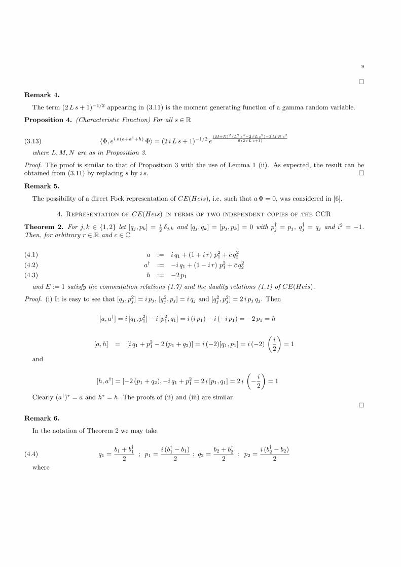
Remark 4.

The term (2Ls+ 1)−1/2 appearing in (3.11) is the moment generating function of a gamma random variable.

Proposition 4. (Characteristic Function) For all s ∈ R

(3.13) 〈Φ, ei s (a+a†+h) Φ〉 = (2 i L s+ 1)−1/2 e(M+N)2 (L2 s4−2 i L s3)−3M N s2

6 (2 i L s+1)

where L,M,N are as in Proposition 3.

Proof. The proof is similar to that of Proposition 3 with the use of Lemma 1 (ii). As expected, the result can beobtained from (3.11) by replacing s by i s. �

Remark 5.

The possibility of a direct Fock representation of CE(Heis), i.e. such that aΦ = 0, was considered in [6].

4. Representation of CE(Heis) in terms of two independent copies of the CCR

Theorem 2. For j, k ∈ {1, 2} let [qj , pk] = i2 δj,k and [qj , qk] = [pj , pk] = 0 with p†j = pj, q

†j = qj and i2 = −1.

Then, for arbitrary r ∈ R and c ∈ C

a := i q1 + (1 + i r) p21 + c q2

2(4.1)

a† := −i q1 + (1− i r) p21 + c q2

2(4.2)

h := −2 p1(4.3)

and E := 1 satisfy the commutation relations (1.7) and the duality relations (1.1) of CE(Heis).

Proof. (i) It is easy to see that [qj , p2j ] = i pj , [q2

j , pj ] = i qj and [q2j , p

2j ] = 2 i pj qj . Then

[a, a†] = i [q1, p21]− i [p2

1, q1] = i (i p1)− i (−i p1) = −2 p1 = h

[a, h] = [i q1 + p21 − 2 (p1 + q2)] = i (−2)[q1, p1] = i (−2)

(i

2

)= 1

and

[h, a†] = [−2 (p1 + q2),−i q1 + p21 = 2 i [p1, q1] = 2 i

(− i

2

)= 1

Clearly (a†)∗ = a and h∗ = h. The proofs of (ii) and (iii) are similar.�

Remark 6.

In the notation of Theorem 2 we may take

(4.4) q1 =b1 + b†1

2; p1 =

i (b†1 − b1)

2; q2 =

b2 + b†22

; p2 =i (b†2 − b2)

2

where

10

(4.5) [b1, b†1] = [b2, b

†2] = 1 ; [b†1, b

†2] = [b1, b2] = [b1, b

†2] = [b†1, b2] = 0

In that case Theorem 3 would extend to the product of the moment generating functions of two independentrandom variables defined in terms of the generators of two mutually commuting Schrodinger algebras.

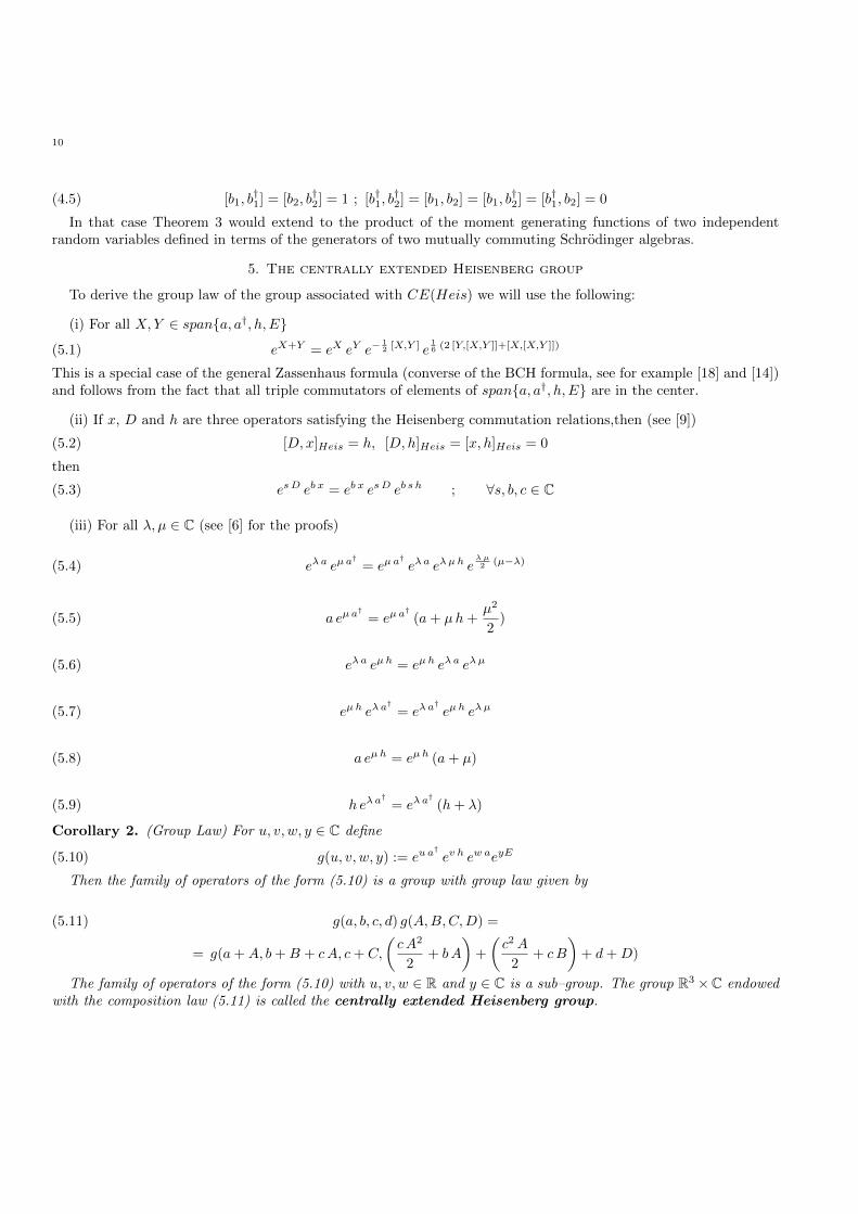
5. The centrally extended Heisenberg group

To derive the group law of the group associated with CE(Heis) we will use the following:

(i) For all X,Y ∈ span{a, a†, h, E}

(5.1) eX+Y = eX eY e−12 [X,Y ] e

16 (2 [Y,[X,Y ]]+[X,[X,Y ]])

This is a special case of the general Zassenhaus formula (converse of the BCH formula, see for example [18] and [14])and follows from the fact that all triple commutators of elements of span{a, a†, h, E} are in the center.

(ii) If x, D and h are three operators satisfying the Heisenberg commutation relations,then (see [9])

(5.2) [D,x]Heis = h, [D,h]Heis = [x, h]Heis = 0

then

(5.3) esD eb x = eb x esD eb s h ; ∀s, b, c ∈ C

(iii) For all λ, µ ∈ C (see [6] for the proofs)

(5.4) eλ a eµa†

= eµa†eλ a eλµh e

λµ2 (µ−λ)

(5.5) a eµa†

= eµa†

(a+ µh+µ2

2)

(5.6) eλ a eµh = eµh eλ a eλµ

(5.7) eµh eλ a†

= eλ a†eµh eλµ

(5.8) a eµh = eµh (a+ µ)

(5.9) h eλ a†

= eλ a†

(h+ λ)

Corollary 2. (Group Law) For u, v, w, y ∈ C define

(5.10) g(u, v, w, y) := eu a†ev h ew aeyE

Then the family of operators of the form (5.10) is a group with group law given by

(5.11) g(a, b, c, d) g(A,B,C,D) =

= g(a+A, b+B + cA, c+ C,

(cA2

2+ bA

)+

(c2A

2+ cB

)+ d+D)

The family of operators of the form (5.10) with u, v, w ∈ R and y ∈ C is a sub–group. The group R3 ×C endowedwith the composition law (5.11) is called the centrally extended Heisenberg group.

11

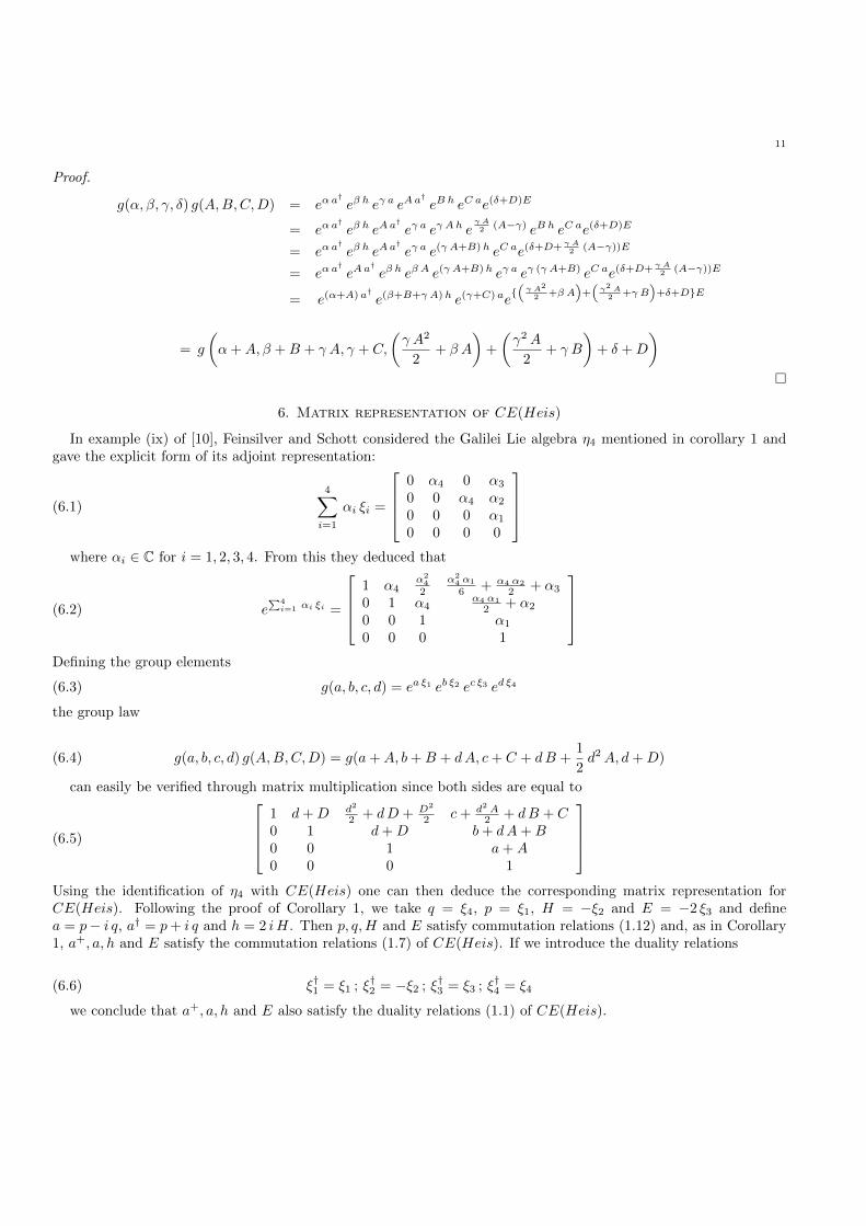
Proof.

g(α, β, γ, δ) g(A,B,C,D) = eαa†eβ h eγ a eAa

†eB h eC ae(δ+D)E

= eαa†eβ h eAa

†eγ a eγ Ah e

γ A2 (A−γ) eB h eC ae(δ+D)E

= eαa†eβ h eAa

†eγ a e(γ A+B)h eC ae(δ+D+ γ A

2 (A−γ))E

= eαa†eAa

†eβ h eβ A e(γ A+B)h eγ a eγ (γ A+B) eC ae(δ+D+ γ A

2 (A−γ))E

= e(α+A) a† e(β+B+γ A)h e(γ+C) ae{(γ A2

2 +β A)

+(γ2 A

2 +γ B)

+δ+D}E

= g

(α+A, β +B + γ A, γ + C,

(γ A2

2+ β A

)+

(γ2A

2+ γ B

)+ δ +D

)�

6. Matrix representation of CE(Heis)

In example (ix) of [10], Feinsilver and Schott considered the Galilei Lie algebra η4 mentioned in corollary 1 andgave the explicit form of its adjoint representation:

(6.1)

4∑i=1

αi ξi =

0 α4 0 α3

0 0 α4 α2

0 0 0 α1

0 0 0 0

where αi ∈ C for i = 1, 2, 3, 4. From this they deduced that

(6.2) e∑4i=1 αi ξi =

1 α4

α24

2α2

4 α1

6 + α4 α2

2 + α3

0 1 α4α4 α1

2 + α2

0 0 1 α1

0 0 0 1

Defining the group elements

(6.3) g(a, b, c, d) = ea ξ1 eb ξ2 ec ξ3 ed ξ4

the group law

(6.4) g(a, b, c, d) g(A,B,C,D) = g(a+A, b+B + dA, c+ C + dB +1

2d2A, d+D)

can easily be verified through matrix multiplication since both sides are equal to

(6.5)

1 d+D d2

2 + dD + D2

2 c+ d2 A2 + dB + C

0 1 d+D b+ dA+B0 0 1 a+A0 0 0 1

Using the identification of η4 with CE(Heis) one can then deduce the corresponding matrix representation forCE(Heis). Following the proof of Corollary 1, we take q = ξ4, p = ξ1, H = −ξ2 and E = −2 ξ3 and definea = p− i q, a† = p+ i q and h = 2 iH. Then p, q,H and E satisfy commutation relations (1.12) and, as in Corollary1, a+, a, h and E satisfy the commutation relations (1.7) of CE(Heis). If we introduce the duality relations

(6.6) ξ†1 = ξ1 ; ξ†2 = −ξ2 ; ξ†3 = ξ3 ; ξ†4 = ξ4

we conclude that a+, a, h and E also satisfy the duality relations (1.1) of CE(Heis).

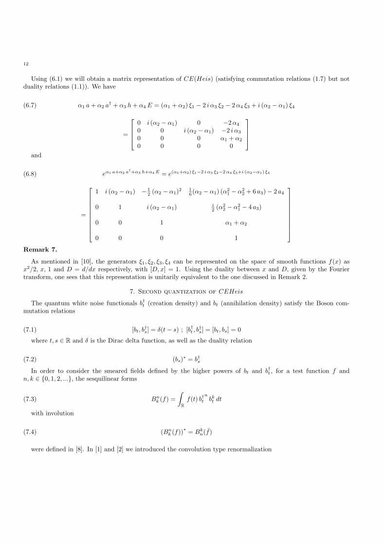
12

Using (6.1) we will obtain a matrix representation of CE(Heis) (satisfying commutation relations (1.7) but notduality relations (1.1)). We have

(6.7) α1 a+ α2 a† + α3 h+ α4E = (α1 + α2) ξ1 − 2 i α3 ξ2 − 2α4 ξ3 + i (α2 − α1) ξ4

=

0 i (α2 − α1) 0 −2α4

0 0 i (α2 − α1) −2 i α3

0 0 0 α1 + α2

0 0 0 0

and

(6.8) eα1 a+α2 a†+α3 h+α4 E = e(α1+α2) ξ1−2 i α3 ξ2−2α4 ξ3+i (α2−α1) ξ4

=

1 i (α2 − α1) − 12 (α2 − α1)2 1

6 (α2 − α1) (α21 − α2

2 + 6 a3)− 2 a4

0 1 i (α2 − α1) i2 (α2

2 − α21 − 4 a3)

0 0 1 α1 + α2

0 0 0 1

Remark 7.

As mentioned in [10], the generators ξ1, ξ2, ξ3, ξ4 can be represented on the space of smooth functions f(x) asx2/2, x, 1 and D = d/dx respectively, with [D,x] = 1. Using the duality between x and D, given by the Fouriertransform, one sees that this representation is unitarily equivalent to the one discussed in Remark 2.

7. Second quantization of CEHeis

The quantum white noise functionals b†t (creation density) and bt (annihilation density) satisfy the Boson com-mutation relations

(7.1) [bt, b†s] = δ(t− s) ; [b†t , b

†s] = [bt, bs] = 0

where t, s ∈ R and δ is the Dirac delta function, as well as the duality relation

(7.2) (bs)∗ = b†s

In order to consider the smeared fields defined by the higher powers of bt and b†t , for a test function f andn, k ∈ {0, 1, 2, ...}, the sesquilinear forms

(7.3) Bnk (f) =

∫Rf(t) b†t

nbkt dt

with involution

(7.4) (Bnk (f))∗

= Bkn(f)

were defined in [8]. In [1] and [2] we introduced the convolution type renormalization

13

(7.5) δl(t− s) = δ(s) δ(t− s) ; l = 2, 3, ....

of the higher powers of the Dirac delta function, and by restricting to test functions f(t) such that f(0) = 0 weobtained the RHPWN ∗–Lie algebra commutation relations

(7.6) [Bnk (f), BNK (g)]RHPWN = (kN −K n) Bn+N−1k+K−1 (f g)

The easily checked commutation relations

[B01(f)−B1

0(f), B01(g) +B1

0(g)] = 2B00(f g)(7.7)

[B02(f) +B2

0(f)− 2B11(f)−B0

0(f), B01(g) +B1

0(g)] = 4(B0

1(f g)−B10(f g)

)(7.8)

allow us to immediately extend the proof of Theorem 1 and realize the second quantized CEHeis commutationrelations

[a(f), a†(g)]CE(Heis) = h(f g)(7.9)

[h(f), a†(g)]CE(Heis) = E(f g)(7.10)

[a(f), h(g)]CE(Heis) = E(f g)(7.11)

as well as the duality relations

(7.12) a(f)∗

= a†(f) ; h(f)∗

= h(f) ; E(f)∗

= E(f)

in terms of the first and second order RHPWN generators B02 , B2

0 , B11 , B0

1 , B10 , and B0

0 .

Theorem 3. (RHPWN representation of CE(Heis)) Let f, g be arbitrary test functions as in (7.6). For arbitraryρ, r ∈ R with r 6= 0:

a(f) = −(r2

4− i ρ

) (B0

2(f) +B20(f)− 2B1

1(f)−B00(f)

)− i

2 r

(B0

1(f) +B10(f)

)(7.13)

a†(f) = −(r2

4+ i ρ

) (B0

2(f) +B20(f)− 2B1

1(f)−B00(f)

)+

i

2 r

(B0

1(f) +B10(f)

)(7.14)

h(f) = i r(B1

0(f)−B01(f)

)(7.15)

E(f) = B00(f)(7.16)

satisfy the second quantized CEHeis commutation relations (7.10)-(7.11) and the duality relations (7.12) above.

Proof. The proof is similar to that of theorem 1. �

References

[1] Accardi, L., Boukas, A.: Renormalized higher powers of white noise (RHPWN) and conformal field theory, Infinite DimensionalAnalysis, Quantum Probability, and Related Topics 9, No. 3, (2006) 353–360.

[2] Accardi, L., Boukas, A.: The emergence of the Virasoro and w∞ Lie algebras through the renormalized higher powers of quantumwhite noise , International Journal of Mathematics and Computer Science, 1, No.3, (2006) 315–342.

[3] Accardi, L., Boukas, A.: Fock representation of the renormalized higher powers of white noise and the Virasoro–Zamolodchikov–w∞∗–Lie algebra, J. Phys. A: Math. Theor., 41 (2008).

[4] Accardi, L., Boukas, A.: Cohomology of the Virasoro–Zamolodchikov and Renormalized Higher Powers of White Noise ∗–Lie algebras,Infinite Dimensional Anal. Quantum Probab. Related Topics, Vol. 12, No. 2 (2009) 1-20.

14

[5] Accardi, L., Boukas, A.: Quantum probability, renormalization and infinite dimensional ∗–Lie algebras, SIGMA (Symmetry, Inte-grability and Geometry: Methods and Applications), 5 (2009), 056, 31 pages.

[6] Accardi, L., Boukas, A.: On the Fock representation of the central extensions of the Heisenberg algebra, to appear in Australian

Journal of Mathematical Analysis and Applications.[7] Accardi, L., Boukas, A., Franz, U.: Renormalized powers of quantum white noise, Infinite Dimensional Analysis, Quantum Proba-

bility, and Related Topics, Vol. 9, No. 1 (2006), 129–147.

[8] Accardi L., Lu Y. G., Volovich I. V.: White noise approach to classical and quantum stochastic calculi, Lecture Notes of the VolterraInternational School of the same title, Trento, Italy (1999), Volterra Center preprint 375, Universita di Roma Tor Vergata.

[9] Feinsilver, P. J., Schott, R.: Algebraic structures and operator calculus. Volumes I and III, Kluwer, 1993.[10] Feinsilver, P. J., Schott, R.: Differential relations and recurrence formulas for representations of Lie groups, Stud. Appl. Math., 96

(1996), no. 4, 387–406.

[11] Feinsilver, P. J., Giering, M., Kocik, J.: Canonical variables and analysis on so(n, 2), Journal of Physics: A Mathematical, 34 (2001),pp 2367–2376

[12] Feinsilver, P. J., Kocik, J., Schott, R.: Representations of the Schroedinger algebra and Appell systems, Fortschr. Phys. 52 (2004),

no. 4, 343–359.[13] Feinsilver, P. J., Kocik, J., Schott, R.: Berezin quantization of the Schrodinger algebra, Infinite Dimensional Analysis, Quantum

Probability, and Related Topics, Vol. 6, No. 1 (2003), 57–71.

[14] Fuchs, J., Schweigert C. : Symmetries, Lie Algebras and Representations (A graduate course for physicists), Cambridge Monographson Mathematical Physics, Cambridge University Press, 1997.

[15] Kruchkovich, G. I.: : Classification of three-dimensional Riemannian spaces according to groups of motions, UMN, 9:1(59) (1954),

3-40 Usp. Mat. Nauk. 9 59 (1954)[16] Ovando, G.: Four dimensional symplectic Lie algebras, Beitrage Algebra Geom. 47 (2006), no. 2, 419–434.

[17] Snobl, L., Winternitz, P.: A class of solvable Lie algebras and their Casimir Invariants, arXiv:math-ph/0411023v1 4 Nov 2004

[18] Suzuki, M.: On the convergence of exponential operators—the Zassenhaus formula, BCH formula and systematic approximants,Comm. Math. Phys. 57 (1997), no. 3, 193–200.