The Complexity of Generalized Satisfiability for Linear Temporal Logic

Logical Methods in Computer ScienceVol. 5 (1:1) 2009, pp. 1–1–21www.lmcs-online.org

Submitted Mar. 28, 2008Published Jan. 26, 2009

THE COMPLEXITY OF GENERALIZED SATISFIABILITY

FOR LINEAR TEMPORAL LOGIC

MICHAEL BAULAND a, THOMAS SCHNEIDER b, HENNING SCHNOOR c, ILKA SCHNOOR d,AND HERIBERT VOLLMER e

a Knipp GmbH, Martin-Schmeißer-Weg 9, 44227 Dortmund, Germanye-mail address: [email protected]

b School of Computer Science, University of Manchester, Oxford Road, Manchester M13 9PL, UKe-mail address: [email protected]

c Inst. fur Informatik, Christian-Albrechts-Universitat zu Kiel, 24098 Kiel, Germanye-mail address: [email protected]

d Inst. fur Theoretische Informatik, Universitat zu Lubeck, Ratzeburger Allee 160, 23538 Lubeck,Germanye-mail address: [email protected]

e Inst. fur Theoretische Informatik, Universitat Hannover, Appelstr. 4, 30167 Hannover, Germanye-mail address: [email protected]

Abstract. In a seminal paper from 1985, Sistla and Clarke showed that satisfiabilityfor Linear Temporal Logic (LTL) is either NP-complete or PSPACE-complete, dependingon the set of temporal operators used. If, in contrast, the set of propositional operatorsis restricted, the complexity may decrease. This paper undertakes a systematic study ofsatisfiability for LTL formulae over restricted sets of propositional and temporal opera-tors. Since every propositional operator corresponds to a Boolean function, there existinfinitely many propositional operators. In order to systematically cover all possible setsof them, we use Post’s lattice. With its help, we determine the computational complexityof LTL satisfiability for all combinations of temporal operators and all but two classesof propositional functions. Each of these infinitely many problems is shown to be eitherPSPACE-complete, NP-complete, or in P.

2000 ACM Subject Classification: F.4.1.Key words and phrases: computational complexity, linear temporal logic, satisfiability.

∗ This article extends the conference contribution [BSS+07] with full proofs of all lemmata and theorems.Supported by the Postdoc Programme of the German Academic Exchange Service (DAAD).Supported in part by DFG VO 630/6-1.

LOGICAL METHODSl IN COMPUTER SCIENCE DOI:10.2168/LMCS-5 (1:1) 2009c© M. Bauland, T. Schneider, H. Schnoor, I. Schnoor, and H. VollmerCC© Creative Commons

http://creativecommons.org/about/licenses

2 M. BAULAND, T. SCHNEIDER, H. SCHNOOR, I. SCHNOOR, AND H. VOLLMER

1. Introduction

Linear Temporal Logic (LTL) was introduced by Pnueli in [Pnu77] as a formalism for rea-soning about the properties and the behaviors of parallel programs and concurrent systems,and has widely been used for these purposes. Because of the need to perform reasoningtasks—such as deciding satisfiability, validity, or truth in a structure generated by binaryrelations—in an automated manner, their decidability and computational complexity is animportant issue.

It is known that in the case of full LTL with the operators F (eventually), G (invariantly),X (next-time), U (until), and S (since), satisfiability and determination of truth are PSPACE-complete [SC85]. Restricting the set of temporal operators leads to NP-completeness insome cases [SC85]. These results imply that reasoning with LTL is difficult in terms ofcomputational complexity.

This raises the question under which restrictions the complexity of these problemsdecreases. Contrary to classical modal logics, there does not seem to be a natural way tomodify the semantics of LTL and obtain decision problems with lower complexity. However,there are several possible constraints that can be posed on the syntax. One possibility is torestrict the set of temporal operators, which has been done exhaustively in [SC85, Mar04].

Another constraint is to allow only a certain “degree of propositionality” in the lan-guage, i.e., to restrict the set of allowed propositional operators. Every propositional op-erator represents a Boolean function—e.g., the operator ∧ (and) corresponds to the binaryfunction whose value is 1 if and only if both arguments have value 1. There are infinitelymany Boolean functions and hence an infinite number of propositional operators.

We will consider propositional restrictions in a systematic way, achieving a completeclassification of the complexity of the reasoning problems for LTL. Not only will this revealall cases in this framework where satisfiability is tractable. It will also provide a betterinsight into the sources of hardness by explicitly stating the combinations of temporaland propositional operators that lead to NP- or PSPACE-hard fragments. In addition, the“sources of hardness” will be identified whenever a proof technique is not transferable froman easy to a hard fragment.

Related work. The complexity of model-checking and satisfiability problems for several syn-tactic restrictions of LTL fragments has been determined in the literature: In [SC85, Mar04],temporal operators and the use of negation have been restricted; these fragments have beenshown to be NP- or PSPACE-complete. In [DS02], temporal operators, their nesting, andthe number of atomic propositions have been restricted; these fragments have been shown tobe tractable or NP-complete. Furthermore, due to [CL93, DFR00], the restriction to Hornformulae does not decrease the complexity of satisfiability for LTL. As for related logics, thecomplexity of satisfiability has been shown in [EES90] to be tractable or NP-complete forthree fragments of CTL (computation tree logic) with temporal and propositional restric-tions. In [Hal95], satisfiability for multimodal logics has been investigated systematically,bounding the depth of modal operators and the number of atomic propositions. In [Hem01],it was shown that satisfiability for modal logic over linear frames drops from NP-completeto tractable if propositional operators are restricted to conjunction and atomic negation.

The effect of propositional restrictions on the complexity of the satisfiability problemwas first considered systematically by Lewis for the case of classical propositional logicin [Lew79]. He established a dichotomy—depending on the set of propositional operators,satisfiability is either NP-complete or decidable in polynomial time. In the case of modal

THE COMPLEXITY OF GENERALIZED SATISFIABILITY FOR LTL 3

propositional logic, a trichotomy has been achieved in [BHSS06]: modal satisfiability isPSPACE-complete, coNP-complete, or in P. That complete classification in terms of restric-tions on the propositional operators follows the structure of Post’s lattice of closed sets ofBoolean functions [Pos41].

Our contribution. This paper analyzes the same systematic propositional restrictions forLTL, and combines them with restrictions on the temporal operators. Using Post’s lattice,we examine the satisfiability problem for every possible fragment of LTL determined byan arbitrary set of propositional operators and any subset of the five temporal operatorslisted above. We determine the computational complexity of these problems, except for onecase—where only propositional operators based on the binary xor function (and, perhaps,constants) are allowed. We show that all remaining cases are either PSPACE-complete,NP-complete, or in P.

It is not the aim of this paper to focus on particular propositional restrictions thatare motivated by certain applications. We prefer to give a classification as complete aspossible which allows to choose a fragment that is appropriate, in terms of expressivity andtractability, for any given application. Applications of syntactically restricted fragmentsof temporal logics can be found, for example, in the study of cryptographic protocols: In[Low08], Gavin Lowe restricts the application of negation and temporal operators to obtainpractical verification algorithms.

Among our results, we exhibit cases with non-trivial tractability as well as the smallestpossible sets of propositional and temporal operators that already lead to NP-completenessor PSPACE-completeness, respectively. Examples for the first group are cases in which onlythe unary not function, or only monotone functions are allowed, but there is no restriction onthe temporal operators. As for the second group, if only the binary function f with f(x, y) =(x ∧ y) is permitted, then satisfiability is NP-complete already in the case of propositionallogic [Lew79]. Our results show that the presence of the same function f separates thetractable languages from the NP-complete and PSPACE-complete ones, depending on theset of temporal operators used. According to this, minimal sets of temporal operatorsleading to PSPACE-completeness together with f are, for example, {U} and {F,X}.

The technically most involved proof is that of PSPACE-hardness for the language withonly the temporal operator S and the boolean operator f (Theorem 3.3). The difficultylies in simulating the quantifier tree of a Quantified Boolean Formula (QBF) in a linearstructure.

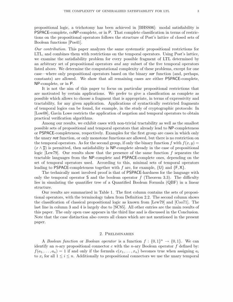
Our results are summarized in Table 1. The first column contains the sets of proposi-tional operators, with the terminology taken from Definition 2.2. The second column showsthe classification of classical propositional logic as known from [Lew79] and [Coo71]. Thelast line in column 3 and 4 is largely due to [SC85]. All other entries are the main results ofthis paper. The only open case appears in the third line and is discussed in the Conclusion.Note that the case distinction also covers all clones which are not mentioned in the presentpaper.

2. Preliminaries

A Boolean function or Boolean operator is a function f : {0, 1}n → {0, 1}. We canidentify an n-ary propositional connector c with the n-ary Boolean operator f defined by:f(a1, . . . , an) = 1 if and only if the formula c(x1, . . . , xn) becomes true when assigning ai

to xi for all 1 ≤ i ≤ n. Additionally to propositional connectors we use the unary temporal


set of temporal operators ∅ {F}, {G}, any other

set of propositional operators {F,G}, {X} combination

all operators 1-reproducing or self-dual trivial trivial trivial

only negation or all operators monotone in P in P in P

all operators linear in P ? ?

x ∧ ¬y is expressible NP-c. NP-c. PSPACE-c.

all Boolean functions NP-c. NP-c. PSPACE-c.

Table 1: Complexity results for satisfiability. The entries “trivial” denote cases in which agiven formula is always satisfiable. The abbreviation “c.” stands for “complete.”Question marks stand for open questions.

operators X (next-time), F (eventually), G (invariantly) and the binary temporal operatorsU (until), and S (since).

Let B be a finite set of Boolean functions and M be a set of temporal operators.A temporal B-formula over M is a formula ϕ that is built from variables, propositionalconnectors from B, and temporal operators from M . More formally, a temporal B-formulaover M is either a propositional variable or of the form f(ϕ1, . . . , ϕn) or g(ϕ1, . . . , ϕm),where ϕi are temporal B-formulae over M , f is an n-ary propositional operator from B

and g is an m-ary temporal operator from M . In [SC85], complexity results for formulaeusing the temporal operators F, G, X (unary), and U, S (binary) were presented. We extendthese results to temporal B-formulae over subsets of those temporal operators. The setof variables appearing in ϕ is denoted by Vϕ. If M = {X,F,G,U,S} we call ϕ a temporalB-formula, and if M = ∅ we call ϕ a propositional B-formula or simply a B-formula. Theset of all temporal B-formulae over M is denoted by L(M,B).

A model in linear temporal logic is a linear structure of states, which intuitively canbe seen as different points of time, with propositional assignments. Formally a structureS = (s, V, ξ) consists of an infinite sequence s = (si)i∈N of distinct states, a set of variablesV , and a function ξ : {si | i ∈ N} → 2V which induces a propositional assignment of V foreach state. be a structure and ϕ a temporal {∧,¬}-formula over {X,U,S} with variablesfrom V . We define what it means that S satisfies ϕ in si (S, si � ϕ): For a temporal {∧,¬}-formula over {X,U,S} with variables from V we define what it means that S satisfies ϕin si (S, si � ϕ): let ϕ1 and ϕ2 be temporal {∧,¬}-formulae over {X,U,S} and x ∈ V avariable.

S, si � x if and only if x ∈ ξ(si),S, si � ϕ1 ∧ ϕ2 if and only if S, si � ϕ1 and S, si � ϕ2,S, si � ¬ϕ1 if and only if S, si 2 ϕ1,S, si � Xϕ1 if and only if S, si+1 � ϕ1,S, si � ϕ1Uϕ2 if and only if there is a k ≥ i such that S, sk � ϕ2,

and for every i ≤ j < k, S, sj � ϕ1,S, si � ϕ1Sϕ2 if and only if there is a k ≤ i such that S, sk � ϕ2,

and for every k < j ≤ i, S, sj � ϕ1.

The remaining temporal operators are interpreted as abbreviations: Fϕ = trueUϕ andGϕ = ¬F¬ϕ. Therefore and since every Boolean operator can be composed from ∧ and


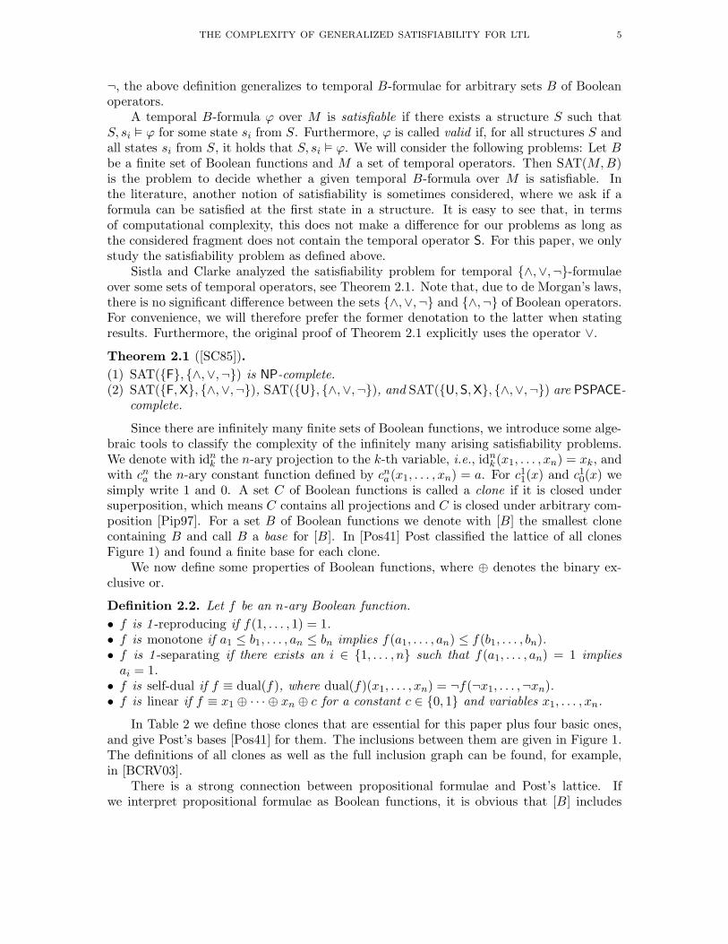
¬, the above definition generalizes to temporal B-formulae for arbitrary sets B of Booleanoperators.

A temporal B-formula ϕ over M is satisfiable if there exists a structure S such thatS, si � ϕ for some state si from S. Furthermore, ϕ is called valid if, for all structures S andall states si from S, it holds that S, si � ϕ. We will consider the following problems: Let Bbe a finite set of Boolean functions and M a set of temporal operators. Then SAT(M,B)is the problem to decide whether a given temporal B-formula over M is satisfiable. Inthe literature, another notion of satisfiability is sometimes considered, where we ask if aformula can be satisfied at the first state in a structure. It is easy to see that, in termsof computational complexity, this does not make a difference for our problems as long asthe considered fragment does not contain the temporal operator S. For this paper, we onlystudy the satisfiability problem as defined above.

Sistla and Clarke analyzed the satisfiability problem for temporal {∧,∨,¬}-formulaeover some sets of temporal operators, see Theorem 2.1. Note that, due to de Morgan’s laws,there is no significant difference between the sets {∧,∨,¬} and {∧,¬} of Boolean operators.For convenience, we will therefore prefer the former denotation to the latter when statingresults. Furthermore, the original proof of Theorem 2.1 explicitly uses the operator ∨.

Theorem 2.1 ([SC85]).

(1) SAT({F}, {∧,∨,¬}) is NP-complete.(2) SAT({F,X}, {∧,∨,¬}), SAT({U}, {∧,∨,¬}), and SAT({U,S,X}, {∧,∨,¬}) are PSPACE-

complete.

Since there are infinitely many finite sets of Boolean functions, we introduce some alge-braic tools to classify the complexity of the infinitely many arising satisfiability problems.We denote with idn

k the n-ary projection to the k-th variable, i.e., idnk(x1, . . . , xn) = xk, and

with cna the n-ary constant function defined by cna(x1, . . . , xn) = a. For c11(x) and c10(x) wesimply write 1 and 0. A set C of Boolean functions is called a clone if it is closed undersuperposition, which means C contains all projections and C is closed under arbitrary com-position [Pip97]. For a set B of Boolean functions we denote with [B] the smallest clonecontaining B and call B a base for [B]. In [Pos41] Post classified the lattice of all clonesFigure 1) and found a finite base for each clone.

We now define some properties of Boolean functions, where ⊕ denotes the binary ex-clusive or.

Definition 2.2. Let f be an n-ary Boolean function.

• f is 1 -reproducing if f(1, . . . , 1) = 1.• f is monotone if a1 ≤ b1, . . . , an ≤ bn implies f(a1, . . . , an) ≤ f(b1, . . . , bn).• f is 1 -separating if there exists an i ∈ {1, . . . , n} such that f(a1, . . . , an) = 1 impliesai = 1.

• f is self-dual if f ≡ dual(f), where dual(f)(x1, . . . , xn) = ¬f(¬x1, . . . ,¬xn).• f is linear if f ≡ x1 ⊕ · · · ⊕ xn ⊕ c for a constant c ∈ {0, 1} and variables x1, . . . , xn.

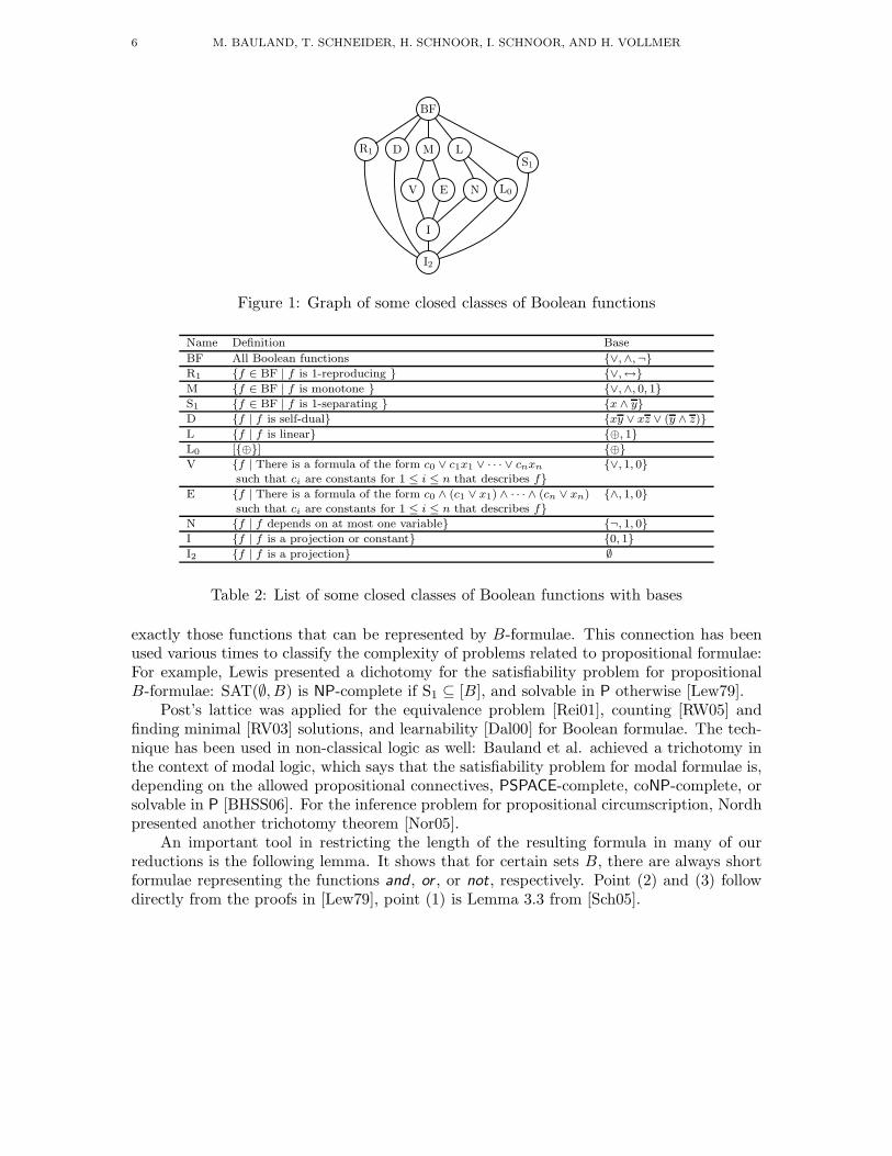
In Table 2 we define those clones that are essential for this paper plus four basic ones,and give Post’s bases [Pos41] for them. The inclusions between them are given in Figure 1.The definitions of all clones as well as the full inclusion graph can be found, for example,in [BCRV03].

There is a strong connection between propositional formulae and Post’s lattice. Ifwe interpret propositional formulae as Boolean functions, it is obvious that [B] includes


R1

BF

MS1

D L

L0V E

I

I2

N

Figure 1: Graph of some closed classes of Boolean functions

Name Definition Base

BF All Boolean functions {∨,∧,¬}

R1 {f ∈ BF | f is 1-reproducing } {∨,↔}

M {f ∈ BF | f is monotone } {∨,∧, 0, 1}

S1 {f ∈ BF | f is 1-separating } {x ∧ y}

D {f | f is self-dual} {xy ∨ xz ∨ (y ∧ z)}

L {f | f is linear} {⊕, 1}

L0 [{⊕}] {⊕}

V {f | There is a formula of the form c0 ∨ c1x1 ∨ · · · ∨ cnxn {∨, 1, 0}such that ci are constants for 1 ≤ i ≤ n that describes f}

E {f | There is a formula of the form c0 ∧ (c1 ∨ x1) ∧ · · · ∧ (cn ∨ xn) {∧, 1, 0}such that ci are constants for 1 ≤ i ≤ n that describes f}

N {f | f depends on at most one variable} {¬, 1, 0}

I {f | f is a projection or constant} {0, 1}

I2 {f | f is a projection} ∅

Table 2: List of some closed classes of Boolean functions with bases

exactly those functions that can be represented by B-formulae. This connection has beenused various times to classify the complexity of problems related to propositional formulae:For example, Lewis presented a dichotomy for the satisfiability problem for propositionalB-formulae: SAT(∅, B) is NP-complete if S1 ⊆ [B], and solvable in P otherwise [Lew79].

Post’s lattice was applied for the equivalence problem [Rei01], counting [RW05] andfinding minimal [RV03] solutions, and learnability [Dal00] for Boolean formulae. The tech-nique has been used in non-classical logic as well: Bauland et al. achieved a trichotomy inthe context of modal logic, which says that the satisfiability problem for modal formulae is,depending on the allowed propositional connectives, PSPACE-complete, coNP-complete, orsolvable in P [BHSS06]. For the inference problem for propositional circumscription, Nordhpresented another trichotomy theorem [Nor05].

An important tool in restricting the length of the resulting formula in many of ourreductions is the following lemma. It shows that for certain sets B, there are always shortformulae representing the functions and , or , or not, respectively. Point (2) and (3) followdirectly from the proofs in [Lew79], point (1) is Lemma 3.3 from [Sch05].


Lemma 2.3.

(1) Let B be a finite set of Boolean functions such that V ⊆ [B] ⊆ M (E ⊆ [B] ⊆ M, resp.).Then there exists a B-formula f(x, y) such that f represents x ∨ y (x ∧ y, resp.) andeach of the variables x and y occurs exactly once in f(x, y).

(2) Let B be a finite set of Boolean functions such that [B] = BF. Then there are B-formulae f(x, y) and g(x, y) such that f represents x ∨ y, g represents x ∧ y, and bothvariables occur in each of these formulae exactly once.

(3) Let B be a finite set of Boolean functions such that N ⊆ [B]. Then there is a B-formulaf(x) such that f represents ¬x and the variable x occurs in f only once.

3. Results

Our proofs for most of the upper complexity bounds will rely on similar ideas as theones in [BHSS06], which are extensions of the proof techniques for the polynomial timeresults in [Lew79]. However, the proof of our polynomial time result for formulae using theexclusive or (Theorem 3.8) will be unrelated to the positive cases for XOR in the mentionedpapers.

The proofs for hardness results will use different techniques. Hardness proofs for uni-modal logics usually work in embedding a tree-like structure directly into a tree-like modelfor modal formulae. Naturally, this approach does not work with LTL which speaks aboutlinear models. Hence, in the proof of Theorem 3.3, we will encode a tree-like structure intoa linear one, and most of the complexity of the proof will come from the need to enforce atree-like behavior of linear models.

3.1. Hard cases. The following lemma gives our general upper bounds for various combi-nations of temporal operators. It establishes that the known upper complexity bounds forthe case where only the propositional operators and , or , and negation are allowed to appearin the formulae still hold for the more general cases that we consider. This does not followtrivially, since there is no obvious strategy that converts every B-formula into a formulausing only the standard connectives without leading to an exponential increase in formulalength. The issues here are similar to the “succinctness gap” between the logics LTL+Pastand LTL discussed in [Mar04]. The proof of Parts (1) and (2) of the following lemma is avariation of the proof for Theorem 3.4 in [BHSS06], where, using a similar reduction, ananalogous result for circuits was proved.

Lemma 3.1. Let B be a finite set of Boolean functions. Then the following holds:

(1) If M ⊆ {F,G,U,S,X}, then SAT(M,B) is in PSPACE,(2) if M ⊆ {F,G}, then SAT(M,B) is in NP, and(3) if M ⊆ {X}, then SAT(M,B) is also in NP.

Proof. For (1), we will show that SAT(M,B) ≤logm SAT({U,S,X} , {∧,∨,¬}), and for (2),

we will show that SAT(M,B) ≤logm SAT({F} , {∧,∨,¬}). The complexity result for these

cases then follows from Theorem 2.1.The construction for (1) and (2) is nearly identical: Let ϕ be a formula with arbitrary

temporal operators and Boolean functions from B. We recursively transform the formulato a new formula using only the Boolean operators ∧, ∨, and ¬, and the temporal operatorsU, S, and X for the first case and the temporal operator F for the second cases. For this we


construct several formulae, which will be connected via conjunction. Let k be the numberof subformulae of ϕ. Accordingly let ϕ1, . . . , ϕk be those subformulae with ϕ = ϕ1. Letx1, . . . , xk be new variables, i.e., distinct from the input variables of ϕ. For all i from 1 tok we make the following case distinction:

• If ϕi = y for a variable y, then let fi(ϕ) = xi ↔ y.• If ϕi = Xϕj, then let fi(ϕ) = xi ↔ Xxj.• If ϕi = Fϕj, then let fi(ϕ) = xi ↔ Fxj.• If ϕi = Gϕj, then let fi(ϕ) = xi ↔ Gxj.• If ϕi = ϕjUϕℓ, then let fi(ϕ) = xi ↔ xjUxℓ.• If ϕi = ϕjSϕℓ, then let fi(ϕ) = xi ↔ xjSxℓ.• If ϕi = g(ϕi1 , . . . , ϕin) for some g ∈ B, then let fi(ϕ) = xi ↔ h(xi1 , . . . , xin), where h is

a formula using only ∧, ∨, and ¬, representing the function g.

Such a formula h always exists with constant length, because the set B is fixed and

does not depend on the input. Now let f(ϕ) = x1∧∧k

i=1(Gfi(ϕ)∧¬(true S¬fi(ϕ))) for case

(1) and f(ϕ) = x1 ∧∧k

i=1 Gfi(ϕ) for case (2). The part Gfi(ϕ) makes sure that fi(ϕ) holdsin every future state of the structure and ¬(trueS¬fi(ϕ))) does the same for the past statesof the structure. Additionally we consider x↔ y as a shorthand for (x∧y)∨ (¬x∧¬y). Forcase (1) we consider Fx as a shorthand for trueUx and Gx as a shorthand for ¬(trueU¬x),and for case (2) we consider Gx as a shorthand for ¬F¬x. Thus we have that f(ϕ) is fromL({U,S,X}, {∧,∨,¬}) in case (1) and from L({F}, {∧,∨,¬}) in case (2). Furthermore fis computable in logarithmic space, because the length of fi is polynomial and neither ↔nor the formulae h occur nested. In order to show that f is the reduction we are lookingfor, we still need to prove that ϕ is satisfiable if and only if f(ϕ) is satisfiable. Assume anarbitrary structure S, such that S, si � f(ϕ) for some si. We first prove by induction onthe structure of the formula that xi holds if and only if ϕi holds in every state s of S (for(1)) respectively in every state which lies in the future of si (for (2)). Therefore for (1) lets be an arbitrary state and for (2) let s be an arbitrary state in the future of si. Thus byconstruction of f(ϕ) the formulae fp(ϕ) hold at s for all 1 ≤ p ≤ k. Then the followingholds:

• If ϕp = y for a variable y, then fp(ϕ) = xp ↔ y and trivially S, s � xp iff S, s � y.• If ϕp = Xϕj , then fp(ϕ) = xp ↔ Xxj. Thus S, s � xp iff for the successor state s′ of s,

we have S, s′ � xj. By induction this is equivalent to S, s′ � ϕj and therefore S, s � ϕp iffS, s � xp.

• The cases for the temporal operator F or G work analogously.• If ϕp = ϕjUϕℓ, then fp(ϕ) = xp ↔ xjUxℓ. Thus S, s � xp iff there exists a state s′ in the

future of s, such that S, s′ � xℓ and in all states sm in between (including s) S, sm � xj .By induction this is equivalent to S, s′ � ϕℓ and for all states in between S, sm � ϕj andtherefore S, s � ϕp iff S, s � xp.

• If ϕp = ϕjSϕℓ, then fp(ϕ) = xp ↔ xjSxℓ. Thus S, s � xp iff there exists a state s′ in thepast of s, such that S, s′ � xℓ and in all states sm in between (including s) S, sm � xj .By induction this is equivalent to S, s′ � ϕℓ and for all states in between S, sm � ϕj andtherefore S, s � ϕp iff S, s � xp.

• If ϕp = g(ϕi1 , . . . , ϕin), then fp(ϕ) = xp ↔ h(xi1 , . . . , xin), where h is a formula usingonly ∧, ∨, and ¬, representing the function g. Thus S, s � xp iff S, s � h(xi1 , . . . , xin). LetI be the subset of In = {i1, . . . , in}, such that S, s � xm for all m ∈ I and S, s � ¬xm forall m ∈ In \ I. By induction S, s � ϕm for all m ∈ I and S, s � ¬ϕm for all m ∈ In \ I and


therefore S, s � h(ϕi1 , . . . , ϕin). Since h represents the function g, we have that S, s � ϕp

iff S, s � xp.

Now, assume that f(ϕ) is satisfiable. Then there exists a structure S, si � f(ϕ) andthus S, si � x1. Since in every state xj holds if and only if ϕj holds, we have that S, si �

ϕ = ϕ1. For the other direction, assume that ϕ is satisfiable. Then there exists a structureS, si � ϕ = ϕ1. Now we can extend S by adding new variables x1, . . . , xk in such a way, thatxj holds in a state s from S if and only if ϕj holds in that state. Call this new structureS′. Then by construction of f(ϕ), we have S′, si � f(ϕ), since in every state xj holds if andonly if ϕj holds. This concludes the proof of the first two cases.

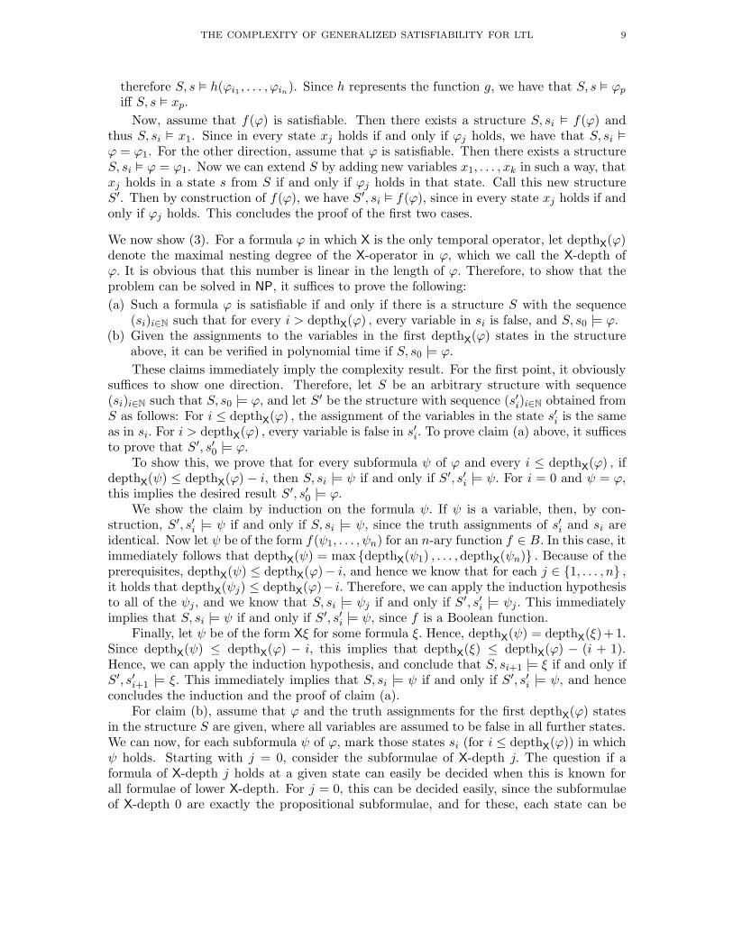
We now show (3). For a formula ϕ in which X is the only temporal operator, let depthX(ϕ)denote the maximal nesting degree of the X-operator in ϕ, which we call the X-depth ofϕ. It is obvious that this number is linear in the length of ϕ. Therefore, to show that theproblem can be solved in NP, it suffices to prove the following:

(a) Such a formula ϕ is satisfiable if and only if there is a structure S with the sequence(si)i∈N such that for every i > depthX(ϕ) , every variable in si is false, and S, s0 |= ϕ.

(b) Given the assignments to the variables in the first depthX(ϕ) states in the structureabove, it can be verified in polynomial time if S, s0 |= ϕ.

These claims immediately imply the complexity result. For the first point, it obviouslysuffices to show one direction. Therefore, let S be an arbitrary structure with sequence(si)i∈N such that S, s0 |= ϕ, and let S′ be the structure with sequence (s′i)i∈N obtained fromS as follows: For i ≤ depthX(ϕ) , the assignment of the variables in the state s′i is the sameas in si. For i > depthX(ϕ) , every variable is false in s′i. To prove claim (a) above, it sufficesto prove that S′, s′0 |= ϕ.

To show this, we prove that for every subformula ψ of ϕ and every i ≤ depthX(ϕ) , ifdepthX(ψ) ≤ depthX(ϕ) − i, then S, si |= ψ if and only if S′, s′i |= ψ. For i = 0 and ψ = ϕ,

this implies the desired result S′, s′0 |= ϕ.

We show the claim by induction on the formula ψ. If ψ is a variable, then, by con-struction, S′, s′i |= ψ if and only if S, si |= ψ, since the truth assignments of s′i and si areidentical. Now let ψ be of the form f(ψ1, . . . , ψn) for an n-ary function f ∈ B. In this case, itimmediately follows that depthX(ψ) = max {depthX(ψ1) , . . . ,depthX(ψn)} . Because of theprerequisites, depthX(ψ) ≤ depthX(ϕ)− i, and hence we know that for each j ∈ {1, . . . , n} ,it holds that depthX(ψj) ≤ depthX(ϕ)− i. Therefore, we can apply the induction hypothesisto all of the ψj , and we know that S, si |= ψj if and only if S′, s′i |= ψj . This immediatelyimplies that S, si |= ψ if and only if S′, s′i |= ψ, since f is a Boolean function.

Finally, let ψ be of the form Xξ for some formula ξ. Hence, depthX(ψ) = depthX(ξ)+1.Since depthX(ψ) ≤ depthX(ϕ) − i, this implies that depthX(ξ) ≤ depthX(ϕ) − (i + 1).Hence, we can apply the induction hypothesis, and conclude that S, si+1 |= ξ if and only ifS′, s′i+1 |= ξ. This immediately implies that S, si |= ψ if and only if S′, s′i |= ψ, and henceconcludes the induction and the proof of claim (a).

For claim (b), assume that ϕ and the truth assignments for the first depthX(ϕ) statesin the structure S are given, where all variables are assumed to be false in all further states.We can now, for each subformula ψ of ϕ, mark those states si (for i ≤ depthX(ϕ)) in whichψ holds. Starting with j = 0, consider the subformulae of X-depth j. The question if aformula of X-depth j holds at a given state can easily be decided when this is known forall formulae of lower X-depth. For j = 0, this can be decided easily, since the subformulaeof X-depth 0 are exactly the propositional subformulae, and for these, each state can be


considered separately. Additionally, observe that in the structure S, all states beyondthe first depthX(ϕ) states satisfy exactly the same set of subformulae of ϕ, hence onlydepthX(ϕ) + 1 many states need to be considered.

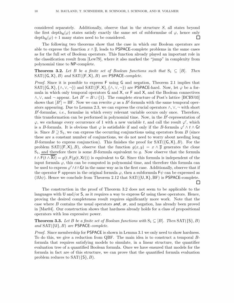
The following two theorems show that the case in which our Boolean operators areable to express the function x ∧ y, leads to PSPACE-complete problems in the same casesas for the full set of Boolean operators. This function already played an important role inthe classification result from [Lew79], where it also marked the “jump” in complexity frompolynomial time to NP-complete.

Theorem 3.2. Let B be a finite set of Boolean functions such that S1 ⊆ [B]. ThenSAT({G,X}, B) and SAT({F,X}, B) are PSPACE-complete.

Proof. Since it is possible to express F using G and negation, Theorem 2.1 implies thatSAT({G,X}, {∧,∨,¬}) and SAT({F,X}, {∧,∨,¬}) are PSPACE-hard. Now, let ϕ be a for-mula in which only temporal operators G and X, or F and X, and the Boolean connectives∧,∨, and ¬ appear. Let B′ = B ∪ {1}. The complete structure of Post’s lattice [BCRV03]shows that [B′] = BF. Now we can rewrite ϕ as a B′-formula with the same temporal oper-ators appearing. Due to Lemma 2.3, we can express the crucial operators ∧,∨,¬ with shortB′-formulae, i.e., formulae in which every relevant variable occurs only once. Therefore,this transformation can be performed in polynomial time. Now, in the B′-representation ofϕ, we exchange every occurrence of 1 with a new variable t, and call the result ϕ′, whichis a B-formula. It is obvious that ϕ is satisfiable if and only if the B-formula ϕ′ ∧ t ∧ Gt

is. Since B ⊇ S1, we can express the occurring conjunctions using operators from B (sincethese are a constant number of conjunctions, we do not need to worry about needing longB-formulae to express conjunction). This finishes the proof for SAT({G,X}, B). For theproblem SAT({F,X}, B), observe that the function g(x, y) = x ∧ y generates the cloneS1, and therefore there is some B-formula equivalent to g. Now observe that the formula

t ∧ F(t ∧ Xt) = g(t,F(g(t,Xt))) is equivalent to Gt. Since this formula is independent of theinput formula ϕ, this can be computed in polynomial time, and therefore this formula canbe used to express ϕ′∧t∧Gt in the same way as in the first case. Additionally, observe that ifthe operator F appears in the original formula ϕ, then a subformula Fψ can be expressed as(1Uψ). Hence we conclude from Theorem 2.12 that SAT({U,X},BF) is PSPACE-complete.

The construction in the proof of Theorem 3.2 does not seem to be applicable to thelanguages with U and/or S, as it requires a way to express Gt using these operators. Hence,proving the desired completeness result requires significantly more work. Note that thecase where B contains the usual operators and , or , and negation, has already been provedin [Mar04]. Our construction shows that hardness already holds for a class of propositionaloperators with less expressive power.

Theorem 3.3. Let B be a finite set of Boolean functions with S1 ⊆ [B]. Then SAT({S}, B)and SAT({U}, B) are PSPACE-complete.

Proof. Since membership for PSPACE is shown in Lemma 3.1 we only need to show hardness.To do this, we give a reduction from QBF. The main idea is to construct a temporal B-formula that requires satisfying models to simulate, in a linear structure, the quantifierevaluation tree of a quantified Boolean formula. Once we have ensured that models for theformula in fact are of this structure, we can prove that the quantified formula evaluationproblem reduces to SAT({S}, B).


First we prove an auxiliary proposition for formulae of a special form which we use asbuilding blocks in the construction. Intuitively the claim states that, given some proposi-tional formulae ϕ1, . . . , ϕn that are pairwise contradictory, we can express that a model hasa subsequence of states such that ϕi holds in the i-th of these states.

We cannot enforce that the i-th state always satisfies the i-th formula, since the truthof an LTL-formula using only S as a temporal operator is invariant under transformationsof models that simply repeat a state finitely many times in the sequence.

Claim 1. Let ϕ1, . . . , ϕn be satisfiable propositional formulae such that ϕi → ¬ϕj is validfor all i, j ∈ {1, . . . , n} with i 6= j. Then the formula

ϕ = ϕ1 ∧ (ϕ1S(ϕ2S(. . . S(ϕn−1Sϕn) . . . ))) ∧ ((. . . ((ϕ1Sϕ2)Sϕ3)S . . . )Sϕn)

is satisfiable and every structure S that satisfies ϕ in a state sm fulfills the following property:there exist natural numbers 0 = a0 < a1 < · · · < an ≤ m+1 such that m−ai < j ≤ m−ai−1

implies S, sj � ϕi for every i ∈ {1 . . . , n}.

Proof. Clearly ϕ is satisfiable: since all formulae ϕi are satisfiable we can find a structureS such that S, si � ϕn−i for all i ∈ {0, . . . , n− 1}. One can verify that S satisfies ϕ in sn−1.

Let S be a structure that satisfies ϕ in a state sm. Since ϕi → ¬ϕj is valid for alli, j ∈ {1, . . . , n} with i 6= j, in every state only one of the formulae ϕi can be satisfiedby S. Therefore and since S, sm � ϕ1S(ϕ2S(. . . S(ϕn−1Sϕn) . . . )) holds, there are naturalnumbers 0 = a0 ≤ a1 ≤ · · · ≤ an−1 < an ≤ m + 1 such that m − ai < l ≤ m − ai−1

implies S, sl � ϕi for every i ∈ {1 . . . , n}. Since S, sm � ϕ1, it holds that a1 > 0. BecauseS, sm � (. . . ((ϕ1Sϕ2)Sϕ3)S . . . )Sϕn we conclude that a1 < · · · < an−1, which proves theclaim. �

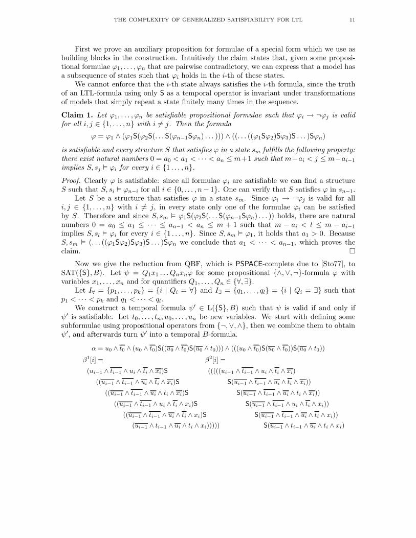
Now we give the reduction from QBF, which is PSPACE-complete due to [Sto77], toSAT({S}, B). Let ψ = Q1x1 . . . Qnxnϕ for some propositional {∧,∨,¬}-formula ϕ withvariables x1, . . . , xn and for quantifiers Q1, . . . , Qn ∈ {∀,∃}.

Let I∀ = {p1, . . . , pk} = {i | Qi = ∀} and I∃ = {q1, . . . , ql} = {i | Qi = ∃} such thatp1 < · · · < pk and q1 < · · · < ql.

We construct a temporal formula ψ′ ∈ L({S}, B) such that ψ is valid if and only ifψ′ is satisfiable. Let t0, . . . , tn, u0, . . . , un be new variables. We start with defining somesubformulae using propositional operators from {¬,∨,∧}, then we combine them to obtainψ′, and afterwards turn ψ′ into a temporal B-formula.

α = u0 ∧ t0 ∧ (u0 ∧ t0)S((u0 ∧ t0)S(u0 ∧ t0))) ∧ (((u0 ∧ t0)S(u0 ∧ t0))S(u0 ∧ t0))

β1[i] =

(ui−1 ∧ ti−1 ∧ ui ∧ ti ∧ xi)S

((ui−1 ∧ ti−1 ∧ ui ∧ ti ∧ xi)S

((ui−1 ∧ ti−1 ∧ ui ∧ ti ∧ xi)S

((ui−1 ∧ ti−1 ∧ ui ∧ ti ∧ xi)S

((ui−1 ∧ ti−1 ∧ ui ∧ ti ∧ xi)S

(ui−1 ∧ ti−1 ∧ ui ∧ ti ∧ xi)))))

β2[i] =

(((((ui−1 ∧ ti−1 ∧ ui ∧ ti ∧ xi)

S(ui−1 ∧ ti−1 ∧ ui ∧ ti ∧ xi))

S(ui−1 ∧ ti−1 ∧ ui ∧ ti ∧ xi))

S(ui−1 ∧ ti−1 ∧ ui ∧ ti ∧ xi))

S(ui−1 ∧ ti−1 ∧ ui ∧ ti ∧ xi))

S(ui−1 ∧ ti−1 ∧ ui ∧ ti ∧ xi)


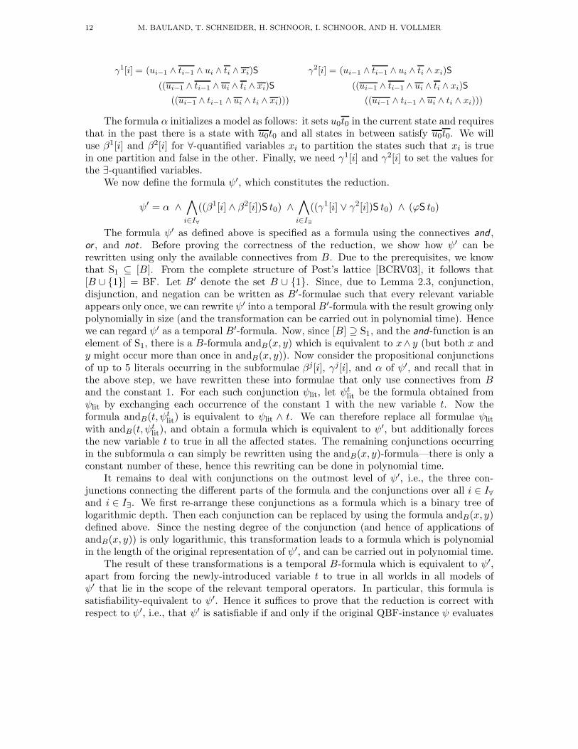
γ1[i] = (ui−1 ∧ ti−1 ∧ ui ∧ ti ∧ xi)S

((ui−1 ∧ ti−1 ∧ ui ∧ ti ∧ xi)S

((ui−1 ∧ ti−1 ∧ ui ∧ ti ∧ xi)))

γ2[i] = (ui−1 ∧ ti−1 ∧ ui ∧ ti ∧ xi)S

((ui−1 ∧ ti−1 ∧ ui ∧ ti ∧ xi)S

((ui−1 ∧ ti−1 ∧ ui ∧ ti ∧ xi)))

The formula α initializes a model as follows: it sets u0t0 in the current state and requiresthat in the past there is a state with u0t0 and all states in between satisfy u0t0. We willuse β1[i] and β2[i] for ∀-quantified variables xi to partition the states such that xi is truein one partition and false in the other. Finally, we need γ1[i] and γ2[i] to set the values forthe ∃-quantified variables.

We now define the formula ψ′, which constitutes the reduction.

ψ′ = α ∧∧

i∈I∀

((β1[i] ∧ β2[i])S t0) ∧∧

i∈I∃

((γ1[i] ∨ γ2[i])S t0) ∧ (ϕS t0)

The formula ψ′ as defined above is specified as a formula using the connectives and ,or , and not. Before proving the correctness of the reduction, we show how ψ′ can berewritten using only the available connectives from B. Due to the prerequisites, we knowthat S1 ⊆ [B]. From the complete structure of Post’s lattice [BCRV03], it follows that[B ∪ {1}] = BF. Let B′ denote the set B ∪ {1}. Since, due to Lemma 2.3, conjunction,disjunction, and negation can be written as B′-formulae such that every relevant variableappears only once, we can rewrite ψ′ into a temporal B′-formula with the result growing onlypolynomially in size (and the transformation can be carried out in polynomial time). Hencewe can regard ψ′ as a temporal B′-formula. Now, since [B] ⊇ S1, and the and-function is anelement of S1, there is a B-formula andB(x, y) which is equivalent to x∧ y (but both x andy might occur more than once in andB(x, y)). Now consider the propositional conjunctionsof up to 5 literals occurring in the subformulae βj[i], γj[i], and α of ψ′, and recall that inthe above step, we have rewritten these into formulae that only use connectives from B

and the constant 1. For each such conjunction ψlit, let ψtlit be the formula obtained from

ψlit by exchanging each occurrence of the constant 1 with the new variable t. Now theformula andB(t, ψt

lit) is equivalent to ψlit ∧ t. We can therefore replace all formulae ψlit

with andB(t, ψtlit), and obtain a formula which is equivalent to ψ′, but additionally forces

the new variable t to true in all the affected states. The remaining conjunctions occurringin the subformula α can simply be rewritten using the andB(x, y)-formula—there is only aconstant number of these, hence this rewriting can be done in polynomial time.

It remains to deal with conjunctions on the outmost level of ψ′, i.e., the three con-junctions connecting the different parts of the formula and the conjunctions over all i ∈ I∀and i ∈ I∃. We first re-arrange these conjunctions as a formula which is a binary tree oflogarithmic depth. Then each conjunction can be replaced by using the formula andB(x, y)defined above. Since the nesting degree of the conjunction (and hence of applications ofandB(x, y)) is only logarithmic, this transformation leads to a formula which is polynomialin the length of the original representation of ψ′, and can be carried out in polynomial time.

The result of these transformations is a temporal B-formula which is equivalent to ψ′,apart from forcing the newly-introduced variable t to true in all worlds in all models ofψ′ that lie in the scope of the relevant temporal operators. In particular, this formula issatisfiability-equivalent to ψ′. Hence it suffices to prove that the reduction is correct withrespect to ψ′, i.e., that ψ′ is satisfiable if and only if the original QBF-instance ψ evaluates


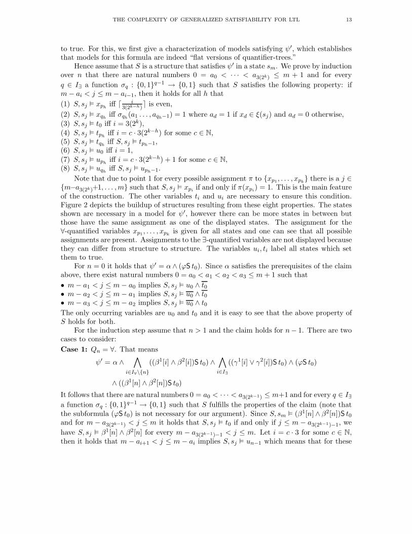
to true. For this, we first give a characterization of models satisfying ψ′, which establishesthat models for this formula are indeed “flat versions of quantifier-trees.”

Hence assume that S is a structure that satisfies ψ′ in a state sm. We prove by inductionover n that there are natural numbers 0 = a0 < · · · < a3(2k) ≤ m + 1 and for every

q ∈ I∃ a function σq : {0, 1}q−1 → {0, 1} such that S satisfies the following property: ifm− ai < j ≤ m− ai−1, then it holds for all h that

(1) S, sj � xphiff ⌈ i

3(2k−h)⌉ is even,

(2) S, sj � xqhiff σqh

(a1 . . . , aqh−1) = 1 where ad = 1 if xd ∈ ξ(sj) and ad = 0 otherwise,

(3) S, sj � t0 iff i = 3(2k),

(4) S, sj � tphiff i = c · 3(2k−h) for some c ∈ N,

(5) S, sj � tqhiff S, sj � tph−1,

(6) S, sj � u0 iff i = 1,

(7) S, sj � uphiff i = c · 3(2k−h) + 1 for some c ∈ N,

(8) S, sj � uqhiff S, sj � uph−1.

Note that due to point 1 for every possible assignment π to {xp1, . . . , xpk

} there is a j ∈{m−a3(2k)+1, . . . ,m} such that S, sj � xpi

if and only if π(xpi) = 1. This is the main feature

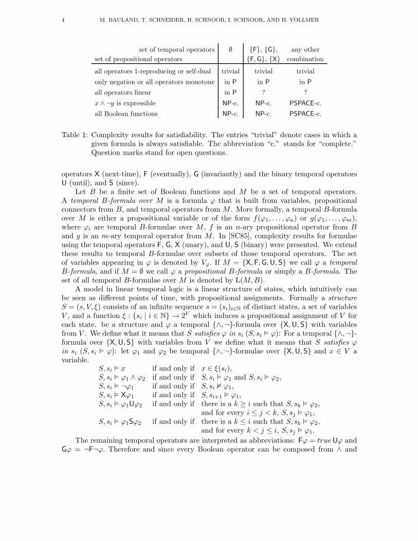
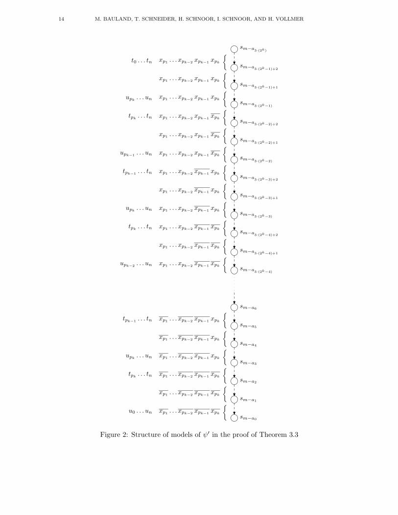
of the construction. The other variables ti and ui are necessary to ensure this condition.Figure 2 depicts the buildup of structures resulting from these eight properties. The statesshown are necessary in a model for ψ′, however there can be more states in between butthose have the same assignment as one of the displayed states. The assignment for the∀-quantified variables xp1

, . . . , xpkis given for all states and one can see that all possible

assignments are present. Assignments to the ∃-quantified variables are not displayed becausethey can differ from structure to structure. The variables ui, ti label all states which setthem to true.

For n = 0 it holds that ψ′ = α∧ (ϕS t0). Since α satisfies the prerequisites of the claimabove, there exist natural numbers 0 = a0 < a1 < a2 < a3 ≤ m+ 1 such that

• m− a1 < j ≤ m− a0 implies S, sj � u0 ∧ t0• m− a2 < j ≤ m− a1 implies S, sj � u0 ∧ t0• m− a3 < j ≤ m− a2 implies S, sj � u0 ∧ t0The only occurring variables are u0 and t0 and it is easy to see that the above property ofS holds for both.

For the induction step assume that n > 1 and the claim holds for n− 1. There are twocases to consider:

Case 1: Qn = ∀. That means

ψ′ = α ∧∧

i∈I∀\{n}

((β1[i] ∧ β2[i])S t0) ∧∧

i∈I∃

((γ1[i] ∨ γ2[i])S t0) ∧ (ϕS t0)

∧ ((β1[n] ∧ β2[n])S t0)

It follows that there are natural numbers 0 = a0 < · · · < a3(2k−1) ≤ m+1 and for every q ∈ I∃

a function σq : {0, 1}q−1 → {0, 1} such that S fulfills the properties of the claim (note thatthe subformula (ϕS t0) is not necessary for our argument). Since S, sm � (β1[n]∧ β2[n])S t0and for m− a3(2k−1) < j ≤ m it holds that S, sj � t0 if and only if j ≤ m− a3(2k−1)−1, we

have S, sj � β1[n] ∧ β2[n] for every m − a3(2k−1)−1 < j ≤ m. Let i = c · 3 for some c ∈ N,then it holds that m− ai+1 < j ≤ m− ai implies S, sj � un−1 which means that for these


sm−a3·(2k)

sm−a3·(2k

−1)+2

sm−a3·(2k

−1)+1

sm−a3·(2k

−1)

sm−a3·(2k

−2)+2

sm−a3·(2k

−2)+1

sm−a3·(2k

−2)

sm−a3·(2k

−3)+2

sm−a3·(2k

−3)+1

sm−a3·(2k

−3)

sm−a3·(2k

−4)+2

sm−a3·(2k

−4)+1

sm−a3·(2k

−4)

sm−a6

sm−a5

sm−a4

sm−a3

sm−a2

sm−a1

sm−a0

{

{

{

{

{

{

{

{

{

{

{

{

{

{

{

{

{

{

xp1 . . . xpk−2xpk−1

xpk


xpk


xpk


xpk


xpk


xpk


xpk


xpk


xpk


xpk


xpk


xpk


xpk


xpk


xpk


xpk


xpk


xpk

t0 . . . tn

upk. . . un

tpk. . . tn

upk−1. . . un

tpk−1. . . tn

upk. . . un

tpk. . . tn

upk−2. . . un

tpk−1. . . tn

upk. . . un

tpk. . . tn

u0 . . . un

Figure 2: Structure of models of ψ′ in the proof of Theorem 3.3


states sj it holds that S, sj � un−1 ∧ tn−1 ∧ un ∧ tn ∧ xn. Due to our proposition there arenatural numbers 0 = bi0 < bi1 < · · · < bi6 ≤ ai + 1 such that

• ai − bi1 < j ≤ ai − bi0 implies S, sj � un−1 ∧ tn−1 ∧ un ∧ tn ∧ xn






The nearest state before sm−aithat satisfies un−1 is sm−ai+1

and the nearest state before

sm−aithat satisfies tn−1 is sm−ai+2

, therefore it holds that bi1 = ai+1−ai and bi5 = ai+2−ai.

By denoting bij + ai with c2i+j we define natural numbers c0, . . . , c3(2k) for which it can beverified that they fulfill the claim.Case 2: Qn = ∃. In this case we have

ψ′ = α ∧∧

i∈I∀

((β1[i] ∧ β2[i])S t0) ∧∧

i∈I∃\{n}

((γ1[i] ∨ γ2[i])S t0) ∧ (ϕS t0)

∧ ((γ1[n] ∨ γ2[n])S t0).

Because of the induction hypothesis there are natural numbers 0 = a0 < a1 < · · · < a3(2k) ≤m+ 1 such that the required properties are satisfied. Analogously to the first case S, sj �

γ1[n]∨γ2[n] is true for every m−a3(2k) < j ≤ m. Let i = c·3, then for m−ai+1 < j ≤ m−ai

it holds that S, sj � un−1 ∧ tn−1 ∧ un ∧ tn ∧ xn or S, sj � un−1 ∧ tn−1 ∧ un ∧ tn ∧ xn, becauseS, sj � un−1. For m− ai+2 < j ≤ m− ai+1 we have that S, sj � un−1 ∧ tn−1 ∧ un ∧ tn ∧ xn

or S, sj � ui−n ∧ ti−n ∧ un ∧ tn ∧ xn and for m − ai+3 < j ≤ m − ai+2 it must holdS, sj � un−1 ∧ tn−1 ∧un ∧ tn ∧xn or S, sj � un−1 ∧ tn−1 ∧un ∧ tn ∧ xn. If S, sai

� γ1[n], thenin all these states xn is satisfied; if S, sai

� γ2[n], then xn is. Therefore with σn defined byσn(d1, . . . , dn−1) = 1 if and only if S, s3(d12n−2+···+dn−120) � γ2[n], the induction is complete,because the binary numbers correspond to the assignments to the ∀-quantified variables.

Note that for a structure that satisfies ψ′ with the above notation, S, sj � ϕ holds for everym− a3(2k) < j ≤ m, since ϕS t0 is a conjunct of ψ′.

Now assume that ψ′ is satisfiable in a state sm of a structure S. This is if and only iffor every q ∈ I∃ there is a function σq : {0, 1}q−1 → {0, 1} such that S fulfills the aboveproperty. Hence each possible assignment J to the ∀-quantified variables {xp1

, . . . , xpk} can

be extended to an assignment to {x1, . . . , xn} by J(xqi) = σqi

(J(x1), . . . , J(xqi−1)) which isequivalent to the validity of ψ. We can prove PSPACE-hardness for SAT({U}, B) with ananalogous construction.

In the following, we use the result from Lewis [Lew79] and the previously establishedupper bounds to obtain NP-completeness results:

Proposition 3.4. Let B be a finite set of Boolean functions such that S1 ⊆ [B]. ThenSAT({F}, B), SAT({G}, B), SAT({F,G}, B), and SAT({X}, B) are NP-complete.

Proof. Trivially, it holds that SAT(∅, B) ≤logm SAT(M,B) for each set M of temporal op-

erators, and SAT(∅, B) is NP-complete due to [Lew79]. The upper bound follows fromTheorem 2.11 and Lemma 3.1.


3.2. Polynomial time results. The following theorem shows that for some sets B ofBoolean functions, there is a satisfying model for every temporal B-formula over any set oftemporal operators. These are the cases where B ⊆ R1, or B ⊆ D. In the first case, everypropositional formula over these operators is satisfied by the assignment giving the value1 to all appearing variables. In the second case, every propositional B-formula describes aself-dual function. For such a formula it holds in particular that if it is not satisfied by theall-zero assignment, then it is satisfied by the all-one assignment. Hence, such formulae arealways satisfiable. It is easy to see that this is also true for temporal formulae involvingthese propositional operators.

Theorem 3.5.

(1) Let B be a finite subset of R1. Then every formula ϕ from L({F, G, X, U, S}, B) issatisfiable.

(2) Let B be a finite subset of D. Then every formula ϕ from L({F,G,X,U,S}, B) is satis-fiable.

Proof.

(1) Since R1 is the class of 1-reproducing Boolean functions, any ψ ∈ R1 is true under theassignment that makes every propositional variable in ψ true. If we apply this fact toformulae ϕ ∈ L({F,G,X,U,S}, B), then it is easy to see that any such formula ϕ is truein every state of a structure Sϕ where the assignment of every state is Vϕ.

(2) We show by induction on the operators that this holds for all formulae. Let S1 (S0)denote the structure where the assignment of every state is Vϕ (∅, resp.) and let s1 (s0,resp.) be the first state. We claim that ϕ ∈ L({F,G,X,U,S}, B) is satisfied by S1 iffϕ is not satisfied by S0. If ϕ is purely propositional the claim holds trivially. We nowhave to look at the following cases:• ϕ = Fϕ1: Assume the claim holds for ϕ1. Since for all states s in S1 the submodel

starting at s are isomorphic, obviously ϕ is satisfied by S1 iff Fϕ is satisfied by S1

and the same argument also holds for S0. Thus S0, s0 2 ϕ iff S1, s1 � ϕ.• ϕ = Gϕ1: This works analogously to F.• ϕ = Xϕ1: This also works analogously to F.• ϕ = ϕ1Uϕ2: Assume the claim holds for ϕ2. Then S0, s0 2 ϕ iff S0, s0 2 ϕ2 iffS1, s1 � ϕ2 iff S1, s1 � ϕ.

• ϕ = ϕ1Sϕ2: This works analogously to U.• ϕ = f(ϕ1, . . . , ϕn), such that f is a self-dual function from B: Assume the claim holds

for ϕi, 1 ≤ i ≤ n, i.e., S1, s1 � ϕi iff S0, s0 2 ϕi. Then S1, s1 2 f(ϕ1, . . . , ϕn) impliesS0, s0 � f(ϕ1, . . . , ϕn) and S1, s1 � f(ϕ1, . . . , ϕn) implies S0, s0 2 f(ϕ1, . . . , ϕn).

The following two theorems prove that satisfiability for formulae with any combinationof modal operators, but only very restricted Boolean operators (i.e., negation and constantsin the first case and only disjunction, conjunction, and constants in the second case), isalways easy to decide.

Theorem 3.6. Let B be a finite subset of N. Then SAT({F,G,X,U,S}, B) can be decidedin polynomial time.

Proof. We give a recursive polynomial-time algorithm deciding the following question: Givena formula ϕ built from propositional negation, constants, variables and arbitrary temporaloperators, which of the following three cases occurs: ϕ is unsatisfiable, ϕ is a tautology,or ϕ is not equivalent to a constant function. We also show that in the latter case, ϕ is


equivalent to a formula using only the above operators in which no constant appears. Wewill call these formulae temporal ¬-formulae.

We give inductive criteria for these cases. Obviously, a constant c is constant, and avariable is not, and can be written in the way defined above. The formula ¬ϕ is equivalentto the constant c if and only if ϕ is equivalent to ¬c, otherwise it is equivalent to a temporal¬-formula. If ϕ = Fϕ1, ϕ = Gϕ1, or ϕ = Xϕ1, then ϕ is equivalent to a constant c if andonly if ϕ1 is equivalent to c : Obviously Fc ≡ Gc ≡ Xc ≡ c for a constant. On the other hand,if ϕ1 is not equivalent to a constant, then due to induction, it is equivalent to a temporal¬-formula. Hence, Fϕ1, Gϕ1 and Xϕ1 are equivalent to temporal ¬-formulae as well, anddue to the proof of Theorem 3.5. 2, these formulae are not equivalent to constants. Hence,if ϕ1 is not equivalent to a constant, then ϕ is not equivalent to a constant either, and canbe written as a temporal ¬-formula.

Now, let ϕ = ϕ1Uϕ2. If ϕ2 is a tautology, i.e., equivalent to the constant 1, then, bythe definition of U, ϕ is a tautology as well. Similarly, if ϕ2 is equivalent to the constant 0,then so is ϕ. Now assume that ϕ2 is not constant. Then, by induction, ϕ2 is equivalent toa temporal ¬-formula. If ϕ1 is equivalent to the constant 0, then ϕ1Uϕ2 is equivalent to ϕ2,and if ϕ1 is equivalent to 1, then ϕ1Uϕ2 is equivalent to Fϕ2. If ϕ1 is not equivalent to aconstant, then, by induction, it can be written as a temporal ¬-formula, and obviously, thisalso holds for ϕ1Uϕ2. Again due to the proof of Theorem 3.5. 2, it follows that the entireformula ϕ is not equivalent to a constant.

For the operator S, a similar argument can be made: Consider the formula ϕ1Sϕ2.If ϕ2 is a constant, then obviously the formula ϕ1Sϕ2 is equivalent to the same constant.If ϕ1 is the constant 0, then ϕ1Sϕ2 is equivalent to ϕ2, and if ϕ1 is the constant 1, thenϕ1Sϕ2 is equivalent to “ϕ2 was true at one point in the past.” If ϕ2 is not a constant,then this is equivalent to ¬ϕ2Sϕ2, and thus this can be written as a temporal ¬-formula aswell. As above, this formula is not equivalent to a constant. Now if both ϕ1 and ϕ2 arenot equivalent to a constant function, then, by induction, both can be written as temporal¬-formulae, and then ϕ1Sϕ2 can be written as such a formula as well. In particular, withanother application of the proof for Theorem 3.5 2, ϕ1Sϕ2 is not equivalent to a constant.

This gives us a recursive algorithm deciding whether ϕ is a constant, and if it is, whichconstant is equivalent to ϕ. The polynomial-time computable function AN is defined asfollows: On input ϕ, AN (ϕ) = c ∈ {0, 1} if ϕ is equivalent to the constant c, and AN (ϕ) isthe symbol NOCONSTANT if ϕ is not equivalent to a constant.

The function can be computed as follows: AN (c) is defined as c. For a variable x,AN (x) is the symbol NOCONSTANT. On input Xϕ, Gϕ, or Fϕ, the algorithm returns AN (ϕ).On input ϕ1Uϕ2, if ϕ2 is a constant c, then AN (ϕ1Uϕ2) = c. Otherwise, if ϕ1 is equivalent to0, then return AN (ϕ2), and if ϕ1 is equivalent to 1, return AN (Fϕ2). If neither ϕ1 nor ϕ2 areconstant, then return the symbol NOCONSTANT. Similarly, on input ϕ1Sϕ2, if ϕ2 is a constantc, then AN (ϕ1Sϕ2) = c. Otherwise, if ϕ1 is the constant 0, then AN (ϕ1Sϕ2) = AN (ϕ2), andif ϕ1 is the constant 1, and ϕ2 is not a constant, then AN (ϕ1Sϕ2) is defined as the symbolNOCONSTANT. If ϕ1 and ϕ2 both are not a constant, then AN (ϕ1Sϕ2) is again defined asthe symbol NOCONSTANT. The function AN can obviously be computed in polynomial time,since there is at most one recursive call for each operator symbol in ϕ.

By the argument above, this algorithm correctly determines if ϕ is equivalent to theconstant 0 or the constant 1. In particular, it determines if a given formula is satisfiable.

Theorem 3.7. Let B be a finite subset of M. Then SAT({F,G,X,U,S}, B) can be decidedin polynomial time.


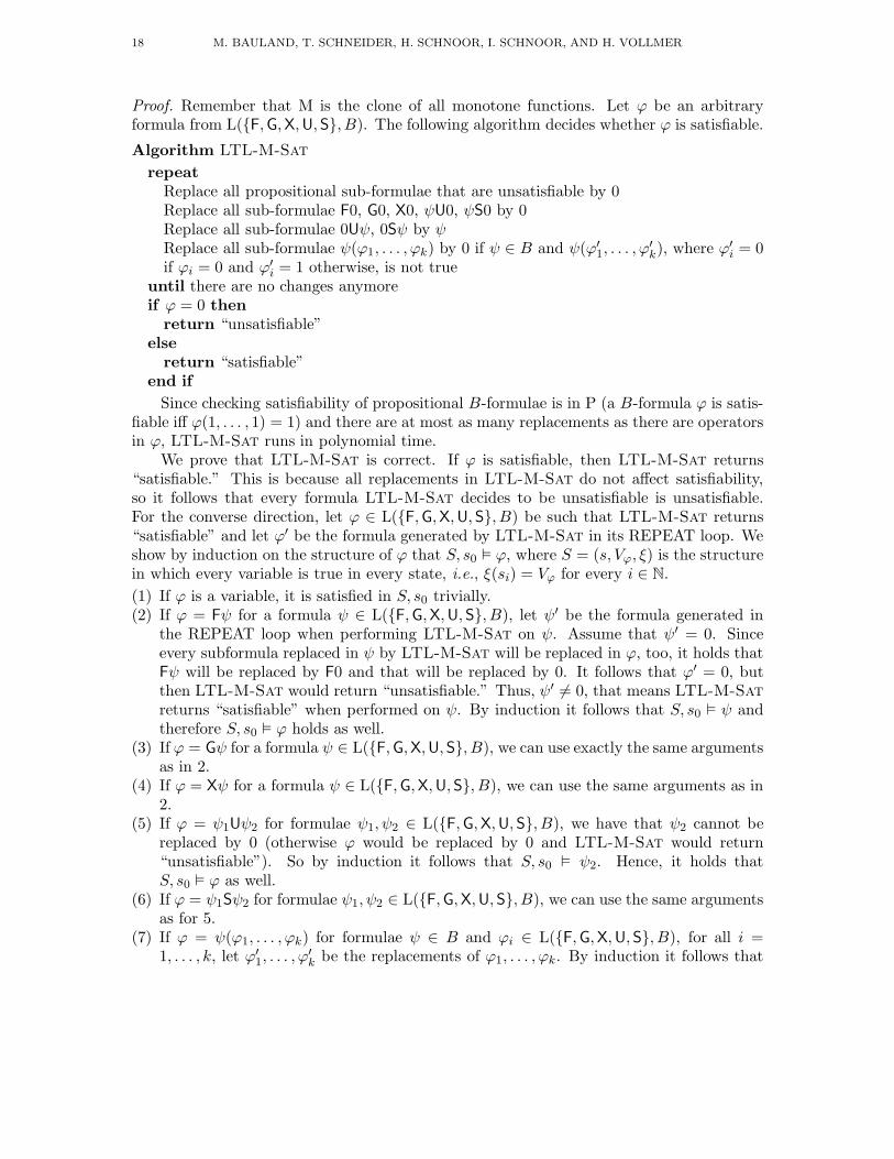
Proof. Remember that M is the clone of all monotone functions. Let ϕ be an arbitraryformula from L({F,G,X,U,S}, B). The following algorithm decides whether ϕ is satisfiable.

Algorithm LTL-M-Sat

repeat

Replace all propositional sub-formulae that are unsatisfiable by 0Replace all sub-formulae F0, G0, X0, ψU0, ψS0 by 0Replace all sub-formulae 0Uψ, 0Sψ by ψReplace all sub-formulae ψ(ϕ1, . . . , ϕk) by 0 if ψ ∈ B and ψ(ϕ′

1, . . . , ϕ′k), where ϕ′

i = 0if ϕi = 0 and ϕ′

i = 1 otherwise, is not trueuntil there are no changes anymoreif ϕ = 0 then

return “unsatisfiable”else

return “satisfiable”end if

Since checking satisfiability of propositional B-formulae is in P (a B-formula ϕ is satis-fiable iff ϕ(1, . . . , 1) = 1) and there are at most as many replacements as there are operatorsin ϕ, LTL-M-Sat runs in polynomial time.

We prove that LTL-M-Sat is correct. If ϕ is satisfiable, then LTL-M-Sat returns“satisfiable.” This is because all replacements in LTL-M-Sat do not affect satisfiability,so it follows that every formula LTL-M-Sat decides to be unsatisfiable is unsatisfiable.For the converse direction, let ϕ ∈ L({F,G,X,U,S}, B) be such that LTL-M-Sat returns“satisfiable” and let ϕ′ be the formula generated by LTL-M-Sat in its REPEAT loop. Weshow by induction on the structure of ϕ that S, s0 � ϕ, where S = (s, Vϕ, ξ) is the structurein which every variable is true in every state, i.e., ξ(si) = Vϕ for every i ∈ N.

(1) If ϕ is a variable, it is satisfied in S, s0 trivially.(2) If ϕ = Fψ for a formula ψ ∈ L({F,G,X,U,S}, B), let ψ′ be the formula generated in

the REPEAT loop when performing LTL-M-Sat on ψ. Assume that ψ′ = 0. Sinceevery subformula replaced in ψ by LTL-M-Sat will be replaced in ϕ, too, it holds thatFψ will be replaced by F0 and that will be replaced by 0. It follows that ϕ′ = 0, butthen LTL-M-Sat would return “unsatisfiable.” Thus, ψ′ 6= 0, that means LTL-M-Sat

returns “satisfiable” when performed on ψ. By induction it follows that S, s0 � ψ andtherefore S, s0 � ϕ holds as well.

(3) If ϕ = Gψ for a formula ψ ∈ L({F,G,X,U,S}, B), we can use exactly the same argumentsas in 2.

(4) If ϕ = Xψ for a formula ψ ∈ L({F,G,X,U,S}, B), we can use the same arguments as in2.

(5) If ϕ = ψ1Uψ2 for formulae ψ1, ψ2 ∈ L({F,G,X,U,S}, B), we have that ψ2 cannot bereplaced by 0 (otherwise ϕ would be replaced by 0 and LTL-M-Sat would return“unsatisfiable”). So by induction it follows that S, s0 � ψ2. Hence, it holds thatS, s0 � ϕ as well.

(6) If ϕ = ψ1Sψ2 for formulae ψ1, ψ2 ∈ L({F,G,X,U,S}, B), we can use the same argumentsas for 5.

(7) If ϕ = ψ(ϕ1, . . . , ϕk) for formulae ψ ∈ B and ϕi ∈ L({F,G,X,U,S}, B), for all i =1, . . . , k, let ϕ′

1, . . . , ϕ′k be the replacements of ϕ1, . . . , ϕk. By induction it follows that


S, s0 � ϕi if and only if ϕ′i 6= 0 for any i ∈ {1, . . . , k}. Since ϕ′ 6= 0 and because of the

last replacement rule, S, s0 � ϕ.

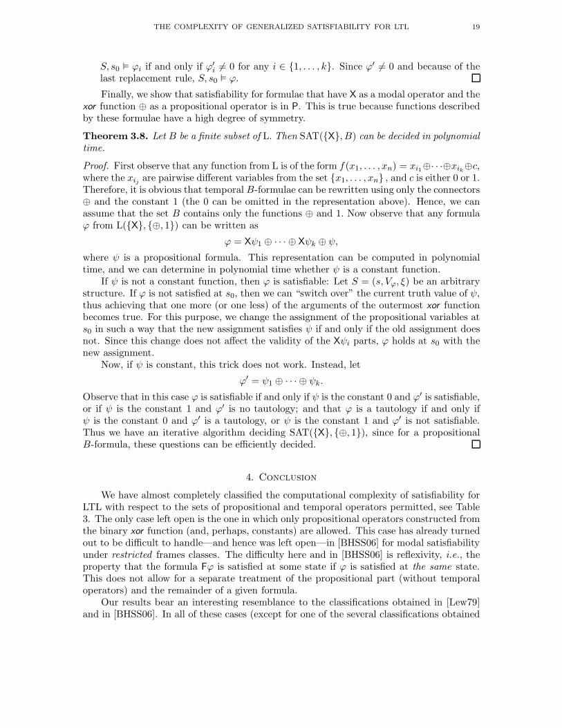
Finally, we show that satisfiability for formulae that have X as a modal operator and thexor function ⊕ as a propositional operator is in P. This is true because functions describedby these formulae have a high degree of symmetry.

Theorem 3.8. Let B be a finite subset of L. Then SAT({X}, B) can be decided in polynomialtime.

Proof. First observe that any function from L is of the form f(x1, . . . , xn) = xi1⊕· · ·⊕xik⊕c,where the xij are pairwise different variables from the set {x1, . . . , xn} , and c is either 0 or 1.Therefore, it is obvious that temporal B-formulae can be rewritten using only the connectors⊕ and the constant 1 (the 0 can be omitted in the representation above). Hence, we canassume that the set B contains only the functions ⊕ and 1. Now observe that any formulaϕ from L({X}, {⊕, 1}) can be written as

ϕ = Xψ1 ⊕ · · · ⊕ Xψk ⊕ ψ,

where ψ is a propositional formula. This representation can be computed in polynomialtime, and we can determine in polynomial time whether ψ is a constant function.

If ψ is not a constant function, then ϕ is satisfiable: Let S = (s, Vϕ, ξ) be an arbitrarystructure. If ϕ is not satisfied at s0, then we can “switch over” the current truth value of ψ,thus achieving that one more (or one less) of the arguments of the outermost xor functionbecomes true. For this purpose, we change the assignment of the propositional variables ats0 in such a way that the new assignment satisfies ψ if and only if the old assignment doesnot. Since this change does not affect the validity of the Xψi parts, ϕ holds at s0 with thenew assignment.

Now, if ψ is constant, this trick does not work. Instead, let

ϕ′ = ψ1 ⊕ · · · ⊕ ψk.

Observe that in this case ϕ is satisfiable if and only if ψ is the constant 0 and ϕ′ is satisfiable,or if ψ is the constant 1 and ϕ′ is no tautology; and that ϕ is a tautology if and only ifψ is the constant 0 and ϕ′ is a tautology, or ψ is the constant 1 and ϕ′ is not satisfiable.Thus we have an iterative algorithm deciding SAT({X}, {⊕, 1}), since for a propositionalB-formula, these questions can be efficiently decided.

4. Conclusion

We have almost completely classified the computational complexity of satisfiability forLTL with respect to the sets of propositional and temporal operators permitted, see Table3. The only case left open is the one in which only propositional operators constructed fromthe binary xor function (and, perhaps, constants) are allowed. This case has already turnedout to be difficult to handle—and hence was left open—in [BHSS06] for modal satisfiabilityunder restricted frames classes. The difficulty here and in [BHSS06] is reflexivity, i.e., theproperty that the formula Fϕ is satisfied at some state if ϕ is satisfied at the same state.This does not allow for a separate treatment of the propositional part (without temporaloperators) and the remainder of a given formula.

Our results bear an interesting resemblance to the classifications obtained in [Lew79]and in [BHSS06]. In all of these cases (except for one of the several classifications obtained


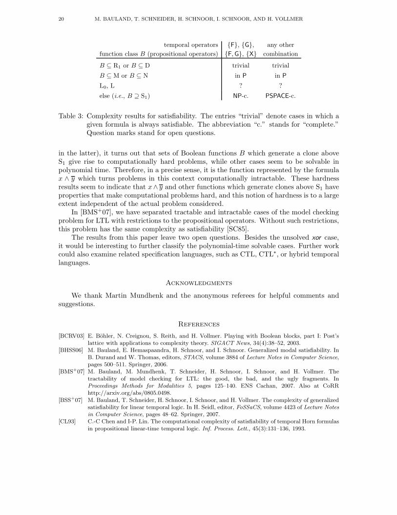
temporal operators {F}, {G}, any other

function class B (propositional operators) {F,G}, {X} combination

B ⊆ R1 or B ⊆ D trivial trivial

B ⊆ M or B ⊆ N in P in P

L0, L ? ?

else (i.e., B ⊇ S1) NP-c. PSPACE-c.

Table 3: Complexity results for satisfiability. The entries “trivial” denote cases in which agiven formula is always satisfiable. The abbreviation “c.” stands for “complete.”Question marks stand for open questions.

in the latter), it turns out that sets of Boolean functions B which generate a clone aboveS1 give rise to computationally hard problems, while other cases seem to be solvable inpolynomial time. Therefore, in a precise sense, it is the function represented by the formulax ∧ y which turns problems in this context computationally intractable. These hardnessresults seem to indicate that x∧ y and other functions which generate clones above S1 haveproperties that make computational problems hard, and this notion of hardness is to a largeextent independent of the actual problem considered.

In [BMS+07], we have separated tractable and intractable cases of the model checkingproblem for LTL with restrictions to the propositional operators. Without such restrictions,this problem has the same complexity as satisfiability [SC85].

The results from this paper leave two open questions. Besides the unsolved xor case,it would be interesting to further classify the polynomial-time solvable cases. Further workcould also examine related specification languages, such as CTL, CTL∗, or hybrid temporallanguages.

Acknowledgments

We thank Martin Mundhenk and the anonymous referees for helpful comments andsuggestions.

References

[BCRV03] E. Bohler, N. Creignou, S. Reith, and H. Vollmer. Playing with Boolean blocks, part I: Post’slattice with applications to complexity theory. SIGACT News, 34(4):38–52, 2003.

[BHSS06] M. Bauland, E. Hemaspaandra, H. Schnoor, and I. Schnoor. Generalized modal satisfiability. InB. Durand and W. Thomas, editors, STACS, volume 3884 of Lecture Notes in Computer Science,pages 500–511. Springer, 2006.

[BMS+07] M. Bauland, M. Mundhenk, T. Schneider, H. Schnoor, I. Schnoor, and H. Vollmer. Thetractability of model checking for LTL: the good, the bad, and the ugly fragments. InProceedings Methods for Modalities 5, pages 125–140. ENS Cachan, 2007. Also at CoRRhttp://arxiv.org/abs/0805.0498.

[BSS+07] M. Bauland, T. Schneider, H. Schnoor, I. Schnoor, and H. Vollmer. The complexity of generalizedsatisfiability for linear temporal logic. In H. Seidl, editor, FoSSaCS, volume 4423 of Lecture Notesin Computer Science, pages 48–62. Springer, 2007.

[CL93] C.-C Chen and I-P. Lin. The computational complexity of satisfiability of temporal Horn formulasin propositional linear-time temporal logic. Inf. Process. Lett., 45(3):131–136, 1993.


[Coo71] S. A. Cook. The complexity of theorem proving procedures. In Proceedings 3rd Symposium onTheory of Computing, pages 151–158. ACM Press, 1971.

[Dal00] V. Dalmau. Computational Complexity of Problems over Generalized Formulas. PhD thesis, De-partment de Llenguatges i Sistemes Informatica, Universitat Politecnica de Catalunya, 2000.

[DFR00] C. Dixon, M. Fisher, and M. Reynolds. Execution and proof in a Horn-clause temporal logic.In H. Barringer, M. Fisher, D. Gabbay, and G. Gough, editors, Advances in Temporal Logic,volume 16 of Applied Logic Series, pages 413–433. Kluwer, 2000.

[DS02] S. Demri and P. Schnoebelen. The complexity of propositional linear temporal logics in simplecases. Inf. Comput., 174(1):84–103, 2002.

[EES90] E. A. Emerson, M. Evangelist, and J. Srinivasan. On the limits of efficient temporal decidability.In LICS, pages 464–475. IEEE Computer Society, 1990.

[Hal95] J. Y. Halpern. The effect of bounding the number of primitive propositions and the depth ofnesting on the complexity of modal logic. Artif. Intell., 75(2):361–372, 1995.

[Hem01] E. Hemaspaandra. The complexity of poor man’s logic. J. Log. Comput., 11(4):609–622, 2001.[Lew79] H. Lewis. Satisfiability problems for propositional calculi. Mathematical Systems Theory, 13:45–

53, 1979.[Low08] G. Lowe. Specification of communicating processes: temporal logic versus refusals-based refine-

ment. Formal Aspects of Computing, 20(3):277–294, 2008.[Mar04] N. Markey. Past is for free: on the complexity of verifying linear temporal properties with past.

Acta Informatica, 40(6-7):431–458, 2004.[Nor05] G. Nordh. A trichotomy in the complexity of propositional circumscription. In Proceedings of

the 11th International Conference on Logic for Programming, volume 3452 of Lecture Notes inComputer Science, pages 257–269. Springer Verlag, 2005.

[Pip97] N. Pippenger. Theories of Computability. Cambridge University Press, Cambridge, 1997.[Pnu77] A. Pnueli. The temporal logic of programs. In FOCS, pages 46–57. IEEE, 1977.[Pos41] E. Post. The two-valued iterative systems of mathematical logic. Annals of Mathematical Studies,

5:1–122, 1941.[Rei01] S. Reith. Generalized Satisfiability Problems. PhD thesis, Fachbereich Mathematik und Infor-

matik, Universitat Wurzburg, 2001.[RV03] S. Reith and H. Vollmer. Optimal satisfiability for propositional calculi and constraint satisfaction

problems. Information and Computation, 186(1):1–19, 2003.[RW05] S. Reith and K. W. Wagner. The complexity of problems defined by Boolean circuits. In Proceed-

ings International Conference Mathematical Foundation of Informatics, (MFI99); World SciencePublishing, 2005.

[SC85] A. Sistla and E. Clarke. The complexity of propositional linear temporal logics. Journal of theACM, 32(3):733–749, 1985.

[Sch05] H. Schnoor. The complexity of the Boolean formula value problem. Technical report, TheoreticalComputer Science, University of Hannover, 2005.

[Sto77] L. Stockmeyer. The polynomial-time hierarchy. Theoretical Computer Science, 3:1–22, 1977.

This work is licensed under the Creative Commons Attribution-NoDerivs License. To viewa copy of this license, visit http://creativecommons.org/licenses/by-nd/2.0/ or send aletter to Creative Commons, 559 Nathan Abbott Way, Stanford, California 94305, USA.

Documents

The Complexity of Generalized Satisfiability for Linear Temporal Logic