The development and experimental validation of a numerical model of an induction skull melting furnace

The Development and Experimental Validationof a Numerical Model of an Induction Skull Melting Furnace

V. BOJAREVICS, R.A. HARDING, K. PERICLEOUS, and M. WICKINS

Induction skull melting (ISM) is a widely used process for melting certain alloys that are very reactivein the molten condition, such as those based on Ti, TiAl, and Zr, prior to casting components suchas turbine blades, engine valves, turbocharger rotors, and medical prostheses. A major research pro-ject has been undertaken with the specific target of developing improved techniques for casting TiAlcomponents. The aims include increasing the superheat in the molten metal to allow thin section com-ponents to be cast, improving the quality of the cast components and increasing the energy effi-ciency of the process. As part of this, the University of Greenwich (United Kingdom) has developeda dynamic, spectral-method-based computer model of the ISM process in close collaboration with theUniversity of Birmingham (United Kingdom), where extensive melting trials have been undertaken.This article describes in detail the numerical model that encompasses the coupled influences of tur-bulent flow, heat transfer with phase change, and AC and DC magneto-hydrodynamics (MHD) in atime-varying liquid metal envelope. Associated experimental measurements on Al, Ni, and TiAl alloyshave been used to obtain data to validate the model. Measured data include the true root-mean-square (RMS) current applied to the induction coil, the heat transfer from the molten metal to thecrucible cooling water, and the shape of the semi-levitated molten metal. Examples are given of theuse of the model in optimizing the design of ISM furnaces by investigating the effects of geometricand operational parameter changes.

I. INTRODUCTION

AS the result of an extensive worldwide research effortto develop gamma-titanium-aluminide (�-TiAl) alloys forhigh-performance components, the small-scale productionof certain components such as turbine blades, exhaust valves,and turbocharger rotors has started.[1,2] However, there arevarious technological and economic barriers to more wide-spread production and there is a particular need to developrobust foundry techniques suitable for the high-volume pro-duction of (near)-net-shape components.

The induction skull melting (ISM) process is currentlythe most effective means of melting these alloys, which arethen usually investment cast into ceramic shell molds. Melt-ing is carried out in a water-cooled copper crucible with thepower supplied by a high-intensity induction field (Figure 1).In early furnace designs, the first metal to melt immediatelyresolidified on the inner wall of the crucible to form a “skull,”which acted as a protective container for the remainder ofthe melt. However, the energy efficiency of such furnaceswas poor and the superheat was typically �10 °C to 20 °Cwhen melting Ti alloys. The low superheat made it difficultto fill thin section castings unless rapid pouring was used,but this led to various casting problems, particularly entrainedbubble defects. In the latest generation of furnaces, changesto the crucible design and power supply allow more powerto be supplied to the metal without it becoming unstable,

which enables it to be pushed away from the side wall. Asa result, the superheat has been increased to �33 °C to 62 °C,depending on the melting atmosphere used.[3,4]

A major project in the United Kingdom has involved closecollaboration between practical melting and casting researchat the University of Birmingham[4] and the development ofa comprehensive computer model of an ISM furnace at theUniversity of Greenwich,[5,6] with the aims of increasing thesuperheat available and improving the quality of �-TiAlinvestment castings. This article describes the mathematicalbasis of the model, the trials undertaken to validate it, andsome examples of where the model has either enhanced theunderstanding of the process or provided suggestions forfuture equipment development.

II. THE COMPUTER MODEL OF THE ISMPROCESS

A. Introduction

An essential part of the ISM furnace is the water-cooledcopper crucible used to contain the metal charge, which isthen melted by the induced currents generated by an exter-nal high-frequency AC coil. The copper wall is made of elec-trically insulated segments (or “fingers”) so that the magneticfield can effectively penetrate through it via the develop-ment of high-density AC current loops within the individualsegments. The induced currents heat and melt the metal charge,which ideally should not be in contact with the crucible walls.These induced currents incur relatively high energy losses,which are removed as heat by the cooling liquid circulatingin the copper segments. In addition to these direct Joule losses,there are diffusive and convective heat losses from the metalcharge where it is in contact with the crucible walls and base,and relatively smaller radiation losses from the molten metal

METALLURGICAL AND MATERIALS TRANSACTIONS B VOLUME 35B, AUGUST 2004—785

V. BOJAREVICS, Senior Research Fellow, and K. PERICLEOUS, Pro-fessor, are with the School of Computing and Mathematics, University ofGreenwich, London SE10 9LS, United Kingdom. Contact e-mail: [email protected] R.A. HARDING, Senior Research Fellow, and M. WICKINS,Research Fellow, are with the IRC in Materials Processing, The Universityof Birmingham, Birmingham B15 2TT, United Kingdom.

Manuscript submitted September 19, 2003.

19-E-TP-03-20B-N.qxd 1/1/04 10:28 PM Page 785

surface. In the case of TiAl alloys, temperatures in excess of�1550 °C are necessary to melt the metal, and a superheatof at least 100 °C would be desirable for casting thin sectioncomponents such as near-net-shape turbine blades. In a deli-cate balance among the induced electromagnetic force, thefluid pressure, inertial forces, and gravity, the molten metalis held away from the wall, minimizing contact with the water-cooled fingers. This critical feature affects the efficiency ofthe process. Contact with the wall is undesirable because itproduces a thermal path from the metal to the cooling water,and can also lead to an intermittent electrical “short-circuit”of the crucible segments. The shape and position of the liq-uid metal depend on the instantaneous balance of forces act-ing on it. Hence, the electromagnetic field and the associatedforce field are strongly coupled to the free-surface dynamicsof the liquid metal, the turbulent fluid flow within it, and theheat transfer. This dynamic coupling of fields that is tradi-tionally solved using different numerical methods poses a con-siderable modeling challenge, which has been addressed hereusing a unique spectral-collocation approach.

Historically, this complex problem has been studied exten-sively both experimentally[7–11] and numerically.[11–16] Earlynumerical simulation efforts mostly concentrated on the elec-trodynamic part of the problem;[12,13,14] heat transfer wastreated as a stationary problem; the liquid metal shape wasobtained from a magnetostatic approximation; and the tur-bulence of the melt velocity field was considered within therange of stationary k-�-type models.[14,16] The present workwas carried out under the concept of the multiphysics com-mon modeling environment.[17] The first step toward the ISMmodel concerned the simulation of a semi-levitation melt-ing device,[18] where the time-dependent coupling betweenthe electromagnetic field and the melt free-surface changeduring the melting process was studied in the absence ofsidewalls. The importance of turbulence and its time devel-opment in the confines of the melt envelope was highlightedand appropriate turbulence models selected[19] and validatedagainst detailed measurements in a liquid metal (In-Ga-Sn)experiment conducted at room temperature.[20]

The numerical model presented in this article uses anaxisymmetric pseudo-spectral representation of the equations

solved, but it also relies on other, auxiliary models (finite-volume and integral equation) to represent particular detailsof the problem.

The results presented will compare the predicted temper-ature history of the melting process with experimentally meas-ured data. The heat losses in the various parts of the furnacewill be analyzed and compared with measurements. The free-surface observations and height measurements will be com-pared with the numerically predicted surface shapes. Withthe aid of detailed flow and temperature fields, the numeri-cal simulations provide explanations for both the thermalefficiency loss at various stages of melting and the result-ing limited superheat of the melt. The numerical model isa versatile tool for assessing the effect of process variations,optimizing the process of achieving higher melt superheatand increased stability of the melt confinement, and for find-ing ways to save energy. This article will discuss just someof the large number of simulations conducted.

The dynamic simulation has given new insights into thevarious factors affecting the process. This is shown in resultsthat demonstrate the effect of changes in the melt weight,AC current frequency, and induction coil position, as wellas the effects of turbulence damping on heat losses achievedusing an additional, external DC electromagnetic field.

B. Description of the Numerical Models Used

The mathematical basis of the present model is the time-dependent Navier-Stokes and continuity equations for anincompressible fluid, and the thermal energy conservationequations for the fluid and solid zones of the metal charge:

[1]

[2]

[3]

where v is the velocity vector; p the pressure; � the density;ve the effective viscosity, variable in time and position andgiven by ve � vT � v, where vT and v are turbulent and lam-inar viscosities, respectively; f the local (AC-cycle-averaged)electromagnetic force; KD the Darcy resistance term repre-senting the mushy zone; and g the gravity vector. The tur-bulent viscosity is the subject of the turbulence model givenin a later section. In Eq. [3], T is the temperature; �e ��T � � the effective thermal diffusivity; Cp the specificheat; Cp* the solid fraction-modified specific heat functionthat accounts for latent heat effects (Reference 18 containsthe details), and J2/� the Joule heating term (J is the electriccurrent density and � the electrical conductivity).

The numerical solution of the coupled Eqs. [1] through [3]by the pseudo-spectral collocation method, employing thecontinuous coordinate transformation for the shape track-ing, is described in detail in a previous publication[18]

concerning the closely related problem of the semi-levitationmelting of liquid metals. The main solution steps andprocedures are listed; the full description is in the refer-ence.[18] The time-dependent fluid flow problem is closedwith appropriate accurate boundary conditions: at the free-surface of the liquid metal, the normal hydrodynamic stressis compensated by the surface tension, while the tangential

C*p (tT � v # §T) � § # (Cpae§T ) � r1 | J |2/s

§ # v � 0

� § # (ve (§v � §vT)) � g

tv � (v # §)v � r1(§p � f) KDv

786—VOLUME 35B, AUGUST 2004 METALLURGICAL AND MATERIALS TRANSACTIONS B

Fig. 1—Schematic part view of a water-cooled segmented crucible usedfor ISM.

19-E-TP-03-20B-N.qxd 1/1/04 10:28 PM Page 786

stress is zero. To ensure mass conservation, a kinematic condi-tion ensures that the free-surface location moves with thefluid material particles. The mathematical formulation andthe numerical implementation are given in a previous pub-lication.[18] The no-slip condition is applied to the velocityat solid walls wherever there is contact at any given time.The free-surface contact position moves as determined bythe force balance and the kinematic conditions. The chang-ing shape of the liquid metal envelope is represented inthe spectral-collocation mesh using coordinate transforma-tions from an initially spherical mesh. During melting, thesolid-liquid interface is traced automatically as the solidustemperature surface T � TS moves with the coupled effectsof the solid-fraction-modified specific heat function C*p.Details of the full coordinate representations of Eq. [1]through [3] and the boundary conditions have been describedelsewhere.[18]

The temperature boundary conditions are expressed bythe thermal flux (heat losses) to the surroundings by radiationand the effective turbulent heat transfer. At solid walls, thetemperature boundary condition is expressed by an effectiveconvective heat transfer expression, quantified with an empiri-cal heat transfer coefficient Hch(T):

[4]

where Tw is the wall temperature (in this case fixed to theaverage temperature of the cooling liquid inside the copperwall). The data for Hch(T) [Wm2K1] were obtained fromcomparisons with the experimentally measured heat lossesat the water-cooled walls, as will be described subsequently.It has been found that the final results are not very sensitiveto small changes in the heat transfer coefficient value. Theheat transfer coefficient in the present model depends on themetal temperature T at the wall contact position:

[5]

where TS is the metal solidus temperature. At the free sur-face the radiation condition is used:

[6]

where the value of the emissivity � was set to 0.3 accordingto available data[3,21] and �B is the Stefan-Boltzmann constant.

The temperature boundary conditions depend on the localeffective thermal diffusion coefficient �e at the wall and thefree surface, which is proportional to the effective turbulentviscosity ve determined from the numerical turbulence model.Therefore, the turbulence model has a direct influence onthe thermal fluxes at the walls. The two-equation k-�model[19] resolves the flow from laminar to developed tur-bulent states, and therefore can be considered suitable forthe flow within the slowly moving mushy zones during thephase change steps and, at the same time, for the bulk of thefully molten metal at the final mixing stages. The � variableis related to the reciprocal turbulent time scale (frequencyof vorticity fluctuations) and the k variable is the turbulencekinetic energy per unit mass. The k-� equations are:

[7]tv � v # §v � § # [(v � sv vT)§v] � a vk G b v2

tk � v # §k � § # [(v � sk vT)§k] � G b* v k

rCp ae n T � �sB (T4 Tw

4)

� (T TS)*200, if T � TS

Hch � 150, if T TS, and Hch � 150

rCp ae n T � Hch (T) # (T Tw)

where G is the turbulent kinetic energy generation term, a func-tion of the mean velocity strain rate �. Different model con-stants and “wall damping” functions in Eq. [7] are defined as:

a, a*, �, �*––functions depending on [8]

The full expressions for the functions can be found elsewhere.[19,20] The solution is sought with the boundary conditions:

[9]

[10]

where R0 is a typical scale of the problem and was definedas the crucible radius. In the present work, the k-� modelhas been applied within the pseudo-spectral framework.[18,20]

The computation follows in detail the time development ofthe turbulent characteristics determined by the coupled non-linear transport equations accounting for a continuous gen-eration and destruction of the turbulent energy. It is necessaryto emphasize here that the turbulence model in Eqs. [7]through [10] is not specifically modified for the magneto-hydrodynamic MHD application. Numerical tests against theliquid In-Ga experiment,[20] involving the direct mean andfluctuating velocity measurements, showed that the modelis capable of adjusting automatically to the electromagnetic-force-generated mean-velocity field changes in time andspace, and the generation term G in Eq. [7] is sufficient asthe only link to the changing velocity field. The settingsfor the boundary conditions in Eqs. [9] through [10] and themodel constants and functions in Eq. [8] used in this workare the same as were used in the experiment.[20] As mentionedpreviously, the mushy-zone modeling includes the turbulentflow, and the Darcy term in Eq. [1] is responsible for theflow damping in this zone[18] and even for the motionlesssolid-metal zone during the melting phase. Therefore, theturbulence model boundary conditions are shown in Eqs. [9]and [10] at the external fluid boundary, and there is no needfor additional conditions at the melt boundary.

The axisymmetric approximation is used for the Navier–Stokes and the heat transfer Eqs. [1] through [3], and alsofor the k-� model equations. This allows a solution of themathematical problem in a reasonable total computationaltime. The calculation requires a large number of implicit timesteps with iterative linearization of the nonlinear terms in theequations at each step. The pseudo-spectral spatial repre-sentation is applied to solve the set of nonlinear, variablecoefficient equations for the transformed Navier–Stokes, heat-transfer, and k-� model equations. For the time-dependentsolution, the implicit Euler scheme is used:

[11]

[12]§ # v k � 0

� § # (vek1 1§v k � (§v k)T 2 � r1f k1

v k v k1

�t� (v k1/2 # §)vk1/2 � r1§pk KDv k

at the free surface n k � 0, n v � 0

at solid walls k � 0, v �6v

b(0.1R0)2

RT �k

v # v

sk �1

2 sv �

1

2

vT � a* kv G � 2vT (�:�) � �

1

2(§v � §vT)


19-E-TP-03-20B-N.qxd 1/1/04 10:28 PM Page 787

This ensures sufficient stability for long-term flow calcula-tions. Typically, two or three iterations are necessary for thenonlinear terms at each time step to reach convergence,satisfying the relative maximum error of less than 0.001for the velocity components. Occasionally, the time step isreduced when the iterations do not converge, and increasedback when the convergence improves. The procedure is stablefor the cases presented if the time steps are dynamicallyadjusted according to the iterative loop convergence rate(typically �t � 0.1 to 4.0 ms). Small time steps are requiredto resolve accurately the liquid metal surface change and toensure that the volume conservation has a relative error ofless than 0.001. This condition serves as an additional testfor long-term solution accuracy. The equations for the tem-perature (Eq. [3]) and the turbulence model (Eq. [7]) aresolved in the same manner, using the coordinate transform-ation and similar spectral representation.

Since the electromagnetic force distribution is highly sen-sitive to the shape of the liquid-metal free surface and thematerial properties change with temperature, the former isby necessity recalculated at each time step. The computa-tional procedure for the electromagnetic field is implementedon the same grid as the fluid dynamic equations. The gridensures a high resolution within the skin layer region, usinga Chebyshev polynomial Gauss-Lobatto discretization, whichbecomes exponentially dense at the surface. The electro-magnetic force F is computed using an integral-equation-based algorithm (previously tested in References 18 and 20),which achieves the best compromise between accuracy andspeed of computation. The full coupling of the electromagneticfield with the fluid flow in the time-dependent fluid envelopecan be achieved on the limited size grid used in this work.

A three-dimensional finite volume code is used to computethe electric current distribution within the segmented copperwall fingers. For this purpose, the general multiphysics codePHYSICA[17] was adapted for the sinusoidal electric currentsolution. The computed results[5] showed that the radial elec-tric currents along the gap between adjoining fingers are inopposite directions and are equal in magnitude; therefore, a“quasi-axisymmetric” approximation can be constructed whencomputing the magnetic field outside of their volume andproduced by currents within the fingers.[5] This allows for afast axisymmetric integral equation algorithm to be built,where the effective current path within the fingers is updatedas an axisymmetric average from the three-dimensional finitevolume solution, i.e., located within the external and inter-nal skin layers only, where the skin layer depth is modifiedto account for the radial current dissipation losses.[5,12,13] Thedetails of this procedure are particularly important when deter-mining the Joule heat directly released inside the copperfingers, which is a significant part of the total energy losseswithin the cold crucible.

Where a combination of high-frequency AC and DC mag-netic fields is used, it is also necessary to obtain the time aver-age for the force over the very small field oscillation period(103 to 104 seconds). The electric current in the axisym-metric case is given by Ohm’s law for a moving medium:

[13]

where � is the electrical conductivity and A is the vector poten-tial related to the magnetic field B � curl A. Equation [13]

J � s(t A � v � B) � JAC � Jv

shows that part of the current, JAC, is induced in the conduct-ing medium even in the absence of velocity. It is computedaccording to the mutual inductance algorithm with ellipticintegrals described in detail previously[18] and tested againstanalytical solutions and experimental measurements in moltenIn-Ga-Sn.[20] A similar elliptic integral representation can beused to calculate the DC magnetic field created by an addi-tional external coil. The solution in the liquid volume dependson its free-surface shape and needs to be recomputed whenthe shape changes. The resulting electromagnetic force f, timeaveraged over the AC period in a manner similar to Eq. [13],can be decomposed in two parts:

[14]

where the second, fluid-velocity-dependent part of the forcefv has the following components in the spherical coordinates:

[15]

where the notation x� means the time averaging of x overthe AC period. The magnetic field BR and B� componentsin the expressions in Eq. [15] include AC and DC parts,both of which can produce the time-averaged contributionto the force. It is worthy of note that, even if there is onlythe AC field present, there is, in principle, an averaged fv

contribution to the interaction with the velocity field.

III. DATA FOR VALIDATION OF THECOMPUTER MODEL

A. Thermo-Physical Data

The computer model requires accurate thermophysical andelectrical properties of all the materials present. In commonwith solidification modeling, the modeling of a melting fur-nace needs such data in both the solid and liquid states. BothTi and TiAl alloys are very reactive in the molten condi-tion, thus making it difficult to hold them in a refractorycontainer to enable measurements to be made. Various tech-niques, including levitation-melting and pulse-heating(exploding wire) methods have been used in a collaborativeapproach between various European institutes, resulting ina set of values for the Ti-44Al-8Nb-1 B alloy of particularinterest.[21,22]

B. Operational Data

Additional operational data were required both for valida-ting the model and as inputs to it. These included the truecurrent in the induction coil, the temperature during melting,the heat flow to the crucible coolant, and the shape and heightof the molten metal meniscus. The techniques to measurethese data and the typical results are described subsequently.

1. Melting furnaceAll measurements were made at the University of

Birmingham using an ISM furnace supplied by Consarc Engin-eering Ltd. The crucible had a nominal melting capacity of�4.5 kg TiAl and was located inside a chamber to allow melt-ing to be carried out under vacuum or a partial pressure ofargon (Figure 2). The induction coil was connected to a Vari-able Induction Power (VIP) power supply from Inductotherm

fvu � s(u BRBu� v B2R�)

fvR � s(u B2u� v BRBu�)

f � fAC � fv


19-E-TP-03-20B-N.qxd 1/1/04 10:28 PM Page 788

Europe Ltd. providing nominally 350 kW at �7 kHz. Meltingusually involved selecting progressively higher powers withtime. When melting TiAl or Ni alloys, 50 kW was appliedinitially and the power then increased in 50 kW steps to200 kW to achieve melting, and then to 350 kW for a shorttime to maximize superheat in the metal charge without over-heating the recirculating cooling water. The maximum powerwas usually limited to 200 kW when melting Al alloys.

The melting trials were carried out using a variety ofmaterials:

1. pure (99.99 pct) aluminum,2. a wrought-aluminum alloy (grade 6082T6 to BS1474)

containing 0.89 pct Si, 0.23 pct Fe, 0.043 pct Cu, 0.71 pctMn, 0.88 pct Mg, 0.14 pct Cr, 0.03 pct Zn, 0.014 pct Ti,and the balance Al,

3. a nickel alloy (Rolls-Royce-grade MSRR 7047, equivalentto IN100) of the following specification: 8 to 11 pct Cr,4.5 to 5 pct Ti, 5 to 6 pct Al, 13 to 17 pct Co, 2 to 4 pctMo, and 0.7 to 1.2 pct V, and

4. a Ti-45Al-8Nb-1B (at. pct) alloy, produced as continu-ously cast billets in the IRC’s plasma melting furnace,and used for most TiAl melts. The TiAl returns were usedfor some melts.

2. Induction coil current calibrationThe VIP power supply provided constant power output (for

a given selected value), but the instrumentation showed onlythe nominal melting power (in kW) and not the current in thecoil, which was an essential input into the model. The powersupply was connected to the coil via busbars, flexible leads,and a coaxial port to feed the power through the wall of thevacuum vessel, to allow the crucible to be tilted. The currentwas measured outside the vacuum chamber using a currenttransformer (CT) placed around one pair of the flexible leadsof the same polarity. The CT was designed for frequencies upto 10 kHz and had a current ratio of 1600:1. A calibrated 1 ohmresistor was connected in parallel with the CT and the voltageacross it was measured with an oscilloscope. The resistor wasmounted on a water-cooled copper heat sink to prevent over-heating. The RMS coil current I in amperes was then given by:

[16]I � 1600 V/(2R1 2 )

where V is the peak-to-trough voltage and R the actual valueof the resistance at this frequency. The operating frequencywas also measured using the oscilloscope. Attempts to mea-sure the true power supplied to the coil were unsuccessfuldue to the difficulty of accurately measuring the phase angleat the relatively high frequency (�7 kHz) used.

Unless stated otherwise, all melting was done under a par-tial pressure of 20 kPa of argon and the power was rampedup in 50 kW steps (�60 seconds at each) to a maximum of350 kW. Regular readings were taken of the voltage acrossthe CT resistor and the VIP power. Once the maximum powerhad been reached and equilibrium established, the power wasreduced in steps and further readings made. At the lowerpower levels, the metal was barely pushed away from thewalls and started to solidify.

Figure 3 shows the coil current when the various alloyswere melted using this schedule. Melting of the Ni alloystarted at �300 kW; once it was fully molten at 350 kW, thepower was ramped down to zero. The metal remained levi-tated away from the crucible wall until the power reached�100 kW. It can be seen that the coil current was margin-ally lower during heating up, i.e., when the charge was stillsolid. Melts carried out with the TiAl alloy and the sameschedule showed similar results: Figure 3 shows that the coilcurrent was again lower during heating up, although therewas a change of slope at �250 kW and the “increasingpower” data became coincident with the “decreasing power”data. This occurred at the same time as the charge becamefully molten. Repeat melts showed a similar behavior. Forthe Al alloy, a point was obtained at 350 kW by applyingfull power for �40 seconds and completing the measurementjust as the corners of the billet began to melt. The power wasthen turned off to allow the billet to resolidify. The powerwas subsequently ramped up in �50-kW steps, but the max-imum power was restricted to 200 kW to avoid losing mol-ten alloy by expulsion. The results in Figure 3 show that the


Fig. 2—Vacuum melting chamber containing an ISM furnace.

Fig. 3—ISM coil current calibrations when melting different materials.

19-E-TP-03-20B-N.qxd 1/1/04 10:28 PM Page 789

current was slightly lower in the molten condition, in con-trast to the slightly higher currents found when the Ni andTiAl alloys were molten.

Comparison of the results shows that the calibration curvefor the Al alloy was slightly higher than the others. The find-ing that the material does not have a very significant effecton the coil current calibration was unexpected, since thethree alloys have very different electromagnetic properties.

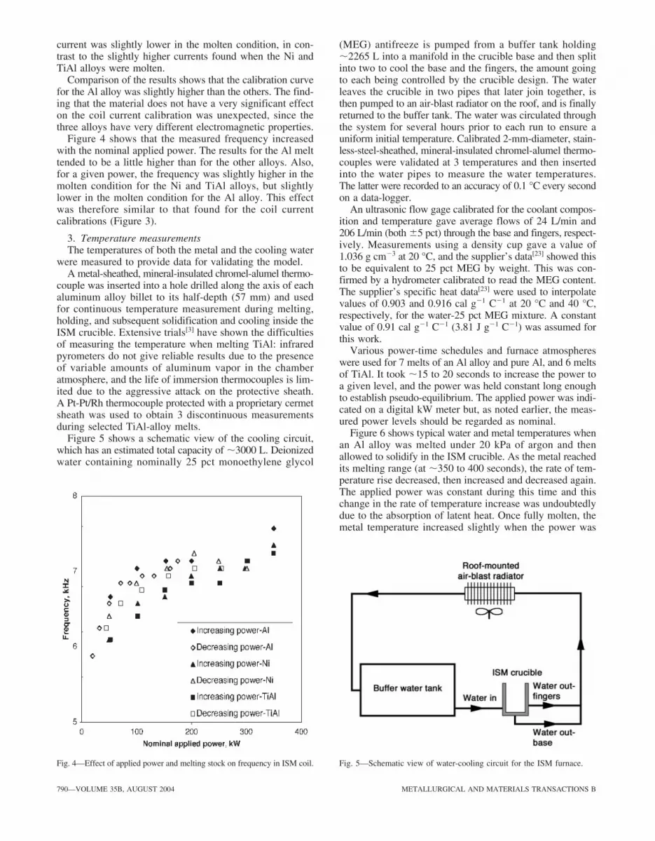
Figure 4 shows that the measured frequency increasedwith the nominal applied power. The results for the Al melttended to be a little higher than for the other alloys. Also,for a given power, the frequency was slightly higher in themolten condition for the Ni and TiAl alloys, but slightlylower in the molten condition for the Al alloy. This effectwas therefore similar to that found for the coil currentcalibrations (Figure 3).

3. Temperature measurementsThe temperatures of both the metal and the cooling water

were measured to provide data for validating the model.A metal-sheathed, mineral-insulated chromel-alumel thermo-

couple was inserted into a hole drilled along the axis of eachaluminum alloy billet to its half-depth (57 mm) and usedfor continuous temperature measurement during melting,holding, and subsequent solidification and cooling inside theISM crucible. Extensive trials[3] have shown the difficultiesof measuring the temperature when melting TiAl: infraredpyrometers do not give reliable results due to the presenceof variable amounts of aluminum vapor in the chamberatmosphere, and the life of immersion thermocouples is lim-ited due to the aggressive attack on the protective sheath.A Pt-Pt/Rh thermocouple protected with a proprietary cermetsheath was used to obtain 3 discontinuous measurementsduring selected TiAl-alloy melts.

Figure 5 shows a schematic view of the cooling circuit,which has an estimated total capacity of �3000 L. Deionizedwater containing nominally 25 pct monoethylene glycol

(MEG) antifreeze is pumped from a buffer tank holding�2265 L into a manifold in the crucible base and then splitinto two to cool the base and the fingers, the amount goingto each being controlled by the crucible design. The waterleaves the crucible in two pipes that later join together, isthen pumped to an air-blast radiator on the roof, and is finallyreturned to the buffer tank. The water was circulated throughthe system for several hours prior to each run to ensure auniform initial temperature. Calibrated 2-mm-diameter, stain-less-steel-sheathed, mineral-insulated chromel-alumel thermo-couples were validated at 3 temperatures and then insertedinto the water pipes to measure the water temperatures.The latter were recorded to an accuracy of 0.1 °C every secondon a data-logger.

An ultrasonic flow gage calibrated for the coolant compos-ition and temperature gave average flows of 24 L/min and206 L/min (both �5 pct) through the base and fingers, respect-ively. Measurements using a density cup gave a value of1.036 g cm3 at 20 °C, and the supplier’s data[23] showed thisto be equivalent to 25 pct MEG by weight. This was con-firmed by a hydrometer calibrated to read the MEG content.The supplier’s specific heat data[23] were used to interpolatevalues of 0.903 and 0.916 cal g1 C1 at 20 °C and 40 °C,respectively, for the water-25 pct MEG mixture. A constantvalue of 0.91 cal g1 C1 (3.81 J g1 C1) was assumed forthis work.

Various power-time schedules and furnace atmosphereswere used for 7 melts of an Al alloy and pure Al, and 6 meltsof TiAl. It took �15 to 20 seconds to increase the power toa given level, and the power was held constant long enoughto establish pseudo-equilibrium. The applied power was indi-cated on a digital kW meter but, as noted earlier, the meas-ured power levels should be regarded as nominal.

Figure 6 shows typical water and metal temperatures whenan Al alloy was melted under 20 kPa of argon and thenallowed to solidify in the ISM crucible. As the metal reachedits melting range (at �350 to 400 seconds), the rate of tem-perature rise decreased, then increased and decreased again.The applied power was constant during this time and thischange in the rate of temperature increase was undoubtedlydue to the absorption of latent heat. Once fully molten, themetal temperature increased slightly when the power was


Fig. 4—Effect of applied power and melting stock on frequency in ISM coil. Fig. 5—Schematic view of water-cooling circuit for the ISM furnace.

19-E-TP-03-20B-N.qxd 1/1/04 10:28 PM Page 790

increased at �535 seconds, and then slowly decreased againduring long-term holding. Increasing the power from 150 to200 kW had no measurable effect on the metal temperature.The inlet water temperature gradually increased throughoutthe melt, and the outlet temperatures from the base and fin-gers increased noticeably whenever the induction power wasincreased. However, after the initial jump, the increase gen-erally became more steady, although there were several dis-continuities in the outlet temperature from the fingers. Sincethe applied power was steady during this period, these fluc-tuations suggest that changes were taking place in the contactbetween the molten metal and the crucible.

Figure 7 shows the water temperatures and applied powerschedule when melting a TiAl billet under 20 kPa of argon.Steps can be seen in the outlet water temperatures that cor-responded closely with the steps in the applied power, withthe exception of some blips in the base water temperaturecurve at �500 to 510 seconds.

The temperature data were used to calculate heat losses intothe coolant as follows: V liters of coolant of density � (g cm3)and specific heat Cp (J g1 C1) pass through the crucible in1 second equal to a mass M � � � 1000 � V (g). During thistime, the coolant temperature increases by �T (°C). The heatQ absorbed by the coolant in 1 second is given by Q � M �Cp � �T. Substituting the values of � and Cp given earlier forthe water-MEG coolant:

[17]

Substituting the measured flow rates for the base and thefingers gives:

[18]

[19]Qfing �13551 # �T (J s1) �13.551 # �T (kW) for the fingers

Qbase � 1579 # �T (J s1) � 1.579 # �T (kW) for the base

Q � r # 1000 # V # Cp# �T � 3947 # V # �T (J s1)

The water temperature changes from all the experimentalruns were converted to heat losses and plotted against time.As an example, the temperature data in Figure 7 are con-verted to heat losses in Figure 8, which also shows the appliedpower. There was a clear increase in the heat loss to the fin-gers and base every time the applied power was increasedand there was a general trend toward a plateau at the end ofeach holding period.

Data such as those in Figure 8 were used to estimate theheat losses to the base and fingers toward the end of each


Fig. 6—Changes in the water and metal temperatures during the ISM of3.6 kg of an Al alloy under 20 kPa of argon and its subsequent in-situsolidification.

Fig. 7—Water temperature changes when ISM 4.6 kg of TiAl alloy under20 kPa of argon.

Fig. 8—Power input and heat losses to ISM crucible base and fingers whenmelting 4.6 kg of a TiAl alloy under 20 kPa of argon.

19-E-TP-03-20B-N.qxd 1/1/04 10:28 PM Page 791

holding period. Figure 9 shows that the majority of pointsfor all the pure Al and Al alloy melts fell onto straight orgently curved lines, even though these melts were carried outunder different conditions (vacuum or 20 or 80 kPa of argon).The results for one melt were somewhat at variance (in thismelt, the maximum power was applied for a very short periodof time to a solid billet, so the results may not be directlycomparable with the others). The results for the TiAl meltsare shown in Figure 10. The results are again remarkably

consistent with all the data falling onto gently curved linesfor the fingers and base. As when melting Al, there was nodiscernible effect of the melting stock (billet or returns) ormelting atmosphere (vacuum or 20 or 80 kPa of argon). Com-parison of Figures 9 and 10 shows that the alloy had verylittle effect on the heat loss to the fingers and base of thecrucible.

The heat losses to the crucible were subtracted from thenominal applied power to give the amount of energy absorbedby the metal (plus the losses in the coil, power leads, etc.)and this was expressed as a percentage of the total appliedpower to give a measure of the efficiency of the furnace.Figure 11 shows a clear decrease in the efficiency withincreasing applied power, and that there is no consistenteffect of the alloy being melted. When the metal is com-pletely molten and its temperature is stable, a thermal bal-ance is established between the input Joule heating and theheat lost to the cooling water; thus, the downward trend inFigure 11 represents the increased losses in the power sup-ply, coaxial port, and power leads as the source powerincreases.

4. Meniscus heightThe progress of melting can be observed through a port

that is almost vertically over the melt. This gives a distortedimpression of the shape of the molten metal (Figure 15 willlater show typical views) and was unsuitable for quantita-tively validating the model.

Instead, the height of the center of the molten-Al alloywas detected by slowly moving a thin thermocouple down-ward until it registered a significant temperature rise as ittouched the surface. The induction power was then reducedto zero so that the metal collapsed into the ISM crucible andsolidified. The vacuum chamber was opened and the posi-tion of the thermocouple tip was measured relative to thetop of the crucible. The measurements made for 3 charge


Fig. 9—Summary of heat loss measurements from ISM fingers and basewhen melting aluminum alloys.

Fig. 10—Summary of heat loss measurements from ISM fingers and basewhen melting TiAl alloys.

Fig. 11—Energy efficiency of ISM furnace when melting Al and TiAlalloys.

19-E-TP-03-20B-N.qxd 1/1/04 10:28 PM Page 792

weights and 2 applied power levels are shown in Figure 12.As would be expected, the meniscus was pushed higher asthe power increased and this effect increased as the chargeweight increased. However, it came as a considerable surpriseto discover that the 2.8-kg melts protruded above the cruciblerim, since this was not at all obvious when viewing the melts.

The temperature of the metal was continuously monitoredduring these melts; Figure 13 shows the changes from theonset of melting. In each case, the temperature rose to a

maximum and then decayed during prolonged holding. Forthe 2 lower melt weights, both the maximum temperatureand the rate of decay increased with increasing melt weightand power. However, for the heaviest charge (2.8 kg), themaximum temperature apparently decreased when the hold-ing power was increased; this is possibly attributable to themetal being levitated above the crucible rim, leading to alack of coupling.

The meniscus height of the Ti-44Al-8Nb-1B alloy wasmeasured by slowly inserting a wire probe into the moltenmetal. This melted back to the meniscus surface and left adroplet of metal on the end, which marked the top and bot-tom positions of the oscillating meniscus. The mean menis-cus height relative to the top of the crucible is shown as afunction of the applied power in Figure 14 for 3 differentmelt weights. As expected, the meniscus height increasedwith increasing melt weight and power. The 4-kg melt pro-truded above the top of the crucible, which can explain theinstability that was sometimes experienced; this undoubt-edly affected the superheat achieved in the melt.

IV. MODELING RESULTS: VALIDATIONAND ISM MODIFICATIONS

A. Predicting the Melt History

For visual clarity, the best experimental results wereobtained for the metals of lower melting temperatures, suchas aluminum in an argon atmosphere, since a clear view ofthe melt surface could be maintained during the whole melt-ing cycle. Figure 15 show the views from the observationport at different stages of the melting cycle for an aluminumalloy.

The numerical simulation results for a complete meltsequence are presented in perspective, cut in the vertical


Fig. 12—Measured height of the meniscus when melting an Al alloy in anISM furnace.

Fig. 13—Temperature changes in Al alloy billets of different weights whenmelted in an ISM furnace under 20 kPa of argon with two input powerlevels.

Fig. 14—Measured height of the meniscus when melting a TiAl alloy inan ISM furnace.

19-E-TP-03-20B-N.qxd 1/1/04 10:28 PM Page 793

mid-section, in Figures 15(a) through (d). Qualitatively,the simulation convincingly mirrors the experimental results.The plots, which are composites of temperature contoursand velocity vectors, show the history of the melt and soafford insight into the process. In the experiments, the currentin the induction coil was increased gradually in steps, andthe calibration curve (Figure 3) was used to provide thecurrent magnitude for input into the numerical simulation,which then shows the following sequence of events.

Melting starts on the cylindrical surface of the ingotadjacent to the coil. The temperature is highest in the surface

skin where the induction current is also largest; from there,the heat slowly penetrates the cylindrical charge in the radialdirection (Figure 15(a), at t � 408 s). The hydrodynamiccomputation begins once a thin layer of liquid is formed.Gravity then drives the flow downward, while the electro-magnetic forces (Figure 17(a)) push the fluid radially inwardto confine and partially oppose its downward motion.

At t � 435 s, the melt reaches and fills the bottom gapbetween ingot and crucible (Figure 15(b)). After the initialstage, when the bottom is filled, the largest Joule heatingconcentration is shifted to the bottom part of the side skin


(a) (b)

Fig. 15—Progress of melting as viewed from above the ISM crucible and the corresponding numerical simulation results in perspective view for the melt-ing sequence of 2.8 kg of Al alloy in the ISM furnace: (a) t � 408 s, I � 4000 A: the first signs of melting appear at the edge (the solid zone is shownin black); (b) t � 435 s, I � 4900 A: the side part is molten and fills in the bottom corner; (c) t � 525 s, I � 4900 A: some metal is still solid at the bot-tom; and (d) t � 838 s, I � 5560 A: melting is complete and the melt top protrudes above the crucible rim.

19-E-TP-03-20B-N.qxd 1/1/04 10:28 PM Page 794

layer, which now lies closer to the source coil and to theinduced electric currents in the segmented wall (Figure 17(b)).

Subsequently, the melting front progresses slowly radi-ally inward (Figure 15(c)). The heat-conduction coefficientwithin the solid part is small compared to the turbulent flowregion, and the phase change from solid to liquid consumessignificant energy, resulting in the slow progress. So, theelectric current and the heating are induced in the side skin-layer, from which convection and gradually intensifying tur-bulent mixing distribute the heat. The water-cooled bottomis always in contact with the metal in this crucible designand takes away heat at a constant rate. This rate increases

when the side gap at the bottom is filled. When the metalmelts close to the bottom, the heat losses increase due toconvection and a quasi-steady-state situation is established,which is disturbed by the final current increase to 5560 A.This results in an increase in the flow intensity and in thelevel of turbulence.

The melt finally acquires a characteristic dome shape,which has also been predicted using the magnetostaticapproach,[10] with the flow dominated by a strong toroidalvortex. The top of the liquid metal protrudes out of the cru-cible in this case (Figure 15(d)). The temperature increaseis very small (672 °C to 690 °C), in spite of the significant


(c) (d )

Fig. 15—(Continued). Progress of melting as viewed from above the ISM crucible and the corresponding numerical simulation results in perspective viewfor the melting sequence of 2.8 kg of Al alloy in the ISM furnace: (a) t � 408 s, I � 4000 A: the first signs of melting appear at the edge (the solid zoneis shown in black); (b) t � 435 s, I � 4900 A: the side part is molten and fills in the bottom corner; (c) t � 525 s, I � 4900 A: some metal is still solidat the bottom; and (d) t � 838 s, I � 5560 A: melting is complete and the melt top protrudes above the crucible rim.

19-E-TP-03-20B-N.qxd 1/1/04 10:28 PM Page 795


Fig. 16—The results for the collapsing and cooling stages (t � 841 s) ofliquid metal in the ISM furnace (2.8 kg of Al alloy) when the electric cur-rent is switched off abruptly (I � 0) at 840 s.

(a)

(b)

Fig. 17—The numerically calculated electric current density and the timeaverage electromagnetic force in the half cross section in the cylindricalcoordinates (r, z) when melting Al alloy in the ISM furnace: (a) t � 410 s,I � 4000 A: first signs of melting; and (b) t � 839 s, I � 5560 A: melt-ing is complete.

rise in the input power (150 to 200 kW). This thermal effi-ciency loss will be discussed later.

Finally, at 840 seconds after the start of heating, the powerwas switched off, and the simulation provides an insightinto the collapse and cooling down of the liquid metal (Fig-ure 16). The residual turbulence remains high and the meltcools initially very quickly until the liquidus temperature isapproached. At this stage, the cooling rate becomes muchslower because of the latent heat release with the solidifi-cation at the walls.

B. Dome Height Comparisons

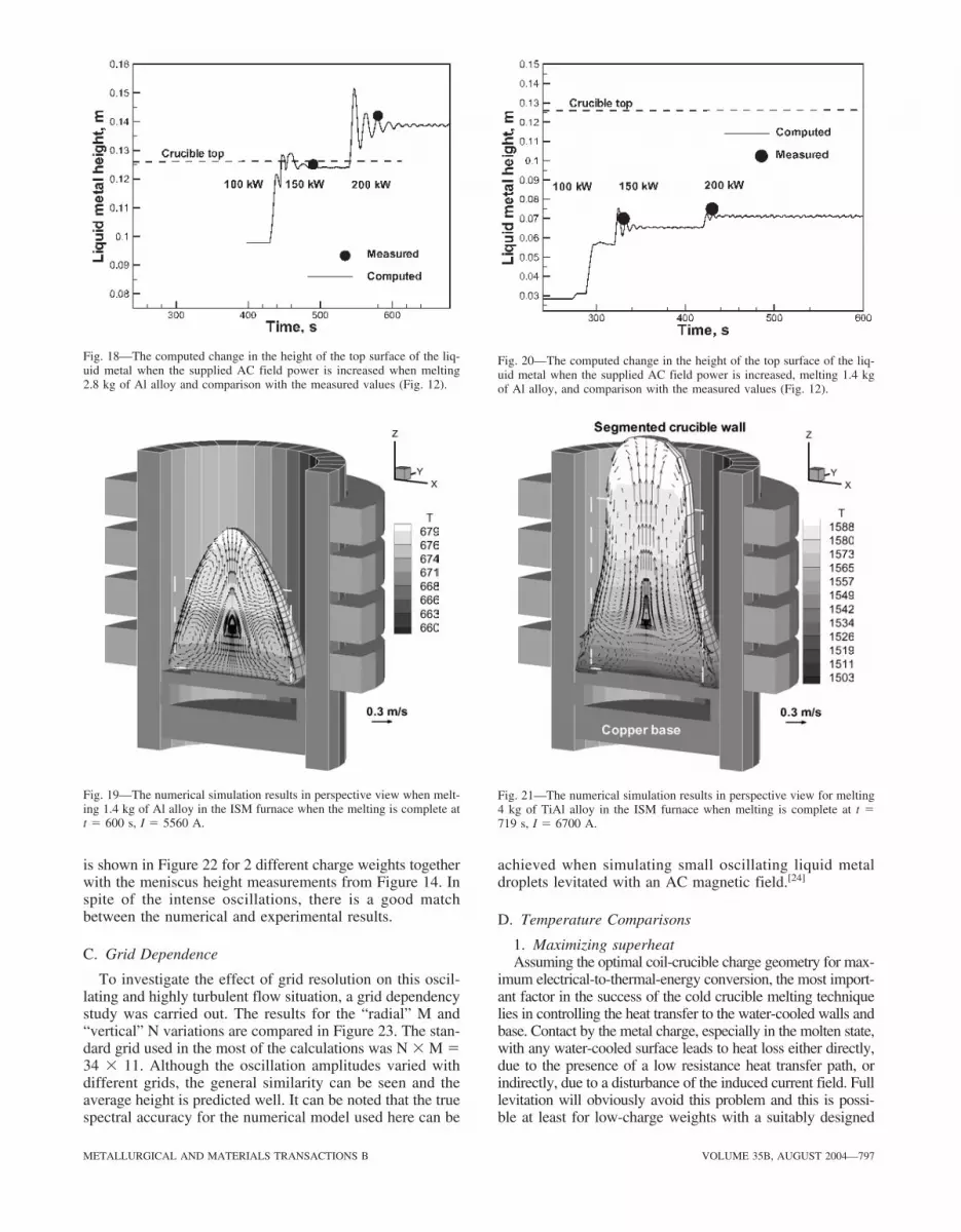
Although the qualitative similarity of the melt shapes inthe simulations and the experimental melts is evident, morequantitative data were necessary to validate the numericalmodel. The experimental data for the liquid metal domeheight are shown in Figure 12 for the Al melts. The numer-ical simulation results in Figure 18 show the oscillatingbehavior of the molten-metal free surface and its dependenceon the electric current magnitude during melting.

The free-surface oscillations were clearly visible in theexperiments as well. The amplitude of the oscillations dependson a variety of factors, such as the relative value of the cur-rent increase step, the shape of the magnetically confinedmetal column prior to the current increase, and the dampingresponse of the turbulent effective viscosity, which dependson the previous history of the flow. Typically the oscillationamplitude decreases when the current is kept constant,although for some cases the oscillation can persist for along time. If the current is abruptly increased by a largeamount, the metal can be physically thrown out of the cru-cible; in the numerical simulation, this is detected as a con-tinuous increase in the metal column height until numericalinstability sets in.

Further tests were carried out by varying the melt weight,as in Figure 12. The corresponding numerical simulation

view for the 1.4-kg charge is shown in Figure 19 for thefinal stage. The bottom confinement for the small load isvery good and there is no contact with the side walls. Thetop oscillations are minimal, as shown in Figure 20, and theaverage heights for the given input powers agree well withthe experimental measurements.

Similar comparisons were made also for the TiAl alloy.The view of the simulated melt at the final stage of the melt-ing is shown in Figure 21. Even with the full power applied,there is contact of the liquid metal with the bottom cornerof the crucible. When the power is abruptly switched off,the metal collapses and the superheat is lost very quicklybecause of the very high level of turbulence created by theintense flow before and during the collapse. The corres-ponding position of the top of the meniscus during melting

19-E-TP-03-20B-N.qxd 1/1/04 10:28 PM Page 796

is shown in Figure 22 for 2 different charge weights togetherwith the meniscus height measurements from Figure 14. Inspite of the intense oscillations, there is a good matchbetween the numerical and experimental results.

C. Grid Dependence

To investigate the effect of grid resolution on this oscil-lating and highly turbulent flow situation, a grid dependencystudy was carried out. The results for the “radial” M and“vertical” N variations are compared in Figure 23. The stan-dard grid used in the most of the calculations was N � M �34 � 11. Although the oscillation amplitudes varied withdifferent grids, the general similarity can be seen and theaverage height is predicted well. It can be noted that the truespectral accuracy for the numerical model used here can be

achieved when simulating small oscillating liquid metaldroplets levitated with an AC magnetic field.[24]

D. Temperature Comparisons

1. Maximizing superheatAssuming the optimal coil-crucible charge geometry for max-

imum electrical-to-thermal-energy conversion, the most import-ant factor in the success of the cold crucible melting techniquelies in controlling the heat transfer to the water-cooled walls andbase. Contact by the metal charge, especially in the molten state,with any water-cooled surface leads to heat loss either directly,due to the presence of a low resistance heat transfer path, orindirectly, due to a disturbance of the induced current field. Fulllevitation will obviously avoid this problem and this is possi-ble at least for low-charge weights with a suitably designed


Fig. 18—The computed change in the height of the top surface of the liq-uid metal when the supplied AC field power is increased when melting2.8 kg of Al alloy and comparison with the measured values (Fig. 12).

Fig. 19—The numerical simulation results in perspective view when melt-ing 1.4 kg of Al alloy in the ISM furnace when the melting is complete att � 600 s, I � 5560 A.

Fig. 20—The computed change in the height of the top surface of the liq-uid metal when the supplied AC field power is increased, melting 1.4 kgof Al alloy, and comparison with the measured values (Fig. 12).

Fig. 21—The numerical simulation results in perspective view for melting4 kg of TiAl alloy in the ISM furnace when melting is complete at t �719 s, I � 6700 A.

19-E-TP-03-20B-N.qxd 1/1/04 10:28 PM Page 797

bowl-shaped segmented crucible.[7,9] Semi-levitation is an alter-native, where contact is only made through the base; this is notpractical, however, due to the inherent instability of the melt.[18]

For the present convex-dome-shaped bottom design, gains maybe achieved by (a) minimizing contact using an optimal coildesign and frequency or (b) reducing heat losses where contactis inevitable through a reduction in turbulence and damping oflarge-scale free-surface oscillations. To this end, experimentsand numerical simulations were carried out to obtain an under-standing of the temperature changes during the melting processand the heat transfer losses to the walls.

2. Heat transfer coefficient estimatesFor the aluminum melts, a thermocouple was used for

continuously recording the temperature during melting, asdescribed in Section III–B–3. Such measurements wereimpossible for TiAl because of the high reactivity of themelt. However, some measurements were available for thecooling stage.[21] These results for the cooling and the ini-tial heating were used to estimate the heat-transfer coeffi-cient given by Eq. [5] and subsequently used for all thenumerical simulations. The cooling simulation is comparedto the measurements in Figure 24. There is clearly a sig-

nificant temperature gradient along the vertical coordinate(Figures 21 and 16), but the cooling curve agrees closelywith the measurements at the given immersion depth of32 mm. It can be noted that the top (free-surface) tempera-ture is initially slightly lower during the cooling stage, per-haps due to radiation losses. However, the top later becomesthe hottest part when the heat loss to the walls predominates.

3. Temperature history and power distributioncomparisons

The heat losses from both the side wall fingers and thebottom of the crucible were derived from water temperaturemeasurements as described in Section III–B–3. The numer-ical results for an aluminum melt are shown in Figure 25together with the measured temperatures in the middle ofthe billet during melting. This also shows the computed tem-perature at the same position and heat losses to the crucible


Fig. 22—The computed change in the position of the top surface of theliquid metal when the power of the supplied AC field is increased, andcomparison with measurements for loads of 3 and 4 kg of TiAl alloy.

Fig. 23—The effect of the computational grid size on the computed oscil-lations of the liquid metal top surface: 4 kg of TiAl alloy.

Fig. 24—Comparison of the measured and computed temperatures for aTiAl melt during cooling after the supplied AC field power is switched off.

Fig. 25—Comparison of the measured temperature and power losses (dashedlines) with the computed data (continuous lines) when melting Al alloy,showing the effect of stepwise increases in the supplied AC field power(dotted line).

19-E-TP-03-20B-N.qxd 1/1/04 10:29 PM Page 798

walls, composed of the directly released Joule heating withinthe copper wall plus the heat fluxes from the melt:

[20]

The heat loss is controlled by the effective turbulent heattransfer because of the relatively high value of the turbulentthermal diffusion coefficient �e. A thermal balance isachieved soon after the metal is fully molten: the total Jouleheating input to the liquid metal equals the total surface heatloss and the melt temperature reaches a plateau. With thesame electrical power input, there is no further increase ofthe melt temperature (Figure 25). Even an increase in thesupplied power gives very little increase in the liquid metaltemperature. A very similar result was also obtained whenmelting TiAl, as shown in Figure 26. This demonstrates boththe universal behavior for the melt which is independent ofboth the alloy and the overall temperature.

E. Parametric Studies

1. The addition of a damping DC fieldThe numerical simulation of the ISM furnace has facili-

tated a deeper understanding of the energy dynamics of theprocess and has helped in the search for new ways to increaseits efficiency. One of the ideas explored in order to increasemelt superheat is illustrated in Figure 27. An additional coilcarrying a DC current is attached at the bottom of the ISMcrucible. The DC magnetic field created by this current eas-ily penetrates the melt, with the highest field intensity occur-ring at the bottom. The resulting combined electromagneticforce has no time-averaged contribution. However, the rela-tively high DC magnetic field (�0.5 T) directly affects themoving electrically-conducting liquid by damping the flowintensity and reducing the turbulence level within the melt, asdescribed by Eq. [15]. The effect is demonstrated in Figure 28,where the computed temperature maximum increases byabout 40 °C when a DC current of 10-kA magnitude isswitched on abruptly at 600 seconds. A better understanding

QS � �rCp ae§T # ndSn

of this phenomenon can be obtained from the comparisonsgiven in Figures 29 and 30. The former shows the magneticfield in the AC and DC cases: the AC field is concentrated inthe external skin layer (Figure 29(a)), whereas the DC fieldpenetrates deep into the volume of the metal (Figure 29(b)).Figure 30(a) shows high fluid velocities and turbulent kineticenergy values in a vertical cross section through the melt justbefore the DC field is switched on. After the DC field isswitched on, it takes just about 3 seconds to damp the veloc-ity field (and consequently its gradients), as shown in Fig-ure 30(b). The overall turbulence level is reduced, and thiseffect is especially felt in the bottom part, where the turbu-lent thermal loss is significantly reduced.


Fig. 26—Comparison of the measured and computed power losses for aTiAl melt during step changes in the supplied AC field power.

Fig. 27—The computed velocity and temperature fields in an Al alloy meltwhen the additional DC current of 10 kA is switched on in the bottomcoil at 600 s: t � 838 s, IAC � 5560 A (compare with Fig. 15(d)).

Fig. 28—The marked increase in the computed temperature when the addi-tional DC current of 10 kA is switched on in the bottom coil at 600 s (com-pare with Fig. 25).

19-E-TP-03-20B-N.qxd 1/1/04 10:29 PM Page 799

For a similar increase of the temperature without the DCfield, an additional AC power input of approximately 100to 150 kW would be needed, but this is impossible in prac-tice because the melt deformation becomes so high that theliquid metal is squeezed radially away from the coil and elon-gated so that it simply decouples from it. In contrast, the DCfield addition damps the fluid velocities, and the interfaceinstabilities, as well, without affecting the overall shape ofthe melt. This method looks very promising for future ISMdesigns.

2. Effect of charge weightThe dynamic numerical model of the ISM furnace can be

used to suggest other ways of increasing the energy effi-ciency. In the TiAl melts, it was not possible to measure the

continuous long-term temperature variation due to the verylimited life of the thermocouples. Figure 31 shows goodagreement between the short-term measurements made usinga thermocouple when melting 4 kg of TiAl, with a steppedincrease in the power and the corresponding continuous simu-lation result. Figure 31 also shows the simulated tempera-tures when the melt weight was varied. When the coil currentinput is kept the same for all charge weights, the resulting tem-peratures at the top part of the molten metal are significantlydifferent. This is mostly related to the electrical efficiency ofthe coupled system: the higher the filling factor, the higherthe efficiency and, as a result, the higher the temperature.However, as observed in Section IV–E–1, there is a limitimposed by the ability to confine the melt within the givenelectromagnetic field. If the charge is too large (e.g., 6 kg),


(a)

(b)

Fig. 29—The numerically calculated magnetic field in the half cross sec-tion when melting Al alloy in the ISM furnace: (a) AC magnetic field, t �838 s, IAC � 5560 A in main coil (compare with Fig. 17(b) showing forceand current); and (b) DC magnetic field, t � 838 s, IDC � 10,000 A in bot-tom coil.

(a)

(b)

Fig. 30—The calculated turbulent kinetic energy k (left) and the velocity(right) fields in the cross section when melting Al alloy in the ISM fur-nace: (a) with AC magnetic field only, the turbulence energy level ishigh; and (b) with the added DC magnetic field, the turbulence energy islow at the bottom.

19-E-TP-03-20B-N.qxd 1/1/04 10:29 PM Page 800

it is not possible to prevent the liquid either from directlycontacting the side walls or from being expelled, at whichstage the simulation becomes unstable (and is therefore notshown).

3. Effect of frequencyThere is some controversy regarding the optimum fre-

quency of the AC current source for practical ISM applica-tions. In theory, the power released within the inductivelyheated charge increases proportionally with the square rootof the AC frequency. However, this is true only for a givenfixed external magnetic field intensity, which is equivalentto a fixed current magnitude in the exciting coil. Often thepower source is the limiting factor, and the current magni-tude must be adjusted to that. A higher frequency alwaysmeans significantly increased losses in the power sourceitself and in the supply cables. To give some insight intothe effect of the frequency, Figure 32 presents the numeri-cally calculated power (Joule heating) released both in themolten TiAl charge and within the charge plus the coppercrucible (fingers and bottom) at two different AC frequen-cies for the same, fixed typical coil current. It can be eas-ily seen that even a relatively modest increase in frequencyto 14 kHz leads to a significant increase in the Joule heat-ing of the metal charge and the crucible walls (reachingapproximately 340 kW), if the coil current is kept at thesame magnitude as for the 7-kHz case. However, this isnot possible if the total power source is limited to 350 kW(as is the case for the present ISM furnace). The power atsource must be increased to about 500 to 600 kW in orderto supply the same 6700-A-current magnitude at 14 kHz tothe coil, assuming that the ratio of losses outside the fur-nace remains similar to that in the 7-kHz case.

Table I demonstrates the effect of the frequency changeon the achievable temperature as predicted by the numeri-cal simulations. The 14-kHz case would give a significanttemperature increase, indeed, if the maximum current couldbe kept at the same 6700 A as it was for the 7-kHz case.

However, it has been argued earlier that this means a sig-nificantly higher power at source. If the total power releasedwithin the metal and the crucible is fixed at the same levelas for the standard 7-kHz case, the corresponding maximumcurrent is 5695 A for the 14-kHz case, and the superheatwithin the melt is actually lower.

When the frequency is reduced to 3.5 kHz, and the powerconsumed by the furnace with the same metal charge is fixed,a significantly higher temperature is obtained within the melt(the maximum current here is 8040 A). In this case, the metalshape is highly distorted and the mechanical stability of themelt column is just marginally satisfied. Therefore, a con-siderable frequency reduction will be detrimental for a prac-tical ISM application, unless the coil geometry is adjustedto ensure that the liquid metal remains stable.

The frequency variation results are summarized in Table I,which shows the effect on the predicted maximum tempera-tures under the conditions of either fixed-coil RMS currentor fixed electrical power released in the melt and crucible.These numerical experiments demonstrate the importanceof the dynamic modeling approach for the development ofnew, improved practical applications. This model is intendedto be used in a future project to design larger furnaces forscaling up the process.


Fig. 31—Comparison of numerically simulated temperatures for various meltweights of TiAl during a typical stepped power schedule using a 7 kHz ACfield. The measured temperature data for a 4-kg load are shown for refer-ence.

Fig. 32—The numerically calculated power (Joule heating) released in a4-kg TiAl melt and within the melt plus the copper crucible at two differentAC frequencies during the same typical stepped schedule of AC coil cur-rent increasing to a maximum of 6700 A. The power at the source for the7 kHz case is shown as reference (according to the calibration in Fig. 3).

Table I. Effect of Coil Frequency f on the PredictedMaximum Temperatures T under Conditions of Either Fixed

Coil Current I or Fixed Electrical Power P(Released in the Melt and Crucible)

Constant current Constant power

f, kHz I, A P, kW T, °C I, A P, kW T, °C

3.5 6700 160 1565 8040 220 16237 6700 223 1588 6700 220 1588

14 6700 345 1615 5695 220 1583

19-E-TP-03-20B-N.qxd 1/1/04 10:29 PM Page 801

V. CONCLUDING REMARKS

This article has presented some aspects of a long andwide-ranging study of the cold-crucible ISM process. Theemphasis has been on the development and validation of acomprehensive numerical model of the process, which isbased mainly on the pseudo-spectral discretization technique.The model solves the coupled equations for turbulent fluidflow, heat transfer, and the AC electromagnetic field in anaxisymmetric time-dependent framework. The computationstarts from the solid ingot and proceeds through to the fullymolten stage, with the solution grid spanning both solid andliquid regions. The fluid flow solution is engaged when suf-ficient metal volume melts in a given grid.

Coordinate transformations are used to distort the gridand so represent the dynamic variations of the metal enve-lope as it responds to the balance of gravity, surface ten-sion, fluid inertia, and electromagnetic forces acting uponit. The grid is exponentially dense in the skin-layer region,and remains so throughout the shape changes. This is impor-tant since all the governing influences (i.e., the induced heat-ing and AC electromagnetic force) are concentrated in a thinskin-layer region for this high-frequency application.

A series of physical experiments designed to assist themodeling effort and provide validation data has also beendescribed. Data obtained include:

1. the true RMS current in the induction coil and its variationduring the melting sequence and for various feedstocks

2. visual information on the shape of the molten metalmeniscus during a melt and measurements of its height

3. temperature measurements using the immersed thermo-couple method

4. water-cooled circuit temperatures, which provide infor-mation on the energy distribution within the crucible

The conclusions of the study can be summarized as follows:

1. Modeling provides insight into the physical events in theISM process and provides clues on how to improve it.

2. The generally good agreement between the model and theexperimental measurements gives confidence that the modelis realistic. The model has increased understanding of thecomplex interactions that occur inside the crucible and isa powerful tool for optimizing the design and operation ofISM furnaces.

3. Measurement of the copper crucible coolant temperaturesallows the unknown heat-transfer coefficients to bederived, and also provides useful information about thepower distribution within the ISM crucible. The valida-tions have shown that the heat-transfer coefficient val-ues are sufficiently robust to be used for different melt-ing stocks, melt weights, current magnitude changes, etc.

4. The measured height of the molten metal meniscus canalso be used for validation; it reveals a strong link betweenthe level of confinement and thermal efficiency.

5. For the present convex-shaped-bottom design, increasedenergy efficiency and melt superheat may be achievedby (a) minimizing contact between the melt and the cru-cible using an optimal coil design and frequency and(b) where contact is inevitable, reducing heat losses byreducing turbulence and damping large-scale free surfaceoscillations.

6. The introduction of an additional DC field significantlyincreases the predicted superheat by (a) damping bulk tur-bulence in the molten metal and thereby reducing heatlosses to the water-cooled crucible and (b) maximizingJoule heating by stabilizing the surface of the molten metal.

7. An increase in the melt weight increases the “fill factor,”and hence the superheat, but reaches a limit for a givencrucible design where the melt is no longer stable.

8. For a fixed coil current, the predicted superheat increasesas the frequency increases, but this requires a higherpower input. For a fixed power input into the crucibleand metal, the predicted superheat increases as the fre-quency decreases, but the melt tends to become unsta-ble at low frequencies and the latter may therefore beunsuitable in practice.

ACKNOWLEDGMENTS

The authors gratefully acknowledge the financial assistanceof the UK Engineering and Physical Sciences ResearchCouncil in this project (Grant Nos. GR/N14316/01 andGR/N14064/1), and the important contributions of our indus-trial partners, Alstom Power, DERA (later QinetiQ), and Rolls-Royce plc, for adding industrial relevance to this research.

NOMENCLATURE

A magnetic field vector potential (T m)B magnetic field (T)Cp specific heat (J kg1K1)f electromagnetic force (N m3)g gravity vector (m s2)Hch heat-transfer coefficient (W m2 K1)I RMS coil current (A)J current density (A m2)k kinetic energy of turbulence (m2s2)p pressure (Pa)P electrical power (W)Q heat flux (W)r cylindrical radial co-ordinate (m)R0 crucible radius (m)T temperature (K)t time (s)u, v velocity components (m s1)v velocity vector (m s1)z vertical co-ordinate (m)� thermal diffusivity (m2 s1)� emissivityv kinematic viscosity (m2 s1)� density (kg m3)� electrical conductivity (�1 m1)�B Stefan–Boltzmann constant (�5.6696 � 108 W

m2 K4)� frequency of turbulent vorticity fluctuations (s1)

REFERENCES1. T. Noda: Intermetallics, 1998, vol. 6, pp. 709-13.2. M. Blum, H.G. Fellmann, H. Franz, G. Farczyk, T. Ruppel, P. Busse,

K. Segtrop, and H.F. Laudenberg: Structural Intermetallics 2001, TMS,Warrendale, 2001, pp. 131-35.


19-E-TP-03-20B-N.qxd 1/1/04 10:29 PM Page 802

3. R.A. Harding and M. Wickins: Mater. Sci. Technol., 2003, Sept.4. R.A. Harding, M. Wickins, and Y.G. Li: Structural Intermetallics 2001,

TMS, Warrendale, 2001, pp. 181-89.5. V. Bojarevics, G. Djambazov, R.A. Harding, K. Pericleous, and

M. Wickins: Proc. 5th Int. Conf. on Fundamental and Applied MHD‘PAMIR’, Ramatuelle, France, 2002, vol. 2, pp. 77-82.

6. V. Bojarevics, K. Pericleous, R.A. Harding, and M. Wickins: Model-ing of Casting, Welding and Advanced Solidification Processes X,D.M. Stefanescu, F.A. Warren, M.R. Folly, and M.F.M. Kane, eds.,TMS, Warrendale, PA, 2003, pp. 591-98.

7. H. Tadano, K. Kainuma, T. Take, T. Shinokura, and S. Hayashi: Proc.3rd Int. Symp. Electromagnetic Processing of Materials, ISIJ, Nagoya,Japan, 2000, pp. 277-82.

8. M. Vogt, F. Bemier, A. Muehlbauer, M. Blum, and G. Jarczyk: Proc.3rd Int. Symp. Electromagnetic Processing of Materials, ISIJ, Nagoya,Japan, 2000, pp. 289-94.

9. P. Gillon: Proc. 3rd Int. Symp. Electromagnetic Processing of Mater-ials, ISIJ, Nagoya, Japan, 2000, pp. 635-40.

10. R.A. Harding M. Wickins V. Bojarevics, and K. Pericleous: inModeling of Casting, Welding and Advanced Solidification ProcessesX, D.M. Stefanescu, F.A. Warren, M.R. Folly, and M.F.M. Kane,eds., TMS, Warrendale, PA, 2003, pp. 741-48.

11. Y.-Q. Su, J.-J. Guo, G.-Z. Liu, J. Jia, and H.-S. Ding: Mater. Sci. Tech-nol., 2001, vol. 17, pp. 1434-40.

12. T. Tanaka, K. Kurita, and A. Kuroda: Liquid Metal Flows ASME, 1991,FED-vol. 115, pp. 49-54.

13. M. Enokizono, T. Todaka, I. Matsumoto, and Y. Wada: IEEE Magn.,1993, vol. 29 (6), pp. 2968-70.

14. E. Baake, A. Muehlbauer, A. Jakowitsch, and W. Andree: Metall.Mater. Trans. B, 1995, vol. 26B, pp. 529-36.

15. P.-R. Cha, Y.-S. Hwang, Y.-J. Oh, S.H. Chung, and J.-K. Yoon: IronSteel Inst. Jpn. Int., 1996, vol. 9, pp. 1157-65.

16. F. Bernier, M. Vogt, and A. Muehlbauer: Proc. 3rd Int. Symp.Electromagnetic Processing of Materials, ISIJ, Nagoya, Japan, 2000,pp. 283-88.

17. M. Cross, C. Bailey, K. Pericleous, A. Williams, V. Bojarevics, N. Croft,and G. Taylor: J. of Metals, JOM-e, 2002 Jan., http://www.tms.org/pubs/journals/JOM/0201/Cross/Cross-0201.html

18. V. Bojarevics, K. Pericleous, and M. Cross: Metall. Mater. Trans. B,2000, vol. 31B, pp. 179-89.

19. D.C. Wilcox: Turbulence Modelling for CFD, 2nd ed., DCW Indus-tries, La Canada, CA, 1998.

20. A. Bojarevics, V. Bojarevics, J. Gelfgat, and K. Pericleous: Magne-tohydrodynamics, 1999, vol. 35 (3), pp. 258-77.

21. C. Cagran, B. Wilthan, G. Pottlacher, B. Roebuck, M. Wickins, andR.A. Harding: Thermodynamics of Alloys, Rome, 2002.

22. R.A. Harding, R.F. Brooks, G. Pottlacher, and J. Brillo: Int. Symp. GammaTitanium Aluminides, TMS 132nd Annual Meeting, San Diego, CA, 2003.

23. Datasheet on monoethylene glycol, Ellis & Everard, Middlesbrough,United Kingdom.

24. V. Bojarevics and K. Pericleous: Iron Steel Inst. Jpn. Int., 2003,vol. 43 (6), pp. 890-98.


19-E-TP-03-20B-N.qxd 1/1/04 10:29 PM Page 803

Documents

The development and experimental validation of a numerical model of an induction skull melting furnace