The hyperspherical four-fermion problem

The Hyperspherical Four-Fermion Problem

Seth T. Rittenhouse,1, 2 J. von Stecher,1 J. P. D’Incao,1 N. P. Mehta,3, 1 and Chris H. Greene1

1Department of Physics and JILA, University of Colorado, Boulder CO, 80309-04402ITAMP, Harvard-Smithsonian Center for Astrophysics, Cambridge, MA 02138

3Department of Physics, Grinnell College, Grinnell, IA 50112

The problem of a few interacting fermions in quantum physics has sparked intense interest, par-ticularly in recent years owing to connections with the behavior of superconductors, fermionic su-perfluids, and finite nuclei. This review addresses recent developments in the theoretical descriptionof four fermions having finite-range interactions, stressing insights that have emerged from a hyper-spherical coordinate perspective. The subject is complicated, so we have included many detailedformulas that will hopefully make these methods accessible to others interested in using them. Theuniversality regime, where the dominant length scale in the problem is the two-body scatteringlength, is particularly stressed, including its implications for the famous BCS-BEC crossover prob-lem. Derivations and relevant formulas are also included for the calculation of challenging few-bodyprocesses such as recombination.

Contents

I. Introduction 2

II. General Form of the Adiabatic Hyperspherical Representation 4A. Channel Functions and Effective Adiabatic Potentials 5B. Generalized Cross Sections 6

III. Variational Basis Methods for the Four-Fermion Problem 9A. Unsymmetrized basis functions 10

1. Dimer-Atom-Atom Three-Body Basis Functions (2 + 1 + 1) 112. Four-Body Basis Functions (1 + 1 + 1 + 1) 123. Dimer-Dimer Basis Functions (2 + 2) 13

B. Symmetrizing the Variational Basis 13

IV. Correlated Gaussian and Correlated Gaussian Hyperspherical Method 14A. Correlated Gaussian method 14

1. General procedure 14B. Correlated Gaussian Hyperspherical method 16

1. Expansion of the channel functions in a CG basis set and calculation of matrix elements 172. General considerations 19

V. Application to the Four-Fermion Problem 20A. Four-fermion potentials and the dimer-dimer wavefunction 20B. Elastic dimer-dimer scattering 22C. Energy Dependent Dimer-Dimer Scattering 23D. Dimer-dimer relaxation 25E. Trapped four-body system 29

1. Spectrum in the BCS-BEC crossover 29F. Extraction of dimer-dimer collisional properties 32G. Structural properties 35

1. Dynamics across the BCS-BEC crossover region 372. Universal properties 40

VI. Summary 42

VII. Acknowledgments 42

A. Hyperangular coordinates 42

arX

iv:1

101.

0285

v2 [

phys

ics.

atom

-ph]

4 J

an 2

011

2

1. Delves coordinates 422. Democratic coordinates 47

B. Hyperspherical harmonics 51

C. Jacobi Coordinate systems and Kinematic rotations 521. Jacobi coordinates: H-trees vs K-trees: fragmentation and symmetry considerations 53

a. Coalescence points and permutation symmetry 542. Kinematic rotations 55

D. Implementation of Correlated Gaussian basis set expansion 561. Symmetrization of the basis functions and evaluation of the matrix elements 562. Evaluation of unsymmetrized basis functions 573. Jacobi vectors and CG matrices 584. Selection of the basis set 595. Controlling Linear dependence 596. Stochastical variational method 60

E. Dimer-Dimer Relaxation Rates 60

References 62

I. INTRODUCTION

The problem of four interacting particles in nonrelativistic quantum mechanics arises in a number of differentphysical and chemical contexts.[1–4] While tremendous theoretical progress has been achieved in the three-bodyproblem,[5–15] particularly in the past two decades, the four-body problem remains still in its infancy by comparison.Like the three-body problem, the four-body problem consists of two qualitatively different subcategories, one in whichsome of the particles have Coulombic interactions,[16–23] and the other subcategory in which all forces betweenparticles have a finite range or else have at most a rapidly-decaying multipole interaction at long-range.[1, 2, 24–29]The subject of the present review concerns the latter category, which is particularly relevant to modern day studiesof ultracold quantum gases composed of neutral atoms and/or molecules. The scope of this subject is much broaderthan that of ultracold gases alone, however, as 4-body reactive processes such as AB+CD→AC+BD, or →A+BCD,or →A+B+C+D occur in nuclear and high-energy physics as well as in chemical physics. The time-reverse of theseprocesses is also important for understanding the loss rate in a degenerate quantum gas, notably the process offour-body recombination which had hardly received any attention until very recently.

While of course many important advances have been achieved in few-body physics without the use of hypersphericalcoordinates, treatments using these coordinates have real advantages for a number of problems. Early on, for instance,Thomas [30] proved an important theorem about the nonzero range of nucleon-nucleon forces, using an analysis inwhich the hyperradial coordinate played a crucial role although he did not refer to it by that name. (See, for instance,Eq.111c of [4].) Further developments in the use of hyperspherical coordinates in collision problems were pioneeredby Delves[31, 32] and they played a key role in the derivation of the Efimov effect[33, 34] As we will see below, theadvantages accrue not only in terms of computational efficiency, but also in terms of the insights and quasi-analyticalformulas that can be deduced for scattering, bound, and resonance properties of the system. For this reason, thepresent review concentrates on the hyperspherical studies of the four-body problem, concentrating on recent progressand results that have emerged, and on problems that currently seem ripe for pursuit in the near future.

In early studies [35, 36], hyperspherical coordinates were viewed as capable of providing a deeper understandingof the nature of exact bound state solutions, for instance for the helium atom [37]. And Delves[31, 32] used thesecoordinates to discuss rearrangement nuclear collisions from a formal perspective. But a turning point in the utilityof hyperspherical coordinate methods was introduced by Macek in 1968[38], in the form of two related tools: theadiabatic hyperspherical approximation and the (in principle exact) adiabatic hyperspherical representation. Bothof these methods single out a single collective coordinate for special treatment, the hyperradius R of the N -bodysystem, which is handled differently from all remaining space and spin coordinates, Ω. The hyperradius is a positive“overall size coordinate” of the system, whose square is proportional to the total moment of inertia of the system,i.e. R2 = 1

MΣimir2i , where mi is the mass of the i-th particle at a distance ri from the center of mass, and M is any

characteristic mass which can be chosen with some arbitrariness.[39].

3

In Macek’s adiabatic approximation, the Hamiltonian is diagonalized at fixed values of R, and the resulting energiesplotted as functions of the hyperradius can be viewed as adiabatic potential curves Uµ(R) as in the ordinary Born-Oppenheimer approximation for diatomic molecules. The first prominent success of the adiabatic approximation wasthe grouping together of He autoionizing levels having similar character into one such potential curve.[38] Subsequentstudies showed that He and H− photoabsorption is dominated by a small subset of such potential curves,[40–42]suggesting that Macek’s adiabatic scheme is much more than just a mathematical technique for solving the Schrdingerequation, but that it also provides an insightful physical and intuitive formulation that can be used qualitatively andsemiquantitatively in the same manner as the Born-Oppenheimer treatment which has been so successful in molecularphysics.

At the same time, however, subsequent applications of the strict adiabatic hyperspherical approximation showedits limitations.[43, 44] Some classes of energy levels or low-energy scattering properties could be described to semi-quantitative accuracy, but in other cases it failed to give a reasonable description of the spectrum, sometimes evenqualitatively. As this has become more and more appreciated, it has become increasingly common to treat few-body systems using the adiabatic hyperspherical representation, in principle an exact theory that does not makethe adiabatic approximation; in this method several adiabatic hyperspherical states are coupled together and theirnonadiabatic interactions are treated explicitly. Implementation of the adiabatic hyperspherical representation issometimes carried out in exact numerical calculations[8, 45, 46], but in many cases semiclassical theories such as theLandau-Zener-Stueckelberg formulation are sufficiently accurate and useful.[47]

In the four-body problem, some initial studies using hyperspherical coordinates were carried out for the description of3-electron atoms such as Li, He−, and H−−.[48, 49] But the method was improved to the point of being a comprehensiveapproach by Refs.[16–22] Despite our focus in the present review article on four interacting particles with short-rangeinteractions, we summarize briefly the headway that has previously been achieved for Coulombic systems. For three-electron atoms, the topology is of course quite different and more interesting than for two-electron atoms. Forinstance, whereas one observes one or more two-electron hyperspherical potential curves that converge at R→∞ toevery possible one-electron bound state, the three-electron atom potential curves converge also to unstable resonancelevels of the residual two-electron ion that have a nonzero autoionizing decay width. There are multiple families ofpotential curves that represent new physical processes such as post-collision interaction in addition to the triply-excitedstates and their decay pathways. Tremendous technical challenges were overcome in an impressive series of articlesby Lin, Bao, Morishita, and their collaborators, to enable the calculation of accurate hyperspherical potential curvesfor three-electron atoms.[16–22] For a recent broader review of triply-excited states that also discusses alternativeapproaches beyond the hyperspherical analysis, see [23].

Another theoretically challenging type of four-body problem in chemical physics has been the dissociative recombi-nation of H+

3 induced by low energy electron collision. Here the 3 bodies are the nuclei (augmented by two “frozen”1s electrons that play no dynamical role at low energies), while the fourth body is the incident colliding electron.The solution of this problem, including the identification of Jahn-Teller coupling as the controlling mechanism, hasbeen greatly aided by the use of hyperspherical internuclear coordinates. They allowed a mapping of the dynamics toa single hyperradius, in addition to multichannel Rydberg electron dynamics that could be efficiently handled usingmultichannel quantum defect techniques and a rovibrational frame transformation.[50–52]

More relevant to the present review of four-body interactions of short-range character are some long-standingproblems of reactive processes in nuclear physics and in chemical physics. Fundamental groundwork was laid byKuppermann[53, 54] and by Aquilanti and Cavalli[55], which concentrated on developing coordinate systems and usefulsolutions of the noninteracting problem, which are the hyperspherical harmonics. However, whereas hypersphericalharmonics constitute a complete, orthonormal basis set in general, which have numerous useful formal properties, inour experience they provide poor convergence when used alone as a basis set to expand a reactive collision wavefunction.

The tremendous growth of ultracold atomic physics has stimulated much of the current interest in few-body andmany-body processes that are deeply quantum mechanical in nature. And indeed, some of the progress can be traced tothe advances that have been made in our understanding of few-body collisions and resonances in the low-temperaturelimit. Some of the most important advances were the development of accurate theoretical models for atom-atomcollisions at sub-millikelvin temperatures.[56–62] Ab initio theory was not sufficiently advanced to predict the atom-atom interaction potentials to sufficient accuracy, so refinements and adjustments of a small number of parameters (thesinglet and triplet scattering lengths and in some cases the van der Waals coefficient and the total numbers of singletand triplet bound levels) were needed to specify the two-body models. Once the two-body interactions were wellunderstood, the next challenge became three-body collisions. In most degenerate quantum gases created during thepast decade or longer, the lifetimes have been controlled by three-body recombination, i.e. in a single-component BEC,this is the process A+A+A→ A2 +A. Advances in understanding and in the ability to carry out nonperturbativethree-body recombination calculations resulted, by the late 1990s, in some of the first survey studies of the dependenceof the three-body recombination rate K3 on the two-body scattering length. Two independent treatments utilizingthe adiabatic hyperspherical representation[10, 11] led to the prediction that destructive interference minima should

4

exist at positive atom-atom scattering lengths a, with universal scaling behavior connected intimately with the Efimoveffect. Such minima have apparently been observed recently in experiments.[63] Ref.[10] additionally predicted thatthree-body shape resonances, also connected intimately with the Efimov effect, should arise periodically in a, and thefirst such Efimov resonance was observed experimentally in 2006 by the Innsbruck group of Grimm.[64]

Not long after the dependence of K3 on a had been identified by the aforementioned theoretical treatments in hyper-spherical coordinates, alternative treatments provided different ways to understand many of these results. Effectivefield theory[65], functional renormalization[66], Faddeev treatments in momentum space[67, 68], a transition matrixapproach based on the three-body Green’s function[69], and an analytically-solvable model treatment of the Efimovproblem[70] This large number of independent theoretical formulations, which by and large reproduce and in somecases extend the 1999 predictions, is an encouraging confluence that suggests our understanding of the three-bodyproblem with short-range forces is nicely on track.

In contrast, the description of many four-body scattering processes, especially those with a final or initial statehaving four free particles such as the recombination process A+A+A+A→ A3 +A or A2 +A2 or A2 +A+A, is a fieldin its infancy by comparison with the state of the art for the three-body problem. Most previous attention to date hasconcentrated on either four-body bound states such as the alpha particle ground or excited states[71], or else simpleexchange reactions with two-body entrance and exit channels, such as H +H2O → H2 +OH [1, 2]. Some theoreticalresults of this class have been derived in the context of ultracold fermi or bose gases. One of the most important wasthe prediction by Petrov, Salomon, and Shlyapnikov[72] that the rate of inelastic collisions, between weakly bounddimers composed of two equal mass but opposite spin fermions, should decay at large fermion-fermion scatteringlengths as a−2.55. Two experiments are consistent with this prediction.[73, 74] This result has been confirmed ata qualitative level in a separate hyperspherical coordinate treatment discussed below in Sec. V D, but with somequantitative, temperature-dependent differences.[75] The real part of the scattering length, associated with purelyelastic scattering, is also important in the BEC-BCS crossover problem, and its value has been predicted in a numberof independent studies to equal 0.6a.

For four identical bosons with large scattering lengths, an insightful theoretical conjecture by Hammer andPlatter[76] suggested that two four-body bound levels should exist that are attached to every 3-body Efimov state.When this problem was tackled using the toolkit of hyperspherical coordinates, the resulting potential curves andtheir bound and quasi-bound levels provided strong numerical evidence in support of this conjecture.[77] Moreover,once the major technical challenge of computing the adiabatic hyperspherical potential curves had been overcome,through the use of a correlated Gaussian basis set expansion[78], it was possible to calculate four-body recombinationrates and demonstrate that signatures of four-body physics had in fact already been present and observed in the 2006Efimov paper by the experimental Innsbruck group.[64] The four-body resonance features had not been interpretedas such in that study, but a subsequent experiment by the same group[79] provided strong confirmation of this point.This theoretical development was also aided by a general derivation of the N-body recombination rate[80] in terms of ascattering matrix determined within the adiabatic hyperspherical representation. Further extensions have permittedan understanding of dimer-dimer collisions involving four bosonic atoms.[81] Another positive advance during thelast few years has been a treatment of atom-trimer scattering that has determined the lifetime of universal bosonictetramer states [82] and the analysis of the Efimov trimer formation via four-body recombination. [83]

Our aims in this review are to present some of the technical developments that have recently enabled an extensionof the adiabatic hyperspherical framework that can handle four or more particles. The most technically-challengingaspect of this is the solution of the fixed-hyperradius Schrodinger equation to determine the adiabatic potentialcurves and their couplings that drive inelastic, nonadiabatic processes. Once those couplings and potential curvesare known, it is comparatively simple and intuitive to understand at a glance the competing reaction pathways thatcan contribute to any given process. In many cases, those pathways are sufficiently small in number, and sufficientlylocalized in the hyperradius, to permit semiclassical WKB and Landau-Zener-Stueckelberg-type theories[47, 84–86]to give a semiquantitative description. Such approximate treatments are especially useful for interpreting the resultsof quantitatively accurate coupled channel solutions to the coupled equations.

II. GENERAL FORM OF THE ADIABATIC HYPERSPHERICAL REPRESENTATION

One of the greatest advantages of using the hyperspherical adiabatic representation is that it offers a simple,yet quantitative, picture of the bound and quasi-bound spectrum as well as scattering processes. It reduces theproblem to the study of the hyperradial collective motion of the few-body system in terms of effective potentialsand where inelastic transitions are driven by non-adiabatic couplings. The effective potentials, and the couplingsbetween different channels, offer a unified, conceptually clear, picture of all properties of the system. Below, we givea general description of the adiabatic hyperspherical representation for a general N -body problem. Details regardingthe Coordinate transformations that accomplish the conversion from Cartesian to angular variables (along with R)

5

are given in Appendix A.

A. Channel Functions and Effective Adiabatic Potentials

In the adiabatic hyperspherical representation, the N -body Schrodinger equation can be written in terms of therescaled wave function ψ = R(3(N−1)−1)/2Ψ (in atomic units),[

− 1

2µ

∂2

∂R2+ Had(R,Ω)

]ψ(R,Ω) = Eψ(R,Ω), (1)

where µ is the arbitrary, reduced, mass and E is the total energy. It is interesting to notice that the above form ofthe Schrodinger equation is the same irrespective of the system in question, leaving all the details of the interactionsin the adiabatic Hamiltonian Had(R,Ω), where Ω denotes the set of all hyperangles.

The few-body effective potentials are eigenvalues of the adiabatic Hamiltonian Had, obtained for fixed values of R,i.e., with all radial derivatives omitted from the operator:

Had(R,Ω)Φν(R; Ω) = Uν(R)Φν(R; Ω). (2)

where Φν(R; Ω), the eigenstates, are the channel functions, Uν(R) the few-body potentials, and the adiabatic Hamil-tonian given by

Had(R,Ω) =Λ2(Ω) + (3N − 4)(3N − 6)/4

2µR2+ V (R,Ω). (3)

The operator Λ2 is the squared grand angular momentum defined in Eq. (B3), and V contains all the interparticleinteractions. In the above equations, ν is a collective index that represents all quantum numbers necessary to labeleach channel.

From the analysis above, since the channel functions Φν(R; Ω) form a complete set of orthonormal functions at eachR, they are a natural base to expand the total rescaled wavefunction,

ψ(R,Ω) =∑ν

Fν(R)Φν(R; Ω), (4)

where the expansion coefficient Fν(R) is the hyperradial wave function. In this representation, the total wave functionis, in principle, exact. Upon substituting Eq. (4) into the Schrodinger equation (1) and projecting out Φν , thehyperradial motion is described by a system of coupled ordinary differential equations

[− 1

2µ

d2

dR2+ Uν(R)

]Fν(R)− 1

2µ

∑ν′

[2Pνν′(R)

d

dR+Qνν′(R)

]Fν′(R) = EFν(R), (5)

where Pνν′(R) and Qνν′(R) are the nonadiabatic coupling terms responsible for the inelastic transitions in N -bodyscattering processes. They are defined as

Pνν′(R) =⟨⟨

Φν(R,Ω)∣∣∣ ∂∂R

∣∣∣Φν′(R,Ω)⟩⟩

(6)

and

Qνν′(R) =⟨⟨

Φν(R,Ω)∣∣∣ ∂2

∂R2

∣∣∣Φν′(R,Ω)⟩⟩, (7)

where the double brackets denote integration over the angular coordinates Ω only.Although in the adiabatic hyperspherical representation the major effort is usually in solving the adiabatic equation

(2), the hyperradial Schrodinger equation (5) is central to the simplicity of this representation. Since R representsthe overall size of the system, the hyperradial equation (5) describes the collective radial motion under the influence

6

of the effective potentials Wν , defined by

Wν(R) = Uν(R)− 1

2µQνν(R), (8)

while the inelastic transitions are driven by the nonadiabatic couplings Pνν′ and Qνν′ . Scattering observables, as wellas bound and quasi-bound spectrum, can then be extracted by solving Eq. (5). As it stands, Eq. (5) is exact. Inpractice, of course, the sum over channels must be truncated, and the accuracy of the solutions can be monitoredwith successively larger truncations. Therefore, in the adiabatic hyperspherical representation the usual complexitydue to the large number of degrees of freedom for few-body systems is conveniently described by a one-dimensionalradial Shcrodinger equation, reducing the problem to a “standard” multichannel process.

The hyperspherical adiabatic representation has been shown to offer a simple and unifying picture for describingfew-body ultracold collisions in the regime where the short-range two-body interactions are strongly modified dueto a presence of a Fano-Feshbach resonance [87]. In this regime, the long-range properties of the few-body effectivepotentials Wν become very important and other analytical few-body collision properties can be derived. For instance,the asymptotic behavior of the few-body effective potentials Wν determine the generalized Wigner threshold lawsfor few-body collisions [88], i.e., the energy dependence of the ultracold collisions rates in the near-threshold limit.Moreover, when the two-body interactions are resonant, few-body effective potentials are modified accordingly touniversal physics [89, 90], as we will show in the following sections. From this analysis, a simple picture describingboth elastic and inelastic transitions emerges. We also discuss the validity of our results in the context of numericalcalculations carried out through the solution of Eqs.(2) and (5) for a model two-body interaction.

B. Generalized Cross Sections

Here we derive a formula for the generalized cross-section describing the scattering of N-particles. Our formulationis based on the solutions of the hyperadial equation (5) but is sufficiently general to describe any scattering processwith particles of either permutation symmetry. The only information required in our derivation is that at large R,the solutions to the angular portion of the Schrodinger equation yield the fragmentation channels of the N -bodysystem, i.e., the same asyptotic form of the adiabatic effective potentials (8), and the quantum numbers labeling thosesolutions index the S-matrix.

This derivation begins by considering the scattering by a purely hyperradial finite-range potential in d-dimensions,then the resulting cross section is generalized to the case of anisotropic finite range potentials in d-dimensions “byinspection ”, which we interpret in the adiabatic hyperspherical picture. For clarity, we adopt a notation that resemblesthe usual derivation in three dimensions.

In d-dimensions, the wavefunction at large R behaves as:

ΨI → eik·R + f(k, k′)eikR

R(d−1)/2(9)

Equivalently, an expansion in hyperspherical harmonics is written in terms of unknown coefficients Aλµ:

ΨII =∑λ,µ

AλµYλµ(R)(jdλ(kR) cos δλ − ndλ(kR) sin δλ) (10)

Here, Yλµ are hyperspherical harmonics and jdλ (ndλ) are hyperspherical Bessel (Neumann) functions [91].

jdλ(kR) =Γ(α)2α−1

(d− 4)!!

Jα+λ(kR)

(kR)α, (11)

where α = d/2− 1. We will make use of the asymptotic expansion,

jdλ(kR)kR→∞≈ Γ(α)2α−1

(d− 4)!!

√2

π

cos (kR− α+λ2 π − π

4 )

(kR)α+1/2(12)

7

and the plane wave expansion in d-dimensions [91]:

eik·R = (d− 2)!!2π(d/2)

Γ(d/2)

∑λ,µ

iλjdλ(kR)Y ∗λµ(k)Yλµ(R). (13)

Identifying the incoming wave parts of ΨI and ΨII yields the coefficients Aλµ:

Aλν = eiδλ(d− 2)!!2πd/2

Γ(d/2)iλY ∗λµ(k). (14)

Inserting the coefficients Aλν back into the expression for ΨII gives the expression for the scattering amplitude:

f(k, k′) =

(2π

ik

) d−12 ∑

λµ

Y ∗λµ(k)Yλµ(k′)(e2iδλ − 1). (15)

The immediate generalization of this elastic scattering amplitude to an anisotropic short-range potential is of course:

f(k, k′) =

(2π

ik

) d−12 ∑

λµλ′µ′

Y ∗λµ(k)Yλ′µ′(k′)(Sλµ,λ′µ′ − δλλ′δµµ′). (16)

Upon integrating |f(k, k′)|2 over all final hyperangles k, and averaging over all initial hyperangles k′ as would beappropriate to a gas phase experiment, we obtain the average integrated elastic scattering cross section by a short-range potential:

σdist =

(2π

k

)d−11

Ω(d)

∑λµλ′µ′

|Sλµ,λ′µ′ − δλλ′δµµ′ | 2 (17)

where Ω(d) = 2πd/2/Γ(d/2) is the total solid angle in d-dimensions [91]. This last expression is immediately interpretedas the average generalized cross section resulting from a scattering event that takes an initial channel into a finalchannel, i ≡ λ′µ′ → λµ ≡ f . Since this S-matrix is manifestly unitary in this representation, it immediately appliesto inelastic collisions as well, including N -body recombination, in the form:

σdisti→f =

(2π

ki

)d−11

Ω(d)|Sfi − δfi|2, (18)

It is worth noting that this expression needs to be simply summed up for all initial and final channels contributingto a given process of interest, including degeneracies. For instance, we note that in the case of a purely hyperradial

potential, each λ has M(d, λ) =(2λ+ d− 2) Γ (λ+ d− 2)

Γ (λ+ 1) Γ (d− 1)degenerate values of µ.

In this form, we can readily interpret the generalized cross section derived above in terms of the unitary S-matrixcomputed by solving the exact coupled-channels reformulation of the few-body problem in the adiabatic hypersphericalrepresentation [38]. In principle this can describe collisions of an arbitrary number of particles. Identical particlesymmetry is handled by summing over all indistinguishable amplitudes before taking the square, averaging over solidangle, then integrating over distinguishable final states to obtain the total cross section:

σindist =

∫dk

Np

∫dk′

Ω(d)|Npf(k, k′)|2 = Npσ

dist.

Here Np is the number of terms in the permutation symmetry projection operator (e.g. for N identical particles,Np = N !.)

The cross section for total angular momentum J and parity Π includes an explicit 2J + 1 factor. Hence, the crosssection from incoming channel i to the final state f , properly normalized for identical particle symmetry, is given interms of general S-matrix elements as [80]

σindistfi (JΠ) = Np

(2π

ki

)d−11

Ω(d)(2J + 1)

∣∣∣SJΠ

fi − δfi∣∣∣ 2. (19)

https://www.researchgate.net/publication/231398445_Selected_applications_of_hyperspherical_harmonics_in_quantum_theory?el=1_x_8&enrichId=rgreq-4c9fa2d3-823c-4fa0-b43d-84fba1294509&enrichSource=Y292ZXJQYWdlOzQ4MTc2NzE1O0FTOjk3MTczNTQ2OTk1NzE5QDE0MDAxNzkzODc5NTM=


8

For the process of N-body recombination in an ultracold trapped gas that is not quantum degenerate, the experi-mental quantity of interest is the recombination event rate constant KN which determines the rate at which atomsare ejected from the trapping potential:

d

dtn(t) =

Nmax∑N=2

−KN

(N − 1)!nN (t), (20)

where n is the number density. The above relation assumes that the energy released in the recombination process issufficient to eject all collision partners from the trap. The event rate constant [recombination probability per secondfor each distinguishable N -group within a (unit volume)(N−1)] is the generalized cross section Eq. (19) multiplied bya factor of the N -body hyperradial “velocity” (including factors of ~ to explicitly show the units of KN ):

KJΠ

N =∑i,f

~kiµN

σindistfi (JΠ). (21)

Here, the sum is over all initial and final channels that contribute to atom-loss.

The relevant S-matrix element appearing in Eq. (19) from an adiabatic hyperspherical viewpoint is SJΠ

fi where i

and f are the initial and final channels (i.e. solutions to Eq. (2) in the limit R → ∞). In the ultracold limit, theenergy dependence of the recombination process is controlled by the long-range potential Eq. (8) in the entrancechannel i → λmin, where λmin is the lowest hyperangular momentum quantum number allowed by the permutationsymmetry of the N -particle system. For any combination of bosons and distinguishible particles, λmin = 0, while forfermions, the permutation antisymmetry adds nodes to to the hyperangular wavefunction leading to λmin > 0.

As a concrete example, consider the recombination formula for the four-fermion process F+F ′+F+F ′ → FF ′+FF ′.In applying the permutation symmetry operator, it is convenient to employ the H-type coordinates given in Eq. (C3).Expressing the hyperangular momentum operator in these coordinates, it is possible to show (see Section III B) thatλ = (l1 + l2 + 2n1) + l3 + 2n2, where l1, l2 and l3 are the angular momentum quantum numbers associated with thethree Jacobi vectors in Eq. (C3) and n1, n2 are both non-negative integers. Antisymmetry under exchange of identicalparticles in these coordinates implies that l1 and l2 must be odd. The lowest allowed values are then l1 = l2 = 1,l3 = n1 = n2 = 0 such that λmin = 2.

The preceding arguments enable us to calculate the generalized Wigner threshold law for strictly four-body re-combination processes where the four particles undergo an inelastic transition at R ∼ a; any nonadiabatic couplingsEqs. (6) and (7) at R |a| can be viewed as three-body processes with the fourth particle acting as a spectator.The asymptotic (R |a|) form of the effective potential can be written in terms of an effective angular momentumquantum number le

Wλmin(R) −−−−−→R |a|

le(le + 1)

2µNR2with le = (2λmin + d− 3)/2. (22)

It was shown in [80] following the treatement of Berry [92], the WKB tunneling integral gives the threshold behaviorof the S-matrix element Sfi ∝ e(−2γ) with

γ = Im

∫ (3N−5+2λmin)/2k

R∗dR√

2µN (E −W ′(R)) (23)

and where W ′(R) = W (R) + 1/42µNR2 is the effective potential with the Langer correction [93]. The lower limit of

the integral R∗ coincides with the maximum of the nonadiabatic coupling strength P 2fi/|Ui(R) − Uf (R)| defined in

Eq. (6). For recombination into weakly bound dimers or trimers (of size |a|), R∗ ≈ |a| so that in the threshold limitE → 0 [80]

1− |Sii|2 ∝ e−2γ = (k|a|)2λmin+3N−5. (24)

Unitarity of the S-matrix implies that 1 − |Sii|2 =∑f 6=i |Sfi|2, which is related to the total inelastic cross section

through Eq. (19). If inelastic transitions are dominated by recombination then the scaling law for the recombinationevent rate constant is:

KN ∝ k2λmin |a|2λmin+3N−5 (25)

9

Process λmin Energy-dependence of K4 a-dependence of K4

B +B +B +B → BBB +B 0 constant |a|7F + F + F ′ + F ′ → FF ′ + FF ′ 2 E2 |a|11

F + F +X + Y → FFX + Y 1 E −

TABLE I: The generalized Wigner threshold laws are given for a limited set of four-body recombination processes. Here, Bdenotes a boson, F and F ′ are fermions in different “spin” states, and X and Y are distinguishible atoms. Note that since ingeneral the scattering lengths for the F −X, F − Y and X − Y interactions are different, the scaling with respect to a is notgiven for this 3-component case.

We stress that the above expression gives the overall scaling of the event rate, and in cases where the coupling tolower channels occurs in the region r0 R∗ |a|, one must include the additional WKB phase leading to a modifiedscaling with respect to a. The k dependence arises through the outer turning point limit in the WKB tunnelingphase integral. This occurs, for example, in the case of four-identical bosons treated in [80]. For the four-fermionproblem, the effective angular momentum quantum numbers for the universal potentials in the region r0 R |a|are calculated in Ref. [94]. Table I gives the value of λmin along with the overall recombination rate scaling with |a|for a few select cases.

III. VARIATIONAL BASIS METHODS FOR THE FOUR-FERMION PROBLEM

Solution of the four-body hyperangular equation, Eq. (2), poses significant challenges, since the difficulty growsexponentially with the number of particles. For four particles with zero total angular momentum, Eq. (2) consist ofa 5-dimensional partial differential equation. Some state-of-the-art methods for three-particle systems often employB-splines or finite elements. In fact, if 40 − 100 B-splines were used in each dimension to solve Eq. (2) (a commonnumber in three-body calculations [10, 89, 95]), there would be 108 − 109 basis functions resulting in 1011 − 1013

non-zero matrix elements in a sparse matrix. The computational power required for such a calculation is currentlybeyond reach. Therefore, in order to proceed numerically, a different strategy must be developed. In this review, wedescribe two of our current numerical techniques.

The method of this section for a two-component system of four fermions uses a non-orthogonal variational basisset consisting of some basis functions that accurately describe the system at very large hyperradii, R |a|, andother functions that describe the system at very small hyperradii, R |a|. If both possible limiting behaviors areaccurately described within the basis, then a linear combination of these two behaviors might be expected to describethe intermediate behavior of the system.[42, 96]

As with the correlated Gaussian method of Section IV A, the use of different Jacobi coordinates plays a central rolein the variational basis method. Depending on the symmetries, interactions, and fragmentation channels inherent inthe problem, different coordinates may significantly affect the ease with which the problem can be described. Forexample, in the four fermion problem, the fermionic symmetry of the system can be used to significantly reduce thesize of the basis set needed to describe the possible scattering processes. Describing this symmetry in a poorly-chosencoordinate system can create considerable difficulty. The two main types of Jacobi coordinate systems are called H-type and K-type, shown schematically in Fig. 1. We discuss some of the relevant properties of the different coordinatesystems here. Appendix C gives a detailed account of the Jacobi coordinate systems used in this review and of thetransformations between them.

FIG. 1: The two possible configurations Jacobi coordinates in the four-body problem are shown schematically.

10

H-type Jacobi coordinates are constructed by considering the separation vector for a pair of two-body subsystems,and the separation vector between the centers of mass of those two subsystems. Physically, H-type coordinates areuseful for describing correlations between two particles, for example a two-body bound state or a symmetry betweentwo particles, or two separate two-body correlations. K-type Jacobi coordinates are constructed in an iterative wayby first constructing a three-body coordinate set as in Eq. (C2), and then taking the separation vector between thefourth particle and the center of mass of the three particle sub-system. When two particles coalesce (e.g. when ri = rjin Eq. C1), the H-type coordinate system reduces to a three-body system with two of the four particles acting like asingle particle with the combined mass of its constituents. Locating these “coalescence points” on the surface of thehypersphere is crucial for an accurate description of the interactions between particles, and this coordinate reductionwill prove useful for the construction of a variational basis set.

Examination of Fig. 1 shows that K-type Jacobi coordinate systems are useful for describing correlations betweenthree particles within the four-particle system. In the four-fermion system, there are no weakly-bound trimer states,whereby K-type Jacobi coordinates will not be used here, but the methods described in this section can be readilygeneralized to include such states. Unless explicitly stated, all Jacobi coordinates from here on will be of the H-type.

The task of parametrizing the 3 Jacobi vectors in hyperspherical coordinates remains. There is no unique way ofchoosing this parameterization. The simplest method comes in the form of Delves coordinates. Construction of thesehyperangular coordinates is outlined in Appendix A and is described in detail in a number of references (see Refs.[91, 97] for example). This construction method also allows for a physically meaningful grouping of the cartesiancoordinates. For example a hyperangular coordinate system that treats the dimer-atom-atom system as a separatethree-body subsystem can be created. This type of physically meaningful coordinate system plays a crucial role inthe construction of the variational basis set that follows.

After adoption of the Jacobi vectors, the center of mass of the four-body system is removed, which leaves a9-dimensional partial differential equation to solve. By applying hyperspherical coordinates, this becomes an 8-dimensional hyperangular PDE that must be solved at each hyperradius, a daunting task. A further simplificationis achieved by initially considering only zero total angular momentum states of the system. This implies that thereis no dependence on the three Euler angles in the final wavefunction, and in a body-fixed coordinate system thesethree degrees of freedom can be removed. The body-fixed coordinates adopted here are called democratic coordinates,adequately described in several references (see Refs. [55, 98, 99]). The parameterization of Aquilanti and Cavalli isconvenient for our purposes (for more detail see their work in Ref. [55]).

At the heart of democratic coordinates is a rotation from a space-fixed frame to a body-fixed frame:

% = DT (α, β, γ)%bf (26)

where % is the matrix of ”lab frame” Jacobi vectors defined in Eq. C12, %bf is the matrix of body-fixed Jacobicoordinates, and D (α, β, γ) is an Euler rotation matrix defined in the standard way as

D =

cosα − sinα 0

sinα cosα 0

0 0 1

cosβ 0 sinβ

0 1 0

− sinβ 0 cosβ

cos γ − sin γ 0

sin γ cos γ 0

0 0 1

. (27)

This parameterization is described in detail in Appendix A. After removing the Euler angles, the body fixed Jacobivectors are then described by a set of 5 angles Θ1,Θ2,Φ1,Φ2,Φ3 and the hyperradius R. The angles Θ1 and Θ2

parameterize the overall x, y, and z spatial extent of the four-body system in the body-fixed frame, while the anglesΦ1, Φ2, and Φ3 describe the internal configuration of the four particles.

The description of coalescence points in democratic coordinates is especially important. These are the points atwhich interactions occur and also where nodes must be enforced for symmetry. Figure 2 shows these points forΘ1 = π/2, which enforces planar configurations, and for several values of Θ2. The body fixed coordinates in questionare H-type Jacobi coordintes that connect identical fermions, so symmetry is is easily described. The Φ3 axis in Fig.2 is shown from π/2 to π and then 0 to π/2 to emphasize symmetry. The red surfaces surround Pauli exclusion nodeswhile the blue surfaces surround interaction points. It is clear that using a symmetry-based coordinate system leavesa simple description of the Pauli exclusion nodes.

A. Unsymmetrized basis functions

With the Jacobi vectors and democratic coordinates in hand, the 12-dimensional four-body problem is reduced toa 6-dimensional problem for total orbital angular momentum J = 0. After the hyperradius is treated adiabatically,the remaining 5-dimensional hyperangular partial differential equation Eq. (2) must be solved at each R to obtain the


11

FIG. 2: Surfaces surrounding the coalescence points in the body-fixed democratic coordinates are shown for θ1 = π/2 and

θ2 =π

4(a),

π

6(b), and

π

12(c) respectively. Blue surfaces surround interaction coalescence points while red surfaces surround

Pauli exclusion nodes.

adiabatic channel functions and potentials used in the adiabatic hyperspherical representation. In Eq. (3), V (R; Ω)is chosen as a sum of short-range pairwise interactions, which to an excellent approximation affects only the s-wavefor each pair: V (R; Ω) =

∑i,j V (rij), where the sum runs over all possible pairs of distinguishable fermions. This

section only considers a potential whose zero energy s-wave scattering length a is positive and large compared withthe range r0 of the interaction. Further, unless otherwise stated, we assume that the potential can support only asingle weakly-bound dimer.

The strategy used here is not unknown [100]. It involves using a variational basis that diagonalizes the adiabaticHamiltonian in two limits asymptotically (R a) and at small distances (R r0). It is thought that linear combi-nations of these basis elements will provide a variationally accurate description of the wavefunction at intermediateR-values.

Next we describe the unsymmetrized basis functions that exactly diagonalize Eq. (2) in the small-R and large-Rregimes. At large R, three scattering thresholds arise: a threshold energy corresponding to weakly-bound dimers attwice the dimer binding energy, another threshold consisting of a single weakly bound dimer and two free particles,and finally a threshold associated with four free particles. In general, it would be necessary to consider another setof thresholds associated with trimer states plus a free atom (for instance, a set of Efimov states for bosons). But forequal mass fermions, such considerations are irrelevant since no weakly bound trimers occur in the a r0 regime. Atsmall R, the physics is dominated by the kinetic energy, and the eigenstates of the adiabatic Hamiltonian are simplythe 4-body hyperspherical harmonics which also describe four free particles at large R. For a detailed description ofhyperspherical harmonics, see Appendix B. Identification of these threshold regimes gives a simple interpretation ofthe corresponding channel functions and provides a starting point for the construction of our variational basis.

1. Dimer-Atom-Atom Three-Body Basis Functions (2 + 1 + 1)

One fragmentation possibility that must be incorporated into the asymptotic behavior of the four-fermion system isthat of an s-wave dimer with two free particles. The dimer wave function φd is best incorporated using a hyperangularparameterization that treats the dimer-atom-atom system with a set of three-body hyperangles, described by

Ψλ3Bµ3B (R,Ω) = φd (r12)Yλ3Bµ3B

(Ω12

3B

), (28)

where Yλ3Bµ3Bis a three-body hyperspherical harmonic defined in Eq. (A13), λ3B is the three-body hyperangular

momentum, and µ3B indexes the degenerate states for each value of λ3B . The dimer wave function φd is chosen as

12

the bound state solution to the two-body Schrodinger equation:[− ~2

2µ2b

∂2

∂r2+ V (r)

]rφd (r) = −Ebrφd (r) . (29)

Here the superscript 12 in Ω123B indicates that the third particle in the three-body subsystem is a dimer of particles 1

and 2. Further, for notational simplicity, µ3B has been used to denote the set of quantum numbers, l2, l3,m2,m3,which enumerate the degenerate states for each λ3B .

So far the basis function defined by Eq. (28) is easily written in Delves coordinates. However, in order to ensurethat L is a good quantum number, one must couple the angular momenta corresponding to the interaction Jacobicoordinates i1 (defined in Eq. C10) to total angular momentum L = 0. The angular momentum of the (s-wave) dimeris by definition zero and all that remains is to restrict the angular momentum of the three-body sub-system to zero.This can be achieved by recognizing that the angular momentum associated with the individual Jacobi vectors aregood quantum numbers for the hyperspherical harmonics defined by Eq. (A13), meaning that we can proceed usingnormal angular momentum coupling, i.e.

Ψλ3Bl1l22+1+1 (R,Ω) = φd (r12)

l2∑m2=−l2

l3∑m3=−l3

〈l2m2l3m3|00〉Yλ3Bµ3B

(Ω12

3B

), (30)

where 〈l2m2l3m3|LM〉 is a Clebsch-Gordan coefficient, and l2 (l3) is the angular momentum quantum number as-sociated with ρi12 (ρi13 ) from the interaction Jacobi coordinates defined in Eqs. (C10). Now with the total angularmomentum set to L = 0, there must be no Euler angle dependence in the total wavefunction. The Delves coordinatescan then be defined for this system in the body fixed frame using Eq. (A9). The Delves hyperangles are accordinglyrewritten in terms of the democratic coordinates without including the Euler angle dependence.

2. Four-Body Basis Functions (1 + 1 + 1 + 1)

Another important asymptotic threshold that must be considered is that of four free particles. Using Delvescoordinates, the free-particle eigenstates are four-body hyperspherical harmonics (see Appendix B):

Φ(4b)λµ (Ω) =N33

lllmλl,mN63λl,mln

sinλl,m (αlm,n) cosln (αlm,n)Pλl,m+5/2,ln+1

(λ−λl,m−ln)/2 (cos 2αlm,n)

×Nλl,mll,lm

sinll (αl,m) coslm (αl,m)P ll+1,lm+1(λl,m−ll−lm)/2 (cos 2αl,m)

× Yllml (ωl)Ylmmm (ωm)Ylnmn (ωn) ,

where µ has again been used to denote the set of quantum numbers λ12, l1, l2, l3,m1,m2,m3 that enumerate thedegenerate states for each λ. Here li is the spatial angular momentum quantum number associated with the Jacobivector ρσi with z-projection mi, and λl,m is the sub-hyperangular momentum quantum number associated with thesub-hyperangular tree in Fig. 32 (For example, λ12 = l1 + l2 + 2n12 where n12 is a non-negative integer.) Thehyperangles αlm,n, αl,m are defined here using Delves coordinates as described in Appendix A and ωn refers to thespherical polar angles associated with the Jacobi vetor ρn.

The choice of quantum numbers described above does not give the total orbital angular momentum of the fourparticle system as a good quantum number. To accomplish this, the three angular momenta of the Jacobi vectorsmust be coupled to a resultant total , in this case to L = 0. This gives a variational basis function of the form

Ψλλ12l1l2l31+1+1+1 (Ω) =

L12∑M12=−L12

l3∑m3=−l3

l2∑m2=−l2

l1∑m1=−l1

〈L12M12l3m3|00〉 (31)

× 〈l1m1l2m2|L12M12〉Φ(4b)λµ (Ω) .

Now that the total angular momentum is set to L = 0 the same procedure used for the Ψλ3Bl1l22+1+1 basis functions can be

employed. However, this time the hyperangular parameterization is defined using the symmetry Jacobi coordinatesin Eqs. (C3). Since there is no dependence on the Euler angles, the Jacobi coordinates can then be defined in thebody-fixed frame.

13

3. Dimer-Dimer Basis Functions (2 + 2)

The asymptotic behavior of the two-component four-fermion system must include a description of two s-wave dimersseparated by a large distance. To incorporate this behavior the variational basis must include a basis function of theform,

Ψ2+2 (R,Ω) = φd (r12)φd (r34) , (32)

where the subscript 2+2 indicates the dimer-dimer nature of this function, and the dimer wavefunction, φd, is givenby the two-body Schrodinger equation. Here µ2b is the reduced mass of the two distinguishable fermions, andEb ≈ ~2/2µ2ba

2 is the binding energy of the weakly bound dimer. At first glance the right-hand side of Eq. (32)depends only implicitly on the hyperradius and hyperangles. To make this dependence explicit, Eqs. (A22) and (A27)are employed to extract r12 (R,Ω) and r34 (R,Ω). It can also be noted that the basis function, Eq. 32, does notrespect the symmetry of the identical fermions, i.e. P13Φ2+2 6= −Φ2+2. The antisymmetrization of the variationalbasis is discussed in the next section.

B. Symmetrizing the Variational Basis

The definitions of the basis functions developed in the previous subsection do not include the fermionic symmetryof the four particle system in question. Until this point, we have only been concerned with Jacobi coordinate systemsin which the particle exchange symmetry is well described and with a single set of Jacobi vectors that describe someof the interactions. In order to impose the S2⊗S2 symmetry of two sets of two identical fermions, we now incorporatethe extra H-type Jacobi coordinates described in Appendix C. As a first step we define the projection operator,

P =1

4

(I − P13

)(I − P24

), (33)

where I is the identity operator, and Pij is the operator that permutes the coordinates of particles i and j. This operatorwill project any wavefunction onto the Hilbert space of wavefunctions that are antisymmetric under exchange ofidentical fermions. Since we are treating the fermionic species as distinguishable, permutations of members of differentspecies are ignored. Applying this projection operator to the dimer-dimer basis function yields an unnormalized basisfunction,

Ψ(symm)2+2 (R,Ω) = PΨ2+2 (R,Ω) =

1

2(φd (r12)φd (r34)− φd (r14)φd (r23)) , (34)

where the inter-particle distances r14 and r23 are given in Eqs. (A24) and (A25).Imposition of the antisymmetry constraints on the dimer-atom-atom basis functions in Eq. (30) yields

Ψ(symm)λ3bl2l32+1+1 (R,Ω) = PΨλ3bl2l3

2+1+1 (R,Ω)

=1

4φd (r12)

l2∑m2=−l2

l3∑m3=−l3


(Ω12

3B

)(35)

− 1

4φd (r23)

l2∑m2=−l2

l3∑m3=−l3


(Ω23

3B

)− 1

4φd (r14)

l2∑m2=−l2

l3∑m3=−l3


(Ω14

3B

)+

1

4φd (r34)

l2∑m2=−l2

l3∑m3=−l3


(Ω34

3B

),

where Ωij3B is the set of three-body hyperangles associated with particles i and j in a dimer and the remaining twoparticles free. The democratic parameterizations for the inter-particle distances from Eqs. (A22)-(A27) can be usedin the dimer wavefunction directly. Through the use of symmetry coordinates, the hyperangles of the four-bodysystem can be divided into a dimer subsystem and a three-body subsystem where the third particle is the dimer

14

itself. Using the three-body hyperangles in the three-body harmonic in each term of Eq. (35), combined with thekinematic rotations from Eqs. (C14) and (C15), the three-body harmonics are then fully described in the hyperangles

defined using symmetry Jacobi coordinates. Since Ψ(symm)λ3bl2l32+1+1 has been constrained to zero total spatial angular

momentum, L = 0, the body-fixed parameterization of the Jacobi vectors can be inserted directly without worryingabout the Euler angles α, β and γ.

The final set of basis functions that must be antisymmetrized with respect to identical fermion exchange are thehyperspherical harmonics representing four free particles. Permutation of the identical fermions is accomplished inthe symmetry coordinates using Eqs. (C4)-(C9). Using these permutations gives

P13Ψλλ12l1l2l31+1+1+1 (Ω) = (−1)

l1 Ψλλ12l1l2l31+1+1+1 (Ω) ,

P24Ψλλ12l1l2l31+1+1+1 (Ω) = (−1)

l2 Ψλλ12l1l2l31+1+1+1 (Ω) ,

where antisymmetry of the four free particle basis functions is enforced simply by choosing l1 and l2 to be odd.Another symmetry in this system is that of inversion (parity), in which all Jacobi coordinates are sent to their

negatives,

ρσj → −ρσj ,

where σ = s, i1, i2 and j = 1, 2, 3. Following the definitions of the Jacobi coordinates, positive inversion symme-try in the 1 + 1 + 1 + 1 basis functions, Ψλλ12l1l2l3

1+1+1+1 (Ω), is imposed by choosing λ to be even. The 2 + 1 + 1 basis

functions,Ψ(symm)λ3bl2l32+1+1 (R,Ω), must already have positive inversion symmetry since φd (r) is an s-wave dimer wave-

function and l2 = l3 for zero total spatial angular momentum, L = 0. The dimer-dimer basis function, Ψ(symm)2+2 (R,Ω),

is already symmetric under inversion and does not need further restrictions placed on it.The final symmetry to be imposed is not quite as obvious as the symmetries discussed so far. By performing a

“spin-flip” operation in which the distinguishable species of fermions are exchanged, i.e. P12P34, the Hamiltonian inEq. 3 (with N = 4) remains unchanged. This operation is identical to inverting the two dimers in the dimer-dimer

basis function. One can see that Ψ(symm)2+2 is unchanged under this operation. We will limit ourselves to dimer-dimer

collisions in this section and will only be concerned with basis functions that have this symmetry. This symmetry is

imposed on both Ψ(symm)λ3bl2l32+1+1 and Ψλλ12l1l2l3

1+1+1+1 by demanding l3 to be even.Recalling that λ = (l1 + l2 + 2n1) + l3 + 2n2 where n1 and n2 are both non-negative integers, the combination of

these symmetries implies that the minimum λ for Ψλλ12l1l2l31+1+1+1 must be λmin = 2. This argument plays a pivotal role

in determining the overall threshold scaling law for four-body recombination, as is discussed in Section II B.

IV. CORRELATED GAUSSIAN AND CORRELATED GAUSSIAN HYPERSPHERICAL METHOD

A. Correlated Gaussian method

In this Section, we discuss alternative numerical techniques to study the four-body problem. First, we presenta powerful technique to describe few-body trapped systems where the solutions are expanded in correlated Gaus-sian (CG) basis set. Additional details regarding the CG basis set, including the evaluation of matrix elements,symmetrization, and basis set selection are discussed in Appendix D. We then present an innovative method whichcombines the adiabatic hyperspherical representation with the CG basis set and Stochastic Variational method (SVM).For additional information on the methods described in this section, see ([101, 102]).

1. General procedure

Different types of Gaussian basis functions have long been used in many different areas of physics. In particular,the usage of Gaussian basis functions is one of the key elements of the success of ab initio calculations in quantumchemistry. The idea of using an explicitly correlated Gaussian to solve quantum chemistry problems was introducedin 1960 by Boys [103] and Singer [104]. The combination of a Gaussian basis and the stochastical variational methodSVM was first introduced by Kukulin and Krasnopol’sky [105] in nuclear physics and was extensively used by Suzukiand Varga [106–109]. These methods were also used to treat ultracold many-body Bose systems by Sorensen, Fedorovand Jensen [110]. A detailed discussion of both the SVM and CG methods can be found in a thesis by Sorensen [111]

15

and, in particular, in Suzuki and Varga’s book [112]. In the following, we present the CG method and its applicationto few-body trapped systems.

Consider a set of coordinate vectors that describe the system x1, ...,xN. In this method, the eigenstates areexpanded in a set of basis functions,

Ψ(x1, · · · ,xN ) =∑A

CA ΦA(x1, · · · ,xN ) =∑A

CA 〈x1, · · · ,xN |A〉 . (36)

Here A is a matrix with a set of parameters that characterize the basis function. In the second equality we haveintroduced a convenient ket notation. Solving the time-independent Schrodinger equation in this basis set reducesthe problem to a diagonalization of the Hamiltonian matrix:

HCi = EiOCi (37)

Here, Ei are the energies of the eigenstates, Ci is a vector form with the coefficients CA and H and O are matriceswhose elements are HBA = 〈B|H|A〉 and OBA = 〈B|A〉. For a 3D system, the evaluation of these matrix elementsinvolves 3N -dimensional integrations which are in general very expensive to compute. Therefore, the effectiveness ofthe basis set expansion method relies mainly on the appropriate selection of the basis functions. As we will see, theCG basis functions permit a fast evaluation of overlap and Hamiltonian matrix elements; they are flexible enough tocorrectly describe physical states.

To reduce the dimensionality of the problem we take advantage of its symmetry properties. Since the interactionsconsidered are spherically symmetric, the total angular momentum, J , is a good quantum number, and here we restrictourselves to J = 0. Observe that if the basis functions only depend on the interparticle distances, then Eq. (36) onlydescribes states with zero angular momentum and positive parity (JΠ = 0+). Furthermore, in the problems weconsider, the center-of-mass motion decouples from the system. Thus the CG basis functions take the form

Φαij(x1, · · · ,xN ) = ψ0(RCM )S

exp

− N∑j>i=1

αijr2ij/2

, (38)

where S is a symmetrization operator and rij is the interparticle distance between particles i and j. Here, ψ0 is

the ground state of the center-of-mass motion. For trapped systems, ψ0 takes the form, ψ0(RCM ) = e−R2CM/2a

Mho .

Because of its simple Gaussian form, ψ0 can be absorbed into the exponential factor. Thus, in a more general way,the basis function can be written in terms of a matrix A that characterizes them,

ΦA(x1,x2, ...,xN ) = S

exp(−1

2xT .A.x)

= S

exp(−1

2

N∑j>i=1

Aijxi.xj)

, (39)

where x = x1,x2, ...,xN and A is a symmetric matrix. The matrix elements Aij are determined by the αij (seeAppendix D 3). Because of the simplicity of the basis functions, Eq. (38), the matrix elements of the Hamiltonian canbe calculated analytically.

Analytical evaluation of the matrix elements is enabled by selecting the set of coordinates that simplifies theintegrals. For basis functions of the form of Eq. (39), the matrix elements are characterized by a matrix M in theexponential. Hence the matrix element integrand can be greatly simplified if we write it in terms of the coordinateeigenvectors that diagonalize that matrix M . This change of coordinates permits, in many cases, the analyticalevaluation of the matrix elements. The matrix elements are explicitly evaluated in Appendices D 1 and D 2.

Two properties of the CG method are worth mentioning. First, the CG basis set is numerically linearly-dependentand over-complete, so a systematic increase in the number of basis functions will in principle converge to the exacteigenvalues [111]. Secondly, the basis functions ΦA are square-integrable only if the matrix A is positive definite.We can further restrict the basis function by introducing real widths dij such that αij = 1/d2

ij which ensures thatA is positive definite. Furthermore, these widths are proportional to the mean interparticle distances in each basisfunction. Thus, it is easy to select them after considering the physical length scales relevant to the problem. Eventhough we have restricted the Hilbert space with this transformation, we have numerical evidence that that the resultsconverge to the exact eigenvalues.

The linear dependence in the basis set causes problems in the numerical diagonalization of the Hamiltonian matrixEq. (37). Different ways to reduce or eliminate such problems are explained in the Appendix D 5.

Finally, we stress the importance of selecting an appropriate interaction potential. For the problems considered inthis review, the interactions are expected to be characterized primarily by the scattering length, i.e., to be independent

16

of the shape of the potential. We capitalize on that flexibility by choosing a model potential that permits rapidevaluation of the matrix elements. A Gaussian form,

V0(r) = −d exp

(− r2

2r20

), (40)

is particularly suitable for this basis set choice. If the range r0 is much smaller than the scattering length, then theinteractions are effectively characterized only by the scattering length. The scattering length is tuned by changing thestrength of the interaction potential, d, while the range, r0, of the interaction potential remains unchanged. This isparticularly convenient in this method since it implies that we only need to evaluate the matrix elements once and wecan use them to solve the Schrodinger equation at any given potential strength ( or scattering length). Of course, thisprocedure will give accurate results only if the basis set is complete enough to describe the different configurationsthat appear at different scattering lengths.

In general, a simple version of this method includes four basic steps: generation of the basis set, evaluation of thematrix elements, elimination of the linear dependence, and evaluation of the spectrum. The stochastical variationalmethod (SVM), briefly discussed in Appendix D 6, combines the first three of these steps in an optimization procedurewhere the basis functions are selected randomly.

B. Correlated Gaussian Hyperspherical method

Several techniques have been developed to solve few-body systems in the last few decades [38, 112–115]. Amongthese methods, the Correlated Gaussian (CG) technique presented in the previous Section has proven to be capable ofdescribing trapped few-body systems with short-range interactions. Because of the simplicity of the matrix elementcalculation, the CG method provides an accurate description of the ground and excited states up to N = 6 parti-cles [116]. However, CG can only describe bound states. For this reason, it is numerically convenient to treat trappedsystems where all the states are quantized. The CG cannot (without substantial modifications) describe states abovethe continuum nor the rich behavior of atomic collisions such as dissociation and recombination.

The hyperspherical representation, on the other hand, provides an appropriate framework to treat the continuum.In the adiabatic hyperspherical representation (see Sec. II), the Hamiltonian is solved as a function of the hyperradiusR, reducing the many-body Schrodinger equation to a single variable form with a set of coupled effective potentials.The asymptotic behavior of the potentials and the channels describe different dissociation or fragmentation pathways,providing a suitable framework for analyzing collision physics. However, the standard hyperspherical methods expandthe channel functions in B-splines or finite element basis functions [95, 117–119], and the calculations become verycomputationally demanding for N > 3 systems.

Ideally, we would like to combine the fast matrix element evaluation of the CG basis set with the capability of thehyperspherical framework to treat the continuum. Here, we explore how the CG basis set can be used within theadiabatic hyperspherical representation. We call the use of CG basis function to expand the channel functions in thehyperspherical framework the CG hyperspherical method (CGHS).

In the hyperspherical framework, matrix elements of the Hamiltonian must be evaluated at fixed R. To proceed,consider first how the matrix element evaluation is carried out in the standard CG approach

In the CG method, we select, for each matrix element evaluation, a set of coordinate vectors that simplifies theintegration, i.e., the set of coordinate vectors that diagonalize the basis matrix M which characterizes the matrixelement (see Appendix D 3). The flexibility to choose the best set of coordinate vectors for each matrix elementevaluation is key to the success of the CG method.

The optimal set of coordinate vectors are formally selected by making an orthogonal transformation from an initialset of vectors x = x1, ...,xN to a final set of vectors y = y1, ...,yN: xT = y, where T is the N ×N orthogonaltransformation matrix. The hyperspherical method is particularly suitable for such orthogonal transformations be-cause the hyperradius R is an invariant under them. Consider the hyperradius defined in terms of a set of mass-scaledJacobi vectors [31, 32, 95, 120], x = x1, ...,xN,

R2 =∑i

x2i , (41)

If we apply an orthogonal transformation to a new set of vectors y, then

R2 =∑i

x2i = yT TTy =

∑i

y2i (42)

17

where we have used that T TT = I, and I is the identity. Therefore, in the hyperspherical framework we canalso select the most convenient set of coordinate vectors for each matrix element evaluation. This is the key toreducing the dimensionality of the matrix element integrals. One can view the flexibility afforded by such orthogonaltransformations of the Jacobi vectors instead in terms of the hyperangles Ω that best simplify the evaluation of matrixelements.

As an example of how the dimensionality of matrix-elements is reduced, consider a three dimensional N -particlesystem in the center of mass frame and with zero orbital angular momentum (J = 0). We will show that this techniquereduces a (3N − 7)-dimensional numerical integral [121] to a sum over (N − 3)-dimensional numerical integrals (seeSubsec. IV B 1). Hence, for N = 3 the matrix elements can be evaluated analytically, and the N = 4 matrix elementsrequire a sum of one-dimensional numerical integrations.

The next three subsections discuss the implementation of the CGHS. Many of the techniques used in the standardCG method can be directly used in the CGHS approach. For example, the selection and symmetrization of the basisfunction can be directly applied in the CGHS method. Also, the SVM method can be used to optimize the basisset at different values of the hyperradius R. Subsection IV B 1 describes how the hyperangular Schrodinger equation(Eq. 43) can be solved using a CG basis set expansion and shows, as an example, how the unsymmetrized matrixelements can be calculated analytically for a four particle system. Finally, subsection IV B 2 discusses the generalimplementation of this method.

1. Expansion of the channel functions in a CG basis set and calculation of matrix elements

In the hyperspherical method (see Sec. II), channel functions are eigenfunctions of the adiabatic HamiltonianHA(R; Ω),

HA(R; Ω)Φν(R; Ω) = Uν(R)Φν(R; Ω). (43)

The eigenvalues of this equation are the hyperspherical potential curves Uν(R). The adiabatic Hamiltonian has theform,

HA(R; Ω) =~2Λ2

2µR2+

(d− 1)(d− 3)~2

8µR2+ V (R,Ω). (44)

Here, d = 3NJ where NJ is the number of Jacobi vectors.A standard way to solve Eq. (43) is to expand the channel functions in a basis,

|Φµ(R; Ω)〉 =∑i

ciµ(R) |Bi(R; Ω)〉 . (45)

Here µ labels the channel functions and |Bi(R; Ω)〉 are the CG basis functions [Eq. (39)] written in hypersphericalcoordinates. With this expansion, Eq. (43) reduces to the generalized eigenvalue equation

HA(R)cµ = Uµ(R)O(R)cµ. (46)

The vectors cµ = c1µ, ..., cDµ , where D is the dimension of the basis set. HA and O are the Hamiltonian and overlapmatrices whose matrix elements are given by

HA(R)ij = 〈〈Bi|HA(R; Ω)|Bj〉〉 , (47)

O(R)ij = 〈〈Bi|Bj〉〉 . (48)

Efficient evaluation of the matrix elements, e.g. Eqs. (47) and (48), is essential for the optimization of the ba-sis functions and the overall feasibility of the four-body calculations. Here, we demonstrate how to speed up thecalculation by reducing the dimensionality of the numerical integrations involved in the matrix element evaluation.

Consider a four-body system described by three Jacobi vectors, x ≡ x1,x2,x3, once the center-of-mass motionis decoupled. The overlap matrix elements between two unsymmetrized basis functions ΦA and ΦB (characterized bymatrices A and B in the respective exponents) is significantly simplified if we change variables to the set of coordinatesthat diagonalize A+B. We call β1, β2 and β3 the eigenvalues and y ≡ y1,y2,y3 are the eigenvectors of A+B. In

18

this new coordinate basis set the overlap integrand takes the form

ΦA(x1,x2,x3)ΦB(x1,x2,x3) = exp

(−β1y

21 + β2y

22 + β3y

23

2

). (49)

In this set of eigencoordinates, the integration over the polar angles of yi, vectors is easily carried out. To fixthe hyperradius, we express the magnitude of the yi vectors in spherical coordinates, i.e. y1 = R sin θ cosφ, y2 =R sin θ sin(φ)and y3 = R cos θ. In these coordinates the overlap matrix elements reads

〈B|A〉∣∣∣R

= (4π)3

∫exp

(−R

2(β1 sin2 θ cos2 φ+ β2 sin2 θ sin2 φ+ β3 cos2 θ)

2

)sin5 θ cos2 θ cos2 φ sin2 φdθdφ. (50)

The integration over one of the angles can be carried out analytically. Introducing a variable dummy y, the overlapmatrix element takes the form

〈B|A〉∣∣∣R

=(4π)3π

2R2(β1 − β2)

∫ 1

0

exp

(−R

2

4[(β1 + β2)(1− y2) + 2β3y

2]

)I1

[R2 (β1 − β2)(1− y2)

4

]y2(1− y2)dy, (51)

where I1 is the modified Bessel function of the first kind.To simplify the interaction matrix element evaluation, it is advantageous to use a Gaussian model potential as

was used in the CG method. In this case, the interaction term can be evaluated in the same way as the overlap

term since the interaction is also a Gaussian. Each pairwise interaction can be written as Vij = V0 exp(− r2ij

2d20) =

V0 exp(−xT .M (ij).x/(2d20)) (see Subsec. D 3 for the definition of M (ij)). Therefore the interaction matrix element has

the structure

〈B|Vij |A〉 = V0

∫dΩ exp(−x

T .(A+B +M (ij)/d20).x

2). (52)

This integration can be performed following the same steps used for the overlap matrix element. Equation (51) canbe used directly if we multiply it by V0, and β1, β2 and β3 are replaced by the eigenvalues of A+B+M (ij)/d2

0. Notethat for each pairwise interaction, the matrix M (ij) changes and requires a new evaluation of the eigenvalues.

The third term we need to evaluate is the hyperangular kinetic term at fixed R. This kinetic term is proportionalto the grand angular momentum operator Λ, defined for the N = 3 case as

Λ2~2

2µR2= −

∑i

~2∇2i

2µ+

~2

2µ

1

R5

∂

∂RR5 ∂

∂R. (53)

The expression can be formally written as

TΩ = TT − TR, (54)

where

TΩ =Λ2~2

2µR2, TT = −

∑i

~2∇2i

2µ, and TR = − ~2

2µ

1

R5

∂

∂RR5 ∂

∂R. (55)

In typical calculations, TΩ is evaluated by directly applying the corresponding derivatives in the hyperangles Ω.However, in this case, it is convenient to evaluate TT and TR separately, since it is easier to differentiate over theJacobi vectors and the hyperradius. These two matrix elements are not separately symmetric, but the angular kineticenergy matrix, i.e., the total kinetic energy minus the hyperradial kinetic energy, is symmetric. To obtain an explicitlysymmetric operator, we symmetrize the operation 〈B|TΩ|A〉 |R = (〈B|TT − TR|A〉 |R+〈A|TT − TR|B〉 |R)/2 and obtain

〈B|TΩ|A〉∣∣∣R

=(4π)3

R8

∫exp

(−β1y

21 + β2y

22 + β3y

23

2

)Υ(y1, y2, y3)y2

1y22y

23dy1dy2dy3

∣∣∣R, (56)

19

where

Υ(y1, y2, y3) =1

2

3∑i=1

[−3βi +

(β2i − 2(A.B)ii +

βiR2

)y2i

]

−(

3∑i=1

βiy2i

R2

)2

+(y.A.y)(y.B.y)

R2

. (57)

It is easy to show that (A.B)ii =∑3j=1 aijbij since A and B are symmetric matrices. Here the bar sign indicates the

integration over the angular degrees of freedom of y1, y2, and y3. We then divide the total result by (4π)3. Makingthese integrations analytically we obtain

(y.A.y)(y.B.y) =

3∑i=1

aiibiiy4i +

3∑i>j

(aiibjj + biiajj +

4

3aijbij

)y2i y

2j . (58)

Rewriting the yi variables in spherical coordinates, we separate the hyperradial dependence in Eq. (56). As in Eq. (50),one of the angular integrations can be evaluated analytically and the final expression reduces to a one dimensionalintegral involving modified Bessel function of the first kind (see Ref. [101] for more details).

The matrix elements involved in the P and Q couplings can be evaluated by following the above strategy, and italso reduces to a one dimensional numerical integration. The symmetrization of the matrix elements is handled justas in the standard CG method and is described in Appendix D 1.

2. General considerations

Many of the procedures of the standard CG method can be easily extended to the CGHS. The selection, sym-metrization, and optimization of the basis set follow the the standard CG method (see Appendices D 1, D 3, D 4, D 5and D 6). However, the evaluation of the unsymmetrized matrix elements at fixed R is clearly different. Furthermore,the hyperangular Hamiltonian [Eq. 43] needs to solved at different hyperradii R.

There are several properties that make the CGHS method particularly efficient. For the model potential used, thescattering length is tuned by varying the potential depths of the two-body interaction. Therefore, as in the CG case,the matrix elements need only be calculated once; then they can be used for a wide range of scattering lengths. Ofcourse, the basis set should be sufficiently complete to describe the relevant potential curves at all desired scatteringlength values.

The selection of the basis function generally depends on R. To avoid numerical problems, the mean hyperradius ofeach basis function 〈R〉B should be of the same order of the hyperradius R in which the matrix elements are evaluated.We can ensure that 〈R〉B ∼ R by selecting some (or all) the weights dij to be of the order of R.

We consider two different optimization procedures. The first possible optimization procedure is the following: First,we select a few basis functions and optimized them to describe the lowest few hyperspherical harmonics. The widthsof these basis functions are rescaled by R at each hyperradius so that they represent the hyperspherical harmonicsequally well at different hyperradii. These basis functions are used at all R, while the remaining are optimized ateach R. Starting from small R (of the order of the range of the potential), we optimize a set of basis functions. As Ris increased, the basis set is increased and reoptimized. At every R step, only a fraction of the basis set is optimized,and those basis functions are selected randomly. After several R-steps, the basis set is increased.

Instead of optimizing the basis set at each R, one can alternatively try to create a complete basis set at largeRmax. In this case, the basis functions should be complete enough to describe the lowest channel functions withinterparticle distances varying from interaction range r0 up to the hyperradius Rmax. Such a basis set can be rescaledto any R < Rmax and should efficiently describe the channel functions at that R. The rescaling procedure is simplydij/R = dmaxij /Rmax. This procedure avoids the optimization at each R. Furthermore, the kinetic, overlap, andcouplings matrix elements at R are straightforwardly related to the ones at Rmax. The interaction potential is theonly matrix element that needs to be recalculated at each R. This property can be understood by dimensionalanalysis. The kinetic, overlap and couplings matrix elements only have a single length scale R, so a rescaling of thewidths is simply related to a rescaling of the matrix elements. In contrast, the interaction potential introduces a newlength scale, so the matrix elements depend on both R and d0, and the rescaling does not work.

These two choices, the complete basis set or the small optimized basis set, can be appropriate in different circum-stances. If a large number of channels are needed, the complete basis method is often the best choice. But, if only a

20

small number of channels are needed, then the optimized basis set might be more efficient.The most convenient method we have found to optimize the basis functions in the four-boson and four-fermion

problem is the following: First we select a hyperradius Rm that is Rm ≈ 300 d0 where the basis function will beinitially optimized. The basis set is increased and optimized until the relevant potential curves are converged and,in that sense, the basis is complete. This basis is then rescaled, as proposed in the second optimization method,to all R < Rm. For R > Rm, it is too expensive to have a “complete” basis set. For that reason, we use the firstoptimization method to find a reliable description of the lowest potential curves.

Note that for standard correlated Gaussian calculations, the matrices A and B need to be positive definite. Thiscondition restricts the Hilbert space to exponentially decaying functions. In the hyperspherical treatment, this is notnecessary since the matrix elements are always calculated at fixed R, even for exponentially growing functions. Thisgives more flexibility in the choice of optimal basis functions.

V. APPLICATION TO THE FOUR-FERMION PROBLEM

This section presents our results for the four-body fermionic problem using the methods discussed in Sections III andIV. Our finite-energy calculations for elastic and inelastic processes are compared to established zero-energy resultsand are seen to exhibit significant qualitative and quantitative differences. Several properties of trapped four-fermionsystems are also discussed, along with the connections between this few-body system and the many-body BEC-BCScrossover physics.

A. Four-fermion potentials and the dimer-dimer wavefunction

Calculation of the hyperradial potentials and channel functions using the variational basis method of Sec. III isconceptually simple. Matrix elements of the hyperangular part of the full Hamiltonian are required,

Had =~2

2µ

Λ2

R2+∑i,j

V (rij) ,

where the sum runs over all interacting pairs of distinguishable fermions. Sec. III, considered the specific two-bodyinteraction to be general, but required the two-body potential to support a weakly bound dimer state (and hencea positive scattering length much larger than the range of the interaction). At this point we adopt the so-calledPoschl-Teller potential,

V (r) = − U0

cosh2 (r/r0), (59)

where r0 is the range of the interaction. Unless otherwise stated U0 is tuned so that V (r) gives the appropriate scat-tering length with only a single shallow bound state. This potential is adopted because the bound state wavefunctionsand binding energies are known analytically [122], but any two-body interaction could be used here, provided thatone obtains the wavefunctions and energies numerically or analytically.

Application of the variational basis results in a generalized eigenvalue problem,

H (R)xν (R) = Uν (R)S (R)xν (R) (60)

where Uν (R) is the ν-th adiabatic hyperradial potential, and xν is the channel function expansion in the variationalbasis. The matrix elements of H are given by matrix elements of the adiabatic Hamiltonian at fixed hyperradius,

Hnm = 〈Ψn |Had|Ψm〉 .

Because the variational basis is not orthogonal, a real, symmetric overlap matrix, S, appears in this matrix equation.While the method employed here is conceptually simple, the actual calculation of the matrix elements is numericallydemanding because the interaction valleys in the hyperangular potential surface,

∑i,j V (rij), become localized into

narrow cuts of the hyperangular space at large hyperradii. Further, examination of Fig. 2 shows that the locus ofcoalescence points where the interatomic potential is appreciable has a complicated structure in the five dimensionalbody-fixed hyperangular space. To accurately calculate the matrix elements in Eq. (60) numerically, a large numberof integration points must be placed within the interaction valleys.

https://www.researchgate.net/publication/230607306_Quantum_MechanicsNon--relativistic_Theory?el=1_x_8&enrichId=rgreq-4c9fa2d3-823c-4fa0-b43d-84fba1294509&enrichSource=Y292ZXJQYWdlOzQ4MTc2NzE1O0FTOjk3MTczNTQ2OTk1NzE5QDE0MDAxNzkzODc5NTM=

21

Despite all of these complications, the adiabatic potential can be found approximately. Figure 3 shows the full setof hyperradial potentials including the diagonal non-adiabatic correction (solid curves) calculated using 8 variationalbasis elements: one 2 + 2 element, four 2 + 1 + 1 elements, and three 1 + 1 + 1 + 1 elements. Also shown are theexpectation values of the basis elements themselves, i.e. the diagonal of H(R) from Eq. (60) (dashed curves). Allcalculations shown here are performed for a = 100r0. It is clear that the lowest potential curve converges very quicklywith respect to the number of variational basis elements used. The lowest potentials converge well when only a fewvariational basis functions are included, while the higher potentials are somewhat suspect. According to the universaltheory of zero-range interactions, the hyperspherical potential curves should only depend on a in the regime where ais the dominant length scale in the problem. Thus, in our finite range interaction calculations, the adiabatic potentialsshould become universal in the R r0 regime for large scattering lengths, i.e. a r0. In other words, the potentialsshould look the same when scaled by the scattering length and the binding energy, Uν(R r0) = (~2/ma2)uν(R/a)where uν(x) is a universal function for the νth effective potential. Comparison with the potential curves computedin the correlated Gaussian method shows excellent agreement in the lowest dimer-dimer potential, and reasonableagreement for the lowest few dimer-atom-atom potentials [101].

U(R

)(unitsof

Eb=

2/m

a2)

FIG. 3: The calculated hyperradial potentials (solid lines) for a = 100r0 are shown as a function of R/a. Also shown are theexpectation values of the fixed-R Hamiltonian for the individual variational basis functions (dashed curves).

At large R, the lowest hyperradial adiabatic potential curve (see Fig. 3) approaches the bound-state energy of twodimers that are approximately separated by a distance R. It is natural to interpret processes for which flux entersand leaves this channel as ”dimer-dimer” collisions. Examining this potential further, one can see that at hyperradiiless than the scattering length, R < a, the adiabatic dimer-dimer potential becomes strongly repulsive. This can bevisualized qualitatively as hard wall scattering, which would give a dimer-dimer scattering length comparable to thetwo-body scattering length add ∼ a. Higher potential curves approach the single dimer binding energy at large R,indicating that these potentials correspond to a dimer with two free particles in the large R limit. Note that thevariational basis functions described in Section III give the correct large R adiabatic energies by construction. As thescattering length becomes much larger than the range of the two-body potential, the effective four-fermion hyperradialpotential becomes universal and independent of a. In the range of r0 R a:

U (R)→ ~2

2µ

p20 − 1/4

R2, (61)

where p0 = 2.55. This universal potential was extracted in Refs. [123, 124] by examining the behavior of the groundstate energy of four fermions in a trap in the unitarity limit.

Figure 4 shows the coupling strengths, ~2P 2nm/ 2µ [(Um (R)− Un (R))], between the dimer-dimer potential and

the lowest three dimer-atom-atom adiabatic potentials for a two-body scattering length of a = 100r0. In each case thecoupling strength peaks strongly near the short range region, R ∼ r0, and near the scattering length, R ∼ a, and thenfalls off quickly in the large R limit. This behavior indicates that recombination – from a state consisting of a dimer

22

and two free particles to the dimer-dimer state – occurs mainly at hyperradii of the order of a. Looking at Fig. 4one might think that a recombination path which occurs at small R, R ∼ r0, could also contribute, but the strongrepulsion in the dimer-atom-atom potentials between R ∼ r0 and R ∼ a, shown in Fig. 3, suppresses this pathway.

0

0.0005

0.001

0.0015

0.002

0.0025

0.003

0.0035

0.004

0.0045

0.005

0 2000 4000 6000 8000 10000

FIG. 4: The nonadiabatic coupling strength between the dimer-dimer potential and the lowest dimer-atom-atom potential isshown as a function of R (r0 = 100 a.u. was choosen to be the van der Waals length of 40K). The blue dashed line shows theposition of the coupling peak at R/a ≈ 3.5.

Figure 5 shows an isosurface of the hyperangular probability density in the configurational angles φ1, φ2, φ3 afterintegrating out Θ1 and Θ2 at a fixed hyperradius of R = 0.41a. The φ1 axis has been modified here by shifting theregion π/2 ≤ φ1 ≤ π to emphasize the symmetry of the system. Each cobra-like surface corresponds to a peak in thefour-body probability density. By examining Fig. 2, one sees that the spine of each cobra corresponds to the locus ofinteraction coalescence points. For each choice of φ1, φ2, φ3, the maximum of the probability density in Θ1 and Θ2

is given in a planar geometry, Θ1 = π/2. The coloring of each cobra indicates the value of Θ2 at which the maximumoccurs. Darker colors indicate a more linear geometry, i.e. Θ2 is closer to 0. Figure 6 shows the same plot for the 2+2basis function only. A comparison of Figs. 5 and 6 indicates that the added variational basis elements are critical fordescribing the full dimer-dimer channel function for hyperradii less than the scattering length.

B. Elastic dimer-dimer scattering

With the hyperradial potentials and non-adiabatic couplings in hand, low energy dimer-dimer scattering propertiescan be examined. The zero-energy dimer-dimer scattering length in the limit of large two-body scattering length wasfirst calculated by Petrov et. al [125] and found to be

add (0) = 0.60 (2) a, (62)

where the number in the parentheses indicates ±0.02, the 2% error stated in Ref. [125]. This result has been confirmedusing several different theoretical approaches [75, 123, 124, 126].

Using the adiabatic potentials shown in Fig. 3 and the resulting non-adiabatic couplings, the energy-dependentdimer-dimer scattering length defined by

add (Ecol) =− tan δddkdd

(63)

can be calculated. Here Ecol is the collision energy of the two dimers with respect to the dimer-dimer threshold,and δdd is the s-wave dimer-dimer phase shift. When the collision energy becomes greater than the dimer bindingenergy, the two dimers collide with enough energy to potentially dissociate one of them. When this happens, thefour fermion system can fragment in an excited hyperspherical channel causing a loss of flux from the dimer-dimerchannel. This process is parameterized by the imaginary part of the dimer-dimer scattering length becomes non-zerowhen Ecol > Eb.

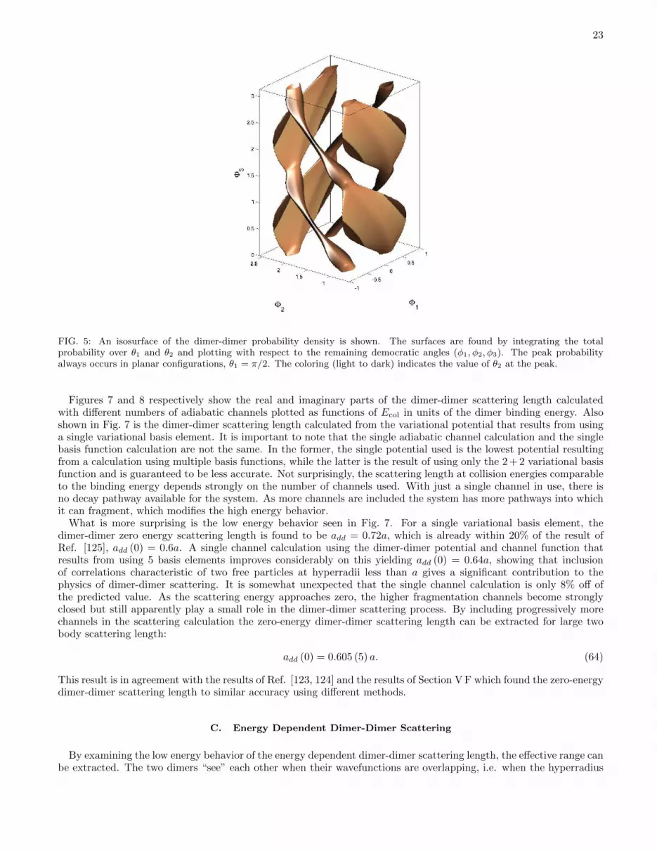
23

FIG. 5: An isosurface of the dimer-dimer probability density is shown. The surfaces are found by integrating the totalprobability over θ1 and θ2 and plotting with respect to the remaining democratic angles (φ1, φ2, φ3). The peak probabilityalways occurs in planar configurations, θ1 = π/2. The coloring (light to dark) indicates the value of θ2 at the peak.

Figures 7 and 8 respectively show the real and imaginary parts of the dimer-dimer scattering length calculatedwith different numbers of adiabatic channels plotted as functions of Ecol in units of the dimer binding energy. Alsoshown in Fig. 7 is the dimer-dimer scattering length calculated from the variational potential that results from usinga single variational basis element. It is important to note that the single adiabatic channel calculation and the singlebasis function calculation are not the same. In the former, the single potential used is the lowest potential resultingfrom a calculation using multiple basis functions, while the latter is the result of using only the 2 + 2 variational basisfunction and is guaranteed to be less accurate. Not surprisingly, the scattering length at collision energies comparableto the binding energy depends strongly on the number of channels used. With just a single channel in use, there isno decay pathway available for the system. As more channels are included the system has more pathways into whichit can fragment, which modifies the high energy behavior.

What is more surprising is the low energy behavior seen in Fig. 7. For a single variational basis element, thedimer-dimer zero energy scattering length is found to be add = 0.72a, which is already within 20% of the result ofRef. [125], add (0) = 0.6a. A single channel calculation using the dimer-dimer potential and channel function thatresults from using 5 basis elements improves considerably on this yielding add (0) = 0.64a, showing that inclusionof correlations characteristic of two free particles at hyperradii less than a gives a significant contribution to thephysics of dimer-dimer scattering. It is somewhat unexpected that the single channel calculation is only 8% off ofthe predicted value. As the scattering energy approaches zero, the higher fragmentation channels become stronglyclosed but still apparently play a small role in the dimer-dimer scattering process. By including progressively morechannels in the scattering calculation the zero-energy dimer-dimer scattering length can be extracted for large twobody scattering length:

add (0) = 0.605 (5) a. (64)

This result is in agreement with the results of Ref. [123, 124] and the results of Section V F which found the zero-energydimer-dimer scattering length to similar accuracy using different methods.

C. Energy Dependent Dimer-Dimer Scattering

By examining the low energy behavior of the energy dependent dimer-dimer scattering length, the effective range canbe extracted. The two dimers “see” each other when their wavefunctions are overlapping, i.e. when the hyperradius

24

FIG. 6: The same as Fig. 5, but using only the 2 + 2 function. The dashed gray lines are purely for perspective.

0.1 1 10 100 1000Ecol/Eb

-0.5

0

0.5

1

1.5

2

Re(a dd)/a

FIG. 7: The real part of the energy dependent dimer-dimer scattering length is shown in units of the atom-atom scatteringlength a, plotted versus the collision energy in units of the dimer binding energy. The calculation is carried out with one, two,three, four, and five adiabatic channels (blue, black, red, green, and purple curves respectively) from the adiabatic potentialcurves and couplings computed using 8 basis functions. The red dashed line shows add = 0.6a, the prediction of Ref. [127].

is approximately equal to the scattering length, R ∼ a. If one thinks of the effective range of an interaction asproportional to the size of the interaction region, then one would expect the effective range for dimer-dimer scatteringto be proportional to the scattering length. By fitting the low energy scattering phase shift to the effective rangeexpansion,

−1

add(E)= kdd cot δdd = − 1

add (0)+

1

2rddkdd

2 +O(kdd4) (65)

this intuitive behavior is born out, giving an effective range:

rdd = 0.13(1)a, (66)

25

0.1 1 10 100 1000Ecol/Eb

0

1

2

-Im(add)/a

FIG. 8: The imaginary part of the energy dependent dimer-dimer scattering length is shown in dimensions of a plotted versusthe collision energy in units of the binding energy. The calculation is carried out with one, two, three, four, and five adiabaticchannels (blue, black, red, green, and purple curves respectively) from the adiabatic potential curves and couplings computedusing 8 basis functions.

where a is the two-body scattering length. Figure 9 shows both the real and imaginary parts of the energy dependentdimer-dimer scattering length as a function of collision energy in units of the binding energy compared to the effectiverange expansion, Eq. (65). This clearly shows that, while the low energy behavior of dimer-dimer scattering iswell described by the effective range expansion, it is only accurate over a small range of collision energies. In fact,for collision energies larger than the binding energy, add (Ecol) actually turns over and decreases as dimer breakupchannels become open. Further, when the collision energy exceeds the dimer binding energy, Ecol = Eb, the dimer-dimer scattering length becomes complex, with an imaginary part that parameterizes inelastic processes. These resultsindicate that both the real and imaginary dimer-dimer scattering lengths are universal functions of the collision energy.Specifically, they are insensitive to the short range nature of the two-body interaction, for scattering lengths muchlarger than the two-body interaction length scale, r0. Because very few basis functions were used in these calculations,the results at higher energies, Eb Ecol ~2/mr2

0, are not well converged, though their qualitative nature is expectedto persist. Well above the dissociation threshold, the real part of add exhibits an oscillatory behavior. These oscillationsare caused by interference between different scattering pathways. As more basis functions are included and the highenergy results converge, the large number of available pathways generally washes out the oscillatory behavior andproduces incoherence , but the decrease in the real part of the add at higher energies is expected to survive as thecalculations become better converged.

The dependence of add on a at finite collision energy is particularly interesting. In the large a limit, the dimerbinding energy becomes Eb ≈ ~2/ma2, so that as a increases, the binding energy decreases. At the critical value ofthe scattering length,

ac =~√mEcol

,

the collision energy coincides with the binding energy, and the dimer-atom-atom channel becomes open. As a result(see Fig. 9), one expects the real part of add to turn over and remain finite for all values of a. This behavior isdemonstrated in Fig. 10 which compares the real part of the dimer-dimer scattering length at several fixed collisionenergies with the zero-energy result, add (0) = 0.6a. The scattering length scale has been fixed by setting the rangeof the interaction to be approximately the Van der Waals length of 40K, r0 ≈ 100 a.u. Another aspect of the finitecollision energy behavior is that at large scattering length, the dimer-atom-atom channels become open, and dimerdissociation is allowed. Thus, near unitarity the Fermi gas might be viewed as a coherent mixture of atoms and weaklybound dimers.

D. Dimer-dimer relaxation

A significant loss process in an ultracold gas of bosonic dimers is that of dimer-dimer relaxation, in which twodimers collide and in the process at least one of the dimers relaxes to a deeply bound two-body state. The extra

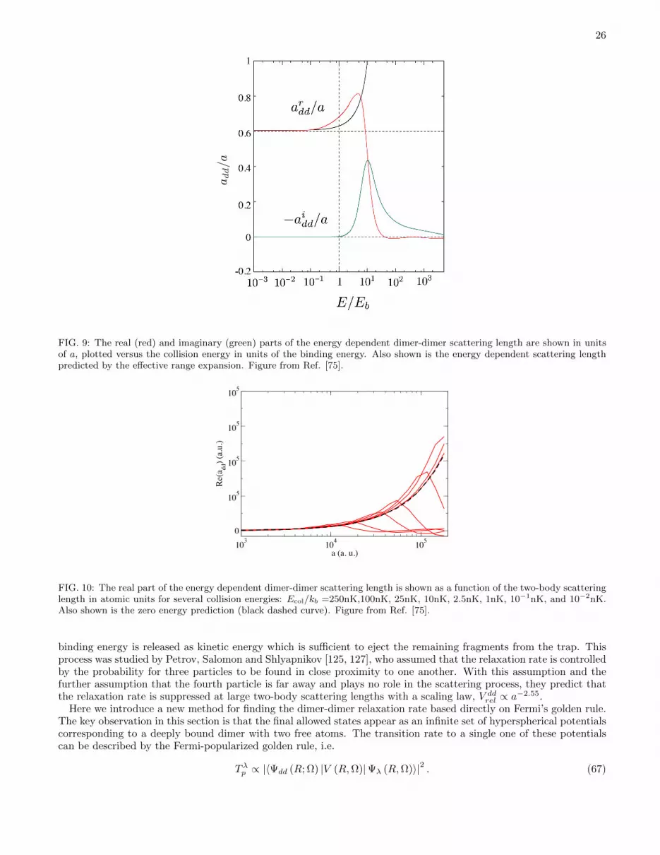
26

add/a

FIG. 9: The real (red) and imaginary (green) parts of the energy dependent dimer-dimer scattering length are shown in unitsof a, plotted versus the collision energy in units of the binding energy. Also shown is the energy dependent scattering lengthpredicted by the effective range expansion. Figure from Ref. [75].

103

104

105

a (a. u.)

0

105

105

105

105

Re(

a dd)

(a.u

.)

FIG. 10: The real part of the energy dependent dimer-dimer scattering length is shown as a function of the two-body scatteringlength in atomic units for several collision energies: Ecol/kb =250nK,100nK, 25nK, 10nK, 2.5nK, 1nK, 10−1nK, and 10−2nK.Also shown is the zero energy prediction (black dashed curve). Figure from Ref. [75].

binding energy is released as kinetic energy which is sufficient to eject the remaining fragments from the trap. Thisprocess was studied by Petrov, Salomon and Shlyapnikov [125, 127], who assumed that the relaxation rate is controlledby the probability for three particles to be found in close proximity to one another. With this assumption and thefurther assumption that the fourth particle is far away and plays no role in the scattering process, they predict thatthe relaxation rate is suppressed at large two-body scattering lengths with a scaling law, V ddrel ∝ a−2.55.

Here we introduce a new method for finding the dimer-dimer relaxation rate based directly on Fermi’s golden rule.The key observation in this section is that the final allowed states appear as an infinite set of hyperspherical potentialscorresponding to a deeply bound dimer with two free atoms. The transition rate to a single one of these potentialscan be described by the Fermi-popularized golden rule, i.e.

Tλp ∝ |〈Ψdd (R; Ω) |V (R,Ω)|Ψλ (R,Ω)〉|2 . (67)

27

Here Ψλ is the final outgoing state, Ψdd is the dimer-dimer wavefunction, and V (R,Ω) is the sum of the two-bodyinteractions. This matrix element and the sum of probabilities over final states are evaluated in Appendix E. Thefinal result of this analysis is expressed as an integral over the hyperradius,

V ddrel ∝∫PWKB (R)F (R)

Rκ (R)ρ (R) dR (68)

where PWKB (R) is the WKB probability density of the dimer-dimer wavefunction at hyperradius R, κ (R) is theWKB wavenumber:

κ (R) =

√2µ

~2

(Vdd (R) +

~2

2µ

1/4

R2− Ecol

). (69)

In Eq. (68) ρ (R) is the nearly constant density of final states, and F (R) is the probability for three particles to benear one another in the dimer-dimer wavefunction at hyperradius R:

F (R) = 〈Φdd (R; Ω) |f (R,Ω)|Φdd (R; Ω)〉 . (70)

Here Φdd is the hyperangular dimer-dimer channel function, and f (R,Ω) is a proximity function that is appreciableonly when three particles are all approximately within the range of the two-body interaction.

Equation (68) makes physical sense upon closer examination. It says that the rate at which a dimer relaxes to adeeper state is determined, with some extra factors, by the probability that three particles are close enough togetherso that two of them can fall into a deeply bound state and release the extra binding energy to the third particle.Figure 11 shows the integrand from Eq. (68) for several scattering lengths as a function of the hyperradius in unitsof the scattering length. This quantity can be interpreted as being proportional to the transition rate per unithyperradius, i.e. the probability that the transition will occur between R and R + dR. The full transition rate isdetermined by the nature of the interaction at short range and is not predictable using this method. By examining therelaxation rate as a function of scattering length, however, a scaling law can be extracted at each fixed hyperradius.

0.5 1 1.5 2R/a

Tp (

arbi

trar

y un

its)

FIG. 11: The integrand from Eq. (68) is shown for a = 50r0 (red),64r0 (green),80r0 (blue), and 100r0 (black) as a function ofR/a.

Figure 12 shows the relaxation rate per unit hyperradius for several fixed values of R/a as a function of the scatteringlength, a. The large a behavior in each case appears to follow a scaling law, but the scaling law changes with R/a.This behavior indicates that, contrary to the prediction of Ref. [127], when the integral in Eq. (68) is evaluated,the relaxation rate will not be determined by a simple power law. By integrating over different hyperradial regions,contributions to the transition rate from different processes can be extracted. For instance, if the integral in Eq. (68)is performed only over small hyperradii, R . 5r0, the result is the transition rate due to processes in which all four

28

particles are in close proximity. If the integral is evaluated over larger hyperradii, R > 10r0, the result is the rate dueto three-body processes influenced by the presence of the fourth particle.

FIG. 12: The logarithm of the integrand from Eq. (68) is shown for several fixed values of R as a function of a/r0

FIG. 13: The relaxation rate in a dimer-dimer collision is shown as a function of the atom-atom scattering length (see text).Figure from Ref. [75]

Figure 13 shows the relaxation rate as a function of the scattering length in atomic units as a solid line. In thisresult the range of the interaction is set to the van der Waals length of 40K, r0 ≈ 100 a.u. Also shown in Fig. 13are the contributions to this relaxation rate due to four-body processes (dashed blue curve), and due to three-bodyprocesses (dotted green curve). Also shown is the expected scaling law for transitions that occur at small hyperradius,R = 5r0. Because the hyperradius is small in this regime, the probability of three particles being in proximity is nearunity, meaning that the transition probability per unit hyperradius is determined by the probability that the systemcan tunnel through the repulsive potential seen in Fig. 3 at R . a. The universal repulsive potential in this regime[75, 101],

U (R) =~2

2µ

p20 − 1/4

R2, (71)

p0 = 2.55, (72)

leads to a scaling law for transitions in the small R regime that behaves as

V ddrel ∝ a1−2p0 = a−4.20. (73)

Figure 13 also shows the experimentally determined relaxation rates from Ref. [73]. Both the scaling law predicted in

29

Ref. [127] of a−2.55 and the prediction using Eq. (68) are consistent with the experimental data in the regime for 1000a.u.. a . 4000 a.u.. The experimental data for a > 3000 a.u. are in the regime where the average dimer separationis less than the dimer size, where the dimer-dimer scattering picture discussed here no longer applies.

E. Trapped four-body system

In this section we abandon the hyperspherical methods of the previous sections and examine the case of trappedfour-fermion systems. The four-body system in confined geometries has recently become computationally accessible.In particular, the trapped two-component Fermi system has been intensely studied in the last few-years and hasbecome a benchmark for different theories and universal predictions. One of the challenges present in the studyof universal four-body physics in dilute gases with short range forces is the description of disparate length scalesassociated with the large interpaticle distances and the short-range two-body interactions.

In this section, we analyze the spectrum, dynamics and universal properties of four-body solutions in confinedgeometries. The four-body system is described by a the model Hamiltonian

H =

2∑i=1

(−~2

2m1∇2i +

1

2m1ω

2r2i

)+

2∑i′=1

(−~2

2m2∇2i′ +

1

2m2ω

2r2i′

)+

2∑i=1

2∑i′=1

V (rii′) (74)

where unprimed indices label the fermionic species with mass m1, primed indices label the species with mass m2,and ri is the position vector of the ith fermion. The trapping frequency ω is assumed to be equal for both species.In order to facilitate a calculation with the CG method described in Section IV, we take the interaction potentialV to be a purely attractive Gaussian (see Eq. (40)) and tune the depth of V to give the desired (large) scatteringlength. The mass ratio κ is defined by m1/m2, and throughout the analysis we assume m1 ≥ m2. A trap length

a(i)ho =

√~/miω is defined for each species as well as a trap length associated with the pair aho =

√~/2µω, where

µ = m1m2/(m1 +m2). For equal mass systems, aho = a(1)ho = a

(2)ho .

This section reviews a series of predictions for the two-component four-fermion system. The spectrum and structuralproperties of the four-fermion system are analyzed throughout the BCS-BEC crossover, followed by an exploration ofthe system dynamics as the scattering length is tuned close to a Fano-Feshbach resonance. Finally, we review a seriesof numerical studies that confirm and quantify universal predictions.

1. Spectrum in the BCS-BEC crossover

To obtain the J = 0 spectra for the four-fermion system in the BCS-BEC crossover problem, the CG method(Section IV) is utilized to solve the time-independent Schrodinger equation for different values of a. Like mostnumerical methods, this method provides an adiabatic spectrum (in time), i.e., the energies of the spectrum arelabeled according to their energy values as a changes. The four-body spectra present a series of crossings or narrowavoided crossings when the scattering length is tuned across the BCS-BEC crossover. For this reason, it is convenientto use a representation where these narrow avoided crossings are treated diabatically, and the spectrum smoothlyevolves from the BCS to the BEC side. The diabatic representation is more relevant from the physical point of viewsince the diabatic states are usually associated with good or “approximately good” symmetries of the problem.

To illustrate the diabatization procedure, consider the spectrum of the four-fermion system in the strongly interact-ing region shown in Fig. 14. A series of crossings and avoided crossings occurs when the adiabatic parameter λ ≡ 1/ais varied in the strongly interacting region. The avoided crossings can be roughly characterized by their width ∆λ,the range where the two adiabatic energy curves are coupled. There are narrow crossings where ∆λ 1/aho andthere are wide crossings where ∆λ & 1/aho. To obtain smooth energy values, we use variation of the diabatizationprocedure presented in Ref. [128].

The objective of the diabatization algorithm is to make the one-to-one connection between states and energies inconsecutive points of the λ grid that maximize the sum of the overlaps between connected states. The diabatizationprocedure starts from the BCS (a < 0) side of the resonance and connects the states (and their energies) betweenconsecutive values of λ for which their overlap is maximum. When two initial energies connect to the same finalenergy, a refinement of the diabatization procedure is applied.

Diabatization is controlled by the spacing between consecutive values of λ given by ∆λg. If the width of the avoidedcrossing is smaller than ∆λg, then that crossing is diabatized. But if the width of the avoided crossing is larger than∆λg, then that crossing is not diabatized. Thus, ∆λg is selected so that narrow crossings are diabatized and wide

30

FIG. 14: Four-fermion energy spectrum as a function of λ = 1/a in the unitarity region with J = 0. The thin solid black linescorrespond to the adiabatic spectrum. The wide black line with circles is the diabatic ground state labeled ΨDD1. The bluecurve with circles is the diabatic first-excited state labeled ΨDD2, the wide red curve with circles is the diabatic state ΨDAA,and the wide green curve with circles is the diabatic state Ψ4A.

crossings remain adiabatic. For example, in Fig. 14 we see how this procedure diabatizes the narrow crossings of Ψ4A,however, wide crossings such as the one between ΨDAA and Ψ4A are still adiabatic in this representation.

This structure of avoided crossings permits a global view of the manner in which states evolve from weakly interactingfermions at a < 0 to all the different configurations of a Fermi gas at a > 0, i.e., molecular bosonic states, fermionicstates, and molecular Bose-Fermi mixtures. Furthermore, it allow us to visualize concretely the alternative pathwaysof the time-dependent sweep experiments.

The diabatic spectrum of the four-fermion system is presented in Fig. 15. The structure of avoided crossings iscomplicated because of two different thresholds exist, one corresponding to the dimer-atom-atom and one to thedimer-dimer state. We identify three different families of diabatic states in this spectrum. The dimer-dimer family,represented by the black and blue curves, describes the ground and excited dimer-dimer states. These states areseparated by approximately 2~ω on the BEC side. The dimer–two-atom family, represented by the red energy curves,follows the dimer binding energy. In the BEC limit, the dimer–two-atom family reproduces the degeneracies of threedistinguishable particles: a spin up atom, a spin down atom, and a dimer. The third family describes four-atombound states, for which the atoms form no dimers, and whose energy remains positive in the crossover region. In theBEC limit as a→ 0, the four-atom family reproduces the spectrum of the noninteracting four-body system.

The evolution of the N = 4 spectra through the BCS-BEC crossover region can be understood qualitatively byconsidering the important quantum numbers for the description of the dimer. For each vibrational excitation of 2~ωin the noninteracting limit, there is one state that diabatically becomes a dimer-dimer state. These states correspond

qualitatively to states where the relative angular momentum of two spin-up–spin-down pairs is zero [L↑↓rel = 0], and therelative angular momentum between the pairs is also zero. The spin-up–spin-down pairs are in the lowest vibrationalstate. In the weakly interacting BCS limit, where the degeneracy of the vibrational states is broken, pair-pair statescorrespond to the lowest states.

A direct and more concrete way to visualize the structure of the spectrum is to analyze the evolution of the adiabatichyperspherical potential curves. Figure 16 presents the four-fermion adiabatic hyperspherical potential curves Uν(R),obtained with the correlated Gaussian hyperspherical method (CGHS). Panel (a) presents the potential curves in theBCS regime, which are clearly grouped into families. Potential curves belonging to the same family are degeneratein the noninteracting limit. Thus, the weak interactions in the BCS regime break the degeneracies of the potentialcurves forming these families of potential curves. Panel (b) describes the system in the BEC regime. In this case,the description of the system is quite clear. The lowest potential curve is more than twice as deep as the rest of thecurves and is associated with the dimer-dimer threshold. The family of dimer-dimer states live mainly in the lowestpotential curve. The remainder of the displayed potential curves are associated with the dimer–two-atom threshold.The dimer–two-atom states are mainly described by this family of potential curves. A third family of potential curves,not shown in Fig. 16 (b), describes four-atom states. This family of potential curves has a different large-R asymptoticbehavior.

In order to benchmark the four-body energies, Figure 17 compares CG results with fixed-node diffusion Monte

Carlo (FN-DMC) results carried out by Blume.[130] From the ground-state energy, the energy crossover curve Λ(κ)4 ,

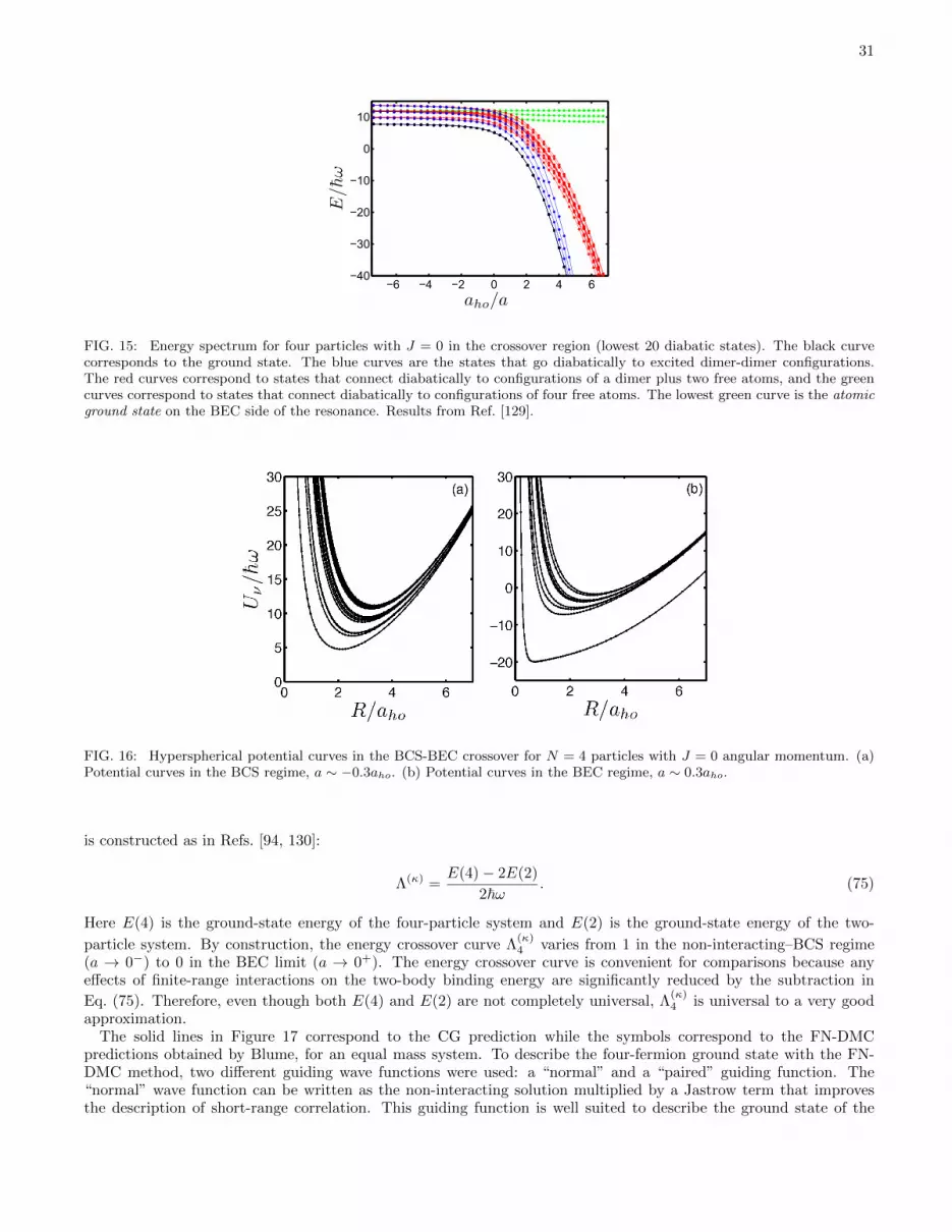
31

−6 −4 −2 0 2 4 6−40

−30

−20

−10

0

10

aho/as

E/hω

FIG. 15: Energy spectrum for four particles with J = 0 in the crossover region (lowest 20 diabatic states). The black curvecorresponds to the ground state. The blue curves are the states that go diabatically to excited dimer-dimer configurations.The red curves correspond to states that connect diabatically to configurations of a dimer plus two free atoms, and the greencurves correspond to states that connect diabatically to configurations of four free atoms. The lowest green curve is the atomicground state on the BEC side of the resonance. Results from Ref. [129].

FIG. 16: Hyperspherical potential curves in the BCS-BEC crossover for N = 4 particles with J = 0 angular momentum. (a)Potential curves in the BCS regime, a ∼ −0.3aho. (b) Potential curves in the BEC regime, a ∼ 0.3aho.

is constructed as in Refs. [94, 130]:

Λ(κ) =E(4)− 2E(2)

2~ω. (75)

Here E(4) is the ground-state energy of the four-particle system and E(2) is the ground-state energy of the two-

particle system. By construction, the energy crossover curve Λ(κ)4 varies from 1 in the non-interacting–BCS regime

(a → 0−) to 0 in the BEC limit (a → 0+). The energy crossover curve is convenient for comparisons because anyeffects of finite-range interactions on the two-body binding energy are significantly reduced by the subtraction in

Eq. (75). Therefore, even though both E(4) and E(2) are not completely universal, Λ(κ)4 is universal to a very good

approximation.The solid lines in Figure 17 correspond to the CG prediction while the symbols correspond to the FN-DMC

predictions obtained by Blume, for an equal mass system. To describe the four-fermion ground state with the FN-DMC method, two different guiding wave functions were used: a “normal” and a “paired” guiding function. The“normal” wave function can be written as the non-interacting solution multiplied by a Jastrow term that improvesthe description of short-range correlation. This guiding function is well suited to describe the ground state of the

32

system in the BCS-unitarity regime. The “paired” wave function is constructed as an antisymmetrized product oftwo-body solutions and leads to a good description of the ground state in the BEC-unitarity regime. In order toreduce finite range corrections, the ranges r0 of the two-body potentials used in Fig. 17 are set to be much smaller

than the oscillator lengths, i.e., r0 ≈ 0.01a(2µ)ho . By analyzing the dependence of the energy on the finite range r0,

we can extrapolate the zero-range prediction and estimate the deviation in the crossover curve Λ(κ)4 from the zero

range predictions. Such analysis estimates a 1% deviation in the crossover curve presented in Fig. 17. For example,

at unitarity the CG energies are E = 5.027~ω for r0 = 0.01a(2µ)ho and E = 5.099~ω for r0 = 0.05a

(2µ)ho . After a more

careful analysis of the range dependence we obtain an extrapolated zero-range value of E = 5.009~ω. For comparison,

the FN-DMC energy for the square well potential with r0 = 0.01a(2µ)ho is E = 5.069(9), which agrees well with the

energy calculated by the CG approach.

6 4 2 0 2 4 60.0

0.2

0.4

0.6

0.8

1.0

ahoa

1

FIG. 17: Energy crossover curve Λ(κ)4 as a function of a

(2µ)ho /a for κ = 1. Solid lines are calculated by the CG approach, and

symbols by the FN-DMC method. Adapted from Ref. [130].

A test of the validity of the guiding function in FN-DMC calculations is fundamental for an accurate description ofmany-body fermionic systems. Comparisons, such as the one presented in Fig. 17 represent much-needed benchmarktests for the “normal” and “paired” trial wave-functions used in the FN-DMC approach [130] The good agreement

between these two numerical methods suggests that, first, Λ(κ)4 is indeed universal; and second, that both numerical

methods accurately describe the BCS-BEC crossover for this four-body system.

F. Extraction of dimer-dimer collisional properties

In the BEC limit, the lowest four body levels describe different vibrational states of a dimer-dimer configuration.Therefore, the systems can be treated effectively in this limit as two-particle systems. A comparison between the twoparticle solutions and the N = 4 solutions allows us to extract information on the effective dimer-dimer interactions.

To model the effective dimer-dimer interaction we introduce a zero-range pseudopotential. Since the size of thedimers are of the order of a, the range of the effective potentials should also be of order of a. Accordingly, effectiverange effects are discussed using an energy-dependent scattering length. Inclusion of the scattering length energydependence is well-known to extend the validity of the zero-range pseudopotential when applied to the scattering oftwo atoms with finite-range potentials under external confinement [131, 132]. This energy dependence is includedhere through the effective range expansion

− 1

add(Ecol)≈ − 1

add+

1

2k2rdd. (76)

Here add(Ecol) is the energy-dependent dimer-dimer scattering length parameterized by the (zero-energy) scatteringlength add and the effective range rdd. The momentum k is associated with the relative kinetic energy of the dimer.Thus, k2/2µ = Ecol where Ecol = E4b − 2E2b. The appropriate reduced mass µ is µdd = M/2, where M is the massof the bosonic molecules, M = m1 +m2.

Using the effective range expansion [Eq. (65)], the regularized zero-range potential V (r) [133] takes the formV (r) = g(E)δ(r)(∂/∂r)r. The scattering strength g is parameterized by the scattering length add and the effective

33

range rdd, i.e.,

g(E) =2π~2 add

µ

[1− µEcolrddadd

~2

]−1

. (77)

The J = 0 spectrum of the two particle trapped system is given by [131, 132]

√2

Γ(−Ecol2~ω + 3

4

)Γ(−Ecol2~ω + 1

4

) =a

(µ)ho

add(Ecol). (78)

Equation (78) is a transcendental equation that can be easily solved numerically. The solutions of Eq. (78) are obtainedas functions of the add and rdd parameters and fitted to the numerical results. The calculation can be carried out atdifferent values of the two-body scattering length a and, in this way, one obtains a reliable estimation of add and rdd.

Since the properties of weakly-bound dimers are controlled by the scattering length, it is natural to assume that theproperties of dimer-dimer interactions are controlled only by a. This implies that add and rdd should be proportionalto the two-body scattering length a. Therefore, we propose expressions of the form add = cdda and rdd = ddda. Theparameters cdd and ddd are obtained by fitting the zero-range two-particle solution to the dimer-dimer states of theN = 4 system.

0 0.2 0.4 0.6 0.80

0.5

1

as/a(M )ho

2

2.5

3

(Ei(4)

−2E

(2))/hω

4

4.5

5(c)

(b)

(a)

a/a(M)ho

FIG. 18: Four-body energies of the three energetically lowest-lying dimer-dimer states as a function of a/a(M)ho for κ = 8.

Panel (a) shows the energetically lowest-lying energy level (i = 0), panel (b) shows the energetically second-lowest (i = 1) andpanel (c) shows the energetically third-lowest state (i = 2). Circles and crosses show our CG and FN-DMC results, respectively.Solid lines show the zero-range model results. Figure from Ref. [130].

The results in Fig. 18 illustrate the fitting procedure. The circles in Figs. 18(a)–(c) show the lowest-lying dimer-dimer energy levels, referred to as Ei(4), where i = 0–2 with the center-of-mass energy and the dimer-binding energysubtracted. These energies correspond to a two-heavy two-light four-body system with mass ratio κ = 8. Solidlines represent the energy-dependent zero-range pseudopotential predictions obtained by fitting the two-boson model[Eq. (78)] to the four-body energies. The range of atom-atom scattering lengths, a, over which the four-fermion systemcan be described by the two-boson model is significantly extended by the inclusion of the effective range rdd. Suchinclusion also allows for a more stable and reliable determination of add.

The crosses in Fig. 18(a) correspond to FN-DMC energies for the energetically lowest-lying dimer-dimer state.The Blume FN-DMC energies, presented in Ref. [130], are found to be slightly higher than the CG energies, thedeviation increasing with a. This increasing deviation might be attributed to the variational implications of thefixed-node constraint. The functional form of the nodal surface used in the FN-DMC calculations was constructed fornoninteracting dimers and should be best in the very deep BEC regime. Application of the two-boson model and thefitting procedure to the Blume FN-DMC energies provides an alternative determination of add and rdd. The increasingdeviation between the FN-DMC and CG energies with increasing a explains why the effective range predicted by theanalysis of the FN-DMC energies is somewhat larger than that predicted by the analysis of the CG approach (seediscussion of Fig. 19 below).

The formation of few-body states, such as trimers or tetramers, can affect the scattering properties and limit the

34

TABLE II: The dimer-dimer scattering length, add, and dimer-dimer effective range, rdd, obtained using (a) the CG spectrumand (b) the FN-DMC energies. The reported uncertainties reflect the uncertainties due to the fitting procedure; e.g., thepotential limitations of the FN-DMC method to accurately describe the energetically lowest-lying gas-like stateare not includedhere (see Sec. IIIB of Ref. [130]).

κ add/a (a) add/a (b) rdd/a (a) rdd/a (b)

1 0.608(2) 0.64(1) 0.13(2) 0.12(4)

4 0.77(1) 0.79(1) 0.15(1) 0.23(1)

8 0.96(1) 0.98(1) 0.28(1) 0.38(2)

12 1.10(1) 1.08(2) 0.39(2) 0.55(2)

16 1.20(1) 1.21(3) 0.55(2) 0.60(5)

20 1.27(2) 1.26(5) 0.68(2) 0.74(5)

applicability of the two-boson model. For example, the lowest four-body energy for κ = 1, constitutes the true groundstate of the system, i.e., no energetically lower-lying bound trimer or tetramer states with JΠ = 0+ symmetry exist.However, for larger mass ratios, bound trimer and tetramer states exist. These few-body states can in principle beassociated with either universal Efimov or nonuniversal physics. Even in the regime where few-body bound states exist,the four-body spectrum contains universal states that are separated by approximately 2~ω and are best describedas two weakly-interacting composite bosons. For fixed a (a > 0), the energy of these “dimer-dimer states” changessmoothly as a function of κ even in the regime where bound trimer states appear. Thus, our two-boson model andthe fitting procedure can be extended to this regime of mass ratios.

Table II and Fig. 19 summarizes the dimer-dimer scattering length and effective range for for selected values ofthe mass ratio κ. Circles and crosses in Fig. 19 correspond to the dimer-dimer scattering length, add, extracted fromthe energies calculated by the CG and the FN-DMC approach, respectively, as a function of κ. The add two-bosonmodel predictions compare well with those calculated by Petrov et al. within a zero-range framework [134] (solidline in Fig. 19). The existence of Efimov states limited Petrov et al. calculations to κ . 13.6 since beyond thismass ratio a three-body parameter is needed to solve the zero-range four-body equations. As mentioned above, thefour-body solutions for a finite range potential include deeply-bound solutions which correspond to either a trimer-atom or a tetramer. The trimer-atom states affect the dimer-dimer scattering properties only when the dimer-dimerconfiguration is close in energy to the trimer-atom energy, which usually corresponds to a narrow window in two-bodyscattering length. Away from this window, the dimer-dimer states are well described by the two-boson mode whichpredicts a smooth increase of the add up to mass ratio κ = 20.

Note that the existence of energetically-open atom-trimer channels at the dimer-dimer collisional energy providesa decay mechanism for the dimers. Clearly, such a decay mechanism cannot be captured within this rather simpletwo-boson model and a more sophisticated treatment should be used to extract the inelastic scattering properties. A

0 5 10 15 200

0.5

1

κ

r dd/as,

add/as

FIG. 19: Circles and crosses show add/a as a function of κ extracted from the four-fermion CG and FN-DMC energies,respectively. For comparison, a solid line shows the results from Fig. 3 of Ref. [134]. Diamonds and squares show rdd/aextracted from the four-fermion CG and FN-DMC energies, respectively. Figure from Ref. [130].

recent theoretical study found good agreement with the two-boson model predictions beyond 13.6 [135].The two-boson model also provides estimates for the dimer-dimer effective range, rdd (shown as diamonds and

squares in Fig. 19). The uncertainty of rdd obtained from the CG approach is estimated to be about 10%; this

35

uncertainty is expected to be larger for the results extracted from the FN-DMC energies since those calculations onlyinclude one energy curve. As shown in Fig. 19, the ratio rdd/a increases from about 0.2 for κ = 1 to about 0.5 forκ = 20. The existence of a finite effective range can be attributed to the effective broad soft-core potential thatthe dimers experience [134]. Ref. [130] predicts rdd as a function of the mass ratio κ. The large value obtained forrdd suggests that effective-range corrections may need to be considered in order to accurately describe the physics ofmolecular Fermi gases.

To conclude, we have shown that studies of few-body trapped systems can be used to extract information aboutthe collisional properties of free systems. Dimer-dimer scattering lengths can be extracted by analyzing the trappedfew-body spectrum for different two-body scattering length values. Furthermore, energy-dependent corrections to addcan also be obtained with this method.

G. Structural properties

The analysis of the BCS-BEC crossover spectrum can be complemented by an analysis of the wave functions andtheir structural properties. The present section determines the one-body densities and pair-distribution functions fortwo-component Fermi systems in the crossover regime. The averaged radial densities, ρi(r), are normalized such that4π∫ρi(r)r

2dr = 1; 4πr2ρi(r) represents the probability of finding a particle with mass mi at a distance r from thecenter of the trap. Here we focus in the m1 = m2 case, where we find that the radial one-body densities ρ1(r) andρ2(r) coincide and we can omit the species label. The unequal mass case, in which the radial one-body densitiesρ1(r) and ρ2(r) differ, will not be considered here but was discussed in Ref. [124]. Also, the averaged radial pairdistribution functions, Pij(r), are normalized so that 4π

∫Pij(r)r

2dr = 1; 4πr2Pij(r) represents the probability offinding a particle of mass mi and a particle of mass mj at a distance r from each other.

These structural properties are computed using the CG method. Since we are only focusing J = 0 states, all thestructural properties presented here are spherically symmetric. The structural properties are calculated using thefollowing general expression:

4πr2F (r) = 〈Ψn|δ(x− r)|Ψn〉 =

∫dr1...drNδ(x− r)|Ψn(r1, r1′ , ..., rN1 , rN2)|2. (79)

Here, F (r) is a generic structural property, e.g. the density profiles ρ1 or ρ2, the interspecies pair-correlation functionP12, or the intraspecies pair-correlation functions P11 or P22. x is the length of the coordinate vector that describes thestructural property. For ρ1 and ρ2, x = r1 and x = r1′ , respectively. For P12, x is the interparticle distance betweenopposite-spin or different species, x = r11′ . For P11 and P22, x is the same-spin or same-species interparticle distance,with x = r12 and x = r1′2′ , respectively. To evaluate 4πr2F (r), Ψn is expanded in the CG basis set, permitting theintegral in Eq. (79) to be carried out analytically.

0.0 0.5 1.0 1.5 2.00.0

0.1

0.2

0.3

0.4

0.5

raho

Ρraho3

FIG. 20: Single particle density profiles for interaction strength across the crossover. Thick curves correspond to numericalresults: a = −aho (solid curves), a = ±∞ (dashed curves) and a = 0.1aho (dash-dotted curves). Thin curves correspond toanalytic limiting solutions: noninteracting four-fermion prediction (less peaked), dimer-dimer solution in the BEC limit (morepeaked).

Figure 20 presents the single particle density profiles for different interaction strength across the crossover. The

36

radial density profiles of the equal mass four-fermion system smoothly evolve from the noninteracting solution (lesspeaked thin black curve) in the BCS limit to the prediction of dimer-dimer model in the BEC limit (more peaked thinblack line). In the BEC limit (a→ 0+), the density profile coincides with that of two point like bosonic dimers, i.e.,

ρ(r) = exp(−r2/a(M)ho )/(a

(M)ho

√π)3. For small but finite positive scattering lengths (dash-dotted curve), the density

profiles is broader which can be attributed to both the finite size of the dimers and the effective repulsive dimer-dimerinteraction.

Next, we analyze the opposite-spin pair distribution function. For a zero-range pseudopotential, the opposite-spinpair-correlation function obeys a boundary condition [136, 137]

[rP12(r)]′r=0

[rP12(r)]r=0= −2

a. (80)

This behavior is a direct consequence of the Bethe-Peierls (B-P) boundary condition[r12Ψ(r12)]′r12=0/[r12Ψ(r12)]r12=0 = −1/a. The factor of 2 in Eq. (80) appears because the pair correlation

function is proportional to the square of the wave function, i.e., P12(r) ∝ Ψ(r12)2. A direct consequence of Eq. (80)is that at unitarity, i.e., when |a| =∞, r2P12(r) has zero slope at r → 0.

0 1 2 3 40

0.2

0.4

0.6

0.8

1

r/aho

4πr2P12(r)/a−1

ho

FIG. 21: Pair-distribution functions P12(r), multiplied by r2, for equal-mass–two-component Fermi systems with N = 2(dashed curve) and N = 4 (solid curve). The N = 2 pair-correlation function has an arbitrary norm selected to match theN = 4 pair correlation in the small r regime.

The numerical verification of Eq. (80) is challenging. For systems with finite range interactions, Eq. (80) is valid ina narrow regime of r values. For a < 0, Eq. (80) is valid when r is much larger than the range of the potential andmuch smaller than the mean interparticle distance, i.e., the r0 r aho regime. For a > 0, Eq. (80) is valid when ris much larger than the range of the potential and much smaller than the size of the dimer (given by a) and the meaninterparticle distance, i.e., the r0 r min[a, aho] regime. This regime is almost nonexistent for our numericalcalculations, because we consider only the aho/r0 = 100 case.

The pair distribution function changes considerably as interactions are tuned across the BCS-BEC crossover. Fig-ure 22 shows the pair distribution function P12(r) along the crossover for equal mass systems [κ = 1] in the BCS(solid lines), unitary (dashed lines) and BEC (dash-dotted lines) regime. As attractive interactions increase, the pairdistribution function evolves from a single peak structure to a double peak structure. The single peak structureis usually associated to solutions where spin-up-spin-down interparticle distances are mainly controlled by a singlelength scale and all particles are roughly at the same distance. This single peak structure appears in the BCS regimesince the attraction is not strong enough to bind the particles and the typical interparticle distance is set mainlyby the external trapping potential. The multi peak structures in pair distribution functions are generally associatedto solutions were more than one length scale control the interspecies interparticle distance. In this case, a doublepeak structure already appears at unitarity and becomes more pronounce in the BEC regime. The peak at small rindicates the formation of weakly bound dimers and its width is associated to the size of the dimers. The broaderpeak between 1 aho and 2 aho is related to the presence of larger atom-atom length scales set approximately by thetypical dimer-dimer separation in the harmonic oscillator potential. Understanding the BEC solutions as two dimersin a trap implies that the four-body configurations includes two interspecies distances of the size of the dimer (short)and two interspecies distances of the size of the trap (large). Thus, the probability of finding two particles fromdifferent species at short distances should be equal to the probability of finding them at large distances. This premisecan is verified by comparing the area under first and second peaks in the P12(r)r2 plot. Finally, note that in moving

37

through the BCS-BEC crossover region, the slope of r2P12(r) at small r changes from positive to zero to negative, asis predicted by Eq. (80).

0 1 2 3 40.0

0.2

0.4

0.6

0.8

1.0

raho

4Πr2P12ra ho1

FIG. 22: Pair-distribution functions P12(r), multiplied by r2, for equal-mass–two-component Fermi systems with N = 4 andJ = 0. The solid curve corresponds to a = −aho (BCS regime), dashed curve 1/a = 0 (unitarity), and dashed-dotted a = aho(BEC regime). Adapted from Ref. [94].

0 0.05 0.1 0.15 0.20

2

4

6

8

4πr2P12(r)/a−1

ho

r/aho

0 0.5 1 1.5 2 2.5 30

0.2

0.4 (a)

(b)

FIG. 23: (a) Circles show the pair-distribution function, P12(r), multiplied by r2, for a = 0.1aho (BEC regime). For comparison,the blue dash-dotted line shows P12(r)r2 for two atoms of mass m with the same scattering length but normalized to 1/2, thered dashed line shows P12(r)r2 for two trapped bosonic molecules of mass 2m interacting through a repulsive effective potentialwith add = 0.6a, and the green dotted line shows P12(r)r2 for two trapped noninteracting bosonic molecules of mass 2m. Panel(b) shows a blow-up of the small r region. Figure from Ref. [94].

The dimer-dimer model can be quantitatively tested in the deep BEC regime (0 < a aho). In this regime, the twopeaks of the pair distribution function are well separated and can be independently analyzed. The small-r correspondsto dimer formation and is well described by the pair-distribution function multiplied by r2 and normalized to 1/2, fortwo trapped atoms with a = 0.1aho (dash-dotted curve). The large-r peak describes dimer-dimer correlations and iswell described by the pair distribution function of two bosonic molecules of mass 2m in a harmonic trap (dotted line).The agreement is quite good but it can be improved by including the effective dimer-dimer interaction corrections.The dashed curve, almost indistinguishable from the large r part of the pair-distribution function for the four-particlesystem, shows dimer-dimer model prediction including the effective repulsive potential with dimer-dimer scatteringlength add ≈ 0.6a [130, 134]. Thus, even though the dimer-dimer interaction corrections are small, they are noticeablyin the pair distribution function.

1. Dynamics across the BCS-BEC crossover region

The diabatic representation can be used to ramp an initial configuration through the BCS-BEC crossover region,mimicking experiments carried out at different laboratories at JILA and Rice University. The initial configuration is

38

propagated using the time-dependent Schrodinger equation,

i~d |Ψ〉dt

= H[λ(t)] |Ψ〉 . (81)

The time dependence of the Hamiltonian comes entirely from that of λ(t) ≡ 1/a(t) term. In this case, we focuson unidirectional ramps. Starting from the ground state on the BCS side, the parameter λ is ramped through theresonance to the BEC side at different speeds, ν = dλ

dt . The relevant dimensionless speed quantity is ξ = ahoν/ω. Theparameter ξ can be rewritten in terms of ν, the density of the system ρ and the particle mass to relate few-body andmany-body predictions [138]. This reformulated version of ξ (see Ref. [129]) agrees with the functional form of theLandau-Zener parameter obtained in Refs. [139, 140]. The dependence of the Landau-Zener parameter on ρ has beenexperimentally verified [141].

To propagate the initial configuration, we use the diabatic representation obtained previously in Sec V E 1. First,we divide the BCS-BEC crossover range into sectors. Starting from the BCS side at λ ≈ λBCS and finishing atthe BEC side at λ ≈ λBEC , the BCS-BEC crossover is divided into 40–80 sectors. At the middle of each sector,the time-independent Hamiltonian is diagonalized using the CG method. For four-body systems, thousands of CGbasis functions are usually needed to describe the spectrum. While in principle this basis set could be used to solveEq. (81), in practice this large basis would make the numerical propagation very slow. Instead, we use the diabaticrepresentation obtained at the middle of the j-th sector to expand the time-dependent wave function throughout thatsector, i.e.,

|Ψ(t)〉 =

Nd∑i

cji (t) |Ψji 〉 . (82)

Here, |Ψji 〉 is the diabatic basis function i of sector j, and Nd is the number of diabatic states considered. The time

dependence only appears in the complex coefficients cji (t). Upon selecting only the lowest 20–100 diabatic states atthat point, we drastically reduce the size of the Hamiltonian matrix in Eq. (81). Since the inverse scattering length λchanges very little in each sector, the relevant diabatic states are well described by this reduced basis set throughoutthe sector. The time-dependent Schrodinger equation, Eq. (81), is propagated from one edge of the sector to the otherusing an adaptive-step Runge-Kutta method.

To understand the time propagation of this system, consider the way the probabilities evolve as the system transitsthe BCS-BEC crossover region. At each point of the time propagation, the probability to reside in state i is given bypi(t) = |cji (t)|2. Here j denotes the sector that includes λ(t). The probabilities of evolving into a given family canbe found by summing the probabilities of all states belonging to the same family. For two particles, there are twofamilies, the dimer family, which only includes the lowest state, and the two-atom family, which includes the rest of

the states. In this case, the appropriate definitions are pd(t) = |cj1(t)|2, and P2a(t) =∑Ndi=2 |c

ji (t)|2.

The N = 4 system has four relevant families: the ground state, the excited dimer-dimer states, the dimer–two-atomstates, and the four-atom states. These families are characterized by the probabilities pg(t), pdd(t), pd2a(t), and p4a(t),respectively.

Figure 24 presents examples of the numerical time evolution of an N = 4 system during a unidirectional rampat constant speed from the BCS to the BEC side. As expected, the probability of staying in the ground statedecreases with increasing ramp speed. The probability of evolving into the final four-atom configuration increaseswith speed, which is in agreement with the projection argument. The transfer of probability occurs mainly in thestrongly interacting regime, −2 . aho/a . 2. In this region, the diabatic states are sometimes mixed, producingjumps in the probabilities. For example, around aho/a ≈ 1, the red and blue curves have a kink due to an avoidedcrossing between an excited dimer-dimer state and a dimer–two-atom state.

The probabilities at the end of the time evolution can also be studied as functions of the speed ξ. Before analyz-ing these numerical results, however, consider first the simple Landau-Zener model that provides insights into ournumerical calculations.

In its simplest form, the Landau-Zener model, considers a two-level system whose energy difference depends linearlyon the adiabatic parameter λ, i.e., ε1 − ε2 = αλ, and are coupled by ε12 independent of λ. The time evolution ofthis model can be easily solved, yielding the nonadiabatic transition probability Tna to evolve into a final adiabaticstate different from the initial adiabatic state after the parameter λ is varied through an avoided crossing. To obtainthis probability, the time-dependent Schrodinger equation is propagated starting at t = −∞ [with ψ(t) = ψ1] tot = +∞. The nonadiabatic probability is then given by Tna = | 〈ψ(+∞)|ψ2〉 |2. Landau and Zener solved thisproblem analytically and showed that

Tna(ν) = e−δ, (83)

39

0

0.5

1

0

0.5

1

P−6 −4 −2 0 2 4 6

0

0.5

1

aho/as

(a)

(b)

(c)

FIG. 24: Probabilities of different families of the N = 4 system during a unidirectional ramp at constant speed dλ/dt from theBCS to the BEC side. The initial configuration is |ΨBCS

1 〉. The black curve corresponds to pg(t). The blue curve corresponds topdd(t). The red curve corresponds to pd2a(t), and the green curve corresponds to p4a(t). (a) Probabilities obtained for rampingat a speed of ξ ≈ 13. (b) ξ ≈ 52. (c) ξ ≈ 128

.

where δ = 2πε212/(αν).Our goal is to use this simple expression to describe each of the important nonadiabatic transitions in the four-

fermion description. However, equation (83) is not very useful in its current form when it comes to analyzingnumerical results since it requires a knowledge of nonadiabatic quantities such as α and ε12. ε12 can be estimatedfrom the difference between adiabatic energy curves at the closest approach. But, in the four-body problem, α is verydifficult to extract because there is a rich structure of avoided crossings. Nevertheless, Clark [142] showed how α canbe obtained from an analysis of the P-matrix coupling between two adiabatic states. In the Landau-Zener model, theP-matrix between the two adiabatic states |ψ+〉 and |ψ−〉 is

P+−(λ) = 〈ψ+|dψ−dλ〉 =

α

4ε12

1

1 + [αλ/(2ε12)]2, (84)

and has a characteristic Lorentzian form whose parameter is directly related to α and ε12.Analysis of the spectrum and the P-matrices permits an identification of the states Ψi and Ψj involved in the most

important nonadiabatic transitions, and a determination of the Landau-Zener transition probability

Tij(ν) = e−δij = e−ηijξ . (85)

The Landau-Zener parameter δij characterizes the transition and is extracted by analyzing the spectrum, while theP-matrix is obtained from the numerical description of the adiabatic states using the Hellmann-Feynman theorem.

Figure 25 (b) displays the results obtained from the numerical time propagation. The black symbols correspond tothe dimer-dimer ground state. The blue symbols correspond to the excited dimer-dimer family, the red symbols to thedimer–two-atom family, and the green symbols to the four-atom family. For slow ramps (small ξ), the probability offorming a “condensate”, i.e., remaining in the ground state, is large. For intermediate ramps, the greatest probabilityis to break one bond and end up with a dimer plus two particles. For fast ramps (large ξ), the probability of stayingin the atomic ground state on the BEC side is dominant. The probability of the system evolving into an exciteddimer-dimer configuration remains small for all ramping speeds.

To analyze these transitions within the Landau-Zener approximation, the partially diabatic states have been labeledaccording to their energies in the BCS regime. This labeling is arbitrary since many of the states are almost degenerate.Based on the P-matrix couplings, the possible pathways point towards the states that are most likely important.Starting from the ground state, note that |Ψ1〉 has important couplings with states |Ψ2〉 and |Ψ5〉. Here, |Ψ2〉 isthe first excited dimer-dimer state, i.e., the lowest state of the excited dimer-dimer family. State |Ψ5〉 is the firstexcited state of the dimer–two-atom configuration. Since an important probability is transferred to states |Ψ2〉 and|Ψ5〉, we analyze the couplings of these states to follow the flow of probability. State |Ψ2〉 has an important couplingwith |Ψ5〉, and state |Ψ2〉 has an important coupling with |Ψ13〉. Here, |Ψ13〉 is the lowest state of the four-atom

40

configuration, i.e., the atomic ground state on the BEC side. Figure 25 (a) presents the energy curves of these fourstates. Conveniently, each of these states represents a different configuration. For that reason, this is the minimalset of states that can describe the numerical results. While more states could be included in the analysis, here onlythe simplest possible case is considered. The P-matrix analysis also reveals the order in which the transition usually

0 50 1000

0.2

0.4

0.6

0.8

1

ξ

P

−5 0 5−5

0

5

10

15

aho/a0

E/hω

(a) (b)

FIG. 25: (a) Energy of the most important states amenable to a Landau-Zener description, through the BCS-BEC crossoverregime.The black curve corresponds to |Ψ1〉 which represents the ground state configuration. The blue curve corresponds to|Ψ2〉 which represents the excited dimer-dimer configuration. The red curve corresponds to |Ψ5〉 which represents a dimerplus two atoms. The green curve corresponds to |Ψ13〉 which represents the lowest four-atom configuration. (b) Probabilityof ending up in a given configuration after the ramp, as a function of the dimensionless speed parameter ξ. The symbolscorrespond to the numerical evolution, while the curves correspond to the Landau-Zener approximation. The colors follow thesame convention as Figure (a). Results from Ref. [129].

occurs. The order of the peaks reveals the following sequence: the first transition is 1→ 2, then 2→ 5, then 1→ 5,and finally 5→ 13. The Landau-Zener prediction for this sequence is

p1 = (1− T1,2)(1− T1,5),

p2 = T1,2(1− T2,5),

p5 = ((1− T1,2)T1,5 + T2,5T1,2)(1− T5,13), (86)

p13 = ((1− T1,2)T1,5 + T2,5T1,2)T5,13.

Again, the sum of all these probabilities is, by construction, unity. The Landau-Zener parameters obtained from theP-matrix analysis are η12 ≈ 5.4, η15 ≈ 6.6, η25 ≈ 2.1 and η5,13 ≈ 13.8. The sequence of Landau-Zener transitionsin the model shows good agreement with the numerical results even though many possible transitions have beenneglected in the approximate model.

2. Universal properties

The universal properties of two-component Fermi gases interacting through s-wave collisions has been intensivelystudied in recent years. Some particularly important research has been carried out concerning the universal propertiesof four-fermion systems. Here we select two studies that benchmark the universal behavior of four-fermion systems.

The specific point in the strongly-interacting region where the s-wave interaction strength reaches its maximalvalue, is usually called unitarity. Unitarity is alternatively characterized by a divergent s-wave scattering length,|a| =∞. If inelastic two-body scattering channels are energetically open, the scattering length is complex and it doesnot diverge all the way to infinity, but the following discussion assumes that such inelastic processes can be neglected.In this situation, if the range of the interaction is much smaller than the typical interparticle distance and if thescattering length is divergent, then no relevant length scale exists that can characterize the interaction. This situationis similar to the noninteracting limit, where the absence of interactions implies, of course, the absence of a lengthscale that describes the interaction. The absence of a length scale that describes the interaction allows us to extractthe functional form of various quantities via dimensional analysis. Furthermore, it allows us to relate quantities atunitarity to those in the noninteracting limit.

Dimensional analysis becomes particularly simple in the hyperspherical framework for a noninteracting or unitary

41

system in free space, where the hyperradius is the only coordinate with dimensions of length. Since the potential curveshave units of energy and the only length scale is given by R, it follows that U(R) ∝ 1/R2. This is equivalent to sayingthat the potential curves at unitarity are proportional to the noninteracting potential curves, i.e.,U(R) ∝ UNI(R), sincethe noninteracting potential curves have the form 1/R2. The resulting predictions have been derived in Refs. [143, 144].

100

101

102

0

20

40

60

80

100

120

R/r0

2μR

2Uν(R

)/h2

FIG. 26: Hyperspherical potential curves at unitarity for the 4-fermion system multiplied by 2µR2/~2. The solid lines representthe predictions extracted from the spectrum obtained with the CG method. The symbols correspond to direct evaluation ofthe potential curves with the CGHS method. Solid lines correspond to predictions of the large R behavior of the potentialcurves extracted from the analysis of the excitation spectrum of the four-fermion trapped system.

The four-fermion potential curves calculated at unitarity using CGHS methods allow us to test the premise ofuniversality at the four-body level. Figure 26 presents predictions for the lowest 20 adiabatic potential curves fora Gaussian interaction model potential. At large R the potential curves become proportional to 1/R2 as predictedby the universal theory. This behavior of the potential curves can be used to understand universal predictions fortrapped systems such as the virial theorem and the energy spacing of the trapped spectrum.

The notion of universality extends beyond the unitarity regime and can be applied to any finite scattering length.Recently, Tan was able to derive a series of relations between different observables in two-component Fermi sys-tems [145–147]. These relations were obtained under the premise of universality and are a consequence of the wave-function behavior when two particles come close together (which is well described by the Bethe-Peierls boundarycondition). The universal Tan relations connect the energy, the expectation value of the trapping potential, the pairand momentum distribution functions of two-component Fermi systems through a quantity termed the integratedcontact intensity I(a).

10 5 0 5 10

1

10

100

ahoa

Ia ho

FIG. 27: Integrated contact intensity obtained in four different ways: through the analysis of the energy dependence on a (solidcurve), virial theorem (dashed curve), momentum distribution (blue symbols), and pair correlation function (red symbols).The solid and dashed curves are essentially indistinguishable on this scale. Figure adapted from Ref. [148].

Blume and Daily investigated the Tan relations for a trapped four-fermion system[148]. Using the CG method,they extracted the spectrum, the pair correlation function, the momentum distribution and the external potentialexpectation value for determining I(a) in four different ways. Figure 27 presents a comparison of the different predic-

42

tions for the contact intensity. The excellent agreement between the different predictions numerically demonstratesthe validity of the Tan relations. Furthermore, it quantifies the contact intensity for the four-fermion system, whichcan serve as a benchmark for further studies.

VI. SUMMARY

This review has concentrated on recent developments in the four-body problem, emphasizing those insights thathave either used hyperspherical coordinate techniques directly, or else which have benefited indirectly from thoseinsights. The utility of formulating the few-body or even the many-body problem in hyperspherical coordinates wasglimpsed early on by some of the pioneers in the field such as Delves[31, 32], Smirnov and Shitikova[149], Macek[38],Lin[40], Fano[150], Kuppermann[98], and Aquilanti[55]. This class of methods has been especially valuable for studyingultracold collisions in recent years, and ultracold applications have been the focus of this overview.

Bosonic four-body systems could not be discussed in much detail in this article, owing to length constraints, butthey have provided an important proving ground for many of the methods discussed in the present review. Earlyideas on 3-body recombination for three bosons or for three nonidentical fermions that arose first from an adiabatichyperspherical perspective[10, 11] have since been confirmed and developed further, with many useful new insightsfrom independent theoretical perspectives. The few-body system receiving the most attention over the years hasbeen the three-body problem, both with and without long range Coulombic interactions. The exciting headwayrepresented by that body of literature has had some extensions to handle nontrivial reactive processes for systemswith four interacting particles,[151] and in a handful of studies, for systems with many more particles.[152–158]

Numerous questions still remain to be addressed in this field, aiming in the long run towards not only answeringquestions of universality in the ultracold, but also towards developing systematic ways of handling four-body chemicalreaction dynamics at the fully quantum level. A large parameter space also remains to be explored just in the ultracoldlimit of the four-body problem, such as varying mass ratios for fermionic and for bosonic systems as well as mixedBose-Fermi systems.

VII. ACKNOWLEDGMENTS

Many of the results described in this review were developed in close collaboration with Doerte Blume, and wedeeply appreciate her contributions and insights. We also thank Brett Esry for numerous informative discussions andfor access to some of his results prior to publication. This project was supported by NSF.

Appendix A: Hyperangular coordinates

As with Jacobi coordinates, there is no unique way to construct the hyperangles of a system. In this section weconstruct the hyperangular coordinates used in the four-fermion problem. The choice of hyperangular parameterizationhas physical meaning. Different parameterizations can be used to describe different correlations within the system.Also, in the case of body-fixed coordinates, hyperspherical coordinates can be used to remove the Euler angles of solidrotation, reducing the dimensionality of the system.

1. Delves coordinates

Unfortunately, or possibly fortuitously depending on your view point, there is no unique way to define the hy-perangles in a given system. Here we use a simple, standardized method of defining them used by many others[38, 97, 152, 157–159] in the form of the so called Delves coordinates [31, 32]. We will begin by examining a wellknown example of hyperspherical coordinates, that of normal spherical polar coordinates. Clearly these coordinatescan be used to describe the relative motion of 2 particles in 3 dimensions or the position of a single particle in atrap-centered coordinate system, but it can also be used in less obvious ways. For instance, spherical polar anglesmay be used to describe the relative motion of 4 particles in 1 dimension.

43

FIG. 28: The tree that gives the standard spherical coordinates for a 3 dimensional system is shown.

FIG. 29: The canonical tree that gives a hyperangular parameterization for a d dimensional system is shown.

The components of a three dimensional vector, r, can be written in terms of a radius and two angles as

x = r cosφ sin θ, (A1)

y = r sinφ sin θ, (A2)

z = r cos θ. (A3)

This parameterization can be represented in a simple tree structure shown in Fig. 28. The end points of the treerepresent each component of the vector r, and each node in the tree is represents an angle. Also associated with eachnode is a sub radius. For the lowest node the “subradius” is merely the total length of the vector, r. For the upper

node the subradius is merely the cylindrical radius ρ =√x2 + y2. Using the tree structure from Fig. 28, a set of rules

can be developed for extracting the parameterization of Eqs. (A1), (A2), and (A3). Starting at the bottom node withtotal radius, r, move up through the tree to the desired coordinate. For each move through the tree, if you move tothe left (right) from a node multiply by the sine (cosine) of the angle associated with that node. Continue until youreach the Cartesian component.

This procedure can be generalized readily from three to d dimensions. Start by building a tree with d free ends andd − 1 nodes, associate an angle with each node and follow the above rules. Using the tree structure, starting at thebottom node with total hyperradius, R, move up through the tree to the desired coordinate. If you move to the left(right) from a node, multiply by the sine (cosine) of the angle associated with that node. Continue until you havereach the desired Cartesian component. A specific tree for d dimensions is shown in Fig. 29. Following the rules thistree gives the hyperangular representation

xn = R cosαn−1

d−1∏j=n

sinαj , (A4)

0 ≤ αj ≤ π, j = 2, ..., d− 1

0 ≤ α1 ≤ 2π

44

FIG. 30: The tree structure used to correlate two subspaces to a single hyperradius.

where cosα0 ≡ 1 andd−1∏j=d

sinαj ≡ 1. This can also be written as

tanαn =

√∑nj=1 x

2j

xn+1, (A5)

n = 1, 2, 3, ..., d− 1.

This hyperspherical tree has been dubbed the canonical tree [91, 97] as it is simple to construct and very easy to addmore dimensions to.

To avoid double counting, the range that the hyperangles take on is restricted depending on how many free branchesare attached to the node corresponding to a given angle. If the node has two free branches, then the angle takes onthe full range 0 to 2π. If the node has one free branch attached, the angle goes from 0 to π. If the node has no freebranches attached to it, the associated angle goes from 0 to π/2. Following these rules for the canonical tree givesthe ranges of the angles αi,

0 ≤ α1 ≤ 2π,

0 ≤ αi ≤ π, i = 2, ..., d− 1.

Another slightly more abstract way of considering this construction is to start by breaking the d dimensional spaceinto two subspaces of dimension d1 and d2, and assuming that these two subspaces are already described by two setsof sub-hyperspherical coordinates, (R1,Ω1) and (R2,Ω2). With these assumptions all that remains is to correlate thesub-hyperradii. This is done by following the type of procedure described above using the tree structure shown inFig. 30,

R1 = R sinα, (A6)

R2 = R cosα,

where α is now the final hyperangle in the system. Using this procedure recursively, one can define the hyperangles inthe subspaces until the only remaining subspaces are the individual Cartesian components of the total d dimensionalspace. The concept of dividing the total space up into subspaces will prove very or the purpose of constructing basisfunctions.

As a final example of hyperangular parameterizations, we introduce a parameterization for N 3-dimensional vectors

ρiNi=1. One could break each vector up into its individual components and use the canonical parameterization fromEq. (A4), but this removes much of the spatial physical intuition that one could bring to bear, such as the individualspatial angular momentum corresponding to each vector. Instead one can use a variation on the canonical tree shownin Fig. 31. On first glance, this tree might seem the same as the canonical tree shown in Fig. 29. In this case, though,the large dot at the end of each branch represents the spherical polar sub-tree of the form shown in Fig. 28 for eachvector ρi. Using this tree structure and following the rules outlined above, 2N of the 3N − 1 hyperangles are givenby the normal spherical polar angles for each vector, (θ1, φ1, θ2, φ2, ..., θN , φN ). The remaining N − 1 hyperangles are

45

FIG. 31: The tree structure used to parameterize the hyperangles for N three dimensional vectors is shown. Note that the dotat the end of each branch in the tree on the left stands for a spherical polar tree.

given by

tanαi =

√∑ij=1 ρ

2j

ρi+1, (A7)

0 ≤ αi ≤π

2,

i = 1, 2, 3, ..., N − 1.

where ρi is the length of the ith vector. It will be shown in the next section that this parameterization is useful whenspatial angular momentum plays a role in the problem of interest. For completeness, following the rules laid out inAppendix A, the hyperangular volume element that results from this parameterization is given by

dΩ =

(N∏i=1

dωi

)N−1∏j=1

cos2 αj sin3j−1 αj

where ωi is the normal spherical polar differential volume for ρi.

The first hyperangular parameterization used here is in the form of Eq. (A7) for three 3D vectors. The hyperradiusis defined in the same way as in Eq. (B1),

R2 =

d∑i=1

x2i , (A8)

where each xi is a Cartesian component of one of the Jacobi vectors. The hyperspherical trees that will be used forthe four fermion problem will of the type in Fig. 31 in which N vectors are described by the spherical polar angles ofeach vector and a set of hyperangles correlating the lengths of each vector. Specifically, the hyperangles are definedby the tree shown in Fig. 32 combined with the spherical polar angles of each Jacobi vector. Following the rules

FIG. 32: The hyperspherical tree used to parameterize the hyperangular coordinates in the four-fermion problem is shown. SeeChapter 2 or Ref. [97] for details.

46

described above gives the hyperangles,

ασl,m = tan−1 |ρσl ||ρσm|

, (A9)

ασlm,n = tan−1

√|ρσl |

2+ |ρσm|2

|ρσn|.

Here the superscript σ = s, i1, i2 indicates which Jacobi system is being used, while l,m, n indicate the three Jacobivectors from that system. In principle there are six of these hyperangular coordinate systems that can be constructedfrom each set of Jacobi vectors giving a total of 18 different hyperangular systems. Fortunately we will not need all ofthese to tackle the four fermion problem. If one considers two particles, say 1 and 2, the tree defined by Fig. 32 withσ = i1, l = 2,m = 3 and n = 1 can be decomposed into two subtrees. The right branch describes the hyperangularbehavior of the dimer alone, while the left branch describes the behavior of the remaining three body system composedof a dimer and two free particles. This type of decomposition will be important for evaluating kinetic energy matrixelements and defining basis functions.

Using the recursive definition of the hyperangular momentum operator in Eq. (B4) the total hyperangular momen-tum operator can be written in terms of the hyperangular coordinates as

Λ2 =∆1

(ασlm,n

)− 1

sin2 ασlm,n sinασl,m cosασl,m

[∂

∂ασl,m

]2

sinασl,m cosασl,m (A10)

+l2l

sin2 ασlm,n sin2 ασm,n+

l2msin2 ασlm,n cos2 ασm,n

+l2n

cos2 ασlm,n,

∆1

(ασlm,n

)=

−1

sin2 ασlm,n cosασlm,n

1

sinασlm,n

∂

∂ασlm,nsinασlm,n

∂

∂ασlm,nsin2 ασlm,n cosασlm,n,

where ll, lm and ln are the normal spatial angular momentum operators for each Jacobi vector. This can also bewritten directly from Eq. (B4) as

Λ2 = ∆1

(ασlm,n

)+

Λ2l,m

sin2 αlm,n+

l2ncos2 ασlm,n

, (A11)

Λ2l,m = − 1

sinασl,m cosασl,m

[∂

∂ασl,m

]2

sinασl,m cosασl,m +l2l

sin2 ασm,n+

l2mcos2 ασm,n

,

where all of the hyperangular behavior above the second node in Fig. 32 is described by a sub-hyperangular momen-tum, Λ2

lm,n.Constructing the hyperspherical harmonics for the four-body system is accomplished following the procedure in

Section B giving

Y(4b)[λλl,mll,lm,ln] (Ω) =N33

lllmλl,mN63λl,mln,λ

sinλl,m (αlm,n) cosln (αlm,n)Pλl,m+5/2,ln+1

(λ−λl,m−ln)/2 (cos 2αlm,n) (A12)

×Nλl,mll,lm

sinll (αl,m) coslm (αl,m)P ll+1,lm+1(λl,m−ll−lm)/2 (cos 2αl,m)

× yllml (ωl) ylmmm (ωm) ylnmn (ωn) ,

where Pα,βγ (x) is a Jacobi polynomial of order γ, ylm (ω) is a normal spherical harmonic with spherical polar solid

angle ω, and Ndeabc is a normalization constant [91, 97]:

Ndeabc =

[(2c+ d+ e− 2) Γ

(a+b+c+d+e−2

2

) (c−a−b

2

)!

Γ(c+a−b+d

2

)Γ(c+b−a+e

2

) ]1/2

.

In Eq. (A12) the degeneracy quantum number µ has been replaced with an explicit tabulation of the hyperangularmomentum quantum numbers, i.e. λµ → [λλl,mll, lm, ln]. The total four-body hyperspherical harmonics satisfy the

eigenvalue equation Λ2Y(4b)[λλl,mll,lm,ln] (Ω) = λ (λ+ 7)Y

(4b)[λλl,mll,lm,ln] (Ω). The sub-harmonics that are eigenfunctions of

47

Λ2l,m can be found as well:

Y(3b)[λl,mll,lm] (Ωl,m) =N33

ll,lmλl,msinll (αl,m) coslm (αl,m)P ll+1,lm+1

(λl,m−ll−lm)/2 (cos 2αl,m) (A13)

× yllml (ωl) ylmmm (ωm) .

Here the superscript, (3b), indicates that this eigenfunction behaves as a 3-body hyperspherical harmonic. Forinstance if a hyperspherical tree is used with Jacobi vectors defined in the i1 interaction coordinate system and l = 1,m = 3, and n = 2, this three-body harmonic describes the free-space behavior of a dimer with two free particles. The

three body harmonics obey the eigenvalue equation, Λ2l,mY

(3b)[λl,mll,lm] (Ωl,m) = λl,m (λl,m + 4)Y

(3b)[λl,mll,lm] (Ωl,m). The

restrictions on the values of λ and λl,m are

λl,m = ll + lm + 2j, (A14)

λ = λl,m + ln + 2k

= ll + lm + ln + 2j + 2k,

where j, k = 0, 1, 2, .... The quantum numbers ll, lm and ln are the spatial angular momentum quantum numbersassociated with Jacobi vectors ρl, ρm and ρn respectively, and each has a z-projection quantum number associatedwith it which we have suppressed in Eqs. (A12) and (A13).

2. Democratic coordinates

Using Delves coordinates greatly simplifies evaluating hyperangular momentum matrix elements, but it still leavesthe 8 dimensional space of hyperangles. I will only be considering systems with total angular momentum L = 0.Therefore it is convenient to move into a body-fixed coordinate system, as the final wavefunction for the four-bodyproblem will not depend on the Euler angles that produce a solid rotation of the system. Removing the Eulerangle dependence is accomplished by transforming into the so-called democratic, or body-fixed coordinates. Four-body democratic coordinates are developed in several references (see Refs. [55, 98, 99]). In this work we use theparameterization of Aquilanti and Cavalli. For a detailed derivation of the coordinate system see their work in Ref.[55].

At the heart of democratic coordinates is a rotation from a space fixed frame to a body fixed frame:

% = DT (α, β, γ)%bf (A15)

where % is the matrix of Jacobi vectors defined in Eq. (C12), %bf is the set of body fixed Jacobi coordinates, andD (α, β, γ) is an Euler rotation matrix defined in the standard way as

D =

cosα − sinα 0

sinα cosα 0

0 0 1

cosβ 0 sinβ

0 1 0

− sinβ 0 cosβ

cos γ − sin γ 0

sin γ cos γ 0

0 0 1

. (A16)

The “˜” in Eq. (A15) indicates a transpose has been taken.The body-fixed coordinates are defined in a system whose axes are defined by the principle moments of inertia,

I1, I2 and I3. In this coordinate system the body-fixed Jacobi coordinates are given by

%bf = ΠD (φ1, φ2, φ3) , (A17)

where D is defined in the same way as in Eq. (A16) with φ1, φ2 and φ3 replacing α, β, and γ. Π is a 3× 3 diagonalmatrix whose diagonals are given by ξ1, ξ2 and ξ3 which are parameterized by the hyperradius and two hyperangles

48

Θ1 and Θ2:

ξ1 =R√3

cos Θ1,

ξ2 =R√3

√3 sin2 Θ1 sin2 Θ2 + cos2 Θ1, (A18)

ξ3 =R√3

√3 sin2 Θ1 cos2 Θ2 + cos2 Θ1.

To avoid double counting and to allow for different chiralities, Θ1 and Θ2 are restricted to 0 ≤ Θ1 ≤ π and 0 ≤ Θ2 ≤π/4. With this parameterization the moments of inertia are given by

I1µ

= ξ22 + ξ2

3 =R2

3

(2 + sin2 Θ1

),

I2µ

= ξ21 + ξ2

3 =R2

3

(3 sin2 Θ1 cos2 Θ2 + 2 cos2 Θ1

), (A19)

I3µ

= ξ21 + ξ2

2 =R2

3

(3 sin2 Θ1 sin2 Θ2 + 2 cos2 Θ1

).

The hyperradius in terms of the principle moments of inertia can be then written as R2 = ξ21 + ξ2

2 + ξ23 =

(I1 + I2 + I3) /2µ.With this parameterization, all 8 hyperangles have been defined. The first three are the Euler angles α, β, γ,

which are external degrees of freedom describing solid rotations of the four body system. The two angles, Θ1 andΘ2, defined in Eq. (A18), describe the overall x, y and z extent of the four-body system in the body fixed frame.From Eq. (A19), if Θ1 = 0, π, then the principle moments of inertia are all equal, i.e. I1 = I2 = I3, meaning thatthe four particles are arranged at the vertices of a regular tetrahedron. When Θ1 = π/2, Eq. (A18) shows that theparticles are in a planar configuration. The remaining angles, φ1, φ2, φ3, are kinematic rotations within the system,and coalescence points and operations like particle exchange are described in these angles. Broadly speaking, thedemocratic angles Θ1 and Θ2 can be thought of as correlating the overall x, y, and z spatial extent of the four-bodysystem in the body-fixed frame, while the kinematic angles φ1, φ2, and φ3 parameterize the internal configuration ofthe particles.

Since transformations from one Jacobi set to another are merely rotation matrices (sometimes combined with aninversion), the democratic parameterization can always be written in the same form for any given Jacobi coordinatesystem. For example, the symmetry coordinates [Eq. (C3)] can be transformed into the second set interactioncoordinates [Eq. (C11)] using the kinematic rotation defined by Eq. (C15). If the democratic parameterizationdefined in Eqs. (A15) and (A17) is used, this transformation reads

%i2 = D (α, β, γ) ΠDT (φ1, φ2, φ3)Us→i2,

= D (α, β, γ) ΠDT (φ′1, φ′2, φ′3)

where we have used the fact that the product of two rotations in 3D is itself a rotation. From this it is clear thatwithin a given type of Jacobi coordinate (H-type or K-type), all coalescence points are equally well described. This isan important feature as it does not appear in Delves type coordinates, which are strongly dependent on which Jacobitree is used to define them. For the purposes of this paper, to make symmetrization of the wave function easier, wewill always define the body fixed coordinates in terms of the symmetry Jacobi system %s.

49

Putting this all together, the body-fixed Jacobi vectors in terms of the internal hyperangles can be defined:

ρs1x =R√3

cos Θ1 (cosφ1 cosφ2 cosφ3 − sinφ1 sinφ3) ,

ρs1y =R√3

√sin2 Θ1 sin2 Θ2 + cos2 Θ1 (sinφ1 cosφ2 cosφ3 + cosφ1 sinφ3) ,

ρs1z =−R√

3

√sin2 Θ1 cos2 Θ2 + cos2 Θ1 sinφ2 cosφ3, (A20)

ρs2x =−R√

3cos Θ1 (cosφ1 cosφ2 sinφ3 + sinφ1 cosφ3) ,

ρs2y =−R√

3

√sin2 Θ1 sin2 Θ2 + cos2 Θ1 (sinφ1 cosφ2 sinφ3 − cosφ1 cosφ3) ,

ρs2z =R√3

√sin2 Θ1 cos2 Θ2 + cos2 Θ1 sinφ2 sinφ3,

ρs3x =R√3

cos Θ1 cosφ1 sinφ2,

ρs3y =R√3

√sin2 Θ1 sin2 Θ2 + cos2 Θ1 sinφ1 sinφ2,

ρs3z =R√3

√sin2 Θ1 cos2 Θ2 + cos2 Θ1 cosφ2,

0 ≤ Θ1 ≤ π; 0 ≤ Θ2 ≤π

4,

0 ≤ φ1, φ2, φ3 ≤ π.

The restriction on the range of the internal hyperangles is to avoid double counting configurations and allows forconfigurations of different chirality .

By moving into democratic coordinates, the dimensionality of the four-body problem can be decreased from 9 to6, but, as with many simplifications, there is a cost. This cost comes in the form of the differential volume elementdΩ [55]:

dΩ = (dα sinβdβdγ)

√3 cos3 Θ2 sin3 Θ2 cos 2Θ2 sin9 Θ1[(

cos2 Θ2 + 3 sin2 Θ1 cos2 Θ2

) (cos2 Θ2 + 3 sin2 Θ1 sin2 Θ2

)]1/2 (A21)

× dΘ1dΘ2dφ1 sinφ2dφ2dφ3.

The first factor is purely from the Euler angle rotation and will always yield a factor of 8π2 for functions that areindependent of α, β and γ.

Another price that is paid using democratic coordinates comes in the form of the hyperangular momentum operator,

50

Λ2. In terms of the democratic hyperangles, Λ2 is quite complex and can be found in Ref. [55]:

Λ2 =−∆ (Θ1,Θ2) + 2µR2

I1

2 (I2 − I3)2

(L2

1 + J21

)+

I2

2 (I1 − I3)2

(L2

2 + J22

)+

I3

2 (I1 − I2)2

(L2

3 + J23

)

+2[I21 − (I2 − I3)

2]1/2

(I2 − I3)2 L1J1

+2[I22 − (I1 − I3)

2]1/2

(I1 − I3)2 L2J2

+2[I23 − (I1 − I2)

2]1/2

(I1 − I2)2 L3J3

,

where J is the total angular momentum operator, and

∆ (Θ1,Θ2) =1

sin7 Θ1

∂

∂Θ1sin7 Θ1

∂

∂Θ1+

2

sin2 Θ1

[∂2

∂Θ22

+ cot Θ1

(4

sin2 2Θ2

− 1

)∂

∂Θ1

]+

4

sin2 Θ1

1

4 sin 4Θ2

∂

∂Θ2sin 4Θ2

∂

∂Θ2+

2

3cot2 Θ1

[1 + 3 cos2 2Θ2

sin2 2Θ2

×(

1

4

∂2

∂Θ22

+cot 2Θ2

2

∂

∂Θ2

)− 1

sin 4θ2

∂

∂Θ2

]+ cot Θ1 cot 2Θ2

∂

∂Θ2

∂

∂Θ2

.

Terms in J2i are centrifugal contributions, terms in LiJi are Coriolis contributions and terms in L2

i are contributionsfrom internal kinematic angular momentum with

L = i~

sinφ1 cotφ2 cosφ1 − sinφ1

cosφ2

cosφ1 cotφ2 − sinφ1 −sinφ1

sinφ2

1 0 0

∂

∂φ1∂

∂φ2∂

∂φ3

.

Fortunately, the methods for evaluating matrix elements in what follows will not directly require this form of thehyperangular momentum, but it is included here for completeness.

The final element needed from the democratic coordinates is the inter-particle spacing. The ability to define thesewill be necessary to describe pairwise interactions and correlations. Using Eqs. (C1), (C13) and (A17),

|r12|2 =

√µ

µ12

[(%sbfUs→i1

)† (%sbfUs→i1

)]11, (A22)

|r13|2 =

√µ

µ13

[%s†bf%

sbf

]11, (A23)

|r14|2 =

√µ

µ14

[(%sbfUs→i2

)† (%sbfUs→i2

)]11, (A24)

|r23|2 =

√µ

µ23

[(%sbfUs→i2

)† (%sbfUs→i2

)]22, (A25)

|r24|2 =

√µ

µ24

[%s†bf%

sbf

]22, (A26)

|r34|2 =

√µ

µ23

[(%sbfUs→i1

)† (%sbfUs→i1

)]22, (A27)

51

where [ ]ij indicates the ijth element of a matrix. In this equation, only the body fixed Jacobi coordinates from Eq.

(A17) are used. This is because the unitary Euler rotation used to rotate into the body fixed frame is the same forall Jacobi coordinates canceling out the α, β, γ dependence in the inter-particle spacings.

Figure 2 shows the surfaces in φ1, φ2, φ3 for constant rij in a planar configuration for Θ2 = π/4, π/6, and π/12for equal mass particles. The φ1 coordinate axis has been transformed to φ1− πΘ (φ1 − π/2), where Θ (x) is the unitstep function, to emphasize the symmetry of the surfaces. The red surfaces correspond to the interacting particlesin the four-fermion system (r12, r14, r23 and r34) while the blue surfaces correspond to the identical fermions (r13

and r24). The identical particle surfaces surround a coalescence point that must be a Pauli exclusion node in thefinal four-body wave function. The simple nature of these coalescence points makes clear the reason for choosing tobase the democratic coordinates on the symmetry Jacobi vectors. The red surfaces will play an important role inthe pairwise interaction as these surfaces outline the valleys of the potential. As the system becomes more linear(Θ2 becomes smaller) it can be seen that the surfaces become broader in the φ1 direction. In fact, when Θ2 = 0 (inperfectly linear configurations) these surfaces become independent of φ1.

Appendix B: Hyperspherical harmonics

Strictly speaking an overview of hyperspherical coordinates is not really needed for this thesis, as there are manyexcellent existing works on the subject (see for instance [31, 32, 91, 97, 152, 159]). This section is included here forcompleteness in order to provide a more complete foundation for the variational basis functions used in this review.

To begin, consider a d dimensional Cartesian space whose coordinate axes are given by xidi=1. For the majorityof this review these coordinates are considered to be the components of a set of Jacobi vectors or the componentsof a set of trap centered vectors, but for now we proceed with a more abstract approach. The basic concept of thehyperradius is introduced here as

R2 =

d∑i=1

x2i . (B1)

While this definition is used here, often a mass scaling will be inserted. For instance in a trap centered system ofequal mass atoms an extra factor of 1/N , where N is the number of atoms, will be used to simplify the interpretationof the hyperradius. For the purposes of this section, though, this definition will be adequate. With Eq. (B1), the ddimensional Laplacian can be rewritten in terms of the hyperradius [91, 97]:

∇2 =

d∑i=1

∂2

∂x2i

=1

Rd−1

∂

∂RRd−1 ∂

∂R− Λ2

R2. (B2)

In this equation Λ is called the hyperangular momentum, or grand angular momentum operator, the square of whichis given by

Λ2 =∑i>j

− |Λij |2 , (B3)

Λij = xi∂

∂xj− xj

∂

∂xi.

Already the d dimensional Laplacian has a rather pleasing form reminiscent of its 3D counterpart. In fact if d is takento 3, Eq. (51) reduces exactly to the three dimensional Laplacian in spherical coordinates, and Λ becomes merely thenormal spatial angular momentum operator. To proceed from here a way of defining the remaining d− 1 degrees offreedom in terms of angles is needed.

The hyperangular momentum operator in terms of hyperangular coordinates can be found by using the fact thateach subset of Cartesian components is itself a Cartesian vector space. With that in mind, consider the hypersphericaltree given by Fig. 30. By writing the Laplacian for each subspace in terms of the sub-hyperradii R1 and R2 and thesub-hyperangular momentum operators Λ1 and Λ2 the total hyperangular momentum operator can be extracted [91].

52

It is

Λ2 =−1

sin(d1−1)/2 α cos(d2−1)/2 α

∂2

∂α2sin(d1−1)/2 α cos(d2−1)/2 α (B4)

+Λ2

1 + (d1 − 1) (d1 − 3) /4

sin2 α+

Λ22 + (d2 − 1) (d2 − 3) /4

cos2 α− (d− 1) (d− 3) + 1

4.

where α is defined as in Eq. (A6) and Λi is the sub-hyperangular momentum of the subspace of dimension di. If oneof the subspaces corresponds to a single Cartesian component then the sub-hyperangular momentum for that spaceis zero, i.e. if di = 1 then Λ2

i = 0. To find Λ21 (Λ2

2), ones needs only to apply Eq. (B4) recursively to each subspace.In this way, there is a sub-hyperangular momentum operator associated with each node in any given hypersphericaltree.

It is useful to be able to diagonalize the hyperangular momentum operator. The eigenfunctions of Λ2 are detailedin several references (See Refs. [38, 97, 159] for example), and the method of constructing them is given in AppendixA. These functions, Yλµ (Ω), are called hyperspherical harmonics. Their eigenvalue equation is

Λ2Yλµ (Ω) = λ (λ+ d− 2)Yλµ (Ω) , (B5)

where λ = 0, 1, 2, ... is the hyperangular momentum quantum number. The index µ enumerates the degeneracy foreach λ and can be thought of as the collection of sub-hyperangular momentum quantum numbers that result from agiven tree. Hyperspherical harmonics are also constructed as to diagonalize the sub-hyperangular momenta of eachnode in a given hyperspherical tree, e.g.

Λ21Yλµ (Ω) = λ1 (λ1 + d1 − 2)Yλµ (Ω) , (B6)

where λ1 = 0, 1, 2, ... is the sub-hyperangular momentum quantum number associated with Λ21. The total hyperangular

momentum quantum number λ is limited by the relation

λ = |λ1|+ |λ2|+ 2n, (B7)

where n is a non-negative integer. The absolute values in this case are there to allow for when either d1 or d2 are 2. Inthis special case the hyperangular momentum quantum number λi associated with the two dimensional subspace canbe negative, as with the magnetic quantum number, m, in spherical polar coordinates. Equation (B7) only applies ifboth d1 and d2 are greater than 1. If, for instance d2 = 1, then the restriction takes on the form

λ = |λ1|+ n.

The behavior illustrated in Eq. (B6) clearly demonstrates why the parameterization shown in Fig. 31 is useful.Each three dimensional spherical polar subtree will have a spatial angular momentum and z-projection associatedwith it, e.g.

l2i Yλµ (Ω) = li (li + 1)Yλµ (Ω) ,

where l2i is the square of the angular momentum operator for the ith vector. This property allows for addition of angularmomentum in the normal way, through sums over magnetic quantum numbers and Clebsch-Gordan coefficients. Nowthat the hyperspherical harmonics are defined, it is useful to examine a simple example applying them.

Appendix C: Jacobi Coordinate systems and Kinematic rotations

Here we detail the variety of coordinate systems that are used to describe the four-fermion problem in the adiabatichyperspherical framework and the necessary transformations to describe one set in terms of another. The coordinatesystems used here are not only needed to describe correlations between particles, they also allow the system to bereduced in dimensionality by removing the center of mass motion and moving into a body fixed frame. H-type Jacobicoordinates are constructed by considering the separation vector for two two-body subsystems, and the separationvector between the centers of mass of those two subsystems. K-type Jacobi coordinates are constructed in an iterativeway by first constructing a three body coordinate set, and then taking the separation vector between the fourthparticle and the center of mass of the three particle sub-system.

53

1. Jacobi coordinates: H-trees vs K-trees: fragmentation and symmetry considerations

The first and most obvious symmetry in the four-body Hamiltonian is that of translational symmetry. By describingthe system in the center of mass frame, the dimensionality of the system can be reduced from d = 12 to d = 9. Thisis done with the use of Jacobi coordinates. In the interest of brevity, We consider here only those coordinates directlyrelevant to the four-fermion problem. These coordinates may be broken into two sets, H-type and K-type, shownschematically in Fig. 1.

H-type Jacobi coordinates are constructed by considering the separation vector for two two-body subsystems, andthe separation vector between the centers of mass of those two subsystems, i.e.

ρHσ1 =

√µijµ

(ri − rj) ,

ρHσ2 =

√µklµ

(rk − rl) , (C1)

ρHσ3 =

√µij,klµ

(miri +mjrjmi +mj

− mkrk +mlrlmk +ml

),

ρcm =(m1r1 +m2r2 +m3r3 +m4r4)

m1 +m2 +m3 +m4,

µij =mimj

mi +mj, µij,kl =

(mi +mj) (ml +mk)

m1 +m2 +m3 +m4.

Here the superscript σ enumerates the 24 different H-type coordinates that may be obtained through particle per-mutation, ρcm is the position of center of mass of the four-body system, and µ is an arbitrary reduced mass for thefour-body system. The prefactors in each Jacobi vector, which are given in terms of the various reduced masses inthe problem, are chosen to give the so-called mass scaled Jacobi vectors. The kinetic energy in these coordinates canbe written as

−4∑i=1

~2

2mi∇2ri = − ~2

2M∇2ρcm −

~2

2µ

3∑j=1

∇2ρj ,

where M is the total mass of the four particles. The reduced mass, µ, can be chosen to preserve the differentialvolume element for the full 3D problem, ensuring that d3ρσ1d

3ρσ2d3ρσ3d

3ρcm = d3r1d3r2d

3r3d3r4:

µ =

(m1m2m3m4

m1 +m2 +m3 +m4

)1/3

.

Physically, the H-type coordinates are useful for describing correlations between two particles, for example a two bodybound state or a symmetry between two particles, or two separate two-body correlations.

When two particles coalesce [e.g. when ri = rj in Eq. (C1)], the H-type coordinate system reduces to a three bodysystem with two of the four particles acting like a single particle with the combined mass of its constituents:

ρHσ1 = 0,

ρHσ2 =

√µklµ

(rk − rl) ,

ρHσ3 =

√µij,klµ

(ri −

mkrk +mlrlmk +ml

).

Locating these “coalescence points” on the surface of the hypersphere is crucial for accurately describing the inter-actions between particles, and the coordinate reduction described above will prove useful for the construction of avariational basis set.

K-type Jacobi coordinates are constructed in an iterative way by first constructing a three body coordinate set, andthen taking the separation vector between the fourth particle and the center of mass of the three particle sub-system,

54

yielding

ρKσ1 =

√µijµ

(ri − rj) ,

ρKσ2 =

√µij,kµ

(miri +mjrjmi +mj

−mkrk

), (C2)

ρKσ3 =

√µijk,lµ

(miri +mjrj +mkrk

mi +mj +mk−mlrl

),

ρcm =(m1r1 +m2r2 +m3r3 +m4r4)

m1 +m2 +m3 +m4,

µij =mimj

mi +mj, µij,k =

(mi +mj)mk

mi +mj +mk,

µijk,l =(mi +mj +mk)ml

m1 +m2 +m3 +m4.

Again σ enumerates the 24 different K-type coordinates that result from particle permutations. Examining Fig. 1shows that K-type Jacobi coordinate systems are useful for describing correlations between three particles within thefour particle system. In the four fermion system, there are no weakly bound trimer states meaning that K-type Jacobicoordinates will not be used here, but the methods described in this report can be easily generalized to include thesetype of states. Unless explicitly stated all Jacobi coordinates from here on will be of the H-type, and for notationalsimplicity, we will drop the H superscripts.

a. Coalescence points and permutation symmetry

The proper description of coalescence points is crucial for describing two-body interactions, but they are alsoimportant for describing points of symmetry. For instance if two identical fermions are on top of one another it isknown that the wave function must vanish at this point owing to the anti-symmetry of fermionic wave functions.Here, we are concerned with four fermions in two different “spin” states. Away from a p-wave resonance, theinteractions between identical fermions can be neglected for low energy collisions. This means that there are twotypes of coalescence points that must be described; two “symmetry” points, when two fermions of the same type areon top of each other, and four “interaction” points, places where two distinguishable fermions interact via an s-wavepotential.

It might be tempting at this point to choose a single Jacobi coordinate system and then try to describe theinteractions and symmetries in the same coordinates, but this leads to problems. For instance if it is assumed thatparticles 1 and 3 are spin up and particles 2 and 4 are spin down one might start with coordinates that are simple toanti-symmetrize the system in:

ρs1 =

√41/3

2(r1 − r3) ,

ρs2 =

√41/3

2(r2 − r4) , (C3)

ρs3 =√

41/3

(r1 + r3

2− r2 + r4

2

),

where it has been assumed that all of the particle masses are equal, m1 = m2 = m3 = m4 = m leaving µ = m/41/3.The generalization to distinguishable fermions of different masses is clear. We refer to this Jacobi coordinate systemas the symmetry coordinates for fairly obvious reasons. If a permutation of two identical fermions is considered, forinstance 1 and 3, the transformation is simple:

P13ρs1 = −ρs1, (C4)

P13ρs2 = ρs2, (C5)

P13ρs3 = ρs3. (C6)

55

Similarly for the exchange of particle 2 and 4,

P24ρs1 = ρs1, (C7)

P24ρs2 = −ρs2, (C8)

P24ρs3 = ρs3. (C9)

The points where two identical fermions coalesce are also simply described by taking either ρs1 → 0 or ρs2 → 0.The symmetry coordinates are not suited for describing an interaction between two distinguishable fermions, for

instance 1 and 2. This interaction occurs around the point r1 = r2. In the symmetry coordinates this means that

ρs1 = ρs2 −√

2ρs3.

This equation describes a 6 dimensional sheet in the 9 dimensional space, something that is not easy to describedirectly in any basis set. To get around this problem we introduce two more Jacobi coordinate systems that are usefulfor describing interactions,

ρi11 =

√41/3

2(r1 − r2) ,

ρi12 =

√41/3

2(r3 − r4) , (C10)

ρi13 =√

41/3

(r1 + r2

2− r3 + r4

2

),

and

ρi21 =

√41/3

2(r1 − r4) ,

ρi22 =

√41/3

2(r3 − r2) , (C11)

ρi23 =√

41/3

(r1 + r4

2− r2 + r3

2

).

The superscript i1 and i2 in Eqs. (C10) and (C11) indicate that these Jacobi coordinates are appropriate for inter-actions between distinguishable fermions. For instance, a coalescence point between particles 1 and 2 is describedby ρi11 → 0. Another benefit of these coordinates is that they are well suited to describing a dimer wavefunction. Ifparticles 2 and 3 are in a weakly bound molecule then the wavefunction for that molecule is only a function of ρi22 .

Using combinations of these three coordinate systems, ρsj , ρi1j and ρi2j , can describe all of the possible two-body

correlations of the fermionic system. This assumes that the system in question is that of four equal mass fermions intwo internal states with s-wave interactions only. However, the method used is quite general. For instance, K-typecoordinates can be chosen to describe the possible three-body correlations that can arise due to Efimov physics inbosonic systems [12, 160, 161].

2. Kinematic rotations

Since we use different Jacobi systems to describe different types of correlations, a method of transforming betweendifferent sets of coordinates is needed. In the above section, equal mass particles are considered; extension to arbitrarymasses is fairly straightforward. To describe the kinematic rotations we keep the masses arbitrary and specify forequal masses later. It is convenient here to deal with transforming all of the Jacobi coordinates at once. Thus thematrices whose columns are made of the Jacobi vectors are used:

%s = ρs1,ρs2,ρs3%i1 =

ρi11 ,ρ

i12 ,ρ

i13

(C12)

%i2 =ρi21 ,ρ

i22 ,ρ

i23

.

56

The transformation that takes one coordinate system to another cannot stretch or shrink the differential volumeelement, and thus it must be a unitary transformation. Further, the transformation cannot mix the Cartesiancomponents of the Jacobi vector, i.e. ρi1x has no part of ρsy in it. This means that the transformation will be a unitarymatrix that acts from the right, e.g.

%i1 = %sUs→i1. (C13)

The matrices that perform these operations are called kinematic rotations [55, 98, 99], and they will be put toextensive use in the calculations that follow. In truth, transformations between coordinates systems that do notrequire an inversion should be considered, but the general principle still holds if improper rotations are included.Note that all of the matrix elements must be real, so that the inverse transformation is given merely by the transpose.

We employ a direct “brute force” method of finding these matrices where the system of equations given in Eq. (C1)are solved for r1, r2, r3 and r4 in a given Jacobi system. These normal lab-fixed coordinates can then be insertedinto the definition of the Jacobi coordinates that we wish to describe. The kinematic rotation can then be extractedfrom the resulting relations. Following this procedure gives

Us→i1 =

m3

m1+m3

√µ12

µ13− m1

m1+m3

√µ34

µ13

√µ13

µ12,34

− m4

m2+m4

√µ12

µ24

m2

m2+m4

√µ34

µ24

√µ24

µ12,34√µ12

µ13,24

√µ34

µ13,24

m1m4−m2m3

(m1+m2)(m3+m4)

√µ12,34

µ13,24

, (C14)

Us→i2 =

m3

m1+m3

√µ14

µ13− m1

m1+m3

√µ23

µ13

√µ13

µ12,34

m4

m2+m4

√µ14

µ24− m2

m2+m4

√µ23

µ24−√

µ24

µ14,23√µ14

µ13,24

√µ23

µ13,24

m1m2−m3m4

(m2+m3)(m1+m4)

√µ14,23

µ13,24

, (C15)

Ui1→s = [Us→i1]T

; Ui2→s = [Us→i2]T, (C16)

Ui1→i2 = Ui1→sUs→i2 = [Us→i1]TUs→i2; Ui2→i1 = [Ui1→i2]

T. (C17)

The same method can be used to find the kinematic rotations to other Jacobi systems, for instance to K-typecoordinates.

Appendix D: Implementation of Correlated Gaussian basis set expansion

1. Symmetrization of the basis functions and evaluation of the matrix elements

The CG basis functions take the form

ΦA(x1,x2, ...,xN ) = S

exp(−1

2xT .A.x)

. (D1)

The symmetrization operator S can be expanded in a set of simple particle permutations,

|S(A)〉 =

Np∑i=1

sgn(Pi) |Pi(A)〉 . (D2)

Here, Np is the number of permutations that characterize the symmetry S. Each of these permutations, Pi, has asign associated, sgn(Pi), and is a given rearrangement of the spatial coordinates

Pi(ΦA(x1, ...,xN ) = ΦA(xPi(1), ...,xPi(N)) (D3)

The label i characterizes the rearrangement. This rearrangement of the spatial coordinates is equivalent to a rear-rangement of the interparticle widths dij (or the αij),

Pk(dij) = dPk(ij). (D4)

57

Therefore, permutation operations can be easily applied and become transformations of the matrix A.In general the evaluation of the symmetrized matrix elements of an operator O is,

〈S(A)|O|S(B)〉 =

Np∑i=1

Np∑i′=1

sgn(Pi)sgn(Pi′) 〈Pi′(A)|O|Pi(A)〉 , (D5)

which implies an N2p evaluation of unsymmetrized matrix elements. Fortunately, if S(O) = O then,

〈S(A)|O|S(B)〉 = Np 〈A|O|S(B)〉 = Np 〈S(A)|O|B〉 . (D6)

This property significantly reduces the numerical demands since the left hand side of Eq.(D6) implies N2p permutations,

while the right-hand side only implies Np permutations. All operators of the Hamiltonian are invariant under the S,operator and their matrix elements obey Eq.(D6).

To obtain density profiles and pair-correlation functions, we use the delta function operator. A single delta functionoperator in a given coordinate is not invariant under this transformation; for this reason, the computational evaluationis more expensive. Alternatively, we can create a similar operator as a sum of delta functions. If the sum of deltafunctions reflects the symmetry of the problem, the new operator would be invariant under S.

The permutation operator clearly depends on the symmetry properties of the constituent particles. For identicalbosons and fermions,

S =

Np∑i=1

αiPi, (D7)

where Np = N ! and αi = 1 for bosons and αi = (−1)p; p = 0, 1 is the parity of the operator Pi. For two-componentsystems (boson-boson, fermion-fermion, or a Bose-Fermi mixture),

S =

Np1∑i1=1

Np2∑i2=1

αi1αi2Pi1Pi2 , (D8)

where Np1 = N1!, Np2 = N2!, and N1 and N2 are the number of particles in component 1 and 2, respectively.The symmetrization operation, if it involves a permutation with a negative sign, can significantly reduce the accuracy

of matrix elements. In certain cases, the unsymmetrized matrix elements can be almost identical. Because of thenegative sign of the permutation, the symmetrized matrix elements can become a subtraction of very similar numbers.Therefore, accuracy is reduced. These basis functions are usually unphysical, so it is convenient to eliminate them.To do this, we evaluate | 〈S(A)|S(A)〉 |/max(| 〈Pi(A)|Pi(A)〉 |). If this is a small number, then the accuracy of thematrix elements is reduced. So, in general, we introduce a tolerance of the order of 10−3 to determine whether tokeep or discard the basis functions.

2. Evaluation of unsymmetrized basis functions

For convenience, we introduce the following simplify notation,

〈x1, · · · ,xN |A〉 = exp(−1

2xT .A.x). (D9)

As a simple example, consider the overlap matrix element

〈A|B〉 =

∫dx1..dxN exp(−1

2xT .(A+B).x). (D10)

Since the matrix A + B is real and symmetric, there exists a set of eigenvectors y = y1, ...,yN with eigenvaluesβ1, ..., βN that diagonalize the matrix. In this set of coordinates, Eq. (D10) takes the simple form,

〈A|B〉 = (4π)N∫ ∞

0

dy1y21e−β1y

21/2...

∫ ∞0

dyNy2Ne−βNy2

N/2 =

((2π)N

det(A+B)

)3/2

. (D11)

58

Here, we used the product β1.β2...βN = det(A + B). These basics steps can be followed to evaluate the remainingmatrix elements.

To evaluate the kinetic energy, we use the following property,

〈A| − ~2

2m∇2

xi |B〉 =~2

2m〈∇xiA|∇xiB〉 . (D12)

This property can be simply proven by applying an integration by parts. Also, it simplifies the matrix elementevaluation and provides an expression which is symmetric in A and B. Then, the matrix element takes the form,

〈A| − ~2

2m

N∑i

∇2xi |B〉 =

~2

2m3 Tr((A+B)−1A.B) 〈A|B〉 (D13)

Another important matrix element, which is similar to Eq.( D13), is

〈A|xTCx|B〉 =~2

2m3 Tr((A+B)−1C) 〈A|B〉 . (D14)

Here, C is an arbitrary matrix. This matrix element is used to calculate the trapping potential energy. In such case,C = mω2I/2, where I is the identity matrix.

Finally, we calculate the matrix element for a two-body central force:

〈A|V (ri − rj)|B〉 =

∫d3rV (r) 〈A|δ(bTijx− r)|B〉 = Gcij [V ] 〈A|B〉 , (D15)

where ri − rj = bTijx, c1ij = bTij(A+B)−1bij , and Gc[V ] is the Gaussian transform of the potential

Gc[V ] =( c

2π

)3/2∫d3rV (r)e−cr

2/2. (D16)

These matrix elements are enough to describe few-body systems.

3. Jacobi vectors and CG matrices

Here, we present the construction of the matrices that characterize the basis functions in terms of the widthsdij . In the following r = r1, ..., rN correspond to Cartesian coordinates, while ρ = ρ1, ...,ρN−1 correspond tomass-scaled Jacobi coordinates. First, consider the basis function with the center of mass included

|A〉 = Ψ0(RCM ) exp

−∑j≥i

(r1 − r2)2

2d2ij

= exp(−1

2rT .A.r). (D17)

In the equal-mass case for N particles, it is more convenient to simply use Cartesian coordinates. The ground-state–center-of-mass wave function of particles in a harmonic trap takes, conveniently, a Gaussian form Ψ0(RCM ) =

e−NR2CM/2a

2ho . Thus, Ψ0(RCM ) can be written as Ψ0(RCM ) = e−r

T .MCM .r/2, where MCM is the center-of-massmatrix whose matrix elements are MCM

kl = 1/(Na2ho) for all k and l. Then, for each interparticle distance rij , there

exists a matrix M (ij) so that r2ij = rT .M (ij).r. The matrix elements of the M (ij) matrices are M

(ij)ii = M

(ij)jj = 1,

M(ij)ij = M

(ij)ji = −1; the rest are zero, yielding

A = MCM +∑j≥i

1

d2ij

M (ij). (D18)

In some cases it is important to include the center-of-mass motion. For example, this allows one to extract single-particle observables such as density profiles.

59

If the center of mass is not included, then Eq. (D18) can be written as,

A =∑j>i

1

d2ij

M (ij). (D19)

Next, we present the mass-scaled Jacobi vectors (see Fig. 1) and the corresponding form of the matrices M (ij).Using the H-tree Jacobi coordinates defined in C 1, Eq. (C1), the interparticle separation distances can be written:

r1 − r2 = ρ1/d1, (D20)

r1 − r3 =

√µ3

µ

(ρ3 +

µ1d3

m1d1ρ1 −

µ2d3

m3d2ρ2

), (D21)

r1 − r4 =

√µ3

µ

(ρ3 +

µ1d3

m1d1ρ1 +

µ2d3

m4d2ρ2

), (D22)

r2 − r3 =

√µ3

µ

(ρ3 −

µ1d3

m2d1ρ1 +

µ2d3

m3d2ρ2

), (D23)

r2 − r4 =

√µ3

µ

(ρ3 −

µ1d3

m2d1ρ1 +

µ2d3

m4d2ρ2

), (D24)

r3 − r4 = ρ2/d2. (D25)

For both the N = 3 and N = 4 systems, the interparticle distances can be written in terms of the Jacobi vectors

ri − rj =∑k

c(ij)k ρk. (D26)

Now we can write the matrices M (ij) in these Jacobi vectors that describe an interparticle distance. The matrix

elements of these matrices are simply M(ij)kl = c

(ij)k c

(ij)l .

4. Selection of the basis set

There are different strategies for selecting a basis set. If the numbers of dimensions of the system we are studyingis not that large, then we can try to generate a large basis set that is complete enough to describe several eigenstatesat different interaction strengths.

The Gaussian widths dij are selected randomly and cover a range of values from d0 to the trap length aho. Specifi-cally, the dij are selected randomly using a Gaussian distribution of range 1 and then scaled to three different distances:d0, an intermediate distance

√d0aho, and aho. These three distances are fixed once the interparticle potential range

d0 is fixed.The basis set selection depends on the correlation we want to describe. So, the selection process changes depending

whether the particles are bosons or fermions. For fermions, when there is no trimer formation, basis functions withmore than two particles close together are not important.

For example, the algorithm for the selection of the basis functions for a two-component four-fermion system dividesthe basis into three parts: the first subbasis generates dij , which are all of the order of aho; they are useful fordescribing weakly interacting states. The second subbasis generates two dij of the order of d0 or

√d0aho and the rest

of the order of aho; they are useful to describe dimer-dimer states. The third subbasis has one dij of the order of d0

or√d0aho and the rest of the order of aho. They are useful to describe dimer–two-free-atom states.

5. Controlling Linear dependence

A large basis set is usually needed to describe several eigenstates in a wide range of interactions. Since the basisset is over complete and the basis functions are chosen semi-randomly, the resulting basis can have linear dependenceproblems. In our implementation we eliminate the linear dependence by reducing the size of basis set.

To do this, we first diagonalize the overlap matrix and then eliminate the eigenstates with negative or low eigen-values. The remaining eigenstates form an orthonormal basis set. Finally, we transform the Hamiltonian to the neworthonormal basis set.

60

The threshold for the elimination can be selected automatically taking into account the lowest eigenvalue. If thelowest eigenvalue O1 is small and positive, the tolerance can be selected as, for example, 103O1. If O1 is negativeand the magnitude is large, then the basis set has a lot of linear dependence, and it is more convenient to change theinitial basis set.

6. Stochastical variational method

The SVM has been developed in the context of nuclear physics to solve few-body problems [106–108]. It allowsa systematically improvement of the basis set. A detailed discussion of the implementation of the SVM will not bepresented here but can be found in Refs. [111, 112]. In the following, we present the main concepts of the SVM.

The SVM is based on the variational nature of the spectrum obtained by a basis set expansion. Consider a basisset of size D with eigenvalues ε1, ..., εD, if we add a new basis function then the new eigenvalues λ1, ..., λD+1obey λ1 ≤ ε1 ≤ λ2...εD ≤ λD+1. Here, we assume that both set of eigenvalues are arranged in increasing order.Thus, by adding a new basis, all the D eigenvalues should decrease or remain the same. Therefore, the lower the neweigenvalues are the better the improvement of the basis set. Thus we can test the utility of the added basis functionby considering the improvement in the eigenvalues.

In most cases, we are not interested in improving the complete spectrum. To select which states or energies wewant to improve, we can construct an appropriate minimization function. This function would depend only on theenergies we want to improve and is minimized by the SVM.

In order to optimize the basis set, the SVM utilizes a trial an error procedure. Starting from an initial basis set ofsize D, several basis functions are selected stochastically and added, one at a time, to the basis set. For each D + 1basis set, the new eigenvalues are evaluated. The basis function that produces the best improvement of the selectedenergies is kept while the remaining basis functions are discarded. The initial basis function is then increased by oneand the trial an error procedure is repeated.

If this procedure is continued indefinitely the size of the basis set has become large and the calculations becomeforbiddingly slow. Therefore, it is convenient to increase the basis up to a reasonable size and then continue theoptimization process without increasing the basis size. This optimization can be carried out by a refinement process.Instead of adding a new basis function, we test the importance of the basis functions of the basis set. The trial anderror procedure is then applied to each of the functions of the basis set.

For the SVM procedure to be efficient, the evaluation of both the matrix elements and the eigenvalues need tobe fast and accurate. It is particularly important to obtain very accurate matrix elements because the improvementdue to a single basis function is usually very small and can only be evaluated reliably if the matrix element are veryaccurate. The matrix element evaluation in the CG and CGHS is both fast and accurate making these methodsparticularly suitable for SVM optimization.

Also, the evaluation of the eigenvalues can be significantly speeded up in the trial and error procedure. The basisfunctions are added or replaced one by one which allowing us to reduce the evaluation of the eigenvalues to a rootfinding procedure. This root finding procedure is much faster than any diagonalization procedure.

The SVM automatically takes care of the selection of the basis function. Also, it tries to avoid linear dependencein the basis set by constraining the normalized overlap between any two basis function, i.e., O12/

√O11O22, to be

below some tolerance Omax. The tolerance Omax is usually selected between 0.95 and 0.99. For example, the size ofthe basis set of N = 3 and 4 can be increased up to 700 and 8000 respectively without introducing significant lineardependence.

Appendix E: Dimer-Dimer Relaxation Rates

In this appendix I present the derivation of the dimer-dimer relaxation rate used in Section 6.5. This process occurswhen the two dimers collide causing at least one of the dimers to relax to a deeply bound state. The difference of thebinding energies is then releases as kinetic energy. This process can be pictured in the hyperspherical picture as aninfinite series of very closely spaced crossings between the dimer-dimer channel and channels consisting of a deeplybound dimer and two free particles. This near continuum of crossings is shown schematically in Fig. 33(a).

Using Fermi’s golden rule between the initial dimer-dimer state and the final states gives

V ddrel ∝∑λ

|〈Ψdd (R; Ω) |V (R,Ω)|Ψλ (R,Ω)〉|2 , (E1)

where Ψdd (R; Ω) is the dimer-dimer wavefunction, V (R,Ω) is the interaction potential and Ψk is the λth deeply

61

FIG. 33: (a) A schematic of the channels involved involved inthe dimer-dimer relazaxtion process is shown. The dimer-dimerpotential (red curve) goes through an inifinite number of crossing with deeply bound states (green dashed curves). (b) Thehyperradial behavior of the outgoing wavefunction is shown.

bound dimer state. I now will assume that the dimer-dimer wavefunction is approximated by

Ψdd (R; Ω) ≈ Fdd (R) Φdd (R; Ω) , (E2)

where Φdd (R; Ω) is the dimer-dimer hyperangular channel function and Fdd (R) is the hyperradial wavefunctionresulting from the single channel approximation. I further assume that the outgoing deeply bound dimer wavefunctioncan be written as

Ψk (R,Ω) ≈ ψ (r12) θλ (~r34, ~r12,34) (E3)

where ψ (r12) is the wavefunction for an s-wave deeply bound dimer and θλ (~r34, ~r12,34) is the free space behavior ofthe resulting three particle system.

Examining one of the terms from the sum in Eq. (E1) with a single two-body interaction gives

Vdd(λ)rel ∝

∣∣∣∣∫ Fdd (R) Φdd (R; Ω)V23 (r23)ψ (r12) θλ (~r34, ~r12,34) dRdΩ

∣∣∣∣2 , (E4)

where Vdd(k)rel is the contribution to the relaxation rate by the λth term in Eq. (E1). The first thing to notice is in

this is that the factor V23 (r23)ψ (r12) is non-zero only when particles 1, 2, and 3 are in close proximity, and whenparticles 1, 2, and 3 are in close proximity the remaining degrees of freedom are simplified as well,

~r34 ≈ C~r12,34. (E5)

This means that the wavefunction θ (~r34, ~r12,34) can be rewritten as

θλ (~r34, ~r12,34) ≈ Gλ (R) fλ (Ω) , (E6)

where Gλ and fλ are the hyperradial and hyperangular behavior associated with the λth outgoing channel. A furthersimplification can be made by realizing that fλ (Ω) must be independent of Ω when particles 1, 2, and 3 are in closeproximity because the total wavefunction must have zero spatial angular momentum. Rewriting (E4) with these

62

simplifications yields

Vdd(λ)rel ∝

∣∣∣∣∫ Fdd (R)Gk (R)

∫Φdd (R; Ω)V23 (r23)ψ (r12) dΩdR

∣∣∣∣2 . (E7)

The hyperangular integral is approximated by the probability that three-particles are close to each other in thedimer-dimer channel function.

And example of Gλ is shown in Fig. 33(b). Away from the classical turning point Gλ oscillates very rapidly. Thisfast oscillation will generally cancel out meaning the main contribution to the hyperradial integral is from the regionnear the classical turning point Rλ. Putting this all together yields

V ddrel ∝∑λ

|Fdd (Rλ)|2Rλ

F (Rλ) , (E8)

where F (Rλ) is the probability that three particles are in close proximity in the dimer-dimer channel function. Thefinal step in this derivation is to turn the sum over λ into an integral over Rλ,

V ddrel ∝∫ρ (Rλ)

|Fdd (Rλ)|2Rλ

F (Rλ) dRλ (E9)

where ρ (Rλ) is the, nearly constant, density of states. This is possible due to the near-continuum nature of theoutgoing states. By inserting the WKB approximation wavefunction for Fdd (R), the result of Eq. (68) is obtained,i.e.

V ddrel ∝∫ρ (R)

PWKB (Rλ)

κ (R)RF (R) dR. (E10)

[1] W. Hu and G. C. Schatz, J. Chem. Phys. 125, 132301 (2006).[2] D. C. Clary, Science 279, 1879 (1998).[3] E. Wigner, Phys. Rev. 43, 252 (1933).[4] H. A. Bethe and R. F. Bacher, Rev. Mod. Phys. 8, 82 (1936).[5] C. D. Lin, Adv. At. Molec. Phys. 22, 77 (1986).[6] U. Fano, Rep. Prog. Phys. 46, 97 (1983).[7] E. A. Solov’ev and O. I. Tolstikhin, J. Phys. B 34, L439 (2001).[8] O. I. Tolstikhin, S. Watanabe, and M. Matsuzawa, J. Phys. B 29, L389 (1996).[9] B. J. Archer, G. A. Parker, and R. T. Pack, Phys. Rev. A 41, 1303 (1990).

[10] B. D. Esry, C. H. Greene, and J. P. Burke Jr, Phys. Rev. Lett. 83, 1751 (1999).[11] E. Nielsen and J. H. Macek, Phys. Rev. Lett. 83, 1566 (1999).[12] E. Braaten and H.-W. Hammer, Phys. Rep. 428, 259 (2006).[13] G. A. Parker, R. B. Walker, B. K. Kendrick, and R. T. Pack, J. Chem. Phys. 117, 6083 (2002).[14] G. Quemener, J.-M. Launay, and P. Honvault, Phys. Rev. A 75, 050701 (2007).[15] P. Honvault and J.-M. Launay, J. Chem. Phys. 114, 1057 (2001).[16] X. Z. Yang, J. H. Xi, C. G. Bao, and C. D. Lin, Phys. Rev. A 52, 2029 (1995).[17] X. Z. Yang, C. G. Bao, and C. D. Lin, Phys. Rev. Lett. 76, 3096 (1996).[18] T. Morishita, O. I. Tolstikhin, S. Watanabe, and M. Matsuzawa, Phys. Rev. A 56, 3559 (1997).[19] T. Morishita and C. D. Lin, Phys. Rev. A 57, 4268 (1998).[20] T. Morishita and C. D. Lin, Phys. Rev. A 59, 1835 (1999).[21] J. P. D’Incao, Phys. Rev. A 67, 024501 (2003).[22] T. Morishita and C. D. Lin, Phys. Rev. A 67, 022511 (2003).[23] L. B. Madsen, J. Phys. B 36, R223 (2003).[24] A. N. Brooks and D. C. Clary, J. Chem. Phys. 92, 4178 (1990).[25] D. C. Clary, J. Chem. Phys. 95, 7298 (1991).[26] D. C. Clary, J. Chem. Phys. 96, 3656 (1992).[27] G. Quemener and N. Balakrishnan, J. Chem. Phys. 130, 114303 (2009).[28] D. H. Zhang and J. C. Light, J. Chem. Phys. 106, 551 (1997).[29] J. Vijande, A. Valcarce, J. M. Richard, and N. Barnea, Few-Body Syst. 45, 99 (2009).[30] L. H. Thomas, Phys. Rev. 47, 903 (1935).[31] L. M. Delves, Nucl. Phys 9, 391 (1959).

63

[32] L. M. Delves, Nucl. Phys. 20, 275 (1960).[33] V. Efimov, Phys. Lett. B 33, 563 (1970).[34] V. Efimov, Sov. J. Nucl. Phys 12, 589 (1971).[35] V. Fock, K. Norske Vidensk. Selsk. Forhandl. 31, 138 (1958).[36] H. Klar, J. Phys. B 18, L475 (1985).[37] R. C. Forrey, Phys. Rev. A 69, 022504 (2004).[38] J. H. Macek, J. Phys. B 1, 831 (1968).[39] U. Fano, Phys. Rev. A 24, 2402 (1981).[40] C. D. Lin, Phys. Rep. 257, 1 (1995).[41] M. Domke, C. Xue, A. Puschmann, T. Mandel, E. Hudson, D. Shirley, G. Kaindl, C. H. Greene, H. R. Sadeghpour, and

H. Petersen, Phys. Rev. Lett. 66, 1306 (1991).[42] H. R. Sadeghpour and C. H. Greene, Phys. Rev. Lett. 65, 313 (1990).[43] H. Klar and M. Klar, Phys. Rev. A 17, 1007 (1978).[44] S. Jonsell, H. Heiselberg, and C. J. Pethick, Phys. Rev. Lett. 89, 250401 (2002).[45] D. K. Bondi, J. N. L. Connor, J. Manz, and J. Romelt, Mol. Phys. 50, 467 (1983).[46] O. Chuluunbaatar, A. A. Gusev, S. I. Vinitsky, and A. G. Abrashkevich, Comp. Phys. Comm. 179, 685 (2008).

[47] E. E. Nikitin, Teoriya Elementarnykh Atomnomolekulyarnykh Protsessov I Gazakh (Theory of Elementary AtomomoleculeProcesses in Gases) (Izd. Khimiya, 1970).

[48] C. W. Clark and C. H. Greene, Phys. Rev. A 21, 1786 (1980).[49] C. H. Greene and C. W. Clark, Phys. Rev. A 30, 2161 (1984).[50] V. Kokoouline, C. H. Greene, and B. D. Esry, Nature 412, 891 (2001).[51] V. Kokoouline and C. H. Greene, Phys. Rev. A 68, 012703 (2003).[52] S. F. dos Santos, V. Kokoouline, and C. H. Greene, J. Chem. Phys. 127, 124309 (2007).[53] A. Kuppermann, Journal of Physical Chemistry A 101 (1997).[54] B. Lepetit, D. Wang, and A. Kuppermann, J. Chem. Phys. 125 (2006).[55] V. Aquilanti and S. Cavalli, J. Chem. Soc., Faraday Transactions 93, 801 (1997).[56] J. Weiner, V. S. Bagnato, S. Zilio, and P. S. Julienne, Rev. Mod. Phys. 71, 1 (1999).[57] B. Gao, E. Tiesinga, C. J. Williams, and P. S. Julienne, Phys. Rev. A 72, 042719 (2005).[58] B. Gao, Phys. Rev. A 78, 012702 (2008).[59] M. Raoult and F. H. Mies, Phys. Rev. A 70, 012710 (2004).[60] F. H. Mies and M. Raoult, Phys. Rev. A 62, 012708 (2000).[61] J. P. Burke Jr, Ph.D. thesis, University of Colorado (1999).[62] J. P. Burke, C. H. Greene, and J. L. Bohn, Phys. Rev. Lett. 81, 3355 (1998).[63] M. Zaccanti, B. Deissler, C. D’Errico, M. Fattori, M. Jona-Lasinio, S. Mller, G. Roati, M. Inguscio, and G. Modugno,

Nat. Phys. 5, 586 (2009).[64] T. Kraemer, M. Mark, P. Waldburger, J. G. Danzl, C. Chin, B. Engeser, A. D. Lange, K. Pilch, A. Jaakkola, H. C.

Naegerl, et al., Nature 440, 315 (2006).[65] E. Braaten and H. W. Hammer, Phys. Rep. 428, 259 (2006).[66] S. Moroz, S. Floerchinger, R. Schmidt, and C. Wetterich, Phys. Rev. A 79, 042705 (2009).[67] J. R. Shepard, Phys. Rev. A 75, 062713 (2007).[68] P. Massignan and H. T. C. Stoof, Phys. Rev. A 78, 030701 (2008).[69] M. D. Lee, T. Kohler, and P. S. Julienne, Phys. Rev. A. 76, 012720 (2007).[70] A. O. Gogolin, C. Mora, and R. Egger, Phys. Rev. Lett. 100, 140404 (2008).[71] E. Feenberg, Phys. Rev. 49, 328 (1936).[72] P. O. Fedichev, M. W. Reynolds, and G. V. Shlyapnikov, Phys. Rev. Lett. 77, 2921 (1996).[73] C. A. Regal, M. Greiner, and D. S. Jin, Phys. Rev. Lett. 92, 083201 (2004).[74] T. Bourdel, L. Khaykovich, J. Cubizolles, J. Zhang, F. Chevy, M. Teichmann, L. Tarruell, S. Kokkelmans, and C. Salomon,

Phys. Rev. Lett. 93, 50401 (2004).[75] J. P. D’Incao, S. T. Rittenhouse, N. P. Mehta, and C. H. Greene, Phys. Rev. A 79, 030501 (2009).[76] H.-W. Hammer and L. Platter, Eur. Phys. J. A 32, 113 (2007).[77] J. von Stecher, J. P. D’Incao, and C. H. Greene, Nat. Phys. 5, 417 (2009).[78] J. von Stecher and C. H. Greene, Phys. Rev. A 80, 022504 (2009).[79] F. Ferlaino, S. Knoop, M. Berninger, W. Harm, J. P. D’Incao, H.-C. Nagerl, and R. Grimm, Phys. Rev. Lett. 102, 140401

(2009).[80] N. P. Mehta, S. T. Rittenhouse, J. P. D’Incao, J. von Stecher, and C. H. Greene, Phys. Rev. Lett. 103, 153201 (2009).[81] J. P. D’Incao, J. von Stecher, and C. H. Greene, Phys. Rev. Lett. 103, 033004 (2009).[82] A. Deltuva, Phys. Rev. A 82, 040701 (2010).[83] Y. Wang and B. D. Esry, Phys. Rev. Lett 102, 133201 (2009).[84] C. Zhu, Y. Teranishi, and H. Nakamura, in Adv. Chem. Phys. (John Wiley & Sons Inc, 2001), vol. 117 of Advances in

Chemical Physics, pp. 127–233.[85] M. S. Child, Semiclassical Methods with Molecular Applications (Clarendon Press, Oxford, 1991).[86] W. H. Miller and T. F. George, J. Chem. Phys. 56, 5668 (1972).[87] C. Chin, R. Grimm, P. S. Julienne, and E. Tiesinga, Rev. Mod. Phys. 82, 1225 (2010).

64

[88] B. D. Esry, C. H. Greene, and H. Suno, Phys. Rev. A 65, 010705(R) (2001).[89] J. P. D’Incao and B. D. Esry, Phys. Rev. Lett. 94, 213201 (2005).[90] J. P. D’Incao and B. D. Esry, Phys. Rev. Lett. 103, 083202 (2009).[91] J. Avery, Hyperspherical Harmonics: Applications in Quantum Theory (Kluwer Academic Publishers, Norwell, MA,

1989).[92] M. V. Berry, Proc. Phys. Soc. 88, 285 (1966).[93] R. E. Langer, Phys. Rev. 51, 669 (1937).[94] J. von Stecher, C. H. Greene, and D. Blume, Phys. Rev. A 77, 043619 (2008).[95] H. Suno, B. D. Esry, C. H. Greene, and J. P. Burke Jr, Phys. Rev. A 65, 42725 (2002).[96] C. D. Lin, Adv. At. Molec. Phys. 22, 77 (1986).[97] Y. F. Smirnov and K. V. Shitikova, Sov. J. Part. Nucl. 8, 44 (1977).[98] A. Kuppermann, J. Phys. Chem. A 101, 6368 (1997).[99] R. G. Littlejohn, K. A. Mitchell, and V. Aquilanti, Phys. Chem. Chem. Phys. 1, 1259 (1999).

[100] H. R. Sadeghpour, Ph.D. thesis, Louisiana State University (1990).[101] J. von Stecher, Ph.D. thesis, University of Colorado (2008).[102] J. von Stecher and C. H. Greene, Phys. Rev. A 80, 22504 (2009).[103] S. F. Boys, Proc. R. Soc. London, Ser. A 258, 402 (1960).[104] K. Singer, Proc. R. Soc. London, Ser. A 258, 412 (1960).[105] V. I. Kukulin and V. Krasnopol’sky, J. Phys. G 3, 795 (1977).[106] K. Varga and Y. Suzuki, Phys. Rev. A 53, 1907 (1996).[107] K. Varga and Y. Suzuki, Phys. Rev. C 52, 2885 (1995).[108] K. Varga and Y. Suzuki, Comp. Phys. Comm. 106, 157 (1997).[109] K. Varga, Y. Suzuki, and R. G. Lovas, Nucl. Phys. A 571, 447 (1994).[110] H. H. Sørensen, D. V. Fedorov, and A. S. Jensen, Workshop on Nuclei and Mesoscopic Physics: WNMP 2004. AIP

Conference Proceedings, 777, 12 (2005).[111] H. H. Sørensen, Arxiv preprint cond-mat/0502126 (Master’s Degree Thesis) (2005).[112] Y. Suzuki and K. Varga, Stochastic Variational Approach to Quantum-Mechanical Few-Body Problems (Springer-Verlag,

Berlin, 1998).[113] L. D. Faddeev, Zh. Eksp. Teor. Fiz 39, 1459 (1960).[114] R. A. Malfliet and J. A. Tjon, Nucl. Phys. A 127, 161 (1969).[115] O. A. Yakubovsky, Yad. Fiz. 5, 1312 (1967 [Sov. J. Nucl. Phys. 5 937 (1967)]).[116] D. Blume, J. von Stecher, and C. H. Greene, Phys. Rev. Lett. 99, 233201 (2007).[117] R. T. Pack and G. A. Parker, J. Chem. Phys. 87, 3888 (1987).[118] Y. Zhou, C. D. Lin, and J. Shertzer, J. Phys. B 26, 3937 (1993).[119] B. D. Esry, C. D. Lin, and C. H. Greene, Phys. Rev. A 54, 394 (1996).[120] N. P. Mehta, S. T. Rittenhouse, J. P. D’Incao, and C. H. Greene, Arxiv preprint arXiv:0706.1296 (2007).[121] The (3N − 7) numerical integration results from the following reasoning: initially we have 3N numerical integration but

3 dimensions are removed by decoupling the center of mass motion, 3 dimension are removed fixing the Euler angles and1 dimension is removed fixing R.

[122] L. D. Landau and E. M. Lifshitz, Quantum Mechanics: Non-Relativistic Theory (Butterworth-Heinemann, 1981).[123] J. von Stecher, C. H. Greene, and D. Blume, Phys. Rev. A 76, 53613 (2007).[124] J. von Stecher, C. H. Greene, and D. Blume, Phys. Rev. A 77, 43619 (2008).[125] D. S. Petrov, C. Salomon, and G. V. Shlyapnikov, Phys. Rev. Lett. 93, 90404 (2004).[126] J. Levinsen and V. Gurarie, Phys. Rev. A 73, 53607 (2006).[127] D. S. Petrov, C. Salomon, and G. V. Shlyapnikov, Phys. Rev. A 71, 012708 (2005).[128] M. Hesse, A. T. Le, and C. D. Lin, Phys. Rev. A 69, 052712 (2004).[129] J. von Stecher and C. H. Greene, Phys. Rev. Lett. 99, 090402 (2007).[130] J. von Stecher, C. H. Greene, and D. Blume, Phys. Rev. A 76, 053613 (2007).[131] D. Blume and C. H. Greene, Phys. Rev. A 65, 43613 (2002).[132] E. L. Bolda, E. Tiesinga, and P. S. Julienne, Phys. Rev. A 66, 13403 (2002).[133] K. Huang and C. N. Yang, Phys. Rev. 105, 767 (1957).[134] D. S. Petrov, C. Salomon, and G. V. Shlyapnikov, J. Phys. B 38, S645 (2005).[135] B. Marcelis, S. J. J. M. F. Kokkelmans, G. V. Shlyapnikov, and D. S. Petrov, Phys. Rev. A 77, 032707 (2008).[136] C. Lobo, I. Carusotto, S. Giorgini, A. Recati, and S. Stringari, Phys. Rev. Lett. 97 (2006).[137] S. Giorgini, L. P. Pitaevskii, and S. Stringari, Rev. Mod. Phys. 80, 1215 (2008).[138] B. Borca, D. Blume, and C. H. Greene, New J. Phys. 5, 111 (2003).[139] K. Goral, T. Koehler, S. A. Gardiner, E. Tiesinga, and P. S. Julienne, J. Phys. B 37, 3457 (2004).[140] J. E. Williams, N. Nygaard, and C. W. Clark, New J. Phys. 8, 150 (2006).[141] E. Hodby, S. T. Thompson, C. A. Regal, M. Greiner, A. C. Wilson, D. S. Jin, E. A. Cornell, and C. E. Wieman, Phys.

Rev. Lett. 94, 120402 (2005).[142] C. W. Clark, Phys. Lett. 70A, 295 (1979).[143] S. Tan, Arxiv preprint cond-mat/0412764 (2004).[144] F. Werner and Y. Castin, Phys. Rev. A 74, 053604 (2006).[145] S. Tan, Annals of Physics 323, 2987 (2008).

http://arxiv.org/abs/cond-mat/0502126

http://arxiv.org/abs/0706.1296

http://arxiv.org/abs/cond-mat/0412764

65

[146] S. Tan, Annals of Physics 323, 2952 (2008).[147] S. Tan, Annals of Physics 323, 2971 (2008).[148] D. Blume and K. M. Daily, Phys. Rev. A 80, 53626 (2009).[149] Y. F. Smirnov and K. V. Shitikova, Sov. J. Part. Nucl. 8, 44 (1977).[150] U. Fano, Phys. Today 29, 32 (1976).[151] C. H. Greene, Phys. Today 63, 40 (2010).[152] J. L. Bohn, B. D. Esry, and C. H. Greene, Phys. Rev. A 58, 584 (1998).[153] D. Blume and C. H. Greene, J. Chem. Phys. 112, 8053 (2000).[154] Y. E. Kim and A. L. Zubarev, J. Phys. B 33, 55 (2000).[155] D. Kushibe, M. Mutou, T. Morishita, S. Watanabe, and M. Matsuzawa, Phys. Rev. A 70, 63617 (2004).[156] O. Sørensen, D. V. Fedorov, and A. S. Jensen, Phys. Rev. Lett. 89, 173002 (2002).[157] S. T. Rittenhouse, M. J. Cavagnero, J. von Stecher, and C. H. Greene, Phys. Rev. A 74, 053624 (2006).[158] S. T. Rittenhouse and C. H. Greene, J. Phys. B 41, 205302 (2008).[159] M. Cavagnero, Phys. Rev. A 33, 2877 (1986).[160] V. N. Efimov, Sov. J Nucl. Phys. 12, 589 (1970).[161] V. N. Efimov, Nucl. Phys. A 210, 157 (1973).

Documents

The hyperspherical four-fermion problem