The impact of China's vehicle emissions on regional air quality in 2000 and 2020: a scenario analysis

Atmos. Chem. Phys., 11, 1–20, 2011www.atmos-chem-phys.net/11/1/2011/doi:10.5194/acp-11-1-2011© Author(s) 2011. CC Attribution 3.0 License.

AtmosphericChemistry

and Physics

The impact of China’s vehicle emissions on regional air quality in2000 and 2020: a scenario analysis

E. Saikawa1,*, J. Kurokawa2,** , M. Takigawa3, J. Borken-Kleefeld4, D. L. Mauzerall1, L. W. Horowitz 5, and T. Ohara2

1Princeton University, Princeton, New Jersey, USA2National Institute for Environmental Studies, Tsukuba, Japan3Japan Agency for Marine-Earth Science and Technology, Yokohama, Japan4International Institute for Applied Systems Analysis, Laxenburg, Austria5Geophysical Fluid Dynamics Laboratory, Princeton, New Jersey, USA* now at: Massachusetts Institute of Technology, Cambridge, Massachusetts, USA** now at: Japan Environmental Sanitation Center, Asia Center for Air Pollution Research, Niigata, Japan

Received: 5 March 2011 – Published in Atmos. Chem. Phys. Discuss.: 28 April 2011Revised: 17 August 2011 – Accepted: 17 August 2011 – Published:

Abstract. The number of vehicles in China has been increas-ing rapidly. We evaluate the impact of current and possi-ble future vehicle emissions from China on Asian air qual-ity. We modify the Regional Emission Inventory in Asia(REAS) for China’s road transport sector in 2000 using up-dated Chinese data for vehicle numbers, annual mileage andemission factors. We develop two scenarios for 2020: a sce-nario where emission factors remain the same as they werein 2000 (No-Policy, NoPol), and a scenario where Euro 3vehicle emission standards are applied to all vehicles (ex-cept motorcycles and rural vehicles). The Euro 3 scenario isan approximation of what may be the case in 2020 as, start-ing in 2008, all new vehicles in China (except motorcycles)were required to meet the Euro 3 emission standards. Usingthe Weather Research and Forecasting model coupled withChemistry (WRF/Chem), we examine the regional air qual-ity response to China’s vehicle emissions in 2000 and in 2020for the NoPol and Euro 3 scenarios. We evaluate the 2000model results with observations in Japan, China, Korea, andRussia. Under NoPol in 2020, emissions of carbon monoxide(CO), nitrogen oxides (NOx), non-methane volatile organiccompounds (NMVOCs), black carbon (BC) and organic car-bon (OC) from China’s vehicles more than double comparedto the 2000 baseline. If all vehicles meet the Euro 3 reg-ulations in 2020, however, these emissions are reduced bymore than 50 % relative to NoPol. The implementation ofstringent vehicle emission standards leads to a large, simul-taneous reduction of the surface ozone (O3) mixing ratios

Correspondence to:E. Saikawa([email protected])

and particulate matter (PM2.5) concentrations. In the Euro3 scenario, surface O3 is reduced by more than 10 ppbv andsurface PM2.5 is reduced by more than 10 µg m−3 relative toNoPol in Northeast China in all seasons. In spring, surfaceO3 mixing ratios and PM2.5 concentrations in neighboringcountries are also reduced by more than 3 ppbv and 1 µg m−3,respectively. We find that effective regulation of China’s roadtransport sector will be of significant benefit for air qualityboth within China and across East Asia as well.

1 Introduction

Ozone (O3) and aerosols influence both air quality and cli-mate (Shindell et al., 2008, 2009; Forster et al., 2007; Ungeret al., 2006; Andreae et al., 2005), as well as having ad-verse impacts on health (Anenberg et al., 2009; Liu et al.,2009a; Schwartz et al., 2008; Levy et al., 2001; and Dock-ery et al., 1993). In addition, surface O3 damages agricul-tural crops, resulting in reduced yields (Avnery et al., 2011;Dingenen et al., 2009, Wang and Mauzerall, 2004). Obser-vations and modelling studies have shown a significant in-crease in tropospheric concentrations of these species sincepre-industrial times due to anthropogenic emissions (Aki-moto, 2003; Horowitz, 2006; Tsigaridis et al., 2006; Volzand Kley, 1988). Recent studies have also shown that an-thropogenic emissions of ozone precursors – nitrogen ox-ides (NOx = NO + NO2), non-methane volatile organic com-pounds (NMVOCs), carbon monoxide (CO), and methane(CH4) – affect ozone concentrations on regional, continentaland inter-continental scales (Fiore et al., 2009; West et al.,

Published by Copernicus Publications on behalf of the European Geosciences Union.

http://creativecommons.org/licenses/by/3.0/

2 E. Saikawa et al.: The impact of China’s vehicle emissions on regional air quality

2009). Measurements indicate that global background O3concentrations have approximately doubled from the late19th to 20th centuries (Vingarzan, 2004).

Increasing vehicle numbers, first in developed countriesand increasingly in developing countries like China, are animportant driver for rising O3 concentrations (Westerdahl etal., 2009). Vehicles are a significant source of all ozoneprecursors, except CH4. Anthropogenic NOx emissionsfrom Asia (including East, Southeast, and South Asia) haverapidly increased from a small fraction of global emissions inthe 1970s to surpass those from Europe and North Americaindividually by the end of the 1990s (Akimoto, 2003). Ananalysis of tropospheric NO2 columns over China derivedfrom the Global Ozone Monitoring Experiment (GOME) andScanning Imaging Absorption Spectrometer for AtmosphericCartography (SCIAMACHY) satellite instruments between1996 and 2004 also indicates a large increase in NO2 con-centrations over eastern China, especially above industrialareas (van der A et al., 2006; Richter et al., 2005). Al-though many countries, including developing countries, haveadopted emission standards from developed countries, pro-jected growth in vehicle numbers will have a substantial im-pact on the emissions and concentrations of pollutants at thelocal, national, regional, continental, and hemispheric scales.

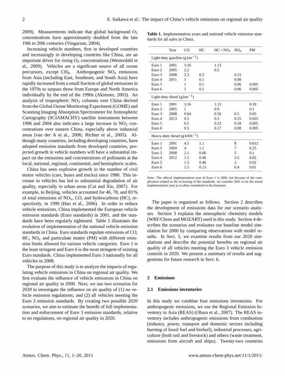
China has seen explosive growth in the number of civilmotor vehicles (cars, buses and trucks) since 1980. This in-crease in vehicles has led to substantial degradation of airquality, especially in urban areas (Cai and Xie, 2007). Forexample, in Beijing, vehicles accounted for 46, 78, and 83 %of total emissions of NOx, CO, and hydrocarbons (HC), re-spectively, in 1999 (Hao et al., 2006). In order to reducevehicle emissions, China implemented the European vehicleemission standards (Euro standards) in 2001, and the stan-dards have been regularly tightened. Table 1 illustrates theevolution of implementation of the national vehicle emissionstandards in China. Euro standards regulate emissions of CO,HC, NOx and particulate matter (PM) with different emis-sion limits allowed for various vehicle categories. Euro 1 isthe least stringent and Euro 6 is the most stringent of existingEuro standards. China implemented Euro 3 nationally for allvehicles in 2008.

The purpose of this study is to analyze the impacts of regu-lating vehicle emissions in China on regional air quality. Wefirst evaluate the influence of vehicle emissions in China onregional air quality in 2000. Next, we use two scenarios for2020 to investigate the influence on air quality of (1) no ve-hicle emission regulations; and (2) all vehicles meeting theEuro 3 emission standards. By creating two possible 2020scenarios, we aim to estimate the benefit of full implementa-tion and enforcement of Euro 3 emission standards, relativeto no regulations, on regional air quality in 2020.

Table 1. Implementation years and national vehicle emission stan-dards for all sales in China.

Year CO HC HC + NOx NOx PM

Light-duty gasoline (g km−1)

Euro 1Euro 2Euro 3Euro 4Euro 5Euro 6

2001200520082011

3.162.22.3111

0.20.10.10.1

1.130.5

0.150.080.060.06

0.0050.005

Light-duty diesel (g km−1)


2001200520082013

3.1610.640.50.50.5

1.130.90.560.30.230.17

0.50.250.180.08

0.180.10.050.0250.0050.005

Heavy-duty diesel (g kWh−1)


2001200420082012

4.542.11.51.51.5

1.11.10.660.460.460.13

8753.520.4

0.6120.250.10.020.020.01

Note: The official implementation year of Euro 1 is 2000, but because of the com-plication related to the re-issuing of the standards, we consider 2001 to be the actualimplementation year as is often considered in the literature.

The paper is organized as follows. Section 2 describesthe development of emissions data for our scenario analy-ses. Section 3 explains the atmospheric chemistry models(WRF/Chem and MOZART) used in this study. Section 4 de-scribes the scenarios and evaluates our baseline model sim-ulation for 2000 by comparing observations with model re-sults. In Sect. 5, we examine results from our 2020 sim-ulations and describe the potential benefits on regional airquality of all vehicles meeting the Euro 3 vehicle emissioncontrols in 2020. We present a summary of results and sug-gestions for future research in Sect. 6.

2 Emissions

2.1 Emissions inventories

In this study we combine four emissions inventories. Foranthropogenic emissions, we use the Regional Emission In-ventory in Asia (REAS) (Ohara et al., 2007). The REAS in-ventory includes anthropogenic emissions from combustion(industry, power, transport and domestic sectors includingburning of fossil fuel and biofuel), industrial processes, agri-culture (both soil and livestock) and others (waste treatment,emissions from aircraft and ships). Twenty-two countries

Atmos. Chem. Phys., 11, 1–20, 2011 www.atmos-chem-phys.net/11/1/2011/

E. Saikawa et al.: The impact of China’s vehicle emissions on regional air quality 3

40

1

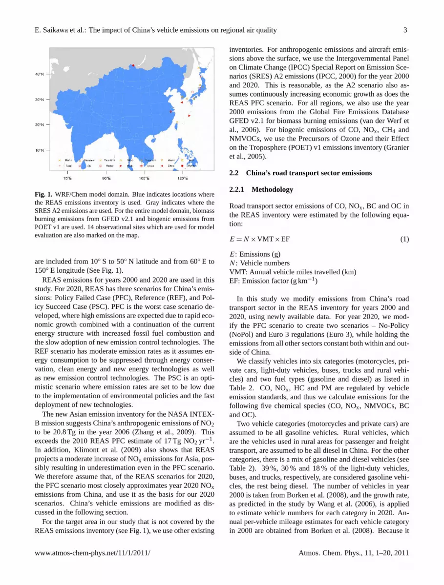
Fig. 1. WRF/Chem model domain. Blue indicates locations where the REAS emissions 2

inventory is used. Gray indicates where the SRES A2 emissions are used. For the entire 3

model domain, biomass burning emissions from GFED v2.1 and biogenic emissions from 4

POET v1 are used. 14 observational sites which are used for model evaluation are also 5

marked on the map. 6

7

Fig. 1. WRF/Chem model domain. Blue indicates locations wherethe REAS emissions inventory is used. Gray indicates where theSRES A2 emissions are used. For the entire model domain, biomassburning emissions from GFED v2.1 and biogenic emissions fromPOET v1 are used. 14 observational sites which are used for modelevaluation are also marked on the map.

are included from 10◦ S to 50◦ N latitude and from 60◦ E to150◦ E longitude (See Fig. 1).

REAS emissions for years 2000 and 2020 are used in thisstudy. For 2020, REAS has three scenarios for China’s emis-sions: Policy Failed Case (PFC), Reference (REF), and Pol-icy Succeed Case (PSC). PFC is the worst case scenario de-veloped, where high emissions are expected due to rapid eco-nomic growth combined with a continuation of the currentenergy structure with increased fossil fuel combustion andthe slow adoption of new emission control technologies. TheREF scenario has moderate emission rates as it assumes en-ergy consumption to be suppressed through energy conser-vation, clean energy and new energy technologies as wellas new emission control technologies. The PSC is an opti-mistic scenario where emission rates are set to be low dueto the implementation of environmental policies and the fastdeployment of new technologies.

The new Asian emission inventory for the NASA INTEX-B mission suggests China’s anthropogenic emissions of NO2to be 20.8 Tg in the year 2006 (Zhang et al., 2009). Thisexceeds the 2010 REAS PFC estimate of 17 Tg NO2 yr−1.In addition, Klimont et al. (2009) also shows that REASprojects a moderate increase of NOx emissions for Asia, pos-sibly resulting in underestimation even in the PFC scenario.We therefore assume that, of the REAS scenarios for 2020,the PFC scenario most closely approximates year 2020 NOxemissions from China, and use it as the basis for our 2020scenarios. China’s vehicle emissions are modified as dis-cussed in the following section.

For the target area in our study that is not covered by theREAS emissions inventory (see Fig. 1), we use other existing

inventories. For anthropogenic emissions and aircraft emis-sions above the surface, we use the Intergovernmental Panelon Climate Change (IPCC) Special Report on Emission Sce-narios (SRES) A2 emissions (IPCC, 2000) for the year 2000and 2020. This is reasonable, as the A2 scenario also as-sumes continuously increasing economic growth as does theREAS PFC scenario. For all regions, we also use the year2000 emissions from the Global Fire Emissions DatabaseGFED v2.1 for biomass burning emissions (van der Werf etal., 2006). For biogenic emissions of CO, NOx, CH4 andNMVOCs, we use the Precursors of Ozone and their Effecton the Troposphere (POET) v1 emissions inventory (Granieret al., 2005).

2.2 China’s road transport sector emissions

2.2.1 Methodology

Road transport sector emissions of CO, NOx, BC and OC inthe REAS inventory were estimated by the following equa-tion:

E = N ×VMT ×EF (1)

E: Emissions (g)N : Vehicle numbersVMT: Annual vehicle miles travelled (km)EF: Emission factor (g km−1)

In this study we modify emissions from China’s roadtransport sector in the REAS inventory for years 2000 and2020, using newly available data. For year 2020, we mod-ify the PFC scenario to create two scenarios – No-Policy(NoPol) and Euro 3 regulations (Euro 3), while holding theemissions from all other sectors constant both within and out-side of China.

We classify vehicles into six categories (motorcycles, pri-vate cars, light-duty vehicles, buses, trucks and rural vehi-cles) and two fuel types (gasoline and diesel) as listed inTable 2. CO, NOx, HC and PM are regulated by vehicleemission standards, and thus we calculate emissions for thefollowing five chemical species (CO, NOx, NMVOCs, BCand OC).

Two vehicle categories (motorcycles and private cars) areassumed to be all gasoline vehicles. Rural vehicles, whichare the vehicles used in rural areas for passenger and freighttransport, are assumed to be all diesel in China. For the othercategories, there is a mix of gasoline and diesel vehicles (seeTable 2). 39 %, 30 % and 18 % of the light-duty vehicles,buses, and trucks, respectively, are considered gasoline vehi-cles, the rest being diesel. The number of vehicles in year2000 is taken from Borken et al. (2008), and the growth rate,as predicted in the study by Wang et al. (2006), is appliedto estimate vehicle numbers for each category in 2020. An-nual per-vehicle mileage estimates for each vehicle categoryin 2000 are obtained from Borken et al. (2008). Because it

www.atmos-chem-phys.net/11/1/2011/ Atmos. Chem. Phys., 11, 1–20, 2011


Table 2. Vehicle numbers and annual mileage.

Vehicle category 2000(million)

2020(million)

Annualmileage(km)

Motorcycle 37.718 81.437 9000Private Car (Gasoline) 7.219 164.232 31 200Light-duty vehicle (Gasoline) 1.521 5.531 27 200Light-duty vehicle (Diesel)Bus (Gasoline)Bus (Diesel)Truck (Gasoline)Truck (Diesel)Rural vehicle (Diesel)

2.4110.3970.9290.5742.6599.645

8.7671.1912.7872.29610.63620.668

23 40034 00034 00030 00034 50017 500

Source: 2000 vehicle numbers and annual mileage come from Borken et al. (2008) andthe growth rates for 2020 from 2000 are taken from Wang et al. (2003).

is difficult to predict future driving patterns, we maintain thesame per-vehicle annual mileage for each vehicle categoryin 2020. This assumption for gasoline vehicles is most likelyan upper estimate, considering the estimated vehicle num-ber growth in private cars between 2000 and 2020. For thediesel vehicles, however, this number may increase in 2020.Therefore, CO and VOC emissions may be estimated higherdue to the bias in gasoline vehicles, whereas NOx and PMemissions may be estimated lower due to the bias in dieselvehicles. The values used for vehicle numbers and annualmileage for each vehicle category in 2000 and 2020 are sum-marized in Table 2.

2.2.2 Emission factors

Emission factors for 2000 are taken from Borken etal. (2008), and are listed in Table 3. For the sulphur contentof the fuel, we use the numbers that are used in REAS PFC. Itis 1200 ppm for gasoline and 1630 ppm for diesel (except forthe Northeast China where the sulphur content is 350 ppm).For 2020, we develop two scenarios based on clear policychoices, rather than making assumptions about technologicaldevelopments and fuel use. We develop a No-Policy (NoPol)scenario, which uses the same emission factors as in 2000;and the Euro 3 scenario, which uses emission factors takenfrom the Euro 3 standards for all vehicles except motorcy-cles and rural vehicles (these two classes of vehicles are as-sumed to remain at NoPol levels). Our 2020 NoPol and Euro3 simulations are identical except for their emission factors.Emissions allowed under Euro 3 standards are illustrated inTable 1. China nationally implemented the Euro 3 emissionstandards in 2008 for all categories of new vehicles exceptmotorcycles. Here we examine the air quality implicationsof perfect enforcement of these standards in China in 2020.

In trying to understand Asian emissions in 2006, Zhang etal. (2009) assumed that more than 85 % of gasoline vehicleswould meet Euro 1 or higher emission standards by 2006,and 60 % of gasoline vehicles would meet Euro 2 or Euro 3

emission standards. This rapid penetration of more stringentstandards in the 5 years since the first implementation of theEuro 1 standards in 2001 is a result of the rapidly growingtransport sector. Following their work, we assume that allvehicles will have control technologies that meet the Euro 3standards by 2020. We realize that some vehicles (especiallyin cities such as Beijing and Shanghai that adopted the Euro4 standards in 2008 and 2009, respectively) will meet morestringent vehicle emission standards, while old vehicles thatremain on the road will possibly not even meet the Euro 1standards. Since these standards are currently enforced onlyfor new vehicles, there are also uncertainties associated withemissions as vehicles age without sufficient in-use emissionregulations. To simplify the matter, however, we assume thaton average, Chinese vehicle emissions meet Euro 3 emissionstandards by 2020 in the Euro 3 scenario to quantify the airquality benefits of perfect implementation of these standards.Because there is no regulation adopted for motorcycle emis-sions and since it is not clear that rural vehicles would meetnational regulations, we assume that the emission factors formotorcycles and rural vehicles stay the same as they are inthe 2000 baseline simulation in both 2020 scenarios.

The emission factors for the Euro 3 scenario are calcu-lated using the Computer Programme to Calculate Emissionsfrom Road Transport (COPERT 4) model (European Envi-ronment Agency, 2009). COPERT 4 is a program that calcu-lates emission factors of all major air pollutants (CO, NOx,HC, PM2.5, NH3, SO2, heavy metals) for five vehicle cate-gories (passenger cars, light duty vehicles, heavy duty vehi-cles, mopeds and motorcycles) and six fuel categories (gaso-line, diesel, LPG, hybrid, CNG, and biodiesel), given specificparameters for: (1) driving condition (trip length, trip time,speed); (2) meteorology (minimum and maximum tempera-tures, Reid Vapour Pressure); and (3) fuel information (fuelspecifications such as sulphur content).

Studies have been conducted to analyze average vehiclespeeds in China. For example, Cai and Xie (2007) as-sumed 20, 40, and 80 km h−1 average speeds for urban, ru-ral, and freeway roads, respectively. Wang et al. (2008)conducted studies comparing driving parameters for differ-ent cities. The average speed in eleven cities is calculatedto be 29.1 km h−1, and thus we use 30 km h−1 for all travelin this study. The minimum and maximum monthly tem-peratures are calculated by taking the lowest and the highestaverage monthly temperatures from the 29 Chinese cities.We use 3.6◦C and 23.8◦C as the minimum and the max-imum monthly temperatures, respectively, and 64 kPa forReid Vapour Pressure (RVP), which measures the volatilityof gasoline. Sulphur content is taken from the Euro 3 stan-dard, which is 15 ppm for gasoline and 35 ppm for diesel.

The COPERT 4 program is designed for calculating ve-hicle emissions in Europe, and therefore does not calculateemission factors for heavy duty gasoline vehicles, as theyrarely exist in Europe. They are also not common in China,making up approximately 1 % of total vehicle population (see



Table 3. List of Emission Factors (g km−1).

Vehicle Type CO HC NOx PM BC OC

2000 & 2020 NoPol

MotorcyclePrivate Car (Gasoline)Light-duty vehicle (Gasoline)Light-duty vehicle (Diesel)Bus (Gasoline)Bus (Diesel)Truck (Gasoline)Truck (Diesel)Rural vehicle (Diesel)

12.98.621.8142.25.544.62.61.5

3.840.961.720.653.653.043.861.251.7

0.21.42.74.33.813.64121.1

0.20.150.210.280.351.010.350.620.2

0.0580.0430.0610.1590.1010.5730.1010.3520.114

0.0610.0460.0640.0510.1070.1820.1070.1120.036

2020 Euro 3

Private Car (Gasoline)Light-duty vehicle (Gasoline)Light-duty vehicle (Diesel)Bus (Gasoline)Bus (Diesel)Truck (Gasoline)Truck (Diesel)Rural vehicle (Diesel)

0.4943.5420.4072.12.2672.11.4131.5

0.0180.040.0910.080.4370.080.3061.7

0.0810.0971.0810.138.1750.135.3041.1

0.0010.0010.0580.060.180.060.1240.2

0.00030.00030.0330.0170.1020.0170.070.114

0.00030.00030.01050.01840.03250.01840.02240.036

Table 2), but to account for these, we used the vehicle emis-sion standards in Japan that most closely replicate Euro 3standards for these vehicle types. The emission factors forPM and NOx for heavy duty gasoline vehicles in the Euro 3scenario are taken from the 1994 PM/NOx Regulation. Forother species, the emission factors are taken from the 2000New Short Term Standard. The emission factors used in thisstudy are summarized in Table 3.

2.3 Regional emissions

For the three scenarios, total CO, NOx, BC, OC, andNMVOC emissions from China’s road transport sector alongwith emissions from four other sectors (domestic, othertransport, industry, and power plants) included in the REASinventory are shown in Fig. 2. All species except OC havethe lowest total emissions in the 2000 scenario and the high-est emissions in the 2020 NoPol scenario. In comparing theNoPol scenario with the 2000 baseline, China’s total CO,NOx, NMVOC, and BC emissions from all anthropogenicsources increase by 62 %, 178 %, 162 %, and 43 % (Table 4).The difference between the 2000 and the two 2020 scenariosis due not only to changes in the transport sector, but also inall other sectors.

OC emissions decrease in the 2020 scenarios because ofthe expected reduction of emissions in the residential sec-tor. OC emissions from the transport sector increase fromthe 2000 baseline to the two 2020 scenarios. For CO and BC,the largest increase from the 2000 to 2020 NoPol scenarios is

due to the increase in the gasoline, and diesel vehicle emis-sions, respectively. For NOx, we see a rapid increase in bothgasoline and diesel vehicle emissions, and at the same time,the emissions from power plant sources also increase signif-icantly. Table 4 illustrates that CO, NOx, NMVOC, BC andOC emissions from vehicles increase by 5.9, 4.9, 3.4, 2.3 and2.4 times in the 2020 NoPol scenario with respect to the 2000emissions, thereby increasing the proportion of emissions ofthese pollutants in China originating from vehicles.

There is seasonal variability in biomass burning and bio-genic emissions, but we do not account for such seasonal-ity in China’s vehicle emissions. The previous research inTianjin, China, Oliver (2008) has found that the summer COemissions were 18 % higher than those in spring. For NOxemissions, she found a 3 % increase in the summer, and therewas only a negligible difference for PM emissions. Consid-ering the seasonal variation in CO, it would be more realisticto include seasonality in our emissions. However, there is alack of data and Zhang et al. (2009) also notes that there isless seasonal cycle in vehicle emissions compared to othersources in China. We thus argue that, with a lack of data,including seasonality in emissions is not possible, but we be-lieve even without including this information we do not missan important feature of realistic vehicle emissions due to thesmall magnitude of the seasonal difference.

Combining with other emissions inventories we use fornon-anthropogenic sources, Fig. 3 provides the spatial distri-bution of the total CO, NOx, BC and OC monthly emissionsfor 2000 baseline, 2020 NoPol and 2020 Euro 3 scenarios.



41

1

2

3

Fig. 2. Total emissions from China’s six anthropogenic sectors (RD: Road Diesel, RG: Road 4

Gasoline, DOM: domestic, OTRA: other transport sector (airplanes, ships, etc), IND: 5

industry, and PP: power plants, EVAP: evaporative emissions, OTH: others – waste 6

treatment, surface emissions of aircraft and ships) in the three scenarios (2000, 2020NoPol, 7

and 2020Euro3) upper-left CO, upper-right NOx, middle-left BC, middle-right OC, lower-left 8

NMVOC (Gg yr-1). 9

10

Fig. 2. Total emissions from China’s six anthropogenic sectors (RD: Road Diesel, RG: Road Gasoline, DOM: domestic, OTRA: othertransport sector (airplanes, ships, etc), IND: industry, and PP: power plants, EVAP: evaporative emissions, OTH: others – waste treatment,surface emissions of aircraft and ships) in the three scenarios (2000, 2020NoPol, and 2020Euro3) upper-left CO, upper-right NOx, middle-leftBC, middle-right OC, lower-left NMVOC (Gg yr−1).

Here we provide the spatial distribution of emissions in Aprilfor the four species in the three scenarios. A large overallincrease in these emissions in the 2020 NoPol scenario rel-ative to the 2000 baseline is visible in Fig. 3. The increasein emissions from the 2000 baseline to 2020 NoPol is mostvisible for NOx emissions, whereas we see a decrease in theOC emissions in China except for the Beijing area. This iswhat we expect from the reduction in total emissions and theincrease in vehicle emissions of OC, as shown in Fig. 2.

For all species, there is a significant reduction of emis-sions from regulation of vehicle exhaust in 2020. Table 4shows that China’s total CO, NOx, NMVOCs, BC and OCemissions are reduced by 78 %, 74 %, 63 %, 63 % and 58 %,respectively, under the Euro 3 scenario relative to NoPol in2020. Due to this reduction in the road transport sector while

holding emissions from all other sources constant, the shareof vehicle emissions in China’s total emissions also decreasesignificantly in the Euro 3 scenario with respect to NoPol.For example, while the contribution of vehicles for total NOxemissions in NoPol is 46 %, it is reduced to only 18 % in theEuro 3 scenario. Similarly, the share is at least halved inall pollutants by perfect implementation of the Euro 3 emis-sion standards relative to no regulations. Emission reductionsfrom the NoPol to Euro 3 scenario are concentrated in citiesand the urban periphery, where there are vehicle emissions.Even though China’s total number of vehicles increases bya factor of 4.7 in 2020 with respect to 2000, CO, NOx, BC,OC, and NMVOC emissions from the road transport sectorin the Euro 3 scenario increase by only 1.5, 1.5, 1.2, 1.4, and1.6, respectively.



Table 4. Total anthropogenic emissions for each scenario in China(vehicle, total), Korea and Japan (kt year−1).

Species China(vehicle)

China(total)

Korea Japan

2000 baseline

CO 9279 127 461 4627 2661NOx 2574 11 745 1559 1959NMVOC 2125 13 249 1134 1880BC 105 1176 33 75OC 53 2594 57 44

2020 NoPol

CO 63 808 20 6856 6736 1846NOx 15 130 32 655 1955 1837NMVOC 9442 34 690 2231 2462BC 350 1676 34 36OC 180 2312 58 33

2020 Euro 3

CO 14 111 157 159 6736 1846NOx 3933 21 458 1955 1837NMVOC 3470 28 718 2231 2462BC 129 1456 34 36OC 75 2208 58 33

Some hotspots are also visible due to high biomass burn-ing emissions reported in the GFED v2.1 inventory. For ex-ample, a small fire is visible in Russia, close to Mongolia andKazakhstan border and also in Myanmar in April, as shownin Fig. 3. On these hotspots, there are high surface emissionsof all species, due to forest fires. It is important to note thatthe same forest fire hotspots are included in 2020 as in the2000 baseline, because the same emissions inventory is usedfor biomass burning in all scenarios.

3 The atmospheric chemistry transport models

In this study, we use the regional three-dimensional chemi-cal transport model Weather Research and Forecasting modelcoupled with Chemistry (WRF/Chem) v3.1.1, with initialand lateral chemical boundary conditions taken from a simu-lation of the global chemical transport Model for Ozone andRelated chemical Tracers (MOZART) v2.4.

3.1 The WRF/Chem model

We use the fully coupled “online” regional chemical trans-port model WRF/Chem version 3.1.1 (Grell et al., 2005,and references therein) in this study at a spatial resolutionof 40 km× 40 km with 31 vertical levels from the surfaceto 50 mb, the surface layer being approximately 12 m thick.The model domain is shown in Fig. 1, and covers the en-

42

1

2

3

4

Fig. 3. The monthly mean surface emissions of CO [kg km-2 month-1] (top), NOx [mol km-1 5

month-1] (second top), BC [g km-2 month-1] (second bottom) and OC [g km-2 month-1] 6

(bottom) in April, used in WRF/Chem for 2000 baseline, 2020 NoPol and 2020 Euro 3 7

scenarios. 8

Fig. 3. The monthly mean surface emissions of CO[kg km−2 month−1] (top), NOx [mol km−1 month−1] (second top),BC [g km−2 month−1] (second bottom) and OC [g km−2 month−1](bottom) in April, used in WRF/Chem for 2000 baseline, 2020NoPol and 2020 Euro 3 scenarios.

tire East Asia region with 199× 149 grid cells with a 40-km spacing, using a Lambert conformal map projection cen-tered on China at (32◦ N, 100◦ E). The grid-scale of 40 km,as compared to the much coarser grids used in global chemi-cal transport models, allows us to more precisely analyze theimpact of emission changes from the road transport sectoron air quality within Asia. Finer resolution is more able toresolve spatial heterogeneities in emission strengths and bet-ter simulates the non-linearities of ozone formation and lossprocesses (Jang et al., 1995).

In this study, the 2000 meteorological data are ob-tained from the National Centres for Environmental Pre-diction (NCEP) Global Forecast System final gridded anal-ysis datasets. Parameters include air temperature, surface



Table 5. List of WRF/Chem simulations.

Scenario Emissions in China Boundary

Vehicle emissions Other ConditionVehicle Emission emissionsnumber Factor

2000 2000 2000 2000 20002020 NoPol 2020 2000 2020PFC 2020 SRES A22020 Euro 3 2020 2020 Euro 3 2020PFC 2020 SRES A2

pressure, sea level pressure, geopotential height, tempera-ture, sea surface temperature, soil moisture, ice extent, snowdepth, relative humidity, u- and v-winds, etc. provided everysix hours.

The Regional Acid Deposition version 2 (RADM2) atmo-spheric chemical mechanism (Stockwell et al., 1990) is usedfor gas-phase chemistry. This mechanism is widely used inregional atmospheric chemistry models (for examples, seeLiu et al., 2008; Zhang et al., 2006). Aerosol chemistry isrepresented by the Model Aerosol Dynamics for Europe withthe Secondary Organic Aerosol Model (MADE/SORGAM)(Ackermann et al., 1998; Schell et al., 2001). It predictsthe mass of seven aerosol species (sulphate, ammonium, ni-trate, sea salt, organic carbon, secondary organic aerosols,and black carbon), using three log-normal aerosol modes(Aitken, accumulation and coarse). This mechanism doesnot include feedbacks of aerosol concentrations on the gas-phase chemistry via heterogeneous chemistry. Photolysisrates are obtained from the Fast-J photolysis scheme (Wildet al., 2000), and cumulus physics is parameterized using theGrell-3d ensemble cumulus scheme, an update of the Grell-Devenyi scheme (Grell and Devenyi, 2002).

3.2 MOZART-2

The global three-dimensional chemical transport model,MOZART version 2.4 (Horowitz, 2006; Horowitz et al.,2003) is used in this study to provide initial and lateralboundary conditions for 23 species in WRF/Chem (e.g. CO,NO, NO2, and O3). The horizontal resolution of MOZART-2is 2.8◦ latitude× 2.8◦ longitude, including 34 vertical levelsfrom the surface to 4.3 mb. Chemical and transport processesare driven by the National Center for Atmospheric Research(NCAR) MACCM3 meteorological fields for year 2000, us-ing the same simulations as in Horowitz (2006). The SRESA2 emissions for year 2000 or 2020 are used according to thescenarios in this study.

4 Simulations

4.1 Description of simulations

In order to simulate the present and potential future im-pact of emissions from China’s road transport sector on sur-face air quality in Asia, we performed the set of 3 simula-tions summarized in Table 5. Each scenario was run, usingWRF/Chem version 3.1.1, for four months (January, April,July and October). Considering the high computational de-mand of WRF/Chem, four months were selected to analyzeseasonal differences. For each one-month run, we used aspin-up of 2 weeks that was not included in the analysis.MOZART-2.4 was run for 2.5 years and the January, April,July and October of the last year of the simulation (year 2000for the 2000 simulation and year 2020 for the two 2020 simu-lations in all cases using year 2000 meteorology) was used asthe initial and lateral boundary conditions of the WRF/Chemmodel simulations. The same 2000 meteorology was usedfor all simulations, as our focus is to understand the impactthat regulatory controls of vehicle emissions have on regionalair quality. We do not include an analysis of the impact ofthese emission controls on dynamics or climate, and do notconsider inter-annual variability in air quality.

4.2 Comparison with measurements

WRF/Chem has been evaluated over the US (Grell et al.,2005) and Mexico City (Ying et al., 2009), but only a fewstudies have used it to examine the East Asian region (Linet al., 2010; Wang et al., 2010). This study is one of thefirst applications of the WRF/Chem model in the region,and we also use the newly modified REAS emissions inven-tory as well as new initial and lateral boundary conditionsfrom MOZART-2. We therefore evaluate our simulations forthe year 2000 with observations available to us from Japan,China, Korea, and Russia.

We calculate 24-h average O3 mixing ratios at each of thefollowing 9 measurement stations in Japan for the months ofJanuary, April, July and October in 2000 for the days thathave no missing values in the hourly measurements: Rishiri,Tappi, Sadoseki, Oki, Tsushima, Happo, Nikko, Hedo, and



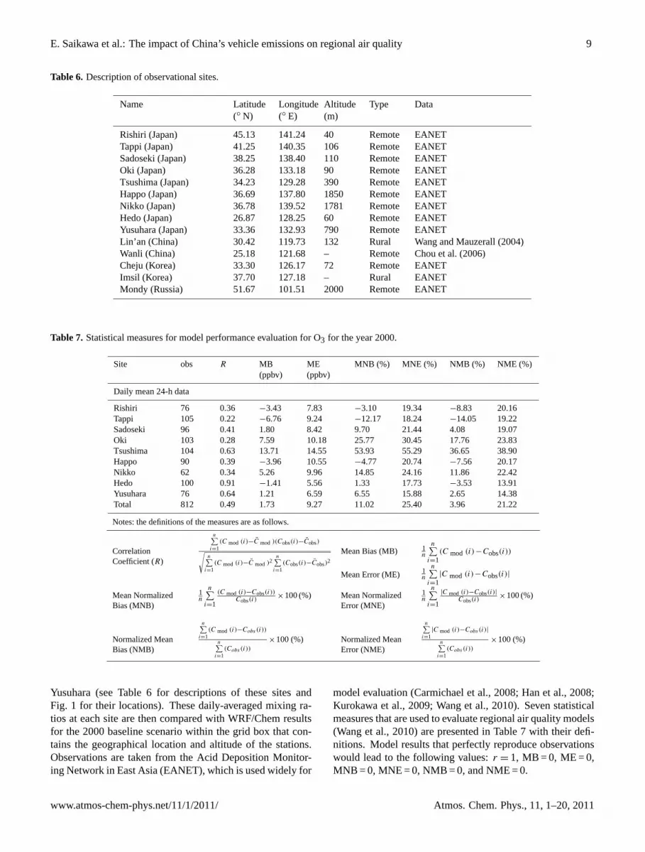
Table 6. Description of observational sites.

Name Latitude(◦ N)

Longitude(◦ E)

Altitude(m)

Type Data

Rishiri (Japan)Tappi (Japan)Sadoseki (Japan)Oki (Japan)Tsushima (Japan)Happo (Japan)Nikko (Japan)Hedo (Japan)Yusuhara (Japan)Lin’an (China)Wanli (China)Cheju (Korea)Imsil (Korea)Mondy (Russia)

45.1341.2538.2536.2834.2336.6936.7826.8733.3630.4225.1833.3037.7051.67

141.24140.35138.40133.18129.28137.80139.52128.25132.93119.73121.68126.17127.18101.51

40106110903901850178160790132–72–2000

RemoteRemoteRemoteRemoteRemoteRemoteRemoteRemoteRemoteRuralRemoteRemoteRuralRemote

EANETEANETEANETEANETEANETEANETEANETEANETEANETWang and Mauzerall (2004)Chou et al. (2006)EANETEANETEANET

Table 7. Statistical measures for model performance evaluation for O3 for the year 2000.

Site obs R MB(ppbv)

ME(ppbv)

MNB (%) MNE (%) NMB (%) NME (%)

Daily mean 24-h data

RishiriTappiSadosekiOkiTsushimaHappoNikkoHedoYusuharaTotal

7610596103104906210076812

0.360.220.410.280.630.390.340.910.640.49

−3.43−6.761.807.5913.71−3.965.26−1.411.211.73

7.839.248.4210.1814.5510.559.965.566.599.27

−3.10−12.179.7025.7753.93−4.7714.851.336.5511.02

19.3418.2421.4430.4555.2920.7424.1617.7315.8825.40

−8.83−14.054.0817.7636.65−7.5611.86−3.532.653.96

20.1619.2219.0723.8338.9020.1722.4213.9114.3821.22

Notes: the definitions of the measures are as follows.

CorrelationCoefficient (R)

n∑i=1

(C mod (i)−C mod )(Cobs(i)−Cobs)√n∑

i=1(C mod (i)−C mod )2

n∑i=1

(Cobs(i)−Cobs)2

Mean Bias (MB)

Mean Error (ME)

1n

n∑i=1

(C mod (i)−Cobs(i))

1n

n∑i=1

|C mod (i)−Cobs(i)|

Mean NormalizedBias (MNB)

1n

n∑i=1

(C mod (i)−Cobs(i))Cobs(i)

×100 (%) Mean NormalizedError (MNE)

1n

n∑i=1

|C mod (i)−Cobs(i)|Cobs(i)

×100 (%)

Normalized MeanBias (NMB)

n∑i=1

(C mod (i)−Cobs (i))

n∑i=1

(Cobs (i))

×100 (%) Normalized MeanError (NME)

n∑i=1

|C mod (i)−Cobs (i)|

n∑i=1

(Cobs (i))

×100 (%)

Yusuhara (see Table 6 for descriptions of these sites andFig. 1 for their locations). These daily-averaged mixing ra-tios at each site are then compared with WRF/Chem resultsfor the 2000 baseline scenario within the grid box that con-tains the geographical location and altitude of the stations.Observations are taken from the Acid Deposition Monitor-ing Network in East Asia (EANET), which is used widely for

model evaluation (Carmichael et al., 2008; Han et al., 2008;Kurokawa et al., 2009; Wang et al., 2010). Seven statisticalmeasures that are used to evaluate regional air quality models(Wang et al., 2010) are presented in Table 7 with their defi-nitions. Model results that perfectly reproduce observationswould lead to the following values:r = 1, MB = 0, ME = 0,MNB = 0, MNE = 0, NMB = 0, and NME = 0.



43

1

Fig. 4a. Comparison of observed (black) and simulated (red) daily mean O3 mixing ratios 2

(ppbv) at Rishiri, Tappi, Sadoseki, Oki, and Tsushima. Observed hourly values were taken 3

from EANET data for 2000 and averaged when there was no missing value in 24-hours. 4

Fig. 4a. Comparison of observed (black) and simulated (red) dailymean O3 mixing ratios (ppbv) at Rishiri, Tappi, Sadoseki, Oki, andTsushima. Observed hourly values were taken from EANET datafor 2000 and averaged when there was no missing value in 24-h.

44

1

Fig. 4b. Comparison of observed (black) and simulated (red) daily mean O3 mixing ratios 2

(ppbv) at, Happo, Nikko, Hedo, and Yusuhara. Observed hourly values were taken from 3

EANET data for 2000 and averaged when there was no missing value in 24-hours.4

Fig. 4b. Comparison of observed (black) and simulated (red)daily mean O3 mixing ratios (ppbv) at, Happo, Nikko, Hedo, andYusuhara. Observed hourly values were taken from EANET datafor 2000 and averaged when there was no missing value in 24-h.

In addition to the statistical analyses, we also compare themonthly average of the 12-h (08:00 a.m.–08:00 p.m.) and 24-h daily averages to the limited observational data available insimilar years (1999–2002) at six other non-Japanese sites:Lin’an and Wanli in China; Cheju and Imsil in South Korea;and Mondy in Russia. The description of these 6 sites issummarized in Table 6 and their locations are also indicatedin Fig. 1. We focus our evaluation on ozone (Sect. 4.2.1) andparticulate matter (Sect. 4.2.2).

4.2.1 Ozone

We compare the daily mean O3 mixing ratios of theWRF/Chem simulations with the daily mean of the hourlyobservations (excluding days when there were one or moremissing values at a given station) at the 9 EANET sites inJapan in Fig. 4. In Table 7 we present the statistical measuresevaluating model performance at the same sites. The stationsare all in remote areas that most likely represent backgroundO3 mixing ratios. Generally, the model reproduces the mea-sured O3 mixing ratios quite well. We find that MB is overallslightly positive, and the largest overestimation of the mea-surements takes place in Tsushima.

The correlation coefficient(R) of all the observed andmodelled O3 daily average mixing ratios for the four months(January, April, July and October) in 2000 is 0.49, with val-ues between 0.22 and 0.91, at individual sites. Combiningall the model results give an MB of 1.73 ppbv and ME of9.27 ppbv.

We also find seasonal differences in how well model re-sults represent observations. The largest discrepancies be-tween the model results and observations are found in July.The MNE is over 47.5 % and NME is 37 % for all the 207observations in July. These are much higher compared tothe values in other months, which have values lower than20 % for both MNE and NME. The site that contributes mostto this discrepancy is Tsushima, which lies on the Japanesecoast facing the Korean peninsula. When the statistical val-ues are calculated excluding Tsushima, the July MNE andNME values become 12 % and 37 %, respectively. One ofthe reasons for this discrepancy with observations at this sitein July is a possible overestimation of Korean emissions inthe REAS inventory. From the plot of O3 fluxes (appendix),it is evident that there is a large transport of O3 from the Ko-rean peninsula to the western coast of Japan in July. Korea’sCO, NOx, NMVOC emissions in the REAS inventory for theyear 2000 (see Table 4) are 5.1, 1.4, and 1.6 times larger thanthe official data, and high emissions from the Korean penin-sula are visible in the total CO, NOx, BC and OC emissionsshown in Fig. 3. Scaling the REAS inventory over Korea toagree with the official data may improve agreement betweenmodel results and observations.

In Fig. 5 we provide a comparison of the monthly averageof 12-h (08:00 a.m.–08:00 p.m.) and 24-h mean mixing ratiosof surface O3 calculated by WRF/Chem with observations in



45

1

Fig. 5. Comparison of observed (black) and simulated (red) monthly mean 12-hour daily 2

average (8am-8pm) O3 mixing ratios (ppbv) at Lin’an (China), comparison of observed and 3

simulated monthly mean 24-hour daily average mixing ratios (ppbv) at Wanli (China), Cheju 4

(Korea), Imsil (Korea), and Mondy (Russia). Observed values from Lin’an were taken from 5

Wang and Mauzerall (2004). The observations for Lin’an were made between August 1999 6

and July 2000. Observed values from Wanli were taken from Chou et al. (2006). Observed 7

values from Cheju, Imsil, and Mondy are taken from EANET data for 2002. 8

9

Fig. 5. Comparison of observed (black) and simulated (red) monthly mean 12-h daily average (08:00 a.m.–08:00 p.m.) O3 mixing ratios(ppbv) at Lin’an (China), comparison of observed and simulated monthly mean 24-h daily average mixing ratios (ppbv) at Wanli (China),Cheju (Korea), Imsil (Korea), and Mondy (Russia). Observed values from Lin’an were taken from Wang and Mauzerall (2004). Theobservations for Lin’an were made between August 1999 and July 2000. Observed values from Wanli were taken from Chou et al. (2006).Observed values from Cheju, Imsil, and Mondy are taken from EANET data for 2002.

China, South Korea and Russia in years between 1999 and2002. Here again, model results tend to overestimate ob-servations, but most of the model results lie within 10 ppbvof observations. At Lin’an, China, we find only small dis-crepancies in the model results with observations, and thehighest overestimation is found in January where model re-sults are 20 ppbv higher than the observed. This is similarto the seasonal biases found in other models (Kurokawa etal., 2009). On the other hand at Wanli, the model simu-lates observations within 10 ppbv. Lin’an is a rural site, andmay be influenced by local emissions from the Yangtze RiverDelta region, compared to the remote site of Wanli in Taiwan(Kurokawa et al., 2009). At Imsil, O3 is overestimated by30 ppbv in July, but at Cheju, with less influence from localemission sources, the simulated O3 mixing ratios are within10 ppbv of observations in the same month. Overall, our O3model results compare well with observations in remote ar-eas.

4.2.2 Particulate matter

Figure 6 displays the 24-h average PM2.5 observations andmodel results for the four months in 2000 (January, April,July, and October) at Rishiri and Oki stations in Japan. Ta-ble 8 provides the statistical measures for model perfor-mance. PM2.5 measurements are limited and they are onlyavailable at these two sites in Japan. The correlation co-efficient between the observed and modelled daily averagefor the four months (January, April, July and October) in2000 is 0.41 with 110 observations, and the MB of these to-tal observations is−5.41 µg m−3. In terms of error, ME is5.99 µg m−3, with MNE of 42.3 %.

Model results underestimate all observations at Rishiriwith MB of −1.48 µg m−3, but both MNB and MNE liewithin an acceptable range of−15.74 % and 15.74 %, respec-tively. Model results at Oki are also significantly underesti-mated most of the time, while occasionally slightly overes-timated. MB and ME for PM2.5 are as high as−8.14 and9.11 µg m−3, respectively.

46

1

Fig. 6. Comparison of observed (black) and simulated (red) daily mean PM2.5 concentrations 2

(µg m-3) at Rishiri and Oki. Observed hourly values were taken from EANET data for 2000 3

and averaged when there was no missing value in 24-hours. 4

5

Fig. 6. Comparison of observed (black) and simulated (red) dailymean PM2.5 concentrations (µg m−3) at Rishiri and Oki. Observedhourly values were taken from EANET data for 2000 and averagedwhen there was no missing value in 24-h.

There are several reasons for the general underestimationof PM2.5. First, dust emissions are not included, and onlyBC and OC are prescribed as primary PM2.5 emissions inWRF/Chem. Liu et al. (2009b) calculates that 43 % of totalPM2.5 surface concentrations in East Asia (including Mon-golia, China, Korean peninsula, and Japan) comes from dust.Zhang et al. (2009) also find that BC and OC only accountfor 42 % of primary PM2.5 emissions in China.

Zhang et al. (2009) further note the high uncertainty ofChina’s carbonaceous aerosol emissions, which may ex-plain why our model results agree better with observationsat Rishiri than at Oki. Rishiri is in the northern part ofHokkaido, and is more likely representative of backgroundconditions, while Oki is closer to the Asian continent, andis more likely to be affected by transport from China. Al-though both places have little local pollution, the impact ofprescribing less primary PM2.5 emissions is expected to havea greater influence on Oki, which is more affected by trans-ported pollution.

Second, the underestimate may also be caused by the ex-clusion of aqueous phase oxidation of SO2 by H2O2 and O3in the WRF/Chem model. Including only the gaseous phase



Table 8. Statistical measures for model performance evaluation for PM2.5 for the year 2000.

Site obs R MB(µg m−3)

ME(µg m−3)

MNB(%)

MNE(%)

NMB(%)

NME(%)

Daily mean 24-h data

Rishiri 45 0.43 −1.48 1.48 −15.74 15.74 −19.07 19.07Oki 65 0.45 −8.14 9.11 −46.70 60.69 −54.94 61.47

Total 110 0.41 −5.41 5.99 −34.03 42.30 −45.39 50.19

47

1

2

Fig. 7. The monthly mean surface O3 mixing ratios [ppbv] (top) and PM2.5 concentrations [µg 3

m-3] (bottom) in January, April, July and October, modelled by WRF/Chem for the 2000 4

baseline. 5

Fig. 7. The monthly mean surface O3 mixing ratios (ppbv) (top) andPM2.5 concentrations (µg m−3) (bottom) in January, April, July andOctober, modelled by WRF/Chem for the 2000 baseline.

oxidation of SO2 could significantly reduce the productionof sulphate, as aqueous phase oxidation could contribute ap-proximately 80 % of the sulphate production (McKeen et al.,2007; Barth et al., 2000; Koch et al., 1999).

Third, the RADM2 mechanism does not include monoter-pene photochemistry, and this may also contribute to the un-derestimation of PM2.5. Monoterpene photochemistry is aknown biogenic pathway for the formation of secondary or-ganic aerosol (SOA). An additional reason is that RADM2has limited oxidation pathways for anthropogenic VOCs,which may affect OC concentrations as anthropogenic VOCoxidation is important for SOA production (McKeen et al.,2007). All these factors likely contribute to underpredictionof PM2.5 in our WRF/Chem model results.

5 Scenario Simulations – surface air quality in 2000and 2020

5.1 Surface air quality in 2000

In Fig. 7 we present monthly average surface O3 mixing ra-tios and PM2.5 concentrations as calculated by WRF/Chemfor the year 2000 baseline scenario. The results show dif-ferences in seasonal and regional surface mixing ratios andconcentrations in the four months we have analyzed.

We simulate approximately 50 ppbv O3 in urban areaswith significant vehicle emissions, especially within North-east China. In July, O3 in excess of 100 ppbv is simulatedin the area near Busan, South Korea. This is most likely anoverestimate as found in Imsil in July (Sect. 4.2.1), mainlydue to the overestimated emissions. Also, due to high eleva-tion, surface O3 mixing ratios in the Tibetan plateau and theHimalayas are between 40–70 ppbv in most months.

PM2.5 has a lifetime of 1–2 weeks and, except for biomassburning, has similar emission patterns in the model through-out the year. Seasonal variability in surface concentrationsresults largely from changes in meteorology. We simulatelow surface concentrations in April and July, and high con-centrations in January and October. There is less precipita-tion in January and October in 2000, and this is one of thereasons for higher surface concentrations of PM2.5, due to



48

1

2

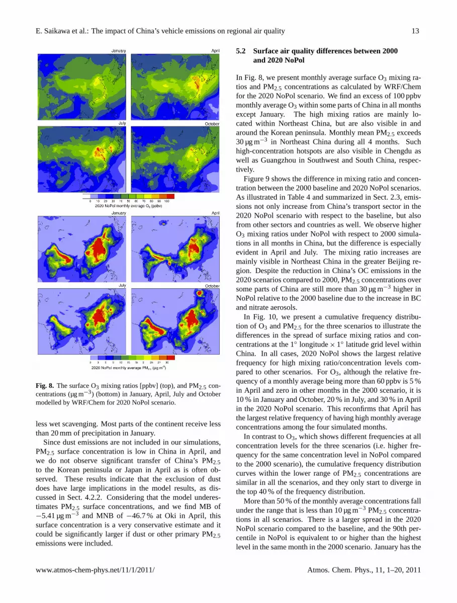
Fig. 8. The surface O3 mixing ratios [ppbv] (top), and PM2.5 concentrations [µg m-3] (bottom) 3

in January, April, July and October modelled by WRF/Chem for 2020 NoPol scenario. 4 Fig. 8. The surface O3 mixing ratios [ppbv] (top), and PM2.5 con-centrations (µg m−3) (bottom) in January, April, July and Octobermodelled by WRF/Chem for 2020 NoPol scenario.

less wet scavenging. Most parts of the continent receive lessthan 20 mm of precipitation in January.

Since dust emissions are not included in our simulations,PM2.5 surface concentration is low in China in April, andwe do not observe significant transfer of China’s PM2.5to the Korean peninsula or Japan in April as is often ob-served. These results indicate that the exclusion of dustdoes have large implications in the model results, as dis-cussed in Sect. 4.2.2. Considering that the model underes-timates PM2.5 surface concentrations, and we find MB of−5.41 µg m−3 and MNB of −46.7 % at Oki in April, thissurface concentration is a very conservative estimate and itcould be significantly larger if dust or other primary PM2.5emissions were included.

5.2 Surface air quality differences between 2000and 2020 NoPol

In Fig. 8, we present monthly average surface O3 mixing ra-tios and PM2.5 concentrations as calculated by WRF/Chemfor the 2020 NoPol scenario. We find an excess of 100 ppbvmonthly average O3 within some parts of China in all monthsexcept January. The high mixing ratios are mainly lo-cated within Northeast China, but are also visible in andaround the Korean peninsula. Monthly mean PM2.5 exceeds30 µg m−3 in Northeast China during all 4 months. Suchhigh-concentration hotspots are also visible in Chengdu aswell as Guangzhou in Southwest and South China, respec-tively.

Figure 9 shows the difference in mixing ratio and concen-tration between the 2000 baseline and 2020 NoPol scenarios.As illustrated in Table 4 and summarized in Sect. 2.3, emis-sions not only increase from China’s transport sector in the2020 NoPol scenario with respect to the baseline, but alsofrom other sectors and countries as well. We observe higherO3 mixing ratios under NoPol with respect to 2000 simula-tions in all months in China, but the difference is especiallyevident in April and July. The mixing ratio increases aremainly visible in Northeast China in the greater Beijing re-gion. Despite the reduction in China’s OC emissions in the2020 scenarios compared to 2000, PM2.5 concentrations oversome parts of China are still more than 30 µg m−3 higher inNoPol relative to the 2000 baseline due to the increase in BCand nitrate aerosols.

In Fig. 10, we present a cumulative frequency distribu-tion of O3 and PM2.5 for the three scenarios to illustrate thedifferences in the spread of surface mixing ratios and con-centrations at the 1◦ longitude× 1◦ latitude grid level withinChina. In all cases, 2020 NoPol shows the largest relativefrequency for high mixing ratio/concentration levels com-pared to other scenarios. For O3, although the relative fre-quency of a monthly average being more than 60 ppbv is 5 %in April and zero in other months in the 2000 scenario, it is10 % in January and October, 20 % in July, and 30 % in Aprilin the 2020 NoPol scenario. This reconfirms that April hasthe largest relative frequency of having high monthly averageconcentrations among the four simulated months.

In contrast to O3, which shows different frequencies at allconcentration levels for the three scenarios (i.e. higher fre-quency for the same concentration level in NoPol comparedto the 2000 scenario), the cumulative frequency distributioncurves within the lower range of PM2.5 concentrations aresimilar in all the scenarios, and they only start to diverge inthe top 40 % of the frequency distribution.

More than 50 % of the monthly average concentrations fallunder the range that is less than 10 µg m−3 PM2.5 concentra-tions in all scenarios. There is a larger spread in the 2020NoPol scenario compared to the baseline, and the 90th per-centile in NoPol is equivalent to or higher than the highestlevel in the same month in the 2000 scenario. January has the



49

1

2

Fig. 9. Comparison of 2020 NoPol and 2000 baseline (2020NoPol – 2000 baseline) surface O3 3

mixing ratios [ppbv] (top), and PM2.5 concentrations [µg m-3] (bottom) in January, April, July 4

and October modelled by WRF/Chem. 5

Fig. 9. Comparison of 2020 NoPol and 2000 baseline (2020NoPol–2000 baseline) surface O3 mixing ratios [ppbv] (top), and PM2.5concentrations (µg m−3) (bottom) in January, April, July and Octo-ber modelled by WRF/Chem.

highest concentration levels and 5 % of the grid cells withinChina in the 2020 NoPol scenario have a January monthlyaverage concentration higher than 50 µg m−3.

It is also important to note that populated areas are whereO3 and PM2.5 concentrations are high. This has an importantimplication for adverse health impacts, as the reduction ofthese air pollutants lead to reduced human exposure.

5.3 Surface air quality differences between 2020 NoPoland 2020 Euro3

In Fig. 11, we present monthly average surface concentra-tions of O3 and PM2.5 as calculated by WRF/Chem for the2020 Euro 3 scenario. In contrast to NoPol, far fewer ar-

eas in China have extremely high surface O3 mixing ratios,and most places have a monthly average below 70 ppbv in allmonths. As for PM2.5, although the area is considerably re-duced compared to the NoPol scenario, some parts of North-east China still shows monthly average surface concentra-tions above 30 µg m−3.

Figure 12 shows the difference in monthly average sur-face O3 mixing ratios and PM2.5 concentrations between thetwo 2020 scenarios. In contrast to the difference betweenthe 2000 and 2020 NoPol scenarios (Fig. 9), the differencebetween the two 2020 scenarios are due only to the reduc-tion in vehicle emissions by implementing the Euro 3 regula-tions; all other emissions kept the same. Therefore, the two2020 scenarios show similar trends, but the concentrationsare much higher within urban regions of China in the NoPolscenario due to greater vehicle emissions.

As the lifetime of O3 is approximately a month and be-cause of the non-linearities of O3 production, the implemen-tation of Euro 3 standards in China leads to a regional re-duction of surface O3. The largest difference in O3 mix-ing ratios between the two scenarios is found in East China,where there are projected to be a large number of vehicles.Maximum reductions in O3 mixing ratios within China fromNoPol to Euro 3 are 11, 15, 21, and 22 ppbv in January, April,July, and October, respectively.

The reduction of PM2.5 in the Euro 3 scenario as com-pared with NoPol is also seen widely in East China. Inthe Northeast, a reduction of more than 10 µg m−3 is occa-sionally found with the highest reductions being 31, 14, 15,and 26 µg m−3 for January, April, July, and October, respec-tively. Considering that the maximum concentration in the2000 baseline simulation is 37 µg m−3 in January, this is asignificant improvement in air quality.

Depending on the season, we also see a regional impactof China’s implementation of the Euro 3 vehicle emissionstandards, relative to no regulations. For example in Jan-uary, the Korean peninsula, Southeast Asia, and Japan ex-cept Hokkaido experience a reduction of 2–3 ppbv or moreof O3 under the Euro 3 scenario relative to NoPol. In April,the Korean peninsula sees 6–7 ppbv O3 reduction and evenHokkaido benefits from a 1–2 ppbv reduction. Similarly, areduction of more than 10 µg m−3 is also visible in PM2.5monthly average concentrations over the Korean peninsulain these months. In July and October, reductions are mainlyfound within China. Still, the Korean peninsula and Japanclearly benefit from China’s implementation of the Euro 3emission standards.

In Fig. 10, we find that there is a visible difference in thecumulative frequency distribution of O3 and PM2.5 monthlyaverage for the two 2020 scenarios within China. For exam-ple, whereas 36 % of the grid cells within China in the NoPolscenario have more than 60 ppbv O3 monthly average mixingratio in April, the relative frequency is reduced to less than24 % with the Euro 3 emission regulations. Similarly, therelative frequency of a grid cell having more than 30 µg m−3



Fig. 10.Cumulative frequency distribution of China’s surface O3 mixing ratios (ppbv), and PM2.5 concentrations (µg m−3) in January, April,July and October modelled by WRF/Chem.

PM2.5 monthly average concentration decreases from 13 %in the NoPol scenario to 6 % in the Euro 3 scenario in Jan-uary.

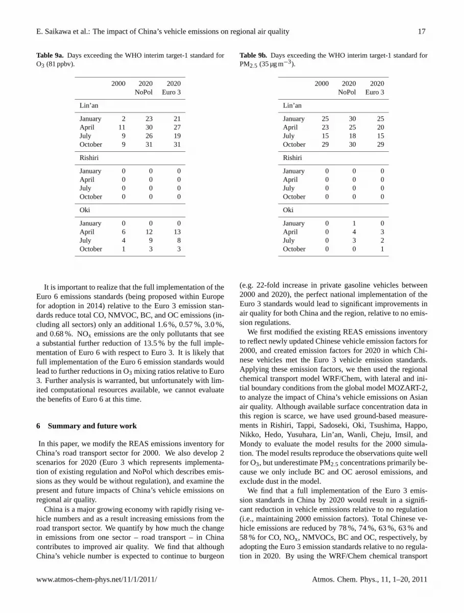
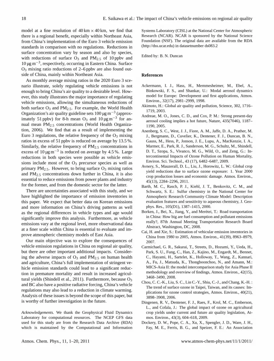
Simply by implementing the vehicle emission standards,China is more likely able to meet the World Health Organi-zation’s 8-h O3 interim target-1 standards of 160 µg m−3 (ap-proximately 81 ppbv) and annual mean PM2.5 interim target-1 standards of 35 µg m−3 (World Health Organization, 2006).

In Table 9, we present the number of days where the 8-haverage O3 and PM2.5 in Lin’an, Rishiri and Oki for eachscenario is above 81 ppbv and 35 µg m−3, respectively. Theimportant finding is that by implementing the Euro 3 emis-sion standards in 2020, Lin’an is able to at least keep, if notlessen the exceedance level of PM2.5 as in 2000. AlthoughO3 mixing ratios increase quite rapidly in 2020 due to theincreased emissions in all sectors, we find that implementing



51

1

2

Fig. 11. The surface O3 mixing ratios [ppbv] (top) and PM2.5 concentrations [µg m-3] (bottom) 3

in January April, July and October modelled by WRF/Chem for 2020 Euro 3 scenario. 4 Fig. 11. The surface O3 mixing ratios [ppbv] (top) and PM2.5 con-centrations (µg m−3) (bottom) in January April, July and Octobermodelled by WRF/Chem for 2020 Euro 3 scenario.

the Euro 3 standards leads to a reduction of 7 exceedancedays in July in Lin’an. Under Euro 3 the maximum 8-h O3and PM2.5 average at Oki is also 1–3 ppbv and 3–7 µg m−3

lower, respectively, than under NoPol. However, there arestill many exceedance days in China even under the Euro 3scenario (Table 9). These results illustrate that regulating ve-hicle emissions alone does not achieve targeted air quality inChina, despite the significant improvement. Further regula-tions in other sectors on top of the implementation of vehicleemission standards are essential to achieve this goal.

In summary, we find clear benefits of reducing vehicleemissions in China from this study. Full implementation ofEuro 3 regulations in China result in the largest reductionsin O3 and PM2.5 surface concentrations in October and Jan-uary, respectively. In addition, there are large reductions in

Fig. 12.Comparison of 2020 NoPol and 2020 Euro 3 (2020 NoPol–2020 Euro 3) surface O3 mixing ratios (ppbv) (top), and PM2.5 con-centrations (µg m−3) (bottom) in January, April, July and Octobermodelled by WRF/Chem.

April and July for surface O3, as seen in Fig. 10. Vehicleemission regulations lead to significant reductions in both O3and PM2.5, because stringent vehicle emission regulations re-quire reductions in the emissions of primary PM2.5, and theO3 precursor species – CO, NOx, and NMVOCs. The threelargest surface concentration reductions are seen in Beijing,Shanghai, and Guangzhou areas (see Fig. 12), where we findlarge vehicle emissions (Fig. 3). Although the road transportsector is responsible for a small fraction of BC and OC emis-sions (Fig. 2), with Euro 3 regulations we find significantPM2.5 surface concentration reductions also due to less for-mation of nitrate aerosols from reduced NOx emissions anddue to the reduced availability of excess NH4.



Table 9a. Days exceeding the WHO interim target-1 standard forO3 (81 ppbv).

2000 2020 2020NoPol Euro 3

Lin’an

January 2 23 21April 11 30 27July 9 26 19October 9 31 31

Rishiri


Oki


It is important to realize that the full implementation of theEuro 6 emissions standards (being proposed within Europefor adoption in 2014) relative to the Euro 3 emission stan-dards reduce total CO, NMVOC, BC, and OC emissions (in-cluding all sectors) only an additional 1.6 %, 0.57 %, 3.0 %,and 0.68 %. NOx emissions are the only pollutants that seea substantial further reduction of 13.5 % by the full imple-mentation of Euro 6 with respect to Euro 3. It is likely thatfull implementation of the Euro 6 emission standards wouldlead to further reductions in O3 mixing ratios relative to Euro3. Further analysis is warranted, but unfortunately with lim-ited computational resources available, we cannot evaluatethe benefits of Euro 6 at this time.

6 Summary and future work

In this paper, we modify the REAS emissions inventory forChina’s road transport sector for 2000. We also develop 2scenarios for 2020 (Euro 3 which represents implementa-tion of existing regulation and NoPol which describes emis-sions as they would be without regulation), and examine thepresent and future impacts of China’s vehicle emissions onregional air quality.

China is a major growing economy with rapidly rising ve-hicle numbers and as a result increasing emissions from theroad transport sector. We quantify by how much the changein emissions from one sector – road transport – in Chinacontributes to improved air quality. We find that althoughChina’s vehicle number is expected to continue to burgeon

Table 9b. Days exceeding the WHO interim target-1 standard forPM2.5 (35 µg m−3).

2000 2020 2020NoPol Euro 3

Lin’an


Rishiri


Oki


(e.g. 22-fold increase in private gasoline vehicles between2000 and 2020), the perfect national implementation of theEuro 3 standards would lead to significant improvements inair quality for both China and the region, relative to no emis-sion regulations.

We first modified the existing REAS emissions inventoryto reflect newly updated Chinese vehicle emission factors for2000, and created emission factors for 2020 in which Chi-nese vehicles met the Euro 3 vehicle emission standards.Applying these emission factors, we then used the regionalchemical transport model WRF/Chem, with lateral and ini-tial boundary conditions from the global model MOZART-2,to analyze the impact of China’s vehicle emissions on Asianair quality. Although available surface concentration data inthis region is scarce, we have used ground-based measure-ments in Rishiri, Tappi, Sadoseki, Oki, Tsushima, Happo,Nikko, Hedo, Yusuhara, Lin’an, Wanli, Cheju, Imsil, andMondy to evaluate the model results for the 2000 simula-tion. The model results reproduce the observations quite wellfor O3, but underestimate PM2.5 concentrations primarily be-cause we only include BC and OC aerosol emissions, andexclude dust in the model.

We find that a full implementation of the Euro 3 emis-sion standards in China by 2020 would result in a signifi-cant reduction in vehicle emissions relative to no regulation(i.e., maintaining 2000 emission factors). Total Chinese ve-hicle emissions are reduced by 78 %, 74 %, 63 %, 63 % and58 % for CO, NOx, NMVOCs, BC and OC, respectively, byadopting the Euro 3 emission standards relative to no regula-tion in 2020. By using the WRF/Chem chemical transport



model at a fine resolution of 40 km× 40 km, we find thatthere is a regional benefit, especially within Northeast Asia,from China’s implementation of the Euro 3 vehicle emissionstandards in comparison with no regulations. Reductions insurface concentration vary by season and also by species,with reductions of surface O3 and PM2.5 of 10 ppbv and10 µg m−3, respectively, occurring in Eastern China. SurfaceO3 mixing ratio reductions of 2–6 ppbv are also found out-side of China, mainly within Northeast Asia.

As monthly average mixing ratios in the 2020 Euro 3 sce-nario illustrate, solely regulating vehicle emissions is notenough to bring China’s air quality to a desirable level. How-ever, this study illustrates the major importance of regulatingvehicle emissions, allowing the simultaneous reductions ofboth surface O3 and PM2.5. For example, the World HealthOrganization’s air quality guideline sets 100 µg m−3 (approx-imately 51 ppbv) for 8-h mean O3 and 10 µg m−3 for an-nual mean PM2.5 concentrations (World Health Organiza-tion, 2006). We find that as a result of implementing theEuro 3 regulations, the relative frequency of the O3 mixingratios in excess of 51 ppbv is reduced on average by 13.5 %.Similarly, the relative frequency of PM2.5 concentrations inexcess of 10 µg m−3 is reduced on average by 4.5 %. Largereductions in both species were possible as vehicle emis-sions include most of the O3 precursor species as well asprimary PM2.5. However, to bring surface O3 mixing ratiosand PM2.5 concentrations down further in China, it is alsoessential to reduce emissions from power plants and industryfor the former, and from the domestic sector for the latter.

There are uncertainties associated with this study, and wehave highlighted the importance of emission inventories inthis paper. We expect that better data on Korean emissionsand more information on China’s driving patterns as wellas the regional differences in vehicle types and age wouldsignificantly improve this analysis. Furthermore, as vehicleemissions vary at the regional level, more observational dataat a finer scale within China is essential to evaluate and im-prove atmospheric chemistry models of East Asia.

Our main objective was to explore the consequences ofvehicle emission regulations in China on regional air quality,but there are other important additional impacts. Consider-ing the adverse impacts of O3 and PM2.5 on human healthand agriculture, China’s full implementation of stringent ve-hicle emission standards could lead to a significant reduc-tion in premature mortality and result in increased agricul-tural yields (Shindell et al., 2011). Furthermore, because O3and BC also have a positive radiative forcing, China’s vehicleregulations may also lead to a reduction in climate warming.Analysis of these issues is beyond the scope of this paper, butis worthy of further investigation in the future.

Acknowledgements.We thank the Geophysical Fluid DynamicsLaboratory for computational resources. The NCEP GFS dataused for this study are from the Research Data Archive (RDA)which is maintained by the Computational and Information

Systems Laboratory (CISL) at the National Center for AtmosphericResearch (NCAR). NCAR is sponsored by the National ScienceFoundation (NSF). The original data are available from the RDA(http://dss.ucar.edu) in datasetnumber ds083.2

Edited by: B. N. Duncan

References

Ackermann, I. J., Hass, H., Memmesheimer, M., Ebel, A.,Binkowski, F. S., and Shankar, U.: Modal aerosol dynamicsmodel for Europe: Development and first applications, Atmos.Environ., 32(17), 2981–2999, 1998.

Akimoto, H.: Global air quality and pollution, Science, 302, 1716–1719, 2003.

Andreae, M. O., Jones, C. D., and Cox, P. M.: Strong present-dayaerosol cooling implies a hot future, Nature, 435(7046), 1187–1190, 2005.

Anenberg, S. C., West, J. J., Fiore, A. M., Jaffe, D. A., Prather, M.J., Bergmann, D., Cuvelier, K., Dentener, F. J., Duncan, B. N.,Gauss, M., Hess, P., Jonson, J. E., Lupu, A., MacKenzie, I. A.,Marmer, E., Park, R. J., Sanderson, M. G., Schultz, M., Shindell,D. T., Szopa, S., Vivanco, M. G., Wild, O., and Zeng, G.: In-tercontinental Impacts of Ozone Pollution on Human Mortality,Environ. Sci. Technol., 43 (17), 6482–6487, 2009.

Avnery, S., Mauzerall, D. L., Liu, J., Horowitz, L. W.: Global cropyield reductions due to surface ozone exposure: 1. Year 2000crop production losses and economic damage. Atmos. Environ.,45(13), 2284–2296, 2011.

Barth, M. C., Rasch, P. J., Kiehl, J. T., Benkovitz, C. M., andSchwartz, S. E.: Sulfur chemistry in the National Center forAtmospheric Research Community Climate Model: Descriptionevaluation features and sensitivity to aqueous chemistry, J. Geo-phys. Res., 105(D1), 1387–1415, 2000.

Borken, J., Bei, X., Jiang, Y., and Meretei, T.: Road transportationin China: How big are fuel consumption and pollutant emissionsreally?, 87th Annual Meeting Transportation Research BoardAbstract, Washington, DC, 2008.

Cai, H. and Xie, S.: Estimation of vehicular emission inventories inChina from 1980 to 2005, Atmos. Environ., 41(39), 8963–8979,2007.

Carmichael, G. R., Sakurai, T., Streets, D., Hozumi, Y., Ueda, H.,Park, S. U., Fung, C., Han, Z., Kajino, M., Engardt, M., Bennet,C., Hayami, H., Sartelet, K., Holloway, T., Wang, Z., Kannari,A., Fu, J., Matsuda, K., Thongboonchoo, N., and Amann, M.:MICS-Asia II: the model intercomparison study for Asia Phase IImethodology and overview of findings, Atmos. Environ., 42(15),3468–3490, 2008.

Chou, C. C.-K., Liu, S. C., Lin C.-Y., Shiu, C.-J., and Chang, K.-H. :The trend of surface ozone in Taipei, Taiwan, and its causes: Im-plications for ozone control strategies, Atmos. Environ., 40(21),3898–3908, 2006.

Dingenen, R. V., Dentener, F. J., Raes, F., Krol, M. C., Emberson,L., and Cofala, J.: The global impact of ozone on agriculturalcrop yields under current and future air quality legislation, At-mos. Environ., 43(3), 604–618, 2009.

Dockery, D. W., Pope, C. A., Xu, X., Spengler, J. D., Ware, J. H.,Fay, M. E., Ferris, B. G., and Speizer, F. E.: An Association


http://dss.ucar.edu


between Air Pollution and Mortality in Six US Cities, N. Engl. J.Med., 329(24), 1753–1759, 1993.

European Environment Agency: EMEP/CORINAIR AtmosphericEmissions Inventory Guidebook – 2009, Copenhagen, 2009.

Fiore, A. M., Dentener, F. J, Wild, O., Cuvelier, C., Schultz, M. G.,Hess, P., Textor, C., Schulz, M., Doherty, R. M., Horowitz, L.W., MacKenzie, I. A., Sanderson, M. G., Shindell, D. T., Steven-son, D. S., Szopa, S., Van Dingenen, R., Zeng, G., Atherton, C.,Bergmann, D., Bey, I., Carmichael, G., Collins, W. J., Duncan,B. N., Faluvegi, G., Folberth, G., Gauss, M., Gong, S., Hauglus-taine, D., Holloway, T., Isaksen, I. S. A., Jacob, D. J., Jonson,J. E., Kaminski, J. W., Keating, T. J., Lupu, A., Marmer, E.,Montanaro, V., Park, R. J., Pitari, G., Pringle, K. J., Pyle, J. A.,Schroeder, S., Vivanco, M. G., Wind, P., Wojcik, G., Wu, S.,and Zuber, A.: Multimodel estimates of intercontinental source-receptor relationships for ozone pollution, J. Geophys. Res., 114,D04301,doi:10.1029/2008JD010816, 2009.

Forster, P., Ramaswamy, V., Artaxo, P., Berntsen, T. Betts, R., Fa-hey, D. W., Haywood, J., Lean, J., Lowe, D. C., Myhre, G.,Nganga, J., Prinn, R., Raga, G., Schulz, M. and Van Dorland, R.:Changes in atmospheric constituents and in radiative forcing, in:Climate Change 2007: The Physical Science Basis. Contributionof Working Group I to the 4th, Assessment Report of the inter-governmental Panel on Climate Change, Cambridge UniversityPress, 2007.

Granier, C., Lamarque, J. F., Mieville, A., Muller, J. F., Olivier,J., Orlando, J., Peters, J., Petron, G., Tyndall, G., and Wallens,S.: POET, a database of surface emissions of ozone precursors,available at: http://www.aero.jussieu.fr/projet/ACCENT/POET.php, 2005.

Grell, G. A. and Devenyi, G.: A generalized approach toparameterizing convection combining ensemble and data as-similation techniques, Geophys. Res. Lett., 29(14), 1693,doi:10.1029/2002GL015311, 2002.

Grell, G. A., Peckham, S. E., Schmitz, R., McKeen, S. A., Frost, G.,Skamarock, W. C., and Eder, B.: Fully coupled “online” chem-istry with the WRF model, Atmos. Environ., 39(37), 6957–6975,2005.

Han, Z., Sakurai, T., Ueda, H., Carmichael, G. R., Streets, D.,Hayami, H., Wang, Z., Holloway, T., Engardt, M., Hozumi,Y., Park, S. U., Kajino, M., Sartelet, K., Fung, C., Bennet, C.,Thongboonchoo, N., Tang, Y., Chang, A., Matsuda, K., andAmann, M.: MICS-Asia II: model intercomparison and evalu-ation of ozone and relevant species, Atmos. Environ., 42(14),3491–3509, 2008.

Hao, J., Hu, J., and Lixin, F.: Controlling vehicular emissions inBeijing during the last decade, Transportation Research Part A,40, 639–651, 2006.

Horowitz, L. W.: Past, present, and future concentrations of tro-pospheric ozone and aerosols: Methodology, ozone evaluation,and sensitivity to aerosol wet removal, J. Geophys. Res., 111,D22211,doi:10.1029/2005JD006937, 2006.

Horowitz, L. W., Walters, S., Mauzerall, D. L., Emmons, L. K.,Rasch, P. J., Granier, C., Tie, X., Lamarque, J.-F., Schultz, M.G., Tyndall, G. S., Orlando, J. J., andn Brasseur, G. P.: A globalsimulation of tropospheric ozone and related tracers: Descrip-tion and evaluation of MOZART, version 2, J. Geophys. Res.,108(D24), 4784,doi:10.1029/2002JD002853, 2003.

Intergovernmental Panel on Climate Change (IPCC): Special Re-

port on Emissions Scenarios: A Special Report of WorkingGroup III of the Intergovernmental Panel on Climate Change,Cambridge University Press, Cambridge, UK, 2000.

Jang, J-C. C., Jeffries, H. E., Byun, D., and Pleim, J. E.: Sen-sitivity of ozone to model grid resolution – I. Application ofhigh-resolution regional acid deposition model, Atmos. Environ.,29(21), 3085–3100, 1995.

Klimont, Z., Cofala, J., Xing, J., Wei, W., Zhang, C., Wang, S., Ke-jun, J., Bhandari, P., Mathur, R., Purohit, P., Rafaj, P., Chambers,A., and Amann, M.: Projections of SO2, NOx and carbonaceousaerosols emissions in Asia, Tellus B, 61, 602–617, 2009.

Koch, D., Jacob, D., Tegen, I., Rind, D., and Chin, M.: Tropo-spheric sulphur simulation and sulphate direct radiative forcingin the Goddard Institute for Space Studies general circulationmodel, J. Geophys. Res., 104(D19), 23799–23822, 1999.

Kurokawa, J., Ohara, T., Uno, I., Hayasaki, M., and Tanimoto, H.:Influence of meteorological variability on interannual variationsof springtime boundary layer ozone over Japan during 1981-2005, Atmos. Chem. Phys., 9, 6287–6304,doi:10.5194/acp-9-6287-2009, 2009.

Levy, J. I., Carrothers, T. J., Tuomisto, J. T., Hammitt, J. K., andEvans, J. S.: Assessing the public health benefits of reducedozone concentrations, Environ. Health Persp., 109(12), 1215-1226, 2001.

Lin, M., Holloway, T., Carmichael, G. R., and Fiore, A. M.: Quan-tifying pollution inflow and outflow over East Asia in springwith regional and global models, Atmos. Chem. Phys., 10, 4221–4239,doi:10.5194/acp-10-4221-2010, 2010.

Liu, C.-M., Yeh, M.-T., Paul, S., Lee, Y.-C., Jacob, D. J., Fu, M.,Woo, J.-H., Carmichael, G. R., and Streets, D. G.: Effect of an-thropogenic emissions in East Asia on regional ozone levels dur-ing spring cold continental outbreaks near Taiwan: A case study,Environ. Modelling. Software., 23(5), 579–591, 2008.

Liu, J., Mauzerall, D. L., and Horowitz, L. W.: Evaluating inter-continental transport of fine aerosols: (2) Global Health Impacts,Atmos. Environ., 43(28), 4339–4347, 2009a.

Liu, J., Mauzerall, D. L., Horowitz, L. W., Ginoux, P., and Fiore, A.M.: Evaluating inter-continental transport of fine aerosols: (1)Methodology, global aerosol distribution and optical depth, At-mos. Environ., 43(28), 4327–4338, 2009b.

McKeen, S., Chung, S. H., Wilczak, J., Grell, G., Djalalova,I., Peckham, S., Gong, W., Bouchet, V., Moffet, R., Tang,Y., Carmichael, G. R., Mathur, R., and Yu, S.: Evaluationof several PM2.5 forecast models using data collected duringthe ICARTT/NEAQS 2004 field study, J. Geophys. Res., 112,D10S20,doi:10.1029/2006JD007608, 2007.

Ohara, T., Akimoto, H., Kurokawa, J., Horii, N., Yamaji, K.,Yan, X., and Hayasaka, T.: An Asian emission inventory ofanthropogenic emission sources for the period 19802020, At-mos. Chem. Phys., 7, 4419–4444,doi:10.5194/acp-7-4419-2007,2007.

Oliver, H. H.: In-Use Vehicle Emissions in China –Tianjin Study. Discussion Paper, 2008, available at:http://belfercenter.ksg.harvard.edu/files/2008Oliver In-useVehicle EmissionsTianjin.pdf, 2008.

Richter, A., Burrows, J., Nuß, H., Granier, C., and Niemeier, U.:Increase in tropospheric nitrogen dioxide over China observedfrom space, Nature, 437, 129–132,doi:10.1038/nature04092,2005.


http://dx.doi.org/10.1029/2008JD010816

http://www.aero.jussieu.fr/projet/ACCENT/POET.php

http://www.aero.jussieu.fr/projet/ACCENT/POET.php

http://dx.doi.org/10.1029/2002GL015311

http://dx.doi.org/10.1029/2005JD006937

http://dx.doi.org/10.1029/2002JD002853

http://dx.doi.org/10.5194/acp-9-6287-2009



http://dx.doi.org/10.1029/2006JD007608


http://belfercenter.ksg.harvard.edu/files/2008_Oliver_In-use_Vehicle_Emissions_Tianjin.pdf

http://belfercenter.ksg.harvard.edu/files/2008_Oliver_In-use_Vehicle_Emissions_Tianjin.pdf

http://dx.doi.org/10.1038/nature04092


Schell, B., Ackermann, I. J., Hass, H., Binkowski, F. S., and Ebel,A.: Modeling the formation of secondary organic aerosol withina comprehensive air quality model system, J. Geophys. Res., 106,28275–28293, 2001.

Schwartz, J., Coull, B. Laden, F. and Ryan, L.: The effect of doseand timing of dose on the association between airborne particlesand survival, Environ. Health. Persp., 116(1), 64–69, 2008.

Shindell, D., Lamarque, J.-F., Unger, N., Koch, D., Faluvegi, G.,Bauer, S., Ammann, M., Cofala, J., and Teich, H.: Climateforcing and air quality change due to regional emissions reduc-tions by economic sector, Atmos. Chem. Phys., 8, 7101–7113,doi:10.5194/acp-8-7101-2008, 2008.

Shindell, D., Faluvegi, G., Koch, D. M., Schmidt, A. G., Unger, N.,and Bauer, S.: Improved attribution of climate forcing to emis-sions, Science, 326, 716–718, 2009.

Shindell, D., Faluvegi, G., Walsh, M., Anenberg, S. C., Dingenen,R. V., Muller, N. Z., Austin, J., Koch, D., and Milly, G.: Climate,health, agricultural and economic impacts of tighter vehicle-emission standards, Nature Climate Change, 1, 59–66, 2011.

Stockwell, W. R., Middleton, P., and Chang, J.: The second genera-tion regional acid deposition model chemical mechanism for re-gional air quality modelling, J. Geophys. Res., 95(D10), 16343–16367, 1990.

Tsigaridis, K., Krol, M., Dentener, F. J., Balkanski, Y., Lathiere, J.,Metzger, S., Hauglustaine, D. A., and Kanakidou, M.: Changein global aerosol composition since preindustrial times, At-mos. Chem. Phys., 6, 5143–5162,doi:10.5194/acp-6-5143-2006,2006.

Unger, N., Shindell, D. T., Koch, D. M., Amann, M., Cofala, J., andStreets, D. G.: Influences of man-made emissions and climatechanges on tropospheric ozone, methane, and sulphate at 2030from a broad range of possible futures. J. Geophys. Res., 111,D12313,doi:10.1029/2005JD006518, 2006.

van der A, R. J., Peters, D. H. M. U., Eskes, H., Boersma, K. F., VanRoozendael, M., De Smedt, I., and Kelder, H. M.: Detection ofthe trend and seasonal variation in tropospheric NO2 over China,J. Geophys. Res., 111, D12317,doi:10.1029/2005JD006594,2006.

van der Werf, G. R., Randerson, J. T., Giglio, L., Collatz, G. J.,Kasibhatla, P. S., and Arellano Jr., A. F.: Interannual variabil-ity in global biomass burning emissions from 1997 to 2004, At-mos. Chem. Phys., 6, 3423–3441,doi:10.5194/acp-6-3423-2006,2006.

Vingarzan, R.: A review of surface ozone background levels andtrends. Atmos. Environ., 38(21), 3431–3442, 2004.

Volz, A. and Kley, D.: Evaluation of the Montsouris series of mea-surements made in the nineteenth century, Nature, 332, 240–242,1988.

Wang, X. and Mauzerall, D. L.: Characterizing distributions of sur-face ozone and its impact on grain production in China, Japanand South Korea: 1990 and 2020, Atmos. Environ., 38(26),4383–4402, 2004.

Wang, M., Huo, H., Johnson, L., and He, D.: Projection of Chinesemotor vehicle growth, oil Demand, and CO2 emissions through2050, Argonne National Laboratory, 2006.

Wang, Q., Huo, H., He, K., Yao, Z., and Zhang, Q.: Characteriza-tion of vehicle driving patterns and development of driving cyclesin Chinese cities, Trans. Res. Part D, 13(5), 289–297, 2008.

Wang, X., Liang, X.-Z., Jiang, W., Tao, Z., Wang, J. X.-L., Liu, H.,Han, Z., Liu, S., Zhang, Y., Grell, G. A., and Peckham, S. E.:WRF-Chem simulation of East Asian air quality: Sensitivity totemporal and vertical emissions distributions, Atmos. Environ.,44(5), 660–669, 2010.

West, J. J., Naik, V., Horowitz, L. W., and Fiore, A. M.: Effect ofregional precursor emission controls on long-range ozone trans-port - Part 2: Steady-state changes in ozone air quality and im-pacts on human mortality, Atmos. Chem. Phys., 9, 6095–6107,doi:10.5194/acp-9-6095-2009, 2009.

Westerdahl, D., Wang, X., Pan, X., Zhang, K. M.: Characteriza-tion of on-road vehicle emission factors and microenvironmentalair quality in Beijing, China, Atmos. Environ., 43(3), 697–705,2009.

Wild, O., Zhu, X., and Prather, M. J.: FAST-J: accurate simulationof in- and below-cloud photolysis in tropospheric chemical mod-els, J. Atmos. Chem., 37, 245–282, 2000.

World Health Organization: WHO Air quality guidelines for partic-ulate matter, ozone, nitrogen dioxide and sulfur dioxide, 2006.

Ying, Z., Tie, X., and Li, G.: Sensitivity of ozone concentrationsto diurnal variations of surface emissions in Mexico city: aWRF/Chem modeling Study. Atmos. Environ., 43(4), 851–859,2009.

Zhang, M., Uno, I., Zhang, R., Han, Z., Wang, Z., and Pu, Y.:Evaluation of the Models-3 Community Multi-scale Air Qual-ity (CMAQ) modelling system with observations obtained duringthe TRACE-P experiment: Comparison of ozone and its relatedspecies, Atmos. Environ., 40(26), 4874–4882, 2006.

Zhang, Q., Streets, D. G., Carmichael, G. R., He, K. B., Huo, H.,Kannari, A., Klimont, Z., Park, I. S., Reddy, S., Fu, J. S., Chen,D., Duan, L., Lei, Y., Wang, L. T., and Yao, Z. L.: Asian emis-sions in 2006 for the NASA INTEX-B mission, Atmos. Chem.Phys., 9, 5131–5153,doi:10.5194/acp-9-5131-2009, 2009.




http://dx.doi.org/10.1029/2005JD006518

http://dx.doi.org/10.1029/2005JD006594




Documents

The impact of China's vehicle emissions on regional air quality in 2000 and 2020: a scenario analysis