The Importance of Data Acquisition Techniques in Saltwater Intrusion Monitoring

The Importance of Data Acquisition Techniquesin Saltwater Intrusion Monitoring

M. Mastrocicco & B. M. S. Giambastiani & P. Severi &N. Colombani

Received: 26 July 2011 /Accepted: 8 May 2012 /Published online: 24 May 2012# Springer Science+Business Media B.V. 2012

Abstract A detailed vertical characterization of a coastal aquifer was performed along aflow path to monitor the seawater intrusion. Physico-chemical logs were obtained by bothopen-borehole logging (OBL) and multilevel sampling technique (MLS) via straddle pack-ers in piezometers penetrating the coastal aquifer of the Po River Delta, Italy. The openborehole logs led to a satisfactory reconstruction of the extent of the fresh-saltwater interfacebut provided a misleading characterization of the distribution of redox environments withinthe aquifer. On the contrary, good fits between sedimentological, stratigraphycal andphysico-chemical data were obtained using the straddle packers devices. This study dem-onstrates that, within coastal shallow aquifers evenly recharged by irrigation canals, thesimple and economical OBL technique can lead to misleading results when used to charac-terize density dependent groundwater stratification but is deemed adequate for preliminaryassessments of the saltwater wedge location.

Keywords Coastal aquifer . Groundwater quality . Seawater intrusion . Hydrochemistry .

Multilevel sampling

1 Introduction

The saltwater intrusion into coastal aquifers may arise from both natural and anthropogenicsources (Lenahan and Bristow 2010) and is a widespread phenomenon that gradually causes

Water Resour Manage (2012) 26:2851–2866DOI 10.1007/s11269-012-0052-y

M. Mastrocicco : B. M. S. Giambastiani : N. ColombaniEarth Sciences Department, University of Ferrara, Via Saragat 1, 44122 Ferrara, Italy

P. SeveriGeological, Seismic and Soil Survey, Emilia Romagna Region, Viale della Fiera 8, 40127 Bologna, Italy

N. Colombani (*)CIRSA – Interdepartmental Centre for Environmental Sciences Research, University of Bologna,Via San Alberto 163, 48100 Ravenna, Italye-mail: [email protected]

the problem of groundwater and aquifer salinization. The increasing demand of freshwater incoastal areas has intensified the research on saltwater intrusion (Barlow and Reichard 2010;Custodio 2010; Post and Abarca 2010). In coastal areas groundwater has gained increasingattention as a source of water supply, owing to its relatively low vulnerability to pollution incomparison to surface water as well as its relatively large storage capacity (Dillon 2005).However, in the absence of sustainable water resource management schemes, uncontrolledland-use activities and over-exploitations can lead to significant and long-lasting deterio-rations in coastal water resources and ecosystems (Candela et al. 2009; Grassi et al. 2007;Park et al. 2005).

A key issue to understanding salinization processes and to properly manage groundwaterresources is to correctly characterize the vertical variability of groundwater quality (Nativand Weisbrod 1994; Netzer et al. 2011). For this reason, since 2009 the Geological Survey ofthe Emilia Romagna Region has developed a specific monitoring network of 30 piezometersas a means of characterizing the saltwater intrusion along the Northern Adriatic coastalaquifer (Bonzi et al. 2010).

In addition, to understand the hydrogeochemical processes occurring within a ground-water system it is necessary to: (i) define the contribution of water-sediment interactions; and(ii) quantify the anthropogenic influence on groundwater quality (Gaofeng et al. 2010). Aninexpensive and fast method of obtaining depth dependent groundwater quality data isthrough open borehole logging (OBL). This method is employed to identify fresh-saltwater interfaces in coastal aquifers (Kim et al. 2008) and to characterize the redox zoneswithin contaminant plumes (Jorstad et al. 2004; Schurch and Buckley 2002). Despite itsapparent simplicity, the OBL technique has some limitations, most notably in coastal zoneswhere measured values (salinity or any other water property) may well be representative ofthe stratified water column accumulated within the piezometer but not necessarily of thesurrounding porous media (Balugani and Antonellini 2010; Kurtzman et al. 2011; Shalev etal. 2009). On the contrary, multilevel sampling (MLS) techniques are routinely applied incontaminated sites to map contaminant spreading and to quantify biogeochemical reactionpathways (Colombani et al. 2009; Henderson et al. 2009; Prommer et al. 2006; Thierrin et al.1995), but less frequently in monitoring the saltwater intrusion in coastal areas because oftheir high cost and time involved.

The aim of this study is to compare the OBL technique with a more robust but more timeconsuming MLS technique, such as inflatable straddle packers. This work is accomplishedin order to assess if the OBL is sufficient enough in gaining representative hydrogeochem-ical data in shallow coastal aquifers stressed by seawater intrusion and intense anthropogenicpressure.

2 Depositional Environment and Hydrodynamic Setting

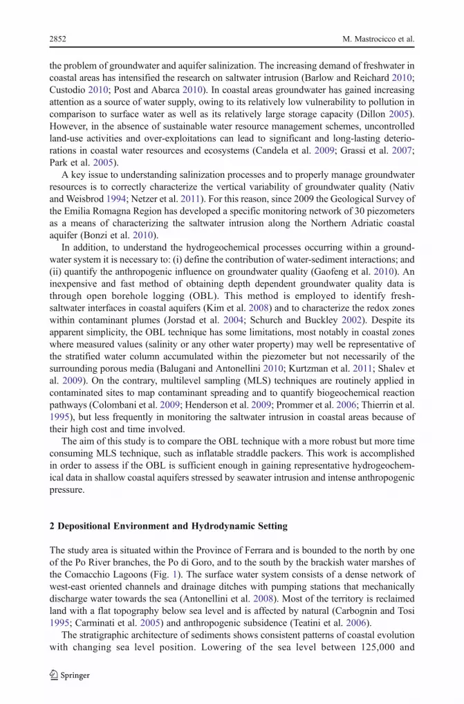
The study area is situated within the Province of Ferrara and is bounded to the north by oneof the Po River branches, the Po di Goro, and to the south by the brackish water marshes ofthe Comacchio Lagoons (Fig. 1). The surface water system consists of a dense network ofwest-east oriented channels and drainage ditches with pumping stations that mechanicallydischarge water towards the sea (Antonellini et al. 2008). Most of the territory is reclaimedland with a flat topography below sea level and is affected by natural (Carbognin and Tosi1995; Carminati et al. 2005) and anthropogenic subsidence (Teatini et al. 2006).

The stratigraphic architecture of sediments shows consistent patterns of coastal evolutionwith changing sea level position. Lowering of the sea level between 125,000 and

2852 M. Mastrocicco et al.

70,000 years ago resulted in extensive and repeated basinward shifts of facies, whichcan be observed across closely spaced unconformity surfaces associated with alluvialplain sedimentation (Amorosi et al. 2003). The general phase of sea level fall wasinterrupted by short transgressive phases, which led to the deposition of organic richdeposits (lagoons and swamps). The Holocene interglacial deposits were characterizedby a retrogradational stacking pattern of coastal plain and littoral facies, whichreflected landward migration of a barrier–lagoon–estuary system. The subsequenthighstand deposition was characterized by extensive progradation of wave influenceddeltas and strand plains (Amorosi et al. 2004).

During the last glacial lowstand, the modern coastal region was the site of middlealluvial plain sedimentation. In the contemporary coastal zone, transgressive accumu-lation started between 10,000 and 9,000 years ago. Back-stepping fluvial and brackishmarsh deposits were followed by delta-estuarine sand bodies, influenced by the lastimportant eustatic rise pulses. Early highstand saw the growth of large sand spits andbarrier islands, progressively turning the previous bays into confined lagoons (Stefaniand Vincenzi 2005).

This complex stratigraphic evolution led to a complex geometry of the aquifer. From eastto west, the majority of the sedimentary units consist of a wedge of permeable sandsediments deposited in shallow marine water, littoral sands formed in the foreshore and inthe adjacent beach, and sand dune systems (Antonellini et al. 2008). In the westernmost areafine continental alluvial deposits (mostly silt and clay) overlay the littoral sands (Amorosi etal. 2002; Bondesan et al. 1995).

The coastal aquifer is located mainly within the littoral sands and in the shallow marinewedge deposits. The thickness of the aquifer varies from 16 m to 22 m moving from theeastern to the western part of the study area (Fig. 2).

Fig. 1 Location of the study area with the piezometric contour map, canals network and borehole locations;in yellow the selected piezometers along a flow line (AB)

Data Aquisition is Saltwater Intrusion Monitoring 2853

3 Materials and Methods

3.1 Piezometer Installation

The four selected boreholes along transect AB (Fig. 2) are part of the regional monitoringnetwork of the costal aquifer, which, since 2009, have been equipped with piezometersinstalled by the Geological Survey of the Emilia-Romagna Region (Italy).

All wells (5 cm inner diameter) were screened from 1 m below ground level (b.g.l.) to amaximum of 22 m b.g.l. to fully penetrate the aquifer. The screens were not surrounded by asiliceous gravel pack to prevent cross contamination between sampling points, while ageotextile sock was used to minimize the piezometer clogging. The piezometers were sealedwith a mixture of cement and bentonite at the top to prevent surface-water infiltration. In twoboreholes, P33 and P34, core samples were collected every meter or when a change insediments was recognized. Samples were stored in a cool box at 4 °C and immediatelytransported to the laboratory for sediment analysis.

3.2 Stratigraphycal and Sedimentological Analysis

Particle size curves were obtained using a sedimentation balance for the coarse fraction andan X-ray diffraction sedigraph 5100 Micromeritics for the finer fraction; the two regions ofthe particle size curve were connected using the computer code SEDIMCOL (Brambati et al.1973). To describe grain size distribution analysis, the median of the average grain radius(expressed inφ), the 10th and 60th percentile of the cumulative curve (d10 and d60 expressedin φ) and the sorting were calculated. The organic matter content of the sediments wasmeasured by dry combustion (Tiessen and Moir 1993).

The hydraulic conductivity (k) of piezometers P33 and P34 was measured in thefield every 1 m by using an 800 L straddle packers system (Solinst, Canada) withsampling window of 0.2 m connected to a submersible centrifuge pump able todeliver 20 l/min. The head loss was measured by a levelogger LTC (Solinst, Canada)placed in between the two packers. The levelogger accuracy is ±0.01 m with amaximum pressure range of 10 m; below this depth the measurements are not reliable.Thus k values could not be accurately measured towards the bottom of the aquifer

Fig. 2 Transect AB (refer to Fig. 1 for the location). Topography (DEM data), water table (monitoring data ofNovember 2010), sandy aquifer thickness (dotted region) and stratigraphy (core logs data) are shown


and were limited to 10 m of saturated zone. k values (m/s) were derived from theequation (Bureau of Reclamation 2001):

k ¼ Q

CsrΔhð1Þ

where Cs (-) is the conductivity coefficient for semi-spherical flow in saturatedmaterials through partially penetrating cylindrical test wells and for these conditionis equal to 28, r (m) is the radius of the test well, Δh (-) is the head hydraulicgradient between static head and steady state head under pumping condition.

The water content was measured in saturated conditions gravimetrically after heating for24 h at 105 °C (Danielson and Sutherland 1986). Laboratory porosity measurements (n) oncore samples are often affected by errors, as many sampling methods alter the structure,packing and compaction of the sediment sample (Vienken and Dietrich 2011). Henceporosity values were also computed using the following empirical equation (Vukovic andSoro 1992):

nv ¼ 0:225 1þ 0:83ηð Þ ð2Þwhere η stand for uniformity coefficient, defined as d60[φ]/d10[φ].

The effective porosity (ne) was estimated with the formula (Worthington 1998):

ne ¼ n� CBW ð3Þwhere CBW is the clay-bounded water, which comprises electrochemically bound waterfrom clay surfaces and interlayers. The CWB varies in volume according to the clay-type,and the salinity of the formation water and can be estimated from (Hill et al. 1979):

CBW ¼ n� 0:6425�ffiffiffi

Sp

þ 0:22� �

� CEC ð4Þ

where S is the salinity (g/l) and CEC is the Cation Exchange Capacity (meq/ml of pore space).Finally, the pore water velocity along each piezometer was calculated following Darcy’s

law in the form of freshwater heads:

v ¼ kf � i!

neð5Þ

where v is the average pore water velocity (m/y), i!

is the freshwater hydraulic headgradient (-), ne is the effective porosity (-) and kf is the fresh water hydraulic conductivity (m/y).By assuming that salinity variations have a negligible effect on the groundwater kinematicviscosity, viscosity kf values can be considered similar to field-measured values of hydraulicconductivity (Post et al. 2007). In order to compute velocity values (v and vv in Tables 3 and 4),k values were obtained by Eq. 1 while effective porosity values (ne and nev) were calculated foreach core sample by Eq. 3 using both the measured total porosity (n) and the calculated total

porosity by Vukovic and Soro (1992) (nv). For the shallow coastal aquifer, a regional i!

influenced by the dewatering stations equal to 0.4‰ was applied.

3.3 Open Borehole Profiles and Multi-Level Sampling

In order to obtain the OBL profiles, a Hydrolab MS-5 (OTT, Germany) water quality probewas lowered into four boreholes to simultaneously record temperature, electrical conductiv-ity (EC), dissolved oxygen (O2), redox potential (Eh), pH and salinity. The Hydrolab MS-5


water quality probe consists of six sensors and a data transmitter mounted inside a 4.4 cmdiameter housing, with a 30 m long underwater cable and an YSI interface (YSI, California)at the ground surface. The Eh was corrected to the standard H+ electrode potential. Loggingwas carried out by lowering manually the multi-parameter probe into four piezometers P3,P8, P33, and P34 (Fig. 1). After a 5 min wait, the six parameters were simultaneouslyacquired every 1 m depth. The hydrochemical log measurements were made under naturalconditions, without purging the piezometers before the tests.

To acquire the MLS profiles, groundwater samples were collected every 1 m from thefour piezometers, by using an 800 L straddle packers system (Solinst, Canada). The sampleswere collected via a low-flow technique using an inertial pump, after measuring thegroundwater static level and purging of about 5 L. For each sample hydrochemical param-eters were acquired in situ by using a Hydrolab flow cell connected to the Hydrolab MS-5probe. Groundwater samples were then collected, filtered through 0.22 μm Dionex poly-propylene filters, stored in a cool box at 4 °C and immediately transported to the laboratoryfor chloride analysis. Chloride was analyzed using an isocratic dual pump ion chromatog-raphy ICS-1000 Dionex, equipped with an AS9-HC 4×250 mm high capacity column andan ASRS-ULTRA 4 mm self-suppressor for anions. An AS-40 Dionex auto-sampler wasemployed for the analyses, Quality Control (QC) samples were run every 10 samples and thestandard deviation for all QC samples run was greater than 4 %.

To compare data obtained by OBL and MLS techniques, the absolute residuals (theabsolute value observed using MLS minus the absolute value observed using OBL at thesame depth) and the linear regression coefficient (R2) with respect to the line YOBL 0 XMSL

was calculated for each parameter analyzed.

3.4 Continuous Monitoring of Piezometric Heads and Sea Level

In order to define groundwater temporal variations due to tidal fluctuations, a STS dataloggerDL/N Series 70 was placed in piezometer P8, located close to the coastline (≈1,400 m inland).The datalogger was set up for continuous barometric compensated level measurement andelectrical conductivity (one record per hour). The probe was placed in the saturated zone at4.5 m b.g.l. to capture groundwater fluctuations. The online data from Ravenna mareographerof ISPRAwere used (www.retemareografica.it) to compare groundwater fluctuations with tidalvariations. Sea level data from Ravenna mareographer have an average lag phase of about15 min with respect to the mareographer of Porto Garibaldi (http://www.provincia.fe.it/sito?nav0293&doc0E93B184E4E0ACBFCC125766900371819), positioned in proximity ofthe piezometer P8.

4 Results and Discussion

4.1 Hydrostratigraphycal Characterization

Tables 1 and 2 report the grain size distribution analysis performed on the samples ofpiezometers P33 and P34, respectively. The core sample analysis reveals a certain heterogeneityof the core logs, with very poorly sorted silty clay and peat lenses overlaying a highly permeablewell sorted sandy layer typical of high energy depositional environments, such as coastalenvironment (dunes and beaches), intercalated with poorly sorted sandy silt lenses. The sandyand sandy silt layers constituting the aquifer, are underlined throughout by an aquitard, inagreement with previous studies (Amorosi et al. 2003). Porosity values (Tables 1 and 2) range


http://www.retemareografica.it

http://www.provincia.fe.it/sito?nav=293&doc=E93B184E4E0ACBFCC125766900371819




between 18 % and 76 %, with high values due to the presence of peat layers exhibiting a highorganic matter content (OM%).

Tables 3 and 4 summarize the parameters measured (k) and derived from empiricalformulas (ne) used to calculate the mean groundwater flow velocities in piezometersP33 and P34 respectively. The estimated Peclet number (Pe), defined as (Bear 1972):

Pe ¼ v d=Df ð6Þ

where d is the average diameter of the grains constituting the aquifer (m), Df is thediffusion coefficient in pure water (m2/s) and v is the pore water flow velocity (m/s),is always below 1 and therefore the flow is dominated by diffusion-driven processes,or at least the role of diffusion is comparable to that of mechanical dispersion(Appelo and Postma 2005).

The estimated flow velocities show that seawater intrusion is proceeding inland at a veryslow rate due to the effects of the dewatering stations draining the recently reclaimed area ofthe Ferrara Province (Fig. 1). This confirms that the salinity present in the coastal shallowaquifer is mostly due to interactions between water and sediments deposited during the lasttransgressive period that was characterized by landward migration of a barrier–lagoon–estuary system.

Table 1 Core sample analyses of P33 borehole

i.d. Elevation O. M. Sand Silt Clay Median d10 d60 Sorting

m a.s.l % % % % φ φ φ φ

C01 −4.93 2.12 22.28 56.36 21.36 5.90 9.25 5.00 2.28

C02 −5.70 3.06 2.48 67.47 30.05 6.74 10.13 5.63 2.02

C03 −6.08 6.15 0.39 46.70 52.91 8.55 11.88 7.63 2.26

C04 −6.35 17.17 0.31 16.68 83.01 9.49 10.75 9.50 1.56

C05 −6.70 62.50 6.90 63.10 30.00 7.80 10.10 7.8 2.00

C06 −7.53 6.59 1.26 70.59 28.15 7.13 11.00 6.00 2.31

C07 −8.60 6.06 1.46 57.77 40.77 7.95 11.75 6.88 2.48

C08 −9.40 5.80 80.48 10.74 8.78 3.36 7.50 2.50 1.96

C09 −10.53 1.59 70.67 23.80 5.53 3.59 7.00 2.50 1.88

C10 −12.45 0.80 96.52 2.43 1.05 2.25 3.00 2.00 0.47

C11 −13.65 3.21 26.98 59.16 13.86 5.39 8.75 5.00 2.29

C12 −14.23 1.60 92.72 6.30 0.98 3.12 3.88 3.00 0.56

C13 −14.80 2.18 62.65 24.10 13.25 4.50 8.88 3.25 2.22

C14 −16.50 2.30 62.78 28.64 8.58 4.39 7.75 3.50 1.79

C15 −18.80 3.16 63.18 30.62 6.20 4.05 6.50 3.63 1.37

C16 −19.40 3.22 76.39 18.09 5.52 3.62 6.25 3.25 1.38

C17 −20.10 4.07 29.73 44.45 25.82 6.07 9.75 5.50 2.59

C18 −20.90 37.27 4.25 51.18 44.57 7.91 10.63 7.25 2.10

C19 −21.60 6.48 50.36 34.67 14.97 5.02 9.25 3.75 2.23

C20 −23.15 6.22 12.26 59.50 28.24 6.82 10.63 6.00 2.45

C21 −23.90 4.94 55.83 38.92 5.25 4.26 6.38 3.75 1.27

C22 −25.20 5.71 5.59 65.83 28.58 6.95 7.13 5.75 2.42

C23 −25.90 5.45 0.45 29.68 69.87 9.28 12.13 8.50 2.09


4.2 Tidal Forcing Effects on Groundwater Fluctuation

Figure 3 shows the relationship between tidal fluctuation and groundwater level in thepiezometer P8 from August 2009 to May 2010. From this plot it is clear that the tidalamplitude is approximately 0.4 m, the tidal range is 0.8 m and the average tidal level is0.18 ma.s.l., with the highest sea levels occurring during winter time due to storm events(Martinelli et al. 2010; National Marine Hydrographic Institute 1994). The piezometricheads recorded in the piezometer P8 meanwhile are quite stable in summer and earlyautumn, with a sudden 0.5 m decline in November 2009 and a steep rise in April 2010,following the irrigation/drainage canals regime. The general canals regime is regulated toprovide freshwater for agricultural purposes during the growing season and to drain precip-itation events during the wet season. Overall the maximum piezometric head variationduring the monitoring period was 0.89 m with a mean value of −1.66 ma.s.l.. The responseto precipitation events is good, with a groundwater level peak after every rainfall. During thewinter time the groundwater level rapidly decrease in absence of precipitations since theaquifer is not recharged by surface canals. In addition, in this season both sea level and

Table 2 Core sample analyses of P34 borehole

i.d. Elevation O. M. Sand Silt Clay Median d10 d60 Sorting

m a.s.l % % % % φ φ φ φ

C01 −3.80 7.81 1.44 42.85 55.71 8.56 11.75 7.75 2.33

C02 −4.60 7.68 7.38 50.52 42.10 7.66 11.13 6.63 2.62

C03 −6.50 1.65 92.69 5.85 1.46 2.80 3.63 2.75 0.58

C04 −7.50 1.09 96.64 2.73 0.63 2.18 2.88 2.00 0.46

C05 −8.50 1.34 94.56 4.00 1.44 2.09 3.00 2 0.69

C06 −12.50 5.04 64.68 29.63 5.69 4.03 6.63 3.50 1.40

C07 −14.10 10.61 55.58 34.08 10.34 4.61 8.13 3.63 1.99

C08 −15.50 4.87 71.51 23.55 4.94 3.99 6.38 3.50 1.26

C09 −16.50 6.67 13.76 48.86 37.38 6.75 10.25 5.25 2.47

Table 3 Values of measured total porosity (n), calculated total porosity by Vukovic and Soro (1992) (nv),respective effective porosity (ne, nev) and pore water velocity (v and vv), and measured hydraulic conductivity(k) in P33 borehole

i.d. Elevation n nv ne nev k v vvm a.s.l – – – – m/s m/y m/y

C05 −6.70 0.76 0.37 0.11 0.05 1.1e−4 12.8 26.5

C08 −9.40 0.33 0.29 0.27 0.24 2.1e−4 9.5 10.9

C09 −10.53 0.18 0.29 0.16 0.26 4.8e−5 3.8 2.3

C10 −12.45 0.27 0.35 0.26 0.34 1.2e−4 5.6 4.3

C11 −13.65 0.24 0.33 0.19 0.27 2.8e−5 1.9 1.3

C12 −14.23 0.25 0.37 0.24 0.35 2.6e−5 1.4 0.9

C13 −14.80 0.19 0.29 0.15 0.24 7.5e−6 0.6 0.4

C14 −16.50 0.20 0.31 0.17 0.26 4.3e−6 0.3 0.2

C15 −18.80 0.21 0.33 0.18 0.28 2.3e−6 0.2 0.1


groundwater table fluctuate accordingly with the “inverted barometric effect” (Balugani andAntonellini 2011). The low piezometric head variation during the hydrologic year shows thatthe unconfined aquifer is affected by the channel network and the fact that values are alwaysbelow the mean sea level confirm that the groundwater flow direction is always inland,favoring seawater intrusion. The right panel in Fig. 3 indicates the results of the analysisduring a shorter period of only 1 week, when the hydrometric level of the nearby canal wasstable and precipitation absent. In this period of time there is no evident correlation with thetidal fluctuation, in agreement with a recent study (Balugani and Antonellini 2011) whichdemonstrates that the tidal fluctuations are completely dampened within 200 m from thecoast line. During this period the recorded groundwater oscillations were most probably dueto variations of the canal’s hydrometric level. It can therefore be inferred that since P8 is the

Table 4 Values of measured total porosity (n), calculated total porosity by Vukovic and Soro (1992) (nv),respective effective porosity (ne, nev) and pore water velocity (v and vv), and measured hydraulic conductivity(k) in P34 borehole

i.d. Elevation n nv ne nev k v vvm a.s.l – – – – m/s m/y m/y

C03 −6.50 0.26 0.37 0.24 0.34 6.7e−5 3.6 2.5

C04 −7.50 0.25 0.35 0.24 0.34 6.2e−5 3.3 2.3

C05 −8.50 0.24 0.35 0.23 0.33 1.3e−5 0.7 0.5

C06 −12.50 0.25 0.32 0.21 0.27 1.9e−6 0.1 0.1

C08 −15.50 0.23 0.33 0.19 0.27 3.0e−6 0.2 0.1

Fig. 3 Plots of continuous piezometric head monitoring of piezometer P8 (black line) and sea level (red line).The left plot shows the entire monitoring period with also the precipitation events, while the right plot shows azoomed timeframe of 1 week when the tidal oscillation is more evident. Note that the y scales have differentranges and precipitations are scaled, offset and plotted in the sea level y axis


nearest piezometer to the coastline, the other piezometers along the monitored transect arenot affected by tidal fluctuations.

4.3 Hydrogeochemical Monitoring

Figure 4 shows the salinity profiles for the four piezometers along transect AB (Figs. 1 and2). Considering both OBL and MLS profiles, the aquifer overall displays fresh water(salinity <0.5 g/l) in the uppermost section of P3 and P8, from the top of the water tabledown to −9 and −6 ma.s.l. respectively, and a transition zone of brackish water (from 0.5 to30 g/l) with a thickness ranging from 1 to 4 m. As expected, the transition zone is thin due tothe minimal tidal fluctuations in this particular area of the Adriatic Sea, as explained above.Finally, saline (from 30 to 50 g/l) to hypersaline (>50 g/l) water is present in the remainingthickness of the aquifer (Barlow 2003).

Overall the absolute salinity residual for all the piezometers is 4.31 g/l and the R2 is 0.92,which is deemed an acceptable goodness of fit between the two techniques.

Since the two different acquisition techniques, i.e. the OBL and MLS methods, giveapproximately the same classification and distribution of the water types present in theaquifer, it follows that the OBL method can be successfully used for a preliminary determi-nation of the position of the saltwater wedge in aquifers with normal density stratification(freshwater near the water table and saline groundwater towards the bottom).

Nevertheless, analysing in more detail the OBL salinity profiles against the MLS profiles,some considerable differences are apparent. In P8 and P34 the OBL technique displays asomewhat constant concentration profile in the lower part of the aquifer where hypersalinewater is present. The MLS technique on the other hand, is able to distinguish in both

Fig. 4 Plots of salinity with MLS versus OBL data for each piezometer along transect AB; stratigraphy (corelogs data) from Fig. 2 is displayed on each plot to assist the interpretation


piezometers a considerable variability in the concentration profiles. In particular, the salinitydistribution in P8 slowly increases from saline (−8 ma.s.l.) to hypersaline water (−17 ma.s.l.),showing salinities always lower than the ones recorded at the same depths by OBL. In thehypersaline bottom part of the aquifer the deviation of the MLS profile from the OBL profile iseven more evident; in P34 theMLS profile shows a correlation between the salinity distributionand the stratigraphy, witnessing water-sediment interactions.

Accordingly in P33, the MLS profile demonstrates that the change in sediments reflects achange in salinity: at −20 ma.s.l. salinity increases up to 53 g/l in correspondence with apeaty layer.

It is also interesting to note that by plotting the Cl- versus salinity concentrationsfor all the analyzed groundwater samples (Fig. 5), a very close fit for salinity samplesbelow seawater composition is obtained, with a R2 value of 0.981. Using all theconcentration data meanwhile results in the fit degrading to a R2 value of 0.947. Thismeans that along this transect, salinity can be considered representative of a conser-vative species (like Cl-) only below seawater concentration, since above this concen-tration a large number of the observed values fall outside the 95 % confidenceinterval of the linear regression line (Fig. 5).

The misleading distribution of salinity values above seawater concentration recorded viathe OBL technique is thought to be due to both the mixing of water into the piezometersinduced by the density dependent flow and to the downward and upward movement of theprobe within the borehole casing during the monitoring procedure. These bias are obviouslyavoided using the MLS techniques.

As for the salinity values above seawater concentration, the OBL and MLS techniquespresent a discordant picture of the physico-chemical parameter profiles of the coastalshallow aquifer. Figure 6 describes pH profiles collected via OBL and MLS techniques.The profiles are not in good agreement, with an absolute residual for all piezometers of 0.37and an R2 value of 0.72. The pH measured by MLS is regularly higher than the onemeasured by the OBL technique, even if in both cases the ambient groundwater is charac-teristic of the basic environment.

Fig. 5 Plot of MLS salinity versus MLS Cl- concentration for all groundwater samples (open circles). Solidline indicates the linear regression line with 95 % confidence intervals (shaded area) and dashed line showsthe limit of seawater salinity


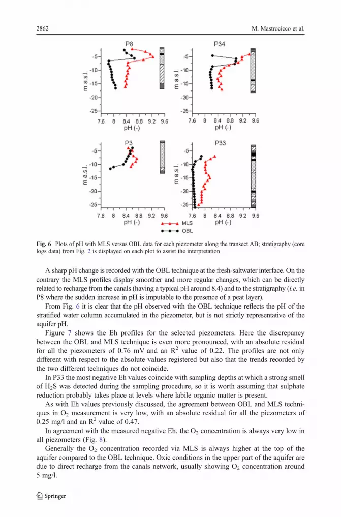
A sharp pH change is recorded with the OBL technique at the fresh-saltwater interface. On thecontrary the MLS profiles display smoother and more regular changes, which can be directlyrelated to recharge from the canals (having a typical pH around 8.4) and to the stratigraphy (i.e. inP8 where the sudden increase in pH is imputable to the presence of a peat layer).

From Fig. 6 it is clear that the pH observed with the OBL technique reflects the pH of thestratified water column accumulated in the piezometer, but is not strictly representative of theaquifer pH.

Figure 7 shows the Eh profiles for the selected piezometers. Here the discrepancybetween the OBL and MLS technique is even more pronounced, with an absolute residualfor all the piezometers of 0.76 mV and an R2 value of 0.22. The profiles are not onlydifferent with respect to the absolute values registered but also that the trends recorded bythe two different techniques do not coincide.

In P33 the most negative Eh values coincide with sampling depths at which a strong smellof H2S was detected during the sampling procedure, so it is worth assuming that sulphatereduction probably takes place at levels where labile organic matter is present.

As with Eh values previously discussed, the agreement between OBL and MLS techni-ques in O2 measurement is very low, with an absolute residual for all the piezometers of0.25 mg/l and an R2 value of 0.47.

In agreement with the measured negative Eh, the O2 concentration is always very low inall piezometers (Fig. 8).

Generally the O2 concentration recorded via MLS is always higher at the top of theaquifer compared to the OBL technique. Oxic conditions in the upper part of the aquifer aredue to direct recharge from the canals network, usually showing O2 concentration around5 mg/l.

Fig. 6 Plots of pH with MLS versus OBL data for each piezometer along the transect AB; stratigraphy (corelogs data) from Fig. 2 is displayed on each plot to assist the interpretation


Fig. 7 Plots of Eh with MLS versus OBL data for each piezometer along the transect AB; stratigraphy (corelogs data) from Fig. 2 is displayed on each plot to assist the interpretation

Fig. 8 Plots of O2 with MLS versus OBL data, for each piezometer along the transect AB; stratigraphy (corelogs data) from Fig. 2 is displayed on each plot to assist the interpretation


O2 concentration recorded via MLS decreases more rapidly with depth with respect toOBL, reaching anoxic condition within 1 to 3 m below the water table. Anoxic valuesmeanwhile are recorded between 4 to 7 m below the water table with the OBL technique.

The reactive sensitive physico-chemical parameter profiles (Figs. 6, 7 and 8) recorded viaOBL and MLS techniques give a conflicting overview of the coastal shallow aquifer, as forthe salinity values above seawater concentration (Figs. 4 and 5). This means that along thistransect, even if the two different acquisition techniques give approximately the sameclassification and distribution of the water types present in the aquifer, the OBL methodcannot be employed to characterize in detail the effects due to interactions between surfaceand ground waters. The OBL method is also shown to be inappropriate in defining the trendin the redox processes occurring within the aquifer, especially in correspondence withsediments bearing a high content of labile organic matter.

5 Conclusions

This study compares the open-borehole logging (OBL) technique with the more robust butmore expensive and time consuming multilevel sampling (MLS) technique. The work showsthat, excluding the distribution of saline to hypersaline water types in the bottom part of theaquifer, no significant differences are observed between salinity data recorded by means ofthe two techniques along the selected transect. It follows that, when the density stratificationis from denser groundwater at the bottom to less dense groundwater towards the water table,the OBL method can be successfully used for a preliminary determination of the position ofthe saltwater wedge and for a general classification and distribution of the water typespresent in the aquifer.

However, since hydrochemical data (pH, Eh, and O2) collected with the OBL techniquedo not agree with data acquired by the MLS technique, a more detailed study on the reactivegeochemical processes involving micro and meso-scale structures, like peat layers, can beundertaken only through MLS techniques. Indeed, this study demonstrates that the aboveeven holds when a high level of accuracy in depicting salinity distribution is required inorder to infer recharge from surface water bodies. It must be emphasized that in this studythe tidal forcing was negligible in most of the investigated piezometers, but tidal effects ongroundwater flow should generally be taken into account when monitoring seawater intru-sion (especially near to the shoreline) and not immediately ignored.

Acknowledgments Raffaele Pignone, Luciana Bonzi and Lorenzo Calabrese from Geological Survey ofEmilia-Romagna Region are acknowledged for their technical and scientific support. Umberto Tessari andEnzo Salemi from Earth Sciences Department of the University of Ferrara are thanked for the grain sizeanalysis. The authors wish to thank Mitchell Dean Harley (University of Ferrara) for his kind contribution inimproving the English text.

References

Amorosi A, Centineo MC, Colalongo ML, Pasini G, Sarti G, Vaiani SC (2003) Facies architecture and latestPleistocene– Holocene depositional history of the Po Delta (Comacchio area), Italy. J Geol 111:39–56

Amorosi A, Centineo MC, Dinelli E, Lucchini F, Tateo F (2002) Geochemical and mineralogicalvariations as indicators of provenance changes in Late Quaternary deposits of SE Po Plain. SedGeol 151:273–292


Amorosi A, Colalongo ML, Fiorini F, Fusco F, Pasini G, Vaiani SC, Sarti G (2004) Palaeogeographic andpalaeoclimatic evolution of the Po Plain from 150-ky core records. Glob Planet Chang 40:55–78

Antonellini M, Mollema P, Giambastiani BMS, Bishop K, Caruso L, Minchio A, Pellegrini L, Sabia M, UlazziE, Gabbianelli G (2008) Salt water intrusion in the coastal aquifer of the southern Po Plain, Italy.Hydrogeol J 16(8):1541–1556

Appelo CAJ, Postma D (2005) Geochemistry, groundwater and pollution, 2nd edn. Balkema, RotterdamBalugani E, Antonellini M (2010) Measuring salinity within shallow piezometers: comparison of two field

methods. J Water Resour Prot 2:251–258Balugani E, Antonellini M (2011) Barometric pressure influence on water table fluctuations in coastal aquifers

of partially enclosed seas: an example from the Adriatic coast, Italy. J Hydrol 400:176–186Barlow PM (2003) Ground water in fresh water-salt water environments of the Atlantic Coast. U.S.

Geological Survey circular; 1262Barlow PM, Reichard EG (2010) Saltwater intrusion in coastal regions of North America. Hydrogeol J

18:247–260Bear J (1972) Dinamics of fluids in porous media. Elsevier, AmsterdamBondesan M, Favero V, Vignals MJ (1995) New evidence on the evolution of the Po-delta coastal plain during

the Holocene. Quat Int 29(30):105–110Bonzi L, Calabrese L, Severi P, Vincenzi V (2010) L’acquifero freatico costiero della regione Emilia-

Romagna: modello geologico e stato di salinizzazione. Il Geologo dell’Emilia-Romagna—BollettinoUfficiale d’Informazione dell’Ordine dei Geologi Regione Emilia-Romagna, anno 10/2010 n. 39

Brambati A, Candian C, Bisiacchi G (1973) Fortran IV program for settling tube size analysis using CDC6200 computer. Istituto di Geologia e Paleontologia, Università di Trieste

Bureau of Reclamation (2001) Water testing for permeability. In: Engineering geology field manual, vol 2,chap 17. US Dept of the Interior, Washington, pp

Candela L, von Igel W, Elorza FJ, Aronica G (2009) Impact assessment of combined climate and managementscenarios on groundwater resources and associated wetland (Majorca, Spain). J Hydrol 376(3–4):510–527

Carbognin L, Tosi L (1995) Analysis of actual land subsidence in Venice and its hinterland (Italy). In: Landsubsidence. Balkema, Rotterdam, the Netherlands, pp 129–137

Carminati E, Dogliosi C, Scrocca D (2005) Magnitude and causes of natural subsidence of Venice. In: FletcherC, Spencer T (eds) Flooding and environmental challenges for Venice and its lagoon. CambridgeUniversity Press, Cambridge, pp 21–28

Colombani N, Mastrocicco M, Gargini A, Davis GB, Prommer H (2009) Modelling the fate of styrene in amixed petroleum hydrocarbon plume. J Cont Hydrol 105(1–2):38–55

Custodio E (2010) Coastal aquifers in Europe: an overview. Hydrogeol J 18:269–280Danielson RE, Sutherland PL (1986) In: Klute A (ed) Methods of soil analysis, part I. Physical and

mineralogical methods, 2nd edn. Agronomy monograph, 9: pp 443–461Dillon P (2005) Future management of aquifer recharge. Hydrogeol J 13(1):313–316Gaofeng Z, Yonghong S, Chunlin H, Qi F, Zhiguang L (2010) Hydrogeochemical processes in the ground-

water environment of Heihe River Basin, northwest China. Environ Earth Sci 60:139–153Grassi S, Cortecci G, Squarci P (2007) Groundwater resource degradation in coastal plains: the example of the

Cecina area (Tuscany – Central Italy). Appl Geochem 22:2273–2289Henderson TH, Mayer KU, Parker BL, Al TA (2009) Three-dimensional density-dependent flow and

multicomponent reactive transport modeling of chlorinated solvent oxidation by potassium permanga-nate. J Cont Hydrol 106:195–211

Hill HJ, Shirley OJ, Klein GE (1979) Bound water in shaly sands—its relation to Qv and other formation properties.The log analyst, volume XX(3), Society of professional well log analysts, May–June, 1979, pp 3–19

Jorstad LB, Jankowski J, Acworth RI (2004) Analysis of the distribution of inorganic constituents in a landfillleachate-contaminated aquifer: Astrolabe Park, Sydney, Australia. Environ Geol 46(2):263–272

Kim K-U, Chon C-M, Park K-H, Park Y-S, Woo NC (2008) Multi-depth monitoring of electrical conductivityand temperature of groundwater at a multilayered coastal aquifer: Jeju Island, Korea. Hydrol Processes 22(18):3724–3733

Kurtzman D, Netzer L, Weisbrod N, Graber E, Ronen D (2011) Steady-state homogeneous approximations ofvertical velocity from EC profiles. Ground Water 49(2):275–279

Lenahan MJ, Bristow K (2010) Understanding sub-surface solute distributions and salinization mechanisms ina tropical coastal floodplain groundwater system. J Hydrol 390:131–142

Martinelli L, Zanuttigh B, Corbau C (2010) Assessment of coastal flooding hazard along the Emilia Romagnalittoral, IT. Coast Eng 57:1042–1058

National Marine Hydrographic Institute (1994) Istituto Idrografico della Marina, 1994. Tavole diMarea (Mediterraneo – Mar Rosso) e delle correnti di Marea (Venezia – Stretto di Messina),Genova


Nativ R, Weisbrod N (1994) Management of a multilayered coastal aquifer—an Israeli case study. WaterResour Manag 8:297–311

Netzer L, Weisbrod N, Kurtzman D, Nasser A, Graber ER, Ronen D (2011) Observations on verticalvariability in groundwater quality: implications for aquifer management. Water Resour Manag25:1315–1324

Park SC, Yun ST, Chae GT, Yoo IS, Shin KS, Heo CH et al (2005) Regional hydrochemical study onsalinization of coastal aquifers, western coastal area of South Korea. J Hydrol 313:182–194

Post V, Abarca E (2010) Preface: saltwater and freshwater interactions in coastal aquifers. Hydrogeol J 18:1–4Post V, Kooi H, Simmons C (2007) Using hydraulic head measurements in variable-density ground water flow

analyses. Ground Water 45(6):664–671Prommer H, Tuxen N, Bjerg PL (2006) Fringe-controlled natural attenuation of phenoxy acids in a landfill

plume: integration of field-scale processes by reactive transport modelling. Environ Sci Technol 40(15):4732–4738

Schurch M, Buckley D (2002) Integrating geophysical and hydro-chemical borehole-log measurements tocharacterize the Chalk aquifer, Berkshire, United Kingdom. Hydrogeol J 10(6):610–627

Shalev E, Lazar A, Wollman S, Kington S, Yechieli Y, Gvirtzman H (2009) Biased monitoring of fresh water-salt water mixing zone in coastal aquifers. Ground Water 47(1):49–56

Stefani M, Vincenzi S (2005) The interplay of eustasy, climate and human activity in the late Quaternarydepositional evolution and sedimentary architecture of the Po Delta system. Mar Geol 222–223:19–48

Teatini P, Ferronato M, Gambolati G, Gonella M (2006) Groundwater pumping and land subsidence in theEmilia-Romagna coastland, Italy: modeling the past occurrence and the future trend. Water Resour Res42:1–19

Thierrin J, Davis GB, Barber C (1995) A groundwater tracer test with deuterated compounds for monitoring insitu biodegradation and retardation of aromatic compounds. Ground Water 33(3):469–475

Tiessen H, Moir JO (1993) Total and organic carbon. In: Carte ME (ed) Soil sampling and methods ofanalysis. Lewis Publishers, Ann Arbor, pp 187–211

Vienken T, Dietrich P (2011) Field evaluation of method for determining hydraulic conductivity from grainsize data. J Hydrol 400:58–71

Vukovic M, Soro A (1992) Determination of hydraulic conductivity of porous media from grain-sizecomposition, Water Resour Publ, Highlands Ranch, Colorado, pp 83

Worthington PF (1998) Conjunctive interpretation of core and log data through association of effective andtotal porosity models. In: Harvey PK, Lovell MA (eds), Core-log integration, geological society. London,Special Publications 136, pp 213–223


Documents

The Importance of Data Acquisition Techniques in Saltwater Intrusion Monitoring