Assessing impacts of climate change, sea level rise, and drainage canals on saltwater intrusion to coastal aquifer

HESSD9, 7969–8026, 2012

Assessing impactsof climate change,sea level rise, anddrainage canals

P. Rasmussen et al.

Title Page

Abstract Introduction

Conclusions References

Tables Figures

J I

J I

Back Close

Full Screen / Esc

Printer-friendly Version

Interactive Discussion

Discussion

Paper

|D

iscussionP

aper|

Discussion

Paper

|D

iscussionP

aper|

Hydrol. Earth Syst. Sci. Discuss., 9, 7969–8026, 2012www.hydrol-earth-syst-sci-discuss.net/9/7969/2012/doi:10.5194/hessd-9-7969-2012© Author(s) 2012. CC Attribution 3.0 License.

Hydrology andEarth System

SciencesDiscussions

This discussion paper is/has been under review for the journal Hydrology and Earth SystemSciences (HESS). Please refer to the corresponding final paper in HESS if available.

Assessing impacts of climate change, sealevel rise, and drainage canals onsaltwater intrusion to coastal aquiferP. Rasmussen1, T. O. Sonnenborg2, G. Goncear1, and K. Hinsby1

1Geological Survey of Denmark and Greenland, GEUS, Copenhagen, Denmark2Danish Nature Agency, Roskilde, Denmark

Received: 4 June 2012 – Accepted: 5 June 2012 – Published: 2 July 2012

Correspondence to: K. Hinsby ([email protected])

Published by Copernicus Publications on behalf of the European Geosciences Union.

7969

http://www.hydrol-earth-syst-sci-discuss.net

http://www.hydrol-earth-syst-sci-discuss.net/9/7969/2012/hessd-9-7969-2012-print.pdf

http://www.hydrol-earth-syst-sci-discuss.net/9/7969/2012/hessd-9-7969-2012-discussion.html

http://creativecommons.org/licenses/by/3.0/

HESSD9, 7969–8026, 2012


P. Rasmussen et al.

Title Page



Tables Figures

J I

J I

Back Close

Full Screen / Esc



Discussion

Paper

|D

iscussionP

aper|

Discussion

Paper

|D

iscussionP

aper|

Abstract

Groundwater abstraction from coastal aquifers is vulnerable to climate change and sealevel rise because both may potentially impact saltwater intrusion and hence groundwa-ter quality depending on the hydrogeological setting. In the present study the impacts ofsea level rise and changes in groundwater recharge are quantified for an island located5

in the Western Baltic Sea. Agricultural land dominates the western and central parts ofthe island, which geologically are developed as push moraine hills and a former lagoon(later wetland area) behind barrier islands to the east. The low-lying central area ofthe island was extensively drained and reclaimed during the second half of the 19thcentury. Summer cottages along the beach on the former barrier islands dominate the10

eastern part of the island. The main water abstraction is for holiday cottages during thesummer period (June–August). The water is abstracted from 11 wells drilled to a depthof around 20 m in the upper 5–10 m of a confined chalk aquifer. Increasing chlorideconcentrations have been observed in several abstraction wells and in some casesthe WHO drinking water standard has been exceeded. Using the modeling package15

MODFLOW/MT3D/SEAWAT the historical, present and future freshwater–sea waterdistribution is simulated. The model is calibrated against hydraulic head observationsand validated against geochemical and geophysical data from new investigation wells,including borehole logs, and from an airborne transient electromagnetic survey. Theimpact of climate changes on saltwater intrusion is found to be sensitive to the bound-20

ary conditions of the investigated system. For the flux-controlled aquifer to the west ofthe drained area only changes in groundwater recharge impacts the freshwater–seawater interface whereas sea level rise do not result in increasing sea water intrusion.However, on the barrier islands to the east of the reclaimed area below which the seais hydraulically connected to the drainage canal, and the boundary of the flow sys-25

tem therefore controlled, the projected changes in sea level, groundwater rechargeand stage of the drainage canal all have significant impacts on saltwater intrusion andhence the chloride concentrations found in the abstraction wells.

7970





HESSD9, 7969–8026, 2012


P. Rasmussen et al.

Title Page



Tables Figures

J I

J I

Back Close

Full Screen / Esc



Discussion

Paper

|D

iscussionP

aper|

Discussion

Paper

|D

iscussionP

aper|

1 Introduction

Climate change impacts especially sea level rise and changed precipitation patternswill challenge the current water supply management and groundwater abstraction fromwell fields close to the coast.

Previous studies of seawater intrusion (SWI) and salt water distribution in coastal5

aquifers have focused on mapping of salt water occurrence, fluid-density aspects ofnumerical flow modeling, effects of drainage in a polder context, effects of autonomoussalinization, tidal effects, and parameter estimation (Essink et al., 2001; Post, 2005;Carrera et al., 2010; de Louw et al., 2011). More recently several studies have fo-cused on using geophysical data and groundwater age data for corroboration of SWI10

models (Goes, 2009; Vandenbohede et al., 2011; Kirkegaaard, 2011), as SWI modelsmay be significantly improved by the use of efficient geophysical (e.g. airborne electro-magnetic, AEM) measurements (Comte and Banton, 2007; Comte et al., 2010; Carreraet al., 2010). Presently, focus is very much on climate change effects on seawater intru-sion and saltwater distribution in coastal aquifers (Werner and Simmons, 2009; Essink15

et al., 2010; Webb, 2011; Chang, 2011).In addition to sea level rise, most climate models predict an increase in winter pre-

cipitation for the Danish area. An increased winter precipitation will most likely increasegroundwater recharge (van Roosmalen et al., 2007), which is expected to counteractthe effect of sea level rise. Studies of the effects of sea level rise, changed recharge20

and drainage elevations on seawater intrusion to coastal groundwater aquifers aredescribed by Feseker (2007), Vandenbohede et al. (2008), Essink et al. (2010), andSulzbacher et al. (2012). Chang et al. (2011) investigated the impact of sea-level riseon an idealized coastal aquifer system and showed that for confined systems wherethe ambient recharge to the aquifer remains constant, sea-level rise has no long-term25

impact on the saltwater wedge. Groundwater level is found to increase in response tosea-level rise and potential intrusion effects are therefore mitigated. Werner and Sim-mons (2009) further show that the inland boundary conditions are crucial for the effect

7971





HESSD9, 7969–8026, 2012


P. Rasmussen et al.

Title Page



Tables Figures

J I

J I

Back Close

Full Screen / Esc



Discussion

Paper

|D

iscussionP

aper|

Discussion

Paper

|D

iscussionP

aper|

of sea-level rise on the evolution of the saltwater wedge of unconfined aquifers. Forconstant flux conditions similar to those used by Chang et al. (2011), where the dis-charge through the aquifer is assumed to be the same with and without sea-level rise,only small changes in the location of the wedge is found for typical aquifer character-istics. However, for head-controlled systems where the inland hydraulic head remain5

unchanged during sea-level changes, the saltwater wedge are predicted to migratehundreds of meters to several kilometers inland for a realistic sea-level rise. Study ar-eas where the water table is controlled by drainage systems are therefore expected tobe more vulnerable to future changes in sea level than natural systems.

The objectives of this paper are to investigate the following questions:10

(a) What is the effect of climate change, including sea level rise and changed ground-water recharge, on an aquifer in an area where the groundwater head is partly con-trolled by drainage canals? The importance and effect of drainage canals is analyzedthrough selected climate scenarios and canal stage scenarios. The effects on theaquifer as such and on the actual groundwater abstraction wells are analyzed. (b) What15

are the most important factors for seawater intrusion to a coastal aquifer; sea level rise,changes in groundwater recharge or water level in the drainage canals? (c) What arethe dynamics of increased seawater intrusion in combination with increased recharge?Increased recharge might counteract saltwater intrusion as an effect of sea level rise.Dynamics and time lags are analyzed in this real-world case study. (d) Will the water20

works have to move some of their wells in the area in the 21st century due to saliniza-tion?

Hydrochemical data, groundwater age data, airborne geophysics, and borehole log-ging are all used to corroborate the results from the established SWI model.

7972





HESSD9, 7969–8026, 2012


P. Rasmussen et al.

Title Page



Tables Figures

J I

J I

Back Close

Full Screen / Esc



Discussion

Paper

|D

iscussionP

aper|

Discussion

Paper

|D

iscussionP

aper|

2 Materials and methods

2.1 The study area

The study area is located in the southern part of the island of Falster in southeasternpart of Denmark (Fig. 1). To the east the area is confined by the Baltic Sea and to thewest by the strait of Guldborgsund. The top elevation varies from 19 m above mean5

sea level (m a.s.l.) to −7 m a.s.l. to the east of the model area. The landscape is mainlydeveloped from north-south trending low push moraine hills of clayey tills along thecoast in the western part of the island, which were formed during the last glaciation byan east to west moving glacier. During the Holocene small barrier islands with eoliansand dunes, which constitute the eastern part of the island, and a lagoon developed10

in front of the glacial moraine hills. As the barrier islands grew it became possible toreclaim the low-lying wetland area between the push moraine and the barrier islandsin the central part of the study area (Fig. 2). In the early 18th century only a small straitto the south made a connection between the shallow lagoon, and the Baltic Sea. Inthe period 1860–1865 the strait was closed by a dike and the drainage of Bøtø Nor15

started. In 1871 a pumping station was established and after a major storm in 1872a 17 km new long dike was build and the area was drained and converted into farmland. The pumping station is pumping water from the drainage system to the Marrebækcreek discharging to the strait of Guldborgsund at the western coastline (Fig. 2). Thereclaimed low-lying area is dominated by marine post-glacial sands deposited on top20

of a clayey ground moraine.The land use in the study area is dominated by agriculture and settlements of sum-

mer cottages although a few small permanent villages have developed on top of thepush moraine hills in the western part of the area. The first summer cottages werebuilt in the Marielyst area in 1908 on the barrier islands along the eastern coastline.25

Around 1940 more than 500 houses existed in the area. In the 1960s and 1970s theconstruction of houses exploded and today there are more than 5000 summer cot-tages. Although most of these are built on the original barrier islands in the eastern

7973





HESSD9, 7969–8026, 2012


P. Rasmussen et al.

Title Page



Tables Figures

J I

J I

Back Close

Full Screen / Esc



Discussion

Paper

|D

iscussionP

aper|

Discussion

Paper

|D

iscussionP

aper|

part of the investigated area, the most recent have spread into the reclaimed areasand some of these are therefore located at or below sea level. As estimated from theseasonal variation in abstraction, 10–15 % of the houses are now used as year-roundresidence. The freshwater supply for the village and the summer cottages is basedsolely on groundwater. In this study we focus on the evolution of the salt (chloride) con-5

tents of the 11 water abstraction wells of Marielyst Waterworks supplying the summercottages as the salinity of these are increasing (Fig. 3) and some already have beentaken out of production.

As described above part of the area has undergone significant changes during thelast centuries from a brackish lagoon connected to the Baltic Sea to a lake, and finally10

to drained and reclaimed land mainly used for agriculture. The salinization effects ofthese changes have been included in the study by modeling four consecutive hydro-graphical phases leading up to the present situation.

2.1.1 Geology and hydrogeology

The geology down to 30 m below ground surface are quite well described with geo-15

logical information from more than 70 boreholes in the area. However, only four wellsare deeper than 50 m and no well is deeper than 100 m meaning that information onthe deep geology is limited. Information on off-shore geology is scarce. A marine rawmaterials mapping indicates that from the shore line and 1 to 2 km to the east the bot-tom sediments consists of fine to medium grained sand, whereas further to the east20

the bottom sediments are clayey till (Kuijpers, 1991). The Quaternary sediments con-sist mainly of clayey tills with local sand lenses. The thicknesses of the Quaternarydeposits are up to 45 m in the center and southwest of the area, and down to 5–10 munder the post-glacial sands. The postglacial marine sands and the eolian dunes maybe up to 10 m thick. The pre-quaternary surface consists of several hundred meters of25

Maastrichtian chalk.The main aquifer for water supply in the area is the upper chalk. The Quaternary

glaciations have caused fracturing of the upper 20–30 m of the chalk where the chalk7974





HESSD9, 7969–8026, 2012


P. Rasmussen et al.

Title Page



Tables Figures

J I

J I

Back Close

Full Screen / Esc



Discussion

Paper

|D

iscussionP

aper|

Discussion

Paper

|D

iscussionP

aper|

is fully or partly refreshed due to fast advective groundwater flow through the fractures.Previous studies of chalk aquifers in Denmark have shown that the residual saltwater isflushed out in the upper 50–80 m of the chalk by infiltrating fresh water (Bonnesen et al.,2009). Below this zone a mixing zone with higher chloride concentrations is seen wherethe number of fractures and the effective hydraulic conductivity is gradually decreas-5

ing compared to the fully refreshed zone above. Below this depth matrix diffusion isthe dominating transport process for saltwater (Bonnesen et al., 2009). At depth below150–200 m the saltwater is of oceanic concentration with total dissolved solids concen-trations above 35 000 mgTDSl−1 and chloride concentrations above 19 000 mgl−1.

2.1.2 Hydrology10

The average annual precipitation in the area is approximately 700 mm. Based on re-sults from the national water resources model. The DK-Model (Henriksen et al., 2003,2008; Højberg et al., 2008), groundwater recharge has been estimated on daily basisfor the period 1990–2010. For the present study area the annual variation in the periodwas 79–437 mmyr−1. The surface water system is dominated by the artificial drainage15

canal system. A few minor creeks flow towards the drainage system or towards Guld-borgsund. The drainage system is lowering the groundwater table in the area wherethe ground surface is between +1 and −3 m a.s.l. The pumping station is aiming atkeeping a constant water level in the drainage canals. During a field campaign the wa-ter level in the drainage system were measured at several locations across the drained20

area and the stages were found to vary between −1 and −2.5 m a.s.l.The Marielyst waterworks supplies water to 5200 households mainly summer cot-

tages with drinking water. Due to the high percentage of summer cottages in thearea the groundwater supply varies considerably during the year with a maximum of2000 m3 day−1 in July to a minimum of 300 m3 day−1 in January. The waterworks has25

11 active abstraction wells which are located in three well fields (Figs. 2 and 5). Theoldest well field is located about 0.5 km from the coast, a second group of wells are ap-proximately 1 km from the coast (established 1975–1990), both well fields are located

7975





HESSD9, 7969–8026, 2012


P. Rasmussen et al.

Title Page



Tables Figures

J I

J I

Back Close

Full Screen / Esc



Discussion

Paper

|D

iscussionP

aper|

Discussion

Paper

|D

iscussionP

aper|

on one of the former barrier islands. The newest well field is located in the centralpart of the island 2.5 km from the coast lines, and established in 2005 in or very closeto the main groundwater recharge area in the push moraine hills. Individual pumpingrates or pumping schemes for each well were not available for this study. All 11 wa-ter abstraction wells of Marielyst waterworks are drilled to a depth of 10–15 m into the5

upper fractured chalk aquifer (Jupiter, 2011). Significant groundwater abstraction hastaken place since the 1960s. The annual groundwater production reached its maximumaround 470 000 m3 yr−1 in the beginning of the 1980s and has since then decreased tothe present level of around 250 000 m3 yr−1, mainly due to repair of leaky water pipes.

Additionally, groundwater abstraction takes place from two other minor waterworks10

and a few irrigation wells, which add up to approximately 150 000 m3 yr−1. The totalgroundwater abstraction in the model area is around 0.4×106 m3 yr−1. The pump-ing station is pumping 6.5×106 m3 yr−1 out of the area including approximately 0.7×106 m3 yr−1 of treated sewage water, which has been discharged to the canal froma wastewater treatment plant.15

The tidal amplitude in the area is relatively small, less than 0.2 m, therefore tidaleffects have been ignored in this study.

2.1.3 Groundwater chemistry in water supply wells

As described in the previous section the water supply wells of Marielyst Waterworkshas 11 wells grouped in three well fields at different distances to the sea (well field20

1–3; Fig. 5). Only 10 wells are currently active, however, one of the wells in well field1 is taken out of production. General groundwater chemistry of major ions were anal-ysed approximately once a year in all water supply wells since 1985 (since 2006 inthe newest well field). During this period all wells show steadily increasing chlorideconcentrations (Fig. 3). Only one well (242.178) in well field 1 closest to the sea is25

still active although it has concentrations above the WHO/EU drinking water standardof 250 mgl−1. Another well (242.44B) located at the waterworks have chloride analy-ses back to 1970 (148 mgl−1) and until 2004 (293 mgl−1) where it was taken out of

7976





HESSD9, 7969–8026, 2012


P. Rasmussen et al.

Title Page



Tables Figures

J I

J I

Back Close

Full Screen / Esc



Discussion

Paper

|D

iscussionP

aper|

Discussion

Paper

|D

iscussionP

aper|

production due to elevated chloride concentrations above the drinking water standard.Well field 3 was established at approximately the same time to support increasing de-mands and ensure the supply for all consumers. In addition to the general geochemistryanalysis of major ions all wells were also analysed every 3–4 yr for contaminants suchas organic micro contaminants, pesticides and nitrate as described in the Danish mon-5

itoring programme. Generally, there are no traces of contaminants or human impactson the extracted groundwater indicating that the groundwater pumped for water supplyrecharged the chalk aquifer prior to 1950 (e.g. Hinsby et al., 2001).

3 Data collection and investigations conducted in the project

Groundwater samples were collected from selected water supply wells in collaboration10

between GEUS and the waterworks for the analysis of general hydrochemistry andgroundwater age estimation by the environmental tracers 3H/3He.

– General hydrochemistryMajor ion analyses were performed in the laboratory at GEUS by atom absorp-tion spectroscopy (Ca), ion chromatography (Na, K, Mg, Cl, Br, F, SO2−

4 ), FIA/Flow15

Injection Analysis (NH4+) and spectroscopy (PO3−4 ). Alkalinity was measured in

the field by Gran titration, while O2, pH and SEC (specific electrical conductiv-ity) were measured by standard WTW electrodes in the field. The total dissolvedsolids were calculated manually from the analysis of the major cations and anions,after checking of the ion balance for every sample.20

– 3H/3HeSamples for 3H, He isotopes and Ne analysis and groundwater dating were col-lected in two copper tubes (for noble gases) and a 1 l plastic bottle (for 3H) by sam-pling techniques provided by the “Helis-Helium Isotope Studies Bremen” (Univer-sity of Bremen), where the collected samples were analysed by mass spectrom-25

etry (Sueltenfuss et al., 2009). Tritium (3H) is determined by the helium-in-growth7977





HESSD9, 7969–8026, 2012


P. Rasmussen et al.

Title Page



Tables Figures

J I

J I

Back Close

Full Screen / Esc



Discussion

Paper

|D

iscussionP

aper|

Discussion

Paper

|D

iscussionP

aper|

method where the decay product of 3H (3He) is measured by mass spectrometrywith a detection limit of 0.01 TU (1 TU= 3H/2H ratio of 1×10−18).

3.1 Airborne geophysics and borehole logging

Borehole logging (Buckley et al., 2001) and airborne electromagnetics (AEM) by theSkyTEM method (Sørensen and Auken, 2004) have proven their value for the mapping5

of the fresh and saltwater distribution in the subsurface in Danish geological settings(Buckley et al., 2001; Kirkegaard et al., 2011; Jørgensen et al., 2012). We thereforeused these methods to provide valuable data on salinity variations in the subsurfacefor the model setup and for corroboration of the simulation results in the investigatedarea. The geophysical investigations were conducted as part of the present study10

mainly to supplement the existing knowledge of the lithological variations (distributionof aquitards and aquifers), groundwater flow in aquifers, and the subsurface distributionof saltwater.

– Borehole loggingBorehole wireline geophysics were conducted by GEUS in 14 wells, including15

three new wells drilled during the project, primarily to evaluate the fresh/salt waterboundaries (Fig. 2). The logging program was conducted using standard slimholelogging equipment (by Robertson Geologging LTD). The collected data are usedto evaluate geological stratification, saltwater distribution and groundwater flowinto wells (e.g. Buckley et al., 2001; Maurer et al., 2009), and to support and20

corroborate the interpretation of the regional airborne SkyTEM measurements(Jørgensen et al., 2012). The combined use of logging probes measuring naturalgamma radiation, formation conductivity (focused induction log), fluid conductivityand temperature and inflow to wells (propeller flow meter) were applied to e.g.identify whether low formation resistivities are due to saline porewaters or high25

clay contents in sediments (Sanchez et al., 2012) and to identify hydraulic activezones in the Chalk aquifer.

7978





HESSD9, 7969–8026, 2012


P. Rasmussen et al.

Title Page



Tables Figures

J I

J I

Back Close

Full Screen / Esc



Discussion

Paper

|D

iscussionP

aper|

Discussion

Paper

|D

iscussionP

aper|

– AEM (SkyTEM)An airborne (Helicopter) time domain electromagnetic survey (SkyTEM, Sørensenand Auken, 2004) was flown over areas covering most of well field 2 and 3.The SkyTEM system was developed for high – resolution surveys for espe-cially hydrological targets. In this particular SkyTEM survey an average helicopter5

speed of 13 ms−1 was chosen and the transmitter (314 m2 octagonal loop) setup with a low moment (10A×314m2 ×1turn = 3140Am2) and a high moment(100A×314m2 ×2turns = 62800Am2), enabling shallow and deep penetration,respectively, and allowing TEM measurements every 30 m with a depth of inves-tigation of up to 120–150 m (Auken et al., 2009a). Unfortunately, due to a large10

number of electrical cables, it is not possible to measure in the housing areasalong the eastern coastline and around well field 1. The survey provides resistiv-ity or electrical conductivity maps of the subsurface indicating e.g. the distributionof saltwater in aquifers (Auken et al., 2009b; Kirkegaard et al., 2011; Jørgensenet al., 2012). Approximately 50 km of SkyTEM were flown in the investigated area15

with a distance between fligthlines of 150–200 m. The data was processed and in-verted with Spatially Constrained Inversion algorithm (Viezzoli et al., 2008), usingthe Aarhus Workbench software (Auken et al., 2009b; Aarhus Geophysics, 2009).

3.2 Flow and transport model

The numerical modeling complex MODFLOW-2000/MT3DMS/SEAWAT was used for20

simulating the 3-D variable density groundwater flow and solute transport (Harbaughet al., 2000; Zheng and Wang, 1999; Zeng, 2010; Langevin et al., 2007). The userinterface Groundwater Vistas version 6 was used as the pre- and post-processing tool(Rumbaugh and Rumbaugh, 2011).

The groundwater abstraction, the groundwater recharge, and the drainage canals25

are simulated with the MODFLOW Well Package, the Recharge Package, and theDrainage Package. The Time-Variant Specified-Head (CDH) package is used to as-sign specified or constant head boundaries that can change within or between stress

7979





HESSD9, 7969–8026, 2012


P. Rasmussen et al.

Title Page



Tables Figures

J I

J I

Back Close

Full Screen / Esc



Discussion

Paper

|D

iscussionP

aper|

Discussion

Paper

|D

iscussionP

aper|

periods (Harbaugh et al., 2000). When using the CHD package for variably densitymodeling the reference head value assigned to the boundary cell is updated prior toeach transport timestep using the fluid density from the previous transport timestep(Langevin et al., 2007).

The Hydrogeologic-Unit Flow (HUF) Package was used for the MODFLOW-20005

program (Anderman, 2000). The HUF package is a flow-package that makes it pos-sible to define hydrogeological units that are independent from the numerical layers.Hydraulic properties are assigned to the hydrogeological units in the HUF packageand the HUF package calculates the effective hydraulic properties for the numericallayers. The advantage of using the HUF package in variable density modeling is the10

ability on the one hand to represent hydrological units of variable thickness and distri-bution and at the same time honor the recommendations of using horizontal numericallayers of uniform thickness for the density modeling (Langevin et al., 2007).

The Preconditioned Conjugate-Gradient (PCG2) Package is used to solve the flowequations.15

Due to the length of simulation time the finite difference solution scheme is used forsolving the advection term of the solute transport equation in the first three modelingphases despite the risk of numerical dispersion. For the three last model phases in-cluding the scenario simulations the TVD method is used. The TVD method introducesonly limited numerical dispersion. The Generalized Conjugate solver (GCG) with the20

SSOR pre-conditioner is used for solving the sink/source and dispersion terms.A sensitivity analyses is performed comparing the use of the Finite Difference solu-

tion scheme compared to the TVD solution scheme on the effect on salinity in ground-water abstraction wells.

For SEAWAT v4 the Variable-Density Flow (VDF) package is used. The density–25

concentration slope is defined in the VDF package.

7980





HESSD9, 7969–8026, 2012


P. Rasmussen et al.

Title Page



Tables Figures

J I

J I

Back Close

Full Screen / Esc



Discussion

Paper

|D

iscussionP

aper|

Discussion

Paper

|D

iscussionP

aper|

3.3 Scenarios

The central part of Falster has, as described above, undergone several significantchanges in the hydrological system during the last centuries. These changes may be di-vided into four phases, Fig. 4. Until mid-last millennium (phase 1) the lagoon was opento the Baltic Sea and the water was salt/brackish. Due to the sedimentation around5

the barrier islands the outlet between the lagoon and the Baltic Sea became narrowerand the water in the lagoon became fresher (phase 2). Around 1870 the connectionto the sea was closed and the reclamation and drainage of the area was initiated anda pumping station built (phase 3). Later a waterworks was established on one of thebarrier islands and groundwater abstraction was initiated (phase 4). This four-phase10

transition from saltwater lagoon to groundwater abstraction area forms the initial condi-tions for the climate scenarios (Table 1). An autonomous salinization might be ongoing,i.e. the aquifer system may not be in dynamic equilibrium with respect to salinizationafter these changes in the hydrological system.

The scenarios focus on two aspects of climate change: sea level rise and change in15

groundwater recharge. The basic climate scenario includes a sea level rise of 0.75 mand an increase in groundwater recharge of 15 % or 36 mm in the period from 2010to 2100 (phase 5). The increase in groundwater recharge is based on van Roos-malen (2007) who has estimated the expected change in groundwater recharge fora comparable area in Denmark based on output from regional climate models repre-20

senting IPCC scenarios A2 and B2. In phase 6 both recharge and sea level are keptconstant for additional 200 yr to capture the long-term effects of the imposed climatechanges (Fig. 4).

Eight climate change scenarios were simulated with different combinations of sealevel rise, groundwater recharge, and drainage canal stage (Table 2). Scenario 0 rep-25

resents a situation where no changes occur. Scenario 1 represents an estimate of themost likely future with an increase in recharge of 15 % and sea level rise of 0.75 m.In scenario 2–8 a sensitivity analysis of the most likely scenario is carried out, where

7981





HESSD9, 7969–8026, 2012


P. Rasmussen et al.

Title Page



Tables Figures

J I

J I

Back Close

Full Screen / Esc



Discussion

Paper

|D

iscussionP

aper|

Discussion

Paper

|D

iscussionP

aper|

realistic changes in sea level and recharge have been implemented. The drainagecanals play an important role in the modeled groundwater system. To evaluate the sen-sitivity of the drains two simulations (scenarios 7 and 8) are performed with changedstage, +30 cm and −30 cm.

4 Model setup, calibration and validation5

4.1 Hydro-stratigraphic model

The hydrogeological model is based on the hydro-stratigraphic layers defined in the DK-model (Højberg et al., 2008). The DK-model consists of eight alternating Quaternaryclayey till and sand layers below which the pre-quaternary sediments consisting ofchalk is defined. The surfaces and thicknesses of the model layers in the DK-Model10

have been estimated on the basis of the extensive Danish well record database Jupiterwith more than two wells per square kilometer (national average), geological maps andmodels, and regional geophysical surveys. The hydro-stratigraphic model layers areinterpreted in horizontal/lateral resolution of 100m×100m grid.

In the present study area three adjustments of the hydro-stratigraphic layers have15

been made. Based on the soil map and geological information from wells, a top layerof 5 m sand is implemented where the soil map shows sand. Clayey till is assignedelsewhere in the top layer. The upper five meters of the clayey till is assumed fracturedwith a higher hydraulic conductivity than deeper laying clayey till (Højberg et al., 2008).Based on studies of comparable Chalk formations in Denmark, Bonnesen et al. (2009)20

suggest that the upper 30–80 m of the Chalk is fully refreshed due to fracture systemsallowing freshwater to circulate and displace the original marine saltwater. The stratifi-cation of the upper part of the chalk aquifer may be conceptualized in three units: an up-per zone crushed by glacial activities with many fractures, high effective hydraulic con-ductivity and dominated by advective groundwater flow; an intermediate fractured and25

7982





HESSD9, 7969–8026, 2012


P. Rasmussen et al.

Title Page



Tables Figures

J I

J I

Back Close

Full Screen / Esc



Discussion

Paper

|D

iscussionP

aper|

Discussion

Paper

|D

iscussionP

aper|

partly refreshed mixing zone (Bonnesen, 2009; Klitten, 2006) with a medium hydraulicconductivity; and a deeper zone with low hydraulic conductivity dominated by diffusion.

In order to represent an upper zone where solute transport is dominated by advec-tion and a deeper zone where solute transport is dominated by diffusion, the chalkformation has been divided into eight hydro-stratigraphic layers with gradually decreas-5

ing hydraulic conductivity. The upper four layers have a thickness of 15 m while thelower four layers have a thickness of 30 m. The hydro-stratigraphic layers of the chalkformation follow the topography of the chalk, the pre-quaternary surface.

4.2 Model setup

The model area covers an area of 44 km2 where 12 km2 or 27 % of the area is sea10

(Fig. 5). Horizontally a grid size of 50 m by 50 m is used while in the vertical 32 numer-ical layers with thicknesses varying from 2 m to 12 m are specified, adding to a totalnumber of active cells of 560 640. The thickness of the numerical layers gradually in-creases with depth down to −200 m a.s.l. The top elevation follows the digital terrainmodel including the elevation of the sea floor. In order to ensure that the drainage canal15

is located in the top layer the bottom of the top layer is specified at 4 m below groundsurface. A minimum of 2 m layer thickness means that the model layer topography hasbeen modified in the sea area.

The boundary conditions of the model include constant head in the uppermost modellayer in the area representing the sea, drains in 848 cells, no-flow along the outer20

boundaries, as well as groundwater recharge and groundwater abstraction. A horizon-tal impermeable layer at −200 m depths defines the bottom of the numerical model.

The simulation of seawater intrusion has been divided into six phases (Fig. 4) usingfour separate but consecutive model setups and simulations with different boundaryconditions (Table 3) to represent the historical situation. The groundwater head and25

salinity distribution at the end of each model phase was used as initial heads and con-centrations for the consecutive model phase. In phase one the saltwater concentrationin the lagoon, Bøtø Nor, and the water table is assumed to be the same as the Baltic

7983





HESSD9, 7969–8026, 2012


P. Rasmussen et al.

Title Page



Tables Figures

J I

J I

Back Close

Full Screen / Esc



Discussion

Paper

|D

iscussionP

aper|

Discussion

Paper

|D

iscussionP

aper|

Sea, 10 500 mgTDSl−1 and 0 m a.s.l., respectively. To reach a steady state situation forthe saltwater-freshwater distribution of the modeled system a 3000 yr simulation periodwas performed. The lagoon area was delineated based on a map from 1780 (Fig. 2).The second model phase from 1600 to 1870 is characterized by fresh water in the la-goon and a water table 0.2 m above the Baltic Sea. In the third phase representing the5

period after 1870 where the reclamation and drainage on the old lagoon area startedthe constant head in the lagoon area is replaced by a system of drainage canals. Thefourth period starts in 1960 where substantial groundwater abstraction began. 11 ab-straction wells with constant abstraction rate are introduced in model.

The implementation and impact of the climate changes were modeled through addi-10

tional two model phases (Fig. 4). The effects of sea level rise and changed groundwaterrecharge are gradually implemented in the fifth model phase from 2010 to 2100. At thebeginning of each 10-yr period one tenth of the change is applied to the model, whichmeans that the first change is implemented in year 2010 and the last change in year2100. For scenarios 7, 8, and 9 (Table 2) the change in drain stage are implemented15

from the beginning of the simulation period in 1960. For scenario 9 the groundwaterhead in the lagoon area follows the sea level rise. To see possible delayed effects ofthe climate change impacts the simulations are continued for 200 yr with the sea leveland groundwater recharge of the sixth model phase kept constant.

The groundwater abstraction at Marielyst waterworks is distributed evenly among20

the 11 wells in use for the model simulations, as information of individual abstractionrates was not available. The total average annual abstraction rate is 250 000 m3 yr−1.An average annual recharge of 242 mmyr−1 was use in the model simulations.

Also a transient model is set-up with monthly values for groundwater abstractionand recharge for model calibration. Monthly variations in groundwater abstraction are25

specified according to Table 4. Monthly averages of recharge for the period 1990–2010were used as input to the model. The monthly variations in groundwater recharge andgroundwater abstraction were simulated for the period 1 January 1991 to 31 December2010 (240 stress periods).

7984





HESSD9, 7969–8026, 2012


P. Rasmussen et al.

Title Page



Tables Figures

J I

J I

Back Close

Full Screen / Esc



Discussion

Paper

|D

iscussionP

aper|

Discussion

Paper

|D

iscussionP

aper|

4.3 Calibration of flow model

A sensitivity analysis performed using PEST (Doherty, 2005) showed highest sensi-tivities for the vertical hydraulic conductivity of the clayey till, horizontal hydraulic con-ductivity of the sand and the upper chalk layer, and the hydraulic conductivity of thedrain level. Initially, automatic parameter estimation using PEST of the hydraulic con-5

ductivities for the hydro-stratigraphic layers and drainage level was tried, but due to theuneven distribution of the head data is was not possible to come up with groundwaterhead distribution comparable to previous studies. So a trial and error calibration usingthe parameters from the DK-Model as a starting point was performed on the steady-state flow model (Sonnenborg et al., 2003).10

A comparison of the calibration statistics for the steady-state model shows a goodagreement between the numerical model without density and the numerical modelwith density effects (Table 5). The calibration results for the groundwater heads forthe steady-state models are regarded as satisfactory with a RMS value of 1.53 m. Forthe transient calibration a R2-value (the Nash-Sutchliffe coefficient) of 0.88 was found15

for the drainage canal main gauging station based on monthly data, which in general isan acceptable calibration result. The best calibration of the numerical flow model wasachieved to the east and north around the well field areas with respect to groundwaterheads. Figure 9 shows groundwater head for model layer 7 (−18 to −21 m a.s.l.), thegroundwater flow velocity vectors in a cross-section, and observed versus simulated20

groundwater heads.The main model parameters are shown in Table 6. Dispersivity values are based on

values from previous studies and literature (Brettmann et al., 1993).

4.4 Sensitivity analysis

A sensitivity analysis was performed to evaluate the importance of the longitudinal dis-25

persivity value and the MT3DMS solution scheme. For the two groundwater abstractionwells (172 and 212) with simulated TDS concentrations between 0.4–0.8 gl−1 a 4–6 %

7985





HESSD9, 7969–8026, 2012


P. Rasmussen et al.

Title Page



Tables Figures

J I

J I

Back Close

Full Screen / Esc



Discussion

Paper

|D

iscussionP

aper|

Discussion

Paper

|D

iscussionP

aper|

reduction in TDS concentrations was found after 100 yr of pumping using a longitudi-nal dispersivity of 1 m compared to the estimated value of 8 m. The sensitivity analysisof the MT3D finite difference solution scheme showed 5–14 % higher concentrationsusing the TVD scheme compared to the finite difference solution scheme.

4.5 Simulation of travel times to wells5

MT3DMS/SEAWAT is used for simulation of groundwater age using the MT3DMS Re-action package. Groundwater age is simulated as species number 2 (salt water isspecies number 1) with “no-sorption” and “zero-order decay”. All water in the modelstarts with an age of zero days, and as the water moves through the model the wateris tracked with time.10

4.6 Validation of transport model (incl. sensitivity analysis) against time series,hydrochemical and geophysical data

The 3-D numerical simulations of seawater intrusion have been corroborated by anal-ysis of groundwater chemical data (electrical conductivity, EC; chloride; and total dis-solved solids, TDS), estimated groundwater tracer ages (3H/3He dating), and geophys-15

ical investigations (borehole logging and airborne electromagnetics/SkyTEM). Geo-physical borehole logs from the water supply wells were available at the time of modelsetup and were applied to e.g. assist in the definition and distribution of hydraulic pa-rameters in the model. The interpreted SkyTEM measurements, the logging results ofthe new investigation well and the 3H/3He tracer ages became available after model20

setup. Hence, they provide independent data for comparison to and possible validationof the model simulations.

7986





HESSD9, 7969–8026, 2012


P. Rasmussen et al.

Title Page



Tables Figures

J I

J I

Back Close

Full Screen / Esc



Discussion

Paper

|D

iscussionP

aper|

Discussion

Paper

|D

iscussionP

aper|

4.6.1 Hydrochemical and geophysical data corroborating results of the modelsimulations

Table 7 compares selected results from laboratory analyses on groundwater samplesand geophysical borehole logs in the sampled water supply wells and the Baltic Sea.The presented data focuses on salinity related parameters relevant for evaluating and5

simulating salt water intrusion. The data show that chloride concentrations vary fromapproximately 30 mgl−1 in water supply wells in the new well field 3 in the main ground-water recharge area to more than 4000 mgl−1 in a sample from the Baltic Sea.

Figure 6 illustrate the relation between measured chloride and measured and cal-culated electrical conductivity and TDS, respectively. The shown data are all from the10

investigated water supply wells and cover salinities around the WHO and EU guidelinevalue for chloride (250 mgl−1) in order to make the resolution as precise as possiblearound this value. Figure 6 demonstrates the near perfect linear relationship betweenthe chloride contents and the EC and TDS of the samples around the drinking waterstandard for chloride in the investigated chalk aquifer.15

Hence, the data shown in Table 7 and Fig. 6 can be used to estimate the EC andTDS values corresponding to the guideline for chloride (Table 8), and thereby facilitat-ing the comparison between model simulations, airborne and borehole geophysics andhydro-chemical measurement as well as for estimation of the size of the drinking waterresource in the area. By using a factor (fform. = ECwater/ECformation) for the chalk aquifer20

of 4 obtained by geophysical borehole logging in the water supply wells (Table 7) andprevious investigations (Larsen et al., 2006; Bonnesen et al., 2009) it becomes pos-sible to estimate the average groundwater conductivity from airborne resistivity mea-surements of the formation, and hence indicate where groundwater comply with theguideline value for chloride in the chalk aquifer.25

In the investigated chalk aquifer the EC for groundwater corresponding to the drink-ing water guideline for chloride is 107 mSm−1 (Table 8), and hence much less than theguideline value for EC itself (250 mSm−1 at 20 C corresponds to around 200 mSm−1

7987





HESSD9, 7969–8026, 2012


P. Rasmussen et al.

Title Page



Tables Figures

J I

J I

Back Close

Full Screen / Esc



Discussion

Paper

|D

iscussionP

aper|

Discussion

Paper

|D

iscussionP

aper|

at 10 C). The guideline value for chloride is therefore significantly stricter as a qualityindicator than the EC value in the investigated aquifer. Hence, we use the TDS andEC values corresponding to the measured chloride concentrations to develop colourscales that facilitate regional comparison between the results of model simulationsand SkyTEM surveys. Further, the colour scales is defined such that they clearly indi-5

cate where the chloride contents are above (red colour) or below (blue/green colours)drinking water guidelines. Hence the blue and green colours in the plots of model andSkyTEM results in Fig. 7 indicate the size and location of the drinking water resource.Yellow indicate where the groundwater breach a threshold value of 150 mgl−1 (Hinsbyet al., 2008) and may serve as an early warning of significant salt water intrusion. The10

comparison of the results from the model simulations and the SkyTEM (Fig. 7) showsthat the model simulations capture the main features of the current fresh and saltwa-ter distribution mapped by SkyTEM quite well e.g. by identifying the two fresh waterlenses that have developed below the clayey push moraine hills in the west and thesmaller sandy barrier island in the east. Further, both the SkyTEM measurements and15

the model simulations are able to locate the expected up-coning of saltwater below themain drain canal through the investigation area.

Figure 8 showing results of the geophysical borehole logs that were run in the newdeep investigation well (well no. 344) indicate that the salinity of the pore waters in theChalk aquifer increase from the drinking water guideline at a depth of approximately20

25 m below surface to the salinity of the Baltic Sea at a depth of about 74 m. At a depthof 100 m where the borehole terminates the salinity approaches the salinity of oceanwater. Based on previous investigations of deep wells (down to about 400 m below sur-face) in limestone and chalk about and diffusion profiles observed in these (Bonnesenet al., 2009), we estimate that the salinity of chalk reaches the salinity of the cretaceous25

sea at a depth of approximately 150 m. Hence, the log from the deep investigation wellindicates that the salt water interface is located at approximately 25 m below surface.This compares well with the results of the SWI model simulations (Figs. 7 and 8).

7988





HESSD9, 7969–8026, 2012


P. Rasmussen et al.

Title Page



Tables Figures

J I

J I

Back Close

Full Screen / Esc



Discussion

Paper

|D

iscussionP

aper|

Discussion

Paper

|D

iscussionP

aper|

The salt water interface estimated by the SkyTEM measurements is located somewhatdeeper at a depth of approximately 40 m below surface.

4.6.2 Estimated 3H/3He ages and simulated travel times to wells

Table 9 compares 3H/3He estimated groundwater ages to travel times to water supplywells computed by the established SWI model. The data shows a generally quite good5

agreement between the age estimates, except for well no. 242.319 and 242.320, wherethe simulated ages are significantly younger than the tracer estimates. The reason forthe discrepancy is currently not known, but it could be a result of diffusive loss of 3H and3He from fractures to matrix in the approximately 11 m thick clay tills above the chalkaquifer. This process removes the tracers from the hydraulic active fractures resulting10

in tracer groundwater age estimates older than actual groundwater advective ages(LaBolle et al., 2006).

5 Model results and predictions

Nine different climate change scenarios have been simulated in this study (Table 2).

5.1 Present situation15

In scenario 0 no climate change is implemented and only effects of the hydro-geographical changes including the drainage from 1870 and groundwater abstractionfrom 1960 is affecting the change in TDS concentration in the aquifer and groundwaterwells. The results of the numerical simulation are first described by time series of TDSconcentration from two groundwater abstraction wells, well no. 172 and 212 (Fig. 10).20

Both wells show an increasing TDS concentration from the start of groundwater ab-straction in 1960 until a maximum is seen around 2010. Beyond this time a minordecrease in concentration is seen, most significantly over the following 200 yr, whereafter the changes in concentrations are marginal.

7989





HESSD9, 7969–8026, 2012


P. Rasmussen et al.

Title Page



Tables Figures

J I

J I

Back Close

Full Screen / Esc



Discussion

Paper

|D

iscussionP

aper|

Discussion

Paper

|D

iscussionP

aper|

Figure 11a and b show that fresh water lenses are generated under both the barrierislands to the east and the push moraine hills to west of the drainage canal, wherethe lens on the western part is much deeper than the one on the western part due tohigher elevations of the groundwater table. At the western part a single flow systemis developed showing a nearly symmetrical flow net with a groundwater divide located5

in the central part and groundwater discharging to the drainage canal and the strait ofGuldborgsund, respectively. The freshwater lens extends to approximately −80 m a.s.l.Below the lens the low permeable units of the chalk formation is situated. The flowsystem to the east of the drainage canal is somewhat different. A groundwater divideis located close to the east coast and a local groundwater flow system is developed at10

the top of the profile where groundwater discharges to the Baltic Sea in the eastern,near shore area while groundwater recharging the rest of the aquifer flows toward west.Below, a regional flow system is found where groundwater flows to the west. Hence,most of the groundwater recharge flows towards the abstraction wells and the drainagecanals. Below the freshwater lens saltwater flow from the Baltic Sea in the east towards15

the drainage canal. In Fig. 11a the upconing effect beneath the drainage canal is clearlyseen on the freshwater-saltwater distribution in a model cross section. Comparison tothe cross section with no pumping (Fig. 11b) reveals that upconing also takes placeat the two abstraction wells. It is also seen that elevated chloride concentrations in theshallow system is primarily caused by saltwater intrusion from the sea whereas upward20

migration of residual saltwater from the deeper chalk formations is negligible.

5.2 Scenario 1 (best estimate)

Scenario 1 is considered to represent the most likely estimate of future changes in sealevel and groundwater recharge. However, large uncertainties are associated with thisprojection and a sensitivity analysis on this reference scenario is therefore carried out.25

When sea level and groundwater recharge are increased simultaneously almostno effect on the saltwater distribution is observed to the west of the drainage canal(Fig. 11e). The expected saltwater intrusion caused by sea level rise is balanced by the

7990





HESSD9, 7969–8026, 2012


P. Rasmussen et al.

Title Page



Tables Figures

J I

J I

Back Close

Full Screen / Esc



Discussion

Paper

|D

iscussionP

aper|

Discussion

Paper

|D

iscussionP

aper|

increase in groundwater recharge and hence groundwater level. The situation on theeastern part is quite different, where an inland movement of saltwater from the BalticSea below the freshwater lens is observed (Fig. 11e and f). The eastern flow systemis characterized by the regional flow system that connects the drainage canal to thesea through high permeable fractured chalk, as the eastern freshwater lens does not5

extent down into the low-permeable chalk. The rising sea level results in an increasinggradient towards the drainage canal where the stage is constant despite the increase insea level and recharge. Hence, saltwater intrusion is more pronounced in this situation.Under the drainage canal the picture is more diverse with increasing TDS content inparts of the aquifer and decreasing TDS in other parts, here the effect of the increasing10

recharge counteract to some extent the increasing sea level (Fig. 11c–f).The TDS concentration simulated for well no. 172 (Fig. 10) shows for scenario 1 an

increasing concentration from 2100 and onwards and the increase has not stabilizedin year 2300. For well no. 212, which is located further from the coast and closer tothe drainage canals, scenario 1 has no significant impact on the TDS concentration is15

observed. A minor decrease in TDS concentration compared to scenario 0 is indicatedby the model simulations (Fig. 10).

5.3 Changing recharge (scenario 2 and 3)

In scenario 2 groundwater recharge is reduced from +15 % to 0 %. For well 172 locatedclosest to the sea a gradual increase in chloride concentration is found (Fig. 10a),20

indicating that the thickness of the freshwater lens is reduced and more chloride ismixed into the abstracted water. Well no. 212 is not affected within the simulation period(Fig. 10b).

The effects are more significant when the recharge is decreased further to −15 %while sea level rise remains at 0.75 m (scenario 3). For the groundwater abstraction25

wells a 3–5-fold increase in concentration is found (well 172 and 212, Fig. 10). Es-pecially at the well close to the east coast a dramatic increase in concentration isobserved. An increase in salinity of the eastern freshwater lens also is seen on the

7991





HESSD9, 7969–8026, 2012


P. Rasmussen et al.

Title Page



Tables Figures

J I

J I

Back Close

Full Screen / Esc



Discussion

Paper

|D

iscussionP

aper|

Discussion

Paper

|D

iscussionP

aper|

cross sections, Fig. 12a and b, and the increase is observed all the way to the top ofthe saturated zone.

The reason for this dramatic change is explained by Fig. 13. When groundwaterrecharge is decreased, the groundwater divide is displaced to the east and the localshallow flow system at the top eastern corner disappears. Hence, saltwater from the5

sea flows directly into the freshwater lens and freshwater is displaced from the arearesulting in an increase in concentration for the entire lens system (Fig. 12a and b).Because of recharging freshwater the concentrations in the shallow parts of the aquiferdoes not reach the level of the sea. It should be noted that the concentration distributionhas not reached a steady state situation at year 2300 and the concentration changes10

shown in Fig. 12a and b, therefore do not represent the final state of the system.Figure 12a and b also show that the decrease in groundwater recharge results in

a reduction of the freshwater lens of the area west of the drainage canal where thetransition zone has moved 10–20 m upwards. This is a result of a decrease in theelevation of the groundwater table which causes the saltwater–freshwater interface to15

move up.

5.4 Changing sea level (scenario 4–6)

In scenarios 4, 5 and 6 the sea level is increased successively from 0 m to 0.5 m and1.0 m. In the area west of the drainage canal the changes in sea level have almost noimpact on the concentration distribution (Fig. 12c and d). As sea level is increased, the20

elevation of the groundwater table also increases. This corroborates with the findingsof Chang et al. (2011) who found that sea level changes did not result in significantimpacts on saltwater intrusion for constant flux systems. However, on the eastern sideof the drainage canal the concentration of the abstracted water at the well closest tothe coast is sensitive to the changes (Fig. 10a). If zero sea level rise is specified, sea25

water intrusion is reduced both compared to scenario 0 and 1 and when the sea levelis increased the concentration at the well gradually increases. Contrary to the west-ern flow system, the drainage canal is connected to the sea through high permeable

7992





HESSD9, 7969–8026, 2012


P. Rasmussen et al.

Title Page



Tables Figures

J I

J I

Back Close

Full Screen / Esc



Discussion

Paper

|D

iscussionP

aper|

Discussion

Paper

|D

iscussionP

aper|

geological layers and changes in sea level therefore affect the gradient and hence thelocation of the mixing zone between the fresh and salt water. At well 212 almost noimpact of sea level changes are observed (Fig. 10b). Here, recharging freshwater fromabove prevents the saltwater to invade this well further.

5.5 Effect of drainage system (scenarios 7–8)5

In scenarios 7 and 8 the impact of stage in the drainage canal is investigated. If thestage is increased the hydraulic gradient from the sea to the canal is reduced anda marginal reduction in saltwater intrusion is found (Fig. 10). However, a decreaseof the stage by only 30 cm has a relatively large effect on the concentration of well172 (Fig. 10a). At the end of the simulation period the concentration has increased by10

approximately 50 % compared to scenario 1. Figure 12e and f show that relatively largedifferences in concentration distribution are found below the wells. As the hydraulichead at the canal is dictated by the specified stage, the gradient from the sea increaseswhich results in additional sea water intrusion.

6 Discussion15

6.1 Salinity trends in water supply wells

According to the model simulations some abstraction wells have reached equilibriumconditions before 2010. After the start of pumping upconing of saline water takes placeand the TDS contents in the wells are seen to increase to a certain maximum level.Subsequently, a minor decrease in TDS content towards a constant level is observed,20

when all other parameters are unchanged. This dynamic is due to the delayed effectof continuous recharge to the aquifer. Other wells have just reached a new equilibriumaround 2010 and the TDS content has stopped increasing indicating that some of theexisting abstraction wells could continue to be in use with a proper abstraction schemeif sea level and climate do not change. Some of these wells might even experience25

7993





HESSD9, 7969–8026, 2012


P. Rasmussen et al.

Title Page



Tables Figures

J I

J I

Back Close

Full Screen / Esc



Discussion

Paper

|D

iscussionP

aper|

Discussion

Paper

|D

iscussionP

aper|

a minor decrease in chloride content. A third group of abstraction wells are still seeingan increase in chloride content after 50 yr of abstraction. Which situation applies toa given well not only depend on the distance to the shore but to a high extend also thehydrogeological settings around the well.

6.2 Comparison of model results with geochemical and geophysical data5

The comparison of simulation results with independent geochemical (chloride, TDS)and geophysical (SkyTEM and borehole logging) data (Sect. 4.6) show a reasonableagreement between the overall distribution of freshwater and saltwater as mapped bythe different measurements (Figs. 7 and 8) especially considering that the geophysicaldata from the airborne EM, and the borehole logging results from the deep investiga-10

tion well, were not available during setup of the model, and hence were not applied fore.g. defining hydraulic parameters and the location of the salt/freshwater boundaries.When analyzing results more closely it becomes clear that some discrepancies exist.For instance when comparing the location of the interface between fresh and salinegroundwater in Fig. 7, it is found that the freshwater generally penetrates deeper in the15

SWI model than in the SkyTEM measurements in the east-west trending cross sectionto the left, while the opposite is the case for the freshwater penetration in the north-south trending cross section to the right. Note that the model agrees with the boreholelog that the interface is located at approximately 25 m below surface at the 100 m deepinvestigation well, while the SkyTEM measurements indicate a depth of 40 m to the in-20

terface. However, both SkyTEM and model results agrees that the groundwater chlorideconcentrations exceed the drinking water standard of 250 mgl−1 in the whole investi-gation depth in the reclaimed land east of the drainage canal. Hence, the performanceof the SWI model can be fine-tuned to capture the salinity variations at the canal andat the water supply wells, when all collected data especially the airborne geophysical25

measurements are used for cross-validation of both the SWI model and the airbornemapping of subsurface resistivity’s (Comte and Banton, 2007; Comte et al., 2010) notthe least when borehole logging data are included in the evaluation.

7994





HESSD9, 7969–8026, 2012


P. Rasmussen et al.

Title Page



Tables Figures

J I

J I

Back Close

Full Screen / Esc



Discussion

Paper

|D

iscussionP

aper|

Discussion

Paper

|D

iscussionP

aper|

6.3 Comparison of travel time simulations and 3H/3He groundwater ages

Estimation of travel times and groundwater ages is not a simple task and is associatedwith considerable uncertainties whether estimated by model simulations or environ-mental tracers such as 3H/3He (Weissmann et al., 2002; LaBolle et al., 2006; Trold-borg et al., 2008). 3H/3He ages computed assuming piston flow and simulated travel5

times to wells may differ considerably especially in complex geological settings (Trold-borg et al., 2008). However, both methods contribute to the understanding of the flowdynamics in the investigated systems (Sueltenfuss et al., 2011), and combined withanalyses of contaminants and general geochemistry they provide valuable data for theunderstanding of the temporal and spatial evolution of the groundwater quality (Hinsby10

et al., 2001, 2007). In the present study there is a relatively good agreement betweenthe relatively old groundwater ages estimated by the two methods, and between theestimated (relatively old) groundwater ages and the general hydrochemistry (the factthat no human impacts/contamination are observed in the aquifer). The groundwaterage estimations indicate generally ages of more than 75 yr and in a few cases more15

than 100 yr. This indicate that the flow system of the chalk aquifer is efficiently iso-lated from the upper shallow groundwater flow system by the extensive system of draincanals developed in the late 19th century and the clay till aquitard above the chalk.The drainage system drains away the major part of the recharged groundwater, andmaintains upward hydraulic gradients in large parts of the investigated area. However,20

the flow through the clay till in recharge areas and the groundwater flow from the chalkto the drainage canals in discharge areas are limited. The latter is corroborated by thefact that no increased chloride contents can be observed in the canals despite the factthat the canals have a significant impact on saltwater intrusion in the chalk.

6.4 Development scenarios for the investigated area in the 21st century25

The reference scenario where the effects of both sea level rise and an increase ingroundwater recharge were quantified revealed that only small effects on the saltwater

7995





HESSD9, 7969–8026, 2012


P. Rasmussen et al.

Title Page



Tables Figures

J I

J I

Back Close

Full Screen / Esc



Discussion

Paper

|D

iscussionP

aper|

Discussion

Paper

|D

iscussionP

aper|

intrusion are found. An exception is areas with head controlled boundaries, which inour case is represented by the drainage canal in the central part of the island. Thefixed head at the drainage canal results in an increasing saltwater intrusion and henceincreasing concentrations in the abstraction well closest to the sea. These findingsagree well with Werner and Simmons (2009) who found that saltwater intrusion might5

be significant for head-controlled systems.The sensitivity analysis on the future scenario that is expected to represent the future

changes most realistically (scenario 1) showed that sea level rise has no impact onsaltwater intrusion for the area to the west of the drainage canal to which the sea isnot well connected hydraulically. However, for the eastern area where the drainage10

canal is well connected to the sea saltwater intrusion is sensitive to sea level changes.However, the changes in sea level have to be relatively large before a significant effectis observed.

Saltwater intrusion is found to be more sensitive to realistic changes in groundwa-ter recharge both for the areas with flux controlled and head controlled boundaries. At15

the western side of the drainage canal the groundwater head decrease in responseto a reduction in recharge. This causes the freshwater lens to reduce in volume asthe freshwater–saltwater interface move upwards. To the east of the drainage canala significant increase in saltwater intrusion is observed in response to the reductionin recharge and hence groundwater head. The situation is intensified because the20

groundwater divide is displaced towards the sea, which results in increased sea waterintrusion.

Saltwater intrusion is also sensitive to the stage of the drainage canal. If the waterlevel of the canal is reduced by 30 cm a significant increase in saltwater intrusion isfound. Due to recent flooding problems of residential and agricultural areas caused25

by cloud bursts a pressure for reducing the general stage of the canal system mightemerge. However, this will increase the need for water to be pumped out of the area,and will as well increase the sea water intrusion bringing the coastal wells more at riskof an increasing chloride concentration under a changed climate.

7996





HESSD9, 7969–8026, 2012


P. Rasmussen et al.

Title Page



Tables Figures

J I

J I

Back Close

Full Screen / Esc



Discussion

Paper

|D

iscussionP

aper|

Discussion

Paper

|D

iscussionP

aper|

Combinations of the changes examined above, i.e. decreasing groundwaterrecharge, increasing sea level and decreasing stage in the drainage canal will be es-pecially critical for the freshwater resources to the east of the former lagoon. However,the system is found to react relatively slowly on the imposed stresses and a propermonitoring system, e.g. using continuous sampling of chloride concentrations or EC5

from wells located relatively close to the Baltic Sea coast could provide the waterworkswith an early warning system that enables them to take appropriate measures in caseof increasing saltwater intrusion, e.g. to find locations for new well fields. Alternatively,measures to avoid or remediate salt water intrusion such as the introduction of hy-draulic barriers (Abarca et al., 2006; Misut and Voss, 2007; Pool and Carrera, 2010)10

could be introduced. Effects and benefits of different hydraulic barrier designs shouldbe further analysed as the application of such tools most probably will become of in-creasing importance for sustainable water management in the investigated area and inmany other coastal regions in the future. Especially in regions with a high populationdensity.15

Other effects of projected climate change impacts include an increase in the numberand size of extreme events resulting in floodings along drainage canals if measuresare not taken to avoid this. Such floodings have increased in recent decades (the latestoccurred in August 2011 while the authors were doing field work in the area) as thecapacity of the pumping station and the drainage system is becoming too small. Hence,20

to minimize the risk of future flooding in the area the capacity of the pumping station andthe drainage canals have to be increased by at least 20 % according to the SWI model.Further, we propose that the most low-lying parts of the area to the east of the pumpingstation, which in the early 19th century was a wetland, are prepared for controlledemergency flooding e.g. by introduction of a few flow controlled sluice gates in the25

main canals just before the pumping station for intelligent flood risk management (e.g.Tang et al., 2010). This would reduce the potential damage of the flooding considerably.

7997





HESSD9, 7969–8026, 2012


P. Rasmussen et al.

Title Page



Tables Figures

J I

J I

Back Close

Full Screen / Esc



Discussion

Paper

|D

iscussionP

aper|

Discussion

Paper

|D

iscussionP

aper|

7 Conclusions

In this study SWI modeling of a real-world case demonstrates the importance and effectof changes in sea level and groundwater recharge on salt water intrusion into confinedand unconfined coastal aquifers, where the groundwater head is controlled by drainagecanals especially in the upper unconfined aquifer. A 3-D density-dependent numerical5

groundwater model was set up for the groundwater abstraction areas including a largerdrainage canal system located centrally in the area. The transition over the last cen-turies from an open brackish lagoon to a large wetland, and later to reclaimed anddrained land changed the fresh water/salt water distribution in the chalk aquifer locatedbetween the coast and the drained area. The model studies of these four transition10

phases showed that the chalk aquifer in the eastern coast of the island of Falster is af-fected by seawater intrusion and that the system had reached a new equilibrium beforethe time where the extensive groundwater abstraction started in the 1960s.

The SWI model has been corroborated against geophysical data (SkyTEM and bore-hole logging) and hydrochemical data. In general a good agreement was found be-15

tween the geophysical survey of apparent aquifer resistivities, the chloride analysesand the modeled TDS.

The study shows that saltwater intrusion is sensitive to changes in sea level, ground-water recharge and stage of the drainage canals. However, the boundary conditions ofthe examined system are important for the resulting effects. For the system with flux20

controlled boundary conditions only changes in groundwater recharge had an effect ofthe saltwater distribution, whereas for the system with head-controlled boundary con-ditions changes in recharge, sea level and the boundary itself (the stage of the canal)were found to be important for saltwater intrusion. For the actual system changes inrecharge was found to be the most important factor, whereas minor sea level rises25

do not seem to affect the sea water intrusion as much. However, the combination ofsignificant changes in groundwater recharge, sea level rise, groundwater abstraction,and canal maintenance are crucial for the development of the groundwater quality.

7998





HESSD9, 7969–8026, 2012


P. Rasmussen et al.

Title Page



Tables Figures

J I

J I

Back Close

Full Screen / Esc



Discussion

Paper

|D

iscussionP

aper|

Discussion

Paper

|D

iscussionP

aper|

The established SWI model including the interaction between groundwater, drainagecanals, and the sea, is an important tool in future land use planning and water man-agement in a changing climate. Such models will be needed to assess climate changeimpacts, minimize flooding risks, and to maintain a sustainable water resource in manycoastal areas, globally.5

Acknowledgements. The study is part of the BaltCICA project (http://www.baltcica.org) partlyfinanced by the EU Baltic Sea Region Programme 2007–2013, European Union (Euro-pean Regional Development Fond) and partly by a grant from the Danish Strategic Re-search Council for the project Centre for Regional change in the Earth System (CRES –http://www.cres-centre.net). The work was carried out in cooperation with Marielyst Water-10

works, Danish Nature Agency, Guldborgsund Municipality, and Bøtø Nor Land ReclamationAssociation. The authors would especially like to thank the Danish Nature Agency for provid-ing additional SkyTEM data for the study area. Finally, we acknowledge Claus Clausen andCarsten Nielsen of the Marielyst Waterworks for their skillful assistance in the field.

References15

Aarhus Geophysics: Aarhus Workbench, available online: http://www.aarhusgeo.com/Workbench/aarhus-workbench.html (last access: 29 March 2012), 2009.

Abarca, E., Vazquez-Sune, E., Carrera, J., Capino, B., Gamez, D., and Batlle, F.: Opti-mal design of measures to correct seawater intrusion, Water Resour. Res., 42, W09415,doi:10.1029/2005WR004524, 2006.20

Anderman, E. R. and Hill, M. C.: MODFLOW-2000, the US Geological Survey Modular Ground-Water Model – Documentation of the Hydrogeologic-Unit Flow (HUF) package, US Geologi-cal Survey Open-File Report 00-342, Denver, Colorado, USA, 2000.

Auken, E., Violette, S., d’Ozouville, N., Deffontaines, B., Sorensen, K. I., Viezzoli, A., and deMarsily, G.: An integrated study of the hydrogeology of volcanic islands using helicopter25

borne transient electromagnetic: application in the Galapagos Archipelago, C. R. Geosci.,341, 899–907, 2009a.

7999





http://www.baltcica.org

http://www.cres-centre.net

http://www.aarhusgeo.com/Workbench/aarhus-workbench.html



http://dx.doi.org/10.1029/2005WR004524

HESSD9, 7969–8026, 2012


P. Rasmussen et al.

Title Page



Tables Figures

J I

J I

Back Close

Full Screen / Esc



Discussion

Paper

|D

iscussionP

aper|

Discussion

Paper

|D

iscussionP

aper|

Auken, E., Christiansen, A. V., Westergaard, J. H., Kirkegaard, C., Foged, N., and Viezzoli, A.:An integrated processing scheme for high-resolution airborne electromagnetic surveys, theSkyTEM system, Explor. Geophys., 40, 184–192, 2009b.

Bonnesen, E. P., Larsen, F., Sonnenborg, T. O., Klitten, K., and Stemmerik, L.: Deep saltwa-ter in chalk of North-West Europe: origin, interface characteristics and development over5

geological time, Hydrogeol. J., 17, 1643–1663, 2009.Brettmann, K., Jensen, K., and Jakobsen, R.: Tracer test in fractured chalk 2. numerical-

analysis, Nord. Hydrol., 24, 275–296, 1993.Buckley, D. K., Hinsby, K., and Manzano, M.: Application of geophysical borehole logging tech-

niques to examine coastal aquifer palaeohydrogeology, Geological Society, Special Publica-10

tions, Bath, UK, 189, 251–270, 2001.Carrera, J., Hidalgo, J. J., Slooten, L. J., and Vazquez-Sune, E.: Computational and conceptual

issues in the calibration of seawater intrusion models, Hydrogeol. J., 18, 131–145, 2010.Chang, S. W., Clement, T. P., Simpson, M. J., and Lee, K.: Does sea-level rise have an impact

on saltwater intrusion?, Adv. Water Resour., 34, 1283–1291, 2011.15

Comte, J. and Banton, O.: Cross-validation of geo-electrical and hydrogeological modelsto evaluate seawater intrusion in coastal aquifers, Geophys. Res. Lett., 34, L10402,doi:10.1029/2007GL029981, 2007.

Comte, J., Banton, O., Join, J., and Cabioch, G.: Evaluation of effective groundwater rechargeof freshwater lens in small islands by the combined modeling of geoelectrical data and water20

heads, Water Resour. Res., 46, W06601, doi:10.1029/2009WR008058, 2010.de Louw, P. G. B., Eeman, S., Siemon, B., Voortman, B. R., Gunnink, J., van Baaren, E. S., and

Oude Essink, G. H. P.: Shallow rainwater lenses in deltaic areas with saline seepage, Hydrol.Earth Syst. Sci., 15, 3659–3678, doi:10.5194/hess-15-3659-2011, 2011.

Doherty, J.: PEST – Model-Independent Parameter Estimation, User Manual, 5th Edn., Water-25

mark Numerical Computing, Brisbane, Australia, 2005.Essink, G. H. P. O.: Salt water intrusion in a three-dimensional groundwater system in the

Netherlands: a numerical study, Transp. Porous Media, 43, 137–158, 2001.Essink, G. H. P. O., van Baaren, E. S., and de Louw, P. G. B.: Effects of climate change on

coastal groundwater systems: a modeling study in the Netherlands, Water Resour. Res., 46,30

W00F04, doi:10.1029/2009WR008719, 2010.

8000





http://dx.doi.org/10.1029/2007GL029981

http://dx.doi.org/10.1029/2009WR008058

http://dx.doi.org/10.5194/hess-15-3659-2011

http://dx.doi.org/10.1029/2009WR008719

HESSD9, 7969–8026, 2012


P. Rasmussen et al.

Title Page



Tables Figures

J I

J I

Back Close

Full Screen / Esc



Discussion

Paper

|D

iscussionP

aper|

Discussion

Paper

|D

iscussionP

aper|

Feistel, R., Feistel, S., Nausch, G., Szaron, J., Lysiak-Pastuszak, E., and Ærtebjerg, G.:BALTIC: monthly time series 1900–2005 in: State and Evolution of the Baltic Sea, 1952–2005, A Detailed 50-Year Survey of Meteorology and Climate, Physics, Chemistry, Biology,and Marine Environment, edited by: Feistel, R., Nausch, G., Wasmund, N., Wiley, 2008.

Feseker, T.: Numerical studies on saltwater intrusion in a coastal aquifer in Northwestern Ger-5

many, Hydrogeol. J., 15, 267–279, 2007.Goes, B. J. M., Essink, G. H. P. O., Vernes, R. W., and Sergi, F.: Estimating the depth of fresh

and brackish groundwater in a predominantly saline region using geophysical and hydrolog-ical methods, Zeeland, The Netherlands, Near Surf. Geophys., 7, 401–412, 2009.

Harbaugh, A. W., Banta, E. R., Hill, M. C., and McDonald, M. G.: MODFLOW-2000, the US10

Geological Survey Modular Ground-Water Model: user guide to modularization concepts andthe ground-water process, US Geological Survey Open-File Report 00–92, Reston, Virginia,USA, 2000.

Hayashi, M.: Temperature-electrical conductivity relation of water for environmental monitoringand geophysical data inversion, Environ. Monitor. Assess., 96, 119–128, 2004.15

Henriksen, H. J., Troldborg, L., Nyegaard, P., Sonnenborg, T., Refsgaard, J., and Madsen, B.:Methodology for construction, calibration and validation of a national hydrological model forDenmark, J. Hydrol., 280, 52–71, 2003.

Henriksen, H. J., Troldborg, L., Hojberg, A. L., and Refsgaard, J. C.: Assessment of exploitablegroundwater resources of Denmark by use of ensemble resource indicators and a numerical20

groundwater-surface water model, J. Hydrol., 348, 224–240, 2008.Hinsby, K., Edmunds, W. M., Loosli, H. H., Manzano, M., Condesso de Melo, M. T., and Barbe-

cot, F.: The modern water interface: recognition, protection and development – advance ofmodern waters in European aquifer systems, Geological Society, Special Publications, 189,271–288, 2001.25

Hinsby, K., Purtschert, R., and Edmunds, W. M.: Groundwater age and quality, in: GroundwaterScience and Policy: an International Overview, edited by: Quevauviller, P., RSC Publishing,London, 217–239, 2007.

Hinsby, K., de Melo, M. T. C., and Dahl, M.: European case studies supporting the derivation ofnatural background levels and groundwater threshold values for the protection of dependent30

ecosystems and human health, Sci. Total Environ., 401, 1–20, 2008.

8001





HESSD9, 7969–8026, 2012


P. Rasmussen et al.

Title Page



Tables Figures

J I

J I

Back Close

Full Screen / Esc



Discussion

Paper

|D

iscussionP

aper|

Discussion

Paper

|D

iscussionP

aper|

Højberg, A. L., Troldborg, L., Nyegaard, P., Ondracek, M., Stisen, S., Christensen, B. S. B., andNørgaard, A.: National Vandressource Model: Sjælland, Lolland, Falster og Møn – Opdater-ing Januar 2008, GEUS rapport 2008/65, København, 2008.

Jørgensen, F., Scheer, W., Thomsen, S., Sonnenborg, T. O., Hinsby, K., Wiederhold, H., Scham-per, C., Burschil, T., Roth, B., Kirsch, R., and Auken, E.: Transboundary geophysical mapping5

of geological elements and salinity distribution critical for the assessment of future sea waterintrusion in response to sea level rise, Hydrol. Earth Syst. Sci. Discuss., 9, 2629–2674,doi:10.5194/hessd-9-2629-2012, 2012.

Jupiter: The Danish National Well Database, available online: http://www.geus.dk (last access:July 2011), 2011.10

Kirkegaard, C., Sonnenborg, T. O., Auken, E., and Jorgensen, F.: Salinity distribution in het-erogeneous coastal aquifers mapped by airborne electromagnetics, Vadose Zone J., 10,125–135, 2011.

Kuijpers, A.: Rastofgeologiske undersøgelser i Østersøen: Gedser, omrade 560 (Geologicalinvestigations for raw materials in the Baltic Sea: Gedser, Area 560), Udført for Skov-og15

Naturstyrelsen, DGU Kunderapport nr. 21, Copenhagen, 1991.LaBolle, E. M., Fogg, G. E., and Eweis, J. B.: Diffusive fractionation of H-3 and He-3 in ground-

water and its impact on groundwater age estimates, Water Resour. Res., 42, W07202,doi:10.1029/2005WR004756, 2006.

Langevin, C. D., Thorne, D. T., Dausman, A. M., Sukop, M. C., and Guo, W.: SEAWAT Version 4:20

a computer program for simulation of multi-species solute and heat transport, US GeologicalSurvey Techniques and Methods, Book 6, Chapter A22, US Geological Survey, Reston, VA,2007.

Larsen, F., Sonnenborg, T. O., Madsen, P., Ulbak, K. A., and Klitten, K.: Saltvandsgrænseni kalkmagasinerne i Nordøstsjælland, Delrapport 6. Saltvandsudvaskning i Danienkalk og25

Skrivekridt – Detailundersøgelser i Karlslunde værkstedsomrade, Geological Survey of Den-mark and Greenland, Copenhagen, 1–103, 2006.

Maurer, H., Friedel, S., and Jaeggi, D.: Characterization of a coastal aquifer using seismic andgeoelectric borehole methods, Near Surf. Geophys., 7, 353–366, 2009.

Misut, P. E. and Voss, C. I.: Freshwater-saltwater transition zone movement during aquifer stor-30

age and recovery cycles in Brooklyn and Queens, New York City, USA, J. Hydrol., 337,87–103, 2007.

8002





http://dx.doi.org/10.5194/hessd-9-2629-2012

http://www.geus.dk

http://dx.doi.org/10.1029/2005WR004756

HESSD9, 7969–8026, 2012


P. Rasmussen et al.

Title Page



Tables Figures

J I

J I

Back Close

Full Screen / Esc



Discussion

Paper

|D

iscussionP

aper|

Discussion

Paper

|D

iscussionP

aper|

Pool, M. and Carrera, J.: Dynamics of negative hydraulic barriers to prevent seawater intrusion,Hydrogeol. J., 18, 95–105, 2010.

Post, V.: Fresh and saline groundwater interaction in coastal aquifers: is our technology readyfor the problems ahead?, Hydrogeol. J., 13, 120–123, 2005.

Rider, M.: The Geological Interpretation of Well Logs, 2nd Edn., Whittles Publishing, Caithness,5

Scotland, 2002.Rumbaugh, J. O. and Rumbaugh, D. B.: Guide to Using Groundwater Vistas, Version 6, Envi-

ronmental Simulations Inc., Reinholds, Pennsylvania, USA, 2011.Sørensen, K. I. and Auken, E.: SkyTEM: a new high-resolution helicopter transient electromag-

netic system, Explor. Geophys., 35, 191–199, 2004.10

Sonnenborg, T., Christensen, B., Nyegaard, P., Henriksen, H., and Refsgaard, J.: Transientmodeling of regional groundwater flow using parameter estimates from steady-state auto-matic calibration, J. Hydrol., 273, 188–204, 2003.

Sueltenfuss, J., Roether, W., and Rhein, M.: The Bremen mass spectrometric facility for themeasurement of helium isotopes, neon, and tritium in water, Isotopes Environ. Health Stud.,15

45, 83–95, 2009.Sueltenfuss, J., Purtschert, R., and Fuehrboeter, J. F.: Age structure and recharge conditions

of a coastal aquifer (Northern Germany) investigated with (39)Ar, (14)C, (3)H, He isotopesand Ne, Hydrogeol. J., 19, 221–236, 2011.

Sulzbacher, H., Wiederhold, H., Siemon, B., Grinat, M., Igel, J., Burschil, T., Gunther, T., and20

Hinsby, K.: Numerical modelling of climate change impacts on freshwater lenses on the NorthSea Island of Borkum, Hydrol. Earth Syst. Sci. Discuss., 9, 3473–3525, doi:10.5194/hessd-9-3473-2012, 2012.

Tang, H. W., Lei, Y., Lin, B., Zhou, Y. L., and Gu, Z. H.: Artificial intelligence model for waterresources management, Proc. Inst. Civil. Eng.-Water Manag., 163, 175–187, 2010.25

Troldborg, L., Jensen, K. H., Engesgaard, P., Refsgaard, J. C., and Hinsby, K.: Using environ-mental tracers in modeling flow in a complex shallow aquifer system RID G-5274-2011, J.Hydrol. Eng., 13, 1037–1048, 2008.

van Roosmalen, L., Christensen, B. S. B., and Sonnenborg, T. O.: Regional differences in cli-mate change impacts on groundwater and stream discharge in Denmark, Vadose Zone J.,30

6, 554–571, 2007.Vandenbohede, A., Luyten, K., and Lebbe, L.: Effects of global change on heterogeneous

coastal aquifers: a case study in Belgium, J. Coast. Res., 24, 160–170, 2008.

8003








HESSD9, 7969–8026, 2012


P. Rasmussen et al.

Title Page



Tables Figures

J I

J I

Back Close

Full Screen / Esc



Discussion

Paper

|D

iscussionP

aper|

Discussion

Paper

|D

iscussionP

aper|

Vandenbohede, A., Hinsby, K., Courtens, C., and Lebbe, L.: Flow and transport model ofa polder area in the Belgian coastal plain: example of data integration, Hydrogeol. J., 19,1599–1615, 2011.

Webb, M. D. and Howard, K. W. F.: Modeling the transient response of saline intrusion to risingsea-levels, Ground Water, 49, 560–569, 2011.5

Weissmann, G., Zhang, Y., LaBolle, E., and Fogg, G.: Dispersion of groundwater age in analluvial aquifer system, Water Resour. Res., 38, 1198, doi:10.1029/2001WR000907, 2002.

Werner, A. D. and Simmons, C. T.: Impact of sea-level rise on sea water intrusion in coastalaquifers, Ground Water, 47, 197–204, 2009.

Zheng, C.: MT3DMS v5.3 – a modular three-dimensional multispecies transport model for sim-10

ulation of advection, dispersion and chemical reactions of contaminants in groundwater sys-tems, supplemental user’s guide, Technical Report, The University of Alabama, 2010.

Zheng, C. and Wang, P. P.: MT3DMS, a modular three-dimensional multispecies model forsimulation of advection, dispersion and chemical reactions of contaminants in groundwatersystems: documentation and user’s guide, US Army Engineer Research and Development15

Center Contract Report SERDP-99-1, USAERDC, Vicksburg, MI, 1999.

8004





http://dx.doi.org/10.1029/2001WR000907

HESSD9, 7969–8026, 2012


P. Rasmussen et al.

Title Page



Tables Figures

J I

J I

Back Close

Full Screen / Esc



Discussion

Paper

|D

iscussionP

aper|

Discussion

Paper

|D

iscussionP

aper|

Table 1. Model phases.

Phase Start End Yearsyear year

1 3000 Lagoon open to Baltic Sea, saltwater in lagoon2 1601 1870 270 Minor outlet from lagoon to Baltic Sea, fresh water in lagoon3 1871 1960 90 Reclamation and drainage of lagoon4 1961 2010 50 Groundwater abstraction5 2011 2100 90 Climate change effects implemented6 2101 2300 200 Climate change input held constant

8005





HESSD9, 7969–8026, 2012


P. Rasmussen et al.

Title Page



Tables Figures

J I

J I

Back Close

Full Screen / Esc



Discussion

Paper

|D

iscussionP

aper|

Discussion

Paper

|D

iscussionP

aper|

Table 2. Climate change scenarios.

Scenario SLR Recharge Drain stage

0 0 m 0 % no change1 0.75 m +15 % no change2 0.75 m 0 % no change3 0.75 m −15 % no change4 0 m +15 % no change5 0.5 m +15 % no change6 1 m +15 % no change7 0.75 m +15 % +30 cm8 0.75 m +15 % −30 cm

8006





HESSD9, 7969–8026, 2012


P. Rasmussen et al.

Title Page



Tables Figures

J I

J I

Back Close

Full Screen / Esc



Discussion

Paper

|D

iscussionP

aper|

Discussion

Paper

|D

iscussionP

aper|

Table 3. Boundary conditions for three model phases.

Phase Start End Years Constant Constant Drain in Groundwateryear year Head Lagoon Conc. Lagoon Lagoon Abstraction

(m) (TDS mgl−1)

1 3000 0 10 500 No No2 1601 1870 270 0.2 No No3 1871 1960 90 No No Yes No4 1961 2010 50 No No Yes Yes

8007





HESSD9, 7969–8026, 2012


P. Rasmussen et al.

Title Page



Tables Figures

J I

J I

Back Close

Full Screen / Esc



Discussion

Paper

|D

iscussionP

aper|

Discussion

Paper

|D

iscussionP

aper|

Table 4. Estimated monthly variation in groundwater abstraction.

Month Jan Feb Mar Apr May Jun Jul Aug Sep Oct Nov Dec

Distribution (%) 7 6 6 7 9 11 15 12 8 7 6 6

8008





HESSD9, 7969–8026, 2012


P. Rasmussen et al.

Title Page



Tables Figures

J I

J I

Back Close

Full Screen / Esc



Discussion

Paper

|D

iscussionP

aper|

Discussion

Paper

|D

iscussionP

aper|

Table 5. Calibration statistics.

Numerical model, Numerical model,no density with density

Groundwater head observations

Residual mean (m) −0.14 −0.15RMS error (m) 1.53 1.53Number of observations 30 30

Drain canal flow

Deviation from target (%) 13.2 13.5Number of observations 1 1

8009





HESSD9, 7969–8026, 2012


P. Rasmussen et al.

Title Page



Tables Figures

J I

J I

Back Close

Full Screen / Esc



Discussion

Paper

|D

iscussionP

aper|

Discussion

Paper

|D

iscussionP

aper|

Table 6. Model parameters.

Parameter name Value

Horizontal hydraulic conductivity, sand (ms−1) 5×10−4

Horizontal hydraulic conductivity, clay, top layer (ms−1) 5×106

Horizontal hydraulic conductivity, clay, aquitard (ms−1) 1×106

Horizontal hydraulic conductivity, chalk, aquifer (ms−1) 5×105

Horizontal hydraulic conductivity, chalk, fractured (ms−1) 1×105–2×108

Vertical Anisotropy (Kz/Kx) 0.1Effective porosity 5–35Specific yield 0.05–0.35Specific storage (m−1) 1×104–1×10−5

Dispersivity, longitudinal (m) 8Dispersivity, transverse (m) 0.05Dispersivity, vertical (m) 0.001Diffusion (ms−1) 4.1×10−10

Baltic Sea Salinity (TDS (gl−1)) 10.5∗

∗ (Feistel et al., 2008)

8010





HESSD9, 7969–8026, 2012


P. Rasmussen et al.

Title Page



Tables Figures

J I

J I

Back Close

Full Screen / Esc



Discussion

Paper

|D

iscussionP

aper|

Discussion

Paper

|D

iscussionP

aper|

Table 7. Electrical conductivity measured by borehole logging and on water samples in thelaboratory compared to analyzed chloride concentrations and calculated total dissolved solids(TDS).

Log EC 1 Lab. EC Lab. EC2 TDS 3 Chloride log EC 4 Log R fform.5

mSm−1 mSm−1 mSm−1 gl−1 mgl−1 mSm−1 Ωmwell no. 10 C 25 C 10 C 10 C 10 C

242.44B 100 158 114 1.04 270 39 26242.178 109 152 109 1.01 257 26 38 4.2242.182 46 66 47 0.57 31 13 77 3.5242.212 83 117 84 0.84 185242.230 67 98 70 0.75 104242.232 82 115 83 0.86 155 22 45 3.7242.319 45 67 48 0.57 40 10 100 4.5242.320 42 62 45 0.53 32 9 111 4.7Baltic Sea – 1366 983 7.9 4403

1 Fluid conductivity log.2 Calculated as: EC10 =EC25 (1+a (10−25)) where a=0.0187 (Hayashi, 2004).3 Calculated from the chemical analysis of the water sample.4 Electrical conductivity of the formation measured by focused induction log.5 Calculated formation factor. Note! The European drinking water guideline for electrical conductivity is 250 mSm−1 at20 C this corresponds to approximately 200 mSm−1 at 10 C or 275 mSm−1 at 25 C.

8011





HESSD9, 7969–8026, 2012


P. Rasmussen et al.

Title Page



Tables Figures

J I

J I

Back Close

Full Screen / Esc



Discussion

Paper

|D

iscussionP

aper|

Discussion

Paper

|D

iscussionP

aper|

Table 8. Groundwater electrical conductivity (EC) and TDS content for the investigated chalkaquifer corresponding to the WHO and EU drinking water standard (DWS) for chloride of250 mgl−1, and a proposed threshold value for chloride of 150 mgl−1 (Hinsby et al., 2008).

Quality Groundwater FormationIndicator Chloride TDS EC 1 R 1 EC 2 R 2

mgl−1 mgl−1 mSm−1 Ωm mSm−1 Ωm

chloride Threshold 150 803 79 13 20/2 52/5DWS 250 1005 107 9 27/3 37/4

1 At 10 C (computed from linear regression lines in Fig. 8).2 Assuming an average formation factor of 4 with a STD of 0.4 (after slash).

8012





HESSD9, 7969–8026, 2012


P. Rasmussen et al.

Title Page



Tables Figures

J I

J I

Back Close

Full Screen / Esc



Discussion

Paper

|D

iscussionP

aper|

Discussion

Paper

|D

iscussionP

aper|

Table 9. Measured 3H/3He values and estimated 3H/3He groundwater ages compared to modelsimulated travel times in supply wells.

Well no. 1 He4radio 3H err-3H trit-3He 3H/3He age Simulated travelnml cm3 (STP) TU TU TU yr times yr

242.178 (1) 8.97×10−4 0.01 0.01 0.0 >75 113242.182 (2) 1.02×10−4 0.06 0.12 0.0 >75 –242.212 (2) 3.83×10−4 −0.01 0.01 0.0 >75 67242.230 (2) 5.39×10−4 0.09 1.06 0.0 >75 42242.231 (2) 3.28×10−4 0.01 0.15 0.0 >75 70242.232 (2) 7.21×10−4 0.01 0.02 0.0 >75 92242.239 (2) 2.11×10−4 0.01 0.01 0.0 >75 95242.317 (3) 1.30×10−5 0.05 0.02 3.3 75 85242.319 (3) 1.12×10−5 0.02 0.02 0.5 >75 48242.320 (3) 1.38×10−5 0.00 0.02 0.9 >75 45

1 Numbers in parentheses indicate the well field each well belongs to.

8013





HESSD9, 7969–8026, 2012


P. Rasmussen et al.

Title Page



Tables Figures

J I

J I

Back Close

Full Screen / Esc



Discussion

Paper

|D

iscussionP

aper|

Discussion

Paper

|D

iscussionP

aper|

Island of Falster

Sweden

Germany

Denmark

Poland

%,

¯

0 5 102.5

Kilometers

Modelarea

%, Waterworks

Steams and canals

Coast line

Falster

Fig. 1. Location of study area in the Western Baltic Sea.

8014





HESSD9, 7969–8026, 2012


P. Rasmussen et al.

Title Page



Tables Figures

J I

J I

Back Close

Full Screen / Esc



Discussion

Paper

|D

iscussionP

aper|

Discussion

Paper

|D

iscussionP

aper|

Push moraine

Lagoon

Barrier islands

1780

[

##

#

#

#

#

###

##!

!.

2010

Reclaimedland

!. Well no. 344

! Well no. 172

# Well no. 212# Abstraction wells

[ Pumping Station

Model areaCoastline, canals, streamsRoads

Surface elevation(m a s l)

-15.50 - -12.52-12.51 - -10.59-10.58 - -8.43-8.42 - -6.53-6.52 - -5.10

-5.09 - -3.66-3.65 - -1.88-1.87 - 0.110.12 - 2.542.55 - 5.545.55 - 9.659.66 - 16.64

0 1 20.5

Kilometers

¯

Fig. 2. Illustration of the development of the study area between 1780 and 2010. The drainageof the lagoon was initiated in 1860. The well archive number of wells described in the text isshown on Fig. 5.

8015





HESSD9, 7969–8026, 2012


P. Rasmussen et al.

Title Page



Tables Figures

J I

J I

Back Close

Full Screen / Esc



Discussion

Paper

|D

iscussionP

aper|

Discussion

Paper

|D

iscussionP

aper|

0

50

100

150

200

250

300

350

01/01/1985 01/01/1990 01/01/1995 01/01/2000 01/01/2005 01/01/2010

chlorid

e (m

g/L)

242.178 (1) 242.189 (1) 242.172 (1)242.230 (2) 242.317 (3) 242.320 (3)DWS

Fig. 3. The development of chloride concentrations in selected groundwater supply wells. Thechloride concentrations are analyzed approximately once a year since 1985. Examples fromthe three well fields. DWS: The EU drinking water standard for chloride (250 mgl−1).

8016





HESSD9, 7969–8026, 2012


P. Rasmussen et al.

Title Page



Tables Figures

J I

J I

Back Close

Full Screen / Esc



Discussion

Paper

|D

iscussionP

aper|

Discussion

Paper

|D

iscussionP

aper|

drain canal

Salt

FreshFresh

© G

EUS

Phase 1 Phase 2

Phase 5 Phase 6

Phase 4

Saltwater in lagoonbefore 1600

Freshwater1600-1870

Abstraction1960-2010

Graduallyincreasingsea level

Graduallyincreasing

sea level

2010-2100 2100-2300

Constantsea level

Constantsea level

Salt Salt

Fresh

Phase 3Lagoon drained

1870-1960

drain canal

Salt

FreshFresh

drain canal

Salt

FreshFresh

drain canal

Salt

FreshFresh

FreshFresh

Displacement

Intrusion

Intrusion

Constantprecipitation

Push moraine Barrier island

Increasingprecipitation

Fig. 4. Modeled transition phases of study area from lagoon with barrier islands to reclaimedland with groundwater abstraction and climate change impacts. Model results of previous phasedefine initial conditions of subsequent phase.

8017





HESSD9, 7969–8026, 2012


P. Rasmussen et al.

Title Page



Tables Figures

J I

J I

Back Close

Full Screen / Esc



Discussion

Paper

|D

iscussionP

aper|

Discussion

Paper

|D

iscussionP

aper|

[

##

#

#

#

#

#

##

#

#!

!.

189

320319

317

239

232

231

230

212 178

172344

!. Well no. 344

! Well no. 172

# Well no. 212# Abstraction wells

[ Pumping Station

Model rows 62 (northern) and 68SkyTEM lines, model row 86 / column 59Well Fields 1-3Model areaCoastline, canals, streamsRoads

0 1 20.5

Kilometers

¯

Well field 1

Well field 2

Well field 3

Fig. 5. Model area with groundwater abstraction wells (Q-wells) and new 100 m deep monitoringwell (M2). Model rows, locations of well 212 and 172, and SkyTEM-profiles shown are used forillustration of model validation and results.

8018





HESSD9, 7969–8026, 2012


P. Rasmussen et al.

Title Page



Tables Figures

J I

J I

Back Close

Full Screen / Esc



Discussion

Paper

|D

iscussionP

aper|

Discussion

Paper

|D

iscussionP

aper|

Fig. 6. Relation between measured chloride and measured and calculated electrical conduc-tivity and TDS, respectively.

8019





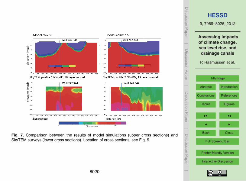
HESSD9, 7969–8026, 2012


P. Rasmussen et al.

Title Page



Tables Figures

J I

J I

Back Close

Full Screen / Esc



Discussion

Paper

|D

iscussionP

aper|

Discussion

Paper

|D

iscussionP

aper|

Fig. 7. Comparison between the results of model simulations (upper cross sections) andSkyTEM surveys (lower cross sections). Location of cross sections, see Fig. 5.

8020





HESSD9, 7969–8026, 2012


P. Rasmussen et al.

Title Page



Tables Figures

J I

J I

Back Close

Full Screen / Esc



Discussion

Paper

|D

iscussionP

aper|

Discussion

Paper

|D

iscussionP

aper|

Lith

olog

y

Natural Gamma(API)0 100

Form. Cond.(mS/m)0 500

Form. Resist.(Ohmm)0 50

Caliper(mm)0 500

Inflow when Q>0(%)0 100

Fluid Cond.(mS/m)0 2000

Fluid Temperature(DegC)8 14

Inflow / advection-diffusion zones and [Cl]

0

-20

-40

-60

-80

-100

sandy layer between clay tills with[Cl] of 650 mg/Lapprox. final 25 % of total inflow<---occurs just below the casingin freshwater advection zone ofthe chalk with measured [Cl] around 200 mg/L

Partly flushed advection zonewith [Cl] around 250 mg/L

<-- approx. 50 % of total inflowoccurs at this level

with [Cl] increasing from 250 mg/Lmixed advection/diffusion controlled zone

to concentrations of the Baltic Sea( approx. 4.4 g/L)

<-- approx. initial 25 % of totalinflow occurs at this level

Saline diffusiive zone with [Cl] abovethe Baltic Sea and approachingocean water (19 g/L) at an estimateddepth of 150 m below surface(~ below the current sea level)

Elev

atio

n (m

asl)

Fig. 8. Results of the geophysical borehole logs from the new deep investigation well (well no.344).

8021





HESSD9, 7969–8026, 2012


P. Rasmussen et al.

Title Page



Tables Figures

J I

J I

Back Close

Full Screen / Esc



Discussion

Paper

|D

iscussionP

aper|

Discussion

Paper

|D

iscussionP

aper|

[

##

#

#

#

#

##

#

#

#!

!.

1

0

2

3

1.5

0.5

-1

-0.5

2.5

-1.5

-2

-2

1.5

-0.5

01

0.5

2

-1

-1

0

0

-0.5

-1.5

Head, layer 7 (m a s l)

Model Row 62

[ Pumping Station

Coastline, canals, streams

!. Well no. 344

! Well no. 172

# Well no. 212

# Abstraction wells

0 1 20.5

Kilometers

¯

a)

b)

c)

Fig. 9. (a) Groundwater head for main chalk aquifer 2010 situation, (b) flow velocity vectorsfor cross section model row 62 (see a), (c) measured groundwater head versus modeled headvalues.

8022





HESSD9, 7969–8026, 2012


P. Rasmussen et al.

Title Page



Tables Figures

J I

J I

Back Close

Full Screen / Esc



Discussion

Paper

|D

iscussionP

aper|

Discussion

Paper

|D

iscussionP

aper|

0.0

0.5

1.0

1.5

2.0

1960 2010 2060 2110 2160 2210 2260 2310

TDS

(g/l

)

Well no. 242.172

SC-0 SC-1 SC-2 SC-3 SC-4

SC-5 SC-6 SC-7 SC-8

0.0

0.5

1.0

1.5

2.0

1960 2010 2060 2110 2160 2210 2260 2310

TDS

(g/l

)

Well no. 242.212

SC-0 SC-1 SC-2 SC-3 SC-4

SC-5 SC-6 SC-7 SC-8

Fig. 10. Model simulation of TDS concentrations (g l−1) in two groundwater abstraction wells for9 scenarios (Table 2).

8023





HESSD9, 7969–8026, 2012


P. Rasmussen et al.

Title Page



Tables Figures

J I

J I

Back Close

Full Screen / Esc



Discussion

Paper

|D

iscussionP

aper|

Discussion

Paper

|D

iscussionP

aper|

Fig. 11. Simulated freshwater-saltwater distribution in 2300 (scale TDS (gl−1)), (a) Basic sce-nario 0, cross section with pumping wells and flow velocity vectors (row 62), (b) basic scenario0, cross section with no pumping and flow velocity vectors (row 68), (c) reference scenario1, cross section with pumping wells (row 62), (d) reference scenario 1, cross section with nopumping (row 62), (e) scenario 1− scenario 0, difference in TDS (mgl−1), cross section withpumping wells (row 62), (f) scenario 1− scenario 0, difference in TDS (mgl−1), cross sectionwith no pumping (row 68).

8024





HESSD9, 7969–8026, 2012


P. Rasmussen et al.

Title Page



Tables Figures

J I

J I

Back Close

Full Screen / Esc



Discussion

Paper

|D

iscussionP

aper|

Discussion

Paper

|D

iscussionP

aper|

Elev

atio

n (m

asl)

0 1000 2000 3000 4000 5000 6000 7000Distance (m)

-100

-80

-60

-40

-20

0E

leva

tion

(mas

l)

0 1000 2000 3000 4000 5000 6000 7000Distance (m)

-100

-80

-60

-40

-20

0

Ele

vatio

n (m

asl)

Fig. 12. Difference in simulated freshwater-saltwater distribution in 2300 (scale TDS, g l−1), (a)scenario 3− scenario 1, cross section with pumping wells (row 62), (b) scenario 3− scenario1, cross section with no pumping (row 68), (c) scenario 6− scenario 1, cross section withpumping wells (row 62), (d) scenario 6− scenario 1, cross section with no pumping (row 68),(e) scenario 8− scenario 1, cross section with pumping wells (row 62), (f) scenario 8− scenario1, cross section with no pumping (row 68).

8025





HESSD9, 7969–8026, 2012


P. Rasmussen et al.

Title Page



Tables Figures

J I

J I

Back Close

Full Screen / Esc



Discussion

Paper

|D

iscussionP

aper|

Discussion

Paper

|D

iscussionP

aper|

-80

-60

-40

-20

0

3000 4000 5000 6000 7000

Ele

vati

on

(m

asl)

Distance (m)

Fig. 13. Flow vectors for scenario 3 in year 2300, model row 62 with two pumping wells. Zoomin on the eastern freshwater lens. Logarithmic flow vector scale and exaggerate vertical velocityflow vectors are used.

8026





Documents

Assessing impacts of climate change, sea level rise, and drainage canals on saltwater intrusion to coastal aquifer