The Income Trajectories of College-Educated Families Living

The Income Trajectories of College-Educated Families Living In or Near Poverty:

Assessing Predictors and Outcomes in Two National Datasets

by

Lauren A. Tighe

A dissertation submitted in partial fulfillment

of the requirements for the degree of

Doctor of Philosophy

(Social Work and Psychology)

in The University of Michigan

2019

Doctoral Committee:

Professor Pamela Davis-Kean, Co-Chair

Professor Larry M. Gant, Co-Chair

Professor Toni C. Antonucci

Professor Andrew Grogan-Kaylor

Lauren A. Tighe

[email protected]

ORCID iD: 0000-0001-7177-3770

© Lauren A. Tighe 2019

ii

DEDICATION

To my late grandfather, Paul "Poppy" Adams, who taught me to work hard and laugh often.

iii

ACKNOWLEDGEMENTS

This dissertation would not be possible without a significant number of individuals. I

owe much of who I am today to these people.

I would first like to thank Dr. Kira Birditt, who took a chance on a freshman who did

not have a clue about research. We have worked together for over a decade and I continue to

grow due to your excellent mentorship, patience, and sense of humor in the somewhat dry

world of academia.

This dissertation, and my graduation from the Joint Doctoral Program, would not

have been possible without my developmental psychology advisor, Dr. Pamela Davis-Kean.

Pam, thank you for always believing in me and my research and skills, especially at times

when I did not believe in myself. This dissertation is so much stronger because of your

feedback and suggestions. This dissertation also benefited from the guidance of my social

work advisor, Dr. Larry Gant. Larry, thank you for showing me the world of program

evaluation and thank you for being flexible and open with the craziness of the joint

program!

I am also very grateful for the support of my additional committee members, Dr.

Toni Antonucci and Dr. Andrew Grogran-Kaylor. Toni, thank you for your years of sage

advice and for challenging me even when I resisted. I have learned so much from you, thank

you for every opportunity. Andy, thank you for always making time for me, staying calm,

and finding solutions when I thought there were none. I love your approach to teaching and

have benefited immensely from your statistics courses.

iv

I thought I had all the friends I needed until I came back to Michigan for graduate

school and met so many wonderful people. First to my Ladies Unchained: Paige Safyer and

Morgan Jerald. I cannot imagine my experience in grad school without you and our weekly

chain restaurant meals, dart playing, and bowling. Paige, it has been a pleasure dining, and

complaining, with you over the past six years. I hope one day you will reconsider our best

friend status but until then you will remain in my phone as "Paige Dog Friend". Morgan, I

look up to you so much for your scholarship and your thoughtfulness, which I hope to

emulate one day. What is LIFEspan development? Next to the text chain thread revolving

around Kanye, Taco Bell, and RBG: Aixa Marchand and Tissyana Camacho. Thank you

both for the laughs and puzzles during grad school, especially when we attempted to find

Rihanna's new album on YouTube. Aixa, thank you for befriending me during SI and

remaining on the taco hunt with me all these years. Tiss, thank you for being the older, more

experienced grad student mentor I needed especially during the dissertation analys is

process. To the "Fam": Neelima Wagley, Jack Wong, Maria Schmieder, and Abhi Nikam. I

will always remember our minivan adventures, Movement weekends, and LIVE nights. You

were an invaluable source of relief and fun away from academia. Thank you to my friend

and ISR office mate for many years, Jasmine Manalel. Jasmine, I think back fondly of all

our times laughing, complaining, and searching for free food around the building. Thank

you to my friend and lab mate, Alexa Ellis. Alexa, lab was so much fun when were together

especially when we attempted that women in STEM project. On to the next gluten-free

adventure! Next to my friend and amazing doctor-to-be, Nina Fabian. We have been friends

for so long, ever since we rode a yellow school bus every day from Queens to Harlem in the

hottest summer in NYC history. Visiting Detroit offered a much-needed respite from

v

Ann Arbor and work and I treasure all of our memories and afternoons eating pie. Lastly, to

Alex Gross who has stood by me and offered support even in my most intolerable moments.

Alex, I don't know how you do it but thank you for always staying positive and resisting the

urge to fight fire with fire. I am excited that we are on this journey together.

I was scared to join not one, but two, cohorts of completely random graduate

students when I started the Joint Doctoral Program but was so lucky to make such amazing

friends. Thank you to the 2013 Developmental Psychology cohort for your feedback over

the years and support during the dissertation process: Sammy Ahmed, Nkemka Anyiwo,

Emma Beyers-Carlson, Kim Brink, Fernanda Cross, Margaret Echelbarger, Arianna Gard,

Amira Halawah, Tyler Hein, Jasmine Manalel, and Neelima Wagley. Thank you to the 2013

Social Work cohort for your thoughtfulness and reminders on why we do this work:

Nkemka Anyiwo, Finn Bell, Peter Felsman, Angie Perone, Taha Rauf, Lauren Whitmer, and

Pinghui Wu.

Thank you so much to all the members of the Human Development Quantitative

Methods lab for your feedback on ideas, presentations, and manuscripts. Your comments on

my dissertation increased its rigor and thoughtfulness on complicated issues. Thank you to

all of the members of the Life Course Development lab for your feedback and opportunities

to grow with a special thanks to Angela Turkelson. Angie, thank you for always making

time for me to ask questions about statistics, even though most of them had obvious

answers, and for always being a friendly face in a crowd.

No dissertations would be possible without the constant work of the administrative

teams. Thank you to Brian Wallace and Sarah Wagner in the Psychology Student Academic

Affairs office and Todd Huynh and Laura Thomas in the Joint Doctoral Program office.

vi

Thank you for working with me even when I presented some difficult challenges and I truly

appreciate everything you have done for me. Thank you to Dr. Berit Ingersoll -Dayton, the

past director of the Joint Program. Berit, thank you for your constant kindness. You have a

way of making people, especially lowly grad students, feel important and I thank you for all

of our conversations. I would also like to thank the Institute for Social Research, a place I

have called home since 2007, and Dr. Robert Kahn for their generosity in providing support

for my dissertation.

Lastly, thank you to my family: my mother, Debra Adams-Tighe, and my brother,

Michael Tighe. We have faced significant challenges, but together we are a stronger family.

I love you.

vii

TABLE OF CONTENTS

DEDICATION ii

ACKNOWLEDGEMENTS iii

LIST OF TABLES ix

LIST OF FIGURES xiii

LIST OF APPENDICES xiv

ABSTRACT xv

CHAPTER

I. Introduction 1

The Achievement Gap, Parental Education, and Family Income 2

Statement of the Problem 5

Significance of the Study 6

Dissertation Study Overview 6

II. Literature Review 8

Theoretical Framework 8

Parental Education and Achievement 13

Family Income and Achievement 17

Poverty Duration over Time 20

viii

Sociodemographic Characteristics of Families Experiencing Transient and Chronic Poverty 22

Later Outcomes of Families Experiencing Transient and Chronic Poverty 25

Research Aims and Hypotheses 26

III. Method 30

Participants 30

Measures 32

Analysis Strategy 45

IV. Results 50

Research Question 1: Identification of Income Status Trajectories 50

Research Question 2: Predictors of Income Status Trajectories 51

Research Question 3: Distal Outcomes Predicted by Income Status Trajectories 52

Research Question 4: Replication and Extension 54

Post Hoc Analyses 56

Sensitivity Analyses 58

Power Analyses 65

V. Discussion 68

Diverse Experiences of Low-income, Highly-educated Families over Time 68

Sociodemographic Characteristics Linked to Longer Durations of Economic Hardship 73

Issues of Methodology and Comparisons across Datasets 86

Limitations and Future Directions 90

Conclusion 99

APPENDICES 133

REFERENCES 146

ix

LIST OF TABLES

TABLE

Table 1 102

Original Analyses: ECLS-K: 1998 102

Descriptives of Low-Income, Highly-Educated Families at Kindergarten in ECLS-K: 1998 102

Table 2 103

Replication Analyses: ECLS-K: 2010 103

Descriptives of Low-Income, Highly-Educated Families at Kindergarten in ECLS-K: 2010 103

Table 3 104


Fit Indices for ECLS-K: 1998 Income Status Trajectory Classes (N = 540) 104

Table 4 105


Trajectory Results in Probability Scale for ECLS-K: 1998 105

Table 5 106


Descriptives of ECLS-K: 1998 Trajectories at Kindergarten 106

Table 6 107


Sociodemographic Predictors of Income Status Trajectory Membership in ECLS-K: 1998 (n =

375) 107

Table 7 108


Differences in Distal Outcome Means between Trajectory Classes in ECLS-K: 1998 (N = 540)

108

Table 8 109



x

Table 9 110



Table 10 111


Descriptives of ECLS-K: 2010 Trajectories at Kindergarten 111

Table 11 112



354) 112

Table 12 113



113

Table 13 114

Post hoc analyses: Descriptives 114

Means and Standard Deviations of Distal Outcomes by Income and Education Family Types in

the ECLS-K: 1998 114

Table 14 115

Post hoc analyses: Descriptives 115

Means and Standard Deviations of Distal Outcomes by Income and Education Family Types in

the ECLS-K: 2010 115

Table 15 116

Sensitivity Analyses: Dataset Differences 116

Fit Indices for ECLS-K: 1998 Income Status Trajectory Classes (n = 537) 116

Table 16 117



Table 17 118


Fit Indices for ECLS-K: 2011 Income Status Trajectory Classes (n = 417) 118

Table 18 119

xi



Table 19 120



373) 120

Table 20 121



327) 121

Table 21 122



122

Table 22 123


Differences in Distal Outcome Means between Trajectory Classes in ECLS-K: 2011 (N =417)

123

Table 23 124

Sensitivity Analyses: Data Collection Intervals 124


Table 24 125

Sensitivity Analyses: Data Collection Intervals 125


Table 25 126

Sensitivity Analyses: Multiple Imputation 126

Sociodemographic Predictors of Income Status Trajectory Membership in ECLS-K: 1998 (N =

540) 126

Table 26 127

Sensitivity Analyses: Multiple Imputation 127

Sociodemographic Predictors of Income Status Trajectory Membership in ECLS-K: 2010 (N =

449) 127

xii

Table 27 136

Thresholds for 1998 (Wave 2, Kindergarten) 136

Table 28 136

Thresholds for 1999 (Wave 4, First Grade) 136

Table 29 137

Thresholds for 2001 (Wave 5, Third Grade) 137

Table 30 137

Thresholds for 2003 (Wave 6, Fifth Grade) 137

Table 31 137

Thresholds for 2006 (Wave 7, Eighth Grade) 137

Table 32 138

Thresholds for 2010 (Wave 2, Kindergarten) 138

Table 33 138

Thresholds for 2011 (Wave 4, First Grade) 138

Table 34 139

Thresholds for 2012 (Wave 6, Second Grade) 139

Table 35 139

Thresholds for 2013 (Wave 7, Third Grade) 139

Table 36 139

Thresholds for 2014 (Wave 8, Fourth Grade) 139

Table 37 140

Thresholds for 2015 (Wave 9, Fifth Grade) 140

xiii

LIST OF FIGURES

FIGURE

1. ECLS-K: 1998 income status trajectories over time 128





xiv

LIST OF APPENDICES

APPENDIX

A. Income category codes in ECLS-K: 1998 134

B. Income category codes in ECLS-K: 2011 135

C. Low-income thresholds for ECLS-K: 1998 136

D. Low-income thresholds for ECLS-K: 2010 138

E. Parent occupation codes for ECLS-K: 1998 and ECLS-K: 2010 141

F. Fifth grade distal outcome measures for ECLS-K: 1998 sensitivity analyses 143

xv

ABSTRACT

The relationship between parental education and family income to parenting practices

and children’s achievement is well-documented. The effects of high parental education on these

behaviors in the face of financial difficulty over time, however, are less established. Therefore,

this study seeks to examine the longitudinal income status trajectories of low-income, highly-

educated families in addition to the predictors and outcomes of experiencing varying durations of

economic hardship. The first research aim identified income status trajectories of college-

educated families living in or near poverty. The second research aim determined whether

sociodemographic characteristics, such as race or sex, predict to different durations of economic

hardship. The third research aim examined the effect of different durations of economic hardship

on distal parent and child outcomes. The last research aim attempted to replicate findings in a

conceptually similar dataset.

Two datasets were used to investigate these research aims: Early Child Longitudinal

Study 1998-99 (ECLS-K: 1998) and the Early Childhood Longitudinal Study 2010-11 (ECLS-K:

2010). To be included in the analyses, families must be low-income (i.e., living at or below

200% of the federal poverty line) and have at least one parent with a college degree (i.e.,

Bachelor’s degree or higher) when their child was in kindergarten. Families must also have

participated in at least two waves of data following kindergarten (ECLS-K: 1998 N = 540;

ECLS-K: 2010: N = 449). First, latent growth curve analyses (LCGA) in Mplus identified

income status trajectories. Second, multinomial logistic regressions determined predictors of the

xvi

previously identified latent trajectories. Last, mean equality tests examined distal outcome

differences amongst the previously identified latent trajectories. These three analyses were first

conducted in the ECLS-K: 1998 and then replicated in the ECLS-K: 2010.

In the ECLS-K: 1998, two trajectories emerged: Transient (i.e., above the low-income

threshold in most waves) and Chronic (i.e., at or below the low-income threshold in most

waves). Compared to the Transient class families, the Chronic class families were more likely to

have a parent identify as Black and live in rural areas and less likely to have a parent with an

occupation requiring a postsecondary degree. Parents in the Transient class reported higher

school involvement, satisfaction with their child’s school, and warmth towards their child and

children in the Transient class had higher reading and math achievement compared to families in

the Chronic class. In the ECLS-K: 2010, three trajectories emerged: Immediate Transient (i.e.,

immediately above the low income threshold in most waves), Delayed Transient (i.e., initially at

or below the low-income threshold but gradually rose above it over time), and Chronic (i.e., at or

below the low-income threshold in most waves). No sociodemographic characteristics predicted

trajectory class membership. Parents in both the Delayed Transient and Chronic classes reported

more rules in the household than parents in the Immediate Transient class.

This study was one of the first to investigate income trajectories in low-income, highly-

educated families over time. Variation in duration of poverty sociodemographic characteristics

and outcomes amongst low-income, college-educated families highlight the need for a range of

policy and program solutions to address diverse familial needs. Parental education may be a

protective buffer for parents and children in the face of economic hardship. The difference in

results between the two datasets suggests issues of historical validity and additional sensitivity

analyses identified important methodological differences when comparing across datasets.

1

CHAPTER I

Introduction

Former president Barack Obama called the growing economic inequality and lack of

social mobility in the United States “the defining challenge of our time” (Obama, 2013). The

United States is simultaneously one of the richest countries in the developed world and one of

the most unequal (Stiglitz, 2012). In 2016, over 40 million Americans experienced poverty with

even more living precariously close to the poverty line (Semega, Fontenot, & Kollar, 2017).

Behind growing economic inequality, social mobility has remained stagnant for decades (Katz &

Krueger, 2017). A recent study by Chetty and colleagues (2014) found that children growing up

in America today are no more economically mobile than children born 50 years ago. Research

also shows stability in social mobility such that children from high-income families will likely

stay wealthy while children from low-income families will likely remain poor (Greenstone,

Looney, Patashnik, & Yu, 2013). In response to the growing inequality and decreasing mobility,

Nobel-prize winning economist Joseph Stiglitz (2012) declared the “American Dream”, the

belief that any American who works hard can be successful due to equal opportunity and upward

mobility, to be a myth.

Education is often seen as the primary source of upward mobility in the United States and

is championed as a way to lift people out of poverty (Hershbein, Kearney, & Summers, 2015).

To be sure, attaining a higher education often leads to further financial success (Hout, 2012; Ma,

Pender, & Welch, 2016), but it is not a guarantee. In 2016, approximately 3.3 million college-

2

educated adults lived in poverty (Semega et al., 2017). And in 2015, 15 million children lived in

low-income families where one parent had at least some college education (Jiang, Granja, &

Koball, 2017). Yet, little is known about these children, parents, and families at the intersection

of income and education. By examining families that are low-income (i.e., in or near poverty)

but highly educated (i.e., Bachelor’s degree or higher), important insights can be gained into how

these specific mechanisms operate, influence academic achievement and behavior, and provide

potential pathways to confront inequality.

The Achievement Gap, Parental Education, and Family Income

Research on the achievement gap, the large disparities in academic outcomes between

different groups of students, has garnered significant attention in recent years (Reardon, 2011).

During his term as president, Obama described education equality as a civil rights issue

(Tavernise, 2012) and announced numerous initiatives such as ‘My Brother’s Keeper’ and

‘Generation Indigenous’ to improve achievement and increase resources and opportunities for

children of color (The White House, 2014; U.S. Department of Education, 2016). With this in

mind, Reardon (2011) found that the achievement gap between White and Black students has

actually decreased over time. Meanwhile, the achievement disparities between children from

low-income families and children from high-income families have grown larger. Reardon (2011)

estimated that the income achievement gap sharply increased by approximately 40% from the

1970’s to 1990’s. The income achievement gap is already apparent when children begin formal

schooling in kindergarten (Duncan & Magnuson 2011; Lacour & Tissington, 2011; Reardon,

2011), with children from low-income families scoring lower on assessments compared to

children from high-income families (Aikens & Barabin, 2008; Duncan & Magnuson, 2011). This

3

gap does not significantly narrow from fall to spring of kindergarten and persists as children go

through school (Duncan & Magnuson, 2011; Reardon & Portilla, 2016).

Recent evidence suggests the income achievement gap is slowly decreasing, but Reardon

(2016) posits that it will take between 60 and 110 years to completely eliminate the achievement

gap at its current rate of decline. Many interventions and programs designed to expand

opportunities for less advantaged children are aimed at improving teacher or school quality

(Bower, 2013). But children only spend approximately six hours, or one-fourth, of the day in

school and the remaining time is spent in the home environment with their parents and families.

Consequently, the context of the family and home environment is extremely relevant when

studying achievement and educational inequalities. Examining families’ socioeconomic status

may provide useful insights into the specific, and unique, mechanisms of parental education and

family income on children’s achievement as well as parenting practices and behaviors.

Two aspects of families’ socioeconomic standing, parental education and family income,

are well-established direct and indirect predictors of children’s academic achievement. Parents’

education is strongly linked to children’s achievement and educational attainment (Dubow,

Boxer, & Huesmann, 2009; Magnuson & McGroder, 2002; Magnuson, Sexton, Davis-Kean, &

Huston, 2009). Davis-Kean (2005), for example, found strong parental education effects, both

directly and indirectly, for young children’s achievement. Davis-Kean and others have found that

parental education indirectly influences children’s achievement through parental educational

expectations, reading behavior in the home, and warmth in the parent-child relationship (Davis-

Kean, 2005; Englund, Luckner, Whaley, & Egeland, 2004; Hoffman, 2003; Kim & Rohner,

2002; Klebanov, Brooks-Gunn, & Duncan, 1994; Zheng & Libertus, 2018). Research also

suggests mothers with higher education have more diverse and complex language, engage in

4

more developmentally appropriate activities, and devote more resources to child enrichment

expenditures compared to mothers with less education (Kalil, Ryan, & Corey, 2012; Kaushal,

Magnuson, & Waldfogel, 2011; Rowe, Pan, & Ayoub, 2005)

Similarly, the effects of family income on achievement is well-documented (Duncan,

Morris, & Rodrigues, 2011; Hill & Duncan, 1987; Lacour & Tissington, 2011) with children

from lower income families typically performing more poorly on standardized achievement tests

compared to children from higher income families (Smith, Brooks-Gunn, & Klebanov, 1997).

Income has also been found to be an important indirect influence on the home environment,

parenting style, and the availability of resources for the child (Brooks-Gunn & Duncan, 1997;

Duncan et al., 2011; Fox, Platz, & Bentley, 1995; Guo & Harris, 2000; McLoyd, 1998; Smith et

al., 1997). For example, Guo and Harris (2000) found that income affects parental stressors that,

in turn, influence parental warmth and discipline. In terms of resources, Kauhshal et al. (2011)

found that parents with higher incomes spend significantly more on enrichment activities or

private school tuition for their child than parents with lower incomes.

Although education and income demonstrate unique effects on children’s achievement

(Duncan & Magnuson, 2001, 2005), research often uses samples where education and income

are moderately and positively related (i.e., low education and low income or high education and

high income; Huston & Bentley, 2010; Smith et al., 1997). Thus, it is difficult to disentangle

their distinct influences on achievement due to correlating, and potentially confounding, factors.

Research by Tighe and Davis-Kean (under review) attempted to disentangle the relation by

studying low-income, college-educated families and found that children from these families

scored significantly higher on reading and math tests compared to children from both low-

income, less-educated and high-income, less-educated families. Low-income, highly-educated

5

parents were also more likely to engage in educational activities with their child, such as going to

libraries and museums, compared to high-income, less-educated parents (Tighe & Davis-Kean,

under review). These findings demonstrate the distinct influence of higher education, which may

provide a buffering effect against the negative effects of living in or near poverty.

Statement of the Problem

Low-income, highly-educated families are growing in the United States yet are

underrepresented in the research on children, families, and achievement. Research on low-

income families often assumes these families are similar while ignoring the existing

heterogeneity. Previous work has examined low-income, highly-educated families in contrast to

other types of families (Tighe & Davis-Kean, under review) but important differences may exist

within this subgroup. Furthermore, research on families in or near poverty typically only

captures one year of income which can seriously underestimate the relationship between income

and children’s cognitive test scores (Mayer, 1997; Michelmore & Dynarski, 2017). Research has

found significant differences in achievement and behavior in kindergarten for children from low-

income, highly-educated families (Tighe & Davis-Kean, under review), but less is known about

whether the buffering effect of parental education can persist over time. Therefore, studying

families longitudinally can capture stability, or instability, in a family’s income that may

influence parenting practices and children’s achievement (Katz, Corlyon, La Placa, & Hunter,

2007). Moreover, measuring income longitudinally and considering differences between

transient and chronic poverty has not been applied as extensively in the United States as other

countries (Kimberlin, 2016).

6

Significance of the Study

One approach to promote children’s academic success considers the possible protective

effects of parental education when the family lacks financial resources. This dissertation study

examines the influence of changing income status from early to middle childhood on a variety of

outcomes. For example, this study sheds light on which children score highly on achievement

assessments and possible parenting practices (e.g., setting family rules, engaging in educational

interactions) that may affect achievement. This study also illuminates sociodemographic

inequalities in income patterns over time in whether families are experiencing only a brief stint

in or near poverty or are experiencing long-term economic hardship. Answering these questions

will help researchers, policymakers, social service programs, teachers, and schools understand

and provide support for families that may have unique needs. The findings from this dissertation

provide empirical evidence regarding diversity within low-income populations and the effects of

high parental education which could dispel myths and stereotypes about which types of

Americans live in or near poverty.

Dissertation Study Overview

The present dissertation study seeks to examine the rich diversity of college-educated

families that are living in or near poverty using two nationally-representative and conceptually

similar datasets. First, this study acknowledges the changing income of many families living in

or near poverty and seeks to identify income status trajectories of families using growth curve

modeling in a sample from the late 1990’s. Next, sociodemographic differences in trajectory

membership will be investigated to further dissect the nuances of each trajectory and possible

reasons for belonging to each income trajectory. This study then examines children’s later

reading and math achievement outcomes based on their identified family income trajectory.

7

Furthermore, parental behaviors and family context that may be influential to children’s

achievement will also be examined. Lastly, the family income trajectories and patterns identified

will be compared to trajectories from a more contemporaneous sample collected in the 2010’s,

providing empirical evidence for its replicability. Overall, this study seeks to further understand

these families and whether high parental education can attenuate the effects of economic

hardship through children’s academic achievement and associated parenting practices and

behaviors.

8

CHAPTER II

Literature Review

This dissertation focuses on families living in or near poverty (e.g., families who are low

income but are not necessarily at or below the federally-defined poverty thresholds). While the

bulk of the literature refers specifically to poverty, these same theories or empirical findings may

also apply to families that are considered low-income but not necessarily living in poverty.

Because of possible similarities, literature that focuses on poverty along with income more

broadly will be discussed.

Theoretical Framework

“Poverty does not and should not define a person or group of people – there is no

“culture of poverty” – but it can define a stratified system in which a person or group of people

may live” (Milner, 2015, p. 13).

In 1959, Oscar Lewis published Five Families: Mexican Case Studies in the Culture of

Poverty describing families living in poverty in Mexico. Based on his observations, he

concluded that people living in poverty develop values and behaviors that are different than the

rest of the population (Lewis, 1959, 1966). He argued that this poverty-perpetuating value

system is then passed on from parents to children through socialization, making it difficult or

impossible for low-income families to leave their situation. The culture of poverty thesis assumes

low-income families are homogenous in nature (Salcedo & Rasse, 2012). It posits that parental

involvement and child outcomes, such as academic achievement, vary between social classes

9

because lower class parents place less emphasis or value on schooling (Lareau, 1987). Further,

the culture of poverty perspective assumes that low-income parents are so entrenched in poverty

culture that any increases in income will not lead to changes in values or behaviors (Lewis, 1966;

Mayer, 1997).

Many researchers have rejected the culture of poverty thesis, along with its assumption of

homogeneity, by identifying different behaviors, expectations, and outcomes among individuals

and families living in similar economic conditions (Anderson, 1999; Hannerz, 1969; Ho &

Willms, 1996; Small, Harding, & Lamont, 2010). One of the most common criticisms of the

culture of poverty thesis is that it fails to differentiate individuals’ behavior from their values and

beliefs (Lamont & Small, 2008). Research suggests that low-income individuals and families

hold many middle-class values but their disadvantaged circumstances make it difficult to behave

according to their values. For example, Edin and Kefalals (2005) interviewed low-income Black

women and found, overall, that the women valued marriage and raising children in a two-parent

household but had difficulty realistically achieving this goal. Another criticism is that the culture

of poverty perspective allows for the poor to be blamed for their economic conditions (Small et

al., 2010). Specifically, the culture of poverty has been primarily used to describe Black

Americans, rather than the entire American population (Peterson, Maier, & Seligman, 1993;

Salcedo & Rasse, 2012; Wilson, 2009). Assistant Secretary of Labor, Patrick Moynihan, used the

culture of poverty as a basis for his influential report on the “pathologies” of Black Americans in

poverty which critics argue diverts responsibility for poverty from larger structural factors to the

individual behaviors of the poor (Ryan, 1976; Small et al., 2010). In response, more recent

scholars have maintained that explanations of poverty must consider the interaction between

structural factors and individual characteristics (Bourgois, 2001; Small et al., 2010). These

10

conditions and experiences affect an individual’s range of choices and pathways (Lamont &

Small, 2010). Rather than focusing on deficits, this dissertation considers a strengths-based

approach, typically used in social work practice, to examine low-income families and their

behaviors.

A strengths-based perspective accounts for what individuals and families know and what

they can do by considering their knowledge, resources, capacities, values, and beliefs (Saleebey,

1996). This strengths-based perspective is most often used in individual case management but

can be applied to family systems more broadly. In fact, Hartman (1981) described families as

“the primary social service agency in meeting social, educational, and health care needs” (p. 10).

Families often have resources that will help meet their child’s educational needs, such as in this

study’s sample of families who have obtained a college education. The strengths-based

perspective does not ignore the very real challenges facing families, such as economic stressors,

but prioritizes identifying positive strengths that can be harnessed for change (Ronnau &

Poertner, 1993; Saleeby, 1996).

García Coll and colleagues (1996) proposed a theoretical model of child development

that considers both social position and social stratification at the core of its framework. Focusing

primarily on race and ethnicity, they critiqued previous research that failed to analyze intragroup

variability and emphasized between group differences. They urged mainstream models to

simultaneously incorporate multiple important sources of influence (García Coll et al., 1996).

While this dissertation study does not place significant emphasis on race, the critiques of García

Coll et al. (1996) can be applied to theories of social class. Indeed, much of the developmental

psychology and social work theory literature focuses solely on either education or income,

without considering the unique contribution of each. Davis-Kean (2005), however, suggested a

11

conceptual model that incorporates both direct and indirect paths of parental education and

family income on parenting capacity and children’s achievement. This conceptual model that

examines both the relation with parent education and family income will be used to guide this

study’s research aims, hypotheses, and interpretation of findings. The following theoretical

frameworks on parenting and child development inform various aspects of the Davis-Kean

(2005) model, particularly the direct and indirect links between family income, parental

behaviors, and children’s achievement.

First, investment theory, or human capital theory, posits that parents invest time and

money into “human capital.” The theory holds that parents invest finances in education and other

goods or services that will, in turn, improve their child’s future well-being (Becker, 1991, 1994;

Becker & Tomes, 1986). It also proposes that these investments are influenced by parental

preferences, such as the importance placed on education, along with tangible resources.

Investment theory suggests that children from affluent families will be more likely to succeed

than children from low-income families because wealthier families have more money to invest in

resources and services. Low-income parents may not be able to afford cognitively stimulating

resources, such as books and educational materials, or high-quality schools and safe

neighborhoods. Additionally, low-income parents may be unable to devote as much time to their

child due to long or odd work hours or a less flexible work schedule (Duncan, Magnuson, &

Votruba-Drzal, 2017).

Second, parental and family stress theory recognizes that experiencing poverty is stressful

and that stress can increase marital instability and decrease parents’ ability to be supportive and

involved with their children (Conger et al., 1992; Conger, Ge, Elder, Lorenz, & Simons, 1994;

McLoyd, 1990, 1998). Families struggling with economic hardship usually experience other

12

stressful life events that create psychological distress and hostile feelings which can spread to

parenting practices (Kessler & Cleary, 1980, McLeod & Kessler, 1990). Elder’s studies of White

families during the Great Depression found that fathers who experienced significant financial

loss were more irritable, tense, and prone to punitive parenting which predicted children’s

socioemotional problems (Elder, Liker, & Cross, 1984; Elder, Nguyen, & Caspi, 1985). McLoyd

(1990) posited that this type of insensitive and unsupportive parenting has serious consequences

for children that are ultimately detrimental to a number of developmental outcomes. Recent

research has replicated these findings in more diverse populations such as single-parent families

or ethnically diverse urban families (Brody & Flor, 1997; Conger, Wallace, Sun, Simons,

McLoyd, & Brody, 2002; Mistry, Vandewater, Huston, & McLoyd, 2002; Parke et al., 2004;

Solantaus, Leinonen, & Punamäki, 2004).

Although the links between parental education, parent’s behaviors, and children’s

achievement are established, there lacks a rich theoretical framework for the important influence

of parental education. Harding, Morris, and Hughes (2015) propose a framework based on

capital, bioecological, and developmental niche theories. First, the authors argue that as maternal

education increases so does mothers’ access to various forms of capital, such as human, cultural,

and social capital, that shapes parenting practices. There is a specific focus on parenting practices

as the unique mechanisms of maternal education on children’s academic development after

accounting for other common components of socioeconomic status. These parenting practices do

not happen in isolation but instead occur throughout various levels of a parent and child’s

ecological environment (e.g., microsystem, exosystem; see Bronfenbrenner & Morris, 2006).

Last, developmental niche theory suggests that children’s academic outcomes are improved by

mothers’ systematic and repetitive behavioral patterns in which “the mechanisms associated with

13

maternal education reinforce each other to influence children’s academic outcomes” (Harding et

al., 2015, p. 63).

Although some developmental theories acknowledge the diversity of families, many do

not. These theoretical frameworks provide a useful guide towards understanding the nuances and

consequences of income and education for parent and child outcomes, but they may not

necessarily describe the behaviors of low-income, highly-educated parents. For example,

Becker’s investment theory suggests that low-income parents do not have the resources, or

capital, to provide rich educational environments for their children. At the same time, Harding et

al.’s (2015) maternal education framework suggests highly-educated mothers have access to

human and social capital that can be routed towards enhancing their children’s development.

When examined alone, these theories appear to describe the behaviors of large segments of the

population. But when applied in tandem to a unique sample – families who live in or poverty

with a college education – the utility of the frameworks is less clear and somewhat contradictory.

Parental Education and Achievement

Family socioeconomic status (SES), typically measured by parents’ education,

occupation type, family income, or wealth, is well-recognized as contributing to education and

achievement disparities. Two highly studied aspects of SES, parental education and family

income, are considered the most powerful explanatory variables of children’s academic

outcomes (Duncan, Kalil, & Ziol-Guest, 2017). And although aspects of SES are interrelated,

each influences children and families through unique mechanisms (Duncan & Magnuson, 2003,

2012). Parental education is strongly related, both directly and indirectly, to children’s

achievement (Davis-Kean, 2005; Dubow et al., 2009; Magnuson & McGroder, 2002; Magnuson

et al., 2009). In a sample of 8- to 12-year-olds, Davis-Kean (2005) found a positive link between

14

parental education and children’s achievement in European American families. Similarly,

Conger et al. (1997) found that mother’s education was positively related to school achievement

in 14- to 17-year-old adolescents.

Interestingly, maternal education remains a statistically significant predictor of young

children’s reading and math achievement scores even when controlling for income (Smith et al.,

1997). A study by Isaacs and Magnuson (2011) found children of mothers with a bachelor’s

degree scored higher on reading and math skills than children of mothers without a college

degree after controlling for a range of covariates including income. More specifically, children

whose mothers had a bachelor’s degree scored 0.37 and 0.32 standard deviations higher in

reading and math, respectively, than children whose mothers did not complete high school

(Isaacs & Magnuson, 2011). Overall, Isaacs and Magnuson (2011) estimated that an additional

year of maternal education would increase academic skills by .06 to .09 standard deviations. And

the researchers posited that an even larger maternal education increase, such as going from a

high school degree to obtaining a bachelor’s degree, would have an even more substantial effect

on children’s school readiness (0.26 to 0.32 standard deviations). The researchers also studied

mothers who increased their education over the course of study and found no effects. Yet other

studies of changes in maternal education after the birth of a child have found positive links to

children’s achievement (Magnuson, 2007). Using propensity score matching in a sample of Head

Start-eligible children, Harding (2015) found that children with mothers who increased their

education scored higher on a number of academic skills compared to children with mothers who

did not increase their education over the course of several years.

Parental warmth has been linked to children’s achievement in a number of studies

(Davis-Kean, 2005; Hoffman, 2003; Kim & Rohner, 2002) with findings suggesting education,

15

not income, predicts parental warmth (Klebanov et al., 1994). Compared to less educated

mothers, highly-educated mothers are more emotionally responsive (Bradley et al., 1989) and

have more positive and less hostile interactions with their child (Fox et al., 1995). Increasing

maternal education after the birth of a child has been linked to increases in the presence of

children’s learning materials as well as maternal responsiveness (Magnuson, 2007). Higher

educated mothers tend to use more complex and rich language in the home with their children

(Hoff, Laursen, & Tardiff, 2002; Hoff, 2003) and engage in more verbal and non-verbal

activities (Suizzo & Stapleton, 2007). Moreover, higher educated, low-income mothers talk more

and use more diverse language compared to less educated, low-income mothers (Rowe et al.,

2005). Highly-educated parents not only spend more time with their children, but also devote

more time to developmentally-appropriate activities (Guryan, Hurst, & Kearney, 2008; Kalil et

al., 2012). Furthermore, evidence suggests parental education level is positively related to

parent’s education expectations for their children (Davis-Kean, 2005; Halle, Kurtz-Costes, &

Mahoney, 1997). Parents with more education tend to have higher expectations for their

children’s educational attainment (Englund et al., 2004; Gill & Reynolds, 1999; Singh, Bickley,

Trivette, & Keith, 1995; Suizzo & Stapleton, 2007).

Highly-educated parents are typically more involved in their child’s education in both the

school and home (Englund et al., 2004; Keith, Keith, Quirk, Cohen-Rosenthal, & Franzese,

1996; Shumow & Miller, 2001; Singh et al., 1995). Mothers with higher education levels attend

more school activities and meetings (Lareau, 2011; Pomerantz, Moorman, & Litwack, 2007).

Further, higher educated mothers provide more educational resources in the home (Bradley &

Corwyn, 2002; Rodriguez et al., 2009) with child enrichment expenditures varying positively

with mother’s education level (Kaushal et al., 2011). Compared to less educated families,

16

families with higher educated mothers spend a larger proportion of their budget on enrichment

such as family trips, computers, books and magazines, school supplies, and recreation activities

(Kaushal et al., 2011). This dissertation not only examines children’s achievement scores, but

considers how highly-educated parents may be indirectly helping their children succeed

academically through parent-child interactions, involvement, and educational expectations.

Yet there are mixed findings as to whether parental behaviors and investments in

children’s activities influence children’s achievement. Parental school involvement has been

shown to positively, but moderately, predict children’s achievement (see Fan & Chen, 2001 or

Hill & Tyson, 2009 for meta-analytic reviews). Some researchers have found that parents’

involvement with their children’s education benefits students, schools, and the parents

themselves (Comer, 2005; Henderson & Mapp, 2002). Lee and Bowen (2006), however,

examined several different types of parent involvement and found that only parent involvement

within schools (e.g., conference attendance, volunteer work) and parent expectations of success

were significantly associated with achievement.

As children age, parents become less involved in formal, school-based activities (e.g.,

volunteering at school) but continue informal, home-based activities (e.g., child has a regular

place to do homework at home; Eccles & Harold, 1996; Epstein, 1986; Epstein & Dauber, 1991).

Some research suggests home-based involvement may be a stronger predictor of achievement

than school-based involvement (Fantuzzo, McWayne, Perry, & Childs, 2004; Ho & Willms,

1996). At-school involvement requires parents to have the time and resources to participate and

teachers and schools may not initiate requests for communication or involvement as children get

older (Eccles & Harold, 1996; Shumow & Miller, 2001). For example, Izzo, Weissberg, &

Kasprow (1999) found a decrease in the frequency of parent-teacher contacts, interactions, and

17

parent participation from kindergarten yet participation in educational activities at home showed

no significant change over time. Furthermore, educational activities at home predicted children’s

(third to fifth grade) reading and math achievement, more than parental school involvement

variables. In a sample of eighth graders, Ho and Willms (1996) found that parent-child

discussions about school activities significantly predicted children’s academic achievement. The

researchers also found virtually no difference in the amount of home supervision (e.g., limiting

television time, monitoring homework) provided by families of different socioeconomic statuses

(Ho & Willms, 1996). Conversely, Lee and Bowen (2006) found that parent support at home

(e.g., helping with homework, discussing educational topics, and managing children’s activities)

was not significantly related to children’s achievement. This study examines parental

involvement at school and home in order to understand what educational resources highly-

educated parents can provide with limited financial resources.

Family Income and Achievement

Family income also has direct and indirect effects on children’s achievement, albeit

weaker than parental education (Davis-Kean, 2005; Lacour & Tissington, 2011; Linver, Brooks-

Gunn, & Kohen, 2002). Beginning in kindergarten, children from low-income families typically

perform more poorly on academic assessments compared to children from higher income

families (Smith et al., 1997; Duncan & Magnuson, 2011; Magnuson & Duncan, 2006). Duncan

& Magnuson (2011) showed that children from the bottom income quintile scored almost one-

and-a-half standard deviations below children from the top income quintile on math assessments.

Using data from the Early Childhood Longitudinal Study (Kindergarten ‘98/99), Reardon (2011)

found that the achievement gap between high- and low-income groups in reading and math

continues from kindergarten to eighth grade. Although this achievement gap persists over time, it

18

does not widen as children go through formal schooling, suggesting unequal school experiences

and resources are not the primary cause (Duncan & Magnuson, 2011; Reardon, 2011).

Although the majority of the research linking family income to children’s achievement is

correlational, causal or quasi-experimental studies have demonstrated the significant effect of

family income. Using data from 16 welfare-to-work experiments, Duncan and colleagues (2011)

found that a sustained $1,000 increase in annual income was associated with 0.06 standard

deviation increase in young children’s achievement. Dahl and Lochner (2012) found similar

results when examining the effect of a policy-induced increase in maximum Earned Income Tax

Credit (approximately $2,000) on children’s school achievement. In a non-experimental study,

Isaacs and Magnuson (2011) found much smaller effects for increasing income with an

additional $1,000 of average income resulting in a 0.015 standard deviation increase in reading

and math scores for low-income families. Akee and colleagues (2011) used a natural experiment

of casino profit disbursement payments to families (approximately $4,000 per year) to examine

the effect of increased income on educational attainment. They found that American Indian

children from families who received these payments had higher educational attainment in young

adulthood than children from non-American Indian families who were not eligible for the

payments. Yet other research on cash assistance for low-income families found annual income

increases (approximately $2,000 per year) had no effect on children’s school progress or

outcomes (Miller et al., 2016).

A number of studies suggest a cognitively stimulating home environment has positive

effects on children’s development and achievement (Brooks-Gunn & Duncan, 1997; Fox et al.,

1995; McLeod & Shanahan, 1993; Smith et al., 1997; Yeung, Linver, & Brooks-Gunn, 2002).

Smith et al. (1997) found that the home environment, such as learning materials and maternal

19

warmth, was an important mediator for children’s reading and math achievement when

controlling for income. Likewise, Guo & Harris (2000) posit that family income can influence

the amount and quality of reading materials in the home, number of intellectual trips (e.g.,

museums), and parental stressors that will influence discipline and warmth. They showed that

cognitive stimulation, parenting style, and home setting are all related to children’s intellectual

development, with cognitive stimulation exerting the largest effect (Guo & Harris, 2000).

Low-income parents may not have access to these types of stimulating home resources

due to financial constraints. Research by Kaushal et al. (2011) found that high-income parents

spend more on child enrichment activities, like books and private school tuition, compared to

low-income parents. But, as income increased, all parents allocated a higher proportion of their

budgets to child enrichment activities. Both experimental and non-experimental studies have

found that low-income families used their increased income to enroll children in enrichment

programs or to purchase enrichment items (Duncan, Huston, & Weisner, 2007; Gregg,

Waldfogel, & Washbrook, 2006; Miller et al., 2016). If income rises, parenting practices may

also improve due to decreased stress related to economic hardship. In a quasi-experimental

study, Evans and Garthwaite (2014) examined the effects of the Earned income Tax Credit

(EITC), which provides refundable tax credits to low-income working families. EITC expanded

in the early to mid-1990’s with a particularly sharp increase in tax credits for mothers with two

or more children. The study found that low-income mothers with two or more children reported

larger improvements in mental health and reductions in stress-related biomarkers compared to

low-income mothers with one child who did not receive such a high refund in credits (Evans &

Garthwaite, 2014). Another study examining increases in the Canadian Child Benefit (which

resembles a U.S. tax credit) found similar results with improvements in low-income mother’s

20

mental health (Milligan & Stabile, 2011). This dissertation considers the resources, both tangible

and intangible, that parents are providing for their children.

Poverty Duration over Time

Poverty in the United States is often examined from the perspective of a single year, with

families categorized as poor by comparing annual income and household total to an annual

poverty threshold amount. Yet, assessing poverty or low income using a cross-sectional approach

ignores the instability of income over time (Kimberlin & Berrick, 2015). Duncan and Rodgers

(1988) found income to be highly volatile from year to year, especially among lower

socioeconomic households. A longitudinal approach to analyzing income allows for a more

complete analysis of the effects of poverty on children’s achievement in the United States.

A number of studies suggest that a substantial proportion of the United States have

experienced poverty (Bane & Elwood, 1986; Cellini, McKernan, & Ratcliffe, 2008; Duncan,

1984; Rank & Hirschl, 1999; Sandoval, Rank, & Hirschl, 2009). Data from the Panel Study of

Income Dynamics (PSID) suggests that most American adults, and more than half of children,

will spend at least one year living in poverty (Rank, 2004; Rainwater & Smeeding, 2003). And

while many Americans do experience poverty, research also finds that these individuals or

families remain poor only for a short while (Anderson, 2011; Bane & Elwood 1986; Cellini et

al., 2008; Rank & Hirschl, 1999). For example, most Americans in poverty between 2009 and

2011 experienced short-term, or transient, poverty lasting between two and four months

(Edwards, 2014). Other estimates suggest most U.S. children who experience poverty do so for

two years or less throughout their childhood (Ratcliffe & McKernan, 2012). The definition of

“transient” differs but is typically describes individuals or families who are poor for some, but

not most, of the time (Kimberlin & Berrick, 2015). Unfortunately, it is not uncommon for

21

individuals or families experiencing transient poverty to recover but then re-enter poverty

(Cellini et al. 2008; Stevens, 1999).

Thus far, the literature rarely differentiates between families who experienced poverty for

a short period and recovered and families who fluctuate between poverty and recovery over time.

Instead of asking how long poverty spells last, Stevens (1999) suggested asking, “How long are

people poor?” Using Bane and Ellwood’s (1986) bivariate hazard model to incorporate multiple

spells of poverty, Stevens (1999) found that approximately 30 percent of individuals are poor

less than one year and a little more than half are poor less than four years. Similarly, Rank and

Hirschl (2001) examined poverty in young adults over two decades (ages 20 to 40). Only a small

percentage (3.7%) of young adults experienced five years or more of consecutive poverty but a

higher percentage (12.6%) experienced five or more total years in poverty. Stevens (1994) found

that over half of individuals who managed to leave poverty would return within five years.

Moreover, Edwards (2014) found that half of those who exit poverty still maintain a very low

income. When considering families’ poverty trends, Rank and Hirschl (1999) posited, “Because

their economic distance above the poverty threshold is often modest, a detrimental economic

event such as the loss of a job or the breakup of a family can throw a family back below the

poverty line” (p. 202). These findings hold for older age groups and suggest that individuals do

cycle in and out poverty over time (Rank & Hirschl, 2001).

Relative to transient poverty, Americans are less likely to experience long-term, or

chronic poverty (Duncan & Rodgers, 1988; Kimberlin & Berrick, 2015; Rank, 2004). Duncan

and Rodgers (1988) estimated that 4.8% of all children spend at least two-thirds of their

childhood living in poverty. Even more, Ratcliffe and McKernan (2012) found that nearly 10%

of children experience persistent poverty through childhood. There is not a clear definition for

22

chronic poverty but Hulme and Shepherd (2003) suggested that chronic poverty occurs when an

individual is experiencing poverty for a period of at least five years. Intuitively, chronic poverty

concerns individuals or families who are poor for much, if it all, of their lives (Kimberlin &

Berrick, 2015). In longitudinal research, the gap between data collection time points is often

several years and a five-year span is perceived as a significant amount of time (Hulme &

Shepherd, 2003). Furthermore, individuals who stay poor for five years or more have a higher

probability of remaining poor in their lifetime (Corcoran, 1995).

Sociodemographic Characteristics of Families Experiencing Transient and Chronic

Poverty

Characteristics of families or households living in chronic poverty differ compared to

characteristics of those experiencing transient poverty. For example, racial and ethnic groups

vary in their likelihood of experiencing poverty or low income (Proctor, Semega, & Kollar,

2016). Children and families of color are not only overrepresented in poverty, but even more so

in chronic poverty (Duncan, 1984; Edwards, 2014; Stevens, 1999). Kimberlin and Berrick (2015)

found that Black children were nearly two and half times more likely to experience transient

poverty than White children, and ten times more likely to experience chronic poverty. Similarly,

Anderson (2011) found that Black Americans had a higher chronic poverty rate (8.4%) than

Hispanic (4.5%) and non-Hispanic White Americans (1.4%) but there was no difference between

Black and Hispanic Americans on transient poverty rate (45.5% and 45.8%, respectively). Both

groups had significantly higher transient poverty rate compared to White Americans (22.6%;

Anderson, 2011). Other research supports these findings and show that poverty duration for

Hispanic Americans falls between that of White and Black Americans (Eller, 1996; Naifeh,

1998) with Hispanic Americans more likely to leave poverty than Black Americans (Edwards,

23

2014). Furthermore, Black and Hispanic families are more likely to experience multiple

disadvantages associated with poverty, such as lack of health insurance, unemployment, and

living in a poor area, compared to White families (Reeves, Rodrigue, & Kneebone, 2016).

In terms of working status, Kimberlin & Berrick (2015) found that children in households

with a nonworking adult had higher rates of chronic poverty compared to transient poverty. But

even if parents are working, their occupation has a significant influence on family income and

may influence their income trajectory. Many occupations require a college or advanced degree

yet pay is not commensurate with the degree earned. For example, the 2017 yearly median salary

for elementary- and secondary-education teachers was between approximately $56,000 and

$59,000 (U.S. Bureau of Labor Statistics, 2018a). The median year salary for jobs requiring a

master’s degree, however, was approximately $70,000 (U.S. Bureau of Labor Statistics, 2018).

Relatedly, Tighe and Davis-Kean (under review) found that many low-income, highly-educated

parents work in service occupations, occupations that typically pay minimum wage which does

not translate to a living wave (Teti, Cole, Cabrera, Goodman, & McLoyd, 2017; U.S. Bureau of

Labor Statistics, 2018c ). The Economic Policy Institute suggests that today’s low-wage workers

earn less per hour than their counterparts did 50 years ago (Cooper, 2017). Today, a parent

working full-time earning minimum wage would fall below the federal poverty line whereas

minimum wage was sufficient to keep a family of three out of poverty in 1968 (Cooper, 2017).

Geographic location, i.e., where a family lives, may influence their income and

subsequent trajectory. In 2015, poverty was the most prevalent in rural areas (16.7%) compared

to urban (13.0%) and suburban areas (10.8%; Proctor et al., 2016). Compared to urban residents,

rural residents have higher unemployment rates and typically earn lower wages with limited

future economic opportunities (Slack, 2010). But even among the working poor, poverty rates

24

still remain higher for rural workers than urban workers regardless of education level, skill, and

other forms of human capital (Slack, 2010; Thiede, Lichter, & Slack, 2018). Thiede (2018) found

that a third of rural workers experience deep poverty, earning an income of less than 50% of the

federal poverty line. Parents who live in rural areas, even if they are college-educated, may face

challenges in finding high-paying jobs.

There may also be income differences based on which parent has the highest degree in

the family (i.e., mother, father, equally-educated). Mother-headed households may be more

likely to experience long-term, rather than short-term, poverty as they may be earning less

regardless of occupation. For the most part, women earn less than men even within the same

fields (Hegewisch & Williams-Baron, 2018). Hegewisch and Williams-Baron (2018) identified

107 occupations in which women’s median earnings were 95 percent or less than men’s. In other

words, there is a wage gap of at least 5 cents per dollar – usually more – earned by men. Male-

dominated fields, such as software development and executive positions, typically pay more with

a significant sex wage gap (e.g., male software developers earn $1,863 per week on average

compared to $1,543 per week on average for female software developers). But men continue to

earn more than women even within female-dominated fields such as teaching and administrative

assistance (e.g., male teachers earn $1,139 per week on average compared to $987 per week on

average for female teachers; Hegewisch & Williams-Baron, 2018). The researchers also found

that poverty-level wages are eight times more likely for women than men (Hegewisch &

Williams-Baron, 2018). A number of studies have found that women have a high probability of

entering poverty (see Cellini et al., 2008).

Families with a single parent have higher poverty rates compared to married-couple

families. For example, in 2015, the poverty rate for married couples was 9.8 percent compared to

25

42.6 percent for single mothers and 25.9 percent for single fathers (Proctor et al., 2016). Single

parent households experience higher chronic and transient poverty rates compared to married-

couple households (Anderson, 2011; Kimberlin & Berrick, 2015) but single-mother households

are less likely to exit poverty compared to single-father and married-couple households

(Edwards, 2014). If both parents are working, married-couple families can rely on two incomes

whereas single parents typically only have one. Overall, there are a number of factors that relate

to poverty duration for families.

Later Outcomes of Families Experiencing Transient and Chronic Poverty

Chronic poverty has a significantly greater impact on life outcomes compared to transient

poverty (Duncan, Brooks-Gunn, & Klebanov, 1994; Smith et al., 1997), particularly when

children experience economic deprivation very early in life (Brooks-Gunn & Duncan, 1997).

Young children who experience transient poverty score significantly lower on cognitive ability

and school readiness compared to children never in poverty but not as low as children in chronic

poverty (Smith et al., 1997). All of the children in this study experienced economic hardship in

early childhood during kindergarten. Guo and Harris (2000) found that children living in chronic

poverty experienced lower levels of cognitive simulation and less favorable home environments

and parenting styles. Children in these studies typically live in families with low parental

education (e.g., Huston & Bentley, 2010; Smith et al., 1997) so high parental education could

possibly provide a protective buffer for achievement even when families lack financial resources.

Less is known, however, about poverty duration and parenting behaviors and practices

such as educational expectations, warmth, and school involvement. To be sure, the relationship

between overall family income and parental behavioral outcomes is well-documented (Davis-

Kean, 2005; Duncan & Magnuson, 2011; Linver et al., 2002; Smith et al., 1997). Based on this

26

literature, differences may exist between parents experiencing short-term poverty who are able to

gain financial resources over time and improve their family’s economic situation fairly quickly,

and parents experiencing long-term poverty whose economic hardship and stress last many

consecutive years. Low-income mothers often report depressive symptoms, which has been

linked to poorer parenting practices and child outcomes (Goldhagen, Harbin, & Forry, 2013;

Peterson & Albers, 2001; Zayas, Jankowshi, & McKee, 2005) and supports economic stress

theory (Conger et al., 1992, 1994). But research has yet to specifically examine whether

parenting behaviors are directly affected by changing economic circumstances, particularly for

parents with high education (Katz et al., 2007).

Research Aims and Hypotheses

Low-income families are heterogeneous and poverty does not affect all families in the

same way (Duncan, Magnuson, et al., 2017). Using numerous theoretical and conceptual

frameworks, the purpose of this dissertation study is to examine income changes over time in a

sample of low-income, college-educated families. This study considers differences in how and

why children and families experience different durations of poverty from kindergarten to eighth

grade. It also examines children’s achievement and achievement-related parental behaviors that

may be influenced by poverty duration. Lastly, this study seeks to validate its original findings in

a more contemporary, but conceptually similar, dataset. Therefore, the aims of this dissertation

are to:

Aim 1: Identify the income status trajectories of low-income, highly-educated

families from kindergarten through eighth grade. I hypothesize finding evidence for three

classes of families: families who quickly are above the low-income threshold shortly after

kindergarten (“transient”), families who oscillate between living below and above the low-

27

income threshold (“fluctuating”), and families who are persistently low income (“chronic”).

Previous research on poverty duration provides well-documented evidence for transient and

chronic classes (Cellini, 2008; Duncan & Rodgers, 1998) whereas fluctuating classes are less

studied but still evident (Rank & Hirschl, 2001; Stevens, 1999).

Aim 2: Determine which parental or familial characteristics predict membership

into each income trajectory. Based on prior research, I hypothesize that parents or families with

socially disadvantaged or marginalized identities will be more likely to be in the less advantaged

trajectory classes. For example, I expect to find more female-headed, not married, Black and

Hispanic, non-working families in the chronic and fluctuating classes compared to the transient

class. Consistent with geographic poverty trends, I hypothesize that the fluctuating and chronic

classes will be more likely to live in rural areas compared to urban or suburban. I expect that

families with less income will be more likely to be in the chronic class. I also expect that parents

with teaching and service occupations will be more likely to be in the fluctuating and chronic

classes and parents with an occupation that requires a postsecondary degree will be more likely

to be in the transient class.

Aim 3: Examine the implications of varying income trajectories for children’s later

academic outcomes and parenting behaviors in eighth grade. Based on literature providing

evidence for the negative effects of chronic poverty, I hypothesize that children in the transient

class will have the highest achievement scores in eighth grade, followed by children in the

fluctuating class, and then children in the chronic class. Differences in parental behavior by

trajectory class may differ depending on the specific outcome. I hypothesize there will be no

differences amongst trajectory classes for outcomes unrelated to finances (e.g., educational

expectations, parent-child educational interactions, family rules, and parental warmth). Here, I

28

hypothesize that parents’ high education will act as a buffer to the effects of low income so

parents can still provide a positive home environment.

I also hypothesize that the parents in the transient class will engage more frequently in

outcomes that require some monetary component (e.g., school involvement, school satisfaction,

parent-child activities), followed by parents in the fluctuating and chronic classes. Parents in the

transient class may have higher school involvement as they may be more likely to have

transportation to school or the ability to take time off of work. Parents in the transient class may

have a higher satisfaction with their child’s school as they may have more agency and

opportunities in choosing the school (e.g., moving to a higher income neighborhood, paying

tuition). Some parent-child activities come at a cost so parents in the transient class may have the

ability to afford those activities with their child.

Aim 4: Replicate the income trajectory findings in a similar, nationally-

representative sample 13 years later. Recently, science has placed a much-needed emphasis on

replication (Duncan, Engel, Claessens, & Dowsett, 2014; Ionaddis, 2005; Open Science

Collaboration, 2015) by investigating initial results across datasets and context (Campbell, 1986;

Chronbach, 1982). Campbell (1966) framed scientific knowledge as matching repeatedly tested

patterns across various sources of data. Replication provides evidence as to whether the

phenomena found in an original study are dependable, a one-time occurrence, or a product of the

study’s time and environment. In this fashion, this dissertation study seeks to replicate its

original findings from a twenty-year old sample in a more contemporary sample collected in the

2010’s. A more recent replication would validate the income trajectory classes of low-income,

highly-educated parents, along with trajectory antecedents and outcomes, found in a sample from

the late 1990’s.

29

Since both datasets are conceptually the same but with two different cohorts of children

and families, I hypothesize that the original findings will be replicated. It is possible, however,

that such significant environmental, economic, and political changes have occurred since the late

1990’s that some findings will be different to some extent or not be replicated at all. For

example, one possibility is that there will be evidence for a similar three-class solution but there

may be a higher proportion of families in the fluctuating or chronic classes than in the transient

class compared to the original findings. Or the trajectories identified in the original dataset will

be different in number and type from those identified in the replication.

30

CHAPTER III

Method

Participants

The primary dataset for this study was the Early Childhood Longitudinal Study 1998-99

(ECLS-K: 1998), a nationally-representative random sample of approximately 20,000 children in

the United States. The ECLS-K focuses on children’s development and educational experiences

from kindergarten to eighth grade and collected information from multiple sources including

children, parents and families, teachers, and schools. Data collection began in the fall of

kindergarten (1998, Wave 1) and continued in spring of kindergarten (1999, Wave 2), fall of first

grade (1999, Wave 3), spring of first grade (2000, Wave 4), spring of third grade (2002, Wave

5), spring of fifth grade (2004, Wave 6), and spring of eighth grade (2007, Wave 7). The

majority of parent assessments occurred over the phone and the mother was the preferred

respondent if she lived with the child. In the ECLS-K: 1998, parent and nonparent guardian

respondents are not treated as distinct groups so “parents” in this dissertation may also include

guardians or caregivers.

Analyses primarily used data collected only in the spring (i.e., Waves 2, 4, 5, 6, 7) to

remain consistent. The selected sample consisted of low-income families with at least one

college-educated parent when the child was in kindergarten (i.e., Wave 2). The families must

also have at least two waves of available data following the kindergarten wave (N = 540). See

Table 1 for parent and child descriptives.

31

Data for the replication study (Aim 4) come from the Early Childhood Longitudinal

Study 2010-2011 (ECLS-K: 2010). Conceptually similar to the ECLS-K: 1998, the ECLS-K:

2010 examines children’s development and educational experiences in a later cohort. Unlike the

earlier ECLS-K, the ECLS-K: 2010 collected data from children, parents, teachers, schools, and

child care providers beginning in kindergarten and each consecutive year until fifth grade. Data

collection began in the fall of kindergarten (2010, Wave 1) and continued in spring of

kindergarten (2011, Wave 2), fall of first grade (2011, Wave 3), spring of first grade (2012,

Wave 4), fall of second grade (2012, Wave 5), spring of second grade (2013, Wave 6), spring of

third grade (2014, Wave 7), and spring of fourth grade (2015, Wave 8). In the ECLS-K: 2010,

parent or guardian contacts were identified by the school and interviewers confirmed that the

identified parent contact lived with the child and knew the most about the child’s education, care,

and health. A different parent or guardian was chosen as the respondent if the initial parent

contact did not meet these criteria. As in the ECLS-K: 1998, parents and guardians in the ECLS-

K: 2010 are grouped collectively.

Replication analyses used data collected only in the spring (i.e., Waves 2, 4, 6, 7, 8) to

mimic the original analyses. At the time of this dissertation’s completion, fifth grade data (Wave

9) had yet to be released. The selected sample consisted of low-income families with at least one

college-educated parent when the child was in kindergarten (i.e., Wave 2) and who have at least

two waves of available data following the kindergarten wave (N = 449). See Table 2 for ECLS-

K: 2010 parent and child descriptives. Although the ECLS-K: 2010 was designed to allow for

cross-cohort comparisons with the ECLS-K: 1998, the grades collected in the more recent ECLS-

K do not completely align with the grades collected in the original ECLS-K. Thus, the trajectory

analyses conducted in the ECLS-K: 2010 (Aim 4) are a replication and extension of the original

32

analyses conducted in the ECLS-K: 1998 (Aims 1-3). Both datasets are publically available

through the National Center for Education Statistics1.

Measures

Parent education. In the ECLS-K: 1998, parents or guardians indicated their education

level when the child was in kindergarten. Parental education was rated on a 9-point scale based

on the highest level of parental or guardian education in the household (1 = eighth grade or

below to 9 = doctorate or professional degree). Parental education was then coded into two

categories: below bachelor’s degree (0) or bachelor’s degree or higher (1). To be included in the

selected sample, the family must contain at least one parent with a bachelor’s degree or higher

when the child is in kindergarten (1).

The parent education in the ECLS-K: 2010 was similar but response options ranged from

1 (eighth grade or below) to 8 (master’s degree or higher). Parental education was then coded

into two categories: below bachelor’s degree (0) or bachelor’s degree or higher (1). To be

included in the selected sample, the family must contain at least one parent with a bachelor’s

degree or higher when the child is in kindergarten (1).

Family income. At the kindergarten wave in the ECLS-K: 1998, parents or guardians

indicated the total income of all household members over the past year. If missing, income was

imputed using the hot deck method. In hot deck imputation, the value reported by a respondent is

“given” to a person with similar characteristics who did not answer the question. The donor

respondent is randomly selected (Tourangeau, Nord, Lê, Sorongon, & Najarian, 2009). In

subsequent waves, parents indicated the range of income that reflected the total income of all

1 https://nces.ed.gov/ecls/dataproducts.asp

33

household members over the past year from $5,000 or less (1) to $200,001 or more (13) (see

Appendix A for 13 category values).

At the kindergarten wave in the ECLS-K: 2010, parents or guardians indicated the total

income of all household members over the past year by broad range ($25,000 or less or more

than $25,000) and then detailed range (1 = $5,000 or less to 18 = $200,001 or more; see

Appendix B for 18 category values). When parents reported a household income that was close

or lower than 200% of the U.S. Census Bureau poverty thresholds for a household of its size,

parents were then asked to report household income closest to the nearest $1,0002. In subsequent

waves, parents or guardians indicated the range of income that reflected the total income of all

household members over the past year from $5,000 or less (1) to $200,001 or more (18). Income

was imputed for missing values using the hot deck method described previously. Respondents

and nonrespondents had similar characteristics on geographic region, urbanicity, household type,

age, and race (Tourangeau et al., 2015).

Household total. Parents were asked to list all other people, besides the child, who lived

in the household. This did not include any person staying temporarily. The household total

variable was the same in both datasets.

Income status. In the ECLS-K: 1998, exact family income at kindergarten was compared

to 200% of the 1998 U.S. Census Bureau weighted average poverty threshold, which varies by

household size. The traditional poverty thresholds miss families experiencing poverty-related

stressors so a more liberal criterion was used to conceptualize income status (Huston & Bentley,

2010; Smith et al., 1997). Households with an income that fell below the appropriate threshold

were considered low-income. Income was then coded into two categories: not low income (0) or

2 This exact income measure is only available in the restricted dataset.

34

low-income (1). To be included in the selected sample, the family must be low-income when the

child is in kindergarten (1).

Due to the restrictions of the broad income categories used after kindergarten, income

status for each family was determined by comparing the income categories with 200% of the

U.S. Census Bureau weighted average poverty threshold for the previous year (which varies by

household size). Low-income thresholds were matched with 13 income categories that fell within

their range or slightly over the maximum of the threshold (less than $1,000 over). For example,

in 2000, 200% of the poverty threshold for a household of three was $27,476. Thus, the

corresponding income category would be $25,001 to $30,000 (see Appendix C for ECLS-K:

1998 income thresholds and corresponding categories at each wave). Households with an income

that fell below the appropriate threshold were considered low-income. The ECLS-K used this

same method to create household-level poverty variables in all waves after kindergarten

(Tourangeau et al., 2009). Income was coded into two categories: not low income (0) or low-

income (1).

In the ECLS-K: 2010, exact family income at kindergarten was compared to 200% of the

2010 U.S. Census Bureau weighted average poverty threshold, which varies by household size.

Households with an income that fell below the appropriate threshold were considered low-

income. Income was then coded into two categories: not low income (0) or low-income (1). To

be included in the selected sample, the family must be low-income when the child is in

kindergarten (1).

Similar to the ECLS-K: 1998, subsequent waves in the ECLS-K: 2010 used broad income

categories. Thus, low-income thresholds were matched with 18 income categories that fell within

their range or slightly over the maximum of the threshold (less than $1,000 over) as described

35

above (see Appendix D for ECLSK-2011 income thresholds and corresponding categories at

each wave). Households with an income that fell below the appropriate threshold were

considered low-income. Income was coded into two categories: not low income (0) or low-

income (1).

Trajectory class predictor variables. The predictor variables reflect the characteristics

of the highest-educated parent in the family at kindergarten (Waves 1 and 2 for both the ECLS-

K: 1998 and ECLS-K: 2010). Mother’s characteristics were used if both parents were equally

educated (e.g., both mother and father have a bachelor’s degree).

Parent sex. Sex of the parent with the highest education in the family was coded as three

binary variables (0 = no, 1 = yes): mother has the highest education in the family, father has

highest education the family, and both parents are equally educated. The highest education

mother variable served as the reference category. The parent sex variable was the same in both

datasets.

Parent race/ethnicity. Parents indicated if they were Hispanic or non-Hispanic and then

reported their race. Race was then coded into four binary variables (0 = no, 1 = yes): White,

Black or African American (non-Hispanic), Hispanic (race specific or race not specified), and

Other (includes Asian, Native Hawaiian or other Pacific Islander, American Indian or Alaska

Native, and more than one race, non-Hispanic). The White race/ethnicity variable served as the

reference category. The parent race/ethnicity variable was the same in both datasets.

Parent marital status. In the ECLS-K: 1998, marital status was coded as not married (0)

or married (1). In the ECLS-K: 2010, parent marital status was coded as not married (0) or

married or in a domestic partnership (1).

36

Parent work status. Parents indicated their current employment status and how many

total hours per week they usually work for pay. Work status was then coded as working 35 or

more hours per week (1), working less than 35 hours per week (2), looking for work (3), or not in

the labor force (4). Three binary variables were then created (0 = no, 1 = yes): working full-time

(i.e., 35 or more hours per week), working part-time (i.e., less than 35 hours per week), and

unemployed (i.e., looking for work or not in the labor force).The parent work status variable was

the same in both datasets.

Parent occupation. Parent occupations were coded into 22 categories using the “Manual

for Coding Industries and Operations” from the National Household Education Survey (NHES:

99). Occupation coding first began with an autocoding process that searched and coded exact

matches between the respondent’s answer and the occupation code. Cases that were not

autocoded were coded manually by coders. Two coders independently assigned codes to

occupation cases and a coding supervisor arbitrated any coding disagreements. The 22

occupation codes can be found in Appendix E. Similar to family income, occupation was

imputed for missing values if parents indicated they were employed using the hot deck

methodology described previously (Tourangeau et al., 2009).

The 22 occupation codes were then separated into four dichotomous categories (0 = no, 1

= yes): teaching occupations, service occupations, occupations requiring a college degree, and

other occupations. The teaching occupations category included “Postsecondary Institution

Teachers, Counselors, Librarians, and Archivists” (5) and “Teachers, except Postsecondary

Institutions” (6). The service occupations category only included “Service Occupations” (14).

The occupations that would require a college degree category included: “Executive,

Administrative, and Managerial Occupations” (1), “Engineers, Surveyors, and Architects” (2),

37

“Natural Scientists and Mathematicians” (3), “Social Scientists, Social Workers, Religious

Workers, and Lawyers” (4), “Health Diagnosing and Treating Practitioners” (7) and “Registered

Nurses, Pharmacists, Dieticians, Therapists, and Physician’s Assistants” (8). The other

occupations category included: “Writers, Artists, Entertainers, and Athletes” (9), “Health

Technologists and Technicians” (10), “Technologists and Technicians, except Health (11),

“Marketing and Sales Occupations” (12), “Administrative Support Occupations, including

Clerical” (13), “Agriculture, Forestry, and Fishing Occupations” (15), “Mechanics and

Repairers” (16), “Construction and Extractive Occupations” (17), “Precision Production

Occupations” (18), “Production Working Occupation” (19), “Transportation and Material

Moving Occupations” (20), and “Handlers, Equipment Cleaners, Helpers, and Laborers” (21).

The other occupations variable served as the reference category. The parent occupation variable

was the same in both datasets.

Depth of poverty. All of families in this sample are considered “low-income” as they fall

at or below 200% of the poverty threshold. In the ECLS-K: 1998, additional binary indicators

were created based on depth of poverty (0 = no, 1 = yes): living slightly near poverty (i.e., 150-

200% of the poverty threshold), living near poverty (i.e., 100-150% of the poverty threshold),

living in poverty (i.e., 50-100% of the poverty threshold), and living in deep poverty (i.e., 0-50%

of the poverty threshold). The living slightly near poverty (150-200%) variable served as the

reference category.

In the ECLS-K: 2010, the four binary depth of poverty variables contained such small

cell sizes that estimates were unreliable. Therefore, only one dichotomous depth of poverty

indicator was considered: living at or below 100% of the poverty threshold (1) or living above

100% of the poverty threshold (0).

38

Locale type. Assuming children attend schools somewhat close to their family’s home,

school location served as a proxy for family location which was unavailable. In the ECLS-K:

1998, the locality of schools were denoted from the sampling frame and assigned by the Census

Bureau’s TIGER geographic information system. In the ECLS-K: 1998, locality is limited to

three location types: 1 = central city, 2 = urban fringe and large town, and 3 = small town and

rural. These locale types were dichotomously coded into three variables (0 = no, 1 = yes): city,

suburb, and rural.

In the ECLS-K: 2010, the locality of schools correspond to the 2006 National Center for

Education Statistics improved geocoding system and urban-centric locale definitions3. Locality

in is limited to four variables: 1 = city, 2 = suburb, 3 = town, and 4 = rural. These locale types

were dichotomously coded into three variables (0 = no, 1 = yes): city, suburb, and combined

town and rural.

Distal outcome variables. The distal outcomes related to parent and child behavior were

collected in later waves of the ECLS-K: 1998 (eighth grade, Wave 7) and ECLS-K: 2010 (fourth

grade, Wave 8 unless otherwise noted).

Parental educational expectations. Parent educational expectations consisted of one item

that asked parents, “How far in school do you expect {child} to go?” (1 = receiving less than a

high school diploma to 6 = getting a Ph.D., M.D., or other high degree). The parental

educational expectations variable was the same in the ECLS-K: 1998 and ECLS-K: 2010 (third

grade).

Parental school involvement. In the ECLS-K: 1998, parents were asked, “Since the

beginning of this school year, have you or the other adults in your household…”: attended an

3 http://nces.ed.gov/surveys/ruraled/definitions.asp

39

open house or back-to-school night, attended a parent-teacher association or organization

meeting, attended regularly scheduled parent-teacher conferences, attended a school event,

acting as a volunteer at school or served on a committee, and participated in fundraising. Items

were dichotomously coded (0 = no, 1 = yes). These six items were then summed (range: 0-6,

with higher scores representing more parental school involvement.

In the ECLS-K: 2010, parents were asked the same questions except for participation in

fundraising. Items were dichotomously coded (0 = no, 1 = yes). The five items were then

summed (range: 0-5), with higher scores representing more parental school involvement.

Parental school satisfaction. In the ECLS-K: 1998, parents were asked if their child’s

school was a good school which was rated on a 5-point scale (1 = strongly agree to 5 = strongly

disagree). Parents were asked how satisfied they were with the education their child was

receiving from their current school which was rated on a 5-point scale (1 = strongly satisfied to 5

= strongly dissatisfied). These two items were reverse coded and then summed (range: 3-10, with

higher scores representing more parental satisfaction with the school.

In the ECLS-K: 2010 (third grade), parents were asked to indicate their satisfaction with

their child’s school by rating a 4-point scale (1 = very satisfied to 4 = very dissatisfied). This item

was reverse coded with higher scores representing more parental satisfaction with the school.

Parental rules. In the ECLS-K: 1998, parents were asked, “Are there family rules for

{child} about any of the following…”: which television programs the child can watch, how early

or late the child may watch television, the number of hours of television the child can watch on

weekdays, the number of hours playing computer or video games each week, maintaining a

certain grade point average, or doing homework. Items were dichotomously coded (0 = no, 1 =

40

yes). These six items were then summed (range: 0-6), with higher scores representing more

family rules.

In the ECLS-K: 2010, parents were asked, “Do you monitor how many hours {child}

spends online?” and “Do you monitor what {child} looks at online, or what websites and

accounts {child} can join online?” Items were dichotomously coded (0 = no, 1 = yes). These two

items were then summed (range: 0-2), with higher scores representing more family rules.

Parental warmth. In the ECLS-K: 1998, parents were asked, “How many times in the

past week have you…”: told {child} you love them, praised {child} for doing something

worthwhile, and shown {child} physical affection. Items indicated the number of times each of

the interactions occurred. These three items were then averaged (α = .75), with higher scores

representing more parental warmth.

In the ECLS-K: 2010 (third grade), parents rated five items such as “{Child} and I often

have warm, close times together” and “Even when I’m in a bad mood, I show {child} a lot of

love”. Items were rated on a 4-point scale (1 = completely true, 2 = mostly true, 3 = somewhat

true, 4 = not true at all). Items were reverse coded and then averaged (α = .60), with higher

scores representing more parental warmth.

Parent-child education interactions. In the ECLS-K: 1998, parents were asked how often

they check that their child has completed all of their homework and how often they discuss their

child’s report card with their child. Items were rated on a 4-point scale (1 = never, 2 = rarely, 3 =

sometimes, 4 = always). These two items were then summed (range: 2-8, with higher scores

representing higher frequency of parent-child education interactions.

In the ECLS-K: 2010, parents were asked how often they help their child with their

homework. This item was rated on a 5-point scale (1 = never, 2 = less than once a week, 3 = 1 to

41

2 times a week, 4 = 3 to 4 times a week, 5 = 5 or more times a week). Higher scores represent a

higher frequency of parent-child education interactions.

Parent-child activities. In the ECLS-K: 1998, parents were asked, “During the past year,

how frequently did you or another adult family member and {child} participate in the following

activities together?”: attend school activities such as sports, plays, or concerts, work on

homework or school projects, attend concerts, plays, or movies outside of school, attend sports

events outside of school, work on a hobby or playing sports, spend time talking together, and do

something else fun. Items were rated on a 4-point scale (1 = never, 2 = rarely, 3 = sometimes, 4 =

frequently). These seven items were then summed (range: 11-28), with higher scores indicating a

higher frequency of parent-child activities.

In the ECLS-K: 2010, parents were asked, “In a typical week, how often do you or any

other family members do the following things with {child}?”: tell stories, help do arts and crafts,

play games or puzzles, talk about nature or do science projects, play sports or exercise together,

and practice reading, writing, or working with numbers. Items were rated on a 4-point scale (1 =

not at all, 2 = once or twice a week, 3 = 3 to 6 times a week, 4 = everyday). These six items were

then summed (range: 6-24), with higher scores indicating a higher frequency of parent-child

activities.

Child achievement. Achievement was measured by using Item Response Theory (IRT)

achievement scores in reading and math. IRT procedures use correct and incorrect responses to

tailor testing to a child’s individual academic ability at each grade level. IRT can estimate the

probability of correct responses for all questions by using the child’s pattern of responses. The

IRT achievement scores in reading and math available in the ECLS-K have been shown to be

reliable within and across time (Pollack, Atkins-Burnett, Rock, & Weiss, 2005). Reading and

42

math achievement measures were examined individually. The ECLS-K: 1998 used scores from

eighth grade (reading range: 96-208, math range: 76-171) and the ECLS-K: 2010 used scores

from fourth grade (reading range: 59.73-144.35, math range: 25.21-139.14).

Covariates. Based on previous research (Davis-Kean, 2005; Davis-Kean & Sexton,

2009), several variables may influence the distal outcomes of interest. Thus, baseline parent

characteristic covariates included marital status (0 = not married, 1 = married) and working

status (0 = not working, 1 = working full or part-time), parental educational expectations, and

parental warmth all collected at kindergarten. Baseline child characteristic covariates included

sex (0 = male, 1= female), race (0 = non White, 1 = White), and age all collected at kindergarten.

Outcomes at baseline were also controlled for depending on the model. The covariate variables

were the same in both sets of analyses based on the ECLS-K: 1998 and ECLS-K: 2010 datasets.

Baseline parental educational expectations. At kindergarten (Wave 1), parents were

asked the same question about educational expectations as in eighth grade, “How far in school do

you expect {child} to go?” (1 = receiving less than a high school diploma to 6 = getting a Ph.D.,

M.D., or other high degree). The baseline parental educational expectations variable was the

same in both datasets.

Baseline parental school involvement. At kindergarten (Wave 2), parents indicated if they

or another adult in the household engaged in the following six activities at school (0 = no, 1 =

yes): attended an open house or back-to-school night, attended a parent-teacher association or

organization meeting, attended regularly scheduled parent-teacher conferences, attended a school

event, acting as a volunteer at school or served on a committee, and participated in fundraising.

These six items were then summed (range: 0-6), with higher scores representing more parental

43

school involvement. The baseline parental school involvement variable was the same in both

datasets.

Baseline parental school satisfaction. At kindergarten (Wave 2), parents were asked how

well their child’s school has done with each of the following activities during this school year:

school lets parent know between report cards how child is doing in school, school helps parent

understand what children at that age are like, school makes parent aware of chances to volunteer

at school, school provides workshops, materials, or advice about how to help child learn at home,

and school provides information on community services to help child or family. Items were rated

on a 3-point scale (1 = does this very well, 2 = just ok, 3 = does not do this at all). Items were

reverse coded for analyses and then summed (range: 5-15), with higher scores representing more

parental satisfaction with the school. The baseline parental school satisfaction variable was the


Baseline parental rules. At kindergarten (Wave 2), parents indicated if the following

family rules regarding their child’s television viewing existed (0 = no, 1 = yes): which programs

the child can watch, how many hours the child may watch television, and how early or late the

child may watch television. These three items were then summed (range: 0-3), with higher scores

representing more family rules. The baseline parent’s family rules variable was the same in both

datasets.

Baseline parental warmth. At kindergarten (Wave 2), parents rated six items such as

“{Child} and I often have warm, close times together” and “Even when I’m in a bad mood, I

show {child} a lot of love”. Items were rated on a 4-point scale (1 = completely true, 2 = mostly

true, 3 = somewhat true, 4 = not at all true). Items were reverse coded for analyses so that higher

44

values indicated greater warmth. These six items were then averaged (ECLS-K: 1998 α = .62;

ECLS-K: 2010 α = .61). The baseline parental warmth variable was the same in both datasets.

Baseline parent-child education interactions. At first grade (Wave 4), parents were

asked, “During this school year, how often did you help {child} with {his/her} homework?”

rated on a 5-point scale (1 = never, 2 = less than once a week, 3 = 1 to 2 times a week, 4 = 3 to 4

times a week, 5 = 5 or more times a week). Higher scores represent a higher frequency of parent-

child education interactions. The baseline parent-child education interactions were the same in

both datasets.

Baseline parent-child activities. At kindergarten (Wave 2), parents indicated if anyone in

their family had engaged in the following five activities with their child (0 = no, 1 = yes): visited

the library, gone to a play, concert, or other live show, visited an art gallery, museum, or

historical site, visited a zoo, aquarium, or petting farm, and attended an athletic or sporting event

in which the child is not a player. These five items were then summed (range: 0-5), with higher

scores representing more parent-child activities. The baseline parent-child activities were the


Baseline child achievement. Similar to eighth grade achievement outcomes, children’s

achievement in kindergarten (Wave 2) was measured by using Item Response Theory (IRT)

reading and math achievement scores. Reading and math achievement measures were included in

individual models. The baseline child achievement variable was the same in the ECLS-K: 1998

(reading range: 25-140, math range: 14-100) and the ECLS-K: 2011 (reading range: 31.65-

125.03, math range: 9.76-98.29).

45

Analysis Strategy

To determine how income status changed over time for highly-educated families living in

or near poverty in the ECLS-K: 1998 (Aim 1), latent class growth analyses (LCGA) were

estimated in Mplus 7.4 (Muthén & Muthén, 2015). Unlike conventional longitudinal models

which assume a single growth trajectory, LCGA classifies individuals into unobserved, yet

distinct and meaningful, classes based on response patterns (Jung & Wickrama, 2008). LCGA is

a special form of growth mixture modeling (GMM) that specifies no within-class variance so

individual trajectories are assumed to be homogenous (Jung & Wickrama, 2008; Wickrama, Lee,

O’Neal, & Lorenz, 2016). Due to its person-centered approach, LCGA and the identification of

qualitatively different trajectories allows for examination of predictors and distal outcomes of

class membership (Wickrama et al., 2016).

In the latent growth curve analysis, missing data was handled with full information

maximum likelihood (FIML) estimation. First, unconditional models were estimated to assess

the shape of model growth over time (e.g., linear or quadratic). Models chosen have a Root Mean

Square Error of Approximation (RMSEA) below .08 and a Bentler Comparative Fit Index (CFI)

above .9. RMSEA is a goodness-of-fit parsimony-adjusted index that appears to perform better

with larger sample sizes (N ≥ 800; Chen, Carolina, Curran, Bollen, & Kirby, 2008). MacCallum

et al. (1996) suggest .01, .05, and .08 to indicate excellent, good, and acceptable fit and, along

with others, advise cautious interpretation and use of additional goodness-of-fit measures (Chen

et al., 2008; Hayduk & Glaser, 2000). CFI compares the fit of the target model to the fit of a

baseline, or independent, model (Kline, 2011). Values close to 1 indicate a better fit and a value

of .90 suggests a satisfactory fit with a value of .95 recognized as a good fit (Hu & Bentler,

1999).

46

Next, models with increasing numbers of trajectory classes were estimated to find the

optimal number of classes. The following model fit criteria was considered: a) A change in fit

information criteria including the Akaike Information Criterion (AIC), Bayesian Information

Criterion (BIC), and the adjusted BIC with lower values suggesting better fit (Dziak, Coffman,

Lanza, Li, & Jermiin, 2012; Nylund, Asparouhov, & Muthén, 2007; Ram & Grimm, 2009); b)

Entropy values (range: 0-1) with values greater than .70 generally indicating classes are distinct

(Frankfurt, Frazier, Syed, & Jung, 2016; Muthén, 2004; Wang & Wang, 2012); c) The Lo-

Mendell-Rubin adjusted likelihood ratio test (LMR-LRT; Lo, Mendell, & Rubin, 2001), which

provides between-model comparisons with significant values indicating the model with k classes

is a better fit than a model with k-1 classes, and d) Each class consisting of at least 5% of the

participants (Andruff, Carraro, Thompson, Gaudreau, & Louvet, 2009; Wickrama et al., 2016).

When there is disagreement among fit indices, all statistical fit indicators were examined along

with the meaningfulness of differences between models and consideration of previous literature

(Frankfurt et al., 2016; Nagdin & Ogders, 2010). A common fit index, the bootstrapped

parametric likelihood ratio test (BLRT, TECH 14 in Mplus; Nyland et al., 2007), is not available

when applying sampling weights.

Once an appropriate class solution is identified, the 3-step approach preserves the classes

while incorporating multiple covariates as predictors or outcomes (Vermunt, 2010; Wickrama et

al., 2016). That is, the addition of covariates does not influence the initial class membership

solution. In the 3-step approach, the first step estimates the latent class model using only the

latent class indicator variables. The second step specifies the most likely class variable using the

latent class poster distribution. And the third step includes covariates directly into the model

while taking into account the misclassification error rates (Asparouhov & Muthén, 2014;

47

Wickrama et al., 2016). The “auxiliary variable” option was used rather than implementing the

approach by manually carrying out three separate analytical steps. Instead, all three steps are

implemented automatically when an auxiliary variable (i.e., covariate) is identified in Mplus

(Wickrama et al., 2016). Wickrama and colleagues (2016) demonstrated that the auxiliary

variable option and the manual option produce very similar, if not identical, results. Both options

handle missing data in the same way.

Multinomial logistic regression analyses were estimated to examine which covariate

variables predicted latent trajectory membership (Aim 2). The R3STEP procedure in Mplus 7.4

(Muthén & Muthén, 2015) allows for covariates to predict latent class membership while

accounting for uncertainty in the individual trajectory classification rates. Each coefficient of the

multinomial logistic regression is a partial coefficient showing the effect of one covariate while

holding the other covariates constant (Muthén, 2012). Odds ratios are presented as effect sizes

along with predicted probabilities. When using the 3-step approach to examine covariates, Mplus

does not allow for the inclusion of cases with missing exogenous predictors and applies listwise

deletion (Wickrama et al., 2016; see Sensitivity Analyses for multiple imputation as a missing

data strategy). This predictor model is employed simultaneously with the LCGA so the fit

indices for these models are the same as previously reported.

To examine how latent trajectory membership predicts parental behaviors and children’s

achievement (Aim 3), the means of distal outcomes were compared among the identified

trajectory classes. The DU3STEP procedure in Mplus 7.4 (Muthén & Muthén, 2015) allows for

examination of differences in distal outcome means by latent class membership while accounting

for uncertainty in the individual trajectory classification rates. Mean equality is tested using a

Wald chi-square test in the place of an ANOVA, which does not exist for mixture modeling. But

48

Muthén (2013) notes that the Wald chi-square test is essentially the same as an ANOVA test for

mixture modeling. Pairwise class comparisons are automatically conducted if there are more than

two classes. Hedges’ g, similar to Cohen’s d but for comparison of groups with unequal sample

size, was calculated for effect sizes (Hedges & Olkin, 1985). Like the predictor model, this distal

outcome model is employed simultaneously with the LCGA so the fit indices for these models

are the same as previously reported. But contrary to the predictor procedure, Mplus does allow

for missing data when assessing the impact of class membership on distal outcomes and the total

sample size is retained (Wickrama et al., 2016).

A limitation of the DU3STEP distal outcome procedure is that it does not allow for

covariates in the analyses (Asparouhov & Muthén, 2014). In order to account for some of the

variance attributed to the covariates, regression residuals were calculated and then used as the

distal outcomes. The residuals were estimated using the following regression equation:

Distal Outcome = β0 + β1(Parental Marital Status) + β2(Parental Working Status) +

β3(Parental Educational Expectations) + β4(Parental Warmth) + β5(Child Sex) + β6(Child Race)

+ β7(Child Age) + β8(Baseline Outcome) + ε

The residuals of the distal outcomes explain what is unique about the distal outcome after

controlling for parental marital status, parental working status, parental educational expectations,

parental warmth, child sex, child race, child age, and baseline outcome (e.g., children’s

kindergarten reading achievement or parental school involvement in kindergarten). All

covariates remained the same for each distal outcome except for the baseline outcome which

changed depending on the model.

To account for multiple comparisons, the Holm-Bonferonni procedure was used to adjust

the p-value to control for Type I error (Abdi, 2010). Analyses were weighted by the cross-

49

sectional kindergarten parent and child data weight (Wave 2, C2PW0) which is used for

analyzing parent data in combination with child assessment data across waves. Longitudinal

weights correct for sampling and attrition biases and are therefore not appropriate when using

missing data estimations like maximum likelihood or multiple imputation (Davis-Kean, Jager, &

Maslowsky, 2015).

Lastly, the steps for Aims 1 to 3 were repeated in the ECLS-K: 2010 in order to confirm

the number of trajectories found in the original ECLS-K, assess whether sociodemographic

predictors influence trajectory membership, and examine the influence of trajectory membership

on parental behavior and child achievement outcomes (Aim 4). Analyses in the ECLS-K: 2010

were weighted by the cross-sectional kindergarten parent and child data weight (Wave 2, W2P0).

Typical of longitudinal surveys, the amount of variable missingness increased in both

datasets which is likely due to a decrease in response rates over time (see ECLS-K user guides

Chapter 5 for completion rate information). The missingness on the income status variables used

in the ECLS-K: 1998 trajectory analysis ranged from 3% (first grade) to 40% (eighth grade).

Missingness on variables used in the additional analyses ranged from 3% (parent race) to 41%

(parental warmth in eighth grade). The missingness on the income status variables used in the

ECLS-K: 2010 trajectory analysis ranged from 3% (first grade) to 15% (fourth grade).

Missingness on variables used in the additional analyses ranged from 1% (parent race) to 34%

(parent occupation). Data was determined to be missing at random (MAR) in both datasets. It is

impossible to test whether missing at random conditions hold when only observed data is

available (Horton & Kleinman, 2007; White, Royston, & Wood, 2011), but modeling predictors

of missingness along with the variables used in the analytical models lead to estimates that data

are likely MAR.

50

CHAPTER IV

Results

Research Question 1: Identification of Income Status Trajectories

The following analyses used the Early Childhood Longitudinal Study – Kindergarten:

1998-99. Unconditional growth curve models were first estimated to evaluate the shape of the

model over time. The best fitting model was a linear change in income status over time. The

linear model demonstrated a good fit with a RMSEA value of .05 (confidence interval: .000-

.139) and a CFI value of .99. The quadratic model returned an inadmissible solution (i.e.,

negative variance). Once the linear trend was identified, the next phase of analyses involved

increasing the number of income status trajectories to identify whether more than one trajectory

better fit the data.

Multiple fit indices suggested that the two-class solution was the best fit to the data for

income status over time (see Table 3 for fit indices and comparison of models). In the three-class

solution, the AIC value decreased marginally, the BIC value increased, and the BIC adjusted

value remained essentially the same. Entropy increased slightly but the Vuong-Lo-Mendell-

Rubin LRT test was not significant, suggesting that three classes were not a better fit for the data

compared to two classes. Considering these indices and model parsimony, two classes were

chosen as the best fit for the data. The first class (35%, n = 190) consisted of families who were

above the low-income threshold in all four waves, or at least a majority of the waves. Class 1 is

labeled “Transient”. The second class (65%; n = 350) consisted of families who were at or below

the low-income threshold in all four waves, or at least a majority of the waves. Class 2 is labeled

51

“Chronic”. See Table 4 for class results in probability scale and Table 5 for class descriptives.

See Figure 1 for a graphical representation of the income status trajectories.

Research Question 2: Predictors of Income Status Trajectories

Using the R3STEP procedure, the results of the multinomial logistic regression revealed

a number of significant predictors to Class 2 (“Chronic”) trajectory membership (see Table 6).

Class 1 (“Transient”) served as the reference group. The results were adjusted for multiple

comparisons using the Holm-Bonferroni correction method.

Compared to parents in the Transient class, parents in the Chronic class were more likely

to identify as Black compared to White (B = 1.47, SE = 0.54, Exp(B) = 4.35, p = .006). That is,

the odds of belonging to the Chronic class for Black parents were 335% higher than those of

White parents. The predicted probability that Black parents belong to the Chronic class was .81,

when all other independent variables are held at their constant mean levels.

Compared to parents in the Transient class, parents in the Chronic class were less likely

to work at an occupation requiring a postsecondary degree compared to parents in other

occupations (B = -1.33, SE = .47, Exp(B) = .27, p = .005). That is, the odds of belonging to the

Chronic class for parents working at an occupation requiring a postsecondary degree was 73%

less than those of parents working in other occupations. The predicted probability that parents

working at an occupation requiring a postsecondary degree belong to the Chronic class was .21,

when all other independent variables are held at their constant mean levels.

Compared to families in the Transient class, families in the Chronic class were more

likely to live in a rural area rather than a suburban area (B = 1.43, SE = .58, Exp(B) = 4.16, p =

.013). That is, the odds of belonging to the Chronic class for families living in rural areas were

316% higher than those of families living in suburban areas. The predicted probability that rural

52

families belong to the Chronic class was .81, when all other independent variables are held at

their constant mean levels.

The following predictors had no significant effect on class trajectory membership: father

has the highest education in the family, both parents have the same degree level, the higher-

educated parent identifying as Hispanic or another race or ethnicity, the higher-educated parent

working full- or part-time, parent marital status, the higher-educated parent working at a teaching

or service occupation, depth of poverty, and living in a city (see Table 6).

Research Question 3: Distal Outcomes Predicted by Income Status Trajectories

Using the DU3STEP command, the results of mean differences in residual outcomes

between Class 1 (“Transient”) and Class 2 (“Chronic”) revealed significant differences (see

Table 7). The results were adjusted for multiple comparisons using the Holm-Bonferroni

correction method.

Parents in the Transient class (M = .48, SE = .19) had higher mean residuals of school

involvement compared to parents in the Chronic class (M = -.28, SE = .15), χ2(1, N = 540) =

8.73, p = .003, gHedges = .28. When controlling for baseline levels of school involvement and

sociodemographic factors, the Transient class parents had higher than expected mean school

involvement at eighth grade compared to the Chronic class parents.

Parents in the Transient class (M = .35, SE = .14) had higher mean residuals of school

satisfaction compared to parents in the Chronic class (M = -.24, SE = .12), χ2(1, N = 540) = 8.78,

p = .003, gHedges = .28. When controlling for baseline levels of parental school satisfaction and

sociodemographic factors, the Transient class parents had higher than expected mean school

satisfaction at eighth grade compared to the Chronic class parents.

53

Parents in the Transient class (M = 1.59, SE = .52) had higher mean residuals of warmth

towards their child compared to parents in the Chronic class (M = -.91, SE = .28), χ2(1, N = 540)

= 14.72, p < .001, gHedges = .42. When controlling for baseline levels of parental warmth and

sociodemographic factors, the Transient class parents had higher than expected mean warmth

towards their child at eighth grade compared to the Chronic class parents.

Children in the Transient class (M = 5.90, SE = 3.44) had higher mean residuals of

reading achievement compared to children in the Chronic class (M = -4.95, SE = 2.66), χ2(1, N =

540) = 4.61, p = .032, gHedges = .22. When controlling for baseline levels of reading achievement

and sociodemographic factors, children in the Transient class had higher than expected mean

reading achievement at eighth grade compared to children in the Chronic class.

Lastly, children in the Transient class (M = 3.67, SE = 1.84) had higher mean residuals of

math achievement compared to children in the Chronic class (M = -3.55, SE = 1.61), χ2(1, N =

540) = 7.16, p = .007, gHedges = .25. When controlling for baseline levels of math achievement

and sociodemographic factors, children in the Transient class had higher than expected mean

math achievement at eighth grade compared to children in the Chronic class.

No mean differences were found in residual parental educational expectations, parental

rules, parent-child education interactions, and parent-child activities at eighth grade after

controlling for baseline levels of each distal outcome along with sociodemographic factors. In

other words, income status trajectory membership did not predict those distal outcomes (see

Table 7).

54

Research Question 4: Replication and Extension

To determine validity and reliability of the previous results, research aims one through

three were then reanalyzed using the Early Childhood Longitudinal Study – Kindergarten: 2010-

11.

4.1. Research Question 1: Identification of Income Status Trajectories

Unconditional growth curve models were first estimated to evaluate the shape of the

model over time. The best fitting model was a linear change in income status over time. The

linear model demonstrated a good fit with a RMSEA value of .00 (confidence interval: .000-

.061) and a CFI value of 1.00. The quadratic model returned an inadmissible solution (i.e.,

negative variance and standard errors could not be computed). Once the linear trend was

identified, the next phase of analyses involved increasing the number of income status

trajectories to identify whether more than one trajectory better fit the data.

Multiple fit indices suggested that the three-class solution was the best fit to the data for

income status over time (see Table 8 for fit indices and comparison of models). In the four-class

solution, the AIC, BIC, and BIC adjusted values all increased. Entropy decreased and the Vuong-

Lo-Mendell-Rubin LRT test was not significant, suggesting four classes were not a better fit for

the data compared to three classes. Considering these indices and model parsimony, three classes

were chosen as the best fit for the data. The first class (12%; n = 54) consisted of families who

were above the low-income threshold in all four waves, beginning immediately in first grade (the

first time point). Class 1 is labeled “Immediate Transient”. The second class (12%; n = 54)

consisted of families who were at or below the low-income threshold in first grade (the first time

point) but gradually rose above the low-income threshold over time with the vast majority of

families above the low-income threshold by third grade (the third time point). Class 2 is labeled

55

“Delayed Transient”. The third class (76%, n = 341) consisted of families who were at or below

the low-income threshold in all four waves, or at least a majority of the waves. Class 3 is labeled

“Chronic”. See Table 9 for class results in probability scale and Table 10 for class descriptives.

See Figure 2 for a graphical representation of the income status trajectories.

4.2. Research Question 2: Predictors of Income Status Trajectories

Using the R3STEP command, the results of the multinomial logistic regression revealed

no significant predictors to Class 2 (“Delayed Transient”) and Class 3 (“Chronic”) trajectory

membership (see Table 11). Class 1 (“Delayed Transient”) served as the reference group. The

results were adjusted for multiple comparisons using the Holm-Bonferroni correction method.

4.3. Research Question 3: Distal Outcomes Predicted by Income Status Trajectories

Using the DU3STEP command, the results of mean differences in residual outcomes

amongst the Class 1 (“Immediate Transient”), Class 2 (“Delayed Transient”), and Class 3

(“Chronic”) trajectories revealed few significant differences (see Table 12). The results were

adjusted for multiple comparisons using the Holm-Bonferroni correction method.

The analysis of mean differences in residual parental rules among the three classes

revealed significant differences amongst the Immediate Transient class (M = -.43, SE = .09), the

Delayed Transient class (M = .19, SE = .02), and the Chronic class (M = .21, SE = .01), χ2(2, N =

449) = 48.24, p < .001. When examining the differences between the three trajectory classes, the

Immediate Transient class differed significantly from the Delayed Transient class, χ2 (1, N =

108) = 41.88, p < .001, gHedges = 1.30. The Immediate Transient class also different significantly

from the Chronic class, χ2(1, N = 395) = 46.66, p < .001, gHedges = 2.17. There was no significant

difference between the Delayed Transient class and the Chronic class, χ2(1, N = 395) = 2.08, p =

.149. The mean residuals in both the Delayed Transient and Chronic classes were positive and

56

significantly greater than the negative mean residuals in the Immediate Transient class. This

suggests that when controlling for baseline levels of parental rules and sociodemographic factors,

both parents in the Delayed Transient and Chronic classes had higher than expected mean family

rules at fourth grade compared to the parents in the Immediate Transient class.

No mean differences were found amongst the trajectories in residual parental educational

expectations, parental school involvement, parental school satisfaction, parental warmth, parent-

child education interactions, parent-child activities, and children’s reading and math scores at

eighth grade after controlling for baseline levels of each distal outcome along with

sociodemographic factors. In other words, income status trajectory membership did not predict

those distal outcomes (see Table 12).

Post Hoc Analyses

In both datasets, differences emerged on distal outcomes amongst the identified classes.

What is less clear, however, is whether these parent and child behaviors resemble families with

more or less human capital and financial resources. For example, in the ECLS-K: 1998, children

in the Transient class scored higher on reading assessments compared to children in the Chronic

class but are those scores comparable to children living in more affluent, and perhaps highly-

educated, families? Descriptive statistics for the trajectory classes in comparison to other income

and education family types may provide some clarification. Inclusion criteria for this dissertation

study were based on dichotomous indicators in which the family must be low-income (i.e., living

at or below 200% of the federal poverty line [FPL]) and highly-educated (i.e., college-educated)

when their child was in kindergarten. Three other family types exist at kindergarten based on

these binary indicators: low-income and lower-educated (i.e., living at or below 200% of FPL

and not college-educated), high-income and lower-educated (i.e., living above 200% of FPL and

57

not college-educated), and high-income and highly-educated (i.e., living above 200% of the FPL

and college-educated). To be sure, living above the low-income threshold does not automatically

grant a family a high income and these families may change income status as the studies

continue beyond kindergarten. But these groups offer some indication of advantage, or

disadvantage, to which the low-income, highly-educated trajectory classes can be compared.

These descriptives do not consider the influence of important covariates, significant differences,

effect sizes, or attrition bias, but they still provide some insight into the influence of parental

education on family outcomes over time. See Tables 13 and 14 for ECLS-K: 1998 and ECLS-K:

2010 outcome descriptives by income and education family type, respectively.

ECLS-K: 1998. In the ECLS-K: 1998, significant differences were found on the

following distal outcomes between the Transient and Chronic trajectory classes: parent’s school

involvement, school satisfaction, and warmth and children’s reading and math achievement. On

all of these outcomes, parents and children in the Transient class had means that were very

similar, if not higher than parents and children in high-income, highly-educated families. Parents

and children in the Chronic class had mean scores that were quite similar to parents and children

in high-income, lower-educated families. On the outcomes demonstrating no significant

differences, both Transient and Chronic class parents had means close to high-income, highly-

educated families (whose means were often close to high-income, lower-educated families).

ECLS-K: 2010. In the ECLS-K: 2010, significant differences were found on parent’s

rules amongst the Immediate Transient, Delayed Transient, and Chronic trajectory classes. On

parental rules, parents in the Immediate Transient class had the same mean as parents in the

high-income, highly-educated families while parents in the Delayed Transient and Chronic

classes had means slightly higher than parents in the high-income, highly-educated families. On

58

the outcomes demonstrating no significant differences, parents and children in all three classes

resembled parents and children in both high-income, highly-educated families and high-income,

lower-educated families. Yet qualitative differences emerge on outcomes such as parental

educational expectations and children’s reading and math achievement. On parental educational

expectations, parents in all three classes had high mean expectations for their child (mean

equivalent to between a master’s degree and PhD, MD, or other higher degree), similar to parents

from high-income, highly-educated families. This was noticeably different from the mean

expectations of parents from high-income, lower-educated families (mean equivalent to between

a four- or five-year college degree and a master’s degree). Reading and math scores for children

from the Immediate Transient and Delayed Transient classes resembled those of children from

high-income, highly-educated families, but scores for children from the Chronic class very

closely mirrored children from high-income, lower-educated families.

Sensitivity Analyses

Sensitivity analyses were conducted to check the robustness of the findings in the original

and replication studies. According to Thabne et al. (2013), sensitivity analyses are “a critical way

to assess the impact, effect or influence of key assumptions or variations – such as different

methods of analysis, definitions of outcomes, protocol deviations, missing data, and outliers – on

the overall conclusions of a study” (p. 1). Sensitivity analyses and robustness checks conducted

within a study can help exclude potential sources of bias or alternative explanations. Three sets

of sensitivity analyses were investigated: dataset differences, data collection intervals, and

multiple imputation.

59

Dataset Differences

The ECLS-K: 1998 and ECLS-K: 2010 are conceptually similar but there were a number

of measurement and time frame differences that may influence findings and subsequent

interpretation. First, the categorical income measure used after kindergarten was quite different

between datasets. The ECLS-K: 1998 has 13 income category options while the ECLS-K: 2010

has 18 category options (see Appendices A and C). Consequently, much larger ranges of income

fall within one category in the ECLS-K: 1998. These larger ranges may make it more difficult to

detect small or modest income changes over time. Furthermore, the time frame of each study

differed with the ECLS-K: 1998 spanning nine years from kindergarten to eighth grade and the

ECLS-K: 2010 spanning five years from kindergarten to fourth grade. There may be important

changes that occur in the ECLS-K: 1998 as children enter a different developmental period and

the family is potentially exposed to economic hardship for a longer period of time. Thus, a closer

replication that matched datasets on income measurement and time frame would influence the

confidence of conclusions drawn from the original and replication analyses.

First, the 18 income categories in the ECLS-K: 2010 were recoded and reduced to 13

categories to match the ECLS-K: 1998. The eighth grade wave was no longer included in the

ECLS-K: 1998 analyses and the second grade wave was no longer included in the ECLS-K:

2010 analyses. Both sets of analyses then used three waves: first grade, third grade, and fourth or

fifth grade with the same 13-categorical measurement of income. To be included in the analyses,

participants must have data for two out of the three waves and analyses mimic those used in the

original and replication studies. The description of the fifth grade distal outcome measures for

the ECLS-K: 1998 can be found in Appendix F.

60

Trajectory identification. Similar to the original analyses, the two-class solution

demonstrated the best fit for the ECLS-K: 1998 (see Table 13 for fit indices and comparison of

models). The first class (30%; n = 161) consisted of families who were above the low income

threshold in all three waves, or at least a majority of the waves. This class is similar to the

original “Transient” class. The second class (70%; n = 376) consisted of families who were at or

below the low-income threshold in all three waves, or at least a majority of the waves. This class

is similar to the original “Chronic” class. See Table 14 for class results in probability scale. See

Figure 3 for a graphical representation of the income status trajectories. Unlike in the replication

analyses, the two-class solution demonstrated the best fit for the ECLS-K: 2010 (see Table 17 for

fit indices and comparison of models). The two classes were similar to those just described but

with less families experiencing transient poverty (18%, n = 76) and more families experiencing

chronic poverty (82%, n = 341). See Table 18 for class results in probability scale. See Figure 4

for a graphical representation of the income status trajectories.

Predictors of trajectory membership. The results of the multinomial logistic regression

revealed two significant predictors to Class 2 (“Chronic”) trajectory membership in the ECLS-K:

1998 (see Table 19). Class 1 (“Transient”) served as the reference group. Compared to parents in

the Transient class, parents in the Chronic class were less likely to work at an occupation

requiring a postsecondary degree compared to parents in other occupations (B = -1.56, SE = .55,

Exp(B) = .21, p = .004). That is, the odds of belonging to the Chronic class for parents working

at an occupation requiring a postsecondary degree was 79% less than those of parents working in

other occupations. The predicted probability that parents working at an occupation requiring a

postsecondary degree belong to the Chronic class was .17, when all other independent variables

are held at their constant mean levels. Furthermore, families in the Chronic class were more

61

likely to live in a rural area rather than a suburban area compared to families in the Transient

class (B = 1.46, SE = .65, Exp(B) = 4.32, p = .023). That is, the odds of belonging to the Chronic

class for families living in rural areas were 331% higher than those of families living in suburban

areas. The predicted probability that rural families belong to the Chronic class was .81, when all

other independent variables are held at their constant mean levels. These two findings were

supported in the original analyses but, contrary to the original analyses, Black parents were no

more or less likely to belong to a trajectory than White parents (B = 1.13, SE = .66, Exp(B) =

3.11, p = .088).

The results of the multinomial logistic regression revealed no significant predictors to

Class 2 (“Chronic”) trajectory membership in the ECLS-K: 2010 (see Table 20). Class 1

(“Transient”) served as the reference group. This finding is supported in the replication analyses

although the number of classes initially identified (i.e., dependent variable) differs.

Trajectory differences in distal outcomes. The results of mean differences in residual

outcomes between Class 1 (“Transient”) and Class 2 (“Chronic”) revealed one difference in the

ECLS-K: 1998 (see Table 21). Parents in the Transient class (M = .30, SE = .10) had higher

mean residuals of educational expectations compared to parents in the Chronic class (M = -.17,

SE = .06), χ2(1, N = 537) = 13.02, p < .001, gHedges = .39. When controlling for baseline levels of

school involvement and sociodemographic factors, the Transient class parents had higher than

expected mean educational expectations at fifth grade compared to the Chronic class parents.

This is in contrast to the original analyses which also found significant differences on the

following outcomes between trajectory classes: parental school involvement, parental school

satisfaction, parental warmth, and children’s reading and math achievement.

62

The results of mean differences in residual outcomes between Class 1 (“Transient”) and

Class 2 (“Chronic”) revealed one difference in the ECLS-K: 2010 (see Table 22). Parents in the

Chronic class (M = .21, SE = .01) had higher mean residuals of rules compared to parents in the

Transient class (M = -.25, SE = .07), χ2(1, N = 417) = 37.15, p < .001, gHedges = 1.51. When

controlling for baseline levels of parental rules and sociodemographic factors, the Transient class

parents had higher than expected mean rules at fourth grade compared to the Chronic class

parents. This finding is supported in the replication analyses although the number of classes

initially identified (i.e., the independent variable) differs.

Data Collection Intervals

The ECLS-K: 1998 and ECLS-K: 2010 vary in the time between waves of data

collection. The ECLS-K: 1998 has larger gaps between grades (kindergarten, first grade, third

grade, fifth grade, and eighth grade) compared to the ECLS-K: 2010 which collected data at each

consecutive grade with no gaps in between (kindergarten, first grade, second grade, third grade,

and fourth grade). In addition to the categorical income measurement difference described

previously, timing of data collection intervals may have also influenced trajectory identification.

To test the influence of smaller time intervals between waves in the ECLS-K: 2010, latent

growth curve analyses were conducted that included the second grade wave while using the 13-

category measurement of income with larger ranges (i.e., ELCS-K: 2010 income variable

recoded and reduced to match ECLS-K: 1998).

Similar to the replication analyses, the three-class solution demonstrated the best fit for

the ECLS-K: 2010 (see Table 23 for fit indices and comparison of models). The first class (9%; n

= 39) consisted of families who were above the low income threshold in all four waves, starting

immediately with first grade. This class is similar to the “Immediate Transient” class. The second

63

class (11%; n = 48) consisted of families at or below the low-income threshold at first grade but

gradually rose above the low-income threshold over time, with the all families above the

threshold by third grade. This class is similar to the “Delayed Transient” class. The third class

(81%, n = 362) consisted of families who were at or below the low-income threshold in all four

waves, or at least a majority of the waves. This class is similar to the “Chronic” class. See Table

24 for class results in probability scale. See Figure 5 for a graphical representation of the income

status trajectories.

Multiple Imputation

Aim 2 sought to examine the predictors of income status trajectory membership using

multinomial logistic regression (i.e., R3STEP procedure in Mplus). The 3-step approach, whether

using the auxiliary variable or method option, does not allow for missing data on exogenous

variables and employs listwise deletion to address missingness (Asparouhov & Muthén, 2013).

Listwise deletion can lead to inaccurate parameter estimates (Kropko, Goodrich, Gelman, & Hill,

2013). Therefore, multiple imputation was conducted to account for potential bias and retain

maximum sample size in both the original ECLS-K: 1998 and replication ECLS-K: 2010

analyses. Fifty datasets were imputed using the Bayesian multiple imputation Markov chain

Monte Carlo (MCMC) procedure available in Mplus 7.4 (Asparouhov & Muthén, 2010; Graham,

Olchowski, & Gilreath, 2007). The following variables were imputed in the ECLS-K: 1998: sex,

race, work status, and occupation of the parent with the highest education level in the family and

parental current marital status. The following variables were imputed in the ECLS-K: 2010: sex,

race, work status, and occupation of the parent with the highest education level in the family,

parental current marital status, and locale type. All variables were treated as categorical except

for parent occupation as Mplus treats all variables with over 20 categories as continuous. Binary

64

variables generated from the original categorical variables, as described in the Measures, were

created after the imputation process was complete. The models analyzed combined the fifty

imputed datasets to form a single dataset of final estimates.

ECLS-K: 1998. Using the R3STEP procedure on 50 imputed datasets, the results of the

multinomial logistic regression revealed one significant predictor to Class 2 (“Chronic”)

trajectory membership in the ECLS-K: 1998 (see Table 25). Class 1 (“Transient”) served as the

reference group. Compared to families in the Transient class, families in the Chronic class were

more likely to live in a rural area rather than a suburban area (B = 1.01, SE = .41, Exp(B) = 2.75,

p = .013). That is, the odds of belonging to the Chronic class for families living in rural areas

were 175% higher than those of families living in suburban areas. The predicted probability that

rural families belong to the Chronic class was .73, when all other independent variables are held

at their constant mean levels. This finding was supported in the original analyses. But contrary to

the original analyses, Black parents were no more or less likely to belong to a trajectory than

White parents (B = 1.15, SE = .50, Exp(B) = 3.16, p = .0214) and parents with degrees requiring

a postsecondary occupation were no more or less likely to belong to a trajectory than parents

with other occupations (B = -.05, SE = 1.59, Exp(B) = .95, p = .975).

ECLS-K: 2010. Using the R3STEP procedure on 50 imputed datasets, the results of the

multinomial logistic regression revealed one significant predictor to Class 3 (“Chronic”)

trajectory membership in the ECLS-K: 2010 (see Table 26). Class 1 (“Immediate Transient”)

served as the reference group. Compared to families in the Immediate Transient class, families in

the Chronic class were more likely to have an income at or below 100% of the federal poverty

line rather than above 100% of the federal poverty line (B = 1.60, SE = .61, Exp(B) = 4.94, p =

4 The effect was not significant after a Holm-Bonferonni correction to adjust for multiple comparisons.

65

.009). That is, the odds of belonging to the Chronic class for families living at or below the

federally-defined poverty threshold were 394% higher than those of families living above the

federally-defined poverty threshold. The predicted probability that families living at or below

100% of the federal poverty line belong to the Chronic class was .83, when all other independent

variables are held at their constant mean levels. This is in contrast to the replication analyses

which found no significant predictors to any trajectory membership. Compared to the Immediate

Transient class, there were no significant predictors to Class 2 (“Delayed Transient”), which

resembles the null replication findings.

Power Analyses

A priori, the sample sizes of low-income, highly-educated families with at least two

waves of data in the ECLS-K: 1998 (N = 540) and ECLS-K: 2010 (N = 449) were deemed

appropriate for latent growth curve analyses. Growth mixture modeling does not require a

minimum sample size and the necessary sample size generally depends on model complexity but

Curran, Obeidat, and Losardo (2010) recommend a minimum of 100 participants. Detectability

of small class sizes and the number of classes depends on the availability of a large sample size.

Although power analysis techniques exist for logistic regression, there is no power

analysis procedure for multinominal logistic regression at the present time. A general rule of

thumb suggests a minimum of 10 events per variable (EPV) leads to more accurate and reliable

estimates of logistic regressions (Peduzzi, Concato, Feinstein, & Holdford, 1995; Peduzzi,

Concato, Kemper, Holford, & Feinstein, 1996). Events refer to the smaller of the number of

subjects who experienced the outcome and the number of subjects who did not experience the

outcome. The number of the EPV refers to the number of events divided by the total number of

predictor variables (Austin & Steyerberg, 2017). The number of events in the ECLS-K: 1998 is

66

190 (families in the “Transient” class which is smaller than the 350 families in the “Chronic”

class). With the number of predictors in the model, 16, the EPV is 11.88. This EPV clears the at-

least-10 rule but multinomial logistic regression is an extension of binomial logistic regression

and therefore more complex. A high number of categorical predictors can lead to empty cells or

cells with few observations. Therefore, the multinomial logistic regression in the ECLS-K: 1998

appears to be powered but with cautious interpretation of results. The number of events in the

ECLS-K: 2011 is 54 (families in either transient class which is smaller than the 341 families in

the “Chronic” class). With the number of predictors in the model, 14, the EPV is 3.86. Because

this EPV does not clear the at-least-10 rule and considering the complexity of the model with

categorical variables, it is highly likely that the multinomial logistic regression in the ECLS-K:

2011 is not sufficiently powered. Simulation studies can estimate power for complicated models

but were beyond the scope of this dissertation.

A post hoc power analysis using G*Power (v. 3.1.9.4) was used to determine the effect

size detectable in a fixed effects, omnibus, one-way ANOVA (Faul, Erdfelder, Lang, & Buchner,

2007). The ECLS-K: 1998 consisted of a total of 540 participants and power analysis results

suggested that the sample size and design could detect effect sizes above .12 at .80 power (α =

.05). The ECLS-K: 2010 consisted of a total of 449 participants and results suggested that the

sample size and design could detect effect sizes above .15 at .80 power (α = .05). Cohen (1988)

originally suggested that the magnitude of effect sizes be set at the following: small at .10,

medium at .30, and large at .50. But recent research by Funder and Ozer (2019) recommends

describing effect sizes of .05 as very small, .10 as small, .20 as medium, .30 as large, and .40 as

very large in the context of psychological research. These means differences models appear

67

adequately powered to detect small to moderate effect sizes and it is unlikely that null findings

from the ANOVA tests can be attributed to low statistical power.

68

CHAPTER V

Discussion

The current study sought to examine the experiences of low-income, highly-educated

families over time. In two separate but conceptually similar datasets, multiple income status

trajectories were identified with divergent predictors and outcomes, highlighting the importance

of heterogeneity within subpopulations. This study provides insight into families that do not

follow the typical education and income patterns often seen in the literature and offers further

evidence that economic hardship does not affect all children, parents, and families in the same

way (Duncan, Magnuson, et al., 2017).

Diverse Experiences of Low-income, Highly-educated Families over Time

The population of low-income, highly-educated individuals and families in the United

States is surprisingly high (Semega et al., 2017). This dissertation study framed these families as

“unique” but they may become increasingly prevalent if current trends, particularly rises in

income inequality, persist. Results from this study provide insight into the lives of seemingly

identical families who are having significantly different experiences over time. This suggests

policies and programs must diversify in order to help families address specific needs.

Two trajectories in the ECLS-K: 1998. Contrary to the hypotheses but consistent with

previous literature (Anderson, 2011; Sandoval et al., 2009), only two income status classes were

identified in the Early Childhood Longitudinal Study – Kindergarten 1998-99 (ECLS-K: 1998).

The smaller class consisted of families who appeared to be mostly above the low-income

69

threshold when the child was in first grade and continued this upward trajectory until eighth

grade. In previous research, these characteristics are noted as “transient” meaning families live in

poverty or experience low income for a relatively brief time (Anderson, 2011; Bane & Elwood

1986; Cellini et al., 2008; Edwards, 2014; Rank & Hirschl, 1999). The larger trajectory class was

composed of families who were at or below the low-income threshold when the child was in first

grade and, for the most part, remained in this position. Only some families appeared to be above

the low-income threshold at later time points (i.e., fifth and eighth grade). This class may

represent the “chronic” poverty families found in previous literature (Duncan & Rodgers, 1988;

Kimberlin & Berrick, 2015; Rank, 2004). Although the larger trajectory class experienced

chronic poverty, Cellini and colleagues (2008) noted that most individuals who enter a poverty

spell end it fairly quickly in a review of the poverty duration literature. Eller (1996) found the

median poverty duration length to be 4.9 months while Naifeh (1998) found it to be slightly less.

Indeed, much of the literature has found that most poverty spells last less than one year (Bane &

Ellwood, 1986; Stevens, 1999).

There was no evidence for a fluctuating class of families, families who entered and left

poverty over time. This may be due to multiple reasons. First, research that found evidence for

fluctuating families used different methodology, such as hazard rates, componence-of-variance

models, and life tables, to identify multiple spells of poverty over a study’s length (Bane &

Ellwood, 1988; Rank & Hirschl, 2001). Second, many individuals experiencing short spells of

poverty will recover but ultimately return (Cellini et al. 2008; Rank & Hirschl, 2001; Stevens

1999). Third, this study used a model-driven approach to identifying income status trajectories

but was reliant on a categorical income variable with large ranges. The categories in this income

variable may be too large to capture the nuances of fluctuating families. These families may be

70

hovering close to the low-income threshold and moving above or below it, but the categorical

measure can only capture income changes greater than $5,000 (and sometimes more, see

Appendix A for income categories). Thus, smaller nuances of income change from year to year

are not detected and families appear to remain unchanged over time when they actually may be

fluctuating above and below the low-income threshold.

Three trajectories in the ECLS-K: 2010. Trajectory replication and extension analyses

were conducted in a conceptually similar dataset, the Early Childhood Longitudinal Study –

Kindergarten (ECLS-K: 2010) which began collecting data 13 years after the initial study began.

Interestingly, three classes were identified in the more recent ECLS-K: families who quickly

earned enough to live above the low-income threshold, families who eventually made their way

above the low-income threshold, and families who were at or below the low-income threshold

for the entire study period. These trajectories somewhat replicate the results from the ECLS-K:

1998 that identified two classes: “transient” and “chronic”. Again, the hypotheses for

identification of a “fluctuating” class were not supported.

The trajectories identified in the ECLS-K: 2010 mirror previous literature where the

definitions of transient and chronic poverty often depend on study time frame and frequency of

data collection. Previous research provides evidence for the immediate and delayed transient

classes but typically cluster them under the singular “transient” label. For example, results from

the Panel Study of Income Dynamics (PSID) from 1968 to 1992 revealed that a little more than

half the adults had an annual household income below the poverty line for at least a year (Rank

& Hirschl, 1999). Using a shorter time frame of data collection from the Survey of Income and

Program Participation (SIPP), Edwards (2014) found that approximately 70% of individuals had

incomes below the poverty threshold for less than a year, with 44% of those individuals living in

71

poverty for two to four months. Both of these two studies consider these groups to be

experiencing transient poverty, but would more closely resemble families in this study’s

immediate transient class who lived below the low-income threshold for one year. In a smaller

sample of the PSID, Kimberlin and Berrick (2015) found a number of children lived in poverty

one to three years, providing additional evidence for transient poverty. The poverty duration of

this PSID transient group closely resembles families in this study’s delayed transient class who

lived below the low-income threshold for around two to three consecutive years. Chronic poverty

is typically defined as having incomes under the poverty threshold for the majority of the study

or more than five years (Duncan & Rodgers, 1988; Hulme & Shepherd; 2003; Sandoval et al.,

2009). The previous literature examining chronic poverty resembles this study’s chronic class,

which remained under the low-income threshold for five years (i.e., the entirety of the study).

Not only did the trajectories identified differ between the ECLS-K: 1998 and ECLS-K:

2010, but the proportion of trajectory class types also varied between the two datasets. More

families were chronically low-income in the ECLS-K: 2010 (76%) compared to the earlier

ECLS-K (65%). The Great Recession, the worst economic downturn since the Great Depression,

technically lasted from 2007 to 2009 but many individuals and families took several years to

recover (Center on Budget and Policy Priorities, 2019; Cunningham, 2018). In 2009, the poverty

rate was 13.2% compared to 11.3% in 2007, and remained unchanged from 2009 to 2010 and

2010 to 2011 (Edwards, 2014). More than half of adults in the labor force experienced some

work-related economic hardship (e.g., reduction of hours, cut in pay; Taylor et al., 2010). And

most families whose finances fell during the recession believed it would take at least three years

to recover that loss. In fact, 30% of college graduates who experienced loss believed it would

take six or more years to recover (Taylor et al., 2010). The dire economic situation in the United

72

States in the late 2010’s may have increased the proportion of families experiencing long-term

poverty.

Policy and programming. Families living in or near poverty have diverse experiences

over time, which has implications for prioritizing certain policy and program interventions. The

existing programs and interventions may be inappropriate for the heterogeneous nature of low-

income families. Many interventions promote higher education as a means to reduce poverty but

all of the families in this study already had at least one college-educated parent. Other public

assistance programs, such as Temporary Aid for Needy Families or former President George W.

Bush’s ‘Healthy Marriage Initiative’, focus on promoting marriage among low-income couples

as a means of encouraging positive child development (Horn, 2001; Pear & Kirkpatrick, 2004)

but the families in this sample had high rates of marriage. Additional initiatives focus on job

placement but most of these parents were working, albeit with a low salary or income. Overall,

the traditional avenues of alleviating poverty and low income do not appear to be useful or

tailored for these families.

Duration of poverty also influences which policies or programs are most appropriate for

families living in or near poverty. Short-term poverty may require fewer intensive interventions

and less structural change than what is needed to alleviate long-term poverty. Transient poverty

may be addressed by increases in public assistance, like tax credits (e.g., Earned Income Tax

Credits), which could bump some family’s income over the low-income threshold. Another

possibility is to provide a form of social insurance to families experiencing “shocks”, or one-time

events that lead to economic hardship such as divorce or birth of child in order to maintain a

steady income (Kimberlin, 2016). As noted, many of these parents are already working but job

opportunity programs could help parents find a higher-paying job that more closely aligns with

73

the education and skills they already possess. Low-income, college-educated families

experiencing short-term poverty may just need some additional assistance to improve their

success and their family’s circumstances, rather than considerable intervention. With these

families, there is the potential for low-cost intervention that could yield long-term positive

consequences for both parents and children.

Certain Sociodemographic Characteristics Linked to Longer Durations of Economic

Hardship

Not only do low-income families experience varying durations of economic hardship, but

families with marginalized identities or disadvantaged sociodemographic characteristics are

particularly effected (Duncan & Rodgers, 1988; Kimberlin & Berrick, 2015; Proctor et al.,

2016). Results from this study provide additional evidence to the literature that certain families,

even those with a college education, are more likely than others to experience long-term poverty

rather than short stints. These findings could better inform the specific details of policies and

programs designed to help low-income families and improve targeted efforts to reach certain

types of families.

Three predictors of ECLS-K: 1998 trajectories. The hypotheses regarding early

sociodemographic predictors of income status trajectory membership were partially supported.

First, there were racial and ethnic differences in trajectory membership with Black parents being

more likely to belong to the chronically low-income class compared to White parents. Black

families are more likely to live in poverty, and remain in poverty, compared to White families

and other families of color (Cellini et al., 2008; Eller, 1996; Naifeh 1998; Rank & Hirschl, 2001;

Stevens, 1999). A recent study by Chetty, Chendren, Jones, and Porter (2018) found that Black

Americans have lower rates of upward mobility and higher rates of downward mobility

74

compared to White Americans. Differences in family structure characteristics, such as parental

marital status and education, explain very little of the difference in parental income between race

groups. Furthermore, the Black-White income gap remains even for boys who grew up in the

same neighborhood (i.e., Census tract). A study set in Chicago found that Black adults with a

bachelor’s degree are more than twice as likely as White adults with the same degree to be

unemployed (Henricks, Lewis, Arenas, & Lewis, 2018).

In addition to examining differences between White and Black families, this study

considered differences between White families and other families of color. Contrary to the

hypotheses, there were no trajectory differences with families identifying as Hispanic and other

racial and ethnic groups (e.g., Asian, Native American) compared to White families. Previous

research suggests Hispanic families are less likely than Black families to be in or near poverty

yet have higher poverty rates than White families (Eller, 1996; Naifeh, 1998). Chetty et al.

(2018) found that although Hispanic Americans have income distributions closer to Black

Americans, they have relatively high rates of intergenerational income mobility and are moving

up in the income distribution across generations. Hispanic children have a high likelihood of

living in or near poverty but the earnings of their parents and household are more stable

compared to non-Hispanic low-income families (Gennetian, Rodrigues, Hill, & Morris, 2015).

Asian American families are also experiencing upward mobility with income trajectories similar

to Whites across generations (Chetty et al., 2018). In fact, Asian Americans have the highest

average income of all racial and ethnic groups, including White Americans (Proctor et al., 2016).

Asian families constituted the majority of the “other” racial and ethnic category in this study

which may be one reason for the lack of significant differences with White families.

75

In addition to the partial evidence for racial differences in income trajectory membership,

the hypotheses concerning parent occupation type were also somewhat supported. Parents who

worked at an occupation requiring a postsecondary degree (e.g., social worker, nurse) were more

likely to be in the transient class. These families may be working at a job that pays less but offers

other benefits such as health care and insurance. And, over time, parents may receive salary

raises that lift them over the low-income threshold. Unexpectedly, parents with teaching or

service occupations did not predict to trajectory membership. This result was surprising given the

low salary teachers receive and the minimum wage most service workers make. These families

may be just slightly over the low-income threshold, especially if there is another earner in the

household. Although there was evidence for occupation type predicting trajectory membership,

there was no evidence for parental work status which may be because a large majority of the

highly-educated parents in the sample worked at least to some degree. In the future, work status

of the other parent should be considered as a dual-income household may be less likely to

experience long-term poverty.

Lastly, there was evidence to support the hypotheses on geographic location predicting

income status trajectory membership. Families living in rural areas were more likely to be in the

chronically low-income class compared to families living in suburban areas. Rural areas have

higher rates of both short- and long-term poverty (Berger, Cancian, & Magnuson, 2018; Duncan

& Rodgers, 1988; Proctor et al., 2016; Slack, 2010) and highly-educated parents living in rural

areas may also have difficulty finding work and opportunities that are commensurate with their

education level and compensate appropriately. In 2013, poverty rates for college-educated

workers were higher in rural areas (2.4%) compared to urban areas (1.4%; Thiede et al., 2018).

The poverty ratio of working high school dropouts to college-educated workers was 14.8 in

76

urban areas (i.e., workers with a high school degree have higher poverty rates than college-

educated workers). But this ratio fell to 7.8 in rural areas suggesting a low return on educational

investment. There was no evidence that living in a city influenced trajectory membership, which

may be due to rising poverty rates in the suburbs. Kneebone (2017) found that almost every

major metropolitan area experienced a significant increase in the suburban poor population

between 2000 and 2015. Sixteen million low-income people lived in the suburbs in 2015 – 3

million more than lived in cities. Changing demographic trends may lead to cities and suburbs

becoming more comparable geographic locations.

Although many hypotheses were supported, others were not. There was no evidence to

support the hypotheses regarding parent sex, marital status, and depth of poverty. Numerous

studies found women and female-headed (i.e., single mother) households to have a higher

probability of entering poverty compared to men and male-headed households (Anderson, 2011;

Cellini et al. 2008; Proctor et al., 2016; Rank & Hirschl, 2001; Sandoval et al., 2009). But when

studying low-income, college-educated families, Tighe and Davis-Kean (2018) found no

significant income differences amongst families in which mothers had the highest degree in the

family, fathers had the highest degree, and both parents were equally educated. Although sex

disparities exist regardless of education, there may not be a significant difference in this

population of highly-educated families who are living in or near poverty. When considering

other important factors, marital status may not be influential enough to predict income status

over time. A large majority of parents were married when the child was in kindergarten so there

may not be enough variation to detect differences. Surprisingly, depth of poverty was not related

to trajectory membership. At kindergarten, the chronically low-income families actually reported

77

a slightly higher income than the transient low-income families. Thus, family income at

kindergarten may not be a good indication of income trajectory over time.

No predictors of ECLS-K: 2010 trajectories. Surprisingly, there were no significant

predictors of trajectory class membership in the ECLS-K: 2010. Cunningham (2018) reports that

“during and immediately after the recession, the unemployment rate increased markedly for

people in all age, gender, race, ethnicity, and education groups.” Unemployment rates doubled

for almost all racial and ethnic groups, but were especially high for Black and Hispanic

individuals. Moreover, unemployment rates rose for young people, men, and individuals with a

college degree (Cunningham, 2018; Taylor et al., 2011). Although unemployment rates were

lower compared to individuals without a college degree, the unemployment rate nearly doubled

for degree-holders from 2008 to 2009. Both rural and urban unemployment and poverty rates

doubled during the recession (Kusmin, 2016). In a way, the Great Recession may have

diversified who is living in or near poverty. Data collection for the ECLS-K: 2010 began right

after the recession ended and many families with varying sociodemographic characteristics were

experiencing similar economic hardship. It may be possible that the previously established

predictors of trajectory membership from the late 1990’s no longer apply due to a completely

different economic landscape.

Another likely explanation for the null findings in the ECLS-K: 2010 is the lack of

statistical power to detect significant differences due to small sample size. Some

sociodemographic predictors of trajectory membership demonstrated large effect sizes but were

not statistically significant. The binary predictors were further divided once the trajectories were

split into three classes, which led to small cell sizes. Low statistical power can often overestimate

effect sizes but sufficiently-powered studies in the future should consider the following

78

sociodemographic characteristics based on the medium to large effect sizes found in this study:

parent identifies as Black, parent identifies as Hispanic, parent marital status, and family income

at or below 100% of the federal poverty line. Similar to the findings from the ECLS-K: 1998,

Black families may be more likely to be in the trajectories experiencing delayed short-term and

long-term poverty. Since 2000, the population of Hispanics in the United States has increased

tremendously (Passel, Cohn, & Lopez, 2011), which may have an influence on trajectory

membership characteristics with more Hispanic families experiencing delayed short-term and

long-term poverty. Furthermore, marriage rates have decreased in the United States over time,

which may influence trajectory characteristics. In 2010, Cohn and colleagues (2011) reported a

record low marriage rate in the United States. Lastly, families who are farther in the depths of

poverty, perhaps due to the recession, may be more likely to experience chronic poverty. These

characteristics may reflect the changing demographic context of the United States and are

important for future research.

Policy and programming. This research may also speak to inequalities in the United

States. Higher education is touted as the “great equalizer” in society but this may not be true for

all identities, especially those who are socially disadvantaged or marginalized. This research

demonstrated significant racial differences in experiences of short- and long-term poverty.

Higher education does not appear to mitigate the negative consequences of racial discrimination

and oppression for Black Americans, who are more likely to experience chronic poverty than

White Americans. This concerns the larger, structural issues of racial and class inequality in the

U.S. that cannot simply be “fixed” with a college education. Families living in rural areas also

experience poverty differently than other families. Many rural poor do not have access to basic

necessities and resources such as public assistance (i.e., welfare income, food stamps). And low-

79

income individuals and families living in rural areas who actually get assistance receive less than

those in urban areas (Lichter & Jensen, 2001). Policies and programs need to consider how to

effectively reach the rural poor and perhaps employ different strategies than used in urban areas.

Sustained Importance of College Education on Parenting Practices and Child Outcomes

Results from this study support previous literature on the significant effect of parental

education on family context. Some research finds that parental education is still a strong

predictor of these outcomes even after controlling for income (Isaacs & Magnuson, 2011; Smith

et al., 1997). The behavioral outcomes of low-income, highly-educated parents and children

often resembled their more advantaged peers. Having a college education may be “buying”

parents and children intangible resources such as knowledge of available resources and services,

problem-solving skills, positive parenting practices, and comfort with the education system.

Accordingly, policies should place a stronger emphasis on promoting higher education rather

than solely relying on increases in income or job placement to alleviate low family income.

Multiple outcome differences between the ECLS-K: 1998 trajectories. Both parental

behaviors and child achievement outcomes were influenced by trajectory membership. Contrary

to the hypotheses, parental behaviors that did not require financial resources differed between

classes. Parents in the transient class reported providing more warmth towards their child than

parents in the chronic class. There were no differences, however, on parental educational

expectations or the number of parent-child educational interactions or family rules. These results

provide some evidence for parental and family stress theory (Conger et al., 1992, 1994; McLoyd,

1998) and the maternal education perspective (Harding et al., 2015). Parents in the chronic class

may be experiencing a significant amount of stress that influences their parenting practices and

behavior. Consequently, parents may be less responsive to children’s needs as they deal with

80

their financial hardships, and other distressing problems that usually accompany long-term

poverty. In a review of the qualitative literature, Quint and colleagues (2018) found that low-

income parents report that the stressors accompanying poverty affect their parenting abilities and

recognize that this may be harmful to their child. Focusing on finances, or lack thereof, often

takes precedent for parents over focusing on the child (Conger, Conger, & Martin, 2010;

McLoyd, Mistry, & Hardaway, 2014; Threlfall, Seay, & Kohl, 2013). These results also support

maternal education framework, which posits that higher-educated mothers will engage in

systematic behavioral patterns that positively influence children’s academic outcomes. Although

low-income, these college-educated parents may still act in ways that promote children’s

academic development such as checking their children’s homework and setting rules in place.

Similar to the hypotheses regarding parenting practices that did not require financial

resources, the hypotheses on parental behavior that require some monetary component were only

partially supported. As hypothesized, parents in the transient class were more involved in their

child’s school and had higher satisfaction with that school compared to parents in the chronic

class. But there were no differences between trajectory classes on number of parent-child

activities. Investment theory suggests that parents with higher incomes will invest their money

and time into resources and services for children that will improve their education (Becker, 1991,

1994). Parents in the transient class may have a higher satisfaction with their child’s school as

they may have more agency and resources in choosing the school their child attends by moving

to a higher income neighborhood or paying tuition at a private or parochial school (Goyette,

2014; Lareau, 2014). Indeed, Lareau (2011) noted that “middle-class kids tend to go to different,

and more academically, socially, and physically desirable, schools than do working class and

poor kids” (p. 265). Kaushal and colleagues (2011) found that as income increased, so did

81

parent’s expenditures on their children’s enrichment, which included noncollege tuition.

Furthermore, parents in the transient class may be more likely to have flexible work schedules

and transportation that allows them to be involved in school activities whereas parents in the

chronic class may have less opportunity to do so. Low-income parents recognize that they cannot

provide the same level of educational and cultural opportunities as more affluent parents (Quint

et al., 2018; Threlfall et al., 2013). Yet parents in both classes engaged in activities with their

children at the same level. For parents in the chronic class, this may be one of their limited

chances to connect with their child and they may be able to identify activities and opportunities

that do not require a great deal of financial resources.

Not only were parents affected by time spent in or near poverty, but so were their

children. Trajectory membership influenced children’s reading and math achievement at eighth

grade, which supported the hypotheses. Children living in chronic poverty typically have poorer

academic outcomes compared to children experiencing transient poverty (Dearing, 2008; Guo,

1998; Korenman, Miller, & Sjaastad, 1994; Smith et al., 1997). The developmental timing of

poverty has been shown to influence cognitive ability and achievement, with early childhood

considered a particularly sensitive period of development (Brooks-Gunn & Duncan, 1997;

Duncan, Yeung, Brooks-Gunn, & Smith, 1998; Guo, 1998). Children in the chronic class were

living in or near poverty in kindergarten, between ages 4 and 6, and continued experiencing

economic hardship for the majority of elementary and middle school. Brooks-Gunn and Duncan

(1997) found that economic deprivation, particularly in early childhood, has significant impacts

on later achievement. In addition, parents experiencing long-term economic hardship may be

unable to afford a rich learning environment for their child, invest in high-quality schools or

enrichment activities, and engage in positive parenting practices.

82

Few outcome differences amongst the ECLS-K: 2010 trajectories. Only parental rules

significantly differed amongst the three trajectory classes, which did not support the hypotheses.

Interestingly, parents in families living immediately above the low-income threshold reported

less rules for their children compared to parents in families who took a few years to gain enough

income to live above the low-income threshold and parents in families experiencing long-term

low income. In a qualitative study of the behaviors of middle- and working-class parents,

Laureau (2011) found that the primary goal of lower income parents was to keep children safe by

setting boundaries. Parents living in or near poverty for longer may feel it necessary to enforce

rules and regulate their children’s behavior in order to deal with the difficulties that accompany

economic hardship.

Surprisingly, no other parent and child outcome differences emerged amongst the three

trajectory classes. One possibility is due to the shorter time span on the ECLS-K: 2010. Although

both datasets use four time points (five time points if including kindergarten) to analyze income

status trajectories over time, the ECLS-K: 2010 only spans five years (kindergarten to fourth

grade) compared to nine years (kindergarten to eighth grade) in the ECLS-K: 1998. This means

that the chronically low-income families in the ECLS-K: 1998 have longer experiences of living

in or near poverty, possibly four more years, compared to the chronically low-income families in

the ECLS-K: 2010. Presumably, the extra exposure to poverty causes additional stress on the

families and could lead to differences in behavior when compared to families experiencing more

short-term poverty (Conger et al., 1992, 1994). This explanation is supported by a sensitivity

analysis with the ECLS-K: 1998 analyses ending at fifth grade and revealing very few outcome

differences between trajectories, in contrast to the analyses that ended at eighth grade. In the

fourth or fifth grade when children are in middle childhood, high parental education may act as a

83

protective buffer for parenting practices and children’s academic achievement and the negative

consequences of poverty become somewhat mitigated. But the protective influence of high

parental education may fade as children enter adolescence and families continue to experience

constant stress and hardship. Another possibility is that as children age they become more

exposed to additional sources of influence such as peer groups and teacher and school quality.

These sources of influence may mitigate or exacerbate the effects of low family income over

time, even for children from college-educated families. For example, a child from a low-income

family who attends a high-quality school with more affluent peers will most likely benefit from

that type of exposure and resources whereas a child from a low-income family who attends a

low-quality school would not have the same experience. Future research could investigate

sources of influence other than parenting on the development of children from low-income,

highly-educated families.

Comparison to other types of families. In the ECLS-K: 1998, parents and children in the

transient class qualitatively resembled parents and children from high-income, higher-educated

families even though they lived for at least a year in or near poverty. Parents and children in the

chronic class often resembled parents and children from high-income, lower-educated families

even though they experienced significant economic hardship lasting nine years. Similar

descriptive results were found in the ECLS-K: 2010. All parents still had very high educational

expectations for their children and children scored similarly on achievement tests to children

from higher income families. The similarities between the trajectory classes consisting of low-

income, highly-educated families and more economically advantaged families suggest parental

education may be a protective buffer against the negative consequences associated with poverty.

84

Parental education is a form of human capital that may have a sustained positive influence the

family environment regardless of income and duration of poverty.

This is not to say that parents from more affluent families should be considered the “gold

standard” of parenting. Much of the research and theory on families and child development relies

on a deficit-model approach to studying low-income families. Rather than focusing on what

parents and families are not doing, there is much to be gained from research that focuses on the

multitude of ways families are providing for their child’s education, which may be less

traditional. Even when facing tremendous financial difficulty, parents use their strengths to

connect with their children and foster development. They are less likely to participate in more

formal achievement-related activities, like school involvement, but support educational

interactions and activities in the home. Belsky (1998) maintains that poverty is an important

influence on parenting style, but it is not the only factor when families are embedded in cultural

and social systems (Bronfenbrenner & Morris, 2006). Low-income parents often demonstrate

resilience and positive parenting skills even though the standards of parenting are based on

white, middle-class or wealthy families that are difficult to uphold for parents experiencing

challenging circumstances (Katz et al., 2007; Teti et al., 2017). This research used a strengths-

based approach focusing on what families are doing to improve their children’s academic

achievement, rather than what they are not or cannot do. It adds to the already existing literature

that combats negative stereotypes and biases held about low-income families, parents, and

children and their abilities and behaviors. Findings from the current study leads to a better

understanding of the different pathways that parent education and income relate to parental

behaviors and children’s achievement. Future research should recognize that even in the face of

85

serious economic hardship and structural inequalities, low-income parents continue to engage in

positive practices that may deviate from society’s accepted norm.

Policy and programming. Grounded on this population-based research addressing the

significant and sustained effects of high parental education on parent and child outcomes, future

policies could expand the current two-generation programming model. Two-generation

programming focuses on improving overall family well-being and human capital development

by increasing parent employment and family income, increasing parenting skills, and facilitating

the early childhood development (Chase & Brooks-Gunn, 2014; Sommer et al., 2018). Unlike

other programs targeting low-income families, two-generation parenting offers services for

parents and children simultaneously instead of isolating them. Unfortunately, many of the current

two-generation programs have not been rigorously evaluated or show minimal effects (Chase &

Brooks-Gunn, 2014). Chase-Lansdale and Brooks-Gunn (2014) propose a model where

successful two-generation programs help parents pursue a higher education in addition to other

human capital services while children participate in high-quality early education programs.

Higher parental education typically means a higher income for the family (albeit not in this

sample) but it may also be an investment into improved parenting practices and behaviors that

enhance children’s development. The Head Start Impact Study found that parents whose three-

year-old children were randomly assigned to Head Start were more likely to increase their own

educational attainment, especially among parents with at least some college experience (Sabol &

Chase-Lansdale, 2015). Chase-Lansdale and Brooks-Gunn (2014) propose creating a more

formalized education program within early childhood education organizations such as

CareerAdvance in Tulsa, Oklahoma. CareerAdvance allows parents of children enrolled in early

childhood education centers to pursue a sequence of programs in partnership with community

86

colleges free of charge (Juniper, King, & Anderson, 2018). Two-generation programs are

scattered across the country, but with more rigorous study design and implementation, this type

of program could become federal policy if it is deemed effective at improving family outcomes.

Issues of Methodology and Comparisons across Datasets

Beyond implications for conceptualizations of low-income families and their diverse

experiences, this research also has implications for methodology and comparisons across

datasets. In the age of science’s “replication crisis”, Duncan and colleagues (2014) advocated for

developmental researchers to not only replicate in multiple datasets, but to consider sensitivity

analyses for other possible explanations. This dissertation examined findings across two datasets

and conducted numerous sensitivity analyses to evaluate the robustness of these findings. The

ECLS-K: 2010 was designed to be fairly comparable to the ECLS-K: 1998 but differences in

numerous findings between datasets suggest there may be some issues.

Historical validity. Sensitivity analyses revealed that predictors of income status

trajectory classes differed between datasets, which were collected over a decade apart. These

differences may be due to changing political, educational, economic, and demographic

environments and suggest there may be an issue of historical validity that limits the

generalizability over time of both datasets. The Great Recession had a significant influence on

family well-being and the growing economic inequality in the United States but the rapid rise of

technology and social media, introduction of education policies like No Child Left Behind and

expansion of charter schools, as well as changing demographic and social trends also means that

parents and children living in 2010 would have significantly different experiences from those in

the late 1990’s. Family context and child development may be so sensitive to these changes that

their experiences are only generalizable to certain periods in time.

87

Income measurement and timing between waves. The two ECLS-K datasets are

conceptually similar but different in measurement and timing. Therefore, a possible explanation

of the additional trajectory class found in the ECLS-K: 2010 (i.e., the divergence of the overall

“transient” class into two subclasses) may be due to these dataset differences. A sensitivity

analysis tested this possible explanation by modifying the ECLS-K: 1998 to end at fifth grade

and recoding the ranges of the ECLS-K: 2010 categorical income variable. The sensitivity

analyses identified a two-class solution revealing transient and chronic income status trajectories

in both datasets. Of the two classes found in the ECLS-K: 2010, the “Transient” class more

closely resembled the “Delayed Transient” class identified in the replication analyses. But,

overall, that class described families experiencing short-term poverty, similar to previous

research (Edwards, 2014; Kimberlin & Berrick, 2015; Rank & Hirschl, 1999). At first glance, it

appears the coding and ranges of income categories influenced the trajectory solutions.

An additional sensitivity analysis, however, also demonstrated the influence of the time

intervals between waves of data collection, which differs between datasets. A sensitivity analysis

tested the effect of timing between waves on trajectory identification by including the second

grade wave in the ECLS-K: 2010 analyses but using the larger range measurement of income.

This analysis identified a three-class solution that closely resembled the replication analyses in

the ECLS-K: 2010. The shorter time interval between data collection waves introduced an

additional trajectory class not seen in the previous sensitivity analyses focused on a more direct

replication reconciling dataset differences. Therefore, the timing between waves seems to be

highly influential on trajectory identification, perhaps more so than income measurement.

Families in or near poverty often experience instability year to year so the collection of

consecutive yearly waves may have increased heterogeneity in the sample and led to the

88

identification of an additional income trajectory that was not found in the earlier dataset.

Conclusions are drawn from research studies that may be missing important pieces that could

further explain phenomena or completely change results.

Missing data strategies. Listwise deletion is only appropriate when data is missing

completely at random (MCAR; Bennett, 2001; Donner, 1982; Schlomer, Bauman, & Card,

2010), which is rarely found to be true and does not apply to these samples from the ECLS-K

datasets. Other than maximum likelihood, multiple imputation is the recommended solution to

effectively account for missingness (Schlomer et al., 2010). Yet much of the current literature

using the 3-step predictor approach in Mplus fails to provide information on the amount and type

of missingness and missing data technique used. In fact, some articles using the 3-step approach

with exogenous predictors do not report missingness at all or imply full maximum likelihood

(FIML) was used (e.g., Brière, Rohde, Stice, & Morizot, 2016; Collie, Shapka, Perry, & Martin,

2015; Patrick, Kloska, Terry-McElrath, Lee, O’Malley, & Johnston, 2017; Yu, Sacco, Choi, &

Wintemberg, 2018). FIML is not available for either the manual or auxiliary variable option (i.e.,

R3STEP), which calls the reliability of their results into question. Nicholson and colleagues

(2017) found that a startling number of studies reported in two high-impact developmental

psychology journals do not report information about missing data or test for missingness

mechanisms. This study attempted to remedy the lack of appropriate missing data management

by employing multiple imputation.

Multiple imputation models were conducted in both datasets to address the issue of

listwise deletion when using multinomial logistic regression in Mplus. Interestingly, findings

from the imputed analyses do not match findings from the original and replication studies. First,

in the ECLS-K: 1998, living in a rural area significantly predicted trajectory membership but

89

parents identifying as Black and parents with occupations requiring a postsecondary degree did

not. In the ECLS-K: 2010, having an income below the federal poverty line predicted trajectory

membership contrasting the replication analyses that found no association between

sociodemographics and trajectory membership. Considering the type of missingness in both

datasets, these findings suggest listwise deletion introduced bias into the estimates of the

parameters (Donner, 1982; Kang, 2013). Consequently, the original and replication findings may

not be trustworthy. Although the sample sizes of both datasets were retained using multiple

imputation, their sizes were still quite low for the complexity of the analyses. Adding

approximately one hundred observations would not boost the sample size enough to achieve

adequate power. Therefore, there may be additional predictors of trajectory membership that

could not be identified due the likelihood of low statistical power. Conducting multiple

imputation with a sufficiently-powered study, and only a select number of predictor covariates,

would provide more insight into the significance of trajectory predictors.

Another explanation for the divergent results is that these models may have been drawn

from inaccurate imputed values. Markov chain Monte Carlo (MCMC) methods assume all

variables in the imputation model have a joint multivariate normal (MVN; i.e., continuous)

distribution and then applies discrete values at the end of the imputation process (Kropko et al.,

2014). Kropko et al. (2014) conducted imputation simulation studies and found that joint

multivariate normal multiple imputation performs much worse than conditional multiple

imputation in estimating unordered categorical variables. They note that as the number of

categories increased, the proportion of correct draws decreased. This raises questions around the

use of MCMC in Mplus for imputed unordered categorical variables. Future work should

reassess the predictors and either accept the lost cases, consider using the predictors as outcomes,

90

or impute on binary variables which is a viable option with JVN multiple imputation (Kropko et

al., 2014; Lee & Carlin, 2010). Although psychology and social work researchers are

increasingly using rigorous methods to address missing data, ignoring or not reporting missing

data is still prevalent (Rose & Fraser, 2008; Saunders et al., 2006). The fields of psychology and

social work must sufficiently report and address missing data as best research practices.

Limitations and Future Directions

The present study provided further insight into an understudied population of the country

– families living or near poverty with a college education. Although this study advanced the

fields of developmental psychology and social work, there were a number of limitations

accompanied by promising future directions. The ECLS-K datasets are certainly rich in child-

centered data but do not provide comprehensive or detailed information on parents that may have

influenced trajectory membership. For example, disability status of the household head is a

common, and significant, predictor of poverty duration (Duncan & Rodgers, 1988) but was

unavailable in the dataset. There was no information on parental education assets such as type of

college degree earned and type of college attended. College-educated workers with certain

degrees, like those in the STEM or business fields, typically earn more than workers with

degrees in the humanities (American Academy of Arts & Sciences, 2018; Grieco, 2018).

College-educated workers’ earnings are variable depending on the quality of the postsecondary

institution. A study by Hoekstra (2009) show that students who attended a more selective college

have earnings that are 18 to 28% higher each year than students who attended less selective

colleges. Other factors, such as immigration status, may influence poverty rates and play a role in

the type of occupations available for college-educated parents. For example, the poverty rate for

recent college-educated adult immigrants was 17% compared to 4% for college-educated adult

91

Americans in 2017 (Camarota & Zeigler, 2018). In terms of occupations, a Canadian study found

that many taxi drivers, particularly immigrants, are overqualified for their position. Xu (2012)

found that 20% of immigrant taxi drivers have a postsecondary degree compared to 4% of

Canadian-born taxi drivers. More so, 40% of immigrant cab drivers who immigrated very

recently hold a postsecondary degree. A study in the U.S. found that one-fourth of immigrants

with college degrees have low-skilled jobs or are unemployed (Batalova, Fix, & Bachmeier,

2016). All of these factors may help explain membership into the divergent income status

trajectories.

This study examined numerous sociodemographic variables that may affect trajectory

membership. This study did not consider, however, how these identities intersect which may

influence income and change over time. Some intersecting sociodemographics, particularly race

and sex, are linked to higher poverty rates and longer likelihood of poverty spells. On average,

women earn less than men but Hispanic and Black women earn less than White women and are

more likely to work in service occupations (Hegewisch & Williams-Baron, 2018). Duncan and

Rodgers (1988) found a higher prevalence of poverty among Blacks in rural areas compared to

Whites. In fact, they found living in a rural location to be the second most powerful predictor of

poverty for Black children. Similarly, Thiede et al. (2018) found a higher poverty rate for rural

Hispanic and Black workers compared to rural White workers. Black and Hispanic workers are

more likely to be employed part-time compared to White and Asian workers (Cunningham,

2018). Moreover, single-parent families have higher poverty rates than married-couple families.

But within single parent families, single mothers have a much higher poverty rate than single

fathers and are more likely to experience long bouts of poverty (Kimberlin & Berrick, 2015).

Future research should seriously consider the significance of intersecting identities.

92

Additional limitations of this study include variable measurement, sample size, and data

and analysis constraints. After the kindergarten waves, participants were asked to indicate which

large categorical bin their income fell in rather than reporting their exact income (as was

previously done in the kindergarten wave). Indeed, categorical methods reduce nonresponse

(Diemer, Mistry, Wadsworth, López, & Reimers, 2013; Roosa et al., 2005) but using these large

income categories made it difficult to accurately assess families’ income status. The initial

kindergarten waves had both exact and categorical income variables and were used to compare

sample sizes found in kindergarten (regardless of later waves of completion). Using the exact

income variable in the ECLS-K: 1998, 768 families were identified as low-income and highly-

educated at the kindergarten wave. But 997 families were identified as low-income and highly-

educated in kindergarten when using the categorical measure, thus overreaching by 229 families.

Similar results were found in the ECLS-K: 2010 when comparing the two types of income

variables. The categorical income variables also made assessing income status change over time

difficult. For instance, even though the poverty threshold increased from 1998 to 2006 for a

family of eight, the family would remain in income category 10 (i.e., $50,000-$75,000) for the

entirety of the study. Thus, the nuances of poverty that include less drastic but still significant

income changes (e.g., change of $4,000), could not be captured using this categorical income

measure. Although the ECLS-K: 2010 also measured income categorically, the majority of these

bins were much smaller. Interestingly, a sensitivity analysis demonstrated that the same number

of classes could be found using the ECLS-K: 1998 18-category income measure as the ECLS-K:

2010 13-category income measure. Regardless, asking participants for their exact income would

lead to more precise estimates of poverty and income status and change over time.

93

Another limitation concerns sample size where the number of low-income families

identified in the ECLS-K: 2010 is much lower than in the ECLS-K: 1998. In the original ECLS-

K, 8,149 families were identified as living at or below 200% of the federal poverty line at the

kindergarten wave. Of these low-income families, 768 had at least one parent with a bachelor’s

degree or higher. In the more recent ECLS-K, 4,194 families were identified as living at or

below 200% of the federal poverty line at the kindergarten wave. Although the poverty rate is

higher in 2010 (15.3%, Bishaw, 2012) compared to 1998 (12.7%; Dalaker, 1999), there are

approximately 4,000 less low-income families in the more recent dataset. And of these low-

income families in the ECLS-K: 2010, 584 had at least one parent with a bachelor’s degree or

higher. Applying a sampling weight adjusts for group population representation but a low sample

size leads to issues of statistical power when using complex modeling. Both the latent class

growth analyses (Aim 1) and difference between means (Aim 3) were adequately powered but

the multinomial logistic regression (Aim 2) is most likely underpowered. Due to inadequate

power, the ability to detect true effects is low which produces more false negatives compared to

high-powered studies (Button et al., 2013).

The issue of statistical power was particularly salient when examining the numerous

predictors of trajectory class membership. The predictor variables were set based on previous

literature and maintained in the model regardless of the results. However, the sheer number of

predictors most likely led to an overfitted or unstable model, which often fails to replicate in

future samples (Babyak, 2004). Furthermore, variable cell sizes by each class and the events per

variable (EPV) may be too small to properly estimate logistic regression which often leads to

overestimated effect sizes. In the future, closely-related predictors could be combined in order to

preserve degrees of freedom and reduce model complexity (Babyak, 2004; Steyerberg,

94

Schemper, & Harrell, 2011). For instance, the occupation variables could be combined as well as

the depth of poverty variables and reduced to one or two binary variables. Future research should

run simulation studies to determine adequate power a priori and carefully consider the number of

covariate predictors of interest.

This study was one of the first to examine income status trajectories using latent growth

curve analysis (LCGA). LCGA assumes no within class variation; that is, that all individuals

within the same class share the same trajectory. But this class homogeneity assumption may be

theoretically unrealistic (Muthén, 2002). Compared to growth mixture modeling (GMM), which

does allow within-class variation, LCGA often requires more classes to describe the complexity

of the data and can lead to identification of spurious classes (Wickrama et al., 2016). This leads

some to question the generalizability of the identified sample classes to the larger population

(Bauer & Curran, 2004; Shiyko, Ram, & Grimm, 2012). On the other hand, LCGA has fewer

estimation and convergence issues and is less computationally burdensome compared to GMM.

Furthermore, the variation within classes may not be sufficient to estimate a GMM. Results from

LCGA and GMM can be compared using model fit statistics, plots, and theory to choose the

optimal model for the data (Wickrama et al., 2016).

This study checked the robustness of the findings with several sensitivity analyses, but

future research could include additional tests. One sensitivity analysis attempted to mimic a close

replication between the two datasets by using the same categorical income measure and time

points that were relatively similar. At the time this study was conducted, not all waves of the

ECLS-K: 2010 had yet been released. But in the near future, the fifth grade wave will be released

which provides an additional exact data point when comparing the two ECLS-K datasets. With

that release, a direct replication can be conducted that uses the kindergarten, first grade, third

95

grade, and fifth grade waves from both datasets with the same categorical income measure.

Lastly, Mplus does not allow for covariate inclusion in the model predicting to distal outcomes

when using the auxiliary variable option. Calculating residuals using baseline covariates is a

somewhat rudimentary attempt to account for that variation. Although the manual 3-step

approach is much more labor intensive, it does allow the distal outcome models where the distal

outcomes is regressed on the latent class variable and other covariates of interest (Asparouhov &

Muthén, 2013). This approach would likely lead to more precise estimates and should be

compared to the residual auxiliary variable approach. If the there is no difference between

approaches, the auxiliary variable approach using residuals would provide a viable alternative to

the manual approach with covariates.

Further sensitivity analyses could use a different method of determining low-income

status. This study relied on the method of the original ECLS-K researchers (Tourangeau et al.,

2009), which compares family income and household size to the federally-defined poverty

thresholds. These thresholds were then matched to the income categories that fell within their

range, although with some deviation. If a threshold fell slightly over the upper bound of a

category (less than $1,000 over), then that threshold would be matched with that lower category.

For example, if the low-income threshold for a family of six was $40,254, the family would not

be placed in the category their income fell in (e.g., category 9, $40,001 to $50,000) but instead

placed in the category below (e.g., category 8, $35,001 to $40,000). Additional analyses could

use the category definitions as definite bounds instead of moving families to different categories

(i.e., the family of six would be placed in category 9 instead of category 8). Another sensitivity

analysis could convert the midpoint of each income category to dollar amounts to determine low-

income thresholds. This method is widely used, although it has limitations including

96

underestimating the prevalence of low income and poverty (Côté, House, & Willer, 2015;

Crosnoe, Purtell, Davis-Kean, Ansari, & Benner, 2016; Diemer & Mistry, 2018), and may

influence the number and types of trajectories identified. Future research in this area would

provide valuable insights into the consequences of measurement differences.

The current study relied on the federal poverty line (FPL), an absolute measure of

poverty, to create the initial subsample of low-income families with college degrees and to

examine income status change over time. The FPL is based on three times the cost of a minimum

food diet in 1963 in today’s prices (Aber, Bennett, Conley, & Li, 1997; Seccombe, 2000).

Numerous researchers and advocates have criticized the U.S. federal poverty line for its reliance

on outdated expenditure ratios and failing to consider the taxes families pay, the in-kind and

cash-like benefits (e.g., SNAP or “food stamps”) (Aber et al., 1997; Citro & Michael, 1995;

Gershoff et al., 2005; Rank, 2000; Roosa et al., 2005; Seccombe, 2000). Additional criticisms

include disregarding regional and geographic differences in cost of living, particularly for

housing, and average wages and unemployment levels (Aber, Bennett, Conley, & Li, 1997; Citro

& Michael, 1995; Seccombe, 2000). The current federal poverty level is universal for all 50

states yet minimum expenses in certain areas (e.g., large cities, regionally West and Northeast)

are much higher than in others (e.g., small towns, rural areas, regionally South; Gershoff, Aber,

& Raver, 2005; Roosa et al., 2005). In fact, the FLP was “intentionally constructed to be quite

low to avoid political arguments that the government was too generous with its aid and

intervention programs” (Roose et al., 2005, p. 973). Instead of the FPL, other research suggests

using the U.S. Census’ Supplemental Poverty Measure (U.S. Census Bureau, 2017), basic family

budget approach (Bernstein, Brocht, & Spade-Aguilar, 2000), self-sufficiency standard (Pearce,

97

2018), or subjective poverty measures (Gershoff et al., 2005), none of which were available in

either ECLS-K dataset (see Diemer et al., 2013 for additional alternative measures to the FPL).

The income-to-needs-ratio is a measure used to understand the experience of poverty

more fully than the dichotomous categories. This study specifically examined low-income (200%

at or below the poverty line) families and the categorical depth of poverty within these families.

But there may be college-educated families whose income is slightly above the low-income

threshold that continue to experience poverty-related stressors. The income-to-needs ratio may

provide more insight into families considered low-income and families who just missed the

cutoff. Future research should consider using these alternatives, or using them simultaneously, to

examine income and poverty.

In the future, studies could use additional datasets to test for replication. One option is the

Panel Study of Income Dynamics – Child Development Supplement (PSID-CDS), which

collected data from 1997 to 2008, and likely has a cohort similar to the ECLS-K: 1998 (Horreth,

Davis-Kean, Davis, & Finkelstein, 1997). The PSID is a nationally-representative household

panel study and the child development supplement collected information the parent-child

relationship, children’s achievement, and the home environment. Due to similarities in cohort

timing, the PSID-CDS may be a better replication option for the ECLS-K: 1998 than the ECLS-

K: 2010. Another nationally-representative household panel survey, the Survey of Income and

Program Participation (SIPP), is an option for trajectory analysis (U.S. Census Bureau, 2019).

Prior to 2014, the SIPP asked participants to report their income data every four months and

these short time intervals may influence the income status trajectories identified. Furthermore,

the SIPP collects in-depth information on employment, earnings, wealth, and assets which are

lacking in the ECLS-K datasets and could provide more insight into low-income, highly-

98

educated families’ experiences. The SIPP cannot answer questions about long-term parent and

child outcomes but does contain important demographic variables that can be used in predicting

trajectory membership.

Future studies could investigate the “shocks” that send highly-educated families into

poverty through latent transition analyses. One limitation of this study is that information was

not available about the family before the child started kindergarten and the sample is based on

low-income, highly-educated parents first identified in kindergarten. Nothing is known about the

families’ financial state and sociodemographics before the ECLS-K began collecting data. But a

latent transition analysis would include college-educated families who enter poverty later in the

study, thus “transitioning” to the low-income, highly-educated group after kindergarten. Over the

course of the longitudinal study, highly-educated families in the ECLS-K who are above the low-

income threshold may experience life events like job loss, eviction, illness or injury, or becoming

the sole parent which may lead to serious and sudden economic hardship. Studying these

families would provide further evidence to the circumstances regarding why college-educated

families live in or near poverty.

Lastly, a future study could examine the programs and policies used by low-income,

highly-educated families. Using the ECLS-K: 1998, Tighe and Davis-Kean (2018) found that

many of these families do not receive public assistance (i.e., Temporary Aid for Needy Families

[TANF]) when the child is in kindergarten. Highly-educated families may not be receiving

assistance because qualifying for aid is increasingly more difficult (Floyd, Burnside, & Schott,

2018), their income levels are higher than the program maximums (which vary by state), or

because they simply do not apply for assistance. Nationwide, TANF only reached 23 families for

every 100 in poverty in 2017 (Floyd, Burnside, & Schott, 2018). During the Recession, the

99

percent of families on TANF actually dropped in some states as unemployment rose dramatically

(Fremstad & Boteach, 2015). A propensity score analysis could match low-income college-

educated and non-college-educated parents based on exact income to examine whether highly-

educated parents are more or less likely than their counterparts to apply for and receive aid.

Highly-educated parents, many who are married and working, may not feel public assistance

applies to them or is available for their use. Only 1.3% of married two-parent families living in

poverty received TANF and less than 30,000 two-parent families outside of California received

aid in 2013 (Fremstad & Boteach, 2015). TANF is built around work requirements with some

programs for higher education and job training but this sample already has a college education

and is mostly working. Many low-income two-parent families cite pride and social stigma as

reasons not to apply (Hahn, Giannarelli, Kassabian, & Pratt, 2016; Quint et al., 2018). The

Survey of Income and Program Participation would be a clear choice for this type of research

and would have implications for who is looking to public assistance for help, who receives it,

and possible reasons why.

Conclusion

The present study sought to examine the trajectories and characteristics of families living

in or near poverty with at least one college-educated parent. The consequences of severe

economic hardship facing college-educated families are not well-known even though these

families are prevalent in the United States (Jiang et al., 2017; Semega et al., 2017). Multiple

trajectories were identified within these families over time: transient families who quickly rose

above the low-income threshold and chronic families who remained under the low-income

threshold for the entirety of the study. A number of sociodemographic characteristics predicted

membership into these trajectories and parent and child outcomes also differed by trajectory.

100

Although this study did not directly compare the effects of parental education and family income

on children’s academic outcomes, findings support previous research that a parent’s college

education has indirect effects on parental behavior and children’s development over time (Davis-

Kean, 2005; Hoffman, 2003; Kim & Rohner, 2002; Klebanov et al., 1994; Zheng & Libertus,

2018).

Based on these findings, current theories on the effects of family income and parental

education on familial outcomes do not capture the nuances of these unique families. Some

parental behaviors follow family stress and investment theories (Becker, 1991, 1994; Conger et

al., 1994; McLoyd, 1990) while others mirror the maternal education framework (Harding et al.,

2015). These theories are certainly illuminating but the fields of developmental psychology and

social work must consider them in tandem, rather than in isolation, in order to fully understand

low-income, highly-educated families. High parental education may partially protect families

against the often-negative consequences of economic hardship.

Results from the initial analyses were only partially replicated in a conceptually similar

and more contemporaneous dataset, suggesting issues of historical validity. The two datasets

were designed for cross-cohort comparisons but significant changes in context in the United

States, specifically the Great Recession, may lead to differences between cohorts of families.

Alternative approaches to measurement, timing, and missingness also resulted in divergent

findings.

Although college education is viewed as the best way to improve one’s economic

circumstances, more than half of the college-educated, low-income families in this sample

remained in or near poverty for the entirety of the study. Families experiencing different types

and durations of economic hardship require interventions, programs, and policies that address

101

their specific needs. Overall, these families are highly educated so promoting a college education

is not an appropriate strategy. Future research should further investigate possible explanations

for why these educated parents and their families have such low financial resources.

This dissertation highlighted heterogeneity within seemingly identical populations – first

by considering education differences in low-income families and then by examining the

experiences of low-income, college-educated families over time. These differences in human

capital and social class did have an effect on duration of poverty and children’s achievement

outcomes along with related parental behaviors. In sum, the findings from this study are

supported by Laureu (2011) who concludes, “Social class differences in children’s life

experiences can be seen in the details of life” (p. 35).

102

Table 1

Original Analyses: ECLS-K: 1998

Descriptives of Low-Income, Highly-Educated Families at Kindergarten in ECLS-K: 1998

Proportion or Mean

Parent characteristics

Age in years M(SD) 36.59 (6.57)

% White 58.8

% Black 10.7

% Hispanica 13.4

% Other race/ethnicity 17.2

% Married 78.0

% Mother has highest degree 43.1

% Father has highest degree 40.2

% Parents have equal degrees 16.7

% Working full-time 61.2

% Working part-time 18.0

% Other parent working full/part-time 72.4

Income in dollars M(SD) 26,390.62 (12,093.66)

Household size M(SD) 5.11 (1.62)

Warmth toward child M (SD) 2.79 (.55)

Parental educational expectations

% High school diploma 3.7

% 4- or 5-year college degree 53.0

% Post-graduate degree 35.2

Child characteristics

Age in years M(SD) 6.25 (.36)

% White 56.1

% Black 10.8

% Hispanica 14.3


% Female 45.9

Child kindergarten achievement

Reading IRT scores M(SD) 47.71 (14.45)

Math IRT scores M(SD) 38.43 (12.26)

Note. aHispanic includes “Hispanic, race specified” and “Hispanic,

race not specified”

103

Table 2

Replication Analyses: ECLS-K: 2010

Descriptives of Low-Income, Highly-Educated Families at Kindergarten in ECLS-K: 2010

Proportion or Mean


Age in years M(SD) 35.83 (6.01)

% White 56.4

% Black 10.2

% Hispanica 19.2


% Married 79.3

% Mother has highest degree 58.1

% Father has highest degree 28.3

% Parents have equal degrees 13.6

% Working full-time 49.1

% Working part-time 23.6

% Other parent working full/part-time 70.9

Income in dollars M(SD) 32,507.60 (14,144.70)

Household size M(SD) 4.98 (1.55)

Warmth toward child M (SD) 2.86 (.50)


% High school diploma 2.7

% 4- or 5-year college degree 54.0

% Post-graduate degree 35.5


Age in years M(SD) 6.12 (.36)

% White 51.0

% Black 9.6

% Hispanica 22.3


% Female 50.3


Reading IRT scores M(SD) 69.15 (14.19)

Math IRT scores M(SD) 50.96 (12.24)

Note. aHispanic includes “Hispanic, race specified” and “Hispanic,

race not specified”

104

Table 3


Fit Indices for ECLS-K: 1998 Income Status Trajectory Classes (N = 540)

Fit indices 1 class 2 class 3 class 4 class

AIC 2215.74 1882.17 1879.06 1882.50

BIC 2224.33 1903.62 1913.39 1929.71

BIC adjusted 2217.98 1887.75 1887.99 1894.79

Entropy n/a .74 .77 .65

Vuong-Lo-Mendell-Rubin LRT n/a p < .001 p = .051 p < .001

Class 1 % 100 64.88 72.54 62.38

Class 2 % 35.12 19.64 19.01

Class 3 % 7.82 14.95

Class 4 % 3.66

Note. Parametric likelihood ratio bootstrap test (BLRT; TECH14) cannot be used with survey

weights. All values were rounded to the nearest hundredth.

105

Table 4


Trajectory Results in Probability Scale for ECLS-K: 1998

Income status indicator

Two-Class Solution

Class 1: “Transient” Class 2: “Chronic”

Kindergartena

Low-income 1.00 1.00

Above low-income 0 0

First grade

Low-income .35 .93

Above low-income .65 .07

Third grade

Low-income .23 .90


Fifth grade

Low-income .15 .87


Eighth grade

Low-income .07 .81


Note. aKindergarten income status was not included in the trajectory analyses but is

included here for purposes of proportion illustration.

106

Table 5


Descriptives of ECLS-K: 1998 Trajectories at Kindergarten

Proportion or Mean



Age in years M(SD) 36.18 (5.50) 36.81 (7.10)

% White 65.8 54.7

% Black 8.8 11.8

% Hispanica 12.5 13.9

% Other race/ethnicity 13.0 19.6

% Married 79.2 77.3

% Mother has highest degree 43.1 43.1

% Father has highest degree 37.6 41.7

% Parents have equal degrees 19.3 15.2

% Working full-time 64.4 59.1

% Working part-time 21.1 16.1

% Other parent working full/part-time 73.0 72.1

Income in dollars M(SD) 25,667.98 (12,694.89) 26,805.66 (11,733.26)

Household size M(SD) 4.75 (1.37) 5.32 (1.71)

Warmth toward child M (SD) 2.83 (.56) 2.77 (.54)


% High school diploma .5 5.5

% 4- or 5-year college degree 56.3 51.0

% Post-graduate degree 36.6 34.5


Age in years M(SD) 6.27 (.33) 6.24 (.38)

% White 64.0 51.6

% Black 8.6 12.0

% Hispanica 12.2 15.6

% Other race/ethnicity 15.2 20.9

% Female 46.2 45.8


Reading IRT scores M(SD) 51.98 (16.66) 45.17 (12.30)

Math IRT scores M(SD) 42.15 (13.16) 36.28 (11.17)

Note. aHispanic includes “Hispanic, race specified” and “Hispanic, race not specified”

107

Table 6


Sociodemographic Predictors of Income Status Trajectory Membership in ECLS-K: 1998 (n = 375)

aClass 2: “Chronic”

Predictor Estimate B SE Odds Ratio e(B)

Father higher-educated (vs. Mother higher-educated) .76 .50 2.14

Equally-educated parents (vs. Mother higher-educated) -1.30 .65 .27

Parent identifies as Black (vs. parent identifies as White) 1.47 .54 4.35 **

Parent identifies as Hispanic (vs. parent identifies as White) .68 .55 1.97

Parent identifies as Other race/ethnicity

(vs. parent identifies as White)

.68 .81 1.97

Parent married (vs. not married) .44 .54 1.55

Parent working full-time (vs. not working) -1.75 1.89 .17

Parent working part-time (vs. not working) -1.34 1.85 .26

Parent with teaching occupation (vs. other occupation) -.55 .47 .58

Parent with service occupation (vs. other occupation) 1.49 1.29 4.44

Parent with occupation requiring a postsecondary degreeb

(vs. other occupation)

-1.33 .47 .26 **

Income 0-50% of poverty threshold (vs. 151-200%) -1.27 .62 .28

Income 51-100% of poverty threshold (vs. 151-200%) .20 .46 1.22

Income 101-150% of poverty threshold (vs. 151-200%) 1.28 .57 3.60

City locale (vs. Suburb locale) .82 .43 2.27

Rural locale (vs. Suburb locale) 1.43 .58 4.18 *

Note. aClass 1: “Transient” served as the reference group. bParent with occupation requiring a postsecondary degree

refers to occupations other than teaching and service. The Holm-Bonferonni correction method adjusted the p-value

to account for multiple comparisons. The R3STEP command in Mplus uses listwise deletion for missing data.

*** p < .001, ** p < .01, * p < .05

108

Table 7



Class 1: “Transient” Class 2: “Chronic” Overall

chi-square Distal outcome Residual Mean SE Residual Mean SE

Parental education expectations .20 .10 -.10 .09 4.55

Parental school involvement .48 .19 -.28 .15 8.73**

Parental school satisfaction .35 .14 -.24 .12 8.78**

Parental rules .33 .48 -.10 .29 .35

Parental warmth 1.59 .52 -.91 .28 14.72***

Parent-child education interactions -.39 .22 .27 .12 4.97

Parent-child activities .85 .47 -.39 .35 3.16

Children’s reading IRT scores 5.90 3.44 -4.95 2.66 4.61*

Children’s math IRT scores 3.67 1.84 -3.55 1.61 7.16**

Note. Residuals calculated from a linear regression with the following baseline predictors: parental marital status,

parent working status, parental educational expectations, parental warmth, child sex, child race, and child age.

The Holm-Bonferonni correction method adjusted the p-value to account for multiple comparisons.

*** p < .001, ** p < .01, * p < .05

109

Table 8




AIC 1722.38 1246.35 1220.78 1222.90

BIC 1730.59 1266.88 1253.64 1268.08

BIC adjusted 1724.25 1251.01 1228.25 1233.17

Entropy n/a .91 .93 .86

Vuong-Lo-Mendell-Rubin LRT n/a p < .001 p < .001 p = .492

Class 1 % 100 75.72 75.94 75.53

Class 2 % 24.28 12.13 15.73

Class 3 % 11.94 5.43

Class 4 % 3.31



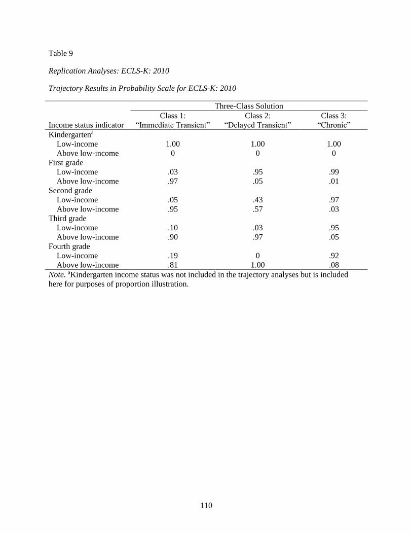
110

Table 9




Three-Class Solution

Class 1:

“Immediate Transient”

Class 2:

“Delayed Transient”

Class 3:

“Chronic”

Kindergartena

Low-income 1.00 1.00 1.00

Above low-income 0 0 0

First grade

Low-income .03 .95 .99

Above low-income .97 .05 .01

Second grade



Third grade



Fourth grade

Low-income .19 0 .92

Above low-income .81 1.00 .08

Note. aKindergarten income status was not included in the trajectory analyses but is included

here for purposes of proportion illustration.

111

Table 10


Descriptives of ECLS-K: 2010 Trajectories at Kindergarten

Proportion or Mean

Class 1:


Class 2:


Class 3:

“Chronic”


Age in years M(SD) 35.47 (5.27) 36.60 (4.87) 35.76 (6.30)

% White 73.1 66.7 52.0

% Black 7.1 11.1 10.5

% Hispanica 7.1 16.7 21.6

% Other race/ethnicity 12.5 5.6 15.9

% Married 77.2 85.5 78.6

% Mother has highest degree 63.2 65.5 56.1

% Father has highest degree 26.3 23.6 29.4

% Parents have equal degrees 10.5 10.9 14.5

% Working full-time 59.6 55.1 46.2

% Working part-time 25.5 18.4 24.2

% Other parent working full/part-time 81.6 88.0 66.0

Income in dollars M(SD) 37,482.49 (12,000.72) 36,760.05 (12,787.39) 30,972.12 (14,386.01)

Household size M(SD) 4.60 (1.22) 4.64 (1.14) 5.10 (1.63)

Warmth toward child M (SD) 3.68 (.29) 3.66 (.31) 3.68 (.33)


% High school diploma 0 2.0 3.2

% 4- or 5-year college degree 61.7 61.2 51.4

% Post-graduate degree 29.8 30.6 37.4


Age in years M(SD) 6.23 (.35) 6.16 (.32) 6.10 (.37)

% White 68.4 60.0 46.6

% Black 5.3 9.1 10.4

% Hispanica 12.3 16.4 24.9

% Other race/ethnicity 14.1 14.6 18.2

% Female 54.4 41.8 51.0


Reading IRT scores M(SD) 72.72 (14.73) 71.89 (13.21) 68.06 (14.13)

Math IRT scores M(SD) 56.60 (12.47) 53.13 (9.91) 49.61 (12.25)

Note. aHispanic includes “Hispanic, race specified” and “Hispanic, race not specified”

112

Table 11



aClass 2: “Delayed Transient” Class 3: “Chronic”

Predictor Estimate

B

SE Odds Ratio

e(B)

Estimate

B

SE Odds Ratio

e(B)

Father higher-educated (vs. Mother higher-educated) -1.17 .75 .31 .09 .56 1.09

Equally-educated parents (vs. Mother higher-educated) -.80 .87 .45 -.35 .60 .70

Parent identifies as Black (vs. parent identifies as White) .94 1.35 2.56 .72 .86 2.05

Parent identifies as Hispanic (vs. parent identifies as White) 1.39 1.23 4.01 1.54 1.01 4.66



-.77 1.11 .46 .34 .65 1.40

Parent married (vs. not married) 2.06 1.35 7.85 .08 .55 1.08

Parent working full-time (vs. not working) 1.14 .98 3.13 .38 .76 1.46

Parent working part-time (vs. not working) .41 .94 1.51 .15 .70 1.16

Parent with teaching occupation (vs. other occupation) -.29 .99 .75 -.40 .79 .67

Parent with service occupation (vs. other occupation) -1.93 1.25 .15 -.37 .69 .69



-1.30 .94 .27 -.81 .67 .44

Income at or below 100% of poverty threshold

(vs. above 100%)

.67 .91 1.95 1.35 .69 3.86

City locale (vs. Suburb locale) .16 .75 1.17 .32 .52 1.38

Rural locale (vs. Suburb locale) .47 .75 1.60 .21 .51 1.23

Note. aClass 1: “Immediate Transient” served as the reference group. bParent with occupation requiring a postsecondary degree refers to

occupations other than teaching and service. The Holm-Bonferonni correction method adjusted the p-value to account for multiple

comparisons. The R3STEP command in Mplus uses listwise deletion for missing data. *** p < .001, ** p < .01, * p < .05

113

Table 12



Class 1:


Class 2:


Class 3:

“Chronic” Overall

Chi-square Distal outcome Residual Mean SE Residual Mean SE Residual Mean SE

Parental education expectations .24 .12 .32 .14 .15 .07 1.34

Parental school involvement -.33 .27 .02 .16 .01 .06 1.50

Parental school satisfaction .13 .13 -.07 .10 -.11 .06 3.52

Parental rules -.43 .09 .19 .02 .21 .01 48.24***a, b

Parental warmth -.06 .07 -.05 .07 .03 .02 2.85

Parent-child education interactions -.22 .20 .20 .13 -.06 .08 4.11

Parent-child activities -.09 .53 -.26 .51 .53 .24 2.72

Children’s reading IRT scores .91 1.44 .43 1.07 .11 .68 .27

Children’s math IRT scores -2.03 1.38 .54 1.33 .17 .88 2.16

Note. aClass 1 significantly differs from Class 2, p < .001, bClass 1 significantly differs from Class 3, p < .001. Residuals calculated from a linear

regression with the following baseline predictors: parental marital status, parent working status, parental educational expectations, parental

warmth, child sex, child race, and child age. The Holm-Bonferonni correction method adjusted the p-value to account for multiple comparisons.

*** p < .001, ** p < .01, * p < .05

114

Table 13

Post hoc analyses: Descriptives

Means and Standard Deviations of Distal Outcomes by Income and Education Family Types in the ECLS-K: 1998

Distal outcomes

Low-income/High-education

M(SD)

Low-income/

Low-education

M (SD)

High-income/

Low-education

M (SD)

High-income/

High-education

M (SD) “Transient” “Chronic”

Parental education expectations 4.47 (.93) 4.12 (1.06) 3.83 (1.25) 3.95 (.97) 4.46 (.83)

Parental school involvement 3.24 (1.62) 2.61 (1.68) 2.12 (1.67) 2.57 (1.65) 3.01 (1.61)

Parental school satisfaction 9.00 (1.07) 8.82 (1.27) 8.62 (1.26) 8.95 (1.15) 9.23 (.99)

Parental rules 5.21 (1.80) 5.04 (1.87) 5.34 (1.80) 5.13 (1.68) 5.13 (1.70)

Parental warmth 7.55 (3.55) 6.51 (3.80) 6.54 (3.67) 7.31 (3.92) 7.40 (4.19)

Parent-child education interactions 7.26 (1.18) 7.23 (1.08) 7.43 (.95) 7.45 (.91) 7.30 (.97)

Parent-child activities 24.11 (3.12) 23.28 (3.41) 22.09 (3.80) 23.84 (2.89) 24.42 (2.48)

Children’s reading IRT scores 181.58 (22.98) 173.05 (25.18) 156.36 (29.22) 172.63 (23.91) 185.62 (19.12)

Children’s math IRT scores 152.27 (16.68) 145.13 (21.45) 131.35 (23.49) 142.92 (19.35) 153.20 (15.94)

Note. Descriptives are only for available data.

115

Table 14

Post hoc analyses: Descriptives

Means and Standard Deviations of Distal Outcomes by Income and Education Family Types in the ECLS-K: 2010

Distal outcomes

Low-income/High-education M(SD) Low-income/

Low-education

M (SD)

High-income/

Low-education

M (SD)

High-income/

High-education

M (SD) “Immediate

Transient”

“Delayed

Transient” “Chronic”

Parental education expectations 5.36 (.94) 5.44 (.92) 5.40 (1.15) 5.04 (1.48) 4.90 (1.23) 5.42 (.90)

Parental school involvement 3.54 (1.38) 3.84 (.96) 3.62 (1.05) 3.22 (1.24) 3.55 (1.14) 4.00 (.96)

Parental school satisfaction 3.79 (.41) 3.62 (.49) 3.62 (.66) 3.61 (.66) 3.65 (.61) 3.72 (.54)

Parental rules 1.81 (.53) 1.84 (.42) 1.83 (.45) 1.69 (.62) 1.76 (.51) 1.81 (.45)

Parental warmth 3.68 (.34) 3.61 (.39) 3.67 (.38) 3.61 (.41) 3.66 (.36) 3.69 (.34)

Parent-child education interactions 3.40 (1.10) 3.55 (.74) 3.48 (.96) 3.54 (1.02) 3.52 (.95) 3.45 (.96)

Parent-child activities 13.69 (3.08) 13.67 (2.83) 14.40 (3.35) 14.09 (3.34) 13.99 (3.03) 13.77 (2.75)

Children’s reading IRT scores 128.40 (9.34) 127.17 (9.14) 123.00 (12.98) 116.79 (14.75) 123.05 (11.17) 128.63 (10.04)

Children’s math IRT scores 116.89 (11.07) 115.33 (9.37) 110.63 (16.72) 103.33 (16.27) 110.40 (13.70) 116.77 (12.24)

Note. Descriptives are only for available data.

116

Table 15

Sensitivity Analyses: Dataset Differences

Fit Indices for ECLS-K: 1998 Income Status Trajectory Classes (n = 537)

Fit indices 1 class 2 class 3 class 4 classa

AIC 1755.12 1546.53 1550.61 1556.55

BIC 1763.69 1567.96 1584.89 1603.70

BIC adjusted 1757.34 1552.09 1559.50 1568.78

Entropy n/a .71 .82 .66

Vuong-Lo-Mendell-Rubin LRT n/a p < .001 p = .349 p < .001

Class 1 % 100 .70 74.83 67.99

Class 2 % .30 20.37 16.35

Class 3 % 4.80 15.67

Class 4 % 0

Note. aClass 4 had convergence issues, which is often indicative of poor model fit due to over

extraction of classes. Parametric likelihood ratio bootstrap test (BLRT; TECH14) cannot be

used with survey weights. All values were rounded to the nearest hundredth.

117

Table 16




Two-Class Solution


Kindergartena



First grade

Low-income .30 .93


Third grade

Low-income .20 .90


Fifth grade

Low-income .13 .85




118

Table 17


Fit Indices for ECLS-K: 2011 Income Status Trajectory Classes (n = 417)


AIC 1101.21 850.96 852.24 858.24

BIC 1109.28 871.13 884.50 902.60

BIC adjusted 1102.93 855.26 859.12 867.70

Entropy n/a .91 .96 .93


Class 1 % 100 81.78 80.41 80.41

Class 2 % 18.22 17.48 17.48

Class 3 % 2.12 2.12

Class 4 % 0



119

Table 18




Two-Class Solution


Kindergartena



First grade

Low-income .59 .98


Third grade

Low-income .09 .96


Fourth grade

Low-income .03 .94




120

Table 19





Father higher-educated (vs. Mother higher-educated) 1.15 .72 3.16

Equally-educated parents (vs. Mother higher-educated) -1.57 .75 .21

Parent identifies as Black (vs. parent identifies as White) 1.13 .66 3.10




.97 1.19 2.64


Parent working full-time (vs. not working) .70 .86 2.01

Parent working part-time (vs. not working) 1.25 1.13 3.49


Parent with service occupation (vs. other occupation) 2.35 1.71 10.49



-1.56 .55 .21 **

Income 101-150% of poverty threshold (vs. 151-200%) 2.00 1.05 7.39


Income 0-50% of poverty threshold (vs. 151-200%) -1.60 .79 .20

City locale (vs. Suburb locale) 1.30 .69 3.67


Note. aClass 1: “Transient” served as the reference group. bParent with occupation requiring a postsecondary

degree refers to occupations other than teaching and service. The Holm-Bonferonni correction method adjusted

the p-value to account for multiple comparisons. The R3STEP command in Mplus uses listwise deletion for

missing data. *** p < .001, ** p < .01, * p < .05

121

Table 20






Equally-educated parents (vs. Mother higher-educated) .31 .53 1.36

Parent identifies as Black (vs. parent identifies as White) .85 .73 2.34




.71 .68 2.03

Parent married (vs. not married) -.41 .48 .66

Parent working full-time (vs. not working) -.59 .57 .55

Parent working part-time (vs. not working) -.29 .53 .75


Parent with service occupation (vs. other occupation) -.08 .57 .92



-.21 .52 .81


(vs. above 100%)

.60 .51 1.82


Rural locale (vs. Suburb locale) -.14 .42 .87

Note. aClass 1: “Transient” served as the reference group. bParent with occupation requiring a postsecondary

degree refers to occupations other than teaching and service. The Holm-Bonferonni correction method adjusted

the p-value to account for multiple comparisons. The R3STEP command in Mplus 7.0 uses listwise deletion for

missing data. *** p < .001, ** p < .01, * p < .05

122

Table 21





Parental education expectations .30 .10 -.17 .06 13.02***

Parental school involvement 2.50 .24 -.15 .12 1.54

Parental school satisfaction .40 .45 -.23 .21 1.00

Parental rules -.20 .18 .13 .11 1.69

Parental warmth -.01 .05 -.01 .03 .02

Parent-child education interactions .09 .26 -.02 .15 .11

Parent-child activities .07 .11 -.04 .07 .69

Children’s reading IRT scores 3.46 2.70 -2.31 1.77 2.59

Children’s math IRT scores 2.71 1.88 -2.50 1.67 3.65

Note. Residuals calculated from a linear regression with the following baseline predictors: parental marital status,

parent working status, parental educational expectations, parental warmth, child sex, child race, and child age.

The Holm-Bonferonni correction method adjusted the p-value to account for multiple comparisons.

*** p < .001, ** p < .01, * p < .05

123

Table 22


Differences in Distal Outcome Means between Trajectory Classes in ECLS-K: 2011 (N =417)



Parental education expectations .37 .11 .15 .06 3.14

Parental school involvement .04 .13 -.05 .07 .33

Parental school satisfaction -.01 .07 -.10 .05 .92

Parental rules -.25 .07 .21 .01 37.15***

Parental warmth .00 .04 .01 .02 .03

Parent-child education interactions .01 .13 -.05 .07 .16

Parent-child activities .05 .40 .43 .23 .64

Children’s reading IRT scores 1.00 1.01 .14 .66 .49

Children’s math IRT scores -.27 1.12 -.14 .84 .93

Note. Residuals calculated from a linear regression with the following baseline predictors: parental marital

status, parent working status, parental educational expectations, parental warmth, child sex, child race, and child

age. The Holm-Bonferonni correction method adjusted the p-value to account for multiple comparisons.

*** p < .001, ** p < .01, * p < .05

124

Table 23

Sensitivity Analyses: Data Collection Intervals



AIC 1500.48 1066.20 1043.93 1042.63

BIC 1508.69 1086.73 1076.79 1087.80

BIC adjusted 1502.34 1070.87 1051.40 1052.89

Entropy n/a .92 .96 .93


Class 1 % 100 80.70 80.70 80.70

Class 2 % 19.30 10.70 13.03

Class 3 % 8.61 4.36

Class 4 % 1.91



125

Table 24

Sensitivity Analyses: Data Collection Intervals



Three-Class Solution

Class 1:


Class 2:


Class 3:

“Chronic”

Kindergartena

Low-income 1.00 1.00 1.00

Above low-income 0 0 0

First grade

Low-income .04 1.00 .99

Above low-income .96 0 .01

Second grade



Third grade



Fourth grade



Note. aKindergarten income status was not included in the trajectory analyses but is included

here for purposes of proportion illustration.

126

Table 25

Sensitivity Analyses: Multiple Imputation

Sociodemographic Predictors of Income Status Trajectory Membership in ECLS-K: 1998 (N = 540)




Equally-educated parents (vs. Mother higher-educated) -.77 .45 .46

Parent identifies as Black (vs. parent identifies as White) 1.15 .50 3.16




.67 .45 1.95


Parent working full-time (vs. not working) -1.81 1.51 .16

Parent working part-time (vs. not working) -1.56 1.64 .21


Parent with service occupation (vs. other occupation) 1.60 .78 4.95



-.05 1.59 .95

Income 0-50% of poverty threshold (vs. 151-200%) -.68 .46 .51





Note. aClass 1: “Transient” served as the reference group. bParent with occupation requiring a postsecondary degree

refers to occupations other than teaching and service. The Holm-Bonferonni correction method adjusted the p-value

to account for multiple comparisons. The R3STEP command in Mplus 7.0 uses listwise deletion for missing data.

*** p < .001, ** p < .01, * p < .05

127

Table 26

Sensitivity Analyses: Multiple Imputation

Sociodemographic Predictors of Income Status Trajectory Membership in ECLS-K: 2010 (N = 449)

aClass 2: “Delayed Transient” Class 3: “Chronic”

Predictor Estimate

B

SE Odds Ratio

e(B)

Estimate

B

SE Odds Ratio

e(B)

Father higher-educated (vs. Mother higher-educated) -.76 .68 .47 .22 .48 1.25

Equally-educated parents (vs. Mother higher-educated) -.29 .82 .75 .28 .58 1.32

Parent identifies as Black (vs. parent identifies as White) .93 .97 2.53 1.08 .69 2.94

Parent identifies as Hispanic (vs. parent identifies as White) 1.42 1.01 4.14 1.47 .79 4.35


(v. parent identifies as White)

-.75 .95 .47 .36 .55 1.43

Parent married (vs. not married) 1.19 .83 3.29 .30 .43 1.35

Parent working full-time (vs. not working) .78 1.07 2.18 .33 .78 1.39

Parent working part-time (vs. not working) .33 1.14 1.39 .29 .81 1.34

Parent with teaching occupation (vs. other occupation) .36 .68 1.43 .10 .54 1.11

Parent with service occupation (vs. other occupation) -1.45 1.23 .23 .07 .58 1.07



.01 1.17 1.01 -.51 .84 .60


(vs. above 100%)

1.18 .80 3.25 1.60 .61 4.95 **

City locale (vs. Suburb locale) -.28 .64 .76 -.33 .44 .72

Rural locale (vs. Suburb locale) .09 .62 1.09 -.06 .47 .94

Note. aClass 1: “Immediate Transient” served as the reference group. bParent with occupation requiring a postsecondary degree refers to

occupations other than teaching and service. The Holm-Bonferonni correction method adjusted the p-value to account for multiple

comparisons. The R3STEP command in Mplus uses listwise deletion for missing data. *** p < .001, ** p < .01, * p < .05

128

Figure 1. Original analyses: ECLS-K: 1998 income status trajectories over time

129

Figure 2. Replication analyses: ECLS-K: 2010 income status trajectories over time

130

Figure 3. Sensitivity analyses for dataset differences: ECLS-K: 1998 income status trajectories over time

131

Figure 4. Sensitivity analyses for dataset differences: ECLS-K: 2010 income status trajectories over time

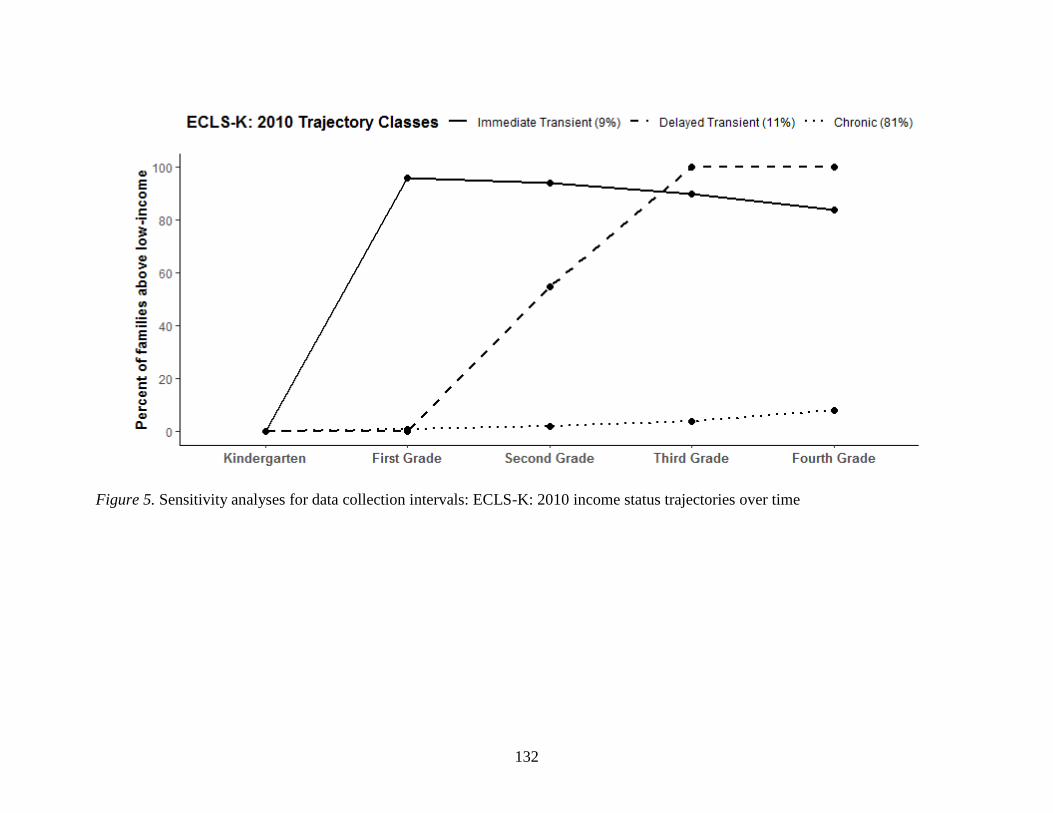
132

Figure 5. Sensitivity analyses for data collection intervals: ECLS-K: 2010 income status trajectories over time

133

APPENDICES

134

APPENDIX A

Income category codes in ECLS-K: 1998

1 = $5,000 or less

2 = $5,001 to $10,000

3 = $10,001 to $15,000

4 = $15,001 to $20,000

5 = $20,001 to $25,000

6 = $25,001 to $30,000

7 = $30,001 to $35,000

8 = $35,001 to $40,000

9 = $40,001 to $50,000

10 = $50,001 to $75,000

11 = $75,001 to $100,000

12 = $100,001 to $200,000

13 = $200,001 or more

135

APPENDIX B

Income category codes in ECLS-K: 2011

1 = $5,000 or less

2 = $5,001 to $10,000

3 = $10,001 to $15,000

4 = $15,001 to $20,000

5 = $20,001 to $25,000

6 = $25,001 to $30,000

7 = $30,001 to $35,000

8 = $35,001 to $40,000

9 = $40,001 to $45,000

10 = $45,001 to $50,000

11 = $50,001 to $55,000

12 = $55,001 to $60,000

13 = $60,001 to $65,000

14 = $65,001 to $70,000

15 = $70,001 to $75,000

16 = $75,001 to $100,000

17 = $100,001 to $200,000

18 = $200,001 or more

136

APPENDIX C

Low-income thresholds for ECLS-K: 1998

The income variable asks participants for their previous year’s income. Therefore, thresholds

correspond to the previous year, not the date of data collection.

Table 27

Thresholds for 1998 (Wave 2, Kindergarten)

Household

total

Poverty

threshold

200% poverty

threshold

2 $10,972 $21,944

3 $13,003 $26,006

4 $16,660 $33,320

5 $19,680 $39,360

6 $22,228 $44,456

7 $25,257 $50,514

8 $28,166 $56,332

9+ $33,339 $66,678

Table 28

Thresholds for 1999 (Wave 4, First Grade)

Household

total

Poverty

threshold

200% poverty

threshold

ECLS-K income

category

ECLS-K income

category value

2 $11,214 $22,428 $20,001 to $25,000 5

3 $13,290 $26,580 $25,001 to $30,000 6

4 $17,029 $34,058 $30,001 to $35,000 7

5 $20,127 $40,254 $35,001 to $40,000 8

6 $22,727 $45,454 $40,001 to $50,000 9

7 $25,912 $51,824 $50,001 to $75,000 10

8 $28,967 $57,934 $50,001 to $75,000 10

9+ $34,417 $68,834 $50,001 to $75,000 10

137

Table 29

Thresholds for 2001 (Wave 5, Third Grade)

Household

total

Poverty

threshold

200% poverty

threshold

ECLS-K income

category

ECLS-K income

category value

2 $11,920 $23,840 $20,001 to $25,000 5

3 $14,128 $28,256 $25,001 to $30,000 6

4 $18,104 $36,208 $35,001 to $40,000 8

5 $21,405 $42,810 $40,001 to $50,000 9

6 $24,195 $48,390 $40,001 to $50,000 9

7 $27,517 $55,034 $50,001 to $75,000 10

8 $30,627 $61,254 $50,001 to $75,000 10

9+ $36,286 $72,572 $50,001 to $75,000 10

Table 30

Thresholds for 2003 (Wave 6, Fifth Grade)

Household

total

Poverty

threshold

200% poverty

threshold

ECLS-K income

category

ECLS-K income

category value

2 $12,384 $24,768 $20,001 to $25,000 5

3 $14,680 $29,360 $25,001 to $30,000 6

4 $18,810 $37,620 $35,001 to $40,000 8

5 $22,245 $44,490 $40,001 to $50,000 9

6 $25,122 $50,244 $50,001 to $75,000 10

7 $28,544 $57,088 $50,001 to $75,000 10

8 $31,589 $63,178 $50,001 to $75,000 10

9+ $37,656 $75,312 $75,001 to $100,000 11

Table 31

Thresholds for 2006 (Wave 7, Eighth Grade)

Household

total

Poverty

threshold

200% poverty

threshold

ECLS-K income

category

ECLS-K income

category value

2 $13,569 $27,138 $25,001 to $30,000 6

3 $16,079 $32,158 $30,001 to $35,000 7

4 $20,614 $41,228 $40,001 to $50,000 9

5 $24,382 $48,764 $40,001 to $50,000 9

6 $27,560 $55,120 $50,001 to $75,000 10

7 $31,205 $62,410 $50,001 to $75,000 10

8 $34,774 $69,548 $50,001 to $75,000 10

9+ $41,499 $82,998 $75,001 to $100,000 11

138

APPENDIX D

Low-income thresholds for ECLS-K: 2010

The income variable asks participants for their previous year’s income. Therefore, thresholds

correspond to the previous year, not the date of data collection.

Table 32

Thresholds for 2010 (Wave 2, Kindergarten)

Household

total

Poverty

threshold

200% poverty

threshold

2 $14,676 $29,352

3 $17,374 $34,748

4 $22,314 $44,628

5 $26,439 $52,878

6 $29,897 $59,794

7 $34,009 $68,018

8 $37,934 $75,868

9+ $45,220 $90,440

Table 33

Thresholds for 2011 (Wave 4, First Grade)

Household

total

Poverty

threshold

200% poverty

threshold

ECLS-K income

category

ECLS-K income

category value

2 $15,139 $30,278 $25,001 to $30,000 6

3 $17,916 $35,832 $35,001 to $40,000 7

4 $23,021 $46,042 $45,001 to $50,000 10

5 $27,251 $54,502 $50,001 to $55,000 11

6 $30,847 $61,694 $60,001 to $65,000 13

7 $35,085 $70,170 $65,001 to $70,000 14

8 $39,064 $78,128 $75,001 to $100,000 16

9+ $46,572 $93,144 $75,001 to $100,000 16

139

Table 34

Thresholds for 2012 (Wave 6, Second Grade)

Household

total

Poverty

threshold

200% poverty

threshold

ECLS-K income

category

ECLS-K income

category value

2 $15,450 $30,900 $25,001 to $30,000 6

3 $18,284 $36,568 $35,001 to $40,000 8

4 $23,492 $46,984 $45,001 to $50,000 10

5 $27,827 $55,654 $50,001 to $55,000 11

6 $31,471 $62,942 $60,001 to $65,000 13

7 $35,743 $71,486 $70,001 to $75,000 15

8 $39,688 $79,376 $75,001 to $100,000 16

9+ $47,297 $94,594 $75,001 to $100,000 16

Table 35

Thresholds for 2013 (Wave 7, Third Grade)

Household

total

Poverty

threshold

200% poverty

threshold

ECLS-K income

category

ECLS-K income

category value

2 $15,679 $31,358 $30,001 to $35,000 7

3 $18,552 $37,104 $35,001 to $40,000 8

4 $23,834 $47,668 $45,001 to $50,000 10

5 $28,265 $56,530 $55,001 to $60,000 12

6 $31,925 $63,850 $60,001 to $65,000 13

7 $36,384 $72,768 $70,001 to $75,000 15

8 $40,484 $80,968 $75,001 to $100,000 16

9+ $48,065 $96,130 $75,001 to $100,000 16

Table 36

Thresholds for 2014 (Wave 8, Fourth Grade)

Household

total

Poverty

threshold

200% poverty

threshold

ECLS-K income

category

ECLS-K income

category value

2 $15,934 $31,868 $30,001 to $35,000 7

3 $18,850 $37,700 $35,001 to $40,000 8

4 $24,230 $48,460 $45,001 to $50,000 10

5 $28,695 $57,390 $55,001 to $60,000 12

6 $32,473 $64,946 $60,001 to $65,000 13

7 $36,927 $73,854 $70,001 to $75,000 15

8 $40,968 $81,936 $75,001 to $100,000 16

9+ $49,021 $98,042 $75,001 to $100,000 16

140

Table 37

Thresholds for 2015 (Wave 9, Fifth Grade)

Household

total

Poverty

threshold

200% poverty

threshold

ECLS-K income

category

ECLS-K income

category value

2 $15,952 $31,904 $30,001 to $35,000 7

3 $18,871 $37,742 $35,001 to $40,000 8

4 $24,257 $48,514 $45,001 to $50,000 10

5 $28,741 $57,482 $55,001 to $60,000 12

6 $32,542 $65,084 $60,001 to $65,000 13

7 $36,998 $73,996 $70,001 to $75,000 15

8 $41,029 $82,058 $75,001 to $100,000 16

9+ $49,177 $98,354 $75,001 to $100,000 16

141

APPENDIX E

Parent occupation codes for ECLS-K: 1998 and ECLS-K: 2010

1 = Executive, Administrative, and Managerial Occupations

2 = Engineers, Surveyors, and Architects

3 = Natural Scientists and Mathematicians

4 = Social Scientists, Social Workers, Religious Workers, and Lawyers

5 = Postsecondary Institution Teachers, Counselors, Librarians, Archivists

6 = Teachers, except Postsecondary Institutions

7 = Health Diagnosing and Treating Practitioners

8 = Registered Nurses, Pharmacists, Dieticians, Therapists, and Physician’s Assistants

9 = Writers, Artists, Entertainers, and Athletes

10 = Health Technologists and Technicians

11 = Technologists and Technicians, except Health

12 = Marketing and Sales Occupations

13 = Administrative Support Occupations, including Clerical

14 = Service Occupations

15 = Agriculture, Forestry, and Fishing Occupations

16 = Mechanics and Repairers

17 = Construction and Extractive Occupations

18 = Precision Production Occupations

19 = Production Working Occupation

142

20 = Transportation and Material Moving Occupations

21 = Handlers, Equipment Cleaners, Helpers, and Laborers

22 = Unemployed, Retired, Disabled, or Unclassified Workers

143

APPENDIX F

Fifth grade distal outcome measures for ECLS-K: 1998 sensitivity analyses

Distal outcome variables. The distal outcomes related to parent and child behavior were

collected in fifth grade of the ECLS-K: 1998 (Wave 7) unless otherwise noted.

Parental educational expectations. Parent educational expectations consisted of one item

that asked parents, “How far in school do you expect {child} to go?” (1 = receiving less than a

high school diploma to 6 = getting a Ph.D., M.D., or other high degree).

Parental school involvement. Parents were asked, “Since the beginning of this school

year, have you or the other adults in your household…”: attended an open house or back-to-

school night, attended a parent-teacher association or organization meeting, attended regularly

scheduled parent-teacher conferences, attended a school event, acting as a volunteer at school or

served on a committee, and participated in fundraising. Items were dichotomously coded (0 = no,

1 = yes). These six items were then summed, with higher scores representing more parental

school involvement.

Parental school satisfaction. At third grade (Wave 6), parents were asked how well their

child’s school has done with each of the following activities during this school year: school lets

parent know between report cards how child is doing in school, school helps parent understand

what children at that age are like, school makes parent aware of chances to volunteer at school,

and school provides workshops, materials, or advice about how to help child learn at home.

Items were rated on a 3-point scale (1 = does this very well, 2 = just ok, 3 = does not do this at

144

all). Items were reverse coded for analyses and summed so that higher values indicated more

satisfaction with the school.

Parental rules. Parents were asked, “Are there family rules for {child} about any of the

following…”: which television programs the child can watch, how early or late the child may

watch television, the number of hours of television the child can watch on weekdays, and the

number of hours the child can watch television each week. Items were dichotomously coded (0 =

no, 1 = yes). These four items were then summed, with higher scores representing more family

rules.

Parental warmth. At third grade (Wave 6), parents rated six items such as “{Child} and I

often have warm, close times together” and “Even when I’m in a bad mood, I show {child} a lot

of love”. Items were rated on a 4-point scale (1 = completely true, 2 = mostly true, 3 = somewhat

true, 4 = not at all true). Items were reverse coded for analyses so that higher values indicated

greater warmth. These six items were then averaged (α = .67).

Parent-child education interactions. Parents were asked how often someone helped their

child with reading, language arts, or spelling homework and homework in math. Items were

dichotomously coded (0 = no, 1 = yes). These two items were then summed, with higher scores

representing higher frequency of parent-child education interactions.

Parent-child activities. At third grade (Wave 6), parents indicated if anyone in their

family had engaged in the following four activities with their child (0 = no, 1 = yes): visited the

library, gone to a play, concert, or other live show, visited an art gallery, museum, or historical

site, and visited a zoo, aquarium, or petting farm. These five items were then summed, with

higher scores representing more parent-child activities.

145

Child achievement. Achievement was measured by using Item Response Theory (IRT)

achievement scores in reading and math. IRT procedures use correct and incorrect responses to

tailor testing to a child’s individual academic ability at each grade level. IRT can estimate the

probability of correct responses for all questions by using the child’s pattern of responses. The

IRT achievement scores in reading and math available in the ECLS-K have been shown to be

reliable within and across time (Pollack, Atkins-Burnett, Rock, & Weiss, 2005). Reading and

math achievement measures were examined individually.

146

REFERENCES

147

Abdi, H. (2010). Holm’s sequential Bonferroni procedure. In N. Salkind (Ed.), Encyclopedia of

research design (pp. 574-578). Thousand Oaks, CA: Sage.

Aber, J. L., Bennett, N. G., Conley, D. C., & Li, J. (1997). The effects of poverty on child health

and development. Annual Review of Public Health, 18(1), 463-483.

Aikens, N. L., & Barbarin, O. (2008). Socioeconomic differences in reading trajectories: The

contribution of family, neighborhood, and school contexts. Journal of Educational

Psychology, 100(2), 235-251.

Akee, B. R. K. Q., Copeland, W. E., Keeler, G., Angold, A., & Costello, E. J. (2010). Parents’

incomes and children’s outcomes: A quasi-experiment using transfer payments from

casino profits. American Economic Journal, 2(1), 86-115.

American Academy of Arts & Sciences. (2018). The state of the humanities 2018: Graduates in

the workforce and beyond. Cambridge, MA: American Academy of Arts & Sciences.

Retrieved from

http://www.amacad.org/sites/default/files/academy/multimedia/pdfs/publications/research

papersmonographs/HI_Workforce-2018.pdf

Anderson, E. (1999). Code of the street: Decency, violence, and the moral life of the inner city.

New York, NY: Norton.

Anderson, R. (2011). Dynamics of economic well-being: Poverty, 2004-2006. Current

Population Reports, Series P70-123. Washington, DC: U.S. Census Bureau. Retrieved

from https://www.census.gov/prod/2011pubs/p70-123.pdf

Andruff, H., Carraro, N., Thompson, A., Gaudreau, P., & Louvet, B. (2009). Latent class growth

modelling: A tutorial. Tutorials in Quantitative Methods for Psychology, 5(1), 11-24.

https://doi.org/10.20982/tqmp.05.1.p011

Asparouhov, T., & Muthén, B. (2010). Multiple imputation with Mplus. Mplus. Retrieved from

https://www.statmodel.com/download/Imputations7.pdf

Asparouhov, T., & Muthén, B. (2013). Auxiliary variables in mixture modeling : 3-Step

approaches using Mplus. Mplus Web Notes: No. 15. Retrieved from

http://statmodel.com/examples/webnotes/AuxMixture_submitted_corrected_webnote.pdf

Asparouhov, T., & Muthén, B. (2014). Auxiliary variables in mixture modeling: Three-step

approaches using Mplus. Structural Equation Modeling, 21(3), 329-341.

https://doi.org/10.1080/10705511.2014.915181.

Austin, P. C., & Steyerberg, E. W. (2017). Events per variable (EPV) and the relative

performance of different strategies for estimating the out-of-sample validity of logistic

regression models. Statistical Methods in Medical Research, 26(2), 796-808.

148

Babyak, M. A. (2004). What you see may not be what you get: A brief, nontechnical

introduction to overfitting in regression-type-models. Psychosomatic Medicine, 66, 411-

421.

Bane, M. J., & Ellwood, D. (1986). Slipping into and out of poverty: The dynamics of spells.

Journal of Human Resources, 21, 1-23.

Batlova, J., Fix, M., & Bachmeier, J. D. (2016). Untapped talent: The cost of brain waste among

highly skilled immigrants in the United States. Washington, DC: Migration Policy

Institute, New American Economy, and World Education Services. Retrieved from

https://www.migrationpolicy.org/research/untapped-talent-costs-brain-waste-among-

highly-skilled-immigrants-united-states

Bauer, D. J., & Curran, P. J. (2004). The integration of continuous and discrete latent variable

models: Potential problems and promising opportunities. Psychological Methods, 9(1), 3-

29.

Becker, G. S. (1991). A treatise on the family. Cambridge, MA: Cambridge University Press.

Becker, G. S., & Tomes, N. (1986). Human capital and the rise and fall of families. Journal of

Labor Economics, 4(3), S1-S39.

Becker, G. S., & Tomes, N. (1994). Human capital: A theoretical and empirical analysis with

special reference to education (3rd ed.). Chicago, IL: University of Chicago Press.

Belsky, J. (1998) Paternal influence and children’s well being: limits of and new directions for

understanding. In A. Booth (Ed.), Men in families: When do they get involved? What

differences does it make? Mahwah,NJ: Lawrence Erlbaum Associates.

Bennett, D. A. (2001). How can I deal with missing data in my study?. Australian and New

Zealand Journal of Public Health, 25(5), 464-469.

Berger, L. M., Cancian, M., & Magnuson, K. (2018). Anti-poverty policy innovations : New

proposals for addressing poverty in the United States. The Russell Sage Foundation

Journal of Social Sciences, 4(3), 1-19. https://doi.org/10.7758/RSF.2018.4.3.01.

Bernstein, J., Brocht, C., & Spade-Aguilar, M. (2000). How much is enough? Basic family

budgets for working families. Washington, DC: Economic Policy Institute. Retrieved

from https://www.epi.org/files/page/-/old/books/HowMuchIsEnough_execsum.pdf

Bishaw, A. (2012). Poverty: 2010 and 2011. American Community Survey Briefs. Washington,

DC: United States Census Bureau. Retrieved from

https://www.census.gov/library/publications/2012/acs/acsbr11-01.html

Bourgois, P. (2001). Culture of poverty. In N. Smelser & P. Baltes (Eds.), International

encyclopedia of the social & behavioral sciences (pp. 11904-11907). Oxford, UK:

Pergamon.

149

Bower, C. (2013). Social policy and the achievement gap: What do we know? Where should we

head? Education and Urban Society, 45(1), 3-36.

Bradley, R. H., & Corwyn, R. F. (2002). Socioeconomic status and child development. Annual

Review of Psychology, 53, 371-99.

https://doi.org/10.1146annurev.psch.53.100901.135233

Bradley, R. H., Caldwell, Β., Rock, S., Ramey, C., Barnard, Κ. E., . . . Johnson, D. L. (1989).

Home environment and cognitive development in the first 3 years of life: A collaborative

study involving six sites. Developmental Psychology, 25(2), 217-235.

Brière, F. N., Rohde, P., Stice, E., & Morizot, J. (2016). Group-based symptom trajectories in

indicated prevention of adolescent depression. Depression and Anxiety, 33(5), 444-451.

https://doi.org/10.1002/da.22440

Brody, G. H., & Flor, D. L. (1997). Maternal psychological functioning, family processes, and

child adjustment in rural, single-parent, African American families. Developmental

Psychology, 33, 1000-1011.

Bronfenbrenner, U., & Morris, P. A. (2006). The bioecological model of human development. In

R. Lerner (Ed.), Handbook of child psychology (6th ed., pp. 793-828). New York, NY:

Wiley.

Brooks-Gunn, J., & Duncan, G. J. (1997). The effects of poverty on children. Children and

Poverty, 7(2), 55-71.

Button, K. S., Ioannidis, J. P., Mokrysz, C., Nosek, B. A., Flint, J., Robinson, E. S., & Munafò,

M. R. (2013). Power failure: Why small sample size undermines the reliability of

neuroscience. Nature Reviews Neuroscience, 14(5), 1-12.

Camarota, S. A., & Zeigler, K. (2018). Better educated, but not better off: A look at the

education level and socioeconomic success of recent immigrants, 2007 to 2017.

Washington, DC: Center for Immigration Studies. Retrieved from

https://cis.org/sites/default/files/2018-04/camarota-education.pdf

Campbell, D. (1986). Science’s social system of validity-enhancing collective belief change and

the problems of the social sciences. In D. Fiske & R. Shweder (Eds.), Metatheory in

social science (pp. 108-135). Chicago, IL: University of Chicago Press

Cellini, S. R., McKernan, S. M., & Ratcliffe, C. (2008). The dynamics of poverty in the United

States: A review of data, methods, and findings. Journal of Policy Analysis and

Management, 27(3), 577-605.

Center on Budget and Policy Priorities. (2019). Chart book: The legacy of the Great Recession.

Center on Budget and Policy Priorities. Retrieved from

https://www.cbpp.org/research/economy/chart-book-the-legacy-of-the-great-recession

150

Chase-Lansdale, P. L., & Brooks-Gunn, J. (2014). Two-generation programs in the 21st century.

Future of Children, 24(1), 13-39.

Chen, F., Carolina, N., Curran, P. J., Bollen, K. A, & Kirby, J. (2008). An empirical evaluation

of the use of fixed cutoff points in RMSEA test statistic in structural equation models.

Social Methods Research, 36(4), 1-31. https://doi.org/10.1177/0049124108314720.

Chetty, R., Hendren, N., Jones, M. R., & Porter, S. R. (2018). Race and economic opportunity in

the United States: An intergenerational perspective. NBER Working Paper Series, 24441.

Retrieved from https://www.nber.org/papers/w24441.pdf

Chetty, R., Hendren, N., Kline, P., Saez, E., & Turner, N. (2014). Is the United States still a land

of opportunity? Recent trends in intergenerational mobility. American Economic Review,

104(5), 141-47.

Citro, C., & Michael, R. (1995). Measuring poverty: A new approach. Washington, DC:

National Academy Press.

Cohen, J. (1988). Statistical power analysis for the behavioral sciences (2nd ed.). Hillsdale, NJ:

Cohn, D., Passell, J. S., Wang, W., & Livinston, G. (2011). Barely half of U.S. adults are

married – a record low. Washington, DC: Pew Research Center. Retrieved from

https://www.pewsocialtrends.org/2011/12/14/barely-half-of-u-s-adults-are-married-a-

record-low/

Collie, R. J., Shapka, J. D., Perry, N. E., & Martin, A. J. (2015). Teachers’ beliefs about social-

emotional learning: Identifying teacher profiles and their relations with job stress and

satisfaction. Learning and Instruction, 39, 148-157.

https://doi.org/10.1016/j.learninstruc.2015.06.002

Comer, J. P. (2005). The rewards of parent participation. Educational Leadership, 62(6), 38-42.

Conger, R. D., Conger, K. J., & Elder, G. H. (1997) Family economic hardship and adolescent

adjustment: Mediating and moderating processes. In G. J. Duncan & J. Brooks-Dunn

(Eds.), Consequences of growing up poor (pp. 288-310). New York, NY: Russell Sage

Foundation.

Conger, R. D., Conger, K. J., & Martin, M. J. (2010). Socioeconomic status, family processes,

and individual development. Journal of Marriage and Family, 72(3), 685-704.

Conger, R. D., Conger, K. J., Elder Jr, G. H., Lorenz, F. O., Simons, R. L., & Whitbeck, L. B.

(1992). A family process model of economic hardship and adjustment of early adolescent

boys. Child Development, 63(3), 526-541.

Conger, R. D., Ge, X., Elder Jr, G. H., Lorenz, F. O., & Simons, R. L. (1994). Economic stress,

coercive family process, and developmental problems of adolescents. Child Development,

65(2), 541-561.

151

Conger, R. D., Wallace, L. E., Sun, Y., Simons, R. L., McLoyd, V. C., & Brody, G. H. (2002).

Economic pressure in African American families: A replication and extension of the

family stress model. Developmental Psychology, 38(2), 179-193.

https://doi.org/10.1037/0012-1649.38.2.179

Cooper, D. (2017). Raising the minimum wage to $15 by 2024 would lift wages for 41 million

American workers. Washington, DC: Economic Policy Institute. Retrieved from

https://www.epi.org/files/pdf/125047.pdf

Corcoran, M. (1995). Rags to rags: Poverty and mobility in the United States. Annual Review of

Sociology, 21(1), 237-267.

Côté, S., House, J., & Willer, R. (2015). High economic inequality leads higher-income

individuals to be less generous. Proceedings of the National Academy of Sciences,

112(52), 15838-15843.

Cronbach, L. (1982). Designing evaluations of educational and social programs. San Francisco,

CA: Jossey-Bass.

Crosnoe, R., Purtell, K. M., Davis-Kean, P., Ansari, A., & Benner, A. D. (2016). The selection of

children from low-income families into preschool. Developmental Psychology, 52(4),

599-612.

Cunningham, E. (2018). Great Recession, great recovery? Trends from the Current Population

Survey. Monthly Labor Review, U. S. Bureau of Labor Statistics. Retrieved from

https://www.bls.gov/opub/mlr/2018/article/great-recession-great-recovery.htm

Curran, P. J., Obeidat, K., & Losardo, D. (2010). Twelve frequently asked questions about

growth curve modeling. Journal of Cognition and Development, 11(2), 121-136.

Dahl, B. G. B., & Lochner, L. (2018). The impact of family income on child achievement:

Evidence from the Earned Income Tax Credit. The American Economic Review, 102(5),

1927-1956.

Dalaker, J. (1999). Poverty in the United States: 1998. Current Population Reports, Series P60-

207. Washington, DC: United States Census Bureau. Retrieved from

https://www2.census.gov/library/publications/1999/demographics/p60-207.pdf

Davis-Kean, P. E. (2005). The influence of parent education and family income on child

achievement: The indirect role of parental expectations and the home environment.

Journal of Family Psychology, 19(2), 294-304. https://doi.org/10.1037/0893

3200.19.2.294

Davis-Kean, P. E., & Sexton, H. R. (2009). Race differences in parental influences on child

achievement. Merrill-Palmer Quarterly, 55(3), 285-318.

https://www.bls.gov/opub/mlr/2018/article/great-recession-great-recovery.htm

152

Davis-Kean, P. E., Jager, J., & Maslowsky, J. (2015). Answering developmental questions using

secondary data. Child Development Perspectives, 9(4), 256-261.

https://doi.org/10.1111/cdep.12151

Dearing, E. (2008). Psychological costs of growing up poor. Annals of the New York Academy of

Sciences, 1136, 324-332. https://doi.org/10.1196/annals.1425.006

Diemer, M. A., Mistry, R. S., Wadsworth, M. E., López, I., & Reimers, F. (2013). Best practices

in conceptualizing and measuring social class in psychological research. Analyses of

Social Issues and Public Policy, 13(1), 77-113. https://doi.org/10.1111/asap.12001

Diemer, M., & Mistry, R. (2018). Best practices in conceptualizing and measuring social class

with secondary data sources. Workshop presented at the Society for Research in Child

Development: Conference on the Use of Secondary and Open Source Data in

Developmental Science. Phoenix, AZ.

Donner, A. (1982). The relative effectiveness of procedures commonly used in multiple

regression analysis for dealing with missing values. The American Statistician, 36(4),

378-381.

Dubow, E. F., Boxer, P., & Huesmann, L. R. (2009). Long-term effects of parents’ education on

children’s educational and occupational success: Mediation by family interactions, child

aggression, and teenage aspirations. Merrill-Palmer Quarterly, 55(3), 224-249.

Duncan, G. J. (1984). Years of poverty--years of plenty: The changing economic fortunes of

American workers and families. Ann Arbor, MI: Institute for Social Research.

Duncan, G. J., & Magnuson, K. (2001). Off with Hollingshead: Socioeconomic resources,

parenting, and child development. In M. H. Bornstein & R. H. Bradley (Eds.),

Socioeconomic status, parenting, and child development (pp. 83-106). Mahwah, NJ:

Lawrence Erlbaum Associates.

Duncan, G. J., & Magnuson, K. (2005). Can family socio-economic resources account for test

score gain? Future of Children, 15(1), 15-34.

Duncan, G. J., & Magnuson, K. (2011). The nature and impact of early achievement skills,

attention and behavior problems. In G. J. Duncan & R. J. Murnane (Eds.), Whither

opportunity?: Rising inequality, schools, and children’s life chances (pp. 91-116). New

York, NY: The Russell Sage Foundation.

Duncan, G. J., & Magnuson, K. (2012). Socioeconomic status and cognitive functioning: moving

from correlation to causation. Cognitive Science, 3(3), 377-386.

Duncan, G. J., & Rodgers, W. L. (1988). Longitudinal aspects of childhood poverty. Journal of

Marriage and the Family, 50(4), 1007-1021. https://doi.org/10.2307/352111

153

Duncan, G. J., Engel, M., Claessens, A., & Dowsett, C. J. (2014). Replication and robustness in

developmental research. Developmental Psychology, 50(11), 2417-2425.

https://doi.org/10.1037/a0037996

Duncan, G. J., Huston, A. C., & Weisner, T. S. (2007). Higher ground: New hope for the

working poor and their children. New York, NY: Russell Sage Foundation.

Duncan, G. J., Kalil, A., & Ziol-Guest, K. M. (2017). Increasing inequality in parent incomes

and children’s schooling. Demography, 54, 1603-1626. https://doi.org/10.1007/s13524-

017-0600-4

Duncan, G. J., Magnuson, K., & Votruba-Drzal, E. (2017). Moving beyond correlations in

assessing the consequences of poverty. Annual Review of Psychology, 68, 413-434.

https://doi.org/10.1146/annurev-psych-010416-044224

Duncan, G. J., Morris, P. A., & Rodrigues, C. (2011). Does money really matter? Estimating

impacts of family income on young children's achievement with data from random-

assignment experiments. Developmental Psychology, 47(5), 1263-1279.

Duncan, G. J., Yeung, W. J., Brooks-Gunn, J., & Smith, J. R. (1998). How much does childhood

poverty affect the life chances of children? American Sociological Review, 63(3), 406-

423.

Duncan, G., Brooks-Gunn, J., & Klebanov, E (1994). Economic deprivation and early childhood

development. Child Development, 65, 296-318.

Dziak, J. J., Coffman, D. L., Lanza, S. T., Li, R., & Jermiin, L. S. (2012). Sensitivity and

specificity of information criteria. State College, PA: The Pennsylvania State University.

Retrieved from https://www.biorxiv.org/content/biorxiv/early/2019/01/08/449751.full.pdf

Eccles, J. S., & Harold, R. D. (1996). Family involvement in children’s and adolescents’

schooling. In A. Booth & J. F. Dunn (Eds.), Family-school links: How do they affect

educational outcomes (pp. 3-34). Mahwah, NJ: Lawrence Erlbaum Associates.

Edin, K., & Kefalas, M. (2005). Promises I can keep: Why poor women put motherhood before

marriage. Berkeley, CA: University of California Press.

Edwards, A. N. (2014). Dynamics of economic well-being: Poverty 2009-2011. Current

Population Reports, Series P70-130. Washington, DC: U.S. Census Bureau. Retrieved

from https://www.census.gov/prod/2014pubs/p70-137.pdf

Einglund, M. M., Luckner, A. E., Whaley, G. J. L., & Egeland, B. (2004). Children’s

achievement in early elementary school: Longitudinal effects of parental involvement,

expectations, and quality of assistance. Journal of Educational Psychology, 96(4), 723-

730. https://doi.org/10.1037/0022-0663.96.4.723

Elder Jr, G. H., Van Nguyen, T., & Caspi, A. (1985). Linking family hardship to children's lives.

Child Development, 56(2), 361-375.

154

Elder, G. H., Jr., Liker, J. K., & Cross, C. E. (1984). Parent-child behavior in the Great

Depression: Life course and intergenerational influences. In P. B. Baltes & O. G. Brim,

Jr. (Eds.), Life-span development and behavior (Vol. 6, pp. 109-158). New York:

Academic Press.

Eller, T. J. (1996). Who stays poor? who doesn’t? Current Population Reports, Series P70-55.

Washington, D.C.: U. S. Census Bureau. Retrieved from

https://www.census.gov/prod/2/pop/p70/p70-55.pdf

Englund, M. M., Luckner, A. E., Whaley, G. J. L., & Egeland, B. (2004). Children’s

achievement in early elementary school: Longitudinal effects of parental involvement,

expectations, and quality of assistance. Journal of Educational Psychology, 96(4), 723-

730. https://doi.org/10.1037/0022-0663.96.4.723

Epstein, J. L. (1986). Parents' reactions to teacher practices of parent involvement. Elementary

School Journal, 86(3), 277-294.

Epstein, J. L., & Dauber, S. L. (1991). School programs and teacher practices of parent

involvement in inner-city elementary and middle schools. Elementary School Journal,

91(3), 289-305.

Evans, W. N., & Garthwaite, C. L. (2014). Giving mom a break: The impact of higher EITC

payments on maternal health. American Economic Journal: Economic Policy, 6(2), 258-

290.

Fan, X., & Chen, M. (2001). Parental involvement and student’s academic achievement: A meta-

analysis. Educational Psychology Review, 13(1), 1-22.

https://doi.org/10.1023/A:1009048817385

Fantuzzo, J., McWayne, C. M., Perry, M. A., & Childs, S. (2004). Multiple dimensions of family

involvement and their relations to behavioral and learning competencies for urban, low-

income children. School Psychology Review, 33(4), 467-480.

Faul, F., Erdfelder, E., Lang, A.-G., & Buchner, A. (2007). G*Power 3: A flexible statistical

power analysis program for the social, behavioral, and biomedical sciences. Behavior

Research Methods, 39, 175-191.

Floyd, I., Burnside, A., & Schott, L. (2018). TANF reaching few poor families. Washington, DC:

Center on Budget and Policy Priorities. Retrieved from

https://www.cbpp.org/sites/default/files/atoms/files/6-16-15tanf.pdf

Fox, R., Platz, D., & Bentley, Κ. (1995). Maternal factors related to parenting practices,

developmental expectations, and perceptions of child behavior problems. Journal Genetic

Psychology, 156(4), 431-441.

Frankfurt, S., Frazier, P., Syed, M., & Jung, K. R. (2016). Using group-based trajectory and

growth mixture modeling to identify classes of change trajectories. The Counseling

Psychologist, 44(5), 622-660.

155

Fremstad, S., & Boteach, M. (2015). Valuing all our families: Progressive policies that

strengthen family commitments and reduce family disparities. Washington, DC: Center

for American Progress. Retrieved from https://cdn.americanprogress.org/wp-

content/uploads/2015/01/FamilyStructure-report.pdf

Funder, D. C., & Ozer, D. J. (2019). Evaluating effect size in psychological research: Sense and

nonsense. Accepted to Advances in Methods and Practices in Psychological Science.

García Coll, C., Lamberty, G., Jenkins, R., McAdoo, H.P., Crnic, K., Wasik, B.H, & Vazquez,

G. H. (1996). An integrative model for the study of developmental competencies in

minority children. Child Development, 67(5), 1891-1914. https://doi.org/10.1111/j.1467-

8624.1996.tb01834.x

Gennetian, L. A., Rodrigues, C., Hill, H. D., & Morris, P. (2015). Income instability in the livs of

Hispanic children. National Research Center on Hispanic Children and Families.

Retrieved from https://www.childtrends.org/wp-content/uploads/2015/12/2015-47Hisp-

Ctr-Income-Instability.pdf

Gershoff, E. T., Aber, J. L., & Raver, C. C. (2005). Child poverty in the United States: An

evidence-based conceptual framework for programs and policies. In R. M. Lerner, F.

Jacobs, & D. Wertlieb (Eds.), Applied developmental science: An advanced textbook (pp.

269-324). Thousand Oaks, CA: Sage.

Gill, S., & Reynolds, A. J. (1999). Educational expectations and school achievement of urban

African American children. Journal of School Psychology, 37(4), 403-424.

Goldhagen, S., Harbin, V., & Forry, N. (2013). Maternal depression among applicants for

Temporary Cash Assistance. Child Trends Publications. Retrieved from

https://www.childtrends.org/wp-content/uploads/2013/07/2013-

30ChildCareChioicesDepression.pdf

Goyette, K. (2014). Setting the context. In A. Lareau & K. Goyette (Eds.), Choosing homes,

choosing schools: Residential segregation and the search for a good school (pp. 1-24).

New York, NY: Russell Sage Foundation.

Graham, J. W., Olchowski, A. E., & Gilreath, T. D. (2007). How many imputations are really

needed? Some practical clarifications of multiple imputation theory. Prevention Science,

8(3), 206-213. https://doi.org/10.1007/s11121-007-0070-9

Greenstone, M., Looney, A., Patashnik, J., & Yu, M. (2013). Thirteen economic facts about

social mobility and the role of education. Washington, DC: Hamilton Project. Retrieved

from https://www.brookings.edu/research/thirteen-economic-facts-about-social-mobility-

and-the-role-of-education/

Gregg, P., Waldfogel, J., & Washbrook, E. (2006). Family expenditures post-welfare reform in

the UK: are low-income families starting to catch up? Labour Economics, 13(6), 721-

746.

156

Greico, E. (2018). Newsroom employees earn less than other college-educated workers in the

U.S. Washington, DC: Pew Research Center. Retrieved from

https://www.pewresearch.org/fact-tank/2018/10/04/newsroom-employees-earn-less-than-

other-college-educated-workers-in-u-s/

Guo, G. (1998). The timing of the influences of cumulative poverty on children's cognitive

ability and achievement. Social Forces, 77(1), 257-287.

Guo, G., & Harris, K. M. (2000). The mechanism mediating the effects of poverty on children’s

intellectual development. Demography, 37(4), 431-447.

https://doi.org/10.1353/dem.2000.00

Guryan, J., Hurst, E., & Kearney, M. (2008). Parental education and parental time with children.

Journal of Economic Perspectives, 22(3), 23-46.

Hahn, H., Giannarelli, L., Kassabian, D., & Pratt, E. (2016). Assisting two-parent families

through TANF. Washington, DC: Urban Institute. Retrieved from

https://www.acf.hhs.gov/sites/default/files/opre/assistingtwo_parentfamiliesthroughtanf_f

inal_formatted_report.pdf

Halle, T. G., Kurtz-Costes, B., & Mahoney, J. L. (1997). Family influences on school

achievement in low-income, African American children. Journal of Educational

Psychology, 89(3), 527-537.

Hannerz, U. (1969). Soulside: Inquiries into ghetto culture and community. New York, NY:

Columbia University Press

Harding, J. F. (2015). Increases in maternal education and low-income children’s cognitive and

behavioral outcomes. Developmental Psychology, 51(5), 1-17.

Harding, J. F., Morris, P. A., & Hughes, D. (2015). The relationship between maternal education

and children’s academic outcomes: A theoretical framework. Journal of Marriage and

Family, 77, 60-76. https://doi.org/10.1111/jomf.12156

Hartman, A. (1981). The family: A central focus for practice. Social Work, 26(1), 7-13.

https://doi.org/10.1093/sw/26.1.7

Hayduk, L. A., & Glaser, D. N. (2000). Jiving’ the four-step, waltzing around factor analysis,

and other serious fun. Structural Equation Modeling, 7(1), 1-35

Hedges, L. V., & Olkin, I. (1985). Statistical methods for meta-analysis. Orlando, FL: Academic

Press.

Hegewisch, A., & Williams-Baron, E. (2017). The gender wage gap 2016: Earnings differences

by gender, race, and ethnicity. Retrieved from https://iwpr.org/publications/gender-wage-

gap-2016-weekly

157

Henderson, A. T., & Mapp, K. L. (2002). A new wave of evidence: The impact of school, family,

and community connections on student achievement. Austin, TX: Southwest Educational

Development Lab.

Henricks, K., Lewis, A. E., Arenas, I., & Lewis, D. G. (2018). A tale of three cities: The state of

racial justice in Chicago report. Chicago, IL: Institute for Research on Race and Public

Policy. Retrieved from http://stateofracialjusticechicago.com/wp-

content/uploads/IRRPP_StateOfRacialJusticeReport-1.pdf

Hershbein, B., Kearney, M. S., & Summers, L. H. (2015). Increasing education: What it will and

will not do for earnings and earnings inequality. Washington, DC: The Hamilton Project.

Retrieved from https://www.brookings.edu/blog/up-front/2015/03/31/increasing-

education-what-it-will-and-will-not-do-for-earnings-and-earnings-inequality/

Hill, M. S., & Duncan, G. J. (1987). Parental family income and the socioeconomic attainment of

children. Social Science Research, 16(1), 39-73.

Hill, N. E., & Tyson, D. F. (2009). Parental involvement in middle school: A meta-analytic

assessment of the strategies that promote achievement. Developmental Psychology, 45(3),

740-763.

Ho, S. E., & Willms, J. D. (1996). Effects of parental involvement on eighth-grade achievement.

Sociology of Education, 69(2), 126-141.

Hoekstra, M. (2009). The effect of attending the flagship state university on earnings: A

discontinuity-based approach. The Review of Economics and Statistics, 91(4), 717-724.

Hoff, E. (2003). The specificity of environmental influence: Socioeconomic status affects early

vocabulary development via maternal speech. Child Development, 74(5), 1368-1378.

Hoff, E., & Tardif, T., & Laursen, B. (2002). Socioeconomic status and parenting. In M. H.

Bornstein (Ed.), Biology and ecology of parenting (2nd ed., pp. 231-252). Mahwah, NJ:

Lawrence Erlbaum Associates.

Hoffman, L. W. (2003). Methodological issues in studies of SES, parenting, and child

development. In M. H. Bornstein & R. H. Bradley (Eds.), Socioeconomic status,

parenting, and child development (pp. 125-145). Mahwah, NJ: Lawrence Erlbaum

Associates.

Horn, W. F. (2001). Wedding bell blues: Marriage and welfare reform. Washington, DC: The

Brookings Institution. Retrieved from https://www.brookings.edu/articles/wedding-bell-

blues-marriage-and-welfare-reform/

Horreth, S., Davis-Kean, P. E., Jean, D., & Finkelstein, D. (1997). The Child Development

Supplement to the Panel Study of Income Dynamics. Ann Arbor, MI: University of

Michigan. Retrieved from https://psidonline.isr.umich.edu/cds/cdsi_usergd.pdf

158

Horton, N. J., & Kleinman, K. P. (2007). Much ado about nothing: A comparison of missing data

methods and software to fit incomplete data regression models. The American

Statistician, 61(1), 79-90.

Hout, M. (2012). Social and economic returns to college education in the United States. Annual

Review of Sociology, 38, 379-400.

Hu, L. T., & Bentler, P. M. (1999). Cutoff criteria for fit indexes in covariance structure analysis:

Conventional criteria versus new alternatives. Structural Equation Modeling, 6(1), 1-55.

https://doi.org/10.1080/10705519909540118

Hulme, D., & Shepherd, A. (2003). Conceptualizing chronic poverty. World Development, 31(3),

403-423. https://doi.org/10.1016/S0305-750X(02)00222-X

Huston, A. C., & Bentley, A. C. (2010). Human development in societal context. Annual Review

of Psychology, 61, 411-437.

Ioannidis, J. P. A. (2005). Why most published research findings are false. PLoS Medicine, 2(8),

0696-0701. https://doi.org/10.1371/journal.pmed.0020124

Isaacs, J., & Magnuson, K., (2011). Income and education as predictors of children’s school

readiness. The Brookings Institution. Retrieved from https://www.brookings.edu/wp-

content/uploads/2016/06/1214_school_readiness_isaacs.pdf

Izzo, C., Weissberg, R., & Kasprow, W. (1999). A longitudinal assessment of teacher

perceptions of parent involvement in children’s education and school performance.

American Journal of Community Psychology, 27(6), 817-839. Retrieved from

http://link.springer.com/article/10.1023/A:1022262625984

Jiang, Y., Granja, M. R., & Koball, H. (2017). Basic facts about low-income children: Children

under 18 years, 2015. National Center for Children in Poverty, Columbia University.

Retrieved from http://www.nccp.org/publications/pdf/text_1170.pdf

Jung, T., & Wickrama, K. A. S. (2008). An introduction to latent class growth analysis and

growth mixture modeling. Social and Personality Psychology Compass, 2(1), 302-317.

Juniper, C., King, C. T., & Anderson, A. (2018). CareerAdvance® implementation study:

Findings through FY 2017. Washington, DC: U.S. Department of Human Services.

Kalil, A., Ryan, R., & Corey, M. (2012). Diverging destines: Maternal education and the

developmental gradient in time with children. Demography, 49, 1361-1383.

https://doi.org/10.1007/s13524-012-0129-5

Kang, H. (2013). The prevention and handling of the missing data. Korean Journal of

Anesthesiology, 64(5), 402-406. https://doi.org/10.4097/kjae.2013.64.5.402

159

Katz, I., Corlyon, J., La Placa, V., & Hunter, S. (2007). The relationship between parenting and

poverty. Layerthorpe, Yorke: Joseph Rowntree Foundation. Retrieved from

https://www.jrf.org.uk/sites/default/files/jrf/migrated/files/parenting-poverty.pdf

Katz, L., & Krueger, A. B. (2017). Income inequality and risk in the 21st century: The role of

unemployment in the rise of alternative work arrangements. American Economic Review,

107(5), 388-392. https://doi.org/10.1257/aer.p20171092

Kaushal, N., Magnuson, K., & Waldfogel, J. (2011). How is family income related to

investments in children’s learning? In G. J. Duncan & R. J. Murnane (Eds.), Whither

opportunity: Growing inequality, schools, and children’s life chances (pp. 187-206). New

York, NY: Russell Sage Foundation.

Keith, T. Z., Keith, P. B., Quirk, K. J., Cohen-Rosenthal, E., & Franzese, B. (1996). Effects of

parental involvement on achievement for students who attend school in rural America.

Journal of Research in Rural Education, 12(2), 55-67. Retrieved from

http://jrre.vmhost.psu.edu/wp-content/uploads/2014/02/12-2_4.pdf

Kessler, R. C., & Cleary, P. D. (1980). Social class and psychological distress. American

Sociological Review, 463-478.

Kim, K., & Rohner, R. P. (2002). Parental warmth, control, and involvement in schooling:

Predicting academic achievement among Korean American adolescents. Journal of

Cross-Cultural Psychology, 33(2), 127-140.

Kimberlin, S. (2016). The influence of government benefits and taxes on rates of chronic and

transient poverty in the United States. Social Service Review, 90(2), 185-234.

https://doi.org/10.1086/687306

Kimberlin, S., & Berrick. J. D. (2015). Poor for how long? Chronic versus transient child poverty

in the United States. In E. Fernandez, A. Zeira, T. Vecchiato, & C. Canali (Eds.),

Theoretical and empirical insights into child and family poverty (pp. 141-158).

Switzerland: Springer International Publishing.

Klebanov, P. K., Brooks-Gunn, J., & Duncan, G. J. (1994). Does neighborhood and family

poverty affect mother's parenting, mental health, and social support? Journal of Marriage

and the Family, 56, 441-455.

Kline, R. B. (2011). Principles and practice of structural equation modeling. New York, NY:

The Guildford Press.

Kneebone, E. (2017). The changing geography of US poverty. Washington, DC: The Brookings

Institution. Retrieved from https://www.brookings.edu/testimonies/the-changing-

geography-of-us-poverty/

Korenman, S., Miller, J. E., & Sjaastad, J. E. (1995). Long-term poverty and child development

in the United States: Results from the NLSY. Children and Youth Services Review, 17(1-

2), 127-155. https://doi.org/10.1016/0190-7409(95)00006-X

160

Kropko, J., Goodrich, B., Gelman, A., & Hill, J. (2014). Multiple imputation for continuous and

categorical data: Comparing joint and conditional approaches. Political Analysis, 22(4),

497-519.

Kusmin, L. (2016). Rural America at a glance: 2016 edition. Washington, DC: United States

Department of Agriculture. https://doi.org/10.2139/ssrn.2367409

Lacour, M., & Tissington, L. D. (2011). The effects of poverty on academic achievement.

Educational Research and Reviews, 6(7), 522-527.

Lamont, M., & Small, M. L. (2010). Cultural diversity and anti‐poverty policy. International

Social Science Journal, 61(199), 169-180.

Lareau, A. (1987). Social class differences in family-school relationships: The importance of

cultural capital. Sociology of Education, 60, 73-85.

Lareau, A. (2011). Unequal childhoods: Class, race, and family life. Berkeley, CA: University of

California Press.

Lareau, A. (2014). Schools, housing, and the reproduction of inequality. In A. Lareau & K.

Goyette (Eds.), Choosing homes, choosing schools: Residential segregation and the

search for a good school (pp. 169-206). New York, NY: Russell Sage Foundation.

Lee, J. S., & Bowen, N. K. (2006). Parent involvement, cultural capital, and the achievement gap

among elementary school children. American Educational Research Journal, 43(2), 193-

218.

Lee, K., J., & Carlin, J. B. (2010). Multiple imputation for missing data: Fully conditional

specification versus multivariate normal imputation. American Journal of Epidemiology,

171(5), 624-632.

Lewis, O. (1959). Five families: Mexican case studies in the culture of poverty. New York, NY:

Basic Books, Inc.

Lewis, O. (1966). La vida: A Puerto Rican family in the culture of poverty-San Juan and New

York. New York, NY: Random House.

Lichter, D. T., & Jensen, L. (2001). Poverty and welfare among rural female-headed families

before and after PRWORA. Rural America, 16(3), 28-35.

Linver, M. R., Brooks-Gunn, J., & Kohen, D. E. (2002). Family processes as pathways from

income to young children’s development. Developmental Psychology, 38(5), 719-734.

https://doi.org/10.1037/0012-1649.38.5.719

Lo, Y., Mendell, N. R., & Rubin, D. B. (2001). Testing the number of components in a normal

mixture. Biometrika, 88(3), 767-778.

161

Ma, J., Pender, M., & Welch, M. (2016). Education pays 2016: The benefits of higher education

for individuals and society. College Board. Retrieved from

https://trends.collegeboard.org/sites/default/files/education-pays-2016-full-report.pdf

MacCallum, R. C., Browne, M. W., & Sugawara, H. M. (1996). Power analysis and

determination of sample size for covariance structure modeling. Psychological Methods,

1(2), 130-149. https://doi.org/10.1037/1082-989X.1.2.130

Magnuson, K. (2007). Maternal education and children’s academic achievement during middle

childhood. Developmental Psychology, 43(6), 1497-1512.

Magnuson, K. A., & Duncan, G. J. (2006). The role of family socioeconomic resources in the

black-white test score gap among young children. Developmental Review, 26(4), 365-

399. https://doi.org/10.1016/j.dr.2006.06.004

Magnuson, K. A., & McGroder, S. (2002). The effect of increasing welfare mothers’ education

on their young children’s academic problems and school readiness. Joint Center for

Poverty Research Working Paper, 280. Retrieved from

https://files.eric.ed.gov/fulltext/ED462495.pdf

Magnuson, K. A., Sexton, H. R., Davis-Kean, P. E., & Huston, A. C. (2009). Increases in

maternal education and young children's language skills. Merrill-Palmer Quarterly,

55(3), 319-350.

Mayer, S. E. (1997) Trends in the economic well-being and life chances of America’s children.

In G. J. Duncan & J. Brooks-Dunn (Eds.), Consequences of growing up poor (pp. 49-69).

New York, NY: Russell Sage Foundation.

McLeod, J. D., & Shanahan, M. J. (1993). Poverty, parenting, and children's mental health.

American Sociological Review, 58(3), 351-366.

McLoyd, V. C. (1990). The impact of economic hardship on Black families and children:

Psychological distress, parenting, and socioemotional development. Child Development,

61(2), 311-346.

McLoyd, V. C. (1998). Socioeconomic disadvantage and child development. American

Psychologist, 53(2), 185-204. https://doi.org/10.1037/0003-066X.53.2.185

McLoyd, V., Mistry, R. S., & Hardaway, C. R. (2014). Poverty and children's development. In E.

T. Gershoff, R. Mistry, D. A. Crosby (Eds.), Societal contexts of child development:

Pathways of influence and implications for practice and policy (pp. 109-124). New York,

NY: Oxford University Press.

Michelmore, K., & Dynarski, S. (2017). The gap within the gap. AERA Open, 3(1), 1-18.

https://doi.org/10.1177/2332858417692958

Miller, C., Miller, R., Verma, N., Dechausay, N., Yang, E., Rudd, T., . . . Honig, S. (2016).

Effects of a modified conditional cash transfer program in two American cities: Findings

162

from Family Rewards 2.0. New York, NY: MDRC. Retrieved from

https://www.mdrc.org/sites/default/files/CEOSIF_Family_Rewards%20Report-Web-

Final_FR.pdf

Milligan, K., & Stabile, M. (2011). Do child tax benefits affect the well-being of children?

Evidence from Canadian child benefit expansions. American Economic Journal:

Economic Policy, 3(3), 175-205.

Milner, H. R. (2015) Raceing to class: Confronting poverty and race in schools and classrooms.

Cambridge, MA: Harvard Education Press.

Mistry, R. S., Vandewater, E. A., Huston, A. C., & McLoyd, V. C. (2002). Economic well‐being

and children's social adjustment: The role of family process in an ethnically diverse low‐income sample. Child Development, 73(3), 935-951.

Muthén B. (2004). Latent variable analysis: Growth mixture modeling and related techniques for

longitudinal data. In D. Kaplan (Ed.), The sage handbook of quantitative methodology for

the social sciences (pp. 345-368). Thousand Oaks: SAGE Publications, Inc. doi:

10.4135/9781412986311

Muthén, B. (2002). Beyond SEM: General latent variable modeling. Behaviormetrika, 29(1), 81-

117.

Muthén, B. (2012). Latent variable mixture modeling: Mixture modeling and missing data in

covariates. Mplus Discussion, Statmodel. Retrieved from

http://www.statmodel2.com/discussion/messages/13/10373.html?1365553010

Muthén, L. (2013). Latent variable mixture modeling: The new 3-step approach latent class.

Mplus Discussion, Statmodel. Retrieved from

http://www.statmodel2.com/discussion/messages/13/10921.html?1382400254

Muthén, L. K., & Muthén, B. O. (2015). Mplus User’s Guide (7th ed.). Los Angeles, CA: Muthén

& Muthén.

Nagin, D. S., & Odgers, C. L. (2010). Group-based trajectory modeling in clinical research.

Annual Review of Clinical Psychology, 6, 109-138.

Naifeh, M. (1998). Trap door? Revolving door? Or both? Current Population Reports, Series

P70-63. Washington, D.C.: U.S. Census Bureau. Retrieved from

https://www2.census.gov/library/publications/1998/demographics/p70-63.pdf

Nicholson, J. S., Deboeck, P. R., & Howard, W. (2017). Attrition in developmental psychology:

A review of modern missing data reporting and practices. International Journal of

Behavioral Development, 41(1), 143-153.

Nylund, K. L., Asparouhov, T., & Muthén, B. O. (2007). Deciding on the number of classes in

latent class analysis and growth mixture modeling: A Monte Carlo simulation study.

Structural Equation Modeling, 14(4), 535-569.

163

Obama, B. (2013). Remarks by the president on economic mobility. Washington, DC: The White

House, Office of the Secretary. Retrieved from

https://obamawhitehouse.archives.gov/the-press-office/2013/12/04/remarks-president-

economic-mobility

Open Science Collaboration. (2015). Estimating the reproducibility of psychological science.

Science, 349(6251), aac4716-aac4716.

Parke, R. D., Coltrane, S., Duffy, S., Buriel, R., Dennis, J., Powers, J., … Widaman, K. F.

(2004). Economic stress, parenting, and child adjustment in Mexican American and

European American families. Child Development, 75(6), 1632-1656.

https://doi.org/10.1111/j.1467-8624.2004.00807.x

Passel, J. S., Cohn, D., & Lopez, M. H. (2011). Hispanics account for more than half of nation’s

growth in past decade. Washington, DC: Pew Research Center. Retrieved from

https://www.pewhispanic.org/2011/03/24/hispanics-account-for-more-than-half-of-

nations-growth-in-past-decade/

Patrick, M. E., Kloska, D. D., Terry-McElrath, Y. M., Lee, C. M., O’Malley, P. M., & Johnston,

L. D. (2018). Patterns of simultaneous and concurrent alcohol and marijuana use among

adolescents. American Journal of Drug and Alcohol Abuse, 44(4), 441-451.

https://doi.org/10.1080/00952990.2017.1402335

Pear, R., & Kirkpatrick, D. D. (2004). Bush plans $1.5 billion drive for promotion of marriage.

New York, NY: The New York Times. Retrieved from

https://www.nytimes.com/2004/01/14/us/bush-plans-1.5-billion-drive-for-promotion-of-

marriage.html

Pearce, D.M. (2018). Key findings and recommendations (Overlooked and Undercounted 2018

Series). Seattle, WA: University of Washington. Retrieved from

https://action.unitedwaynyc.org/page/-/NYC18_KeyFindings_102518LMa.pdf

Peduzzi, P., Concato, J., Feinstein, A. R., & Holford, T. R. (1995). Importance of events per

independent variable in proportional hazard regression analysis II. Accuracy and

precision of regression estimates. Journal of Clinical Epidemiology, 48(12), 1503-1510.

Peduzzi, P., Concato, J., Kemper, E., Holford, T. R., & Feinstein, A. R. (1996). A simulation

study of the number of events per variable in logistic regression analysis. Journal of

Clinical Epidemiology, 49(12), 1373-1379.

Peterson, C., Maier, S. F., & Seligman, M. E. (1993). Learned helplessness: A theory for the age

of personal control. New York, NY: Oxford University Press.

Petterson, S. M., & Albers, A. B. (2001). Effects of poverty and maternal depression on early

child development. Child Development, 72(6), 1794-1813.

Pollack, J.M., Atkins-Burnett, S., Najarian, M., and Rock, D.A. (2005). Early Childhood

Longitudinal Study, Kindergarten Class of 1998-99 (ECLS-K), Psychometric Report for

164

the Fifth Grade (NCES 2006-036rev). Washington, DC: National Center for Education

Statistics, Institute of Education Sciences, U.S. Department of Education.

Pomerantz, E. M., Moorman, E. A., & Litwack, S. D. (2007). The how, whom, and why of

parents’ involvement in children’s academic lives: More is not always better. Review of

Educational Research, 77(3), 373-410. https://doi.org/10.3102/003465430305567

Proctor, B. D., Semega, J. L., & Kollar, M. A. (2016). Income and poverty in the United States:

2015. Current Population Reports, Series P60-256(RV). Washington, DC: United States

Census Bureau. Retrieved from

https://www.census.gov/content/dam/Census/library/publications/2016/demo/p60-

256.pdf

Quint, J., Griffin, K. M., Kaufman, J., Landers, P., & Utterback, A. (2018). Experiences of

parents and children living in poverty: A review of the qualitative literature. OPRE

Report 2018-30. Washington, DC: U.S. Department of Health and Human Services.

Retrieved from

https://www.acf.hhs.gov/sites/default/files/opre/understanding_poverty_cfe_lit_review_fi

nal_508.pdf

Rainwater, L., & Smeeding, T. M. (2003). Poor kids in a rich country: America’s children in

comparative perspective. New York: Russell Sage Foundation.

Ram, N., & Grimm, K. J. (2009). Growth mixture modeling: A method for identifying

differences in longitudinal change among unobserved groups. International Journal of

Behavioural Development, 33(6), 565-576. https://doi.org/10.1177/0165025409343765.

Rank, M. (2004). One nation, underprivileged: Why American poverty affects us all. New York:

Oxford University Press.

Rank, M. R., & Hirschl, T. A. (1999). The likelihood of poverty across the American adult life

span. Social Work, 44(3), 201-216.

Rank, M. R., & Hirschl, T. A. (2001). Rags or riches? Estimating the probabilities of poverty and

affluence across the adult American life span. Social Science Quarterly, 82(4), 651-669.

https://doi.org/10.1111/0038-4941.00049

Ratcliffe, C. E., & McKernan, S. M. (2012). Child poverty and its lasting consequence.

Washington, DC: Urban Institute. Retrieved from

https://files.eric.ed.gov/fulltext/ED544342.pdf

Reardon, S. F. (2011). The widening academic achievement gap between the rich and the poor:

New evidence and possible explanations. In G. J. Duncan & R. J. Murnane (Eds.),

Whither opportunity?: Rising inequality, schools, and children’s life chances (pp. 91-

116). New York, NY: The Russell Sage Foundation.

165

Reardon, S. F., & Portilla, X. A. (2016). Recent trends in income, racial, and ethnic school

readiness gaps at kindergarten entry. AERA Open, 2(3), 1-18.

https://doi.org/10.1177/2332858416657343

Reeves, R., Rodrigue, E., & Kneebone, E. (2016). Five evils: Multidimensional poverty and race

in America. Washington, DC: The Brookings Institution. Retrieved from

https://www.brookings.edu/wp-

content/uploads/2016/06/ReevesKneeboneRodrigue_MultidimensionalPoverty_FullPaper

.pdf

Rodriguez, E. T., Tamis-LeMonda, C. S., Spellmann, M. E., Pan, B. A., Raikes, H., Lugo-Gil, J.,

& Luze, G. (2009). The formative role of home literacy experiences across the first three

years of life in children from low-income families. Journal of Applied Developmental

Psychology, 30, 677-694. http://dx.doi.org/10.1016/j.appdev.2009.01.003

Ronnau, J., & Poertner, J. (1993). Identification and use of strengths: A family system approach.

Children Today, 22(2), 5-13.

Roosa, M. W., Deng, S., Nair, R. L., & Burrell, G. L. (2005). Measures for studying poverty in

family and child research. Journal of Marriage and Family, 67(4), 971-988.

Rose, R. A., & Fraser, M. W. (2008). A simplified framework for using multiple imputation in

social work research. Social Work Research, 32(3), 171-178.

https://doi.org/10.1093/swr/32.3.171

Rowe, M. L., Pan, B. A., & Ayoub, C. (2005). Predictors of variation in maternal talk to

children: A longitudinal study of low-income families. Parenting, 5(3), 259-283.

Ryan, W. (1976). Blaming the victim. New York, NY: Random House.

Sabol, T. J., & Chase‐Lansdale, P. L. (2015). The influence of low‐income children's

participation in Head Start on their parents’ education and employment. Journal of Policy

Analysis and Management, 34(1), 136-161.

Salcedo, R., & Rasse, A. (2012). The heterogeneous nature of urban poor families. City and

Community, 11(1), 94-118. https://doi.org/10.1111/j.1540-6040.2011.01385.x

Saleebey, D. (1996). The strengths perspective in social work practice: Extensions and cautions.

Social Work, 41(3), 296-305. https://doi.org/10.1093/sw/41.3.296

Sandoval, D. A., Rank, M. R., & Hirschl, T. A. (2009). The increasing risk of poverty across the

American life course. Demography, 46(4), 717-737. https://doi.org/10.1353/dem.0.0082

Saunders, J. A., Morrow-Howell, N., Spitznagel, E., Doré, P., Proctor, E. K., & Pescarino, R.

(2006). Imputing missing data: A comparison of methods for social work researchers.

Social Work Research, 30(1), 19-31.

166

Schlomer, G. L., Bauman, S., & Card, N. A. (2010). Best practices for missing data management

in counseling psychology. Journal of Counseling Psychology, 57(1), 1-10.

https://doi.org/10.1037/a0018082

Seccombe, K. (2000). Families in poverty in the 1990s: Trends, causes, consequences, and

lessons learned. Journal of Marriage and Family, 62(4), 1094-1113.

Semega, J. L., Fontenot, K. R., & Kollar, M. A. (2017) Income and poverty in the United States:

2016. Current Population Reports, Series P60-259. Washington, DC: U.S. Census

Bureau. Retrieved from

https://www.census.gov/content/dam/Census/library/publications/2017/demo/P60-

259.pdf

Shiyko, M. P., Ram, N., & Grimm, K. J. (2012). An overview of growth mixture modeling: A

simple nonlinear application in OpenMx. In R. H. Hoyle (Ed.), Handbook of structural

equation modeling (pp. 532-546). New York, NY: Guilford Press.

Shumow, L., & Miller, J. D. (2001). Parents’ at-home and at-school academic involvement with

young adolescents. The Journal of Early Adolescence, 21(1), 68-91.

Singh, K., Bickley, P. G., Trivette, P., & Keith, T. Z. (1995). The effects of four components of

parental involvement on eighth-grade student achievement: Structural analysis of NELS-

88 data. School Psychology Review, 24(2), 299-317.

Slack, T. (2010). Working poverty across the metro-nonmetro divide: A quarter century in

perspective, 1979-2003. Rural Sociology, 75(3), 363-387. https://doi.org/10.1111/j.1549-

0831.2010.00020.x

Small, M. L., Harding, D. J., & Lamont, M. (2010). Reconsidering culture and poverty. Annals

of the American Academy of Political and Social Science, 629(1), 6-27.

https://doi.org/10.1177/0002716210362077

Smith, J. R., Brooks-Gunn, J., & Klebanov, P. K. (1997). Consequences of living in poverty for

young children’s cognitive and verbal ability and early school achievement. In G. J.

Duncan & J. Brooks-Dunn (Eds.), Consequences of growing up poor (pp. 132-189). New

York, NY: Russell Sage Foundation.

Solantaus, T., Leinonen, J., & Punamäki, R.-L. (2004). Children’s mental health in times of

economic recession: Replication and extension of the family economic stress model in

Finland. Developmental Psychology, 40(3), 412-429. https://doi.org/10.1037/0012-

1649.40.3.412

Sommer, T. E., Chase-Lansdale, P. L., Small, M. L., Brooks-Gunn, J., Sabol, T., Schneider, W., .

. . . Chor, E. (2018). A two-generation human capital approach to anti-poverty policy.

The Russell Sage Foundation Journal of the Social Sciences, 4(3), 118-143.

https://doi.org/10.7758/rsf.2018.4.3.07

167

Stevens, A. H. (1994). The dynamics of poverty spells: Updating Bane and Ellwood. The

American Economic Review, 84(2), 34-37.

Stevens, A. H. (1999). Climbing out of poverty, falling back in: Measuring the persistence of

poverty over multiple spells. The Journal of Human Resources, 34(3), 557-588.

Steyerberg, E. W., Schemper, M., & Harrell. F. E. (2011). Logistic regression modeling and the

number of events per variable: Selection bias dominates. Journal of Clinical

Epidemiology, 64, 1463-1469.

Stiglitz, J. E. (2012). The price of inequality: How today's divided society endangers our future.

New York: WW Norton & Company.

Suizzo, M. A., & Stapleton, L. M. (2007). Home-based parental involvement in young children’s

education: Examining the effects of maternal education across U.S. ethnic groups.

Educational Psychology, 27(4), 533-556. https://doi.org/10.1080/01443410601159936

Tavernise, S. (2012). Education gap grows between rich and poor, studies say. New York, NY:

New York Times. Retrieved from

https://www.nytimes.com/2012/02/10/education/education-gap-grows-between-rich-and-

poor-studies-show.html

Taylor, P., Morin, R., Kochhar, R., Parker, K., Cohn, D., Lopez, M. H., . . . Espinoza, S. (2010).

A balance sheet at 30 months: How the Great Recession has changed life in America.

Washington, DC: Pew Research Center. Retrieved from

https://www.pewresearch.org/wp-content/uploads/sites/3/2010/11/759-recession.pdf

Teti, D. M., Cole, P. M., Cabrera, N., Goodman, S. H., & McLoyd, V. C. (2017). Supporting

parents: How six decades of parenting research can inform policy and best practice.

Society for Research in Child Development Social Policy Report, 30(5), 1-33.

Thabane, L., Mbuagbaw, L., Zhang, S., Samaan, Z., Marcucci, M., Ye, C., ... & Debono, V. B.

(2013). A tutorial on sensitivity analyses in clinical trials: the what, why, when and how.

BMC Medical Research Methodology, 13(1), 1-12.

The White House. (2014). Fact sheet: Opportunity for all: President Obama launches my

brothers’ keeper initiative to build ladders of opportunity for boys and young men of

color. Washington, DC: The White House, Office of the Press Secretary. Retrieved from

https://obamawhitehouse.archives.gov/the-press-office/2014/02/27/fact-sheet-

opportunity-all-president-obama-launches-my-brother-s-keeper-

Thiede, B. C., Lichter, D. T., & Slack, T. (2018). Working, but poor : The good life in rural

America ? Journal of Rural Studies, 59, 183-193.

https://doi.org/10.1016/j.jrurstud.2016.02.007

Threlfall, J. M., Seay, K. D., & Kohl, P. L. (2013). The parenting role of African-American

fathers in the context of urban poverty. Journal of Children and Poverty, 19(1), 45-61.

168

Tighe, L. A., & Davis-Kean, P. E. (2018). Examining differences within low-income, highly-

educated families. Presented at the Department of Psychology seminar series at the

University of Michigan.

Tighe, L. A., & Davis-Kean, P. E. (under review) The influence of high parental education on

children from low-income families. Journal manuscript.

Tourangeau K., Nord C., Lê T., Sorongon A. G., Hagedon, M. C., & Daly, P., & Najarian, M.

(2015). Early Childhood Longitudinal Study, Kindergarten Class of 2010-11 (ECLS-K:

2010): User’s manual for the ECLS-K: 2011 kindergarten data file and electronic

codebook, public version. (NCES 2015-074). U.S. Department of Education.

Washington, DC: National Center for Education Statistics.

Tourangeau K., Nord C., Lê T., Sorongon A. G., Najarian M. (2009). Early Childhood

Longitudinal Study, Kindergarten Class of 1998-99 (ECLS-K): Combined user’s manual

for the ECLS-K eighth-grade and K-8 full sample data files and electronic codebooks

(NCES Publication No. 2009-004). Washington, DC: National Center for Education

Statistics.

U.S. Bureau of Labor Statistics (2018a). Occupational outlook handbook. Washington, DC: U.S.

Bureau of Labor Statistics. Retrieved from https://www.bls.gov/ooh/

U.S. Bureau of Labor Statistics (2018b). Unemployment rates and earnings by educational

attainment. Washington, DC: U.S. Bureau of Labor Statistics. Retrieved from

https://www.bls.gov/emp/tables/unemployment-earnings-education.htm

U.S. Bureau of Labor Statistics (2018c). Characteristics of minimum wage workers, 2017.

Washington, DC: U.S. Bureau of Labor Statistics. Retrieved from

https://www.bls.gov/opub/reports/minimum-wage/2017/home.htm

U.S. Census Bureau. (2019). Survey of Income and Program Participation. Washington, DC:

U.S. Census Bureau. Retrieved from https://www.census.gov/programs-

surveys/sipp/about.html

U.S. Department of Education. (2016). Obama administration announces new resources to help

ensure opportunity for Native Students. Washington, DC: U.S. Department of Education.

Retrieved from https://www.ed.gov/news/press-releases/obama-administration-

announces-new-resources-help-ensure-opportunity-native-students

Vermunt, J. K. (2010). Latent class modeling with covariates: Two improved three-step

approaches. Political Analysis, 18(4), 450-469.

Wang, J., & Wang, X. (2012). Structural equation modeling: Applications using Mplus. New

York, NY: John Wiley.

White, I. R., Royston, P., & Wood, A. M. (2011). Multiple imputation using chained equations:

issues and guidance for practice. Statistics in Medicine, 30(4), 377-399.

169

Wickrama, K. A. S., Lee, T. K., O’Neal, C. W., & Lorenz, F. O. (2016). Higher-order growth

curves and mixture modeling in Mplus: A practical guide. New York, NY: Taylor &

Francis.

Wilson, W. J. (2009). The Moynihan report and research on the black community. Annals of the

American Academy of Political and Social Science, 621(1), 34-46.

https://doi.org/10.1177/0002716208324625

Xu, L. (2012). Who drives a taxi in Canada? Citizenship and Immigration Canada. Retrieved

from https://www.canada.ca/content/dam/ircc/migration/ircc/english/pdf/research-

stats/taxi.pdf

Yeung, W. J., Linver, M. R., & Brooks-Gunn, J. (2002). How money matters for young

children's development: Parental investment and family processes. Child Development,

73(6), 1861-1879.

Yu, M., Sacco, P., Choi, H. J., & Wintemberg, J. (2018). Identifying patterns of tobacco use

among US middle and high school students: A latent class analysis. Addictive Behaviors,

79, 1-7. https://doi.org/10.1016/j.addbeh.2017.11.034

Zayas, L. H., Jankowski, K. R., & McKee, M. D. (2005). Parenting competency across

pregnancy and postpartum among urban minority women. Journal of Adult Development,

12(1), 53-62.

Zheng, P., & Libertus, M. (2018). The role of parental education, household income, and race on

parents’ academic beliefs and the provision of home learning opportunities for 4-to 8-

year-old children. Journal of Educational and Developmental Psychology, 8(1), 118-132.

Documents

The Income Trajectories of College-Educated Families Living