The Mathematical Structure of Rainfall Representations 1. A Review of the Stochastic Rainfall Models

WATER RESOURCES RESEARCH, VOL. 17, NO. $, PAGES 1261-1272, OCTOBER 1981

The Mathematical Structure of Rainfall Representations 1. A Review of the Stochastic Rainfall Models

ED WAYMIRE

Department of Mathematics, University of Mississippi, University, Mississippi 38677

VIJAY K. GUPTA

Department of Civil Engineering, University of Mississippi, University, Mississippi 38677

This is the first of a three-part series on the mathematical structure of rainfall models. Several important attempts at modeling rainfall are reviewed. Special attention is given to the mathematical structures that arise in the rainfall descriptions. A general overview of the three-part series is given as preface to this part.

THE SCOPE AND THE ORGANIZATION OF THE SERIES

The newly emerging areas of physically based statistical hydrology have created a need for exploring new mathematical tools applicable to the analysis of hydrologic processes from a physical viewpoint. Some examples of these areas include the theory of solute and water transport in porous media, sediment transport, the rainfall process, the rainfall-runoff process, and the streamflow process. Within the context of the rainfall process and other hydrologic processes 'driven by' rainfall inputs the developing role of the mathematical theory of point processes and random measures is noteworthy. Un- fortunately the mathematics literature does not seem to con- tain a current expository treatment of the theory of point processes which is immediately ac•ssible to an applied au- dience. Because of the void between the current mathematical

knowledge of the point process theory. The notion of a probability generating functional (pgfl) as a natural generalization of the concept of a probability generating function (pgf) plays a central role in the theory of point processes. We have tried to unfold the theory of point processes in such a way that its relevance toward various applications will be clear to the reader, although only the mathematical techniques are em- phasized in this part. The third section of this part concerns operations on point processes which are particularly germane to the study of rainfall and other hydrologic processes derived from rainfall (e.g., streamflows, ground water recharge, etc.).

In the third part we demonstrate applications of the point process theory to the modeling of a variety of hydrologic processes. For example, some of the rainfall models reviewed in part 1 are cast into the point process mold. The reader will

developments of the point process theory and its practicality see that this setting increases the-analytic capabilities for a in hydrology, we consider it to be worthwhile that this area of further in-depth study of these processes. In addition to the mathematics be exposed to the hydrologic community with a rainfall models, the examples of streamflows and ground wa- demonstration of how it fits into the analysis of the structure of rainfall and rainfall based processes (e.g., streamflows). Al- though the title of this article is 'The Mathematical Structure of Rainfall Representations,' the scope of this article is not confined to rainfall alone. This will be clear to the reader from

the organization of the paper. This series is divided into three parts: (1) A review of the stochastic rainfall models, (2) a review of the theory of point processes, and (3) some appli-

ter level fluctuations are used to show how the smoothing operation on point processes enables one to couple a determinis- tic response function with a statistical input description. This coupling provides the complete stochastic description of the output process (in the form of its pgfi) as opposed to its second order structure only. The necessity of requirements beyond the second order analysis stems from the fact that typically these hydrologic processes are non-Gaussian. The power and scope of the mathematical techniques exposed in part 2 to cations of the point process theory to rainfall processes.

In the first part we will present the key mathematical ideas modeling hydrologic processes should become more apparent (in our judgment) that have been introduced within the last to the reader in this part. However, our intent is 0nly to dem- two decades or so in modeling some of the empirically ob- onstrate an application of the mathematical ideas developed

in part 2 to various hydrologic processes. No part of this paper served features of rainfall. This presentation is certainly not completely comprehensive nor does it include references to all is all-exhaustive, but if it contributes to a basis for longer the papers that have been published on this subject. The limi- strides in the developmen t of hydrologic theory, then our goal tations of space and our '!halted competence preclude such an in writing this series will be accomplished. undertaking. For example, part 1 does not go deeply into the INTRODUCTION meteorological literature dealing with precipitation. Similarly, the second-order time series analysis of rainfall is not re- Rainfall modeling represents an area which cuts across the viewed. boundaries of hydrology. Meteorology, atmospheric physics,

In the second part the theory of point processes is unveiled. climatology, and hydrology represent some of the disciplines This part can be read independently of the first part. Once which encompass one aspect or another of the rainfall phe- again, in this part we sketch out the main mathematical ideas nomenon. In view of the breadth of scope occupied by rainfall which are central to the development of a solid working analysis, it would be presumptuous on our part to attempt to

review it entirely in one article. In selecting material for the Copyright ¸ 1981 by the American Geophysical Union. review we were guided by a search for the most basic in-

Paper number 1W0657. 0043-1397/81/001W-0657 $01.00

1261

1262 WAYMIRE AND OUPTA: MATHEMATICAL REPRESENTATION OF RAINFALL 1

gredients of known rainfall descriptions. Rather than fitting Woolhiser, 1976] were selected for describing the state of the data to specific distributions, piecing together the resulting de- art. A comprehensive list of papers on rainfall written over the scriptions, and then coming up with a model that 'happens to past haft decade has been complied by Court [1979]. work,' we prefer the point of view that some basic physical In this paper we have not reviewed the second-order models (observed) structures be identified and then represented on rainfall (e.g., autoregressive, ARMA, etc.). On one hand, mathematically so that the source of the results can be under- these models have been employed to model rainfall on large stood. The data check then follows aS the fiat step. (See Aris time scales (e.g., monthly sequences) whereas the present re- [1979] for a very nice treatment of the ideas underlying model view focuses on rainfall modeling at short time scales (e.g., building.) hours, or at the most, days) for which the second-order mod-

One aspect of rainfall with which hydrologists have been els are not appropriate. On the other hand, the second-order most concerned is modeling its statistical structure. A closer models deal only with the covariance structure of a stochastic look at the literature along these lines reveals that although process. Although covariance is an important measure of de- many mathematical models have been proposed on the struc- pendence, in general it does not capture the complete depen- ture of ra'mfaH, there is no unified mathematical approach to dence structure of a stochastic process. Therefore features modeling rainfall. In part this difficulty stems from the nature such as the maximum rainfall per storm, the sequences of pe- of rainfall itself. The structure of rainfall in different parts of riods with no rainfall, and other crossing properties derived the globe, or even'different parts of a large country such as the from rainfall, etc., cannot be investigated from a second-order United States, exhibits considerable variability. Therefore, the model. development of a single 'model' that incorporates aH of these An important research area of rainfall analysis consists of variabilities would indeed be a hopeless task. However, a n- investigating the long-term structure of rainfall. Most of the other part of this difficulty is due to the limitations on the research in this domain has been directed toward the nature availability of 'appropriate' mathematical tools designed to of dependencies within rainfall sequences (e.g., annual rain- exploit the dependence which the rainfall phenomenon seems fall) for exhibiting Hurst phenomenon. Attempts have not to exhibit (i.e., the clustering dependence). The more readfly been made to investigate any nonstationarities (beyond the available tools (e.g., the theory of Markov chains, renewal annual cyclicity) that may be present in the rainfall structure processes, Poisson processes, and other processes with inde- [see, e.g., Potter, 1979]. The present review does not include pendent increments), do not provide enough flexibility to this aspect of the rainfall phenomenon. We think that investi- study the cluster dependence shown by rainfall. gations on the long-term behavior of rainfag merit a separate

Since rainfall is a space-time phenomenon, its representa- review. tion in space and time requires concepts from the iheory of The organization of this part of the paper is summarized as random fields. Although the Poisson process extends to Pois- follows: (1) The temporal rainfall process, including counting son fields, it is not always easy to extend the mathematical processes, rainfall depth and duration processes, and some re- ideas underlying stochastic processes to random fields. For ex- suits, (2) the structure of rainfall in space and time including a ample, the theory of Markov processes is based on the natural summary of observed regularities (clustering) in subsynoptic ordering of the numbers on the real line, making it possible to space-time rainfall and mathematical structure of space-time define the past, present, and the future. In higher dimensional rainfall, and (3) a perspective on the directions for further re- space this ordering is lost representing nontrivial difficulties in search. generalizing the Markov process theory to Markov random fields [see Dynkin, 1980]. Fortunately, the application of THE TEMPORAL STRUCTURE OF RAINFALL

Markov random fields to modeling space-time rainfall does Two sequences of random variables enter very naturally not seem natural because the cluster dependence exhibited by into the description of the temporal structure of rainfall. The space-time rainfall can be handled more directly within the first sequence counts the number of 'rainfall events' within framework of cluster point processes. Moreover, in the realm various intervals of time. The second sequence associates cer- of the commonly available probabilistic tools it indeed seems tain rainfall amounts with the rainfall events. The definition to be a Herculean task to investigate the structure of other of a rainfall event depends on the time scale over which the processes which are 'driven by rainfall' (e.g., streamflows, sub- rainfall process is to be described. Both discrete and continu- surface flows, sediment yields, etc.). Therefore it is not supris- ous time scales have been used in the literature. We begin this ing that even in •he newly emerging field of the stochastic discussion with a review of the counting processes used to de- modeling of streamflows from a physical basis [Kleme?, 1978], scribe the occurrence of rainfall events. This will then be fol- the rainfall structure is treated rather casually from a physical 1owed by a review of the models for rainfall magnitudes per viewpoint and the analysis of the physically based processes rainfall event. are generally restricted to obtaining their second-order struc- The counting process. Let us consider a discrete time scale ture. of, say, days. Let X•, X:, ..., Xn, '" be a sequence of random

Although brief, the remarks made above indicate a few of variables such that Xi denotes the rainfall amount on the/th the obvious difficulties which hydrologists have faced in the day. Define a new sequence {Y,}, as last two decades in being able to design a unified mathematical approach to modeling rainfall,. The purpose of our review Yi = I X• > 0

in this part is' to expand on these remar.ks by reviewing the Y,--0 X,--0 (1) main mathematical ideas that have been introduced into mod-

eling rainfall. In this sense we did not consider it necessary to and Nn -• N(0, n) = Y.,_•" Y,. Then, for an arbitrary but fixed include the entire spect .rum of papers that have been written time interval (0, n), the variable N, counts the number of days regarding rainlaB analysis, sOonly 'key' papers and some ear- in (0, n) for Which Y, •= 1. In order tospecify the probabilistic li.er reviews [see, e,g., Kavvas and Delleur, 1975; Todorovic and structure of N,, we begin with the simplest assumption on the

.

WAYMIRE AND GUPTA: MATHEMATICAL REPRESENTATION OF RAINFALL I 1263

sequence {Y i}. Namely, consider the case in which the variables Y, are independent and identically distributed (iid) with P(Y• = 1) --p and P(Y, = 0) -- q = 1 -p i-- 1, 2, .... Then it follows easily that Nn has a binomial density

P(Sn --- k) -- pkqn-k 0 _< k _< n (2) k

In order to completely specify the stochastic process {Sn}, it is necessary that all of its finite dimensional joint distribution (density) functions be determined [Karlin and Taylor, 1975]. This is straight forward in the above case because the increments Nn,- Nn,_ I over disjoint intervals (n•_,,n•), i -- 1, 2, ß -., are independent and in each interval the density of (Nn, - Nn,_,) is known (binomial). For an application of this process to daily rainfall we refer to Smith and Schreiber [1973].

Although the binomial process has not been used extensively in the literature, its analogue in the continuous time scale, the Poisson process, has been used extensively. Consider a continuous time interval (0, 0 and discretize this interval into n subintervals of length At such that n -- [t/At], where [ ] denotes the largest integer smaller than t/At. Define the binomial process over the discretized time scale. Then, as n --• oo, p --• 0 such that np --> At, (2) converges to a Poisson distribution [Feller, 1968, p. 158]. Let N(t) -- N(O, t) represent the number of rainfall events (to be explained later) that occur in (0, t). Then the density of N(t) is given by

P(N(O -- k) -- e-X'(XOk/k! k -- 0, 1, -.. (3)

with

assumption that the increments of the counting process over disjoint time intervals are independent. Since this assumption cannot be retained, in general [see, e.g., LeCam, 1961; Smith and Schreiber, 1973; Kavvas and Dellcur, 1975; and Todorovic and Woolhiser, 1976], one is led to models where these increments are stochastically dependent. The most popular modification of the assumption of the independence among the variables, Y•, in (1) is to assume them to be governed by a discrete parameter Markov chain. The probabilistic structure of a Markov chain is completely determined by a transition probability matrix and an initial probability distribution [see, e.g., Feller, 1968]. In the present context, assuming the variable Yi to be Markov dependent, let the transition matrix be denoted by

P -- I P0 q01 qo -- 1 -- P0 P l ---- 1 -- q P• q•

where

po = P<Y, = 01Y,_, = 0) i= 1, 2, ..- (5)

p, -- P(Y•-- 01Y,_, -- 1) i-- 1, 2, ...

In addition, let •ro -- P(Yo -- 0) and •r• -- P(Yo = 1) denote the respective elements of the initial distribution. Defining Nn as before, it can be shown that

P(Nn -- k) -- •,•,(k, n) + •ro•o(k, n) (6)

where

over disjoint time intervals (ni-l, nO, i -- 1, 2, .. the independ- •o(k, n) -- q•npo n-n + ', - b 1 a I ence of N(t•) - N(t,_ 0 over disjoint intervals (ti_•, t•), i -- 1, 2, ..., is retained and a specification of the finite dimensional Co -- n + « - 12k - n - «l k > 0 joint distributions of the Poisson process {N(0 } is deter- Co--0 k--0 (7) mined. The parameter X can be viewed as the rate at which the events occur in time. A variant of (3) is obtained by allow- a -- min {v: v _> «(c - 1)} ing the parameter X(s), 0 < s < o% to be a time dependent rate

b = mia > «c} function. In this case (3) is modified according to Similarly,

P(N(O = k) = e-n(OA(t)k/k! k = 0, 1, -.. 121 12-• a b- 1

A(O = X(s) ds (4) c, = n + « -12k - n + «1 k < n (S)

This process is often called a nonhomogeneous Poisson proc- c•--O k=n

ess. For an application of the Poisson process to temporal and a, b remain the same as given in (7). This result was first rainfall we refer to Shane [!964], Todorovic and Yevjevich obtained by Gabriel [1959]. Subsequently, it has been applied [1969], Gupta and Duckstein [1975], Todorovic and Woolhiser to daily rainfall by, among others, Gabriel and Neumann [1976], and Eagleson [1978]. [1962], Smith and Schreiber [1963], and Todorovic and Wool-

It may be noticed that in passing from the discrete to the hiser [1976]. The above description refers to a homogeneous continuous time scale the definition of a rainfall event be- Markov chain in so far as the transition matrix P remains time

comes obscure, since a rainfall event does not occur instanta- invariant. A natural variant of the above structure is obtained neously in time. In order to circumvent this difficulty at least by allowing P to vary with time due to 'seasonality.' This re- partially, two types of assumptions have been introduced. Ac- sults in a nonhomogeneous Markov chain and has been ap- cording to the first assumption, one assumes a rainfall event to plied to daily rainfall by Caskey [1963] and Feyerherm et al. be an instantaneous entity and then restricts the description to [1965], for example. The reader will notice that the above de- a particular class of storms, e.g., the air mass thunderstorms scription of the stochastic counting process {Nn; n _> 1} only [Gupta and Duckstein, 1975]. In the other case the number of gives its marginal probability density. Hence it does not repre- termination epochs of rainfall bursts (events) within the time sent a complete specification of its stochastic structure (i.e., all interval (0, t) are counted [see Todorovic and Yevjevich, 1969]. of its finite dimensional density functions). In particular it

A serious drawback in the specification of the above should be noticed that although the sequence Y•, Y2, '" is schemes, whether in discrete time or in continuous time, is the Markov dependent, the same will not generally be true for the

1264 WAYMIRE AND GUPTA: MATHEMATICAL REPRESENTATION OF RAINFALL 1

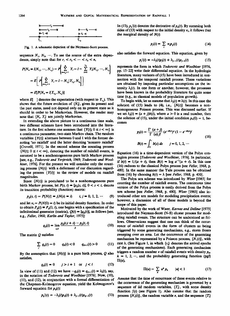
Fig. 1. A schematic depiction of the Neymann-Scott process.

In (13), p•(t) denotes the derivative ofp0(t ). By summing both sides of (13) with respect to the initial density •r,, it follows that the marginal density of N(t)

p;(t)-- • •ripi;(t) (14)

sequence N•, N,, -... To see the source of the extra dependence, simply note that for r• < r2 < -" < rk < n,

also satisfies the forward equation. This equation, given by

p/(t) -- --Xj(t)pj(t) + X;_l(t)p;_,(t) (15)

-- E[P(Nn -- l I Y•,•, N•)]

represents the form in which Todorovic and Woolhiser [1976, pp. 15-22] write their differential equation. In the hydrologic literature, many variants of (15) have been introduced in connection with the temporal rainfall process. These variations are obtained by imposing particular assumptions on the intensity X;(t). In one form or another, however, the processes have been known in the probability literature for quite some time (e.g., as classical models of population growth).

where E[ ] denotes the expectation (with respect to ¾rk). This To begin with, let us assume that 2¾( 0 -- 2•(t). In this case the shows that the future evolution of {N•}, given its present and solution of (15) leads to (4), i.e., {N(t)} becomes a non- the past states, need not depend only on its present state as it homogeneous Poisson process. This was discussed earlier. If should in order to be Markovian. However, the reader may we set X•(t) -- (a + j)b(t), where a > 0 is a real number, then note that {N•, Y•} are jointly Markovian. the solution of (15), under the initial condition po(0) -- 1, be-

In extending the above picture to a continuous time scale, comes two different schemes have been introduced into the litera-

ture. In the first scheme one assumes that {Y(t); 0 <_ t < oo} is a continuous parameter, two-state Markov chain. The random variables { Y(O} alternate between 0 and 1 with the former denoting 'no rainfall' and the latter denoting 'nonzero rainfall' [Crovelli, 1971]. In the second scheme the counting process {N(t); 0 <_ t < oo}, denoting the number of rainfall events, is assumed to be a nonhomogeneous pure birth Markov process [see, e.g., Todorovic and Yevjevich, 1969; Todorovic and Wool- hiser, 1976]. For the present we will consider only the counting process {N(t)} with a deferment of our discussion regarding the process {Y(t)} to the review of models on rainfall magnitudes.

Since {N(t)} is postulated to be a nonhomogeneous pure birth Markov process, let P(s, t) -- [p•s, t)], 0 < s < t, denote its transition probability (function) matrix:

p•(t) = r (a + j) (e_S(,)), (1 - r (a)fi

B(t) -- b(s) ds j-- O, 1, 2, ...

(16)

Equation (16) is a time-dependent version of the Polya con- tagion process [Todorovic and Woolhiser, 1976]. In particular, if b(t) -- 1/(a + O, then B(O -- log a-'(a + t). In this case (16) reduces to the classical Polya process [see Feller, 1968, p. 480]. In the same manner the Yule process can be obtained from (16) by choosing b(O -- X [see Feller, 1968, p. 450].

The Polya urn scheme was introduced by Wiser [1965] for counting the number of rainfall events. The continuous time version of the Polya process is easily derived from the Polya urn scheme [see Feller, 1968, p. 480]. Wiser [1965] also in-

po(s, t) = P(N(t) = jIN(s) = 0 i, j = 0, 1, 2, ... (9) troduced other urn models for modeling precipitation events; however, a discussion of all of these models is beyond the

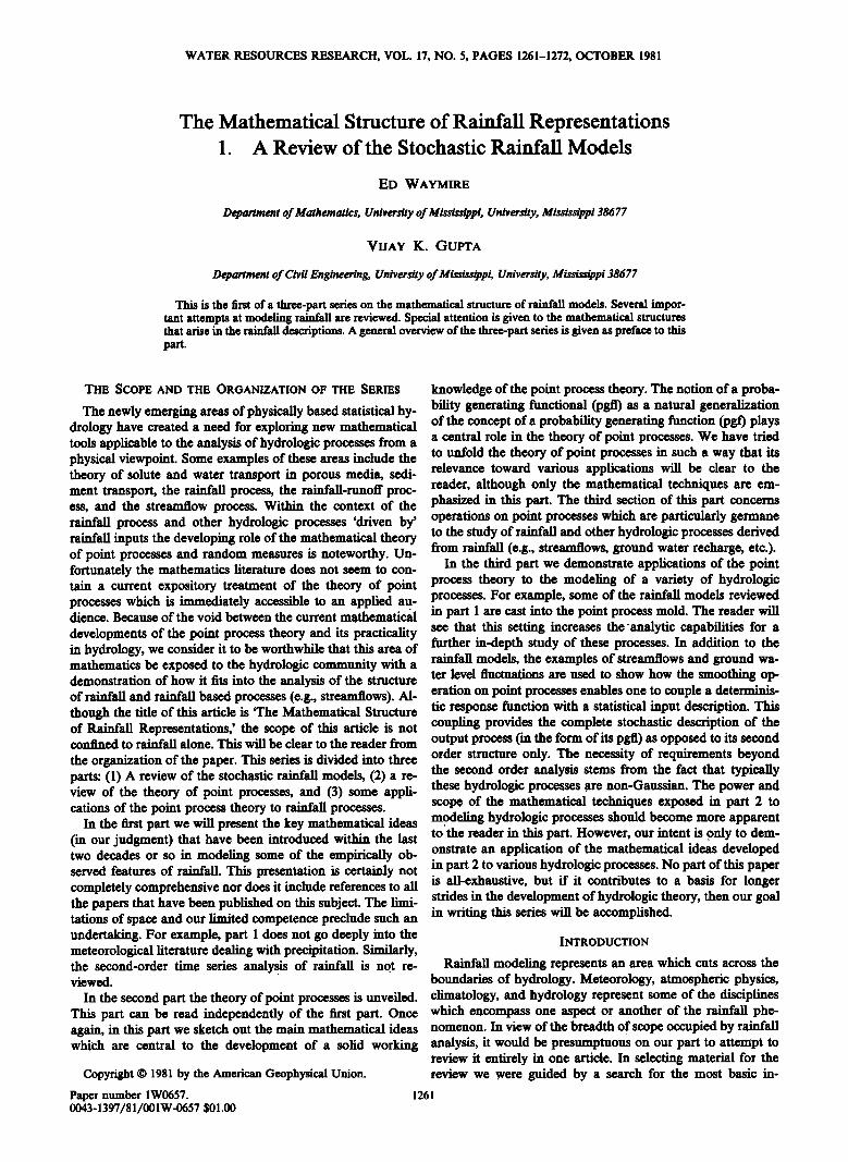
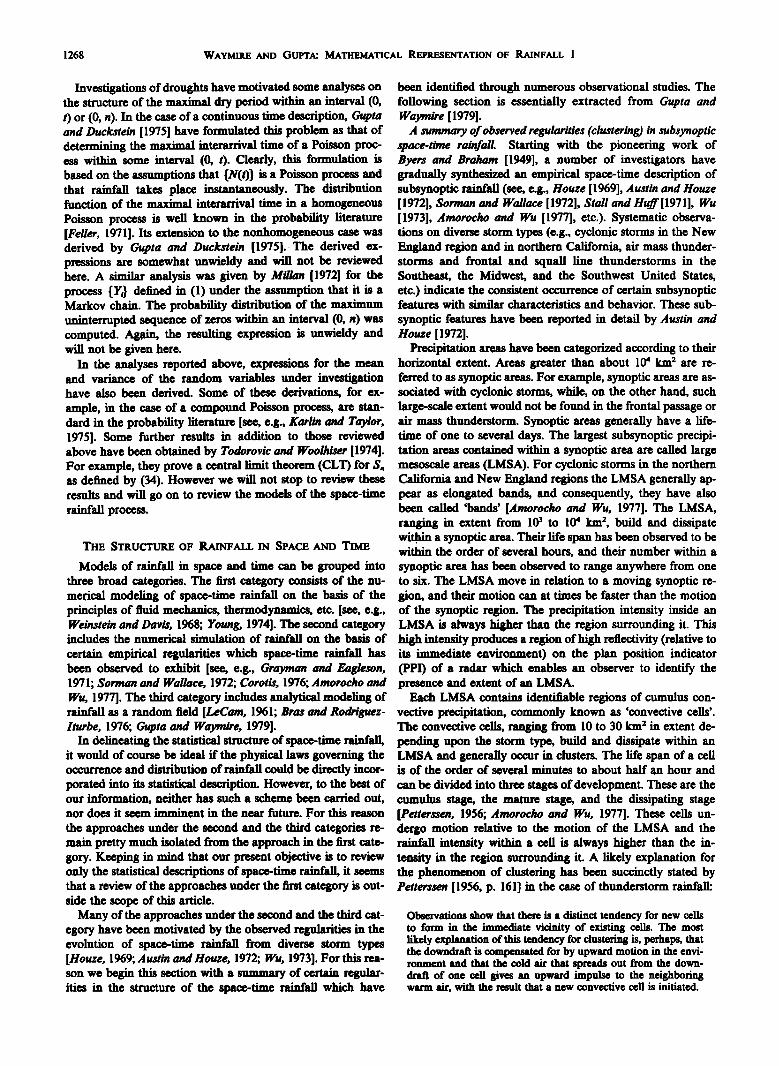
and let •r• = P(N(O) = 0 be its initial density function. In order scope of this paper. to obtain Po(t) • P•O, t), one begins with a specification of the Motivated by the work of Wiser, Kavvas and Delleur [1975] infinitesimal generator (matrix), Q(t) = [q•t)], as follows [see, introduced the Neyman-Scott (N-S) cluster process for mod- e.g., Feller, 1968; Karlin and Taylor, 1975]: cling rainfall events. The structure can be understood as fol-

lows. Observations suggest that one can think of the occur- qo(t)--lim p•t,t + s)-po(t, t) (10) rence of rainfall events in the form of clusters as being

s,o s triggered by some generating mechanisms, e.g., storm fronts The matrix Q satisfies sweeping over an area. Let the occurrence of the generating

mechanism be represented by a Poisson process, {NifO}, with

•. q•t) -- 0 qt,(t) < 0 qu+l(t) > 0 (11) rate 2•. (See Figure 1, in which {•-•} denotes the arrival epochs • of the generating mechanisms). Each generating mechanism

By the assumption that {N(t)} is a pure birth process, Q also triggers a random number v of rainfall events with density Pk, satisfies, k -- 1, 2, ..., and the probability generating function (pgf)

n(u), q•t)--O j>i+ 1 or j<i (12)

In view of (11) and (12) we have -qu(t) -- qu+•(t) -- X•(t), say, II(u) -- Y. lul < 1 (17) k

in the notation of Todorovic and Woolhiser [1976]. Now, (10), (11), and (12), in conjunction with a formal differentiation of Assume that the time of occurrence of these events relative to the Chapman-Kolmogorov equation, yield the Kolmogorov's the occurrence of the generating mechanism is governed by a forward equation for p•t): sequence of lid random variables, {T•}, with some density

function f(O. (see Figure 1). Also assume that the random pd(t) -- -X•(t)p•t) + X/_•(t)p•/_•(t) (13) process {NifO}, the random variable v, and the sequence {T•}

WAYMIRE AND GUFI'A: MATHEMATICAL REPRESENTATION OF RAINFALL I 1265

are independent. Let N(.O"- N(O, 0 denote the number of sequences • are usually within a continuous time frame rather rainfall events in (0, 0 and let •(u) denote the pgf of N(0. Then

q•t(u) m exp {-X f_'•(l-II[l-(1 .- u)•,(x)]) dx) /o" q,(x) - f (s - x)

(18)

h may be noted that q,,(x) represents the .probability that a rainfall event generated by a mechanism located at x occurs within the interval (0, t). Kavvas and Delleur [1975] also derived an expression for the joint pgf of N(t,) and N(t•), t, • t•, the number of rainfall events in (0, t•) and (0, t•), respectively. A comprehensive analysis of the rainfall process requires that the joint densities of N(t,) - N(t,_,), i • 1, 2, ..., n, t• • t• ... • t,, or their joint pgf be known [see, e.g., Kavvas and Delleur, 1975]. This is discussed systematically in part 2 of this. paper via more general transform techniques. An .application of the general transform for the N-S process derived 'm part 2 is given in part 3.

than in a discrete.time frame.

Grayman and Eagleson [1971] constructed sequences {T, (ø} and {Tb •ø} from rainfall records in the units of 10-minute in- cremems. A storm duration T, was defined as the duration of a sequence of rainfall bursts not separated .by more than two hours. The time between storms was defined as the sequence of zero rainfall intervals greater than two hours that separate two con•secutive rainfall bursts. They assumed that {T, <ø} are mutually independent and are independent of {Tbø)}. A Wei- bull 'density was fitted to {T, (0} and also .to {Tb<0}, the parameters.'of.the two .Weibull densities being different. More recently, Eagleson [1978] proposed the use of exponential densities with .'different parameters for the respective sequences of wet and dry.spells defined above. This postulate was supported by some rainfall data from Boston, Massach• setts.

The postulate s on {T, (')} and {Tb(0} made by Eagleson [1978] are a consequence of the Markovian assumption on the. continuous .t'tme analogue, {Y(t); 0 • t .< oo}, of the i&screte 'time: Markov cha'm { Y,; i--O}, Inthe continuous time version,

The above disc.USSion brings out the main ideaS that have. the g .eo-metric densities given by (20) and (21) become ex- been exploited 'm the hydrology literature for modeling the ponential, say With parameters X• and. X2, where I/X•_ is the counting processes assoc'mted with-the rainfall events.-Thus .mean •dry length and I/X• is the mean Wet length. The contin- far we have not considered other.important features of tern- uo .us-parameter Markov.c• { Y(t)} in the context of rainfall poral rainfall(e.g., the Structure ofr'alnfa!l .depthS, rainfall du- -has been explored by Crovelli [1971]. He gives.the expression ration, etc.)..These features will be considered now. for the transition density P(0 for. this Markov chain. Other .

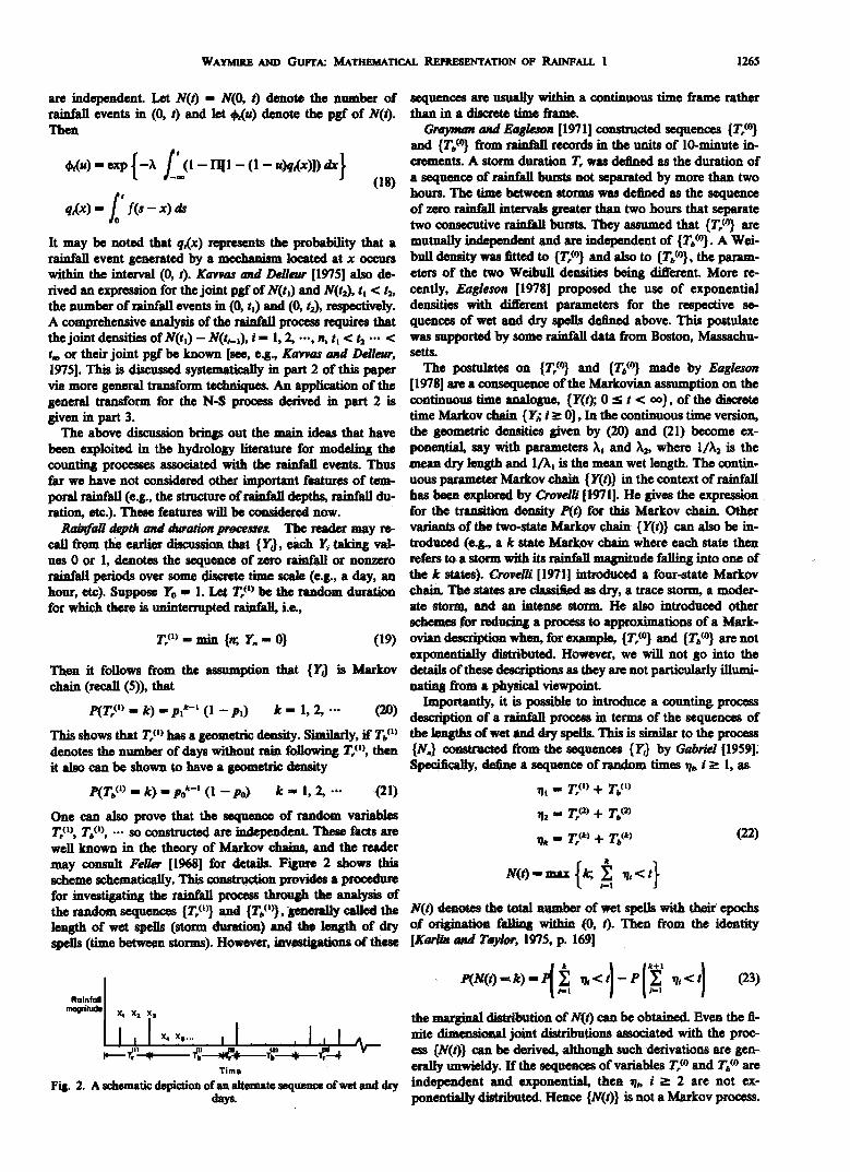
Rainfall depth and -duration processe..• The reader .may.re- variants 'ofthe't .wo-state Markov chain {Y(0} can alsO' .be in- call from .the earlier dtSCussion that' { Y,}, each •-tak' 'rag val' tr•oduCed (e,g., a k state Markov chain where each state ..then ues 0 or 1, denotes the sequence of zero ra'mfaH or nonzero refers. to a storm with.its ra'tnfaH magnitude-fa..11ing into one of r.ainfaH periods over some. :•ete .t:tme scale (e.g., a/daY, an' the. k states),•CroVelhi[ 197'1] introduced a four.state Markov ß hour,. e.•). SuP-pOse Yo" 1.. Let T,- be the random. dura•on chai n. 'The s•tes are class' ,trot as -.dry, a 'trace storm, a tooder- for which there is uninte•pted ra'mf•..i,e.,. ate storm, .and'an. intense storm. He al.so 'mtroduced. other

SChemes •forredu•g a. process -to approximations of a Mark- T?- .mitt {n; .Y, • 0} (19) ovian.description when, for example, {T? •} and (Tb (0} are.not

exponentially distributed. However, we will not go."mto the Then it follows from the assumption 'that (Y,} is Markov deta'ds of these descriptions as they are not particularly 'dlumi- chain (recall (5)), that hating .from a physical vie.wpoint.

Importantly, it-is possible to. introduce a count• process P(T? . k) ,= •'-' (1--p•) k = 1 2, .'- (20) description of a rainfall process in terms of the sequences of

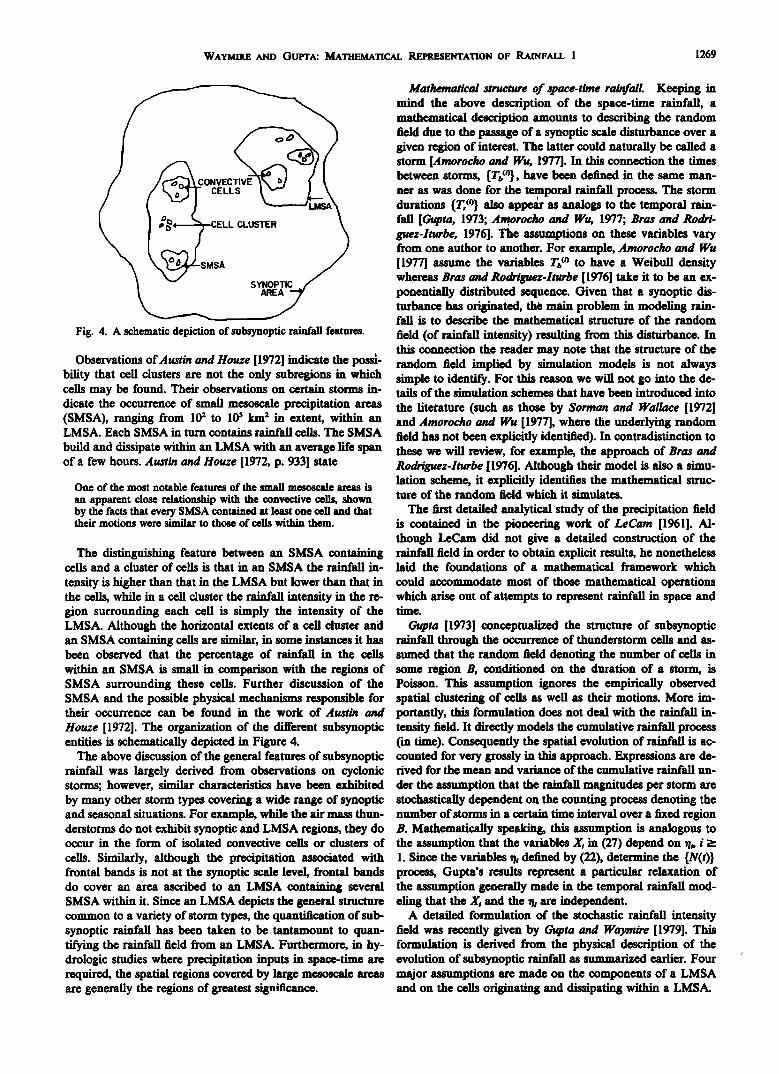
This shows that T? .has a geometric density. Similarly,/tf T•<O the lengths of wet .and dry spells. This is s'tmfiar to the process. denotes the n.um.•ber of days without ram follow'rag T?, then {N,} constructed. from the selquences {Y,} by .Gabriel [1959]. it also can be sho•wn to have a geometric density specifically, define a sequence of random times •,, i )_. 1, as

P(T•(O = k) m po •-• (I -Po) k =• 1, 2, .'- . '(21) • = T? + T• ø)

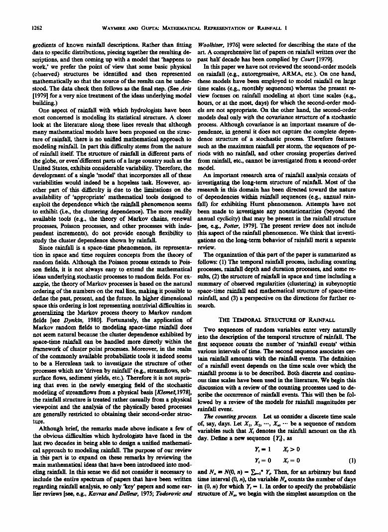
One can also prove .that the sequence of random variables T?, T• ø), .-. so constructed are. 'independent. These facts are well known in the theory of Markov cha'm s, and the reader may consult Feller [1968] for details, F'tgure 2' shows this SCheme schematically. T• construction provides a-p .rocedure for investigat'mg the rainfall process. thro-u• the analysis" of

',-, (l) the ran-do .m sequences t:/)- ] length of wet spells (storm duration) spells (time between sto/rms)..However, investigations of these

Rainfall/

Time

•2 = T.(•) + T? )

• = T?) + T•(,o (22)

N(t)•,max{k; • •,<t = ' ..N(0.•den'otes . -the total n/..••r of .wet s•Hs with theft .e•• of o .•mation f.'•g •bin (0, 0. Th• from •e -identity

P((0 '=k) = . . t.+. .

the. mar•aI •fibUfion of N(0 can • obtainS, Even the finite' .••iOn• jolt •distn•utions a• •at• with •e pr•- ess {N(t)) • be' derived, althou• such derivations •e gen- er•y •••Y, If the •ue•s of variables T• ø •d T• <ø are

.Fig. 2: A schematicdepi.CfionOfanalternatesequenceofwe t -and-dry rodepen.dent. land: exponential, then •,, i _) 2 are not ex- days. pon•nt:•y distributed. Hence {N(t)} 'LS not- a Markov process,

..

1266 WAYMIRE AND GUPTA: MATHEMATICAL REPRESENTATION OF RAINFALL I

,e._.Tl•) _(I) [,?.) {2) (.,.,T) -• T r = T,•---.>(-T•.-.-•.•Ti• ......

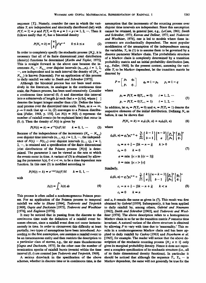
(different) exponential densities, Eagleson [1978] obtained an expression for the density of Xi in terms of the modified Bessel function of zero order. Interestingly enough, he showed that his data on rainfall magnitudes could be fitted well by this density as well as by a Gamma density, but not by an exponential density function. In contrast, the assumption of a common exponential density for the variables Xi has been exploited greatly by Todorovic and Yevjevich [1969] and Todo- rovic and Woolhiser [1976]. Before discussing their work we wish to remark that one obvious reason why an assumption

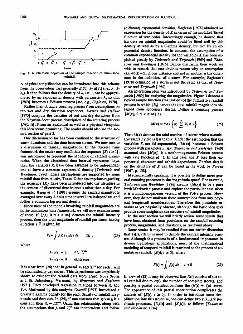
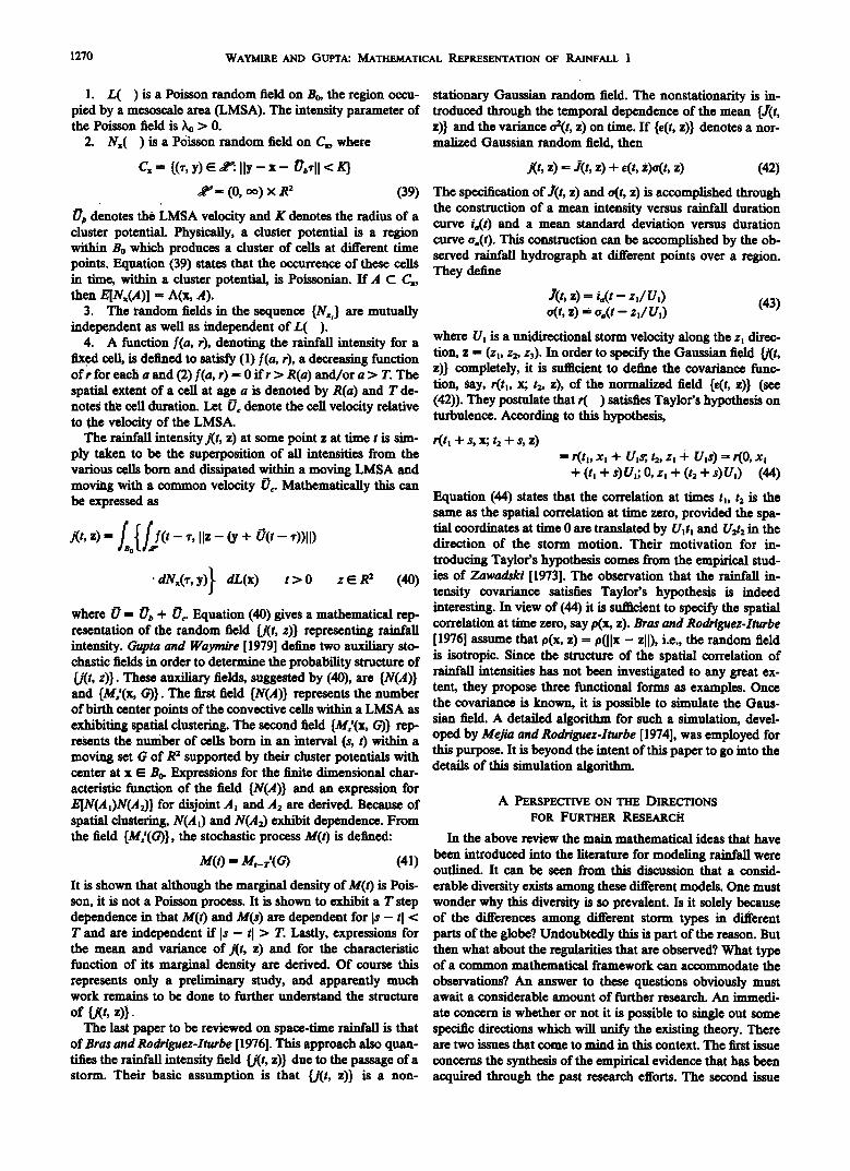
Fig. 3. A schematic depiction of the sample function of cumulative can work well in one instance and not in another is the differ-

rainfall. ence in the definitions of a storm. For example, Eagleson's A physical simplification can be introduced into this scheme [1978] definition of a storm is not the same as that of Todo-

rovic and Yevjevich [1969]. from the observation that generally E[Tb] >> E[T,] (i.e., 3• >> An interesting idea was introduced by Todorovic and Yev- 3•_). It then follows that the density of % i _> 1, can be approxi-

mated by an exponential density with parameters X•_ so that jevich [1969] for analyzing the magnitudes. Figure 3 denotes a {N(t)} becomes a Poisson process [see, e.g., Eagleson, 1978]. typical sample function (realization) of the cumulative rainfall

Rather than obtain a counting process from assumptions on the wet and dry duration sequences, Kavvas and Delleur [1975] compute the densities of wet and dry durations from the Neyman-Scott process description of the counting process {N(0, t)}. From an analytical as well as a physical viewpoint this idea seems promising. The reader should also see the sec-

process in which {Xi} denote the total rainfall magnitudes obtained from successive storms. Define a counting process {M(x), 0 _< x < oo} as

M(x) -- max {n; • X• < x} (2:5)

ond section of part 3. Then M(x) denotes the total number of storms whose cumula- Our discussion so far has been confined to the structure of tive rainfall yield is less than x. Under the assumption that the

storm durations and the time between storms. We now turn to variables X• are iid exponential, {M(x)} becomes a Poisson a discussion of rainfall magnitudes. In the discrete time framework the reader may recall that the sequence {X•; i _> 1}, was introduced to represent the sequence of rainfall magnitudes. When the discretized time interval represents days, then the variables Xt have been assumed to be independent and to have a common exponential density [Todorovic and Woolhiser, 1976]. These assumptions are supported by some rainfall data from Austin, Texas. Other assumptions regarding the sequence {XJ have been introduced into the literature in the context of discretized time intervals other than a day. For example, Wang et al. [1981] assume the rainfall magnitudes averaged over every 4-hour time interval are independent and follow a common log normal density.

Since most of the models involving rainfall magnitudes are in the continuous time framework, we will now examine some of these. If {j(s); 0 _< s < oo} denotes the rainfall intensity process, then the total magnitude of rainfall per storm having duration T, (ø is given by

Xi -- / j(s) Ir/o(s) ds i _> 1 (24) where

Ir?(s) -- 1 s • T• •ø

process with parameter/•, say. Todorovic and Yevjevich [1969] assumed that {M(x)} is a nonhomogeneous Poisson process with rate function/•( ). In this case, the X,. lose their exponential character and exhibit dependence. Further details on the structure of X• can be found in the work by Parzen [1967, p. 138].

Mathematically speaking, it is possible to define more general counting processes in the 'magnitude space'. For example, Todorovic and Woolhiser [1976] assume {M(x)} to be a pure birth Markovian process and explore the particular case when it is a nonhomogeneous version of the Polya process. How- ever, they do not motivate these assumptions from any physical (empirical) considerations. Therefore this postulate remains as yet physically obscure, although the basic idea may provide some insights on the structure of rainfall magnitudes.

In the next section we will briefly review some results that have been obtained from postulates on the rainfall counting process; magnitudes, and durations, as reviewed above.

Some results. It may be recalled from our earlier discussion that {j(s); s _> 0} is used to denote the rainfall intensity process. Although this process is of a fundamental importance in diverse hydrologic applications, most of the mathematical modeling of temporal rainfall is restricted to the process of cumulative rainfall, {X(0; t _> 0}, where

Ir/o(s) -- 0 otherwise

It is clear from (24) that in general X• and Tr (ø for each i will be stochastically dependent. This dependence was empirically shown to exist for the rainfall data from Truro, Nova Scotia and St. Johnsburg, Vermont, by Grayman and Eagleson [1971]. They developed regression relations between X, and Tr {ø. Motivated by this analysis, Crovelli [ 1971] introduced a bivariate gamma density for the joint density of rainfall mag-

t X(t) -- j(s) ds t _> 0 (26)

In view of (22) it may be observed that X(t) consists of the total rainfall due to N(t), the number of complete storms, and possibly a partial contribution from the (N(O + 1)st storm. The appearance of this partial contribution complicates the analysis of {X(t); t _> 0}. In order to introduce some sire-

nitude and duration. In (24), if one assumes that j(s) -- j• is a plification into this structure, one can define two auxiliary sto- constant, then X, --j,T• •ø. Using this relationship, along with chastic processes, {Xo(t)} and {X•(t)}, as follows [Todorovic the assumptions that j• and T• •ø are independent and follow and Woolhiser, 1976]:

WAYMIRE AND GUPTA.' MATHEMATICAL REPRESENTATION OF RAINFALL I 1267

Xo(t) -- • X, t _> 0 (27)

N•+I x,(o = x, t _> o (28)

It is clear from the above remarks that

Xo(0 -< X(t) _< X,(t) (29)

Now instead of investigating {X(0} directly, it becomes possible to investigate {Xo(0} as an approximation of {X(0 } . For the present we do not think it necessary to go into the details of this approximation. The interested reader may refer to Todorovic and Woolhiser [1976] as well as to some of Todo- rovic's earlier work referenced therein for further details. We will confine the ensuing discussion to considerations of {Xo(0}. The analysis of {X•(0} follows in a very similar man-

ner.

If Fo(x, 0 denotes the marginal distribution function of Xo(0, then in view of (27),

) Fo(x, 0 = = 0) + Y. X, < x, v(O = n (30) n--I i--I

Under the assumption that the variables X,. are iid and independent of {N(0}, and that {N(t)} is a Poisson process, (30) represents the distribution function of a compound Poisson process. This result has been rederived in the hydrologic literature at different times by different researchers [see, e.g., Le- Cam, 1961; Shane, 1964; Todorovic and Yevjevich, 1969; Duck- stein et al., 1972; and Eagleson, 1978]. In the case of a compound Poisson process, (30) reduces to

where

n Fo(x, t) -- e -^o) + •. F*n(x)e -A(') (31)

Under the assumptions that {M(x)} and {N(t)} are independent and that each is governed by a nonhomogeneous version of the Polya process, specific expressions for Fo(x, 0 have been obtained by Todorovic and Woolhiser [1976]. They also consider the discrete time version of cumulative rainfall process, Sn,

Sn= E X, + (34)

where the variables X, +, X: +, ... are lid with a common distribution given by the conditional distribution of X• given that {X, > 0}. It is important to note that in view of this assumption, the dependence in the sequence X,, X:, ... is only between the occurrence of wet and dry events and not between the rainfall magnitudes during wet periods. Todorovic and Woolhiser [1976] use (34) to derive an expression for the distribution of Sn, say F(x, n). The derivation also assumes that Nn is given by (6).

In the results quoted above attention is essentially focused on a derivation of the one dimensional (marginal) distribution of {Xo(0}. Since a stochastic process is determined by all its finite dimensional joint distribution functions, the above re- suits give only an incomplete description of the process {Xo(0}. An exception to this situation is represented by the compound Poisson process. Since the increments of this process are stochastically independent [Feller, 1968] its finite dimensional joint distributions can be written down immediately once its marginal distribution function Fo(x, t) is known. In addition to the cumulative rainfall process, two other processes derived from rainfall have been investigated. These we will now review.

Let Xo*(0 denote the maximal rainfall per rainfall storm in an interval (0, t). Then

Xo*(t)= max X, (35) I•/•r(t)

Under the assumption that the variables are lid and independent of {N(0 } , it follows that

and A(0 is as it was defined earlier in (4). Specific assumptions on the variables X, produce explicit and generally trac- table forms for Fo(X, t), the details of which need not detain us here.

From a physical viewpoint it can be seen that the above description of Xo(t) gives camouflage to some important features of rainfall (i.e., the storm duration and the 'distribution' of intensity over this duration). These features are not only essen- tial to a description of the rainfall intensity process, but also should play an important role in investigating the statistical behavior of, for example, the runoff process from a physical viewpoint. However, in some physical cases (e.g., in the case of summer thunderstorm rainfall in the Southwestern and the

Southeastern United States) it may be reasonable to assume that rainfall occurs instantaneously in clumps of size X•, i _> 1, as implied by the above description of Xo(0.

Some results beyond the compound Poisson description have .been derived from (30) by Todorovic and Woolhiser [1976]. In view of the counting process {M(x); x > 0} defined by (25), one can write (30) as

fo(X, 0 = eOv(o = o) + Y. Y. =j, v(O = n) n,=l jmn

(33)

P(Xo*(0 < x) = Fo*(X, 0 = • F•(x)P(N(t) = n) nmO

(36)

where F(x) denotes the common distribution function of X,, i -- 1, 2, -... This result was applied to thundersto• rainfall in the southwestern United States by Fogel and Duckstein [1969]. Its analogue for the case of a rainfall description over discretized time intervals (days) has been investigated by Todo- rovic and Woolhiser [1976]. In this case, if Xn •* denotes the maximal rainfall in n days, then

Zn *= max X, (37)

< x) = Y. F;(x)l0% =j) (38) j-o

Equation (38) is derived from the assumptions that the variables X, are iid and are independent of {Nn}. The two examples investigated by Todorovic and Woolhiser [1976] are for the two cases when Nn is given by (2) and (6). Once again the expressions given by (36) and (38) are only for the marginal distributions of the stochastic processes {Xo*(t); t > 0} and {Xn*; n _> 0}.

1268 WAYMIRE AND GUPTA: MATHEMATICAL REPRESENTATION OF RAINFALL I

Investigations of droughts have motivated some analyses on the structure of the maximal dry period within an interval (0, 0 or (0, n). In the case of a continuous time description, Gupta and Duckstein [1975] have formulated this problem as that of determining the maximal interarrival time of a Poisson process within some interval (0, 0. Clearly, this formulation is based on the assumptions that •N(0} is a Poisson process and that rainfall takes place instantaneously. The distribution function of the maximal interarrival time in a homogeneous Poisson process is well known in the probability literature [Feller, 1971]. Its extension to the nonhomogeneous case was derived by Gupta and Duckstein [1975]. The derived expressions are somewhat unwieldy and will not be reviewed here. A similar analysis was given by Millan [1972] for the process •Y,} defined in (1) under the assumption that it is a Markov chain. The probability distribution of the maximum uninterrupted sequence of zeros within an interval (0, n) was computed. Again, the resulting expression is unwieldy and will not be given here.

In the analyses reported above, expressions for the mean and variance of the random variables under investigation have also been derived. Some of these derivations, for ex-

ample, in the case of a compound Poisson process, are standard in the probability literature [see, e.g., Karlin and Taylor, 1975]. Some further results in addition to those reviewed above have been obtained by Todorovic and I•oolhiser [1974]. For example, they prove a central limit theorem (CLT) for $, as defined by (34). However we will not stop to review these results and will go on to review the models of the space-time rainfall process.

THE STRUCTURE OF RAINFALL IN SPACE AND TIME

Models of rainfall in space and time can be grouped into three broad categories. The first category consists of the numerical modeling of space-time rainfall on the basis of the principles of fluid mechanics, thermodynamics, etc. [see, e.g., Weinstein and Davis, 1968; Young, 1974]. The second category

been identified through numerous observational studies. The following section is essentially extracted from Gupta and Waymire [ 1979].

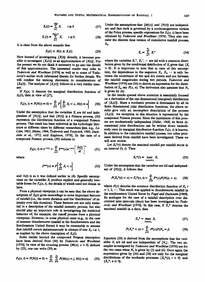
A •mmary of observed regularities (clustering) in •bsynoptic space-time rainfall. Starting with the pioneering work of Byers and Braham [1949], a number of investigators have gradually synthesized an empirical space-time description of subsynoptic rainfall (see, e.g., Houze [1969], Austin and Houze [1972], So.nan and Wallace [1972], Stall and Huff[1971], Wu [1973], Amorocho and Wu [1977], etc.). Systematic observations on diverse storm types (e.g., cyclonic storms in the New England region and in northern California, air mass thunderstorms and frontal and squall line thunderstorms in the Southeast, the Midwest, and the Southwest United States, etc.) indicate the consistent occurrence of certain subsynoptic features with similar characteristics and behavior. These sub-

synoptic features have been reported in detail by Austin and Houze [1972].

Precipitation areas have been categorized accor• to their horizontal extent. Areas greater than about 10 • km 2 are re- ferred to as synoptic areas. For example, synoptic areas are associated with cyclonic storms, while, on the other hand, such large-scale extent would not be found in the frontal passage or air mass thunderstorm. Synoptic areas generally have a life- time of one to several days. The largest subsynoptic precipitation areas contained within a synoptic area are called large mesoscale areas (LMSA). For cyclonic storms in the northern California and New England regions the LMSA generally appear as elongated bands, and consequently, they have also been called 'bands' [Amorocho and Wu, 1977]. The LMSA, ranging in extent from I(P to 10 • km 2, build and dissipate wit.hin a synoptic area. Their life span has been observed to be within the order of several hours, and their number within a synoptic area has been observed to range anywhere from one to six. The LMSA move in relation to a moving synoptic region, and their motion can at times be faster than the motion of the synoptic region. The precipitation intensity inside an LMSA is always higher than the region surrounding it. This

includes the numerical simulation of rainfall on the basis of high intensity produces a region of high reflectivity (relative to certain empirical regularities which space-time rainfall has its immediate environment) on the plan position indicator been observed to exhibit [see, e.g., Grayman and Eagleson, (PPI) of a radar which enables an observer to identify the 1971; So,nan and Wallace, 1972; Corotis, 1976; Amorocho and presence and extent of an LMSA. Wu, 1977]. The third category includes analytical modeling of Each LMSA contains identifiable regions of cumulus con- rainfall as a random field [LeCam, 1961; Bras and Rodriguez- vective precipitation, commonly known as 'convective cells'. Iturbe, 1976; Gupta and Waymire, 1979]. The convective cells, ranging from 10 to 30 km 2 in extent de-

In delineating the statistical structure of space-time rainfall, pending upon the storm type, build and dissipate within an it would of course be ideal if the physical laws governing the LMSA and generally occur in clusters. The life span of a cell occurrence and distribution of rainfall could be directly incor- is of the order of several minutes to about half an hour and porated into its statistical description. However, to the best of can be divided into three stages of development. These are the our information, neither has such a scheme been carried out, nor does it seem imminent in the near future. For this reason

the approaches under the second and the third categories remain pretty much isolated from the approach in the first category. Keeping in mind that our present objective is to review only the statistical descriptions of space-time rainfall, it seems

cumulus stage, the mature stage, and the dissipating stage [Petterssen, 1956; Amorocho and Wu, 1977]. These cells un- dergo motion relative to the motion of the LMSA and the rainfall intensity within a cell is always higher than the intensity in the region surrounding it. A likely explanation for the phenomenon of clustering has been succinctly stated by

that a review of the approaches under the first category is out- Petterssen [1956, p. 161] in the case of thunderstorm rainfall: side the scope of this article.

Many of the approaches under the second and the third category have been motivated by the observed regularities in the evolution of space-time rainfall from diverse storm types [Houze, 1969; •4ustin and Houze, 1972; I4Zu, 1973]. For this reason we begin this section with a su•mmary of certain regularities in the structure of the space-time rainfall which have

Observations show that there is a distinct tendency for new cells to form in the immediate vicinity of existing cells. The most likely explanation of this tendency for clustering is, perhaps, that the downdraft is compensated for by upward motion in the environment and that the cold air that spreads out from the downdraft of one cell sives an upward impulse to the neighborins warm air, with the result that a new convective cell is initiated.

WAYMIRE AND GUPTA: MATHEMATICAL REPRESENTATION OF RAINFALL I 1269

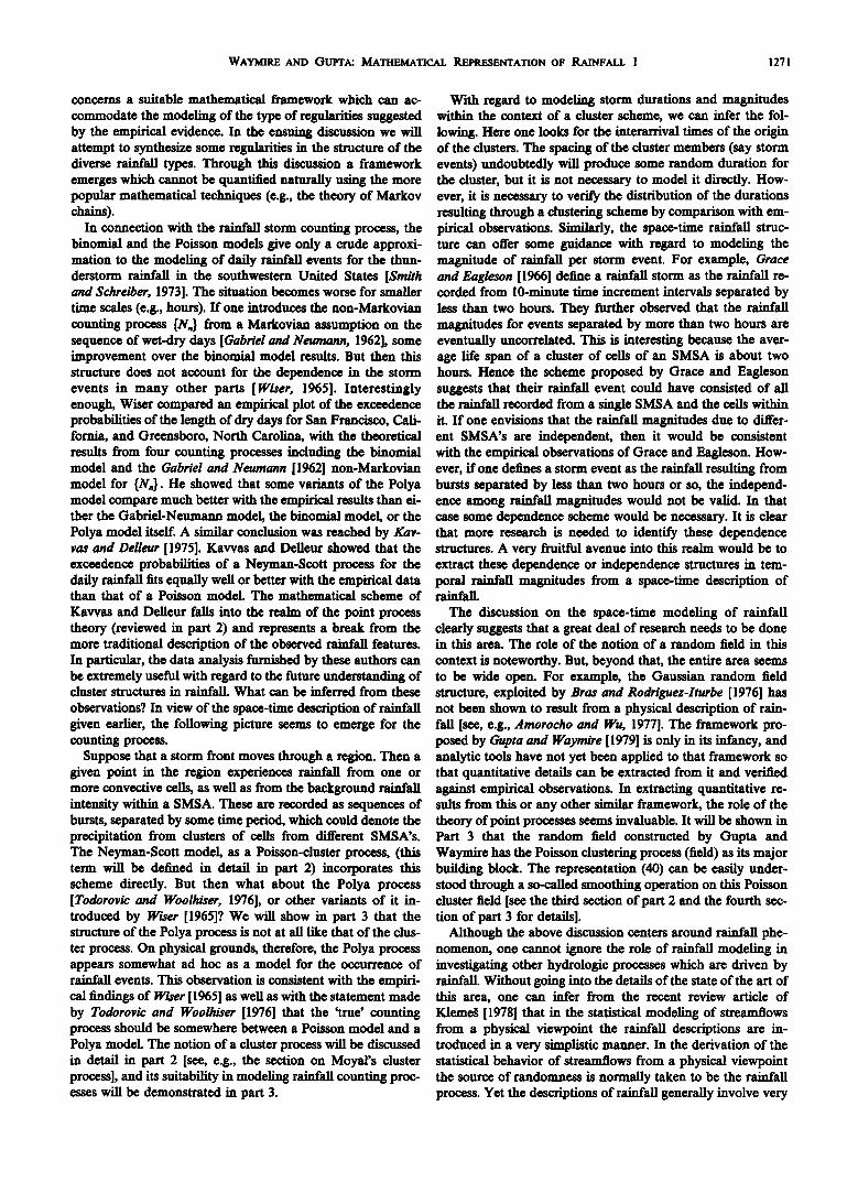
Fig. 4. A schematic depiction of subsynoptic rainfall features.

Observations of Austin and Houze [1972] indicate the possi- bility that cell clusters are not the only subregions in which cells may be found. Their observations on certain storms in- dieate the occurrence of small mesoscale precipitation areas (SMSA), ranging from 10 • to 103 km 2 in extent, within an LMSA. Each SMSA in turn contains rainfall cells. The SMSA

build and dissipate within an LMSA with an average life span of a few hours. Austin and Houze [1972, p. 933] state

One of the most notable features of the small mesoscale areas is

an apparent close relationship with the convective cells, shown by the facts that every SMSA contained at least one cell and that their motions were similar to those of cells within them.

The distinguishing feature between an SMSA containing cells and a cluster of cells is that in an SMSA the rainfall in-

tensity is higher than that in the LMSA but lower than that in the cells, while in a cell cluster the rainfall intensity in the region surrounding each cell is simply the intensity of the LMSA. Although the horizontal extents of a cell cluster and

Mathematical structure of space-time rainfall. Keeping in mind the above description of the space-time rainfall, a mathematical description amounts to describing the random field due to the passage of a synoptic scale disturbance over a given region of interest. The latter could naturally be called a storm [Amorocho and lgu, 1977]. In this connection the times between storms, {T b(ø}, have been defined in the same manner as was done for the temporal rainfall process. The storm durations {T• (ø} also appear as analogs to the temporal rainfall [Gupta, 1973; Amorocho and lgu, 1977; Bras and Rodri- guez-Iturbe, 1976]. The assumptions on these variables vary from one author to another. For example, Amorocho and [1977] assume the variables Tb (ø to have a Weibull density whereas Bras and Rodriguez-Iturbe [ 1976] take it to be an exponentially distributed sequence. Given that a synoptic disturbance has originated, the main problem in modeling rainfall is to describe the mathematical structure of the random

field (of rainfall intensity) resulting from this disturbance. In this connection the reader may note that the structure of the random field implied by simulation models is not always simple to identify. For this reason we will not go into the details of the simulation schemes that have been introduced into

the literature (such as those by Sorman and Wallace [1972] and Amorocho and W'u [1977], where the underlying random field has not been explicitly identified). In contradistinction to these we will review, for example, the approach of Bras and Rodriguez-Iturbe [1976]. Although their model is also a simulation scheme, it explicitly identifies the mathematical structure of the random field which it simulates.

The first detailed analytical study of the precipitation field is contained in the pioneering work of LeCam [1961]. Al- though LeCam did not give a detailed construction of the rainfall field in order to obtain explicit results, he nonetheless laid the foundations of a mathematical framework which

could accommodate most of those mathematical operations which arise out of attempts to represent rainfall in space and time.

Gupta [1973] conceptualized the structure of subsynoptic an SMSA containing cells are similar, in some instances it has rainfall through the occurrence of thunderstorm cells and as- been observed that the percentage of rainfall in the cells sumed that the random field denoting the number of cells in within an SMSA is small in comparison with the regions of some region B, conditioned on the duration of a storm, is SMSA surrounding these cells. Further discussion of the Poisson. This assumption ignores the empirically observed SMSA and the possible physical mechanisms responsible for spatial clustering of cells as well as their motions. More ira- their occurrence can be found in the work of Austin and portantly, this formulation does not deal with the rainfall in- Houze [1972]. The organization of the different subsynoptic tensity field. It directly models the cumulative rainfall process entities is schematically depicted in Figure 4. (in time). Consequently the spatial evolution of rainfall is ac-

The above discussion of the general features of subsynoptic counted for very grossly in this approach. Expressions are de- rainfall was largely derived from observations on cyclonic rived for the mean and variance of the cumulative rainfall un- storms; however, similar characteristics have been exhibited der the assumption that the rainfall magnitudes per storm are by many other storm types covering a wide range of synoptic stochastically dependent on the counting process denoting the and seasonal situations. For example, while the air mass thun- number of storms in a certain time interval over a fixed region derstorms do not exhibit synoptic and LMSA regions, they do B. Mathematically speaking, this assumption is analogous to occur in the form of isolated convective cells or clusters of the assumption that the variables X, in (27) depend on % i _• cells. Similarly, although the precipitation associated with 1. Since the variables •/, defined by (22), determine the {N(t)} frontal bands is not at the synoptic scale level, frontal bands process, Gupta's results represent a particular relaxation of do cover an area ascribed to an LMSA containing several the assumption generally made in the temporal rainfall mod- SMSA within it. Since an LMSA depicts the general structure cling that the X, and the •/, are independent. common to a variety of storm types, the quantification of sub- A detailed formulation of the stochastic rainfall intensity synoptic rainfall has been taken to be tantamount to quan- field was recently given by Gupta and Waymire [1979]. This tifying the rainfall field from an LMSA. Furthermore, in hy- formulation is derived from the physical description of the drologic studies where precipitation inputs in space-time are evolution of subsynoptic rainfall as s_u_mmarized earlier. Four required, the spatial regions covered by large mesoscale areas major assumptions are made on the components of a LMSA are •enerallv the regions of greatest si•,nificance_ nnrl on th,. cells o•ginating and '•' o•..o+- _ . _ _ __.. ............ XSo,t,,,•tng within a LMSA.

1270 WAYMIRE AND GUPTA.' MATHEMATICAL REPRESENTATION OF RAINFALL I

1. L( ) is a Poisson random field on Bo, the region occu- stationary Gaussian random fieldß The nonstationarity is in- pied by a mesoscale area (LMSA). The intensity parameter of troduced through the temporal dependence of the mean {J(t, the Poisson field is Xo > 0. z)} and the variance o2(t, z) on time. If {e(t, z)} denotes a nor-

2. Nx( ) is a Poisson random field on Cx, where malized Gaussian random field, then

C,, -- {0', Y) E • I ly - x - Oowll </q j(t, z) = J(t, z) + z)o(t, z) (42)

•'-- (0, oo) x R 2 (39)

/•b denotes the LMSA velocity and K denotes the radius of a cluster potential. Physically, a cluster potential is a region within Bo which produces a cluster of ce'ils at different time points. Equation (39) states that the occurrence of these cells in time, within a cluster potential, is Poissonian. If ,4 C C•, then E[Nx(A)] = A(x, A).

3. The random fields in the sequence {N•,,} are mutually independent as well as independent of L( ).

4. A function f(a, r), denoting the rainfall intensity for a fixed cell, is defined to satisfy (I) f(a, r), a decreasing function of r for each a and (2) f(a, r) = 0 if r > R(a) and/or a > T. The spatial extent of a cell at age a is denoted by R(a) and T denotes th• cell duration. Let •½ denote the cell velocity relative to the velocity of the LMSA.

The rainfall intensity j(t, z) at some point z at time t is simply taken to be the superpositi0n of all intensities from the various cells born and dissipated within a moving LMSA and moving with a common velocity U½. Mathematically this can be expressed as

j(t, z)-- f• {f•f(t-•', ][z- (y + O(t- ,))]1) o

ß dN,,O', y)} dL(x) t > 0 z tE R'- (40) where • = 0b + •½. Equation (40) gives a mathematical representation of the random field {j(t, z)} representing rainfall intensity. Gupta and Waymire [1979] define two auxiliary stochastic fields in order to determine the probability structure of

The specification of J(t, z) and o(t, z) is accomplished through the construction of a mean intensity versus rainfall duration curve ia(0 and a mean standard deviation versus duration curve oa(t). This construction can be accomplished by the observed rainfall hydrograph at different points over a region. They define

J(t, z) --- i.(t - z,/ UO (43) o(t, z) --- o•(t - z,/ U,)

where Ul is a unidirectional storm velocity along the zl direction, z -- (zl, z,, z3). In order to specify the Gaussian field {j(t, z)} completely, it is sufficient to define the covariance function, say, r(tl, x; t2, z), ½f the normalized field {e(t, z)} (see (42)). They postulate that r( ) satisfies Taylor's hypothesis on turbulence. According to this hypothesis,

r(t, + s, x; t,_ + s, z) -- r(t,, X 1 + Ul$; t2, Z 1 + Ui$ ) ----- r(0, X 1

+ (tl + s)U,; O, Zl + (t: + $)Ui) (44)

Equation (44) states that the correlation at times tl, t,_ is the same as the spatial correlation at time zero, provided the spatial coordinates at time 0 are translated by Ult, and U,_t,_ in the direction of the storm motion. Their motivation for in-

troducing Taylor's hypothesis comes from the empirical studies of Zawadski [1973]. The observation that the rainfall intensity covariance satisfies Taylor's hypothesis is indeed interesting. In view of (44) it is sufficient to specify the spatial correlation at time zero, say p(x, z). Bras and Rodriguez-Iturbe [1976] assume that p(x, z) -- (llx - zll), i.e., the random field is isotropic. Since the structure of the spatial correlation of

{j(t, z)}. These auxiliary fields, suggested by (40), are {N(A)} rainfall intensities has not been investigated to any great ex- and {Md(x, G)}. The first field {N(A)} represents the number tent, they propose three functional forms as examples. Once

the covariance is known, it is possible to simulate the Gaus- of birth center points of the convective cells within a LMSA as sian field. A detailed algorithm for such a simulation, devel- exhibiting spatial clustering. The second field {Md(x, G)} rep-

resents the number of cells born in an interval (s, 0 within a oped by Mefia and Rodriguez-Iturbe [1974], was employed for this purpose. It is beyond the intent of this paper to go into the moving set G of ll• 2 supported by their cluster potentials with

center at x E Bo. Expressions for the finite dimensional characteristic function of the field {N(A)} and an expression for E[N(Ai)N(A,)] for disjoint ,4, and A2 are derived. Because of spatial clustering, N(,41) and N(A,) exhibit dependence. From the field {Ms'(G)}, the stochastic process M(0 is defined:

M(0 --- M,_r'(G) (41)

It is shown that although the marginal density of M(0 is Pois- son, it is not a Poisson process. It is shown to exhibit a T step dependence in that M(0 and M(s) are dependent for I s - t I <

details of this simulation algorithm.

A PERSPECTIVE ON THE DIRECTIONS

FOR FURTHER RESEARCH

In the above review the main mathematical ideas that have

been introduced into the literature for modeling rainfall were outlined. It can be seen from this discussion that a consid-

erable diversity exists among these different models. One must wonder why this diversity is so prevalent. Is it solely because of the differences among different storm types in different

T and are independent if [s - tl > T. Lastly, expressions for parts of the globe? Undoubtedly this is part of the reason. But the mean and variance of j(t, z) and for the characteristic function of its marginal density are derived. Of course this represents only a preliminary study, and apparemly much work remains to be done to further understand the structure

of {j(t, z)}. The last paper to be reviewed on space-time rainfall is that

of Bras and Rodriguez-Iturbe [1976]. This approach also quan-

then what about the regularities that are observed? What type of a common mathematical framework can accommodate the

observations? An answer to these questions obviously must await a considerable amount of further research. An immedi-

ate concern is whether or not it is possible to single out some specific directions which will unify the existing theory. There are two issues that come to mind in this context. The first issue

titles the rainfall intensity field {.j(t, z)} due to the passage of a concerns the synthesis of the empirical evidence that has been storm. Their basic assumption is that {j(t, z)} is a non- acquired through the past research efforts. The second issue

WAYMIRE AND GUPTA: MATHEMATICAL REPRESENTATION OF RAINFALL 1 1271

concerns a suitable mathematical framework which can ac-

commodate the modeling of the type of regularities suggested by the empirical evidence. In the ensuing discussion we will attempt to synthesize some regularities in the structure of the diverse rainfall types. Through this discussion a framework emerges which cannot be quantified naturally using the more popular mathematical techniques (e.g., the theory of Markov chains).

In connection with the rainfall storm counting process, the binomial and the Poisson models give only a crude approximation to the modeling of daily rainfall events for the thunderstorm rainfall in the southwestern United States [Smith and Schreiber, 1973]. The situation becomes worse for smaller time scales (e.g., hours). If one introduces the non-Markovian counting process {Nn} from a Markovian assumption on the sequence of wet-dry days [Gabriel and Neumann, 1962], some improvement over the binomial model results. But then this structure does not account for the dependence in the storm events in many other parts [Wiser, 1965]. Interestingly enough, Wiser compared an empirical plot of the exceedence probabilities of the length of dry days for San Francisco, Cali-

With regard to modeling storm durations and magnitudes within the context of a cluster scheme, we can infer the following. Here one looks for the interarrival times of the origin of the clusters. The spacing of the cluster members (say storm events) undoubtedly will produce some random duration for the cluster, but it is not necessary to model it directly. How- ever, it is necessary to verify the distribution of the durations resulting through a clustering scheme by comparison with empirical observations. Similarly, the space-time rainfall structure can offer some guidance with regard to modeling the magnitude of rainfall per storm event. For example, Grace and œagleson [1966] define a rainfall storm as the rainfall recorded from 10-minute time increment intervals separated by less than two hours. They further observed that the rainfall magnitudes for events separated by more than two hours are eventually uncorrelated. This is interesting because the average life span of a cluster of cells of an SMSA is about two hours. Hence the scheme proposed by Grace and Eagleson suggests that their rainfall event could have consisted of all the rainfall recorded from a single SMSA and the cells within it. If one envisions that the rainfall magnitudes due to differ-

fornia, and Greensboro, North Carolina, with the theoretical ent SMSA's are independent, then it would be consistent results from four counting processes including the binomial with the empirical observations of Grace and Eagleson. How- model and the Gabriel and Neumann [1962] non-Markovian ever, if one defines a storm event as the rainfall resulting from model for {Nn}. He showed that some variants of the Polya bursts separated by less than two hours or so, the independ- model compare much better with the empirical results than ei- ther the Gabriel-Neumann model, the binomial model, or the Polya model itseft. A similar conclusion was reached by Kav- vas and Delleur [1975]. Kavvas and Delleur showed that the exceedence probabilities of a Neyman-Scott process for the daily rainfall fits equally well or better with the empirical data

ence among rainfall magnitudes would not be vahd. In that case some dependence scheme would be necessary. It is clear that more research is needed to identify these dependence structures. A very fruitful avenue into this realm would be to extract these dependence or independence structures in temporal rainfall magnitudes from a space-time description of

than that of a Poisson model. The mathematical scheme of rainfall.

Kavvas and Delleur falls into the realm of the point process The discussion on the space-time modeling of rainfall theory (reviewed in part 2) and represents a break from the clearly suggests that a great deal of research needs to be done more traditional description of the observed rainfall features. in this area. The role of the notion of a random field in this In particular, the data analysis furnished by these authors can context is noteworthy. But, beyond that, the entire area seems be extremely useful with regard to the future understanding of to be wide open. For example, the Gaussian random field cluster structures in rainfall. What can be inferred from these structure, exploited by Bras and l•odriguez-Iturbe [1976] has observations? In view of the space-time description of rainfall not been shown to result from a physical description of rain- given earlier, the following picture seems to emerge for the fall [see, e.g., Amorocho and Wu, 1977]. The framework pro- counting process. posed by Gupta and Waymire [1979] is only in its infancy, and

Suppose that a storm front moves through a region. Then a analytic tools have not yet been applied to that framework so given point in the region experiences rainfall from one or that quantitative details can be extracted from it and verified more convective cells, as well as from the background rainfall against empirical observations. In extracting quantitative re- intensity within a SMSA. These are recorded as sequences of suits from this or any other similar framework, the role of the bursts, separated by some time period, which could denote the precipitation from clusters of cells from different SMSA's. The Neyman-Scott model, as a Poisson-cluster process, (this term will be defined in detail in part 2) incorporates this scheme directly. But then what about the Polya process [Todorovic and Woolhiser, 1976], or other variants of it introduced by Wiser [1965]? We will show in part 3 that the structure of the Polya process is not at all like that of the cluster process. On physical grounds, therefore, the Polya process appears somewhat ad hoc as a model for the occurrence of rainfall events. This observation is consistent with the empirical findings of Wiser [1965] as well as with the statement made by Todorovic and Woolhiser [1976] that the 'true' counting process should be somewhere between a Poisson model and a Polya model. The notion of a cluster process will be discussed in detail in part 2 [see, e.g., the section on Moyal's cluster process], and its suitability in modeling rainfall counting processes will be demonstrated in part 3.

theory of point processes seems invaluable. It will be shown in Part 3 that the random field constructed by Gupta and Waymire has the Poisson clustering process (field) as its major building block. The representation (40) can be easily understood through a so-called smoothing operation on this Poisson cluster field [see the third section of part 2 and the fourth section of part 3 for details].

Although the above discussion centers around rainfall phenomenon, one cannot ignore the role of rainfall modeling in investigating other hydrologic processes which are driven by rainfall. Without going into the details of the state of the art of this area, one can infer from the recent review article of Kleme• [1978] that in the statistical modeling of streamflows from a physical viewpoint the rainfall descriptions are introduced in a very simplistic manner. In the derivation of the statistical behavior of streamflows from a physical viewpoint the source of randomness is normally taken to be the rainfall process. Yet the descriptions of rainfall generally involve very

1272 WAYMIRE AND. GUPTA: •dATHEMATICAL REP•SE'•A•ON OF RAINFALL 1

strong assumptions (e.g., that the sequence of r•faH-'.ma -•i- Gu•,- V. K., and E. C. Waymire, A stochastic. kinematic study of tUd es is lid). These assumptions 'are di.ctated more by the . subsynoptic.space.timerainfaH,'WaterResour. ReS•,15(3), 637•, ChOice of mathe-marital tools (e.g., an' autoregressive, a moving average, or an ARMA model) than by the .Physical de, scription of rainfall. It will be shown in part 3 that a 'coupling' of a realistic stochastic description of rainfall with that of a r'ainfaH-runoff transformation leads to the point process. framework. This, by the way, was first re'-.alized by LeCam [1961].

Acknowledgment. This research was supponed• by the National Science.Foundation Grant CME-7907793.

REFERENCES

Amorocho, J., and B. 'Wu, Mathematical models for the simulation of cyclonic storm sequences and precipitation fields, Y. HYdrol., 32, 329-345, 1977.

ß Aris, R., Mathematical Modelling Technfitues, Res. Notes in Math., vol. 24, Pitman, San Francisco, 1979:.

Austin, P.M., and R. A. Houze, Jr., Analysis .of the structure of pre, cipitation patterns in New England, J. Appl. Meterol., 11' 926--934, 1972.

Bras, R., and I. Rodriguez-Iturbe, Rainfall generation: A. non- stationary .'tune v .arying multidimensional model, Water Resour.

1979,

Houze, R. A., Jr., •racteristiCs of mesoscale precipitation areas, M. S. Thesis,• Dep. of Meteorel., Mass. Inst. of Technol., Cambridge, Mass., 1969.

Karlin, S., and H. M. Taylor, A First Course in Stochastic Processes, Academic, New York, 1975.

Kavvas, L., and J. W. Dellcur, The stochastic and chronological structure of rainfall sequences: Application to Indiana, Water Resour. Res. Center Rep. 57' 'PurdUe Univ., West Lafayette, Ind., 1975.

Kleme•, V., Physically based stoc •hastic hydrologic analysis, Adv. Hy- drosci., 11, 285-352, New York, 1978.

LeCam, L., A stochastic description of precipitation, paper presented at 'the Fourth Berkeley Symposium on Mathematics, Statistics, and Probability, Univ. of Calif., Berkeley, Calif., 1961.

Mejia, J. M., and I. RodrigueZ-Iturbe, On the synthesis of random field sampling from the spectrum: An application to the generation of hydro10gic spatial processes, Water Resour. Res., 10(4), 705-711, 1974.

Millan, J., Drought impact on regional economy, Hydrol. Pap• 55, COlo. State Univ., Fort Collins, 1972.

Parzen, E,, Stochastic Processes, Holden-Day, San Francisco, 1967. Petterssen, S., Weather Anal)sis and Forecasting, vol. 2, McGraw-Hill,

New York, 1.956. Potter, K. W., Annual precipitation 'm the Northeast United States:

Long memory, short'memory, or no-memory?, Water Resour. Res., 15(2), "3,d)-346, 1979.

Res., •2(3), 450-456, 1976. _ ... Shane, R. M,, The application of the compound Poisson .distribution Byers, H. R., and R. R. Braham, The thunderstorm, in ' ß ' to 'the analysis of the rainfall ecor•ds, M.S. thesis, Cornell Univ., Report oJ- ttte . r

Thunderstorm Project,. U,S, Weather Bureau, Washington" D, C., 'Ithaca, New York, 1964. :' 1949. Smith, R. E., and H. A, Schreiber, . Point pr :ocess of seasonal thunder- .Caskey, I.E., Jr., A Markov Chain model for the probability..•r- storm r 'am/all, 1, D•bution of-. events, Water Resour. Res.,

rence in interval of Various length, Month. Weather Rev.,. 91, 289- 9(4), 871-884, 1973. 301, 1963. So.rman, U. A., and J. R. Wallace,. Digital s'maulation of thunderstorm

Corotis, R. B., Stochastic considerations in thunderstorm modeling, J. .rainfall, Partial Completion Rep. 0 WRR-A-O36-GA, Environ• Re- Ilydraul. Div. Am. Soc. CiV. Eng., 102(HY7), 865-878, 1976i' sour. Center, Georgia Inst. Technol., Atlanta, 1972.

'Court, A., Precipitation research, 19.75-1978, Rev. Geophys, Space Stall, i. B., and F. A. Huff, The structure of thunderstorm r 'arefall, pa- Phys., 17(6), 1165-1175, 1979. .per presented at the National Water Resources Engineering Meet•

Crovelli, R. A., Stochastic models for precipitation, Ph.D. diS, '.tug, Am. Soc, Civ. Eng., PbGC'nix, "'Ariz., 1971. sertation, Dep. of StatistiC, Colo. State Univ., Fort Collins, 1'97 I. Todorovic, P., and D. A. Woolhi.set,-Stochastic model of d•ly rain-

Duckstein, L., M.' M.'Fogel, 'and C. C. Kisiel, A stochastic'model :of fall, USDA Misc. Publ. U.S. Dep..Agric., 1275, 232-246, 1974. runoff-producing r-'•n.fall for summer tYPe storms,. Water Resour' Todorovic, P., and D. A. Woo-•er, Stochastic structure of the local Res, 8(2), 410-421, 1972. Dynkin= E. B., Markov processes and Random fields, Bull. Ant Math, • :.pattern of precipitation, in Stochastic Approaches to Water Re- sources, vol 2, edited by H.W..Shen, Colorado State University, $oc., 3(3), 975-999, 1980. FOrt Collins, Colo., 1976.

Eagleson, P., Climate, soil, and vegetation, 2, The distribution of an- Todorovic, P., and V. Yevjevich, Stochastic process of precipitation,, nual precipitation derived from observed storm sequences, Water .- . Hydrol. Pap. 35, Colo. State UniV., Fort Collins, 1969. Resour. Res., 14(5), 713-721, 1.978. Wang, C. T., V. K. Gupta, and E• :-Waymire, A geomorphologic syn-

Feller, W., An Introduction to Probability Theory and its Applicat'ions,: . '.thesis of nonlinearity in surfa ce runoff, Water Resour. Res., 17(3), vol. 1, John Wiley, New York, 1968. -- 545-554, 1981.

Feller, W., An Introduction to Probability Theory and its Applications, Waymire, E., and V. K. Gupta, The mathematical structure of rainfall vol. 2, John Wiley, New York, 1971. representations, 2, A review of the theory of point processes, Water

Feyerherm, A.M., L. D. Bark, and W. C. Burrows, Probabilities of se- Resour. Res., this issue. quences of wet and dry days in Indiana, Teck Bull. 13õf, Agdc, Waymire, E., and V. K. Gupta, The mathematical structure of r 'arefall Exp. Stn., Kansas State. Univ., Manhattan, Kansas, 1965. representations, 3, Some applications of the point process theory to

Fogel, M. M., and L. Duckstein, Point rainfall frequency in con- rainfall processes, Water Resour• Re•, this issue. vective storms, Water Resour. Res., 5(6), 1229-1237, 1969. Weinstein, A. I., and L. G. Davis, A parameterized numerical model

Gabriel, K. R., The distribution of the number of successes in'a se- of cumulus convection, Report 2 to the National Science Founda- quence of dependent trialS, Biometrika, 96, 454-460, 1959. tion, Penn. State Univ., University Park, 1968.

Gabriel, K. R., and J.. Neumann, A Markov Chain model for daily Wiser, E. H., Modified Markov..probability models of sequences of rainfall occurrences at Tel-Aviv, Q. J. R. Meteorel. Sac., 88, .90-85, precipitation events, Men. Weather Rev.,-93, 511-516, 1965. 1962.

Grace, R. A., and P.S. Eagleson, The synthesis of short-time increment rainfall sequences, Hydrodyn. Lab. Rep. 91, Mass. Inst. of Technol., Cambridge, Mass., 1966.

Grayman, W. M., and P.S. Eagleson, Evaluation of radar and rain. gage systems for flood forecasting, R-M.P. Lab. Rep. 138, Mass.. Inst. of Technol., Cambridge, Mass., 1971.

Gupta, V. K., A stochastic approach to space-time modeling of rainfall, Tech. Rep. Nat. Resour. Syst. 18, Dep. of Hydrol. and Water Resour., Univ. of Ariz., Tucson, 1973.

Gupta, V. K., and L. Duckstein, A stochastic a_nalysis of extreme droughts, Water Resour. Res.,' 11(2), 221-228, 1975.

Wu, B., Mathematical models for the simulation of cyclonic storm sequences and precipitation fields, Ph.D. dissertation, Univ. of Calif., Davis, 1973.

Young, K. S., A numerical simulation of wintertime, orographic precipitation, 1, Description of model microphysics and numerical techniques, or. Atmos. $ci., 31(7), 1735-1748, 1974.

Zawadski, I. I., Statistical properties of precipitation patterns, or. Aplvl. Meteorel., 12, 459-472, 1973.

(Received September 9, 1980; revised March 26, 198!; accepted April 10; 1981.

Documents

The Mathematical Structure of Rainfall Representations 1. A Review of the Stochastic Rainfall Models