Embed Size (px)
Citation preview

Time-FrequencyRepresentations
Marıa Eugenia TorresHugo L. RufinerDiego Milone
Analisis y Procesamiento Avanzado de Senales
Doctorado en Ingenierıa, FICH-UNLMaestrıa en Ingenierıa Biomedica, FI-UNER
Maestrıa en Computacion Aplicada a la Ciencia y la Ingenierıa, FICH-UNL
12 de junio de 2009

Introduction Classical TFRs Classes of TFRs Discrete calculations
Outline
Introduction
Classical Time-Frequency RepresentationsShort-Time Fourier TransformsWigner DistributionAltes Q DistributionCross-Term Problems
Classes of TFRsClasses of TFRs with Common PropertiesShift-covariant ClassAffine ClassHyperbolic and kth Power Classes
Discrete calculations of TFRs

Introduction Classical TFRs Classes of TFRs Discrete calculations
First... Fourier: the Fourier Transform (again!)
X(f) =
∫x(t)e−j2πftdt
x(t)←→ X(f)
x(t) =
∫X(f)ej2πftdf

Introduction Classical TFRs Classes of TFRs Discrete calculations
First... Fourier: the Fourier Transform (again!)
X(f) =
∫x(t)e−j2πftdt
x(t)←→ X(f)
x(t) =
∫X(f)ej2πftdf

Introduction Classical TFRs Classes of TFRs Discrete calculations
First... Fourier: the Fourier Transform (again!)
X(f) =
∫x(t)e−j2πftdt
x(t)←→ X(f)
x(t) =
∫X(f)ej2πftdf

Introduction Classical TFRs Classes of TFRs Discrete calculations
The main lack of the Fourier analysis
Since sinusoidal basis functions are infinite durationwaveforms...
Fourier analysis implicitly assumes that each sinusoidalcomponent with nonzero weighting coefficient is always present
This is, that the spectral content of the signal under analysis isstationary

Introduction Classical TFRs Classes of TFRs Discrete calculations
Time, frequency, Fourier and time-frequency

Introduction Classical TFRs Classes of TFRs Discrete calculations
Instantaneous Frequency
Instantaneous Frequency is a time-varying frequency analysis...
The instantaneous frequency of a time-varying signal is definedas the instantaneous change in the phase of that signal
fx(t) =1
2πd
dtarg x(t)
For example, if x(t) = ej2π(αt)t, its instantaneous frequency is
fx(t) = 2αt

Introduction Classical TFRs Classes of TFRs Discrete calculations
Instantaneous Frequency
Instantaneous Frequency is a time-varying frequency analysis...
The instantaneous frequency of a time-varying signal is definedas the instantaneous change in the phase of that signal
fx(t) =1
2πd
dtarg x(t)
For example, if x(t) = ej2π(αt)t, its instantaneous frequency is...?
fx(t) = 2αt

Introduction Classical TFRs Classes of TFRs Discrete calculations
Instantaneous Frequency
Instantaneous Frequency is a time-varying frequency analysis...
The instantaneous frequency of a time-varying signal is definedas the instantaneous change in the phase of that signal
fx(t) =1
2πd
dtarg x(t)
For example, if x(t) = ej2π(αt)t, its instantaneous frequency is
fx(t) = 2αt
Introduction Classical TFRs Classes of TFRs Discrete calculations
Instantaneous Frequency
However, this time-varying spectral representations may becounterintuitive for multicomponent signals.
For example, from
y(t) = ej2πf1t + ej2πf2t
can be derived that
fy(t) =f1 + f2
2
(an interesting property...)

Introduction Classical TFRs Classes of TFRs Discrete calculations
Instantaneous Frequency
However, this time-varying spectral representations may becounterintuitive for multicomponent signals.For example, from
y(t) = ej2πf1t + ej2πf2t
can be derived that
fy(t) =f1 + f2
2
(an interesting property...)

Introduction Classical TFRs Classes of TFRs Discrete calculations
Instantaneous Frequency
Now, what is the instantaneous frequency of
y(t) = ej2πf1t + ej2π(−f1)t . . .?
fy(t) =f1 − f1
2= 0
But note that
y(t) = cos(2πf1t) + cos(2π(−f1)t)= cos(2πf1t) + cos(2πf1t)= 2 cos(2πf1t)...
Then the real signal 2 cos(2πf1t) has an instantaneousfrequency equal to zero...?

Introduction Classical TFRs Classes of TFRs Discrete calculations
Instantaneous Frequency
Now, what is the instantaneous frequency of
y(t) = ej2πf1t + ej2π(−f1)t . . .?
fy(t) =f1 − f1
2= 0
But note that
y(t) = cos(2πf1t) + cos(2π(−f1)t)
= cos(2πf1t) + cos(2πf1t)= 2 cos(2πf1t)...
Then the real signal 2 cos(2πf1t) has an instantaneousfrequency equal to zero...?

Introduction Classical TFRs Classes of TFRs Discrete calculations
Instantaneous Frequency
Now, what is the instantaneous frequency of
y(t) = ej2πf1t + ej2π(−f1)t . . .?
fy(t) =f1 − f1
2= 0
But note that
y(t) = cos(2πf1t) + cos(2π(−f1)t)= cos(2πf1t) + cos(2πf1t)= 2 cos(2πf1t)...
Then the real signal 2 cos(2πf1t) has an instantaneousfrequency equal to zero...?

Introduction Classical TFRs Classes of TFRs Discrete calculations
Instantaneous Frequency
Now, what is the instantaneous frequency of
y(t) = ej2πf1t + ej2π(−f1)t . . .?
fy(t) =f1 − f1
2= 0
But note that
y(t) = cos(2πf1t) + cos(2π(−f1)t)= cos(2πf1t) + cos(2πf1t)= 2 cos(2πf1t)...
Then the real signal 2 cos(2πf1t) has an instantaneousfrequency equal to zero...?

Introduction Classical TFRs Classes of TFRs Discrete calculations
General Motivations
Nonstationary signals =⇒ time-varying spectral content.
¿How the spectral content of a signal is changing with time?
TFRs: one-dimensional signal x(t)↪→ two-dimensional function Tx(t, f)
Time-frequency plane: like a musical score...

Introduction Classical TFRs Classes of TFRs Discrete calculations
Outline
Introduction
Classical Time-Frequency RepresentationsShort-Time Fourier TransformsWigner DistributionAltes Q DistributionCross-Term Problems
Classes of TFRsClasses of TFRs with Common PropertiesShift-covariant ClassAffine ClassHyperbolic and kth Power Classes
Discrete calculations of TFRs

Introduction Classical TFRs Classes of TFRs Discrete calculations
Short-Time Fourier Transforms (STFT)
Sx(t, f ; Γ) =∫x(τ)γ∗(τ − t)e−j2πfτdτ
= e−j2πtf∫X(ζ)Γ∗(ζ − f)ej2πtζdζ
Remarks...
• Sx(t, f ; Γ) is a linear function of x(t)• Typically, the analysis window, γ(t), is real and even• STFT can also be thought of as the temporal fluctuations
of the signal spectrum near the output frequency f .

Introduction Classical TFRs Classes of TFRs Discrete calculations
Short-Time Fourier Transforms (STFT)
Sx(t, f ; Γ) =∫x(τ)γ∗(τ − t)e−j2πfτdτ
= e−j2πtf∫X(ζ)Γ∗(ζ − f)ej2πtζdζ
Remarks...• Sx(t, f ; Γ) is a linear function of x(t)
• Typically, the analysis window, γ(t), is real and even• STFT can also be thought of as the temporal fluctuations
of the signal spectrum near the output frequency f .

Introduction Classical TFRs Classes of TFRs Discrete calculations
Short-Time Fourier Transforms (STFT)
Sx(t, f ; Γ) =∫x(τ)γ∗(τ − t)e−j2πfτdτ
= e−j2πtf∫X(ζ)Γ∗(ζ − f)ej2πtζdζ
Remarks...• Sx(t, f ; Γ) is a linear function of x(t)• Typically, the analysis window, γ(t), is real and even
• STFT can also be thought of as the temporal fluctuationsof the signal spectrum near the output frequency f .
Introduction Classical TFRs Classes of TFRs Discrete calculations
Short-Time Fourier Transforms (STFT)
Sx(t, f ; Γ) =∫x(τ)γ∗(τ − t)e−j2πfτdτ
= e−j2πtf∫X(ζ)Γ∗(ζ − f)ej2πtζdζ
Remarks...• Sx(t, f ; Γ) is a linear function of x(t)• Typically, the analysis window, γ(t), is real and even• STFT can also be thought of as the temporal fluctuations
of the signal spectrum near the output frequency f .

Introduction Classical TFRs Classes of TFRs Discrete calculations
STFT: the spectrogram
The STFT used for speech in the old analog analyzers wasoriginally known as “the spectrogram”
Gx(t, f ; Γ) = |Sx(t, f ; Γ)|2
=∣∣∣∣∫ x(τ)γ∗(τ − t)e−j2πfτdτ
∣∣∣∣2=
∣∣∣∣∫ X(ζ)Γ∗(ζ − f)ej2πtζdζ∣∣∣∣2
...still linear?

Introduction Classical TFRs Classes of TFRs Discrete calculations
STFT: the spectrogram
The STFT used for speech in the old analog analyzers wasoriginally known as “the spectrogram”
Gx(t, f ; Γ) = |Sx(t, f ; Γ)|2
=∣∣∣∣∫ x(τ)γ∗(τ − t)e−j2πfτdτ
∣∣∣∣2=
∣∣∣∣∫ X(ζ)Γ∗(ζ − f)ej2πtζdζ∣∣∣∣2
...still linear?

Introduction Classical TFRs Classes of TFRs Discrete calculations
STFT: example 1
Consider the case of x(t) = δ(t− t0)
Sx(t, f ; Γ) =∫δ(τ − t0)γ∗(τ − t)e−j2πfτdτ
= γ∗(t0 − t)e−j2πft0
Remarks...

Introduction Classical TFRs Classes of TFRs Discrete calculations
STFT: example 1
Consider the case of x(t) = δ(t− t0)
Sx(t, f ; Γ) =∫δ(τ − t0)γ∗(τ − t)e−j2πfτdτ
= γ∗(t0 − t)e−j2πft0
Remarks...

Introduction Classical TFRs Classes of TFRs Discrete calculations
STFT: example 2
Consider the case of Y (f) = δ(f − f0)
Sy(t, f ; Γ) = e−j2πtf∫δ(ζ − f0)Γ∗(ζ − f)ej2πtζdζ
= Γ∗(f0 − f)e−j2π(f−f0)t
Remarks...
Uncertainty Principle: Mertins 7.1.3

Introduction Classical TFRs Classes of TFRs Discrete calculations
STFT: example 2
Consider the case of Y (f) = δ(f − f0)
Sy(t, f ; Γ) = e−j2πtf∫δ(ζ − f0)Γ∗(ζ − f)ej2πtζdζ
= Γ∗(f0 − f)e−j2π(f−f0)t
Remarks...
Uncertainty Principle: Mertins 7.1.3

Introduction Classical TFRs Classes of TFRs Discrete calculations
STFT: main advantage
The STFT is a linear signal transformation
y(t) = αx1(t) + βx2(t)m
Sy(t, f ; Γ) = αSx1(t, f ; Γ) + βSx2(t, f ; Γ)

Introduction Classical TFRs Classes of TFRs Discrete calculations
STFT: drawbacks
• STFT is complex-valued
• Long duration and wide bandwidth: producing a spreadingof the time-frequency support
• Tradeoff between time resolution and frequency resolution:achieving either good time resolution or good frequencyresolution but generally not both

Introduction Classical TFRs Classes of TFRs Discrete calculations
STFT: drawbacks
• STFT is complex-valued• Long duration and wide bandwidth: producing a spreading
of the time-frequency support
• Tradeoff between time resolution and frequency resolution:achieving either good time resolution or good frequencyresolution but generally not both

Introduction Classical TFRs Classes of TFRs Discrete calculations
STFT: drawbacks
• STFT is complex-valued• Long duration and wide bandwidth: producing a spreading
of the time-frequency support• Tradeoff between time resolution and frequency resolution:
achieving either good time resolution or good frequencyresolution but generally not both
Introduction Classical TFRs Classes of TFRs Discrete calculations
STFT: example 3
Consider the two component signal
q(t) = δ(t− t0) + ej2πf0t
Using a Gaussian window
γ(t) =1√σe−π(t/σ)2
mΓ(f) =
√σe−π(σf)2
(i.e., the STFT becomes the Gabor transform)

Introduction Classical TFRs Classes of TFRs Discrete calculations
STFT: example 3
Consider the two component signal
q(t) = δ(t− t0) + ej2πf0t
Using a Gaussian window
γ(t) =1√σe−π(t/σ)2
mΓ(f) =
√σe−π(σf)2
(i.e., the STFT becomes the Gabor transform)

Introduction Classical TFRs Classes of TFRs Discrete calculations
STFT: example 3
It can be show that
Sq(t, f ; Γ) =1√σe−π(t−t0)2/σ2
e−j2πft0 +
√σe−πσ
2(f−f0)2e−j2π(f−f0)t
Remarks...

Introduction Classical TFRs Classes of TFRs Discrete calculations
Wigner Distribution (WD)
Wx(t, f) =∫x(t+
τ
2
)x∗(t− τ
2
)e−j2πfτdτ
=∫X
(f +
ζ
2
)X∗(f − ζ
2
)ej2πtζdζ

Introduction Classical TFRs Classes of TFRs Discrete calculations
WD: the support of x(s+ t/2)x(s− t/2)
What is the support if the WD don’t have a window?

Introduction Classical TFRs Classes of TFRs Discrete calculations
WD: the support of x(s+ t/2)x(s− t/2)
Imagining that a signal’s support lies mainly within the interval[−a, a]...

Introduction Classical TFRs Classes of TFRs Discrete calculations
WD: the support of x(s+ t/2)x(s− t/2)

Introduction Classical TFRs Classes of TFRs Discrete calculations
WD: the support of x(s+ t/2)x(s− t/2)

Introduction Classical TFRs Classes of TFRs Discrete calculations
WD: the support of x(s+ t/2)x(s− t/2)

Introduction Classical TFRs Classes of TFRs Discrete calculations
WD: the support of x(s+ t/2)x(s− t/2)

Introduction Classical TFRs Classes of TFRs Discrete calculations
WD: propertiesx(t) Wx(f, t)
Proofs: Boudreaux-Bartels 12.3.2 & Allen 10.4.2.2

Introduction Classical TFRs Classes of TFRs Discrete calculations
WD: propertiesx(t) Wx(f, t)
Proofs: Boudreaux-Bartels 12.3.2 & Allen 10.4.2.2

Introduction Classical TFRs Classes of TFRs Discrete calculations
WD: propertiesx(t) Wx(f, t)

Introduction Classical TFRs Classes of TFRs Discrete calculations
The Ambiguity Function (AF):

Introduction Classical TFRs Classes of TFRs Discrete calculations
AF: Autocorrelation
The autocorrelation function
rx(τ) =∫x(t+ τ)x∗(t)dt
can also be understood as the inverse Fourier transform of theenergy density spectrum
rx(τ) =1
2π
∫X(ω)X∗(ω)ejωτdω

Introduction Classical TFRs Classes of TFRs Discrete calculations
AF: Autocorrelation
For the frequency-shifted signals we have
ρx(ζ) =∫x(t)x∗(t)ejζtdt
and
ρx(ζ) =1
2π
∫X(ω)X∗(ω + ζ)dω
in the frequency domain.

Introduction Classical TFRs Classes of TFRs Discrete calculations
AF: Autocorrelation
For the frequency-shifted signals we have
ρx(ζ) =∫x(t)x∗(t)ejζtdt
and
ρx(ζ) =1
2π
∫X(ω)X∗(ω + ζ)dω
in the frequency domain.
Introduction Classical TFRs Classes of TFRs Discrete calculations
The Ambiguity Function
Considering the signals
x(t− τ/2)ej(−ζ/2)t
and
x(t+ τ/2)ej(ζ/2)t
as time and frequency shifted versions of one other, centredaround x(t)...

Introduction Classical TFRs Classes of TFRs Discrete calculations
The Ambiguity Function
We have the time-frequency autocorrelation function orAmbiguity Function
Ax(τ, ζ) =∫x(t+
τ
2
)x∗(t− τ
2
)e−jζtdt
and in the frequency domain (via the Parseval’s relation)
Ax(τ, ζ) =∫X
(ω − ζ
2
)X∗(ω +
ζ
2
)ejωτdω

Introduction Classical TFRs Classes of TFRs Discrete calculations
Wigner Distribution and Ambiguity Function
By setting ζ = 0 we have
rx(τ) = Ax(τ, 0)
and the energy density spectrum
Sx(ω) =∫Ax(τ, 0)e−jωτdτ

Introduction Classical TFRs Classes of TFRs Discrete calculations
Wigner Distribution and Ambiguity Function
By setting ζ = 0 we have
rx(τ) = Ax(τ, 0)
and the energy density spectrum
Sx(ω) =∫Ax(τ, 0)e−jωτdτ

Introduction Classical TFRs Classes of TFRs Discrete calculations
Wigner Distribution and Ambiguity Function
For the autocorrelation function of the spectrum, with τ = 0 wehave
ρx(ζ) = Ax(0, ζ)
obtaining the temporal energy density
sx(t) =∫Ax(0, ζ)e−jζtdζ

Introduction Classical TFRs Classes of TFRs Discrete calculations
Wigner Distribution and Ambiguity Function
For the autocorrelation function of the spectrum, with τ = 0 wehave
ρx(ζ) = Ax(0, ζ)
obtaining the temporal energy density
sx(t) =∫Ax(0, ζ)e−jζtdζ

Introduction Classical TFRs Classes of TFRs Discrete calculations
Wigner Distribution and Ambiguity Function
The transform with respect to ζ yields the temporalautocorrelation function
φx(t, τ) =1
2π
∫Ax(τ, ζ)e−jζtdζ
= x(t+
τ
2
)x∗(t− τ
2
)
and thus the two-dimensional Fourier transform of Ax(τ, ζ) is
Wx(t, ω) =1
2π
∫ ∫Ax(τ, ζ)e−jωτe−jζtdτdζ

Introduction Classical TFRs Classes of TFRs Discrete calculations
Wigner Distribution and Ambiguity Function
The transform with respect to ζ yields the temporalautocorrelation function
φx(t, τ) =1
2π
∫Ax(τ, ζ)e−jζtdζ
= x(t+
τ
2
)x∗(t− τ
2
)and thus the two-dimensional Fourier transform of Ax(τ, ζ) is
Wx(t, ω) =1
2π
∫ ∫Ax(τ, ζ)e−jωτe−jζtdτdζ

Introduction Classical TFRs Classes of TFRs Discrete calculations
WD: the Wigner-Ville Distribution
In order to gain information on the stochastic process we definethe Wigner-Ville spectrum as the expected value of the Wignerdistribution:
Vx(t, ω) = E [Wx(t, ω)]
=∫rxx
(t+
τ
2, t− τ
2
)e−jωτdτ
where
rxx
(t+
τ
2, t− τ
2
)= E [φx(t, τ)] = E
[x(t+
τ
2
)x∗(t− τ
2
)]

Introduction Classical TFRs Classes of TFRs Discrete calculations
Altes Q Distribution
The “wideband” version of the Wigner Distribution,
Qx(t, f) = f
∫X(feu/2
)X∗(fe−u/2
)ej2πtfudu, f > 0
or the “scale-invariant” Wigner Distribution,
Qx(t, c) = f
∫x(teσ/2
)x∗(te−σ/2
)e−j2πcσdσ
by using the time-domain version of the signal x(t).

Introduction Classical TFRs Classes of TFRs Discrete calculations
Altes Q Distribution
Altes Q distribution was proposed for analyzing signals thathave undergone compressions or dilations.
The Altes Q and the Wigner distributions are warped versionsof each other
QX(t, f) = WX+∗
(tf
fr, fr ln
f
fr
)WX(t, f) = QX−∗
(te−f/fr , fre
f/fr)
where the signal is first prewarped for the reference frequency fr:
X+∗(f) =√ef/frX
`fref/fr
´and X−∗(f) =
qfrfX“fr ln f
fr
”, f > 0
Introduction Classical TFRs Classes of TFRs Discrete calculations
Cross-Terms on Quadratic TFR
Consider the nonlinear operation
|x(t) + y(t)|2 = |x(t)|2 + |y(t)|2 + 2R{x(t)y∗(t)}
In a more genera case, consider a multicomponent signal
y(t) =N∑i=1
xi(t)

Introduction Classical TFRs Classes of TFRs Discrete calculations
Cross-Terms on Quadratic TFR
Consider the nonlinear operation
|x(t) + y(t)|2 = |x(t)|2 + |y(t)|2 + 2R{x(t)y∗(t)}
In a more genera case, consider a multicomponent signal
y(t) =N∑i=1
xi(t)

Introduction Classical TFRs Classes of TFRs Discrete calculations
Cross-Terms on Quadratic TFR
Consider the nonlinear operation
|x(t) + y(t)|2 = |x(t)|2 + |y(t)|2 + 2R{x(t)y∗(t)}
In a more genera case, consider a multicomponent signal
y(t) =N∑i=1
xi(t)

Introduction Classical TFRs Classes of TFRs Discrete calculations
Cross-Terms on Quadratic TFR
The WD of this signal is
Wy(t, f) =N∑i=1
Wxi(t, f) + 2N−1∑i=1
N∑k=i+1
R{Wxixk(t, f)}
where
Wxixk(t, f) =∫xi
(t+
τ
2
)x∗k
(t− τ
2
)e−j2πfτdτ

Introduction Classical TFRs Classes of TFRs Discrete calculations
Cross-Terms on Quadratic TFR
The WD of this signal is
Wy(t, f) =N∑i=1
Wxi(t, f) + 2N−1∑i=1
N∑k=i+1
R{Wxixk(t, f)}
where
Wxixk(t, f) =∫xi
(t+
τ
2
)x∗k
(t− τ
2
)e−j2πfτdτ
Introduction Classical TFRs Classes of TFRs Discrete calculations
Cross-Terms: example 1
For example, let be
xi(t) = x(t− ti)ej2πfit
using the properties of the WD we have
Wy(t, f) =
N∑i=1
Wx(t− ti, f − fi) + . . .
+ 2N−1∑i=1
N∑k=i+1
Wx
(t− ti + tk
2, f − fi + fk
2
)× . . .
× cos(
(fi − fk)t− (ti − tk)f +fi + fk
2(ti − tk)
)

Introduction Classical TFRs Classes of TFRs Discrete calculations
Cross-Terms: example 1
For example, let be
xi(t) = x(t− ti)ej2πfit
using the properties of the WD we have
Wy(t, f) =N∑i=1
Wx(t− ti, f − fi)
+ . . .
+ 2N−1∑i=1
N∑k=i+1
Wx
(t− ti + tk
2, f − fi + fk
2
)
× . . .
× cos(
(fi − fk)t− (ti − tk)f +fi + fk
2(ti − tk)
)

Introduction Classical TFRs Classes of TFRs Discrete calculations
Cross-Terms: example 1

Introduction Classical TFRs Classes of TFRs Discrete calculations
Cross-Terms: example 2

Introduction Classical TFRs Classes of TFRs Discrete calculations
Outline
Introduction
Classical Time-Frequency RepresentationsShort-Time Fourier TransformsWigner DistributionAltes Q DistributionCross-Term Problems
Classes of TFRsClasses of TFRs with Common PropertiesShift-covariant ClassAffine ClassHyperbolic and kth Power Classes
Discrete calculations of TFRs

Introduction Classical TFRs Classes of TFRs Discrete calculations
Classes of TFRs
To understand the relative advantages of TFRs it is usefull togroup them into classes.
Each class is defined by the a few “ideal” TFR properties thatall members must satisfy.
Some of such classes may be:• Shift-covariant or Cohen’s class• Affine class• Hyperbolic class• Power class

Introduction Classical TFRs Classes of TFRs Discrete calculations
Common Properties 1/2

Introduction Classical TFRs Classes of TFRs Discrete calculations
Common Properties 2/2

Introduction Classical TFRs Classes of TFRs Discrete calculations
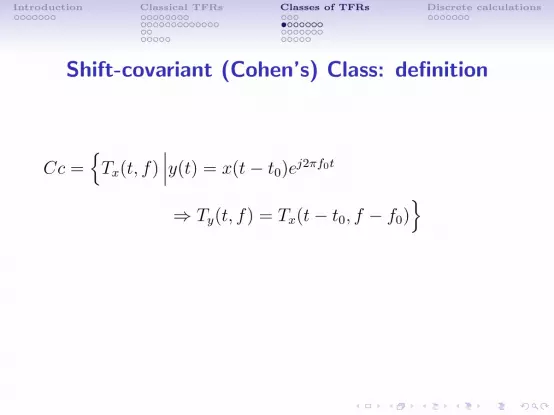
Shift-covariant (Cohen’s) Class: definition
Cc ={Tx(t, f)
∣∣∣y(t) = x(t− t0)ej2πf0t
⇒ Ty(t, f) = Tx(t− t0, f − f0)}

Introduction Classical TFRs Classes of TFRs Discrete calculations
Shift-covariant (Cohen’s) Class: definition
Cc ={Tx(t, f)
∣∣∣y(t) = x(t− t0)ej2πf0t
⇒ Ty(t, f) = Tx(t− t0, f − f0)}
Introduction Classical TFRs Classes of TFRs Discrete calculations
Shift-covariant (Cohen’s) Class: definition
Cc ={Tx(t, f)
∣∣∣y(t) = x(t− t0)ej2πf0t
⇒ Ty(t, f) = Tx(t− t0, f − f0)}

Introduction Classical TFRs Classes of TFRs Discrete calculations
Cc: Alternative Formulations
Any TFR within the Cohen’s class can be written in one of thefollowing equivalent “Normal Forms”
Cx(t, f ; Ψc)
=∫ ∫
φc(t− ς, τ)x(ς +
τ
2
)x∗(ς − τ
2
)e−j2πfτdςdτ
=∫ ∫
Φc(f − %, ζ)X(%+
ζ
2
)X∗(%− ζ
2
)e−j2πtζd%dζ
=∫ ∫
ψc(t− ς, f − %)Wx(ς, %)dςd%
=∫ ∫
Ψc(τ, ζ)Ax(τ, ζ)e−j2π(tζ−fτ)dτdζ
=∫ ∫
Υc(f − f1, f − f2)X(f1)X∗(f2)e−j2π(f1−f2)tdf1df2
where the kernels are interrelated by...

Introduction Classical TFRs Classes of TFRs Discrete calculations
Cc: Alternative Formulations
Any TFR within the Cohen’s class can be written in one of thefollowing equivalent “Normal Forms”
Cx(t, f ; Ψc) =∫ ∫
φc(t− ς, τ)x(ς +
τ
2
)x∗(ς − τ
2
)e−j2πfτdςdτ
=∫ ∫
Φc(f − %, ζ)X(%+
ζ
2
)X∗(%− ζ
2
)e−j2πtζd%dζ
=∫ ∫
ψc(t− ς, f − %)Wx(ς, %)dςd%
=∫ ∫
Ψc(τ, ζ)Ax(τ, ζ)e−j2π(tζ−fτ)dτdζ
=∫ ∫
Υc(f − f1, f − f2)X(f1)X∗(f2)e−j2π(f1−f2)tdf1df2
where the kernels are interrelated by...

Introduction Classical TFRs Classes of TFRs Discrete calculations
Cc: Alternative Formulations
φc(t, τ) =∫ ∫
Φc(f, ζ)e−j2π(fτ+tζ)dfdζ
=∫
Ψc(τ, ζ)e−j2πζtdζ
F←→ Φc(f, ζ)

Introduction Classical TFRs Classes of TFRs Discrete calculations
Cc: Alternative Formulations
φc(t, τ) =∫ ∫
Φc(f, ζ)e−j2π(fτ+tζ)dfdζ
=∫
Ψc(τ, ζ)e−j2πζtdζ
F←→ Φc(f, ζ)

Introduction Classical TFRs Classes of TFRs Discrete calculations
Cc: Alternative Formulations
φc(t, τ) =∫ ∫
Φc(f, ζ)e−j2π(fτ+tζ)dfdζ
=∫
Ψc(τ, ζ)e−j2πζtdζ
F←→ Φc(f, ζ)

Introduction Classical TFRs Classes of TFRs Discrete calculations
Cc: Alternative Formulations
ψc(t, f) =∫ ∫
Ψc(τ, ζ)e−j2π(tζ−fτ)dfdζ
=∫
Φc(f, ζ)e−j2πζtdζ
F←→ Ψc(τ, ζ)
and
Υc(f1, f2) = Φc
(f1 + f2
2, f2 − f1
)

Introduction Classical TFRs Classes of TFRs Discrete calculations
Cc: Alternative Formulations
ψc(t, f) =∫ ∫
Ψc(τ, ζ)e−j2π(tζ−fτ)dfdζ
=∫
Φc(f, ζ)e−j2πζtdζ
F←→ Ψc(τ, ζ)
and
Υc(f1, f2) = Φc
(f1 + f2
2, f2 − f1
)

Introduction Classical TFRs Classes of TFRs Discrete calculations
Cc: Alternative Formulations
ψc(t, f) =∫ ∫
Ψc(τ, ζ)e−j2π(tζ−fτ)dfdζ
=∫
Φc(f, ζ)e−j2πζtdζ
F←→ Ψc(τ, ζ)
and
Υc(f1, f2) = Φc
(f1 + f2
2, f2 − f1
)

Introduction Classical TFRs Classes of TFRs Discrete calculations
Cc: Alternative Formulations
ψc(t, f) =∫ ∫
Ψc(τ, ζ)e−j2π(tζ−fτ)dfdζ
=∫
Φc(f, ζ)e−j2πζtdζ
F←→ Ψc(τ, ζ)
and
Υc(f1, f2) = Φc
(f1 + f2
2, f2 − f1
)

Introduction Classical TFRs Classes of TFRs Discrete calculations
TRFs into the Cohen’s Class (1/3)

Introduction Classical TFRs Classes of TFRs Discrete calculations
TRFs into the Cohen’s Class (2/3)

Introduction Classical TFRs Classes of TFRs Discrete calculations
TRFs into the Cohen’s Class (3/3)

Introduction Classical TFRs Classes of TFRs Discrete calculations
Affine Class: definition
Ac ={Tx(t, f)
∣∣∣y(t) =√|a|x (a(t− t0))
⇒ Ty(t, f) = Tx(a(t− t0), fa
)}

Introduction Classical TFRs Classes of TFRs Discrete calculations
Affine Class: definition
Ac ={Tx(t, f)
∣∣∣y(t) =√|a|x (a(t− t0))
⇒ Ty(t, f) = Tx(a(t− t0), fa
)}

Introduction Classical TFRs Classes of TFRs Discrete calculations
Affine Class: definition
Ac ={Tx(t, f)
∣∣∣y(t) =√|a|x (a(t− t0))
⇒ Ty(t, f) = Tx(a(t− t0), fa
)}

Introduction Classical TFRs Classes of TFRs Discrete calculations
Ac: Alternative Formulations
Ax(t, f ; Ψa)
= |f |∫ ∫
φa(f(t− ς), fτ)x(ς +
τ
2
)x∗(ς − τ
2
)e−j2πfτdςdτ
=1|f |
∫ ∫Φa
(%
f,ζ
f
)X
(%+
ζ
2
)X∗(%− ζ
2
)e−j2πtζd%dζ
=∫ ∫
ψa
(f(t− ς),− %
f
)Wx(ς, %)dςd%
=∫ ∫
Ψa
(fτ,
ζ
f
)Ax(τ, ζ)e−j2π(tζ−fτ)dτdζ
=1|f |
∫ ∫Υa
(f1f,f2f
)X(f1)X∗(f2)e−j2π(f1−f2)tdf1df2
where the kernels are interrelated by...

Introduction Classical TFRs Classes of TFRs Discrete calculations
Ac: Alternative Formulations
Ax(t, f ; Ψa) = |f |∫ ∫
φa(f(t− ς), fτ)x(ς +
τ
2
)x∗(ς − τ
2
)e−j2πfτdςdτ
=1|f |
∫ ∫Φa
(%
f,ζ
f
)X
(%+
ζ
2
)X∗(%− ζ
2
)e−j2πtζd%dζ
=∫ ∫
ψa
(f(t− ς),− %
f
)Wx(ς, %)dςd%
=∫ ∫
Ψa
(fτ,
ζ
f
)Ax(τ, ζ)e−j2π(tζ−fτ)dτdζ
=1|f |
∫ ∫Υa
(f1f,f2f
)X(f1)X∗(f2)e−j2π(f1−f2)tdf1df2
where the kernels are interrelated by...

Introduction Classical TFRs Classes of TFRs Discrete calculations
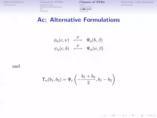
Ac: Alternative Formulations
φa(c, ν) F←→ Φa(b, β)
ψa(c, b)F←→ Ψa(ν, β)
and
Υa(b1, b2) = Φc
(−b1 + b2
2, b1 − b2
)

Introduction Classical TFRs Classes of TFRs Discrete calculations
Ac: Alternative Formulations
φa(c, ν) F←→ Φa(b, β)
ψa(c, b)F←→ Ψa(ν, β)
and
Υa(b1, b2) = Φc
(−b1 + b2
2, b1 − b2
)
Introduction Classical TFRs Classes of TFRs Discrete calculations
Ac: Alternative Formulations
φa(c, ν) F←→ Φa(b, β)
ψa(c, b)F←→ Ψa(ν, β)
and
Υa(b1, b2) = Φc
(−b1 + b2
2, b1 − b2
)
Introduction Classical TFRs Classes of TFRs Discrete calculations
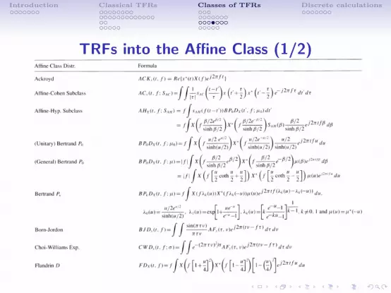
TRFs into the Affine Class (1/2)

Introduction Classical TFRs Classes of TFRs Discrete calculations
TRFs into the Affine Class (2/2)

Introduction Classical TFRs Classes of TFRs Discrete calculations
Affine-Cohen Subclass: definition
ACc ={Tx(t, f)
∣∣∣y(t) =√|a|x (a(t− t0)) ej2πf0t
⇒ Ty(t, f) = Tx(a(t− t0), f−f0
a
)}

Introduction Classical TFRs Classes of TFRs Discrete calculations
Affine-Cohen Subclass: definition
ACc ={Tx(t, f)
∣∣∣y(t) =√|a|x (a(t− t0)) ej2πf0t
⇒ Ty(t, f) = Tx(a(t− t0), f−f0
a
)}

Introduction Classical TFRs Classes of TFRs Discrete calculations
Affine-Cohen Subclass: definition
ACc ={Tx(t, f)
∣∣∣y(t) =√|a|x (a(t− t0)) ej2πf0t
⇒ Ty(t, f) = Tx(a(t− t0), f−f0
a
)}

Introduction Classical TFRs Classes of TFRs Discrete calculations
TRFs into the Affine-Cohen Subclass

Introduction Classical TFRs Classes of TFRs Discrete calculations
Hyperbolic Class: definition
Hc =
{Tx(t, f)
∣∣∣∣∣Y (f) = 1√|a|X(fa
)1√fej2πc ln(f/fr)
⇒ Ty(t, f) = Tx
(a(t− c
f
), fa
)}

Introduction Classical TFRs Classes of TFRs Discrete calculations
Hyperbolic Class: definition
Hc =
{Tx(t, f)
∣∣∣∣∣Y (f) = 1√|a|X(fa
)1√fej2πc ln(f/fr)
⇒ Ty(t, f) = Tx
(a(t− c
f
), fa
)}

Introduction Classical TFRs Classes of TFRs Discrete calculations
Hyperbolic Class: definition
Hc =
{Tx(t, f)
∣∣∣∣∣Y (f) = 1√|a|X(fa
)1√fej2πc ln(f/fr)
⇒ Ty(t, f) = Tx
(a(t− c
f
), fa
)}

Introduction Classical TFRs Classes of TFRs Discrete calculations
Affine-Hyperbolic Subclass: definition
AHc =
{Tx(t, f)
∣∣∣∣∣Y (f) = 1√|a|X(fa
)ej2πc ln(f/fr)ej2πft0
⇒ Ty(t, f) = Tx
(a(t− t0 − c
f
), fa
)}

Introduction Classical TFRs Classes of TFRs Discrete calculations
Affine-Hyperbolic Subclass: definition
AHc =
{Tx(t, f)
∣∣∣∣∣Y (f) = 1√|a|X(fa
)ej2πc ln(f/fr)ej2πft0
⇒ Ty(t, f) = Tx
(a(t− t0 − c
f
), fa
)}

Introduction Classical TFRs Classes of TFRs Discrete calculations
Affine-Hyperbolic Subclass: definition
AHc =
{Tx(t, f)
∣∣∣∣∣Y (f) = 1√|a|X(fa
)ej2πc ln(f/fr)ej2πft0
⇒ Ty(t, f) = Tx
(a(t− t0 − c
f
), fa
)}

Introduction Classical TFRs Classes of TFRs Discrete calculations
κth Power Class: definition
Pκc =
{Tx(t, f)
∣∣∣∣∣Y (f) = 1√|a|X(fa
)esgn(f)j2πc|(f/fr)|κ
⇒ Ty(t, f) = Tx
(a
(t− κ
fr
∣∣∣ ffr ∣∣∣κ−1), fa
)}

Introduction Classical TFRs Classes of TFRs Discrete calculations
κth Power Class: definition
Pκc =
{Tx(t, f)
∣∣∣∣∣Y (f) = 1√|a|X(fa
)esgn(f)j2πc|(f/fr)|κ
⇒ Ty(t, f) = Tx
(a
(t− κ
fr
∣∣∣ ffr ∣∣∣κ−1), fa
)}

Introduction Classical TFRs Classes of TFRs Discrete calculations
κth Power Class: definition
Pκc =
{Tx(t, f)
∣∣∣∣∣Y (f) = 1√|a|X(fa
)esgn(f)j2πc|(f/fr)|κ
⇒ Ty(t, f) = Tx
(a
(t− κ
fr
∣∣∣ ffr ∣∣∣κ−1), fa
)}

Introduction Classical TFRs Classes of TFRs Discrete calculations
κth Power Class: example
Let be
ξ(f) = sgn(f)|f |κ, κ 6= 0
andY (f) = X(f)e−j2πcξ(f/fr)
For a TFR in the κth power class we have
Pκy(t, f) = Pκx
(t− c κ
fr
∣∣∣∣ ffr∣∣∣∣κ−1
, f
)
= Pκx
(t− c d
dfξ(f/fr), f
)

Introduction Classical TFRs Classes of TFRs Discrete calculations
κth Power Class: example
Let be
ξ(f) = sgn(f)|f |κ, κ 6= 0
andY (f) = X(f)e−j2πcξ(f/fr)
For a TFR in the κth power class we have
Pκy(t, f) = Pκx
(t− c κ
fr
∣∣∣∣ ffr∣∣∣∣κ−1
, f
)
= Pκx
(t− c d
dfξ(f/fr), f
)

Introduction Classical TFRs Classes of TFRs Discrete calculations
κth Power Class: example
Let be
ξ(f) = sgn(f)|f |κ, κ 6= 0
andY (f) = X(f)e−j2πcξ(f/fr)
For a TFR in the κth power class we have
Pκy(t, f) = Pκx
(t− c κ
fr
∣∣∣∣ ffr∣∣∣∣κ−1
, f
)
= Pκx
(t− c d
dfξ(f/fr), f
)

Introduction Classical TFRs Classes of TFRs Discrete calculations
κth Power Class: example
Let be
ξ(f) = sgn(f)|f |κ, κ 6= 0
andY (f) = X(f)e−j2πcξ(f/fr)
For a TFR in the κth power class we have
Pκy(t, f) = Pκx
(t− c κ
fr
∣∣∣∣ ffr∣∣∣∣κ−1
, f
)
= Pκx
(t− c d
dfξ(f/fr), f
)

Introduction Classical TFRs Classes of TFRs Discrete calculations
κth Power Class: example
Let be
ξ(f) = sgn(f)|f |κ, κ 6= 0
andY (f) = X(f)e−j2πcξ(f/fr)
For a TFR in the κth power class we have
Pκy(t, f) = Pκx
(t− c κ
fr
∣∣∣∣ ffr∣∣∣∣κ−1
, f
)
= Pκx
(t− c d
dfξ(f/fr), f
)

Introduction Classical TFRs Classes of TFRs Discrete calculations
Classes and its Common Properties

Introduction Classical TFRs Classes of TFRs Discrete calculations
Outline
Introduction
Classical Time-Frequency RepresentationsShort-Time Fourier TransformsWigner DistributionAltes Q DistributionCross-Term Problems
Classes of TFRsClasses of TFRs with Common PropertiesShift-covariant ClassAffine ClassHyperbolic and kth Power Classes
Discrete calculations of TFRs

Introduction Classical TFRs Classes of TFRs Discrete calculations
Discrete calculations of TFRs
Sampling the signal...
...sampling the kernel...
... and defining discrete-timeand discrete-frequency distributions.
Introduction Classical TFRs Classes of TFRs Discrete calculations
Discrete calculations of TFRs
Sampling the signal...
...sampling the kernel...
... and defining discrete-timeand discrete-frequency distributions.

Introduction Classical TFRs Classes of TFRs Discrete calculations
Discrete calculations of TFRs
Sampling the signal...
...sampling the kernel...
... and defining discrete-timeand discrete-frequency distributions.
Introduction Classical TFRs Classes of TFRs Discrete calculations
Discrete calculations of TFRs
Sampling the signal...
...sampling the kernel...
... and defining discrete-timeand discrete-frequency distributions.

Introduction Classical TFRs Classes of TFRs Discrete calculations
Discrete-time Wigner Distribution
Wx(n, ejω) = 2
∑m
x(n+m)x∗(n−m)e−j2ωm

Introduction Classical TFRs Classes of TFRs Discrete calculations
Discrete-time Wigner Distribution
We know that for discrete signal x(n)
X(ejω) = X(ejω+k2π), k ∈ Z
However for the discrete-time WD we have the property
Wx(n, ejω) = Wx(n, ejω+kπ)
why...?

Introduction Classical TFRs Classes of TFRs Discrete calculations
Discrete-time Wigner Distribution
We know that for discrete signal x(n)
X(ejω) = X(ejω+k2π), k ∈ Z
However for the discrete-time WD we have the property
Wx(n, ejω) = Wx(n, ejω+kπ)
why...?

Introduction Classical TFRs Classes of TFRs Discrete calculations
Discrete-Time Wigner Distribution
Wx(n, ejω) = 2∑m
x(n+m)x∗(n−m)e−j2ωm
Now, to avoid the aliasing in the discrete-time WD we need
fs ≥ 4fmax

Introduction Classical TFRs Classes of TFRs Discrete calculations
General Discrete-Time TFRs
The general discrete-time time-frequency distribution ofCohen’s class is defined as
Cx(n, k) =M∑
m=−M
N∑`=−N
φ(`,m)x(`+n+m)x∗(`+n−m)e−j4πkm/L
...considering only the discrete frequencies up to 2πk/L, with Lthe DFT length.

Introduction Classical TFRs Classes of TFRs Discrete calculations
The Discrete-Time Choi-Williams TFR
φCW (n,m) =
{1
|m|αm e−σn2/4m2
, m 6= 0
δ(n), m = 0
with
αm =N∑
k=−N
1|m|
e−σn2/4m2

Introduction Classical TFRs Classes of TFRs Discrete calculations
The Discrete-Time Choi-Williams TFR
φCW (n,m) =
{1
|m|αm e−σn2/4m2
, m 6= 0
δ(n), m = 0
with
αm =N∑
k=−N
1|m|
e−σn2/4m2

Introduction Classical TFRs Classes of TFRs Discrete calculations
The Discrete-Time Choi-Williams TFR
With the normalization∑
n φ(n,m) = 1 the followinginteresting properties are preserved
∑n
CWx(n, k) = |X(k)|2
and ∑k
CWx(n, k) = |x(n)|2

Introduction Classical TFRs Classes of TFRs Discrete calculations
Bibliography
[1] A. Mertins, Signal Analysis: Wavelets, Filter Banks,Time-Frequency Transforms and Applications, John Wiley &Sons, 1999.
[2] R. Allen, D. Mills, Signal Analysis: Time, Frequency, Scale andStructure, IEEE Press, John Wiley & Sons, 2004.
[3] G. Boudreaux-Bartels, Mixed Time-Frequency SignalTransformations, Chapter 12 in: Poularikas A. (Editor), TheTransforms and Applications Handbook, CRC Press, 2000.
[4] J. Jeong and W. J. Williams, “Alias-free generalizeddiscrete-time time-frequency distributions,” IEEE Trans. SignalProcessing, vol. 40, pp. 2757-2765, Nov. 1992.
[5] L. Cohen, “Time-frequency distributions – A review,” Proc.IEEE, vol. 77, pp. 941-981, July 1989.