Embed Size (px)
Citation preview

The Mathematics
of Foam
Christopher James William Breward
St Anne’s College
University of Oxford
A thesis submitted for the degree of
Doctor of Philosophy
June 1999

Contents
1 Introduction 1
1.1 What is a foam? . . . . . . . . . . . . . . . . . . . . . . . . . . . . . . . . 1
1.2 How do foams form? . . . . . . . . . . . . . . . . . . . . . . . . . . . . . . 5
1.3 Why does a foam persist after it has been formed? . . . . . . . . . . . . . . 5
1.3.1 Surfactants . . . . . . . . . . . . . . . . . . . . . . . . . . . . . . . 5
1.3.2 How does a surface tension gradient affect a liquid flow? . . . . . . 6
1.3.3 Volatile Components . . . . . . . . . . . . . . . . . . . . . . . . . . 7
1.4 What happens to lamellae when they become thin? . . . . . . . . . . . . . 7
1.5 How does a lamella rupture? . . . . . . . . . . . . . . . . . . . . . . . . . . 7
1.6 How are foams destroyed in industrial situations where they are not wanted? 8
1.7 Background material . . . . . . . . . . . . . . . . . . . . . . . . . . . . . . 8
1.8 Thesis plan . . . . . . . . . . . . . . . . . . . . . . . . . . . . . . . . . . . 12
1.9 Statement of Originality . . . . . . . . . . . . . . . . . . . . . . . . . . . . 13
2 Modelling of liquids, surfactants and volatile systems 14
2.1 Liquid modelling . . . . . . . . . . . . . . . . . . . . . . . . . . . . . . . . 15
2.1.1 Field Equations . . . . . . . . . . . . . . . . . . . . . . . . . . . . . 15
2.1.2 Boundary conditions . . . . . . . . . . . . . . . . . . . . . . . . . . 15
2.2 Surfactants . . . . . . . . . . . . . . . . . . . . . . . . . . . . . . . . . . . 16
2.2.1 Effect of surfactant on the surface tension . . . . . . . . . . . . . . 18
2.3 Volatile and Inert systems . . . . . . . . . . . . . . . . . . . . . . . . . . . 19
2.3.1 Volatile component at the free surface . . . . . . . . . . . . . . . . 19
2.3.2 Model for evaporation . . . . . . . . . . . . . . . . . . . . . . . . . 20
2.4 Summary . . . . . . . . . . . . . . . . . . . . . . . . . . . . . . . . . . . . 20
3 Modelling expanding free surfaces 22
3.1 Introduction . . . . . . . . . . . . . . . . . . . . . . . . . . . . . . . . . . . 22
3.2 The overflowing cylinder . . . . . . . . . . . . . . . . . . . . . . . . . . . . 22
3.3 Previous work . . . . . . . . . . . . . . . . . . . . . . . . . . . . . . . . . . 24
i

3.3.1 Experimental observations . . . . . . . . . . . . . . . . . . . . . . . 25
3.3.2 Plan . . . . . . . . . . . . . . . . . . . . . . . . . . . . . . . . . . . 31
3.4 Model formulation: velocity distribution . . . . . . . . . . . . . . . . . . . 31
3.4.1 Typical non-dimensional parameter sizes based on flow at depth . . 33
3.5 Model formulation: surfactant distribution . . . . . . . . . . . . . . . . . . 34
3.5.1 Linearisation . . . . . . . . . . . . . . . . . . . . . . . . . . . . . . 36
3.5.2 Nondimensional parameter sizes based on flow at depth . . . . . . . 37
3.6 Outer (Inviscid) Problem . . . . . . . . . . . . . . . . . . . . . . . . . . . . 37
3.6.1 Inviscid solution . . . . . . . . . . . . . . . . . . . . . . . . . . . . . 38
3.7 Outer (surfactant) Problem . . . . . . . . . . . . . . . . . . . . . . . . . . 42
3.7.1 Solution to the problem in the limit Ma→ 0 and S →∞ . . . . . . 42
3.8 Boundary layers at the free surface . . . . . . . . . . . . . . . . . . . . . . 42
3.8.1 The hydrodynamic boundary layer . . . . . . . . . . . . . . . . . . 44
3.8.2 The diffusion boundary layer . . . . . . . . . . . . . . . . . . . . . . 45
3.8.3 Coupling between the hydrodynamic and diffusive problems . . . . 45
3.9 Series solutions to both the liquid and surfactant problems . . . . . . . . . 47
3.9.1 The Solution for C∗ . . . . . . . . . . . . . . . . . . . . . . . . . . . 48
3.9.2 Lowest order liquid problem and solution . . . . . . . . . . . . . . . 49
3.9.3 Problem and solution for C2 . . . . . . . . . . . . . . . . . . . . . . 52
3.10 The lack of closure . . . . . . . . . . . . . . . . . . . . . . . . . . . . . . . 53
3.10.1 Termination of the series . . . . . . . . . . . . . . . . . . . . . . . . 54
3.10.2 Neglected physical effects . . . . . . . . . . . . . . . . . . . . . . . . 56
3.10.3 Edge Effects . . . . . . . . . . . . . . . . . . . . . . . . . . . . . . . 58
3.11 Conclusions . . . . . . . . . . . . . . . . . . . . . . . . . . . . . . . . . . . 58
4 Models for Marangoni flows in thin films with two free surfaces 61
4.1 Introduction . . . . . . . . . . . . . . . . . . . . . . . . . . . . . . . . . . . 61
4.1.1 Thin films with two free boundaries . . . . . . . . . . . . . . . . . . 61
4.1.2 Films on substrates . . . . . . . . . . . . . . . . . . . . . . . . . . . 62
4.1.3 Plan . . . . . . . . . . . . . . . . . . . . . . . . . . . . . . . . . . . 63
4.2 Thin film equations for the liquid . . . . . . . . . . . . . . . . . . . . . . . 63
4.3 Reduction to thin film equations . . . . . . . . . . . . . . . . . . . . . . . . 67
4.3.1 Distinguished Limits: Three forces balancing . . . . . . . . . . . . . 67
4.3.1.1 Viscous, capillary and Marangoni effects . . . . . . . . . . 67
4.3.1.2 Capillary, Marangoni and lubrication effects . . . . . . . . 69
4.3.2 Intermediate regimes where two forces balance . . . . . . . . . . . . 69
4.3.2.1 Capillary and Marangoni . . . . . . . . . . . . . . . . . . 69
ii

4.3.2.2 Capillary and viscous effects . . . . . . . . . . . . . . . . . 70
4.3.2.3 Marangoni and viscous effects . . . . . . . . . . . . . . . . 70
4.3.2.4 Marangoni and lubrication effects . . . . . . . . . . . . . . 71
4.3.3 Intermediate regimes where one force dominates . . . . . . . . . . . 71
4.3.3.1 Capillary effects . . . . . . . . . . . . . . . . . . . . . . . 71
4.3.3.2 Viscous effects . . . . . . . . . . . . . . . . . . . . . . . . 71
4.3.3.3 Marangoni effects . . . . . . . . . . . . . . . . . . . . . . . 72
4.3.4 Summary . . . . . . . . . . . . . . . . . . . . . . . . . . . . . . . . 73
4.4 The effects of gravity, pressure drops across the film, disjoining pressure,
and surface viscosity . . . . . . . . . . . . . . . . . . . . . . . . . . . . . . 73
4.4.1 Gravity . . . . . . . . . . . . . . . . . . . . . . . . . . . . . . . . . 76
4.4.2 Pressure drops across the film . . . . . . . . . . . . . . . . . . . . . 76
4.4.3 Van der Waals forces and disjoining pressure . . . . . . . . . . . . . 77
4.4.4 Closure of the models . . . . . . . . . . . . . . . . . . . . . . . . . . 77
4.5 Thin film equations: presence of a surfactant . . . . . . . . . . . . . . . . . 78
4.5.1 Distinguished Limits: three mechanisms balancing . . . . . . . . . . 80
4.5.1.1 Longitudinal diffusion, bulk convection and surface con-
vection . . . . . . . . . . . . . . . . . . . . . . . . . . . . 80
4.5.1.2 Diffusion across the film, bulk convection and surface con-
vection . . . . . . . . . . . . . . . . . . . . . . . . . . . . 81
4.5.2 Intermediate Regimes: Two mechanisms balancing . . . . . . . . . 82
4.5.2.1 Bulk convection and surface convection . . . . . . . . . . . 82
4.5.2.2 Diffusion across the film and bulk convection . . . . . . . 82
4.5.2.3 Longitudinal diffusion and surface convection . . . . . . . 82
4.5.2.4 Diffusion across the film and surface convection . . . . . . 82
4.5.3 Regimes where one mechanism dominates . . . . . . . . . . . . . . 83
4.5.3.1 Surface convection . . . . . . . . . . . . . . . . . . . . . . 83
4.5.3.2 Bulk convection . . . . . . . . . . . . . . . . . . . . . . . . 83
4.5.3.3 Longitudinal diffusion . . . . . . . . . . . . . . . . . . . . 83
4.5.3.4 Convection dominated flows . . . . . . . . . . . . . . . . . 84
4.5.4 Summary . . . . . . . . . . . . . . . . . . . . . . . . . . . . . . . . 85
4.5.5 The no-slip condition . . . . . . . . . . . . . . . . . . . . . . . . . . 85
4.5.6 Insoluble surfactants . . . . . . . . . . . . . . . . . . . . . . . . . . 85
4.6 Thin film equations: presence of a miscible, volatile component . . . . . . . 88
4.6.1 Distinguished limits: three mechanisms balancing . . . . . . . . . . 89
4.6.1.1 Convection, longitudinal diffusion and evaporation . . . . 89
4.6.1.2 Convection, diffusion across the film and evaporation . . . 90
iii
4.6.2 Intermediate regimes where two mechanisms balance . . . . . . . . 90
4.6.2.1 Convection and longitudinal diffusion . . . . . . . . . . . . 90
4.6.2.2 Convection and evaporation . . . . . . . . . . . . . . . . . 91
4.6.2.3 Convection and diffusion across the film . . . . . . . . . . 91
4.6.2.4 Convection and diffusion across the film (and evaporation) 91
4.6.3 Regimes where one mechanism is dominant . . . . . . . . . . . . . . 91
4.6.3.1 Diffusion . . . . . . . . . . . . . . . . . . . . . . . . . . . 91
4.6.3.2 Convection (well-mixed) . . . . . . . . . . . . . . . . . . . 92
4.6.3.3 Convection dominated flow . . . . . . . . . . . . . . . . . 92
4.6.3.4 Evaporation . . . . . . . . . . . . . . . . . . . . . . . . . . 92
4.6.4 Summary . . . . . . . . . . . . . . . . . . . . . . . . . . . . . . . . 93
4.7 Mathematical Structure of a typical coupled problem . . . . . . . . . . . . 93
4.8 Conclusion . . . . . . . . . . . . . . . . . . . . . . . . . . . . . . . . . . . . 96
5 Foam films 99
5.1 Introduction . . . . . . . . . . . . . . . . . . . . . . . . . . . . . . . . . . . 99
5.1.1 Relevant parameter sizes . . . . . . . . . . . . . . . . . . . . . . . . 101
5.1.2 Plan . . . . . . . . . . . . . . . . . . . . . . . . . . . . . . . . . . . 102
5.2 Evolution of a thin aqueous film in the absence of surfactant . . . . . . . . 103
5.2.1 Introduction and modelling ideas . . . . . . . . . . . . . . . . . . . 103
5.2.2 Model for a film acting under viscosity and capillarity . . . . . . . . 104
5.2.3 Lengthscale of the transition region and velocity scalings . . . . . . 105
5.2.4 Transition region . . . . . . . . . . . . . . . . . . . . . . . . . . . . 106
5.2.5 Lamella model . . . . . . . . . . . . . . . . . . . . . . . . . . . . . 107
5.2.6 Implications . . . . . . . . . . . . . . . . . . . . . . . . . . . . . . . 109
5.3 Evolution of films stabilised by a well-mixed soluble surfactant . . . . . . . 109
5.3.1 Selection of velocity scale . . . . . . . . . . . . . . . . . . . . . . . . 110
5.3.1.1 Parameter sizes and plan for the rest of this section . . . . 111
5.3.2 Plateau border . . . . . . . . . . . . . . . . . . . . . . . . . . . . . 112
5.3.3 Lamella model . . . . . . . . . . . . . . . . . . . . . . . . . . . . . 112
5.3.4 Transition region . . . . . . . . . . . . . . . . . . . . . . . . . . . . 114
5.3.4.1 Asymptotic behaviour of solutions at ±∞ . . . . . . . . . 115
5.3.5 Summary . . . . . . . . . . . . . . . . . . . . . . . . . . . . . . . . 117
5.3.6 Results and discussion . . . . . . . . . . . . . . . . . . . . . . . . . 118
5.3.6.1 Unexpected results . . . . . . . . . . . . . . . . . . . . . . 127
5.3.7 Including the ‘lubrication’ term . . . . . . . . . . . . . . . . . . . . 133
5.3.7.1 Behaviour as ξ → ±∞ . . . . . . . . . . . . . . . . . . . . 133
iv

5.3.7.2 Surface and centre-line velocities as ξ →∞ . . . . . . . . 134
5.3.7.3 Summary . . . . . . . . . . . . . . . . . . . . . . . . . . . 135
5.3.7.4 Results and discussion . . . . . . . . . . . . . . . . . . . . 136
5.3.8 Conclusions . . . . . . . . . . . . . . . . . . . . . . . . . . . . . . . 141
5.4 Example: evolution of a thin film stabilised by CTAB . . . . . . . . . . . . 142
5.4.1 Plateau Border . . . . . . . . . . . . . . . . . . . . . . . . . . . . . 142
5.4.2 Lamella . . . . . . . . . . . . . . . . . . . . . . . . . . . . . . . . . 142
5.4.3 Transition region . . . . . . . . . . . . . . . . . . . . . . . . . . . . 143
5.4.4 Implications . . . . . . . . . . . . . . . . . . . . . . . . . . . . . . . 144
5.5 Example: evolution of films stabilised by insoluble surfactants . . . . . . . 145
5.5.1 Plateau border . . . . . . . . . . . . . . . . . . . . . . . . . . . . . 146
5.5.2 Lamella . . . . . . . . . . . . . . . . . . . . . . . . . . . . . . . . . 146
5.5.3 Transition region . . . . . . . . . . . . . . . . . . . . . . . . . . . . 147
5.5.4 Asymptotics of the transition region . . . . . . . . . . . . . . . . . 147
5.5.5 Solution . . . . . . . . . . . . . . . . . . . . . . . . . . . . . . . . . 148
5.6 Preliminary model: film stabilised by a well-mixed volatile component . . . 148
5.6.1 Plateau border . . . . . . . . . . . . . . . . . . . . . . . . . . . . . 150
5.6.2 Lamella model . . . . . . . . . . . . . . . . . . . . . . . . . . . . . 150
5.6.3 Transition region . . . . . . . . . . . . . . . . . . . . . . . . . . . . 151
5.6.4 Implications . . . . . . . . . . . . . . . . . . . . . . . . . . . . . . . 152
5.7 Films stabilised by the presence of surface viscosity . . . . . . . . . . . . . 152
5.7.1 Transition region . . . . . . . . . . . . . . . . . . . . . . . . . . . . 153
5.7.2 Lamella model . . . . . . . . . . . . . . . . . . . . . . . . . . . . . 154
5.8 Conclusions . . . . . . . . . . . . . . . . . . . . . . . . . . . . . . . . . . . 156
6 Plateau border flow, macroscopic models and foam destruction 159
6.1 Introduction . . . . . . . . . . . . . . . . . . . . . . . . . . . . . . . . . . . 159
6.2 Plateau border flow . . . . . . . . . . . . . . . . . . . . . . . . . . . . . . . 159
6.2.1 An ad-hoc model for drainage of a Plateau border incorporating
zero shear on the walls . . . . . . . . . . . . . . . . . . . . . . . . . 161
6.2.2 Application to foam build-up . . . . . . . . . . . . . . . . . . . . . 162
6.2.2.1 Experimental set up . . . . . . . . . . . . . . . . . . . . . 162
6.2.2.2 Foam Height . . . . . . . . . . . . . . . . . . . . . . . . . 163
6.2.2.3 Homogenisation . . . . . . . . . . . . . . . . . . . . . . . . 163
6.3 Foam destruction . . . . . . . . . . . . . . . . . . . . . . . . . . . . . . . . 167
6.3.1 First experimental set up . . . . . . . . . . . . . . . . . . . . . . . . 167
6.3.1.1 Homogenised model . . . . . . . . . . . . . . . . . . . . . 167
v
6.3.2 Second experimental set up . . . . . . . . . . . . . . . . . . . . . . 170
6.3.2.1 Microscopic model . . . . . . . . . . . . . . . . . . . . . . 170
6.4 Short-comings of the models . . . . . . . . . . . . . . . . . . . . . . . . . . 172
7 Conclusion 173
7.1 Review of thesis . . . . . . . . . . . . . . . . . . . . . . . . . . . . . . . . . 173
7.2 Future work . . . . . . . . . . . . . . . . . . . . . . . . . . . . . . . . . . . 175
7.3 Experiments that would provide extra insight into foam modelling . . . . . 177
7.4 Discussion . . . . . . . . . . . . . . . . . . . . . . . . . . . . . . . . . . . . 178
Bibliography 179
vi

List of Figures
1.1 Schematic of (a) a wet foam and (b) a dry foam. . . . . . . . . . . . . . . . 2
1.2 High speed photograph of a foam (courtesy of Kui-Hua Sun, Engineering
Department, University of Oxford). . . . . . . . . . . . . . . . . . . . . . . 3
1.3 Schematic of liquid within a foam. . . . . . . . . . . . . . . . . . . . . . . . 4
1.4 Close up of a lamella between two Plateau borders. . . . . . . . . . . . . . 4
1.5 Surfactant molecules (a) forming a micelle and (b) at a free surface. . . . . 6
1.6 The Kelvin Cell (courtesy of Andy Kraynik). . . . . . . . . . . . . . . . . . 10
1.7 A random foam structure (courtesy of Andy Kraynik). . . . . . . . . . . . 10
1.8 Schematic of a layer of bubbles moving over the top of another layer. . . . 11
1.9 Schematic of experiment to study a bubble train moving through a cavity. 12
3.1 The overflowing cylinder. . . . . . . . . . . . . . . . . . . . . . . . . . . . . 23
3.2 Close-up of the overflowing cylinder. . . . . . . . . . . . . . . . . . . . . . 24
3.3 Display formula for CTAB. . . . . . . . . . . . . . . . . . . . . . . . . . . . 25
3.4 Surface speed measurements (Vr measured in mm s−1) against distance (r
measured in mm), for a number of bulk concentrations. . . . . . . . . . . . 25
3.5 Surface speed measurements (Vr measured in mm s−1) against distance (r
measured in mm), for pure water. . . . . . . . . . . . . . . . . . . . . . . . 26
3.6 Horizontal speed (Vr in mm s−1), for a number of depths (h in mm), at
r = 6mm (circles), r = 12mm (triangles) and r = 20mm (upside down
triangles). . . . . . . . . . . . . . . . . . . . . . . . . . . . . . . . . . . . . 27
3.7 The Langmuir isotherm. . . . . . . . . . . . . . . . . . . . . . . . . . . . . 27
3.8 Variation of surface tension (σ in mN m−1) with distance across the cylinder
(r in mm), for various bulk concentrations: (a) 0.1, (b) 0.17, (c) 0.25, (d)
0.31, (e) 0.35, (f) 0.46, (g) 0.51, (h) 0.58, (i) 0.68, (j) 0.81 mol m−3. . . . . 28
3.9 Variation of surface tension (σ0 in mN m−1) with bulk concentration (C in
mol m−3) measured under static conditions. . . . . . . . . . . . . . . . . . 29
vii

3.10 Variation of surface concentration (Γ in mol m−2) with distance across the
cylinder (r in mm), for various bulk concentrations: 0.1 mol m−3 (black
triangles), 0.31 mol m−3 (open circles), 0.58 mol m−3 (black diamonds),
0.81 mol m−3 (open triangles) and 1.73 mol m−3 (black squares). . . . . . . 30
3.11 Langmuir isotherm showing Υ∗, Γ∗ and the variation of Γ and C at the
surface (in red). . . . . . . . . . . . . . . . . . . . . . . . . . . . . . . . . . 35
3.12 Plot showing the inviscid velocity field. . . . . . . . . . . . . . . . . . . . . 40
3.13 Graph showing the solution, (??), for u (in black), compared with the
expansion (??), for u (in red). . . . . . . . . . . . . . . . . . . . . . . . . . 41
3.14 Schematic of the boundary layer structure: g(r) = V 2lruout(lr)u′out(lr). . . 46
3.15 Graph showing C∗(ζ) versus depth ζ for Υ = 0.3, 0.4, 0.5 and 0.6. . . . . . 49
3.16 The solution f0 (black) and f ′0 (red) to (??)–(??), for Υ = 0.4, λ = 4.57. . 50
3.17 Graph showing how f ′′(0) varies with Υ. λ = 4.57. . . . . . . . . . . . . . 51
3.18 Flowchart showing transfer of information. . . . . . . . . . . . . . . . . . . 51
4.1 A thin film of liquid between two free surfaces. . . . . . . . . . . . . . . . . 64
4.2 Schematic showing where the models lie in U , T space. The red blocks show
the distinguished limits, the blue blocks show the intermediate regimes
where two mechanisms balance, and the green blocks show the limits in
which one mechanism dominates. . . . . . . . . . . . . . . . . . . . . . . . 74
4.3 Table showing regimes. . . . . . . . . . . . . . . . . . . . . . . . . . . . . . 75
4.4 Schematic showing where the models lie in U , Hp space. The red blocks
show the distinguished limits, the blue blocks show the intermediate regimes
where two mechanisms balance, and the green blocks show the limits in
which one mechanism dominates. . . . . . . . . . . . . . . . . . . . . . . . 86
4.5 Table showing regimes. . . . . . . . . . . . . . . . . . . . . . . . . . . . . . 87
4.6 Schematic showing where the models lie in U , E space. The red blocks show
the distinguished limits, the blue blocks show the intermediate regimes in
which two mechanisms balance, and the green blocks show the regimes in
which one force dominates. . . . . . . . . . . . . . . . . . . . . . . . . . . . 94
4.7 Table showing regimes. . . . . . . . . . . . . . . . . . . . . . . . . . . . . . 95
5.1 Schwartz and Princen’s liquid regime. . . . . . . . . . . . . . . . . . . . . . 100
5.2 Barigou and Davidson’s liquid regime. . . . . . . . . . . . . . . . . . . . . 100
5.3 The ‘outer’ picture. . . . . . . . . . . . . . . . . . . . . . . . . . . . . . . . 103
5.4 The ‘inner’ picture. . . . . . . . . . . . . . . . . . . . . . . . . . . . . . . . 104
5.5 Transition region shape. . . . . . . . . . . . . . . . . . . . . . . . . . . . . 107
5.6 Transition region pressure profile. . . . . . . . . . . . . . . . . . . . . . . . 108
viii

5.7 Flowchart showing information routes. . . . . . . . . . . . . . . . . . . . . 119
5.8 Results for thickness and concentration in a monotonic solution. . . . . . . 120
5.9 Results for thickness and concentration in a dimpled solution. . . . . . . . 121
5.10 Surface convection (blue), bulk convection (green) and bulk diffusion (red)
for a monotonic solution. . . . . . . . . . . . . . . . . . . . . . . . . . . . . 122
5.11 Surface convection (blue), bulk convection (green) and bulk diffusion (red)
for a nonmonotonic solution. . . . . . . . . . . . . . . . . . . . . . . . . . . 122
5.12 Pressure in a monotonic solution (red) and a dimpled solution (blue). . . . 123
5.13 Barigou and Davidson’s rejected transition region. . . . . . . . . . . . . . . 124
5.14 Graph showing Q as a function of h0 for P = 0.5, T = 0.5, CI = 0.1. . . . 125
5.15 Transition region thickness for various values of h0, with P = 0.5, T = 0.5,
CI = 0.1. . . . . . . . . . . . . . . . . . . . . . . . . . . . . . . . . . . . . . 125
5.16 Concentration in the transition region for various values of h0, with P =
0.5, T = 0.5, CI = 0.1 . . . . . . . . . . . . . . . . . . . . . . . . . . . . . 126
5.17 Graph showing lamella thickness versus time for P = 0.5, T = 0.5, and
CI = 0.1. . . . . . . . . . . . . . . . . . . . . . . . . . . . . . . . . . . . . . 127
5.18 Graph showing Q against h0 for CI = 0.5, P = 5, and T = 5. . . . . . . . . 128
5.19 Graph showing how the function F varies with T ∗ . . . . . . . . . . . . . 131
5.20 Schematic showing how the thickness of a lamella changes with time. The
upper part of the curve was calculated for CI = 0.5, P = 5, T = 5. . . . . . 132
5.21 Velocity field for a solution where K > 1. . . . . . . . . . . . . . . . . . . . 136
5.22 Velocity field for a solution where K < 1. . . . . . . . . . . . . . . . . . . . 137
5.23 Graphs showing surface velocities and centreline velocities in the cases CI <
P/(2 + P) (figures (a) and (c)) and CI > P/(2 + P) (figures (b) and (d)),
for β = 0 (black), 0.2 (red), 0.4 (green), 0.6 (blue), 0.8 (purple), and 1.0
(cyan). . . . . . . . . . . . . . . . . . . . . . . . . . . . . . . . . . . . . . . 138
5.24 Graph showing Q as a function of h0 for P = 0.5, T = 0.5, CI = 0.1, and
β = 1. . . . . . . . . . . . . . . . . . . . . . . . . . . . . . . . . . . . . . . 140
5.25 Graph showing lamella thickness with time for P = 0.5, T = 0.5, CI = 0.1
and β = 1.0. . . . . . . . . . . . . . . . . . . . . . . . . . . . . . . . . . . . 140
5.26 Graph showing the variation of Q∗ with h0 for T = 1, P∗ = 0.1 and CI = 0.1144
5.27 Graph showing the variation of Q with h0 when T = 0.5 and ΓI = 0.1 . . . 149
5.28 Transition region shape . . . . . . . . . . . . . . . . . . . . . . . . . . . . . 154
6.1 A Plateau border aligned with its centreline in the direction of gravity. . . 161
6.2 Diagram showing the foam rig. . . . . . . . . . . . . . . . . . . . . . . . . 163
ix
6.3 Antifoam production: the top layer of foam was removed and allowed to
break down. The solution was added to the foam and it dramatically
reduced its height . . . . . . . . . . . . . . . . . . . . . . . . . . . . . . . . 168
6.4 Graph showing how the total average surfactant concentration varied in
the rig. The height is in metres and the concentration is in moles per cubic
metre. . . . . . . . . . . . . . . . . . . . . . . . . . . . . . . . . . . . . . . 169
6.5 Schematic showing the hot gauze restricting the growth of a foam. . . . . . 170
6.6 Close-up of lamella at the surface of the foam, with the hot gauze above . . 172
7.1 The jet experiment. . . . . . . . . . . . . . . . . . . . . . . . . . . . . . . . 175
x

Acknowledgements
I should like to thank a number of important people who have assisted me
in many areas during my research time at Oxford. I’ll start with my official
supervisors: John Ockendon, and Richard Darton. They have both been
extremely useful: John has continued to ensure that I perform to the best of
my mathematical ability, while Richard has always endeavoured to ‘keep me
on the straight and narrow’. Peter Howell, while not an official supervisor,
has been an invaluable and irreplaceable source of ideas. He has ensured that
I remained focussed on the task in hand, no matter how often I attempted to
stray from the path.
We have been in close collaboration with Colin Bain and Samantha Manning-
Benson, from the Physical and Theoretical Chemistry Laboratory, who have
provided us with insight into the behaviour of surfactants at surfaces, and a
wealth of experimental data from the overflowing cylinder.
I should also like to thank Kui-Hua Sun from Engineering Department, for
the high speed camera picture of a foam, Andy Kraynik for the pictures of the
Kelvin cell and the random foam and Warrick Cooke, from OCIAM, for devel-
oping some mathematica code to enable the plotting of vector fields between
two free surfaces.
There are numerous other people have made my DPhil time pleasant: My
family; the old and not-so-old DH9 crew Keith, Mark, Dave, John and Jim;
the rest of OCIAM; the members of St Anne’s, especially Ele, Jason, Clare and
Dr Hilary Priestley; and the members of my air cadet unit, 2267 (Lechlade)
Detached Flight.
Finally I should like to finish by thanking Dr Mary Kearsley. Without her
unending stories, I would never have remembered a whole host of mathematical
concepts, including my favourite vector identity: curl curl equals grad div
minus del squared.

The Mathematics
of Foam
Christopher James William Breward
St Anne’s CollegeUniversity of Oxford
A thesis submitted for the degree ofDoctor of Philosophy
June 1999
The aim of this thesis is to derive and solve mathematical models for the flow of liquid
in a foam. A primary concern is to investigate how so-called “Marangoni stresses” (i.e.
surface tension gradients), generated for example by the presence of a surfactant, act to
stabilise a foam. We aim to provide the key microscopic components for future foam
modelling.
We begin by describing in detail the influence of surface tension gradients on a general
liquid flow, and various physical mechanisms which can give rise to such gradients. We
apply the models thus devised to an experimental configuration designed to investigate
Marangoni effects.
Next we turn our attention to the flow in the thin liquid films (“lamellae”) which make
up a foam. Our methodology is to simplify the field equations (e.g. the Navier-Stokes
equations for the liquid) and free surface conditions using systematic asymptotic methods.
The models so derived explain the “stiffening” effect of surfactants at free surfaces, which
extends considerably the lifetime of a foam.
Finally, we look at the macroscopic behaviour of foam using an ad-hoc averaging of the
thin film models.

Chapter 1
Introduction
Liquid foams occur in a wide variety of contexts. In everyday life, they form the froth
in a washing-up bowl, and the head on a pint of beer. Practically, they are important,
for example, in dampening explosions, collecting radioactive dust, dyeing materials and
crop spraying. In all these applications, the ability of a foam to spread a small amount of
liquid over a wide area is crucial. Foams are also used in the mineral recovery industry
(the largest industry in the world). Here, it is the foam’s ability to preferentially select
one mineral over another which is important. This process has also been used to separate
proteins. However, the presence of a foam is not always beneficial. For example, in the
brewing industry, the presence of a foam during beer production is undesirable because
it both reduces vessel capacity and lessens the foam potential of the finished product
(see Bamforth [4]). Also, the presence of unwanted foam in a distillation column can
cause substantial problems such as loss of throughput or deterioration in product quality
throught loss of separation efficiency. In any case, it is desirable to understand the bulk
properties of a foam and how they depend on those of its constituents.
1.1 What is a foam?
A foam is a gas-liquid mixture in which the volume fraction of the liquid phase is small.
Foams are broadly divided into ‘wet’ and ‘dry’, depending on the proportion of liquid
contained in them. In a wet foam (where the liquid volume fraction is typically between
10% and 20%) the bubbles are approximately spherical, while in a dry foam (where the
volume fraction of liquid is less than 10%), the bubbles are more polyhedral in shape as
in Figure 1.1. In a dry foam (as shown in a high speed photograph in Figure 1.2), the
thin films forming the faces of the roughly polyhedral bubbles are called lamellae and the
“tubes” of liquid at the junctions of these films are called Plateau borders, named after
1

(a) (b)
Figure 1.1: Schematic of (a) a wet foam and (b) a dry foam.
Plateau, following his paper [66] discussing the angle at which three soap films meet. The
vertices where typically four Plateau borders meet are called nodes.
We warn that pictures of foam are often misleading, since they are two-dimensional repre-
sentations of three-dimensional structures. For example, in the photograph in Figure 1.2,
the dark lines are Plateau borders, the lamellae span these dark lines and the nodes are
the junctions of these lines. In the two-dimensional schematics of Figure 1.1, however, the
lines represent the lamellae and the junctions of the lines represent Plateau borders; we
cannot easily depict the nodes in these two dimensional representations. We show three
dimensional schematics of the liquid distribution within a dry foam in Figures 1.3 and
1.4.
2

Figure 1.2: High speed photograph of a foam (courtesy of Kui-Hua Sun, EngineeringDepartment, University of Oxford).
3

LamellaNode
Plateau Border
Figure 1.3: Schematic of liquid within a foam.
LamellaPlateau Border
Figure 1.4: Close up of a lamella between two Plateau borders.
4
1.2 How do foams form?
Foams are formed when a gas and liquid are mixed. There are many ways in which this
can occur, including:
• when a gas passes through a liquid, such as in a distillation column;
• when a gas and liquid are mixed and the gaseous phase is entrained, for example,
when generating bubble bath foam;
• when a gas is released from solution due to a change in pressure, such as upon
opening a bottle of fizzy pop.
Once a foam has been formed, its lifetime is determined by the flow of liquid, and the
subsequent distribution of the various chemical components, through the microstructure.
In general, a foam starts wet and becomes dryer as the liquid drains out of it. For
some systems, this process proceeds until a stable volume fraction is reached after which
the foam can last virtually indefinitely (due to intermolecular interactions). In others,
the foam has a finite lifetime and when it becomes sufficiently dry, the lamellae become
unstable and rupture and eventually the foam collapses.
1.3 Why does a foam persist after it has been formed?
Foam consisting of a pure liquid (e.g. pure water) is relatively short–lived. Since the
curvature of the Plateau borders causes them to have a much lower pressure than the
lamellae, the liquid drains rapidly from the lamellae into the Plateau borders. We call
the effect of this pressure the ‘Plateau border suction’. The lifetime of such a foam may
be extended, however, by the addition of surface-active agents (e.g. washing up liquid)
or volatile components, which generate surface effects that oppose the drainage of liquid
from the lamellae.
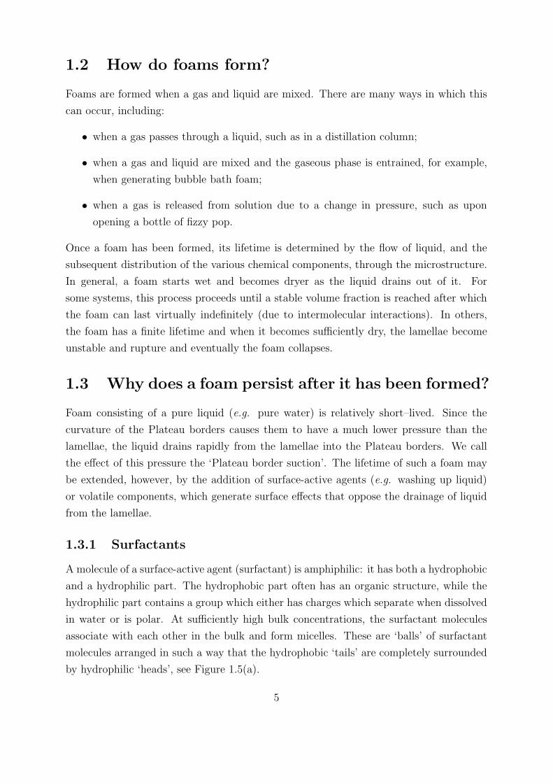
1.3.1 Surfactants
A molecule of a surface-active agent (surfactant) is amphiphilic: it has both a hydrophobic
and a hydrophilic part. The hydrophobic part often has an organic structure, while the
hydrophilic part contains a group which either has charges which separate when dissolved
in water or is polar. At sufficiently high bulk concentrations, the surfactant molecules
associate with each other in the bulk and form micelles. These are ‘balls’ of surfactant
molecules arranged in such a way that the hydrophobic ‘tails’ are completely surrounded
by hydrophilic ‘heads’, see Figure 1.5(a).
5

Surfactant molecules prefer to be present at an interface, rather than remaining in the
bulk. They arrange themselves so that the tail groups are in contact with the air, while
keeping the head groups within the liquid, see Figure 1.5(b). Adsorption of surfactant
(a)
AIR
FLUID
(b)
Figure 1.5: Surfactant molecules (a) forming a micelle and (b) at a free surface.
in this manner reduces the surface tension of the interface. We must thus consider two
species of surfactant molecules, namely those in the bulk liquid and those residing in the
surface.
Once the bulk concentration reaches the ‘critical micelle concentration’ (CMC), that is,
the concentration at which micelles first form, the surface tension does not change with
concentration. The surfactant molecules form more micelles rather than adsorbing at the
interface. Nonuniform adsorption due, for example, to an expanding surface, can therefore
result in a surface tension gradient.
1.3.2 How does a surface tension gradient affect a liquid flow?
A gradient in surface tension results in a surface shear stress acting on the liquid at the
surface. Viscosity transmits this shear into the liquid and hence the liquid is accelerated
or retarded, depending on the direction of the gradient relative to the bulk liquid flow.
This effect will tend to stabilise foam if the surface shear opposes the Plateau border
suction and conversely, the foam will be destabilised if the surface shear enhances the
Plateau border suction.
6

1.3.3 Volatile Components
A foam may also be stabilised if it contains a second, volatile, liquid component which
has a different surface tension from that of the primary liquid (e.g. in a heptane/toluene
mixture). Higher evaporation in one part of the system compared to another can lead
to depletion of the volatile component and hence a surface tension difference between
the two locations. If such a gradient of surface tension exists between the lamella and
Plateau border in a foam, the film may either be stabilised or destabilised, depending
on whether the volatile component has a higher or lower surface tension than the inert
component. In the Chemical Engineering literature, if the volatile component has the
lower surface tension, then the system is known as Marangoni Positive while if it has
the higher tension, then the system is known as Marangoni Negative (see Zuiderweg
and Harmens [82]). Marangoni positive systems readily foam, while Marangoni negative
systems do not foam at all. The former typically occur within distillation columns, where
their persistence is highly undesirable.
1.4 What happens to lamellae when they become
thin?
If a lamella is allowed to drain in a controlled environment, it may become so thin that
molecular forces arising from the interaction of the two free surfaces come into play. If
these forces are repulsive, this culminates in the formation of a stable “black” film of
thickness between 10 and 100 Angstroms.1 A very thin lamella may also be stabilised by
the formation of a solid surface layer, for example, in an ageing washing-up liquid foam.
Stabilisation of lamellae by these mechanisms will not be considered in this thesis. Our
concern is with foam that is fundamentally unstable, but whose lifetime may be extended
considerably by the mechanisms presented in §1.3.1 and §1.3.3.
1.5 How does a lamella rupture?
It is well known that a purely viscous film cannot break in finite time under the action
of a finite force. In practice, films spontaneously rupture when they become sufficently
thin. This may be due to random external fluctuations or to physical effects other than
viscosity and surface tension. Indeed, numerous authors have incorporated attractive
long-range intermolecular forces into thin-film models and thus predicted rupture at a
1One Angstrom is equal to 10−10m.
7

critical thickness. We do not concern ourselves here with the mechanics of the rupture:
we simply take this critical thickness to be a known material property.
1.6 How are foams destroyed in industrial situations
where they are not wanted?
There are two methods that are often used in industrial situations to break down foams.
1. Chemical breakdown: Chemicals that disperse foams are known as antifoams, and
are often oils or highly surface active materials. The choice of suitable antifoam
for a given foaming system is empirical, and an antifoam which works well for one
system may not work for another, similar system.2
2. Mechanical breakdown: Various mechanical methods can also be employed to break-
down foams. These range from the use of beaters (large stirring paddles within
the piece of industrial equipment) to using ultrasound, where the frequency is de-
termined to maximise foam destruction. Other methods include the use of heat
transfer.
Obviously, the method used depends crucially on the constitutive parts in the foam.
Attempting to break down a petrochemical foam using heat could be disastrous, for
example. Also these methods are all potentially costly, and it would be preferable to
avoid producing large quantities of foam in the first place.
1.7 Background material
There is a vast amount of literature on foams, both experimental and theoretical. We
present details of the work which is most relevant to this thesis in the appropriate chapters
that follow. General reviews of foam and its behaviour have been presented by Bikerman
[11], Kraynik [46] and Aubert, Kraynik and Rand [3]. Bikerman’s book focusses on
experimental observations and ad-hoc models for foams. Kraynik’s review includes more
theoretical aspects, while Aubert et al. provides an ‘easy-to-read’ account of foaming
phenomena.
Here, for completeness, we present an overview of some historically important and inter-
esting areas of foam research that we will not have space to touch on in the rest of this
thesis.2“When a plant has a foaming problem, the antifoam salesman is called, who turns up with a briefcase
full of chemicals. These chemicals are, in turn, introduced to samples of the foam in question. If thefoam is substantially reduced by one chemical, then it is introduced to the foaming solution.”-Darton [18].
8

More exotic foams
There are a variety of non-aqueous and non-volatile systems which foam. For example,
foams form on the top of molten baths of metal (such foams are known as Slag Foams).
It is not clear whether such foams are stabilised by the presence of surface-active impu-
rities or by small differences in temperature between the lamellae and Plateau borders.
Experimental work studying such foams is being undertaken by Nexhip [61].
Geometric work
The characteristic shape of foam bubbles depends on the coarseness of the foam. As noted
earlier, in a wet foam, bubbles are nearly spherical, while in a dry foam, the bubbles are
more polyhedral. Numerous authors have attempted to determine bubble shapes, all
trying to generate ideal cells: ones that tesselate space and minimise surface area.
Two-dimensional foams
As previously mentioned, Plateau [66] studied the joining of three lamellae (experimen-
tally), and concluded that they always meet at 120o. Weaire and Kermode [78, 79] describe
von Neumann’s bubble law which arises from a model to describe the change in area of
a two-dimensional bubble acting under only gas diffusion between bubbles and capillary
forces. The model predicts that bubbles with fewer than six sides shrink in area, whereas
bubbles with more sides grow.
Three-dimensional foams
When four lamellae meet, in three-dimensional space, they always join at an angle of
cos−1(1/3) (see Kraynik [46]). Planar films cannot satisfy this constraint, and so lamellae
must be curved. At the end of the last century, Lord Kelvin [74] created a tetrakaidec-
ahedron; a structure with six planar quadrilateral faces and eight non-planar faces, all
with curved edges, see Figure 1.6. He showed that it both tesselates space and minimises
surface area for a given volume. More recently, Weaire and Phelan [80] found that such
cells were present within a real foam. They also noted, from Matzke [57], that in practice
the commonest films in a foam are pentagonal. They constructed a collection of eight
polygonal bubbles which contains many pentagonal faces, fills space, and also has frac-
tionally less surface than a Kelvin cell. Kraynik and Reinelt [50, 47, 48, 49, 68] carried
out extensive work on the deformation of various theoretical foams. They used a surface
evolver, which computed the minimal surface at each stage of deformation, to find the
shape of a spatially periodic foam when shearing forces are applied.
9

Figure 1.6: The Kelvin Cell (courtesy of Andy Kraynik).
Figure 1.7: A random foam structure (courtesy of Andy Kraynik).
10

They used this to obtain shear moduli for the foams under consideration, which could
then be used to describe macroscopic properties of the foam. Of course, real foams are
often a random collection of bubbles, of various shapes and sizes, as shown schematically
in Figure 1.7.
Foam flow
The mechanism for foam flow is the slip of each bubble over its neighbours to a correspond-
ing position further along, see Figure 1.8. A critical yield stress is required to make this
Figure 1.8: Schematic of a layer of bubbles moving over the top of another layer.
step. Thereafter, the effective viscosity decreases with shear rate. As noted in Kraynik
[46], foams are macroscopically “multi-phase fluids which are compressible, nonlinear and
viscoelastic” and, typically, foam is consituted as a shear-thinning viscoplastic material.
A foam also exhibits slip at rigid boundaries. This can easily be seen as a macroscopic
description of flow of bubbles over a wetted surface. These properties should be derivable
from the microscopic flows that occur between the lamellae and Plateau borders.
There is a vast amount of work concerning foam flows in oil recovery processes. Here, the
size of the channel in which the foam flows may be only a few bubble diameters across.
Kornev et al. [22, 44], and Shugai [70] have discussed the flow of a foam within a porous
medium. The former performed experiments on bubble trains through a cavity as shown
in Figure 1.9. When the characteristic size of the bubbles was the same size as the inlet,
the bubbles moved through the cavity without disturbing those bubbles around the edge
of the chamber. When the characteristic size of the bubbles was much smaller than the
inlet, the motion of the bubbles in the cavity appeared totally random. A mathematical
study of flow of a bubble train through a porous medium was carried out in Kornev and
Kurdyumov [45].
11

Pressure gradient
Stationary bubbles
Direction of motion
Figure 1.9: Schematic of experiment to study a bubble train moving through a cavity.
1.8 Thesis plan
In Chapter 2, we present the basic models that underpin all the work that we carry out
in this thesis. We state the model for an incompressible Newtonian liquid, and we give
details of the boundary conditions at both rigid and free surfaces. We then state the
model for a soluble surfactant and formulate the boundary conditions for a surfactant
adsorbed at a free surface. Finally, we state the model for a volatile component in a
volatile-inert mixture, and discuss the boundary conditions that arise when we allow for
mass transfer across an interface.
In Chapter 3, we present details of an experiment to study how a surfactant affects a
dynamic interface in an easily accessible geometry, that of the overflowing cylinder. We
model both the liquid and the surfactant, and the interaction between the two. We
include the effects of gravity, capillarity, surface tension gradients, inertia and viscosity,
convection and diffusion of the surfactant, and diffusion-controlled adsorption onto the
surface. We have a high Reynolds number and high Peclet number flow and both diffusive
and viscous boundary layers exist at the free surface. A crucial observation is that the
diffusive boundary layer is typically much thinner than the hydrodynamic boundary layer.
We solve the outer problems for the liquid and the surfactant, and then solve the inner
problems close to the free surface, and in the vicinity of the stagnation point.
In Chapter 4, we develop the theory for thin films evolving under the action of Marangoni,
capillary and viscous forces. We derive the distinguished limits of the model, defined as
those regimes in which as many forces as possible balance. We also present other limits
in which two forces balance or one force dominates. We further describe the distribution
of the Marangoni inducing term, whether it is a surfactant or a volatile component.
In Chapter 5, we apply the thin film models derived in Chapter 4 to the problem of liquid
12

drainage from a lamella into a Plateau border. This involves decomposing the liquid
domain into a time-dependent lamella, a capillary-static Plateau border and a quasi-
steady transition region between the two. We first illustrate our procedure by considering
the evolution of a pure liquid film, for which an explicit solution to the problem has been
found. We solve the transition region problem to give the flux of liquid flowing from the
lamella into the transition region as a function of lamella thickness, and then, assuming
that the lamella is spatially independent, we are able to find the lamella thickness as
a function of time. We then turn our attention to a lamella stabilised by a well-mixed
surfactant, and we follow the same decomposition of the liquid domain as for the pure
liquid case. Our numerical solutions produce some interesting behaviour, which we explain
by an asymptotic analysis of the governing equations. We repeat the procedure using
parameters for the soluble surfactant CTAB, and for an insoluble pulmonary surfactant.
We present, but do not solve, the model for a lamella stabilised by a volatile component.
Finally, we show that we may make progress and obtain an explicit solution to the problem
if we assume that the system exhibits a constant surface viscosity rather than a Marangoni
stress.
In Chapter 6, we present an ad-hoc model for the flow in a single Plateau border. We use
this building block in a macroscopic model for a foam. We also discuss foam destruction
by a self-generated antifoam and by using hot wires.
In Chapter 7, we round off by presenting the important results from the previous chapters,
and by discussing extensions to our work. We finish by discussing experiments that we
feel would aid the advancement of the theory.
1.9 Statement of Originality
In Chapter 3, §3.4 onwards is original work. In Chapter 4, the identification of the velocity
scalings is original work, as are the models including Marangoni terms. The surfactant and
volatile models are original, except for the models where ε2Pe ∼ O(1) and the insoluble
surfactant model. The modelling has been presented in Breward, Darton, Howell and
Ockendon [14]. The work in Chapter 5 is all original, but the work in §5.2 is very similar
to that presented in Howell [38]. With the exception of the presentation of the so-called
Foam Drainage Equation, the work in Chapter 6 is all original.
13

Chapter 2
Modelling of liquids, surfactants andvolatile systems
In this chapter, we discuss the modelling of liquids, surfactants and volatile systems.
Our aim is to present the fundamental models for surfactant solutions and mixtures of
volatile and inert liquids flowing beneath a free surface. As noted in the introduction, the
surface tension of such solutions is not necessarily constant, and we describe the interplay
between the surface tension and the concentration field in each case. In general, the bulk
properties (such as density and viscosity) of a surfactant solution also vary with the bulk
concentration; see Pandit and Davidson [64]. Here we only consider the case where such
effects are negligible, and so we can treat the mixture as an incompressible Newtonian
liquid.
In the section that follows, we present an uncontroversial model and boundary conditions
to describe the velocity and pressure within the liquid. However, when we come to
modelling the surfactant, while the field equation (the convection-diffusion equation) is
well-known, the boundary conditions and the relationship between surface tension and
surfactant concentration are less obvious. We present a chemical justification for these
conditions, which, while not rigorous, gives some insight into the processes taking place.
Our faith in the conditions that we arrive at is born out by their ability to fit experimental
data (see Manning-Benson [52]). The model for a volatile component and the associated
boundary conditions are reasonably well established in the paint-drying literature (see
below).
For simplicity, we restrict ourselves to a two-dimensional geometry in this chapter. The
equations generalise to three dimensions in fairly obvious ways, and indeed, in Chapter 3
we employ the axially-symmetric version.
14

2.1 Liquid modelling
2.1.1 Field Equations
We employ the incompressible Navier-Stokes equations (see, for example, Ockendon and
Ockendon [62]) to describe the flow of our liquids. Thus u = (u(x, y, t), v(x, y, t)), the
velocity, and p, the pressure in the liquid, satisfy
∇.u = 0, (2.1)
ρ(ut + (u.∇)u) = −∇p+ µ∇2u− ρgj, (2.2)
where ρ is the density, µ is the constant viscosity and g is the acceleration due to grav-
ity (which we assume acts in the −j direction). The first of these equations represents
conservation of mass while the second represents conservation of momentum.
2.1.2 Boundary conditions
At any rigid boundaries, we impose the usual no-slip condition that the liquid in contact
with the boundary must move with the same velocity as the boundary. At a free surface
y = H(x, t), however, the boundary conditions are more complicated than the no-slip
condition, and involve force balances and kinematics. We utilise the unit tangent and
unit normal to the surface, defined by
t =±1
(1 +H2x)
12
(1Hx
), n =
±1
(1 +H2x)
12
(−Hx
1
), (2.3)
where we choose the sign of t and n so that the normal points outward from the liquid.
We denote the liquid stress tensor by τ , so for a Newtonian liquid we have
τ =
(−p+ 2µux µ (uy + vx)µ (uy + vx) −p+ 2µvy
). (2.4)
If σ is the surface tension of the liquid-gas interface, then balancing forces on a small
element of the surface, we obtain the relationships
±σκ = n.τ.n, (2.5)
∂σ
∂s= t.τ.n, (2.6)
where the (two-dimensional) curvature, κ, is given by
κ =Hxx
(1 +H2x)
32
, (2.7)
15

and s is arc length. Here, the liquid is on the right of the interface, when viewed along
the direction of s increasing, and we choose the sign in (2.5) to be consistent with the
definition of the normal in (2.3). We break with our usual convention of writing derivatives
as subscripts when we consider ∂∂s
and ∂∂n
. This is because s is a useful subscript to
denote surface quantities, and we wish to avoid confusion. Also, we use the quantity s to
denote volatile component later. On substituting for the stress tensor in these boundary
conditions, we find
±σκ = −p+ 2µvy − (uy + vx)Hx + uxH
2x
1 +H2x
, (2.8)
∂σ
∂s= µ
(uy + vx)(1−H2x)− 2(ux − vy)Hx
1 +H2x
. (2.9)
We shall refer to these two boundary conditions as the ‘normal force balance’ and the
‘tangential force balance’. The gradient of surface tension in the tangential force balance
is commonly known as a Marangoni stress.
We also require a third condition to locate the free surface. Assuming that there is no
evaporation, we employ the kinematic condition, which may be written as
v = Ht + uHx. (2.10)
We show how the kinematic condition can be modified to take account of evaporation in
§2.3 to follow.
2.2 Surfactants
We have previously mentioned that a surfactant has an affinity for a surface. Here, we
show how to model the transport of surfactant both in the bulk and on the surface. There
are two ways of describing the concentration. We choose to follow the surface chemistry
approach and to think of surfactant concentration as the number of moles of surfactant
in a unit volume (bulk surfactant) or area (surface surfactant). The other approach is to
use the volume fraction of surfactant molecules present in the solution.
As described in the previous chapter, some surfactants contain charged head groups which
dissociate when dissolved in water. Adsorption of surfactant at the free surface results in
the formation of an “electrical double layer”. Such a layer can hinder further transport
of surfactant to the surface. For simplicity, in this thesis we shall henceforth neglect such
effects.
16

We assume that the bulk surfactant is transported by convection and diffusion, and that
the concentration is below the critical micelle concentration, so that the dimensional
model for the bulk surfactant concentration, C(x, y, t) reads
Ct + (u.∇)C = ∇. (D(C)∇C) , (2.11)
where D(C) is the diffusivity of the surfactant which can, in general, vary with the
concentration of surfactant. We assume in this thesis, however, that the diffusivity is a
constant.
We assume that the concentration of surface surfactant Γ(x, t) (also known as the sur-
face excess) is also transported by convection and diffusion, but now we also allow for
an interchange of molecules with the bulk. We assume that such an interchange is con-
trolled by diffusion (although the process may also be controlled by activation energies
see Manning-Benson [52] or Chang [15] for a review), and so the flux from the bulk onto
the surface is
j = −D∂C∂n
. (2.12)
The equation for conservation of surfactant in the surface then reads
Γt +∂(usΓ)
∂s−Ds
∂2Γ
∂s2= j, (2.13)
where us is the surface velocity
us = u.t|y=H(x,t), (2.14)
and Ds is the surface diffusivity. In practice, surface diffusion is often negligible, and we
will neglect it henceforth, although we briefly examine its effects in the case of an insoluble
surfactant in §4.5.6 and §5.5. We call (2.13) the “replenishment condition”. The model
is closed by the constitutive relation for the flux j, which is in general of the form
j = j(C,Γ). (2.15)
The most common such model in the chemistry literature (see Chang [15]) sets the rate of
adsorption of surfactant at the surface to be proportional to the sub-surface concentration,
C(x,H, t), and to the amount of space available at the surface. The rate of desorption is
set proportional to the amount of surfactant on the surface, Γ. Hence we have the relation
j = k1 (C(Γ∞ − Γ)− k2Γ) , (2.16)
where Γ∞ is the “surface saturation concentration”, that is, the largest concentration
of surfactant that can be present at the surface, and k1 and k2 are material parameters.
17

Equation (2.13) along with the flux given by (2.16) is known as the Langmuir-Hinshelwood
equation (Chang [15]).
The three boundary conditions (2.12), (2.13) and (2.16) are sufficient to close the model
for C and Γ. They are often simplified further. Often, in practical situations we can
assume that the adsorption process described by (2.16) takes place very rapidly, and thus
k1 is, in some sense, large and (2.16) leads to a thermodynamic relation between Γ and
C known as the Langmuir isotherm (see Adamson [1]),
Γ =Γ∞C
k2 + C, (2.17)
which is then coupled with (2.12) and (2.13).
Another simplification occurs if the surfactant is insoluble (as is often the case for pul-
monary surfactant) in which case we can set j → 0 in (2.13) and ignore the problem for
C completely (see Gaver and Grotberg [29], for example).
2.2.1 Effect of surfactant on the surface tension
At a free surface, a surfactant is able to expel its hydrophobic tail from the solution and
this reduces the surface energy of the system. For our purposes, it is necessary to impose
the resulting constitutive relation between the surface tension and the surface concen-
tration. These relations are typically obtained experimentally, but to help explain the
origin of these effects, we present a “chemists’ model”. Our starting block is the modified
Gibbs equation which relates changes in surface tension to the surface concentration and
to changes in bulk concentration (Denbigh [24], Levich [51]),
δσ = −RTΓδC
C, (2.18)
where R is the universal gas constant and T is the temperature.1 Now, assuming thermo-
dynamic equilibrium, we use the Langmuir isotherm (2.17) to relate C to Γ, we let the
infinitesimals tend to zero, and integrate the equation to read
σ∗ − σ = −RT log
(1− Γ
Γ∞
), (2.19)
where σ∗ is the surface tension of pure water. Equation (2.19) is known as the Frumkin
equation (see Chang [15]). The term σ∗ − σ is sometimes called the “surface pressure”.
1Chemists use the concepts of (a) chemical potential and (b) an ideal-dilute solution to formulate thisrelationship. The RT factor in (2.18) arises because, at the surface, the surfactant is assumed to be inequilibrium with its vapour phase.
18
If the concentration of surfactant is above the critical micelle concentration (see §1.3.1),
we must include diffusion of micelles and interplay between the bulk and micellar concen-
trations. Such modelling is beyond the remit of this thesis.
2.3 Volatile and Inert systems
In general a foaming mixture may be formed by mixing any number of chemicals with
differing surface tensions and evaporation rates. In this thesis, we confine our attention to
the simplest case in which we have one volatile and one inert component. We model the
volatile component of an inert-volatile mixture by assuming that it forms a concentration
field within the liquid as a whole. Here, we define the concentration s(x, y, t) to be the mole
fraction of the volatile component, that is, the number of moles of the volatile component
compared to the total number of moles (of both the volatile and inert component) present.
We use this definition of concentration to be consistent with the experimentalists. We
propose that the mass transfer is controlled by convection and diffusion, and the model
reads
∇. (D(s)∇s) = st + (u.∇)s. (2.20)
Again, the diffusion coefficient may vary with the concentration of volatile component,
but in our modelling we will assume that it is constant.
2.3.1 Volatile component at the free surface
We must model two effects at the free surface: the first is evaporation of the volatile, and
the second is the dependence of the surface tension on the concentration s. We assume
that there is negligible adsorption of the volatile at the free surfaces, i.e., Γ ∼ 0, and we
only have to consider the bulk concentration. We consider the liquid evaporating at a
rate e(s) at a surface H(x, t), which moves with velocity Vn. At the surface we conserve
both volatile and inert components:
−Dsn + s (u.n− Vn) = e, (2.21)
Dsn + (1− s) (u.n− Vn) = 0. (2.22)
We eliminate the terms multiplying the velocities and we obtain
−Dsn = (1− s)e, (2.23)
which we may re-write as
−D(sy −Hxsx) = (1− s)e√
1 +H2x. (2.24)
19

If we eliminate the diffusion terms then we find
u.n− Vn = e. (2.25)
Noting that Vn = Ht/√
1 +H2x, and that u.n = (v − uHx)/
√1 +H2
x, we can we-write
(2.25) as
v = Ht + uHx + e√
1 +H2x, (2.26)
which is the kinematic condition re-written to include evaporation.
We denote the surface tension of the inert component by σI and that of the volatile
component by σV . We require our mixture to have these surface tensions when s is zero
or one respectively. However, the precise relationship that the surface tension follows
depends on the two components and how they interact (see Atkins [2] for a discussion of
how the partial pressures of binary mixtures behave). We assume that there is a linear
variation between the two values, and so we have
σ = σI +(σV − σI
)s. (2.27)
2.3.2 Model for evaporation
We must also pose a constitutive relation for how the evaporation rate e varies with the
concentration of volatile component s. Often, in applied mathematics literature, the rate
is taken to be equal to a constant, e.g., Howison et al. [39]. However, this does not
adequately take account of the fact that there is a finite amount of the volatile and that
the evaporation rate must be zero if the chemical potential in the liquid is the same as
in the vapour phase. We call s∗ the relevant concentration which makes the chemical
potentials equal. We introduce a mass transfer coefficient, E0, which is the velocity
associated with the movement of the free surface in the case when there is only volatile
present and the movement is due to evaporation alone. The simplest model that describes
this phenomenon is e = E0(s− s∗), but we assume that the gaseous mole fraction is small
and so work with
e = E0s. (2.28)
2.4 Summary
We have presented the models that underpin the rest of this thesis, with a chemical
justification of several of the conditions. We proceed to the next chapter where we hope
to check that, using the surfactant conditions presented here, we can describe the flow
20

of a surfactant solution in an experiment to measure the properties of an expanding free
surface.
We have closed our models by introducing extra chemistry relating to the surfactant or
volatile component. Another approach that is employed by some authors is to suppose
that the effect of a surfactant is to effectively stiffen the surface. Thus they pose a
relationship between the surface tension and the surface velocity. The simplest such model
sets the surface velocity equal to zero (for example, Schwartz and Princen [69]), while more
elaborate, but still phenomenological models propose the use of a “surface viscosity”, i.e.,
the surface layer is treated as a viscous liquid with a different viscosity from the bulk
liquid (for example Dey et al. [27]). In such a case, the surface tension is set to be equal
to the surface viscosity multiplied by the rate of strain of the surface. Another similar
approach is to model the surface as a elastic membrane, with a corresponding “surface
elasticity”. We believe that these effects can be thought of in terms of the surface tension
gradient and hence do not need to be introduced if the chemistry and thermodynamics
of §2.2 is justifiable macroscopically. At appropriate points through this thesis, we shall
discuss our model’s relationship to those in which surface viscosity is used in place of the
Marangoni term.
21

Chapter 3
Modelling expanding free surfaces
3.1 Introduction
In Chapter 5 we will explore the way in which surfactant acts to stabilise a foam. A
crucial property of surfactant in this respect is the way in which it resists expansion
of the gas/liquid interface. However, making experimental measurements on such free
surfaces is a difficult task since the lamellae are not only very thin, but are often also
inaccessible. However, some ingenious experiments have been devised whereby expanding
free surfaces can be studied and the effect of surfactant on them determined, the idea
being to verify the boundary conditions proposed in Chapter 2. In these systems, the
presence of surfactants affects the properties of the flow close to the free surfaces.
We turn our attention to two experiments that have been carried out within the Physical
and Theoretical Chemistry Laboratory at Oxford University. The first experiment, using
an overflowing cylinder, will be described in detail below. We shall also briefly describe
the second experiment, which uses a jet of liquid, in Chapter 7. Both these experiments
exhibit surface lifetimes comparable to those in foams.
3.2 The overflowing cylinder
The overflowing cylinder (OFC) is a device to measure the properties of an expanding free
surface. It consists of a glass or metal cylinder (longer than it is wide) mounted with its
axis vertical on a platform designed to minimise externally induced vibrations. Liquid is
forced by a pump up the cylinder at a low flow rate so that, on reaching the top, it flows
outward towards the rim of the cylinder and then smoothly overflows down the outside.
It is then collected and re-circulated (see Figure 3.1). Flow straighteners near the base
of the cylinder aim to ensure that uniform plug flow is achieved at a distance from the
free surface. Using various techniques (including Laser Doppler Anemometry, Neutron
22

PUMP
FLOWMETER
RESISTANCEPLATE
FLOWSTRAIGHTENER
Figure 3.1: The overflowing cylinder.
Scattering and Ellipsometry), the shape of the top surface, the surface tension, the surface
velocity and the surface concentration of any added surfactant can be determined at
various points on the surface. These techniques are non-invasive, i.e., they do not disturb
the flow (unlike conventional techniques such as the Wilhelmy plate, see Manning-Benson
[52]). The experimental techniques are reviewed in Manning-Benson et al. [52, 54, 55, 56].
We show a close-up of the overflowing cylinder in Figure 3.2. The arrows indicate the
direction of the flow at the bottom of the cylinder, close to the free surface, and in the
wetting film on the outside wall. The free surface at the top of the OFC is continually
expanding, and, when a surfactant is present, surface tension gradients at this surface
may be generated. By taking measurements of these gradients in a controlled system, we
hope to learn about surface shear forces and adsorption of surfactant.
23

r
z
plug flow
expanding free surface
Wetting film
Figure 3.2: Close-up of the overflowing cylinder.
3.3 Previous work
Several authors have published details of experimental and theoretical work on the over-
flowing cylinder. Bergink-Martens et al. [7, 8, 9] formulated a boundary-layer model for
the flow close to the surface, assuming that the flow at depth was given and that the
surface tension gradient was known. Darton et al. [31] also attempted a boundary-layer
approach in the modelling of their experiments. Gillow [30] formulated inviscid models in
both two-dimensional and axially-symmetric geometries and solved these using analytical
and numerical methods. Manning-Benson has described her recent experiments in the
papers mentioned above.
Jensen [41] has formulated a model in the related area of insoluble surfactants on deep
water and Harper [33, 35] has formulated a model in the related area of a bubble rising
in a dilute solution of soluble surfactant.
Our new contribution is to couple the hydrodynamic problem (incorporating an inviscid
outer flow and a viscous boundary layer at the free surface) with the surfactant problem
via the momentum and mass balances and the continuity of shear and replenishment
boundary conditions.
24

3.3.1 Experimental observations
Manning-Benson has carried out a variety of experiments using hexadecyltrimethylam-
monium bromide (CTAB), which is a cationic surfactant, and is shown in Figure 3.3. We
CH3
CH3
CH3
N Br−+
C
Figure 3.3: Display formula for CTAB.
present some of her experimental results and observations below. The measurements were
restricted to a region within 2–3 cm of centre of the cylinder (whose radius was 4 cm).
We comment that the measurements were made in a line across the free surface, and r
here denotes distance from the centre, measured along this line (i.e. r can be negative).
1. Speed
Figure 3.4 shows surface speed measurements versus the distance r from the axis,
for a number of bulk surfactant concentrations and Figure 3.5 shows the surface
speed for pure water.
Figure 3.4: Surface speed measurements (Vr measured in mm s−1) against distance (rmeasured in mm), for a number of bulk concentrations.
25

Figure 3.5: Surface speed measurements (Vr measured in mm s−1) against distance (rmeasured in mm), for pure water.
We note that:
• with surfactants in the system, the speed of the liquid at the free surface is
markedly faster than the surface speed associated with pure water;
• the surface velocity appears to vary approximately linearly with distance.
We attribute the apparant ‘kink’ in the pure water speed profile in Figure 3.5 to
experimental error. Figure 3.6 shows the change of horizontal speed with distance
away from the surface, at different stations across the cylinder. The concentration
of CTAB is 0.58 mol m−3 in this case. We note that the liquid is accelerated in a
small region close to the top surface of the liquid.
2. Bulk concentration versus surface concentration
Figure 3.7 shows the variation of surface concentration with bulk concentration,
measured under static conditions. The data have been fitted with a Langmuir
isotherm. As mentioned in Chapter 2, there is a timescale associated with the
adsorption onto the surface. We hope that this timescale is much shorter than any
other timescale in the problem, so that the Langmuir isotherm may be employed
under our dynamic conditions.
26

Figure 3.6: Horizontal speed (Vr in mm s−1), for a number of depths (h in mm), atr = 6mm (circles), r = 12mm (triangles) and r = 20mm (upside down triangles).
Figure 3.7: The Langmuir isotherm.
27

Figure 3.8: Variation of surface tension (σ in mN m−1) with distance across the cylinder(r in mm), for various bulk concentrations: (a) 0.1, (b) 0.17, (c) 0.25, (d) 0.31, (e) 0.35,(f) 0.46, (g) 0.51, (h) 0.58, (i) 0.68, (j) 0.81 mol m−3.
3. Surface Tension
Figure 3.8 shows the surface tension, measured under dynamic conditions, for vari-
ous bulk concentrations (from Manning-Benson [52]). We note that:
• the surface tension varies only slightly across the cylinder and does so roughly
quadratically;
• the surface tension is lowest at the centre of the surface.
We show the variation of surface tension with bulk concentration, measured under
static conditions, in Figure 3.9. Note that, in experiments, it is the bulk concen-
tration of the surfactant solution that is initially known, rather than the surface
concentration. By comparing the data in Figure 3.9 with the surface tension at the
centre of the cylinder in Figure 3.8, we see that the surface tension at the centre
is higher when the measurement is made under dynamic conditions than when the
measurement is made under static conditions.
4. Surface Concentration
Figure 3.10 shows the variation of surface concentration across the cylinder, for
various values of the bulk concentration. We note
28

Figure 3.9: Variation of surface tension (σ0 in mN m−1) with bulk concentration (C inmol m−3) measured under static conditions.
• the concentration appears to be almost constant, and the variation to this
constant appears quadratic;
• the concentration is largest in the centre of the surface;
Using the Langmuir isotherm to convert bulk concentration to surface concentration,
and then comparing this surface concentration to the central values in Figure 3.10,
we can infer that the surface concentration is lower under dynamic conditions than
under static conditions.
5. Other experimental observations
• Experiments were performed using cylinders with different radii (3, 4 and 5
cm). The velocity and concentration profiles were virtually unaffected by these
changes.
• Various flanges were inserted into the cylinder to change the curvature at the
rim. Such changes did not affect the measurements on the surface.
• It was found that, so long as the wetting film on the outside of the cylinder was
sufficiently long, it did not affect the behaviour on the expanding free surface.
Subsequently, all experiments were performed above this critical length.
29

Figure 3.10: Variation of surface concentration (Γ in mol m−2) with distance across thecylinder (r in mm), for various bulk concentrations: 0.1 mol m−3 (black triangles), 0.31mol m−3 (open circles), 0.58 mol m−3 (black diamonds), 0.81 mol m−3 (open triangles)and 1.73 mol m−3 (black squares).
30
• The flow rate was varied, and above a critical flow rate, the surface velocity
did not change as the flow rate was altered. The experiments were carried out
above this critical flow rate.
• In the case of pure water, the deviation of the free surface from horizontal was
more pronounced than in the surfactant cases, where the deviation was very
small.
3.3.2 Plan
We model both the liquid velocity and the distribution of surfactant, and show that
the model exhibits the qualitative experimental behaviour described above. We then
compare our results for surface tension, surface velocity and surface concentration with
those obtained experimentally.
3.4 Model formulation: velocity distribution
We consider the situation shown in Figure 3.2. We use the axially symmetric form of the
model presented in Chapter 2, and, since all the measurements at the surface are made
in a steady state, we assume that the velocities and the height of the free surface do not
vary with time. The steady axially symmetric Navier-Stokes equations are
ρ (uur + wuz) = −pr + µ
(1
r(rur)r −
u
r2+ uzz
), (3.1)
ρ (uwr + wwz) = −pz + µ
(1
r(rwr)r + wzz
), (3.2)
1
r(ru)r + wz = 0, (3.3)
where p is the reduced pressure (see Batchelor [6]), and the boundary conditions at free
surface z = H(r) read
σκ = −p+ ρgH + 2µwz − (uz + wr)Hr + urH
2r
1 +H2r
, (3.4)
σr = µ(uz + wr)(1−H2
r )− 2Hr(ur − wz)√1 +H2
r
, (3.5)
w = uHr, (3.6)
where u is the horizontal velocity, w is the vertical velocity, H is the free surface shape,
and r and z are as shown in Figure 3.2. At depth, we assume plug flow,
w → Ud, u→ 0, z → −∞. (3.7)
31

and at the cylinder walls we apply the no-slip condition
u = 0, at r = a, (3.8)
where a is the radius of the cylinder. Finally, we assume symmetry about the centre-line
of the cylinder:
u = wr = Hr = 0, at r = 0. (3.9)
We note that (3.7) and (3.8) are inconsistent. In place of (3.7) we should really pose
the condition that the flow straighteners give rise to plug flow at a finite depth in the
cylinder. However, the actual flow through the straighteners is unknown, and is likely to
be much more complicated than just plug flow. Hence, to stay clear of having to address
this flow problem, we assume that the flow straighteners are at “−∞”. Of course, if we
were concerned with flow close to the wall, we would have to deal properly with these
inconsistencies, but we do not bother since we are most interested in the flow at the free
surface, where all the available evidence suggests that the flow at depth is unimportant.
We proceed by nondimensionalising the field equations and boundary conditions (3.1)–
(3.9), settingu = Udu
′, v = Udv′,
r = ar′, z = az′,
p = ρU 2dp′, σ = γ0 + σ′∆γ,
(3.10)
where γ0 is the (unknown a priori) surface tension of the surfactant solution at the centre
of the cylinder, and ∆γ is the size of the surface tension change across the cylinder (which
we will later relate to the change in surface concentration). The field equations become
(dropping primes)
uur + wuz = −pr +1
Re
(1
r(rur)r −
u
r2+ uzz
), (3.11)
uwr + wwz = −pz +1
Re
(1
r(rwr)r + wzz
), (3.12)
1
r(ru)r + wz = 0, (3.13)
while the boundary conditions are
(1
CaRe+
Ma
Reσ
)κ = −p+
H
Fr2 +2
Re
wz − (uz + wr)Hr + urH2r
1 +H2r
, (3.14)
Maσr =(uz + wr)(1−H2
r )− 2Hr(ur − wz)√1 +H2
r
, (3.15)
32

w = uHr, (3.16)
on z = H, and
w → 1, u→ 0, z → −∞, (3.17)
u = 0, r = 1, (3.18)
u = 0, Hr = 0, r = 0. (3.19)
We have introduced four dimensionless groups describing various force balances: the
Marangoni number Ma, the Reynolds number Re, the capillary number Ca and the Froude
number Fr, given by
Ma =∆γ
µUdRe =
ρaUdµ
Ca =µUdγ0
Fr2 =U2d
ga. (3.20)
The behaviour of the system of equations depends crucially on the size of these groups,
and so we now consider typical physical parameter sizes.
3.4.1 Typical non-dimensional parameter sizes based on flow atdepth
We use the following values, based on the Manning-Benson experiments, in calculating
the sizes of the nondimensional groups:
ρ ∼ 1× 10³ kg m−3,
µ ∼ 1× 10⁻³ kg m−1 s−1,
γ0 ∼ 5× 10⁻² N m−1,
∆γ ∼ 2× 10⁻³ N m−1,
a = 3× 10⁻²–5× 10⁻² m,
Q = flux at depth = 1.6× 10⁻⁵ m3 s−1,
Ud = Q/(πa2) = 3.2× 10⁻³ m s−1 when a = 0.04 m,
(3.21)
whence,
Re ∼ 130, Ma ∼ 630, Ca ∼ 6.4× 10⁻⁵, Fr2 ∼ 2.5× 10⁻⁵. (3.22)
We use the size of these parameters to make qualitative statements about the flow.
• Since Re >> 1, the flow is inertia dominated away from the free and fixed surfaces.
• In (3.14), the capillary term 1/(CaRe) ∼ 102, the gravity term 1/Fr2 ∼ 4× 10⁴ and
the viscous term 1/Re ∼ 10−2. Hence the normal force balance is dominated by
33

gravitational forces, and since, from (3.14), Hx ∼ O(Fr2/(CaRe)) = O(3 × 10⁻³),
the free surface is forced to be flat to lowest order, as seen in the experiments.
Henceforth, we shall assume that the free surface is flat at z = 0, without loss
of generality, and we no longer need to work with the normal force balance. We
consider relaxing this assumption in §3.10.2.
• In (3.15), the Marangoni term Ma ∼ 630 and so we conclude that surface tension
gradients dominate the flow close to the free surface.
3.5 Model formulation: surfactant distribution
We now formulate the convection–diffusion problem for the surfactant. We work with the
axially-symmetric form of the equations and boundary conditions presented in Chapter
2, which read
D
(1
r(rCr)r + Czz
)= uCr + wCz, (3.23)
with boundary conditions at the free surface
Γ =Γ∞C
k2 + C, (3.24)
DCz = −1
r(ruΓ)r. (3.25)
At depth, we assume that the concentration of surfactant is constant,
C → Cb, z → −∞, (3.26)
where Cb is the known concentration of the surfactant solution added to the system. At
the edge of the cylinder there is zero flux:
Cr = 0, r = a, (3.27)
and we assume symmetry about the centre-line, so that
Cr = 0, Γr = 0, r = 0. (3.28)
We nondimensionalise the bulk concentration with its value at depth,
C = CbC′. (3.29)
However, more care is needed in choosing the most appropriate scaling for the surface
concentration. Experimental observations indicate that Γ varies by a fairly small amount
across the surface, but its value at the axis, Γ∗ say, is unknown a priori. We suppose
34

0.2 0.4 0.6 0.8 1 1.2 1.4
1·10-6
2·10-6
3·10-6
4·10-6
C
Γ
Γ∗
Υ∗
Figure 3.11: Langmuir isotherm showing Υ∗, Γ∗ and the variation of Γ and C at thesurface (in red).
that the sub-surface concentration corresponding to Γ∗ is Υ∗, see Figure 3.11. We nondi-
mensionalise Γ in such a way that the slope of the graph of Γ and C at Γ = Γ∗ is 1. We
therefore set
Γ =k2Γ∞Cb
(k2 + CbΥ)2Γ′, (3.30)
where Υ = Υ∗/Cb is the dimensionless value of the subsurface concentration at the centre
of the cylinder (which we emphasise is unknown a priori).
The field equation becomes (dropping primes)
1
r(rCr)r + Czz = Pe (uCr + wCz) , (3.31)
with boundary conditions at the free surface z = 0
Γ =(k2 + CbΥ)2C
k2(k2 + CbC)= λΥ2 + C − λ(C −Υ)2
1 + λC, (3.32)
SCz = −1
r(ruΓ)r, (3.33)
while
C → 1 as z → −∞. (3.34)
We introduce three further dimensionless groups: the Peclet number Pe, the replenishment
number S, and λ given by
Pe =Uda
DS =
D(1 + λΥ)2
UdΓ∞λ =
Cbk2
. (3.35)
35

We close the model by specifing the relationship between the surface tension and surface
concentration, which, after the chosen nondimensionalisation, reads
σ∗ − γ0
RTΓ∞− ∆γ
RTΓ∞σ = − log
(1− λΓ
(1 + λΥ)2
), (3.36)
3.5.1 Linearisation
Now we simplify the above problem further by linearising the Langmuir isotherm (3.32)
and the Frumkin equation (3.36). Our aim is to obtain more tractable boundary condi-
tions which still retain the important physical mechanisms of coupling between the bulk
concentration, surface concentration and surface tension.
We use the experimental observation in §3.3.1 that Γ does not vary much across the
cylinder to motivate our linearisation. We shall check a posteriori that this assumption
is correct in §3.9.3.
We linearise (3.32) about the sub-surface centre concentration Υ to obtain
Γ = λΥ2 + C, (3.37)
and from here onwards we work with (3.37) in place of the more complicated (3.32). We
note that this is equivalent to replacing the Langmuir isotherm with the straight line
segment shown in red in Figure 3.11. We substitute Γ into the replenishment condition,
which then reads
SCz = −1
r
(ru(λΥ2 + C
))r. (3.38)
Finally, we substitute Γ from (3.32) into (3.36),
σ∗ − γ0
RTΓ∞− ∆γ
RTΓ∞σ = − log
(1
1 + λC
). (3.39)
We linearise (3.39) about C = Υ, and we find
σ∗ − γ0
RTΓ∞− ∆γ
RTΓ∞σ = − log
(1
1 + λΥ
)+
λ
1 + λΥ(C −Υ), (3.40)
and so, setting
γ0 = σ∗ +RTΓ∞ log
(1
1 + λΥ
), (3.41)
and
∆γ =RTΓ∞λ
1 + λΥ, (3.42)
we obtain the simple relation between σ and C
σ = Υ− C. (3.43)
36

3.5.2 Nondimensional parameter sizes based on flow at depth
In addition to the values given in §3.4.1, we also use
D ∼ 5× 10⁻¹⁰ m2 s−1
k2 ∼ 0.127 mol m−3
Γ∞ ∼ 4.26× 10⁻⁶ mol m−2.
(3.44)
To calculate Pe, S and λ, we must choose a value of Cb and use the experimental results
to estimate Υ. For Cb = 0.58 mol m−3, we have Υ = 0.4. Hence we find
Pe ∼ 2.5× 10⁵, S ∼ 3.7× 10⁻², λ ∼ 4.6. (3.45)
These parameters indicate that convection dominates the problem away from the free
surface.
3.6 Outer (Inviscid) Problem
We first consider the “outer” region where the flow is inviscid to leading order. We expand
the dependent variables in terms of Re−1 and the leading-order outer liquid problem
becomes
u0u0r + w0u0z = −p0r, (3.46)
u0w0r + w0w0z = −p0z, (3.47)
1
r(ru0)r + w0z = 0. (3.48)
These are the Euler equations for an inviscid flow, which are a singular limit of the
Navier-Stokes equations in which the highest derivatives have been dropped. Thus, the
only boundary conditions that we can apply are the kinematic condition (the normal force
balance has already led to the conclusion that H = 0), the normal velocity condition at
the edge of the cylinder, the matching condition at depth and the symmetry condition
at the axis. The tangential components can only be applied when we consider viscous
boundary layers. The associated boundary conditions therefore read
w0 = 0 on z = 0, (3.49)
w0 ∼ 1 as z → −∞, (3.50)
u0 = 0 on r = 1, (3.51)
u0 = 0 on r = 0. (3.52)
We recast the problem in terms of a stream function ψ, so that u0 = 1rψz, w0 = −1
rψr.
Since the flow is clearly irrotational, we arrive at the following model for ψ
37

ψrr −ψrr
+ ψzz = 0, (3.53)
with
ψ = 0 on z = 0, (3.54)
ψ ∼ −1
2r2 as z → −∞, (3.55)
ψ = −1
2on r = 1, (3.56)
ψ = 0 on r = 0. (3.57)
3.6.1 Inviscid solution
To solve the system (3.53)-(3.57), it is useful to make the substitution χ = ψ + 12r2. The
problem becomes
χrr −χrr
+ χzz = 0, (3.58)
with
χ =1
2r2 on z = 0, (3.59)
χ = 0 on r = 0, (3.60)
χ = 0 on r = 1, (3.61)
χ→ 0 as z → −∞. (3.62)
We can find the solution, for example, by letting z = −z ′ and then peforming a sine
transform, i.e. setting
χ(r, k) =
∫ ∞
0
χ(r, z′) sin(kz′)dz′. (3.63)
The equation for χ is
χrr −χrr− k2χ = −k
2r2, (3.64)
and, after applying the boundary conditions we find the solution is
χ =r2
2k− rI1(kr)
2kI1(k), (3.65)
where I1 is the modified Bessel function of the first order. So, inverting,
χ =2
π
∫ ∞
0
sin(kz)
(r2
2k− rI1(kr)
2kI1(k)
)dk, (3.66)
which gives us
38

ψ =r
π
∫ ∞
0
I1(kr) sin(kz)
kI1(k)dk. (3.67)
Hence, the liquid velocities are given by
u0 =1
π
∫ ∞
0
I1(kr) cos(kz)
I1(k)dk, w0 = − 1
π
∫ ∞
0
I0(kr) sin(kz)
I1(k)dk. (3.68)
The velocity field given by (3.68) is shown in Figure 3.12. For subsequent matching, we
require the velocity at the top surface, say
uout(r) =1
π
∫ ∞
0
I1(kr)
I1(k)dk. (3.69)
Near to the origin this has the behaviour
uout(r) ∼r
2π
∫ ∞
0
k
I1(k)dk +
r3
16π
∫ ∞
0
k3
I1(k)dk +O
(r5), (3.70)
which, on evaluating, becomes
u0(r, 0) ∼ 0.89r + 0.67r3 + . . . . (3.71)
A comparison between the expansion and the exact solution, for r between 0 and 0.5 is
shown in Figure 3.13.
We may also examine the behaviour of the solution near to the rim. Firstly, we substitute
s = kr and then we let r = 1− εr′ and z = εz′. Then u becomes
u =1
π(1− εr′)
∫ ∞
0
I1(s)
I1
(s
1−εr′) cos
(εz′s
1− εr′)ds. (3.72)
To proceed we must split the range of integration since the integrand has different asymp-
totic behaviour when s ∼ O(1) and when s ∼ O(1/ε). We choose to split the range of
integration into (0, 1/√ε), (1/
√ε,∞), although any power of ε between zero and one will
do. We also utilise the asymptotic form for I1(s) when s is large:
I1(s) ∼ 1√2πs
es. (3.73)
After some grisly algebra, we find
u ∼ 1
π(1− εr′)
∫ 1/√ε
0
I1(s)
I1
(s
1−εr′) cos
(εz′s
1− εr′)ds+
e−√εr′
1−εr′(r′ cos
√εz′
1−εr′ − z′ sin√εz′
1−εr′)
πε√
1− εr′(r′2 + z′2),
(3.74)
39

0 0.2 0.4 0.6 0.8 1r
-1.5
-1.25
-1
-0.75
-0.5
-0.25
0
z
Figure 3.12: Plot showing the inviscid velocity field.
40

0.1 0.2 0.3 0.4 0.5r
0.1
0.2
0.3
0.4
0.5
u
Figure 3.13: Graph showing the solution, (3.69), for u (in black), compared with theexpansion (3.71), for u (in red).
and, expanding both the integral and the second term in powers of ε and then substituting
for the original variables, we find that
u(r, z) ∼ 1− rπ((1− r)2 + z2)
. (3.75)
We may also find the form of w in a similar way,
w ∼ − z
π((1− r)2 + z2). (3.76)
The rim may therefore be viewed as a sink, strength 2 (as might have been anticipated
from the boundary conditions).
We note that
• the solution satisfies uz = 0 on z = 0. Thus this condition satisfies the tangential
boundary condition on z = 0 exactly if the Marangoni number is zero (i.e. if there
is no surfactant present). However, when Ma 6= 0, (3.15) is not satisfied and so we
must introduce a viscous boundary layer near z = 0. We consider the boundary
layer problem in §3.8.1.
• the inviscid solution does not satisfy the boundary condition w0 = 0 on r = 1. In
order to satisfy this condition, we should reintroduce the viscous terms close to the
edge. However, since our main interest is in the free surface we hope we will not
need to analyse flow near r = 1 in detail.
41

3.7 Outer (surfactant) Problem
In (3.31) the Peclet number, which we recall is large, plays the same role as the Reynolds
number does in the hydrodynamic problem. As in the liquid case, the limit Pe → ∞ is
singular, since Pe multiplies the highest derivative in the system. Thus, again, we will not
be able to satisfy all of the boundary conditions at the free surface and at the edge of the
cylinder with this “outer” solution. We introduce a diffusive boundary layer near z = 0
in §3.8.2. Here, we expand (3.31) in powers of 1/Pe, and we find that to leading-order,
the surfactant concentration satisfies
u0C0r + w0C0z = 0, (3.77)
and so C0 is constant along the streamlines. So, since we have
C0 → 1 as z → −∞, (3.78)
we deduce that the concentration must be C0 = 1 everywhere in the outer region.
3.7.1 Solution to the problem in the limit Ma→ 0 and S →∞In §3.6.1 we noted that the leading-order outer solution actually satisfies the correct
boundary conditions on z = 0 when Ma = 0. Similarly, the solution C = 1 satisfies the
replenishment condition in the limit S →∞. Thus in the limit Ma→ 0 and S →∞, we
have u→ u0 and w → w0, as given by (3.68) and the solution to the surfactant problem
reads
C0 = 1, Γ0 = 1 + λ, σ = 0. (3.79)
We note that, for example, for Cb = 0.58 mol m−3, we have Γ = 5.57, which corresponds
to a dimensional value of 3.5 × 10⁻⁶ mol m−2. This is the value that we would have
expected for the surface concentration if it had been measured under static conditions.
However, if we read off the experimental value of Γ at the centre of the free surface from
Figure 3.10, we find that Γ ∼ 2.75× 10⁻⁶ mol m−2. Hence, we conclude that the value of
Γ given by (3.79) is higher than the experimentally observed value.
3.8 Boundary layers at the free surface
When we have nonzero Marangoni and inverse replenishment numbers, the solutions above
fail to satisfy the continuity of shear and the replenishment boundary conditions. We
therefore seek both hydrodynamic and diffusive boundary layers beneath the free surface.
Recall that in the outer solutions described above, the velocity is scaled with Ud and
42

lengths all scale with a. However, as indicated in §3.3.1 the behaviour of the surface ve-
locity and concentration is observed experimentally to be independent of both Ud and a.
This motivates us to allow the boundary layer problems to select not only the thicknesses
of the two boundary layers, but also the velocity scaling and the lengthscale of the prob-
lem. We scale the vertical hydrodynamic length and the vertical velocity by ε, and the
corresponding diffusive length by δ. We replace the radius, a by L, and the velocity Ud
by U in each of the dimensionless groups (namely Re, Ma, Pe and S). Setting ε2Re = 1,
δ2Pe = 1, εMa = 1 and S/δ = 1, we have four equations for the four unknowns L, U , ε
and δ, and we find that the relevant scalings are
U =
(DR2T 2C2
b
ρµ
) 14
(1 + λΥ)12 ,
L =
(R2T 2C2
bΓ8∞
D3ρµk82
) 14
(1 + λΥ)−72 ,
ε =
(Dµ3k4
2
ρR2T 2Γ4∞C
2b
) 14
(1 + λΥ)32 ,
δ =
(D3ρµk4
2
R2T 2C2bΓ4∞
) 14
(1 + λΥ)32 .
(3.80)
All the scalings contain the (unknown) sub-surface centre concentration, Υ, which will
be determined during the solution of the problem. We note before continuing that, using
Υ = 0.4, which is the nondimensionalised experimental value for Cb = 0.58 mol m−3,
U ∼ 0.3 m s−1, L ∼ 0.01 m, ε ∼ 0.018, δ ∼ 4× 10⁻⁴. (3.81)
There are several interesting ratios that we can make from the above scalings. The first
is the ratio of the two boundary layer thicknesses
δ
ε=
(ρD
µ
) 12
= Pr12 , (3.82)
where Pr, the Prandtl number, is a property only of the surfactant-liquid system under
consideration. For example, in an aqueous CTAB solution, Pr12 ∼ 0.022, and indeed we
can expect all systems of practical interest to have Pr << 1. We conclude that the diffusive
boundary layer (known hereafter as DBL) is always much thinner than the hydrodynamic
boundary layer (HBL). We will use this ratio when considering the coupling between the
hydrodynamic and diffusive problems.
The next ratio of interest is V = Ud/U , the ratio of the velocity at depth to the intrinsic
velocity scale. Using Υ = 0.4, we calculate V ∼ 1 × 10⁻². Hence our intrinsic velocity
43

scale is much larger than the the velocity at depth, as supported by the experimental
evidence.
The final interesting ratio is l = L/a, the ratio of the intrinsic lengthscale to the radius
of the cylinder. Again we use Υ = 0.4, and we find that l = 0.2625. Hence, our intrinsic
length scale is less than the radius of the cylinder and this suggests the presence of an
“inner region” close to the axis of the cylinder (where the experimental measurements are
taken).
3.8.1 The hydrodynamic boundary layer
Now we re-nondimensionalise the equations and boundary conditions using the above
scalings, i.e., scaling r = Lr, z = εLz, u = Uu and w = εUw. We only consider the
leading-order solution in ε and thus simply set ε = 0 in the resulting equations, which
then read
uur + wuz = −pr + uzz, (3.83)
pz = 0, (3.84)
1
r(ru)r + wz = 0. (3.85)
From (3.84), the pressure is only a function of r and, if we substitute for a stream function,
ψ so that the conservation of mass equation (3.85) is automatically satisfied (i.e. u = 1rψz,
w = −1rψr again), then we obtain
ψzzz =1
r
[ψzψzr − ψrψzz −
1
rψ2z
]+ p′(r). (3.86)
Now, matching with the flow at depth gives
ψ ∼ V rzuout(lr) as z → −∞, (3.87)
where uout is the outer velocity found earlier,
uout(t) =1
π
∫ ∞
0
I1(kt)
I1(k)dk. (3.88)
Thus,
p′(r) = −V 2lruout(lr)u′out(lr). (3.89)
In terms of the stream function, the boundary conditions at the free surface reduce to
ψ = 0 on z = 0, (3.90)1
rψzz = σr on z = 0. (3.91)
44

3.8.2 The diffusion boundary layer
In the diffusion boundary layer, height is scaled with δL, and so we set z = δLζ, and then
the leading-order surfactant problem reads
Cζζ = uCr +ε
δwCζ , (3.92)
with boundary conditions
−Cζ =1
r
(ru(λΥ2 + C
))r, (3.93)
at the free surface ζ = 0 and
C → 1, ζ → −∞. (3.94)
At first glance it may appear inconsistent to keep in the ε/δ term in (3.92), but we note
that w(r, z) = w(r, δζ/ε) = O(δ/ε) as δ → 0 so that this term is O(1) as δ → 0.
3.8.3 Coupling between the hydrodynamic and diffusive prob-lems
The coupling between the hydrodynamic and diffusive problems works both ways. Firstly,
the diffusive problem is driven by the velocity field (u, w). This coupling can be simpli-
fied by using the fact that the ratio of the boundary layer thicknesses is small, i.e., by
expanding (3.92) in the limit as δ/ε→ 0. The result of this is that the diffusion problem
only depends on the velocity field evaluated at the free surface:
Cζζ =1
r
[ψz(r, 0)Cr − ψrz(r, 0)ζCζ
], (3.95)
with
Cζ(r, 0) = −1
r
(ψz(r, 0)
(λΥ2 + C(r, 0)
))r
on ζ = 0, (3.96)
C → 1 as ζ → −∞. (3.97)
The concentration C is coupled back to the hydrodynamic problem through the surface
tension, given by (3.43). Thus, the streamfunction ψ satisfies
ψzzz =1
r
[ψzψzr − ψrψzz −
1
rψ2z
]− lV 2ruout(lr)u
′out(lr), (3.98)
ψ(r, 0) = 0, (3.99)1
rψzz(r, 0) = −Cr(r, 0), (3.100)
ψ ∼ V rzuout(lr) as z → −∞. (3.101)
Having solved this system, we may then read off Γ, σ, and γ0. A schematic of the system
and the equations that hold in each region is shown in Figure 3.14.
45

Free Surface
Diffusive
Bulkfluid
dynamic
layer
layer
Hydro-
boundary
C = 1
C = 1
boundaryζ
C → 1 as ζ → −∞
CONCENTRATIONVELOCITY
onζ = 0
w = −δεζr ψzr(r, 0)
u = 1r ψz w = −1
r ψr
1r ψ
2z
)− g(r)
ψ = 0 on z = 0
u = 1r ψz(r, 0) Cζζ =
ψz(r,0)Cr−ζψrz(r,0)Cζr
ψzzz = 1r
(ψzψzr − ψrψzz−
1r ψzz = −Cr on z = 0
ψ = rπ
∫∞0
I1(kr) sin(kz)kI1(k) dk
ψ → V rzuout(lr) as z → −∞
−Cζ = 1r(ψz(r, 0)(λΥ2 + C))r
z
Figure 3.14: Schematic of the boundary layer structure: g(r) = V 2lruout(lr)u′out(lr).
46

3.9 Series solutions to both the liquid and surfactant
problems
In the previous section we derived the coupled problems for the stream function and the
surfactant distribution. In general these must be solved numerically, but this does not
appear straightforward and so we do not attempt to do so here. Moreover, it is not clear
what to do at the edges of the cylinder, where the outer velocity becomes infinite. Our
model certainly breaks down near to the rim, where gravity and surface tension probably
play a dominant role, and the flow is extremely complicated. However, we have already
mentioned that the experimental evidence suggests that the details of the behaviour at
the rim appear to have negligible effect on the flow at the centre of the cylinder, and
indeed the velocity and concentration profiles in the regions studied experimentally are
entirely locally determined. Thus, we should hope that our solution depends mostly on
the locally-determined scales L and U rather than the externally specified a and Ud.
As noted above, l and V are both small. We utilise the limit l → 0 in the modelling that
follows. This is analagous to an expansion about the axis and so is also consistent with
the roughly linear behaviour of u and quadratic behaviour of C. We expand our ‘outer’
solution in powers of l2, which, written in inner variables, reads
u ∼ 0.89V lr + 0.69V l3r3 + . . . (3.102)
In the limit V → 0, the leading-order inner solution thus sees no flow at depth. Of course,
in general we must also worry about the commutability of the limits l → 0 and V → 0.
We discuss taking another limit in §3.10.2.
Now taking the limit V → 0, we attempt to construct a solution of the form
ψ =∞∑
n=1
r2nf2n−2(z) C = C∗(ζ) +∞∑
n=1
C2n(ζ)r2n. (3.103)
Substituting these series into the field equations and boundary conditions, and comparing
terms of order r2n yields the following system of problems:
f ′′′2n−2 =n−1∑
k=0
[(2n− 2k − 1)f ′2n−2k−2f
′2k − (2n− 2k)f2n−2k−2f
′′2k
], (3.104)
with
f2n−2(0) = 0, (3.105)
f ′2n−2(−∞) = 0, (3.106)
f ′′2n−2(0) = −C2n(0), (3.107)
47

and
C ′′2n + 2f ′0(0)ζC ′2n − 2nf ′0(0)C2n =
n−2∑
k=0
((2n− 2k)f ′2k(0)C2n−2k − (2k + 4)ζf ′2k+2(0)C ′2n−2k−2
)− (2n+ 2)ζf ′2n(0)C∗′, (3.108)
where
−C ′2n(0) = (2n+ 2)
(n−1∑
k=1
f ′2k(0)C2n−2k + f ′2n(0)(λΥ2 + Υ
)), (3.109)
C2n(−∞) = 0, (3.110)
and C∗ satisfies
C∗′′ + 2ζf ′0(0)C∗′ = 0, (3.111)
−C∗′(0) = 2f ′(0)(λΥ2 + Υ
). (3.112)
C∗(−∞) = 1, (3.113)
Our solution procedure is to solve first for C∗ and then to solve iteratively the liquid and
surfactant problems for each n ≥ 1.
3.9.1 The Solution for C∗
The solution to (3.111) and (3.113) is
C∗ = 1 + a1
∫ ζ
−∞e−Kφ
2
dφ, (3.114)
where K = f ′0(0). We recall that C∗(0) = Υ, and so we have a1 = −2(1−Υ)√
Kπ
. Finally,
we find a relationship between K and Υ using (3.112),
K =(1−Υ)2
πΥ2(λΥ + 1)2. (3.115)
Hence,
C∗ = 1− 2(1−Υ)2
πΥ(λΥ + 1)
∫ ζ
−∞e− (1−Υ)2φ2
πΥ2(λΥ+1)2 dφ, (3.116)
and plots of this solution, varying Υ, are shown in Figure 3.15 below.
The relationship between Υ andK may be checked against experiments. However, we have
limited data which is consistent between all the experiments, so we check the validity of
this prediction using the data for Cb = 0.58 mol m−3. First, it is useful to redimensionalise
48

-10 -8 -6 -4 -2z
0.3
0.4
0.5
0.6
0.7
0.8
0.9
C*
Figure 3.15: Graph showing C∗(ζ) versus depth ζ for Υ = 0.3, 0.4, 0.5 and 0.6.
the relationship and re-form the velocity, and so, remembering that the dimensional sub-
surface centre concentration is Υ∗, which we may obtain using the graphs of Γ vs r and
Γ vs C, we have
u =D(k2 + Υ∗)2(Cb −Υ∗)2
Γ2∞πΥ∗2
r. (3.117)
Using the (consistent) set of data for Cb = 0.58 mol m−3, we have Υ∗ ∼ 0.23 – 0.24 mol
m−3, and u ∼ 2.44r. Using (3.117), we find that u ∼ (2.37 – 2.59)r. We are encouraged
by this agreement between the theory and experiment, but note that we have had to fix
the solution using the measured value of Υ∗, rather than predicting Υ∗ theoretically. This
indeterminacy is going to be a thorn in our side henceforth.
3.9.2 Lowest order liquid problem and solution
We use the condition for K given above, assuming Υ is known, to close the leading order
liquid model, which reads
f ′′′0 + 2f0f′′0 − f ′02
= 0, (3.118)
with boundary conditions
f0(0) = 0, (3.119)
f ′0(0) =(1−Υ)2
πΥ2(λΥ + 1)2, (3.120)
f ′0(−∞) = 0. (3.121)
49

-10 -8 -6 -4 -2z
-0.2
-0.15
-0.1
-0.05
0.05
8f, f¢<
f, f ′
z
Figure 3.16: The solution f0 (black) and f ′0 (red) to (3.118)–(3.121), for Υ = 0.4, λ = 4.57.
There is a one-parameter family of solutions to this problem which is parametrised by
Υ, each solution having a different value of f ′′0 (0). We show the general shape of the
solution for f0 and f ′0 in Figure 3.16, given Υ which we choose to be 0.4 (which we have
inferred from the experiments). We note that, with Υ = 0.4, εL ∼ 1.87×10⁻⁴ m and from
Figure 3.16 we see that the velocity is effectively zero at z = −10. Hence the dimensional
thickness to which the hydrodynamic boundary layer extends is ∼ 1.9 mm. This agrees
well with Figure 3.6.
The shear at the free surface, f ′′0 (0) is found to be 0.031, when Υ = 0.4. We may compare
this shear with that exhibited in the experiments, using the data in Figure 3.6. We take
the gradients of the r = 12 mm and r = 20 mm plots (using pencil and ruler) and calculate
the equivalent values of f ′′(0) which are f ′′(0) = 0.023 and 0.026 respectively. We again
have good agreement with experiments.
The behaviour of f ′′0 (0) as Υ is varied is shown in Figure 3.17. It shows that, as the
subsurface centre-concentration increases, the amount of shear at the surface decreases
rapidly. We note that we have not yet appealed to the shear boundary condition (3.107).
Indeed, we shall use this condition to pass information from the leading-order liquid
problem into the surfactant problem for C2. So the flow of information is as shown in
Figure 3.18.
50

0.4 0.5 0.6 0.7 0.8Upsilon
0.025
0.05
0.075
0.1
0.125
0.15
0.175
0.2
Shear
Figure 3.17: Graph showing how f ′′(0) varies with Υ. λ = 4.57.
PROBLEM
SOLVESURFACTANT
probleminto fluidvelocity
Pass
PROBLEMFLUID
SOLVE Pass shearinto next
surfactantproblem
condition on
GIVE Υ
Figure 3.18: Flowchart showing transfer of information.
51

3.9.3 Problem and solution for C2
We consider the model for C2 to see if we can recover the experimentally observed be-
haviour that there is a small deviation to the constant concentration on the surface of the
cylinder, and a small variation to the linear surface velocity profile. The O(r2) concen-
tration problem described in §3.9.1 reads
C ′′2 + 2KC ′2 − 2KC2 = −4βζC∗′, (3.122)
with
−C ′2(0) = 4β(λΥ2 + Υ) + 4KC2(0), (3.123)
C2(−∞) = 0, (3.124)
C2(0) = −f′′0 (0)
2, (3.125)
where β = f ′2(0). The solution to (3.122), (3.124) and (3.125) is
C2(ζ) = −f′′0 (0)
2
(e−Kζ
2
+ 2Kζ
∫ ζ
−∞e−Kφ
2
dφ
)− 4β(1−Υ)
3√πK
ζe−Kζ . (3.126)
We then use (3.123) to find β, much as we did to find K (c.f. (3.115)):
β = − 3f ′′0 (0)√πK(4K +
√πK)
8(1−Υ− 3√πK(λΥ2 + Υ))
(3.127)
=3f ′′0 (0)(1−Υ)
16Υ2(λΥ + 1)2
(1 +
4(1−Υ)
πΥ(λΥ + 1)
). (3.128)
Since we have already found f ′′0 (0) for Υ = 0.4 in the previous section, we can immedi-
ately predict the variation in concentration at the surface (using (3.125)). The surface
concentration reads
Γ = λΥ2 + Υ− f ′′0 (0)
2r2, (3.129)
and we redimensionalise this to read
Γd =Γ∞λ
(1 + λΥ)2
(λΥ2 + Υ− f ′′0 (0)
2L2r2d
). (3.130)
We calculate that the variation from the constant (which we used to fix the value of Υ)
in (3.130) is 3.4 × 10⁻⁴r2d and so, for example, at r = 2 cm, this gives a variation of
1.4× 10⁻⁷ mol m−2. We compare this with the experimental data shown in Figure 3.10,
for Cb = 0.58 mol m−3. We see that the actual variation from the constant at r ∼ 2 cm
is about 1.8× 10⁻⁷ mol m−2 and we are encouraged by this agreement. We note that
52

• the smallness of the Γ variation has not resulted from l or V being small, but rather
merely from the solution to the problem;
• our assumption that Γ does not vary much across the surface has been a posteriori
verified.
We are also in a position to check whether the measured surface tension agrees with our
predictions. We recall that
γ0 = σ∗ +RTΓ∞ log
(1
1 + λΥ
), (3.131)
and that
σd = σ∆γ =RTΓ∞λ
1 + λΥ(Υ− C) = − RTΓ∞λ
2L2(1 + λΥ)f ′′0 (0)r2
d. (3.132)
We calculate (with, as usual, Υ = 0.4) γ0 = 0.059 N m−1 and that, at r = 0.02 m,
σd = 1.05 × 10⁻³ N m−1. From Figure 3.8, we see that γ0 ∼ 0.06 N m−1 and that
σd ∼ 2× 10⁻³ N m−1. We are, again, in reasonable agreement with the experiments, and
we note that we have, a posteriori, also verified our assumption that the change in surface
tension across the surface is small.
Using (3.128), we calculate β = 4.6× 10⁻³, and we redimensionalise the velocity to give
the velocity on the surface, measured in m s−1,
ud ∼ 2.54rd + 1192r3d. (3.133)
The size of the second constant here is misleading, since it is measured in m−2 s−1. We
compare this to a best fit curve of the 0.58 mol m−3 data provided by Manning-Benson
[53], in which the velocity in m s−1, reads ud ∼ 2.4rd + 500r3d. Again, we have reasonable
agreement between the model and the experiment (up to a factor of 2 in this case).
The rest of the terms in the series can be generated in the same way. We do not generate
any more of these terms here, our main conclusion being that, with the crucial proviso
that Υ is fixed from the experiments, all the other experimental results are satisfactorily
predicted by the mathematical model.
3.10 The lack of closure
To recap, to within a constant we have found solutions for the first two terms in the
concentration field and for the leading-order liquid velocity in an expansion close to the
53

centre of the cylinder. We have also obtained a relationship for the second term in the
surface velocity expansion. These all appear to give good qualitative agreement with the
experiments, and indeed encouraging quantitative agreement once the free parameter Υ
has been set (using experimental data). However, so far we have uncovered no way to
select the value of Υ mathematically. We consider several possible closure mechanisms
below.
3.10.1 Termination of the series
We could argue that, since there is no flow at depth in our model, we could terminate
the series solution at some n and that this would give us a condition on Υ which would
close the model. We contemplate that if we were to attempt such a termination after the
first terms in the expansion, i.e., we set C2(z) ≡ 0, then we must have f ′′0 (0) = 0 from
(3.125) and so f0 ≡ 0 and C = 1. If we attempt to set f2 ≡ 0, then we must have β = 0
and so from (3.128) we are forced to conclude that f ′′0 (0) = 0 or Υ = 1. In either case,
the result is that f0 ≡ 0 and C∗ = 1. We have looked at the next terms in the series, and
found that if we terminate there we are forced into the same conclusion, that f0 ≡ 0 and
C∗ = 1. Since we know that this solution is physically unrealistic, we do not believe that
termination of the series can be used to determine Υ.
We are forced to address the question “what is the behaviour of our expansion as r →∞?”.
To answer this question, we have to consider the late terms in the series, but this is difficult
because the problem is horridly nonlinear. To illustrate what mechanisms may be at work,
we consider a simple, linear paradigm. We suppose that we are considering a problem
with a finite solution whose “inner” formulation analogous to (3.92)-(3.94) is
Cyy = xCx − yCy, (3.134)
with
−Cy = (xC)x − Cxx, on y = 0, (3.135)
Cx = 0 on x = 0, (3.136)
C → 1 as y → −∞. (3.137)
With x replacing r, the x factors in (3.134) and (3.135) represent u, the factor of y in
(3.134) represents w and we simulate the coupling between the hydrodynamics and the
surfactant problem by introducing the −Cxx term in (3.135).
54

As in our full problem, there is a solution to this problem which is independent of x,
namely
C∗ = 1− 1
1 +√
π2
∫ y
−∞e−
η2
2 dη. (3.138)
We seek a series solution which has C∗ as the leading order term, i.e., we set
C = C∗ +∞∑
n=0
C2n(y)x2n, (3.139)
and we formulate the problem for C2n which reads
C ′′2n − yC ′2n − 2nC2n = 0, (3.140)
C2n(0) =C ′2n−2(0) + (2n− 1)C2n−2(0)
2n(2n− 1), (3.141)
C2n → 0 as y → −∞. (3.142)
The solution for C2n reads
C2n(y) = α2nS2n(y)
(I2n −
∫ 0
y
e−φ2
2
S2n(φ)dφ
), (3.143)
where
S2n(y) =n∑
p=0
(2n)!!y2p
(2p)!!(2n− 2p)!!I2n−2−2q =
∫ 0
−∞
e−φ2
2
S2n−2−2q(φ)dφ, (3.144)
α2n =1
(2n)!
n−1∏
q=1
(2n− 1− 2q +
1
I2n−2−2q
)C0(0)
I2n
. (3.145)
We are interested in the behaviour of the solution on y = 0, where
C2n(0) =1
(2n)!
n−1∏
q=0
(2n− 1− 2q +
1
I2n−2−2q
)C0(0), (3.146)
and so
C(x, 0) ∼ 1
1 +√
π2
+C0(0)
[1 +
(1
2+
1
2
√2
π
)x2 +
1
4!
(1 +
√2
π
)(3 + 2
√2
π
)x4 +. . .
].
(3.147)
We note that we have a one-parameter family of solutions, parametrised by C0(0). Thus
C0(0) is analagous to the free parameter Υ in our nonlinear problem.
55

In order to match this solution to some “outer” solution we must consider the large x
behaviour of C. We consider the ratio of C2n(0)/C2n−2(0), which simplifies to
C2n(0)
C2n−2(0)=
(2n− 1 + 1
I2n−2
)
2n(2n− 1), (3.148)
and, for large n, I2n ∼ 1/√
2n, so in the limit n→∞, we have
C2n(0)
C2n−2(0)∼ 1
2n. (3.149)
By comparison with the ratio of the late terms in the power series expansion of ex2/2,
we see that C ∼ ex2/2 as x → ∞. Since we wish to match to a finite value of C in
the “outer” problem, we are thus forced to set C0(0) = 0 and hence (3.138) is the only
relevant solution of the inner problem. Thus we see that in this simple problem we can
determine the solution uniquely, but only by looking at late terms in our local expansion,
or by solving on a finite region.
We have looked at other more complicated problems where, for example, we introduce
more velocity terms than just x and y, or by refining the simultation of the coupling
between the hydrodynamic and diffusive problems. In these cases, we also find a one-
parameter family of solutions and we are unable to find a condition which determines this
constant in such a way as to give the solution some x dependence, and still enable us
to match to the outer problem. Hence we conclude that the degenerate diffusion effects
modelled by (3.134) are not responsible for our indeterminacy.
3.10.2 Neglected physical effects
In our modelling, we have made a number of assumptions about the underlying physics
of the system. In this section we discuss several previously neglected mechanisms which
might be necessary to close the model and allow us to predict Υ.
First we consider gravity. Recall that we supposed early on that gravity was strong enough
to keep the top surface flat away from the rim, on the basis of the Froude number. In
our scaled “inner region”, it transpires that the reduced Froude number Fr2/ε is typically
O(1). Instinctively, we do not expect gravity to be a determining factor in selecting Υ,
but we discuss incorporating it here so that we can “rule it out”. We perform modified
scalings in the boundary layers to take account of undulations in the free surface (we
set εz = z − H for example) and we find that the problem for the stream function ψ is
unchanged: the problem for the free surface shape decouples from the rest of the problem.
56

The surfactant problem is, however, complicated by the introduction of the free surfaces,
and, for example, we must modify (3.92) to read
(1 +H2
r
)Cζζ = uCr +
ε
δ(w − uHr)Cζ . (3.150)
We are still able to employ our series expansions and regrettably, we obtain no extra
information which enables us to close the problem.
We might think that neglecting the flow at depth has caused the indeterminacy, so here
we consider the possibility of including this. We recall the expression for the flow at
depth, written in boundary layer variables (3.102) reads
u ∼ 0.89V lr + 0.69V l3r3 + . . . (3.151)
Suppose that we take the (artificial) limit l → 0, V l ∼ O(1) so that we retain the first
term in (3.151) but lose the successive terms. Our leading-order (in r) velocity problem
(3.118)-(3.121) must be modified to include a flow at depth. The behaviour of the solution
to the modified problem is qualitatively the same as the solution that we have already
presented, and, obviously, introduces no extra information into the system.
Next we consider surface diffusion. We must rescale r so as to bring in these terms, and
the replenishment boundary condition becomes
−Cζ =1
r(ruΓ)r +
1
r(rΓr)r . (3.152)
If we seek our similarity solution again, this boundary condition gives us, at lowest order
in r, −C∗′ = 2KΓ0 + 2Γ1, i.e. an extra term has been introduced into the problem for C∗
from higher up the expansion. Again, no extra information is introduced that will enable
us to close the problem.
We encounter a similar problem if we attempt to include bulk lateral diffusion into the
problem. The field equation reads
1
r(rCr)r + Cζζ =
1
r
[ψz(r, 0)Cr − ψrz(r, 0)ζCζ
]. (3.153)
This equation and the replenishment boundary condition still admit the series solution,
with, as in the surface diffusion case, the O(r2) coefficient from the C expansion being
drawn into the problem for C∗. We gain no extra information that enables us to predict
Υ.
57

Finally, we suppose that the system is not in thermodyamic equilibrium, that is, that the
Langmuir isotherm no longer holds. We must then consider the Langmuir-Hinschelwood
equation (from Chapter 2)
1
r(ruΓ)r = k1(C(Γ∞ − Γ)− k2Γ), (3.154)
for the evolution equation describing the transport of surface surfactant. Again, solving
the system of equations using this boundary condition in place of the equilibrium isotherm
fails to provide us with any extra information.
3.10.3 Edge Effects
In the light of the problem described above, we hypothesise that one can only close the
model and predict the value of Υ by including edge effects in the model, even though the
physical evidence seems to contradict this. The leading order outer flow at depth, while
small at the centre of the cylinder, becomes infinite as the corner is approached. Thus the
outer flow may have an effect close to the rim, and this effect may be transmitted back
to the liquid and surfactant close to the axis. An important point to note is that in the
simple, linear problem, if we did solve on a finite domain, it would not matter much what
boundary conditions we actually impose at the edge. In our nonlinear problem, it is also
possible that we need only to apply some matching condition with the outer problem.
However, finding this condition might not be any more tractable than having to resort to
a numerical solution of the full boundary layer equations on a finite r domain. Both these
approaches would require a detailed knowledge of the flow over the rim of the cylinder,
and so we do not attempt such solutions here.
3.11 Conclusions
We have formulated a model that describes the liquid motion and the surfactant distribu-
tion in the overflowing cylinder. We have solved both the liquid and surfactant problems
away from the wall of the cylinder and the free surfaces. In this domain, the surfactant
concentration is uniform and the liquid flows towards a sink at the rim.
We have also examined the structure of the problem close to the free surface. Here, we
found both hydrodynamic and diffusive boundary layers. We noted the following
• The ratio of the two boundary layer thicknesses is the square root of the Prandtl
number. For CTAB in water (and for surfactant systems in general), Pr << 1, and
the diffusive boundary layer is much thinner that the hydrodynamic boundary layer.
58

We concluded that the surfactant in the diffusion boundary layer only encounters
the surface velocity.
• The problem selects its own length scale and velocity scale near to the free surface.
The velocity scale is much larger than the pump velocity, and the lengthscale is a
fraction of the cylinder’s radius. We used the length scale to consider flow close to
the centre of the cylinder, and we neglected edge effects in this ‘inner’ region. We
used the ratio of the velocity scales to motivate “dropping” the outer flow from the
model.
• We formulated a series solution for the liquid velocity and surfactant concentrations
in this inner region.
• We found a relationship between the sub-surface centre concentration Υ and the
coefficient of the linear component of the surface velocity, K, which reads
K =(1−Υ)2
πΥ2(λΥ + 1)2. (3.155)
Fixing Υ from experiments, the value of the leading-order surface velocity predicted
by the (redimensionalised) relationship is in good agreement with experiments.
• We compared the surface concentration, surface tension and the surface shear pre-
dicted by our model with the experimental data for C = 0.58 mol m−3, and, having
fixed our solution with the appropriate value of Υ, we found good quantative agree-
ment between the two.
• We were unable to determine the sub-surface centre concentration from our inner
expansion. Adding in extra physics such as surface diffusion in this (or a smaller)
region did not appear to determine Υ.
• We hypothesised that a full numerical solution of the boundary layer equations on a
finite domain based on the radius of the cylinder would be required to determine the
system completely, and that such a calculation would require in depth knowledge
of the flow over the cylinder’s rim. We noted that the conclusion that edge effects
provide closure for the model near to the centre of the cylinder was counter-intuitive.
There are numerous extensions to the work presented in this chapter. Obviously, to
completely describe the flow and surfactant distribution, the full numerical simulation of
(3.86)-(3.91) and (3.92)-(3.94) must be carried out. Also the effects of surface diffusion,
gravity, capillary forces and non-equilibrium adsorption, while small, could be included to
59

paint a fuller picture of what is going on. We could also attempt to model the system using
a completely different adsorption isotherm: one that is activation controlled, for example.
Since, once the sub-surface centre concentration has been fixed, the solution is in fair
agreement with experiments, in the next chapter we proceed to apply the (validated)
boundary conditions that we applied in this chapter, to the modelling of thin films in the
presence of surfactants.
60

Chapter 4
Models for Marangoni flows in thinfilms with two free surfaces
4.1 Introduction
Thin liquid films arise in a large number of industrial and biological situations. For
example, they are present in coating flows, bearing lubrication, and in the lining of the
lungs. A recent review of a number of applications is given in Myers [59]. These films
fall broadly into three types, depending on the number of constrained surfaces that they
have. These are
• films between two solid surfaces, as in classical lubrication theory;
• films on substrates, such as in drop spreading or paint levelling;
• films with two free boundaries, such as those in foams or certain kinds of glass
manufacture.
The stresses involved in moving a viscous liquid over a substrate, or between two solid
surfaces, may demand a high pressure within the liquid. Our interest is in the flow of
liquid between two free surfaces. In this case, even the presence of a small internally
generated surface shear can generate a high pressure. As in the overflowing cylinder, the
surface shear can be generated by the presence of a nonuniformly distributed surfactant,
but it may also result from the presence of a nonuniformly distributed volatile component.
4.1.1 Thin films with two free boundaries
Work in this area has been carried out by a number of previous authors. Often, modelling
is done with specific geometries in mind: those concerning foams are discussed at the start
of Chapter 5. We briefly describe some of the work that is relevant to this thesis below.
61

1. Extensional thin layer flows
Howell [36], [37] formulated a number of models for liquid flow under the action of
viscosity, capillarity, inertia and gravity. We shall follow the procedure described
there when we derive our thin film equations later in this chapter.
2. Extensional ultra thin layer flows
Erneux and Davis [28] (E&D) and Ida and Miksis [40] (I&M) formulated models
for ultra thin viscous layers where Van-der-Waals (intermolecular) forces become
important. E&D found a time to film rupture using nonlinear stability analysis:
the time depended on both the Hamaker number (ratio of intermolecular to viscous
forces) and the capillary number. I&M extended this work by performing numerical
simulations of the model to demonstrate film rupture. They concluded that Van-
der-Waals forces and viscous forces dominated the evolution. We shall show how
Van-der-Waals forces may be included into our model in §4.4.3.
3. Surfactants
De Wit, Gallez and Christov [23] considered the rupture of a free film in the pres-
ence of insoluble surfactants. They included Marangoni terms and derived a system
of three coupled nonlinear partial differential equations for the film thickness, ve-
locity (uniform across the film) and the surfactant concentration. In the regime
where inertial, capillary, Marangoni, viscous and Van-der-Waals forces all balance,
they first found that the (linear) stability of the steady state depended on the cap-
illary number and the Van-der-Waals number. They also found that the effect of
the Marangoni number was to increase the time to rupture of the film. They inte-
grated the system numerically to obtain profiles of the velocity, film thickness and
concentration as the film thinned to rupture.
4.1.2 Films on substrates
The remaining literature involves flow over substrates. While the applications are not
strictly relevant to this thesis, we briefly describe some of this work below, with the aim
of illustrating approaches to surfactant and volatile modelling.
Gaver and Grotberg [29] considered the transport of insoluble surfactant, while Halpern
and Grotberg [32] and Jensen and Grotberg [42] considered the transport of soluble surfac-
tant. They derived coupled equations for the film thickness, and surfactant concentrations
(in the insoluble case, they also included a surfactant source). In the first two papers,
they solved their systems numerically to obtain the stream function, film thickness and
62

concentration field. The insoluble work highlighted a vortex within the liquid and that the
surface flow was always in the same direction. The soluble work highlighted the presence
of vortices rotating in opposite directions, giving rise to areas of ‘outflow’ and ‘backflow’
on the surface. Jensen and Grotberg’s paper extended the soluble surfactant work to
include non-equilibrium adsorption.
The main sources of (mathematical) literature about thin films containing volatile compo-
nents concern paints. Howison et al. [39] modelled a drying paint layer acting under the
influence of capillary, viscous and Marangoni forces. They formulated a diffusion domi-
nated problem for resin concentration, while allowing solvent to evaporate at a constant
rate E. Wilson [81] obtained an explicit solution to the leading-order film thickness and
resin concentration in the limit of small evaporation, and then repeated the procedure for
larger E. He then modified the evaporation model so that the rate was proportional to
the volatile component. He solved the revised set of equations for the leading order film
thickness and resin concentration in the limit of small E.
A number of the above models and results are summarised in Oron et al. [63].
4.1.3 Plan
We shall model the flow of a thin layer of viscous liquid residing between two free bound-
aries, and acting under viscous, capillary and Marangoni forces. We consider various sizes
of the two important nondimensional parameter groups, the capillary and Marangoni
numbers, and we catalogue the models that emerge in different parameter regimes. We
then extend these models to include gravity, externally imposed pressures and Van-der-
Waals forces. We repeat the procedure to derive models for surfactant concentration
and volatile concentration, using the Peclet number and either repenishment or evapo-
ration numbers to catalogue the models that result. We limit ourselves to considering
two dimensional films for simplicity: generalisation to radially symmetric (or fully three
dimensional) models are an extension to the work presented in this chapter. We shall use
the models that we derive in this chapter in the next chapter when we model the drainage
of foam lamellae.
4.2 Thin film equations for the liquid
Consider the flow of an incompressible liquid between two free surfaces denoted by y =
H(x, t) ± 12h(x, t), as shown in Figure 4.1. The notation is chosen so that H denotes
the centre-line of the film, and h denotes the thickness. With liquid velocity given by
63

x
y
H
H − 12h
H + 12h
Figure 4.1: A thin film of liquid between two free surfaces.
u = (u, v), the liquid density, viscosity and pressure given by ρ, µ and p, and the surface
tension on the top and bottom surfaces given by σ± respectively, the flow is governed by
∇.u = 0, (4.1)
ρ (ut + (u.∇)u) = −∇p+ µ∇2u, (4.2)
assuming that gravity is negligible. The boundary conditions on the free surfaces are
±σ±κ± = −p+ µ
(ux(Hx ± 1
2hx)2 − (Hx ± 1
2hx)vx − 2uy(Hx ± 1
2hx) + 2vy
)
1 +(Hx ± 1
2hx)2 , (4.3)
±σ±x = µ
((uy + vx)
(1−
(Hx ± 1
2hx)2)
+ 2(Hx ± 12hx) (vy − ux)
)
√1 +
(Hx ± 1
2hx)2
, (4.4)
and
v = Ht ±1
2ht + u(Hx ±
1
2hx), (4.5)
which represent the normal and tangential force balance at each surface, and the kinematic
condition respectively. We must also specify boundary conditions at the ends of the film
(known hereafter as ‘end conditions’). These depend on the situation under consideration.
For example, in glass sheet stretching, we may fix one end (so that u = 0) and then extend
the other at a fixed speed, i.e., u(l(t), t) = l(t), where l is the length of the sheet.
64

We assume that the film is long and thin so that a typical lengthscale, L, is much larger
than a typical thickness, εL say, where ε << 1. We nondimensionalise equations (4.1)-
(4.5) using the low Reynolds number scalings
x = Lx′, y = εLy′,
u = Uu′, v = εUv′,
p =µU
Lp′, t = L
Ut′, (4.6)
σ± = γ + σ′±∆γ, H ± 12h = εL(H ′ ± 1
2h′).
As in the previous chapter, we have decomposed the surface tension into a constant
component γ and a variable component σ′±∆γ, where ∆γ is a material property. The
nondimensional equations read (dropping primes)
ux + vy = 0, (4.7)
ε2Re(ut + uux + vvy) = −ε2px + ε2uxx + uyy, (4.8)
ε2Re(vt + uvx + vvy) = −py + ε2vxx + vyy, (4.9)
with
±( ε
Ca+ εMaσ±
) (Hxx ± 12hxx)
(1 + ε2
(Hx + 1
2hx)) 3
2
=
−p+2ε2ux(Hx ± 1
2hx)
2 − 2ε2vx(Hx ± 12hx)− 2uy(Hx ± 1
2hx) + 2vy
1 + ε2(Hx ± 12hx)2
, (4.10)
±εMaσ±x =(uy + ε2vx)(1− ε2(Hx ± 1
2hx)
2) + 2ε2(Hx ± 12hx)(vy − ux)√
1 + ε2(Hx ± 12hx)2
, (4.11)
v = Ht ±1
2ht + u(Hx ±
1
2hx), (4.12)
where we have four nondimensional groups: the Reynolds number, Re, the capillary
number, Ca, the Marangoni number, Ma, and the inverse aspect ratio ε, as defined in
(3.20).
Note that we yet to define the velocity scaling U and there are two possible approaches.
One is to choose U such as to balance as many different physical effects as possible. In this
way the most general leading-order equations are obtained and any intermediate regimes
can be identified as subsets of these “distinguished limits”. In our case, it transpires that
there are two distinct distinguished limits in which three physical effects balance.
65

Of course, in some cases U may actually be specified externally, for example through the
end conditions or through the constitutive relationship for the surface tension. If so, we
can regard U as given and calculate the resulting sizes of Re, Ca and Ma. Once U has
been selected, the parameters are determined, and we can proceed with the asympotic
analysis of (4.7)-(4.12).
Since we are not yet in a position to consider such external effects, we proceed for the
moment with U unspecified and examine how the dominant balances shift as U varies.
In fact, the character of the leading-order problem depends on the relative size of U
compared with the “natural velocity scales” of the system. These are
• the velocity resulting from a balance between viscous and capillary forces,
Uc =εγ
µ; (4.13)
• the velocity resulting from a balance between viscous and Marangoni forces,
Um =∆γ
εµ; (4.14)
• the velocity corresponding to a ‘lubrication’ style flow, that is a flow where the
velocity is not uniform across the film,
Ul =ε3γ
µ= ε2Uc. (4.15)
There are also velocity scales associated with a balance between inertial and viscous effects
(i.e. based on the Reynolds number). Here, we assume that in the cases we are interested
in (in line with the majority of thin film work), Re << 1, and so we do not discuss any
inertial effects.
In classifying the possible regimes, the dimensionless group
T =∆γ
γε2=
CaMa
ε2=UmUc
(4.16)
is particularly crucial. We note that T = O(ε−2) for consistency or it may be smaller,
since the decomposition of the surface tension into a constant component and a variable
component is meaningless if the second term is comparable to or larger than the first. We
present a hierarchy of models, starting with the two distinguished limits, followed by those
in which only two forces balance, and finish with those where only one force dominates
over the other two. We illustrate the methodology involved in deriving all of the models in
this section by formulating thin film equations from (4.7)-(4.12) in the T ∼ O(1) regime,
where Ma ∼ O(ε) and Ca ∼ O(ε). In this parameter regime, U ∼ Uc ∼ Um, and viscous,
capillary and Marangoni forces all balance.
66

4.3 Reduction to thin film equations
4.3.1 Distinguished Limits: Three forces balancing
There are two distinct limits in which three forces balance, namely where viscous, capil-
lary and Marangoni forces balance and where capillary, Marangoni and lubrication forces
balance.
4.3.1.1 Viscous, capillary and Marangoni effects
In this regime, where T ∼ O(1) and U ∼ Uc ∼ Um, we have Ca ∼ O(ε), Ma ∼ O(ε). To
obtain a model for the film thickness, we expand the dependent variables as power series
in powers of ε. We define C = ε/Ca and M = Ma/ε. The leading–order problem reduces
to
u0x + v0y = 0, (4.17)
u0yy = 0, (4.18)
v0yy = p0y , (4.19)
with boundary conditions, on y = H0 ± h0
2,
±C(H0xx ±1
2h0xx) = −p0 + 2v0y , (4.20)
u0y = 0, (4.21)
v0 = H0t ±1
2h0t + u0(H0x ±
1
2h0x). (4.22)
Integrating (4.18) and applying (4.21) gives
u0 = u0(x, t), (4.23)
i.e. the longitudinal velocity is uniform across the lamella. Such flows are often termed
“extensional”. Using this solution for u0, (4.17) and (4.22) readily yield
v0 = H0t + (u0H0)x − yu0x, (4.24)
together with a relationship between u0 and h0 which represents conservation of mass
h0t + (u0h0)x = 0. (4.25)
From (4.19) and (4.20), the equation for the centre-line is found to be
H0xx = 0. (4.26)
67

This relationship forces the centre-line to be straight, and hence, without loss of generality,
H0 = 0. Including inertial effects, or a pressure difference across the film, will result in
an equation for H0 which must be solved alongside those for u and h. We consider the
effect of a pressure difference later in this chapter.
We now also obtain the leading order pressure, p0. Substituting for v0 into (4.19), inte-
grating, and applying (4.20) gives
p0 = −2u0x −C2h0xx. (4.27)
The pressure is therefore generated by a combination of extensional (viscous) and capillary
effects.
To close the model for u0 and h0, we must examine the field equations and boundary
conditions at the next order in the expansion. The relevant parts of the O(ε2) problem
are
u1x + v1y = 0, (4.28)
u1yy = p0x − u0xx, (4.29)
±Mσ±x = u1y + v0x ± 2h0x(v0y − u0x) on y = ±1
2h0. (4.30)
Integrating (4.29) between the upper and lower surfaces yields
(4h0u0x)x +M(σ+ + σ−
)x
+C2h0h0xxx = 0, (4.31)
which, once the constitutive relations for σ± have been specified, provides a second non-
linear partial differential equation for h0 and u0 which must be solved in conjunction
with (4.25) and with appropriate initial and end-conditions. This system requires two
end-conditions for u and two for h. The factor of 4 in (4.31) is known as the “Trou-
ton viscosity”, see Howell [36]. We postpone discussion of the mathematical structure of
this and all subsequent problems until we have formulated the related problems for the
concentration of the Marangoni-inducing component.
The longitudinal force balance (4.31) includes contributions from the motion of the bulk
liquid and from the surface forces present, and may be integrated once to give
4h0u0x +M(σ+ + σ−
)+C2
(h0h0xx −
h02x
2
)= τ(t), (4.32)
where τ(t) is the tension in the film.
68
4.3.1.2 Capillary, Marangoni and lubrication effects
In this regime, where T ∼ O(1) and U ∼ ε2Uc ∼ ε2Um, we have Ma ∼ O(ε−1) and
Ca ∼ O(ε3). Here, surface forces are strong enough that the longitudinal liquid velocity
can no longer remain uniform across the film, and it becomes parabolic, as in lubrication
theory. To obtain a nontrivial leading-order balance, we must rescale the pressure via
p = p/ε2. In contrast with §4.3.1.1, we can obtain all the information we require from the
leading-order expansions. The resulting equations governing the flow are
ht + (uh)x = 0, (4.33)
M(σ+ + σ−
)x
+C2hhxxx = 0. (4.34)
The capillary dominated pressure is given by
P = −C2hxx, (4.35)
and the liquid velocity is now given by
u = u+C4hxxx
(h2
12− y2
)+M2
(σ+ − σ−
)xy. (4.36)
where C = ε3/Ca, M = εMa and u is the cross-sectionally averaged velocity of the flow.
Since capillary and Marangoni forces dominate the flow, the film thickness and velocity are
controlled purely by what is happening at the surface. Given the surface tension gradient,
we solve (4.34) to find h and then (4.33) to find u. This requires three end-conditions
and an initial condition for h and an end-condition for u. The velocity u is then given
by (4.36). The increase in pressure within the film is due to the surface tension gradient
exerting a shear at the free surfaces which the liquid must overcome in order to move.
We note that we either get plug flow, in which u = u(x, t) and extensional viscous effects
are important, or a parabolic flow, when extensional viscous effects must necessarily be
negligible. There is no regime in which both effects are present.
4.3.2 Intermediate regimes where two forces balance
4.3.2.1 Capillary and Marangoni
In this parameter regime, where T ∼ O(1) and U << Um ∼ Uc, we have Ma ∼ O(1) and
Ca ∼ O(ε2). We find that the liquid velocity is uniform across the lamella, we must scale
the pressure by a factor of 1/ε in order to balance surface forces, and we must work to
69
O(ε) in the field equations and boundary conditions to close the model. We find that the
the resulting equations are identical to (4.33)-(4.35), viz
ht + (uh)x = 0, (4.37)
M(σ+ + σ−
)x
+C2hhxxx = 0, (4.38)
p = −C∗
2hxx, (4.39)
where C∗ = ε2/Ca. In this regime, assuming that the constitutive relation for the surface
tension is known, the solution strategy is to solve (4.38) to determine the shape of the
free surfaces, and then to find the liquid velocity u using (4.37). Here, we need three
boundary conditions on h to solve (4.38), and then an initial and boundary condition to
solve (4.37).
4.3.2.2 Capillary and viscous effects
Here we have T << 1, U ∼ Uc >> Um, Ma ∼ O(ε2) or less and Ca ∼ O(ε). Viscous
forces now enter the problem at O(ε2), but the Marangoni component is weak enough so
that it does not affect the leading order model. We have
ht + (uh)x = 0, (4.40)
(4hux)x +C2hhxxx = 0, (4.41)
where the longitudinal force balance is now between viscous and capillary effects. We
require an initial condition and two end conditions for h and two end conditions for u. In
this case, the pressure is generated by both curvature changes and viscous effects
p = −2ux −C2hxx. (4.42)
We note that this model may be used to describe the flow of a pure liquid devoid of any
Marangoni inducing impurities.
4.3.2.3 Marangoni and viscous effects
Here, T >> 1 and U ∼ Um >> Uc and we have Ma ∼ O(ε) and Ca ∼ O(1) for example.
We find
ht + (uh)x = 0, (4.43)
(4hux)x +M(σ+x + σ−x
)= 0. (4.44)
Given σ, we solve (4.44), with two end conditions for u, to obtain u, and then solve (4.43)
with an initial conditition, to find h. The pressure here is viscous-generated
p = −2ux. (4.45)
70

4.3.2.4 Marangoni and lubrication effects
Here, T >> 1 and U ∼ ε2Uc, Um >> Uc and for example, we take Ma ∼ O(ε−2) and
Ca ∼ O(ε3). The longitudinal force balance is dominated by the Marangoni term, while
the liquid velocity becomes nonuniform across the film. We have
ht + (uh)x = 0, (4.46)
σ+x + σ−x = 0, (4.47)
where
u = u+C4hxxx
(h2
12− y2
). (4.48)
On first inspection, it seems as if we are an equation short. However, (4.47) is really a
condition on the shear-inducing component of the system. For example, in §5.3.3, we
will see that such a restriction informs us that the concentration in part of the film must
be a function of time and not position. We impose this condition on the shear-inducing
component and then we find u from that problem. The thickness h is then found from
(4.46), and an initial condition.
4.3.3 Intermediate regimes where one force dominates
4.3.3.1 Capillary effects
Here, T << 1 and Uc >> Um, U and we have CaMa ∼ O(ε3) or less, Ca ∼ O(ε2) or less.
In these regimes, the capillary forces outweigh both the viscous and the Marangoni forces,
and we recover the familiar equation of linear capillary–statics
hxxx = 0. (4.49)
This has the obvious solution
h = a(t)x2 + b(t)x+ c(t), (4.50)
where we must find the coefficients by applying end-conditions for h which are appropriate
to the geometry under consideration. We require three end-conditions to fully specify the
solution.
4.3.3.2 Viscous effects
Here, T has any size and U >> Uc, Um and for example, we may take Ma ∼ O(ε2) or less,
Ca ∼ O(1) or larger. We find that surface tension forces do not enter the model at either
71

leading order or O(ε2). In this case we recover the well-known Trouton model for the film
thickness and the extensional velocity:
ht + (uh)x = 0, (4.51)
(4hux)x = 0. (4.52)
This is the model for a thin liquid layer driven entirely by viscous forces. The pressure,
again, decouples from the rest of the problem, and is entirely due to viscous effects,
p = −2ux. (4.53)
We require two end conditions for u to solve (4.52), and then an initial condition for h
to solve (4.51). The general solution to this model has been presented in Pearson [65],
Dewynne et al. [26] (using a partial hodograph transformation), and in Howell [36] (by
transforming to Lagrangian coordinates).
There is no dependence of this model on the constitutive relation for surface tension,
and we note that the system is hyperbolic, and that it can be solved by applying two
boundary conditions for u and an initial condition for h. In the case of sheet stretching,
for example, where one end of the film is assumed fixed, and the other end is pulled so
that the length of the film is known, we apply conditions such as
h(x, 0) = h0(x), (4.54)
u(0, t) = 0, (4.55)
u(l(t), t) = l(t), (4.56)
where l is the length of the film.
4.3.3.3 Marangoni effects
Here T >> 1 and Um >> Uc, U and we illustrate these problems by considering the case
where Ca ∼ O(ε2) and Ma ∼ O(ε−1). In this situation, we must scale the pressure by 1/ε
and our leading order field equations become
u0yy = 0, (4.57)
p0y = 0, (4.58)
u0x + v0y = 0, (4.59)
with
v = Ht ±1
2ht + u0
(Hx ±
1
2hx
), (4.60)
72

−p = ±C∗(Hxx ±
1
2hxx
), (4.61)
u0y = ±Mσ0±x , (4.62)
on y = H ± h/2. We may solve for u0 using (4.57) and (4.62) and we find that
u0 =M2
(σ+0 − σ−0 )xy + u, (4.63)
and also
M(σ+0 + σ−0 )x = 0, (4.64)
p0 =C∗2hxx. (4.65)
We also obtain the conservation of mass equation as in all the other cases. As in §4.3.2.4,
(4.64) provides a condition on the shear-inducing component of the system. We solve
(4.64) to give information about the (so-far unspecified) model for Marangoni-inducing
component, and then we solve this problem to give u. Finally, we then solve the mass-
conservation equation using an initial condition for h.
4.3.4 Summary
We have derived the leading-order equations governing the evolution of both the velocity
and the film thickness in a variety of parameter regimes. In Figure 4.2, we show how each
of these models fits into the U , T parameter space,1 and in Figure 4.3 we present a table
of the models. We have set σ+ = σ− = σ here for illustrative purposes. Once U has been
determined, Ca and Ma can be calculated and the appropriate model “lifted” from this
catalogue.
4.4 The effects of gravity, pressure drops across the
film, disjoining pressure, and surface viscosity
In this section we shall show how the thin film equations of §4.2 may be modified to
take account of gravity, pressure drops across the film, disjoining pressure, and surface
viscosity. We shall set Ma ∼ O(ε), Ca ∼ O(ε) in all the calculations that follow, that is,
we work in the distinguished limit where viscous, capillary and Marangoni forces already
balance, and we choose the size of any extra group so as to generate a new distinguished
limit where four forces balance.
1We note that U is dimensional and that T is nondimensional. It is very convenient to use these twoparameters to describe the models, and so we proceed, even though this is not a true parameter space.
73

CapillaryViscous
U > Uc > Um
INC
RE
ASIN
GU
Capillary
MarangoniLubrication
T = O(1)T << 1
MarangoniCapillaryLubrication
T >> 1
Uc > Um, U
Uc = U > Um
MarangoniCapillary
MarangoniCapillary
Viscous
U > Um, Uc
U = Uc = Um
Marangoni
MarangoniViscous
Uc < U = Um
Um > Uc, U
U > Um > Uc
U = εUc = εUm
U = ε2Uc = ε2Um U = ε2Uc, Um > Uc
Viscous
INCREASING T
Figure 4.2: Schematic showing where the models lie in U , T space. The red blocks showthe distinguished limits, the blue blocks show the intermediate regimes where two mech-anisms balance, and the green blocks show the limits in which one mechanism dominates.
74

Ca∼
O(ε
3)
Ca∼
O(ε
2)
Ca∼
O(ε
)C
a∼O
(1) ht + (uh)x = 0
(4hux)x = 0
u = u
hxxx = 0
hxxx = 0 hxxx = 0
hxxx = 0
u = u
Ma∼ O(ε)Ma∼ O(ε2) Ma∼ O(1) Ma∼ O(ε−1)
ht + (uh)x = 0
ht + (uh)x = 0 ht + (uh)x = 0
ht + (uh)x = 0
u = u
hxxx = 0
Capillary
Capillary Capillary
Capillary
Capillary
u = u
Marangoni
Capillary/Marangoni
Viscous
Viscous/Capillary Viscous/Capillary/
u = u+ C4hxxx
(h2
12− y2
)
ht + (uh)x = 0 ht + (uh)x = 0
ht + (uh)x = 0
ht + (uh)x = 0 ht + (uh)x = 0
σx = 0
σx = 0
σx = 0
σx = 0
Marangoni
Marangoni
Marangoni
Marangoni
Viscous/Marangoni
(4hux)x + C2hhxxx = 0 (4hux)x+ C
2hhxxx+2Mσx=0
2Mσx + C2hhxxx = 0
2Mσx + C2hhxxx = 0
(4hux)x+2Mσx=0
u = u u = u
u = u
u = u
u = u
Capillary/Marangoni/Lubrication
Figu
re4.3:
Tab
lesh
owin
gregim
es.
75

4.4.1 Gravity
When gravitational forces are included we must introduce a new dimensionless group, the
Stokes number St = ρgL2 cosα/(µU), where α is the angle between the x axis and the
direction of action of gravity2. Following the procedure described earlier, and assuming
that St ∼ O(1), we find that the tangential force balance becomes
(4h0u0x)x +C2h0h0xxx + 2Mσx + Sth0 = 0. (4.66)
Howell [36], §2.5 details the effects of introducing gravity into such thin film models in
the absence of Marangoni forces.
4.4.2 Pressure drops across the film
If we wish to incorporate a difference in pressure across the film, as in the case of a film
between two bubbles of different sizes, or in glass bottle manufacture, we must re-write
boundary condition (4.10) as
± ε
Ca(Hxx±
1
2hxx) = P±−p+
2ε2ux(hx ± 12hx)
2 − 2ε2vx(Hx ± 12hx)− 2uy(Hx ± 1
2hx) + 2vy
1 + ε2(Hx ± 12hx)2
,
(4.67)
where P± represents the nondimensional pressure above and below the film. If we allow
the pressure difference, ∆P = P+−P−, to enter the problem at leading order, we modify
(4.20) to read
±C(H0xx ±
1
2h0xx
)= P± − p0 + 2v0y on y = H0 ±
h0
2. (4.68)
We integrate the normal momentum balance and apply the above boundary conditions
which results in the following equation for the centreline
−∆P + 2CH0xx = 0, (4.69)
i.e., the centreline is a parabola. The leading order pressure is modified to read
p0 =P+ + P−
2− C
2h0xx − 2u0x. (4.70)
The equation for conservation of mass and the longitudinal force balance remain the same.
Therefore, the effect of including a pressure drop across the film is to force the centreline
to have nonzero curvature.
2We assume that α is not so large that both the longitudinal and transverse components of gravitymust be included.
76

4.4.3 Van der Waals forces and disjoining pressure
Long-range molecular forces, due to the interactions between the two liquid surfaces,
generate disjoining pressures, which may either stabilise or destabilise the film. Two such
forces are termed ‘Van der Waals’ (attractive) and ‘electric double layer’ (repulsive): see
Middleman [58]. For these forces to be present, the film under consideration must be
sufficiently thin (roughly 10-100 Angstroms). We model such forces by including an extra
term, Aφ/(6π), in the pressure, where φ is given by φ = 1/h3 and A is the Hamaker
constant.3 We assume that A = A/(6πL2µUε3) ∼ O(1), and then these forces enter the
problem at O(ε2). The appropriate modification of (4.29) reads
−p0x + u0xx + u1zz = A(
1
h3
)
x
. (4.71)
On performing the algebra, we find that the longitudinal force balance is
(4hux)x +C2hhxxx + 2Mσx +
3Ah3hx = 0, (4.72)
and the pressure is given by
p = −2ux −C2hxx −
Ah3. (4.73)
We have formulated the problem for attractive forces: repulsive forces simply correspond
to A being negative.
4.4.4 Closure of the models
In this section we have presented a number of models for the film thickness h and the
velocity u. Some of these formed closed systems, but those of interest contain Marangoni
terms. To close these systems, we must make constitutive assumptions about σ. Our
approach is to incorporate more chemistry (as described in Chapter 2) and so in §4.5
and §4.6, we couple the surface tension to the concentration of surfactant or volatile
component. There are more ad-hoc approaches that we could also employ (see §2.4): the
simplest is to assume that the surface velocity is zero. In this case, from (4.36), assuming
that σ+ = σ− = σ, we find that
u =C24h2hxxx, (4.74)
and (4.33) reduces to the lubrication equation
ht +C24
(h3hxxx
)x
= 0, (4.75)
3The Hamaker constant A ∼ 10−21 − 10−19 Kg m2 s−2, see Middleman [58].
77
see Myers [59]. This approach has been used to model a soap film by Schwartz and Princen
[69]. Once h has been found, u is given by (4.74), and σ by (4.34).
We might also employ a surface viscosity. As shown below, this can simplify the modelling,
but only at the expense of demanding extra experimental evidence which may be difficult
to obtain. The constitutive relation is that
σ = ηux, (4.76)
where η is the coefficient of surface viscosity. We nondimensionalise using η = Λη ′, where
Λ is the typical magnitude of the surface viscosity, and we replace our Marangoni number
by another dimensionless group, the viscosity ratio Vs = Λ/(εµL). We note that this
is independent of the chosen velocity scale. Thus we obtain two distinguished limits
corresponding to §4.3.1.1 and §4.3.1.2. In the first case, the surface velocity is equal to
the bulk velocity, and the longitudinal force balance reads
((4h+ 2Vsη) ux)x +C2hhxxx = 0, (4.77)
and it is clear that the surface viscosity enhances the ‘Trouton viscosity’. In the second
case, the relationship between surface and average velocity is
us = u− C
24h2hxxx, (4.78)
and the longitudinal force balance becomes
2Vs (ηux)x − VsC
12
(η(h2hxxx
)x
)x
+C2hhxxx = 0. (4.79)
We must now specify extra h boundary conditions, since our problem for h is now fifth-
order.
4.5 Thin film equations: presence of a surfactant
As discussed in the previous chapters, the presence of a surfactant reduces the surface
tension of an interface. We also recall that it is energetically favourable for a surfactant to
accumulate at a surface rather than remaining in the bulk liquid. We denote the surface
surfactant concentration on the top and bottom surfaces by Γ±(x, t) respectively and the
bulk surfactant concentration by C(x, y, t). The field equations and boundary conditions
for the concentration fields read (see §2.2)
Ct + (u.∇)C = D∇2C, (4.80)
78

with, on y = H ± h/2,
Γ±t +(usΓ
±)x√1 + (Hx ± 1
2hx)2
= ∓ D√1 + (Hx ± 1
2hx)2
(Cy −
(Hx ±
hx2
)Cx
), (4.81)
σ∗ − σ± = −RTΓ∞ ln
(1− Γ±
Γ∞
), (4.82)
Γ± =Γ∞C
k2 + C, (4.83)
where D is the diffusion coefficient σ∗ is the surface tension of water and Γ∞ and k2 are
(dimensional) Langmuir coefficients. We must also specify an initial condition and bound-
ary conditions at the ends of the film in order to close the model. Nondimensionalising
using Γ± = Γ∗Γ′±, C = C∗C ′ and the other scalings given in (4.6) earlier, the resulting
equations are (dropping primes)
ε2Pe(Ct + uCx + vCy) = ε2Cxx + Cyy, (4.84)
with, on y = H ± h/2,
Γ±t
√1 + ε2(Hx ±
1
2hx)2 + (usΓ
±)x = ∓Sε
(Cy + ε2
(Hx ±
hx2
)Cx
), (4.85)
σ∗ − γRTΓ∞
− ∆γ
RTΓ∞σ± = − ln
(1− Γ∗Γ±
Γ∞
), (4.86)
Γ± =Γ∞λΓ∗ C
1 + λC, (4.87)
where we have three dimensionless groups, the Peclet number, Pe = UL/D, the replen-
ishment number, S = DC∗/UΓ∗ and λ = C∗/k2. We shall decide on our choice of Γ∗
and C∗ when we come to apply these equations in specific situations. Again there are
several intrinsic velocity scales that present themselves in this problem, which come from
balancing the various mechanisms in the convection-diffusion problem. As before, we
may choose one of these as our velocity scaling, or we may choose U from the boundary
conditions. The extra possible velocity scalings are
• the velocity resulting from a balance between longitudinal diffusion and convection,
Up =D
L; (4.88)
• the velocity resulting from a balance between diffusion across the film and convec-
tion,
Uq =D
Lε2=Upε2
; (4.89)
79

• the velocity resulting from a balance between diffusion from the bulk and convection
on the surface,
Us =DC∗
Γ∗. (4.90)
In classifying the possible regimes, it is useful to form the dimensionless group
Hp =C∗Lε2
Γ∗=Usε
2
Up. (4.91)
As in §4.3.1, it transpires that we can balance at most three effects and there are two
distinguished limits in which this occurs.
4.5.1 Distinguished Limits: three mechanisms balancing
The two distinguished limits are when bulk convection, bulk diffusion and surface con-
vection all balance, in the cases (a) when the concentration is uniform across the film and
(b) when the concentration varies across the film. This is analagous to the situation in
§4.3.1, where either u was extensional or it varied across the film.
4.5.1.1 Longitudinal diffusion, bulk convection and surface convection
Here, Hp ∼ O(1), U ∼ Up ∼ Usε2, and we have S ∼ O(ε−1) and Pe ∼ O(1). As in the
liquid case, we expand the dependent variables in power series in ε2. We set S = 1/(Sε),
and our leading order problem reads
C0yy = 0, (4.92)
with, on y = H0 ± h0
2,
C0y = 0, (4.93)
which has the solution
C0 = C0(x, t), (4.94)
i.e., the bulk concentration is constant across the lamella. This is often called the ‘well-
mixed approximation’ (compare with (4.3.1.1) to see the similarity with the u problem).
With this form for the bulk concentration, the Langmuir isotherm (4.87) dictates that
the surface concentrations Γ±0 are the same (and equal to Γ0).
We must proceed to the next order in our expansions to close the model. At O(ε2), the
problem reads
Pe (C0t + u0C0x) = C0xx + C1yy, (4.95)
80

with, on y = H0 ± h0/2,
∓(C1y +
(Hx ±
hx2
)C0x
)= S (Γ0t + (usΓ0)x) . (4.96)
We integrate (4.95) across the film, and apply the boundary conditions (4.96), to yield
(dropping zeros)
(hCx)x − Peh (Ct + uCx)− 2S (Γt + (usΓ)x) = 0. (4.97)
The first of these terms represents bulk diffusion, the second, bulk convection, and the
third, surface convection. Finally we have obtained a closed system; for (4.97) along with
the film equations and the constitutive relations (4.86) and (4.87) comprise five equations
for h, u, C, Γ and σ. We shall discuss the mathematical structure of such problems in
§4.7.
4.5.1.2 Diffusion across the film, bulk convection and surface convection
Here Hp ∼ O(1), U ∼ Us ∼ Uq and we have S ∼ O(ε) and Pe ∼ O(ε−2). The problem for
C = C(x, y, t) reads
P ∗ (Ct + uCx + vCy) = Cyy, (4.98)
with, on y = H ± h/2,
∓Cy = S(Γ±t +
(u±s Γ±
)x
), (4.99)
where P ∗ = ε2Pe. We must also couple these with (4.86)-(4.87). This limit presents a
harder mathemtical model than the previous one. It is analogous to the equations in
the diffusive boundary layer in our description of the overflowing cylinder experiment.
However, in that case we were able to make progress due to the different scales over which
the liquid and the surfactant acted. Here we are not so lucky. An iterative solution scheme
might be as follows: we first assume that we know what h, u and v are, and then we solve
for C. We infer Γ using the Langmuir isotherm (4.87), and hence find the surface tension
gradient. We must then feed this information into the liquid problem and solve again for
h, u and v.
We note that we were able to make significant progress in the liquid problem because we
set Re = 0. With Re ∼ 1/ε2, we have problems analagous to those for large Pe, and we
are unable to make many simplifications.
81

4.5.2 Intermediate Regimes: Two mechanisms balancing
4.5.2.1 Bulk convection and surface convection
Here, Hp ∼ O(1), U >> Up ∼ Usε2, and we have S ∼ O(1) and Pe ∼ O(ε−1). We
find that the bulk concentration is well-mixed and that the surface concentrations are the
same. So the equation for C = C(x, t) reads
Peh (Ct + uCx) + 2S (Γt + (usΓ)x) = 0. (4.100)
We must substitute the Langmuir isotherm (4.87) into (4.100) to give a hyperbolic equa-
tion for C, and, assuming u and us are given, this can be solved for C using an initial
condition. Once this is solved, we can read off the surface concentrations.
4.5.2.2 Diffusion across the film and bulk convection
Here, Hp >> O(1), U ∼ Uq << Us and we have S ∼ O(1) or larger, Pe ∼ O(ε−2). The
bulk concentration is not uniform across the film, and we must solve
P ∗ (Ct + uCx + vCy) = Cyy, (4.101)
with, on y = H ± h/2,
Cy = 0, (4.102)
to find C (using the procedure described in §4.5.1.2). We then find Γ± from (4.87).
4.5.2.3 Longitudinal diffusion and surface convection
Here, Hp << 1 and U ∼ Usε2 << Up and we have S ∼ O(ε−1) and Pe ∼ O(ε). The
surfactant is well-mixed, and the equation reads
(hCx)x + 2S (Γt + (usΓ)x) = 0. (4.103)
We must substitute for Γ from the Langmuir isotherm (4.87) into (4.103) in order to solve
the problem for C(x, t), and then Γ may be obtained by using (4.87) for a second time.
4.5.2.4 Diffusion across the film and surface convection
Here, Hp << 1 and U ∼ Us << Uq, and for example S ∼ O(ε) and Pe ∼ O(ε−1). The
concentration of surfactant is not uniform across the film and, with S∗ = ε/S, we have
C =1
2λ
[(1 +
y
h
)( Γ+
Γ∞Γ∗ − Γ+
)+(
1− y
h
)( Γ−
Γ∞Γ∗ − Γ−
)], (4.104)
82

where Γ+ and Γ− can be found from solving
(Γ+ + Γ−
)t+(u+s Γ+ + u−s Γ−
)x
= 0. (4.105)
and
(Γ+ − Γ−
)t+(u+s Γ+ − u−s Γ−
)x
= − 1
λS∗h
(Γ+
Γ∞Γ∗ − Γ+
− Γ−
Γ∞Γ∗ − Γ−
). (4.106)
This model is analagous to the Marangoni dominated model presented in §4.3.3.3, where
the velocity was linear across the film.
4.5.3 Regimes where one mechanism dominates
4.5.3.1 Surface convection
Here, Hp << 1, Usε2 << U << Up and we have S ∼ O(1) or less, Pe ∼ O(1). The
surfactant is well-mixed which forces the surface concentration to be the same on both
surfaces, and the field equation at next order reveals
Γt + (usΓ)x = 0. (4.107)
To find the concentrations Γ and C, we must solve (4.107) to find Γ, and we can then
find the (well-mixed) C using the inverted Langmuir isotherm
C =Γ
λ(
Γ∞Γ∗ − Γ
) . (4.108)
4.5.3.2 Bulk convection
Here, Hp >> 1, U ∼ Up << Usε2 and we have S ∼ O(ε−1), and Pe ∼ O(ε−1). The
surfactant is well-mixed which forces the surface concentrations to be the same, and the
field equation becomes
Ct + uCx = 0. (4.109)
The solution procedure is to find C using (4.109) and to then find Γ using (4.87).
4.5.3.3 Longitudinal diffusion
Here, we let Hp be any size, U << Up, Usε2 and for example we could have Pe ∼ O(ε) and
S ∼ O(ε−3). We find that bulk diffusion governs the distribution of well-mixed surfactant,
and the equation that the concentration satisfies is reduced to
(hCx)x = 0. (4.110)
83

If, for example, the film thickness is spatially constant, the solution to (4.110) is
C =f1(t)
h(t)x+ f2(t), (4.111)
where f1 and f2 are determined using two end conditions. The surface concentration is
then found from (4.87).
4.5.3.4 Convection dominated flows
Here, we have flows where Pe ∼ O(ε−3) or larger. In this parameter regime, we have
a convection-dominated situation, with diffusive boundary layers set up at the two free
boundaries (as in the overflowing cylinder). We must solve the outer problem (which is
convection-dominated),
Ct + uCx + vCy = 0, (4.112)
and then match to our inner solution which satisfies
Ct + uCx − u(Hx ±1
2hx)Cη + vCη = Cηη, (4.113)
where H ± h/2 + η =√P ∗y, with, on η = 0,
∓Cη =S√P ∗
(Γ±t +
(u±s Γ±
)x
), (4.114)
and the adsorption isotherm closes the problem. It seems reasonable to take the obvious
solution of (4.112), C = Cb, and so we apply the matching condition
C → Cb as η → ±∞, (4.115)
(where the ± depends on which surface the boundary layer is on). The solution strategy
here depends on the size of B = S/√P ∗. If B >> 1 we solve the surface-convection-
dominated problem
Γ±t +(u±s Γ±
)x
= 0, (4.116)
and then we solve for C in the two boundary layers using the inverted Langmuir isotherm
(4.108) to pass information to the boundary layer model. If B ∼ O(1) we must first
substitute for Γ using the isotherm, and then solve the resulting problem (which balances
all three transport mechanisms) for C. Γ is then inferred by using the isotherm for a
second time. Finally, if B >> 1, we solve the bulk convection and diffusion dominated
problem with the boundary condition Cη = 0 and we then read off Γ from the isotherm.
84

4.5.4 Summary
We have derived the leading-order equations governing the evolution of both the surface
and bulk concentrations, in a variety of parameter regimes. In Figure 4.4, we show how
each of the models fits into Hp, U parameter space, and in Figure 4.5 we present a
table of the models. Once U has been determined, Pe and S can be calculated, and the
appropriate model may be “lifted” from the catalogue. We note that (i) if ε2Pe << 1,
then the surfactant is well-mixed, (ii) if not, but ε2Pe = O(1), transverse diffusion and
convection balance and the surfactant concentration varies across the film, and (iii) if
ε2Pe >> 1, we have a boundary layer structure.
4.5.5 The no-slip condition
In the limit where the concentration of surfactant is high, the Langmuir isotherm (4.87)
implies that the variation in surface concentration is small. So, Γ is of the form
Γ ∼ Γ∞Γ∗
(1− k2
C∗C+ . . .
)=
Γ∞Γ∗− αΓ1 + . . . , (4.117)
where α = k2Γ∞/(C∗Γ∗). Substituting this into (4.85) and expanding the surface velocity
in the form us = u0 + αu1 +O(α2) yields, on y = H ± h/2,
−SCy ∼Γ∞Γ∗
u0x − α (u0Γ1)x −Γ∞Γ∗
αu1x − αΓ1t +O(α2). (4.118)
Hence, the leading order balance depends on the size of S and α (since we assume thatΓ∞Γ∗ ∼ O(1)). This reduces to a no-slip condition if both α and S are small (i.e. the surfac-
tant is also relatively insoluble). Such a condition has been employed in this geonetry by
previous authors such as Schwartz and Princen [69], but has not previously been justified
from any systematic modelling of the free surface properties.
4.5.6 Insoluble surfactants
If insoluble surfactants are present on the film surfaces, but not in the bulk liquid, they
move due to surface convection and diffusion. The concentration of such a surfactant
satisfies
Pes(Γ±t +
(usΓ
±)x
)= Γ±xx, (4.119)
where Pes is the surface Peclet number, and with
σ∗ − γRTΓ∞
− ∆γ
RTΓ∞σ± = − ln
(1− Γ±
Γ∞
), (4.120)
at the free surface. These surfactants always generate high shear at the free surface.
85

INC
RE
ASIN
GU
Surface Convection
C(x, y, t)
C(x, y, t)
C(x, y, t)
Surface ConvectionDiffusion
Surface ConvectionBulk Convection
DiffusionC(x, y, t)
DiffusionBulk Convection
Surface ConvectionDiffusion
U >> Us ∼ Uq
Bulk Convection
U ∼ Us ∼ Uq Uq ∼ U << Us
Bulk Convection
Us ∼ U << Uq
Surface ConvectionBulk Convection
Surface Convection
DiffusionBulk Convection
Diffusion
C(x, t)
Diffusion
Bulk ConvectionC(x, t)C(x, t)
ε2Us << U << Up U >> Up ∼ ε2Us
C(x, t) C(x, t) C(x, t)
Hp << 1 Hp = O(1) Hp >> 1
U << Up << ε2UsU << Up ∼ ε2UsU << ε2Us << Up
C(x, t) C(x, t) C(x, t)
Up << U << ε2Us
U ∼ Up << ε2UsU ∼ Up ∼ ε2UsU ∼ ε2Us << Up
INCREASING Hp
Figure 4.4: Schematic showing where the models lie in U , Hp space. The red blocks showthe distinguished limits, the blue blocks show the intermediate regimes where two mech-anisms balance, and the green blocks show the limits in which one mechanism dominates.
86

Langmuir gives C
S∼O
(ε−
1)
S∼O
(1)
S∼O
(ε)
S∼O
(ε−
2)
Pe ∼ O(ε)
Bulk Diffusion and
Langmuir gives C
Langmuir gives CLangmuir gives C
Pe ∼ O(1) Pe ∼ O(ε−2)Pe ∼ O(ε−1) Pe ∼ O(ε−3)
Boundary
Boundary
Boundary
Boundary
layer
layer
layer
problem
problem
problem
∓Cy = S(Γ±t + (u±sΓ±)x
)
Must use Langmuirto solve problem
Bulk Convection
Must use Langmuirto solve problem
Langmuir gives Γ
Must use Langmuirto solve problem
for Γ+ and Γ−
Surface Convection
Γ+ = Γ−
(hCx)x = 0
Langmuir gives Γ
Must use Langmuirto solve problem
Bulk Diffusion
Surface Convection
Surface Convection
Γ+ = Γ−
Γ+ = Γ−
Γt + (usΓ)x = 0
Γt + (usΓ)x = 0
Bulk Diffusion andBulk Convection
Γ+ = Γ−
Bulk Conv. and Diff.
Γ+ = Γ− Γ+ = Γ−
Surface Convection
Γ+ = Γ−
Surface Convection
Γ+ = Γ−
Γt + (usΓ)x = 0
Surface Convection
Γ+ = Γ−
Langmuir gives Γ
Ct + uCx = 0
Bulk Convection
Langmuir gives Γ
Ct + uCx = 0
Γ+ = Γ−
Surface Convection/Bulk Convection
Γ+ = Γ−
Peh (Ct + uCx) +S (Γt + (usΓ)x) = 0Γt + (usΓ)x = 0
Bulk Diffusion
C Linear across film
Bulk Convection andBulk Diffusion
Cy = 0
Langmuir gives Γ±
Bulk Diffusion
Cy = 0
Langmuir gives Γ±
Bulk Convection and
Bulk Convection andBulk Diffusion
Cy = 0
Langmuir gives Γ±
Bulk Conv. and Diff.Surface Convection
problem
layerP ∗ (Ct+uCx+vCy)=Cyy
P ∗ (Ct+uCx+vCy)=Cyy
P ∗ (Ct+uCx+vCy)=Cyy
P ∗ (Ct+uCx+vCy)=Cyy
Surface Convection and
Coupled equations
(hCx)x−Peh (Ct+uCx)−
(hCx)x−Peh(Ct+uCx)=0
2S (Γt + (usΓ)x) = 0(hCx)x−2S(Γt+(usΓ)x)=0
Figu
re4.5:
Tab
lesh
owin
gregim
es.
87

4.6 Thin film equations: presence of a miscible, volatile
component
As stated in Chapter 2 earlier, we denote the volatile component concentration by s, and
the nondimensionalised field equation for s reads
ε2Pe(st + usx + vsy) = ε2sxx + syy, (4.121)
where Pe is the Peclet number. We nondimensionalise the boundary conditions (2.24)
and (2.26) in the usual way, and we obtain
sy − ε2(Hx ±
hx2
)sx ± ε2PeEe±(1− s)
√1 + ε2
(Hx ±
hx2
)2
= 0, (4.122)
v ∓ u(Hx ±
hx2
)−(Ht ±
ht2
)= Ee±
√1 + ε2
(Hx ±
hx2
)2
, (4.123)
where E = E0/(Uε) is the evaporation number. The modified kinematic condition (4.123)
can be used to obtain a modified conservation of mass equation which now takes account
of the loss of liquid due to evaporation:
ht + (uh)x + E(e+ + e−) = 0. (4.124)
As stated in §2.3, we must specify models for how the evaporation and surface tension
vary with concentration, and so we set e± = s|H±h2
and σ±x = −αsx|H±h2. So (4.124)
becomes
ht + (uh)x + E(s|H+h2
+ s|H−h2) = 0. (4.125)
and boundary condition (4.122) reads
sy − ε2(Hx ±
hx2
)sx ± ε2PeEs(1− s)
√1 + ε2
(Hx ±
hx2
)2
= 0, (4.126)
where s is evaluated at the two free surfaces. Thus we arrive at a closed system for h,
u, and s. The volatile model has a number of similarities to the surfactant model, but is
simpler because we only have to consider one concentration field.
As in the liquid and surfactant cases, we consider changing the order of the two parameters
Pe and E , and catalogue the numerous models that result. We restrict ourselves to flows
where E ∼ O(1) or smaller in cases where the volatile is well-mixed, since conservation of
mass forces s = 0 when E violates this size condition. We may obtain a non-zero leading
88

order solution for s for larger values of E by considering a shorter timescale than L/U (see
§4.6.3.4). We, can, as before, identify several key velocity scalings by balancing various
mechanisms:
• a balance between convection and diffusion in the well-mixed limit,
Up =D
L, (4.127)
• a balance between convection and diffusion when the volatile is not well-mixed,
Uq =D
Lε2=Upε2, (4.128)
• an evaporation based velocity scale,4
Ue =E0
ε. (4.129)
We note that Up and Uq are identical to those specified for the surfactant problem. Here,
it is convenient to continue to work with the parameter E . We shall start by deriving the
leading-order model in the case where Pe ∼ O(1) and E ∼ O(1), when we can obtain a
dominant balance between convection, diffusion and evaporation in a well-mixed scenario.
We then present the other dominant balance, followed by the intermediate regimes where
two forces balance, and, finally, the intermediate regimes where one force dominates.
4.6.1 Distinguished limits: three mechanisms balancing
The distinguished limits are when convection, diffusion and evaporation all balance in the
cases (a) when the volatile has uniform concentration across the film and (b) when the
volatile has non-uniform concentration across the film.
4.6.1.1 Convection, longitudinal diffusion and evaporation
Here, E ∼ O(1), U ∼ Up ∼ Ue and Pe ∼ O(1). The leading-order problem reads
s0yy = 0, (4.130)
with
s0y = 0, (4.131)
on the free boundaries, which has the solution
s0 = s(x, t), (4.132)
4This comes from considering the balance in the conservation of mass equation.
89

so, in this regime, the concentration is well-mixed. This tells us that the evaporation rates
on the free boundaries are the same. As previously, we must proceed to order O(ε2) in
the field equation and boundary conditions in order to close the leading order problem.
We find
Pe(st + usx) = sxx + s1yy, (4.133)
and
−s1y −(Hx ±
hx2
)sx ± PeEs(1− s) = 0, (4.134)
on the free surfaces. Integrating (4.133) across the film and applying (4.134), we obtain
(hsx)x − Peh (st + usx)− 2PeEs(1− s) = 0, (4.135)
as the equation for the leading-order concentration. The first term in (4.135) represents
bulk diffusion, the second term represents convection and the third represents evaporation.
Coupling (4.135) with the liquid equations, as in the surfactant case, we obtain three
coupled nonlinear partial differential equations for the film thickness, velocity and volatile
concentration.
4.6.1.2 Convection, diffusion across the film and evaporation
Here, E ∼ O(1), U ∼ Uq ∼ Ue and we have Pe ∼ O(ε−2). The volatile no longer has
constant concentration across the film, and it satisfies a problem in which convection,
diffusion and evaporation all play a part. We set P ∗ = ε2Pe, and the model then reads
syy = P ∗ (st + usx + vsy) , (4.136)
with
sy ± P ∗Es(1− s) = 0, (4.137)
on the free boundaries. Assuming that u and v are given, we may solve this parabolic
equation, with appropriate initial and end-conditions. We then use the relationship be-
tween the volatile’s concentration and surface tension to feed information back into the
problem for the liquid.
4.6.2 Intermediate regimes where two mechanisms balance
4.6.2.1 Convection and longitudinal diffusion
Here, E ∼ O(ε), U ∼ Up >> Ue, we have Pe ∼ O(1), and we find the evaporation no
longer plays a part in determining the concentration. The volatile is well-mixed, and we
are left with a balance between diffusion and convection
(hsx)x − Peh (st + usx) = 0. (4.138)
This requires two end-conditions and an initial condition for s in order to be solved.
90

4.6.2.2 Convection and evaporation
In this case, E ∼ O(1), U ∼ Ue >> Up and Pe ∼ O(ε−1), and the problem becomes
dominated by convection and evaporation
h (st + usx) + 2Es(1− s) = 0. (4.139)
The volatile remains well-mixed in this case, and we solve this equation by specifying one
end-condition and an initial condition for s.
4.6.2.3 Convection and diffusion across the film
Here E ∼ O(1), U ∼ Uq >> Ue and we have Pe ∼ O(ε−2). We simplify the boundary
condition on the free surfaces, and the model for the concentration (which is non-uniform
across the film) becomes
P ∗ (st + usx + vsy) = syy, (4.140)
with
sy = 0, (4.141)
on the free surfaces. In this problem, the transport is dominated by convection and
diffusion.
4.6.2.4 Convection and diffusion across the film (and evaporation)
Here, E ∼ O(ε−1), U ∼ Uq << Ue and Pe ∼ O(ε−2), conservation of mass dictates that
s|h/2 = −s|−h/2, and the boundary condition says that s = 0 or 1 on both the free surfaces.
We conclude that the appropriate boundary condition to apply is s = 0 and so we have
P ∗ (st + usx + vsy) = syy, (4.142)
with
s = 0, (4.143)
on the free surfaces. Evaporation, in this case, occurs fast enough to remove any volatile
component that approaches the surface.
4.6.3 Regimes where one mechanism is dominant
4.6.3.1 Diffusion
Here E ∼ O(1) or less, U ∼ Ue << Up or Ue << U << Up and we have Pe ∼ O(ε)
or smaller. The convective terms are negligible and, evaporation terms do not enter the
model at leading-order. The volatile is well-mixed, and satisfies merely
(hsx)x = 0. (4.144)
91

If, for example, the film thickness is spatially constant, this yields the solution
s =f1(t)
h(t)x+ f2(t), (4.145)
where f1 and f2 have to be determined using the end conditions (c.f. §4.111).
4.6.3.2 Convection (well-mixed)
In this limit, E ∼ O(ε), U >> Ue, Up and Pe ∼ O(ε−1) for example, and neither diffusion
nor evaporation plays a part in the volatile concentration distribution. The convection-
dominated model for the well-mixed surfactant reads
st + usx = 0. (4.146)
4.6.3.3 Convection dominated flow
Here, E can be any size, and Pe ∼ O(ε−3) or larger. As in the surfactant case, the
problem is now convection-dominated, and we have diffusive boundary layers at the two
free boundaries. The outer convection-dominated problem reads
st + usx + vsy = 0, (4.147)
while in the boundary layer, after scaling by√P ∗y = H ± h/2 + η, we find that
st + usx − u(Hx ±1
2hx)sη + vsη = sηη. (4.148)
The boundary condition at the free surfaces is
sη ±√P ∗Es(1− s) = 0. (4.149)
The solution procedure depends on the size of√P ∗E . If this is much bigger than one,
then we apply s = 0 (by the same argument as in §4.6.2.4). If√P ∗E ∼ O(1) then we
must use the full boundary condition and if√P ∗E << 1, we use sη = 0. All cases require
the use of initial and end-conditions.
4.6.3.4 Evaporation
Here, E ∼ O(ε−1), U << Ue, Uq, the volatile component is well-mixed, but the boundary
conditions force the leading-order concentration to be zero, i.e., the evaporation takes
place fast enough for there to be no volatile component remaining on this timescale
(given by L/U). If we wish to follow the evolution of this leading order concentration
92

on its journey to zero, we must look at an evaporation timescale given by εL/U . Setting
t′ = t/ε, conservation of mass reads
ht′ + 2Es = 0, (4.150)
where the volatile concentration is given by
hst′ + 2Es(1− s) = 0. (4.151)
We may solve these equations, assuming that s = sI < 1 and h = 1 at t = 0 to yield
h =1− sI1− s , (4.152)
where s satisfiess(1− sI)e
11−s
sI(1− s)= e
1−2Et′1−sI . (4.153)
Hence,
s→ 0 h→ 1− sI as t′ →∞. (4.154)
4.6.4 Summary
We have derived the leading-order equations governing the evolution of the concentration
of a volatile component, in a variety of parameter regimes. In Figure 4.6, we show how
each of the models fits into E , U parameter space, and in Figure 4.7 we present a table of
the models. We note that we have found that it is not possible to balance diffusion and
evaporation without convection when the volatile is well-mixed, on the timescale L/U .
Once U has been determined, Pe and E can be calculated, and the appropriate model may
be “lifted” from the catalogue. As in the surfactant case, (i) if ε2Pe << 1, the volatile
is well-mixed, (ii) if ε2Pe ∼ 1, the volatile concentration varies across the film and (iii) if
ε2Pe >> 1, we have a boundary layer structure at the free surfaces.
4.7 Mathematical Structure of a typical coupled prob-
lem
We illustrate the procedure for determining the type of system that we are working with
by considering the case of a film containing a well-mixed surfactant, in the parameter
regime Ma ∼ O(1), Ca ∼ O(ε2), S ∼ O(ε−1), and Pe ∼ O(1) (see §4.3.1.1 and §4.5.1.1).
We set Γ = bC for convenience, and S∗ = 2b/Sε, T = 4bMaCa/ε2. The system reads
ht + (uh)x = 0, (4.155)
93

INC
RE
ASIN
GU
Diffusion
Diffusion
Diffusion
Diffusion
s(x, t)s(x, t)
U ∼ Up ∼ UeU ∼ Up >> Ue
Convection
DiffusionConvectionEvaporation
s(x, t)Convection
U >> Up, Ue
s(x, t)
ConvectionEvaporation
s(x, y, t)
U ∼ Ue ∼ Uq
ConvectionEvaporation
s(x, y, t)
Convection
U ∼ Uq >> Ue
s(x, y, t)
U ∼ Uq << Ue
ConvectionDiffusion
s(x, y, t)
Convection
U ∼ Ue >> UqUe, Uq << U Uq << U << Ue
s(x, t)
U ∼ Ue << UpUe << U << Up
Evaporation
s(x, t)
E << 1 E = O(1) E >> 1
(Evaporation)
U << Ue, Up
U ∼ Up << Ue
U ∼ Ue >> Up Up << U << Ue
INCREASING E
Figure 4.6: Schematic showing where the models lie in U , E space. The red blocksshow the distinguished limits, the blue blocks show the intermediate regimes in which twomechanisms balance, and the green blocks show the regimes in which one force dominates.
94

Boundary
Boundary
layer
problem
problem
E∼O
(ε)
E∼O
(ε2)
Convection andDiffusion
Convection, Diffusionand Evaporation
Convection andDiffusion
Diffusion
(hsx)x = 0
(hsx)x = 0 (hsx)x−Peh(st+usx)=0
Convection
st + usx = 0
sy = 0
Pe ∼ O(ε)
Evaporation
Diffusionand Evaporation
Convection, DiffusionEvaporation
Convection and
s = 0
(Shorter timescalefor s evolution)
Pe ∼ O(1)
Evaporation
s = 0
(Shorter timescalefor s evolution)
2PeEs(1− s) = 0
Pe ∼ O(ε−1)
Evaporation
(Shorter timescalefor s evolution)
DiffusionConvection and
Pe ∼ O(ε−2) Pe ∼ O(ε−3)
Boundary
layer
problem
layer
P ∗ (st+usx+vsy)=syy
P ∗ (st+usx+vsy)=syy
P ∗ (st+usx+vsy)=syy
h(st+usx)+2Es(1−s)=0(hsx)x−Pe(st+(us)x)−
sy ± P ∗Es(1− s) = 0
s = 0
s = 0
E∼O
(1)
Figu
re4.7:
Tab
lesh
owin
gregim
es.
95

hhxxx = TCx, (4.156)
(hCx)x − Peh (Ct + uCx)− S∗ (Ct + (uC)x) = 0, (4.157)
which, after setting g = hx, d = Cx, integrating (4.156) and writing as a matrix system
reads
AUt +BUx = C, (4.158)
where U = (h, u, g, C, d),
A =
1 0 0 0 00 0 0 0 00 0 0 0 00 0 0 0 00 0 0 −(Peh+ S∗) 0
B =
u h 0 0 00 0 h 0 01 0 0 0 00 0 0 1 00 −S∗C 0 −(Pehu+ S∗) h
,
(4.159)
and C is the vector containing all of the non-derivative terms in the system. We consider
det(xA− tB) = 0, where ˙ denotes differentiation along a characteristic, and we find that
−h3t5 = 0, (4.160)
and so conclude that the system has one repeated root (t = 0) and is therefore parabolic.
In fact, all the models that include the surfactant concentration turn out to be parabolic.
The parabolic system given above needs initial conditions for C and h, three end-conditions
for h, two end-conditions for C and an end-condition for u in order to close the model.
In §5.2, we discuss appropriate choices for these conditions in a foam lamella containing
a well-mixed surfactant.
The only hyperbolic system is the Trouton model described in §4.3.3.2.
4.8 Conclusion
In this chapter we have presented models for the evolution of thin films between two free
surfaces acting under the influence of a number of forces. We may summarise these by
writing down equations which contain all the terms: we must then decide on the parameter
sizes and hence which terms to keep at leading order. These equations read
ht + (uh)x +E
ε(e+ + e−) = 0, (4.161)
(4hux)x +ε
2Cahhxxx +
Ma
ε(σ+ + σ−)x + Sth+
3A∗
ε3hxh3
= 0, (4.162)
96
where
u = u+ε3
4Cahxxx
(−y2 + 2Hy −H2 +
1
12h2
)+εMa
2(σ+ − σ−)xy, (4.163)
Hxx = −∆PCa
2ε, (4.164)
P =P+ + P−
2− 2ux −
ε
2Cahxx −
A∗
ε3h3. (4.165)
We note that there is no asymptotic limit in which all the terms in (4.161)–(4.165) balance.
The shear is generated due to a coupling with:
1. the concentration of surfactant, which satisfies
• either
ε2Pe(Ct + uCx + vCy) = ε2Cxx + Cyy, (4.166)
with, on y = H ± h/2,
∓S(Cy + ε2
(Hx ±
hx2
)Cx
)= Γt + (usΓ)x, (4.167)
• or
(hCx)x − Peh (Ct + uCx)−2
εS(Γt + (usΓ)x) = 0, (4.168)
where both models must use, on y = H ± h/2,
σ∗ − γRTΓ∞
− ∆γ
RTΓ∞σ± = − ln
(1− Γ
Γ∞
), (4.169)
Γ± =Γ∞λΓ∗ C
1 + λC; (4.170)
2. the concentration of volatile liquid component, which satisfies
• either
ε2Pe(st + usx + vsy) = ε2sxx + syy, (4.171)
with, on y = H ± h/2,
−sy + ε2hxsx
2= εPeEe(1− s)
√1 +
ε2h2x
4, (4.172)
• or
(hsx)x − Peh (st + usx)− 2PeE
εe(1− s) = 0, (4.173)
97

where both models must use, on y = H ± h/2,
σx = −αsx, (4.174)
e = s. (4.175)
We note that
• The velocity across the film is uniform except when the capillary number is O(ε3)
or when the Marangoni number is O(ε−1).
• The centreline is straight unless there is a pressure drop across the film.
• Applying a no-slip boundary condition may only be justified by considering the
surfactant problem, and requires that the concentration of surfactant is high, and
that it is relatively insoluble.
• The surfactant or volatile component problem can be considerably simplified in
parameter regimes where they are well-mixed.
• The possible velocity scales which come from balancing forces are Um, Uc, Ul, Up, Uq
and either Us or Ue. The appropriate velocity scale depends on the situation being
modelled.
• The coupled system of equations for the longitudinal velocity, thickness of film
and concentration of Marangoni-inducing component form a parabolic system of
equations.
In the next chapter, we use various forms of these models to describe flow from a lamella
into a Plateau border in a foam.
98

Chapter 5
Foam films
5.1 Introduction
As discussed in Chapter 1, the liquid within a foam is contained within three characteristic
structures: lamellae, Plateau borders and nodes. In this chapter, we focus on the flow
of liquid from a lamella into a Plateau border. An understanding of this process is
fundamental to the understanding of foam collapse, since rupture of lamellae is responsible
for bubble coalescence and thus foam deterioration.
Systematic work on lamella drainage has been undertaken by several previous authors.
We briefly describe some of the relevant work below.
1. Schwartz and Princen [69] decomposed the liquid into four regions: a Plateau bor-
der, a transition region, a laid-down film and a black film; see Figure 5.1. They
considered a Plateau border moving away from a lamella at speed U(t) where the
liquid interfaces are loaded with surfactant everywhere except the Plateau border.
They used this assumption to justify the use of a no-slip boundary condition. They
derived a lubrication-style equation for the evolution of the transition region thick-
ness which they solved using matching conditions with both the Plateau border and
the laid-down film.
2. Barigou and Davidson [5] also decomposed the liquid into four regions: a border
region, two transition regions (one with fully rigid surfaces and one with partially
mobile interfaces), and a lamella, see Figure 5.2. They assumed that the Plateau
border is immobile and the lamella is free (the converse of the Schwartz and Princen
conjecture). They derived a lubrication-style equation for the velocity in region II1,
and they performed a shear balance in region II2 which they relate to the gradient of
surface tension. They discussed the possibility of a sharp border contraction, that is
a dimpling effect at the Plateau border end of the lamella, and they concluded that
99

y
x
U(t)
RegionBorder
IIITrans.
Region
IIILaid-DownFilm Region
IVBlackFilm
Region
h
Figure 5.1: Schwartz and Princen’s liquid regime.
Fully rigid
IITransition region
III IBorder RegionLamella
region
δx0
h
ΩSection of minimumwall slip (x0, h0)
P0 Ps
Fully mobile
yσ1
Partially mobileII2 II1
σ2interfaces interfaces interfaces
Figure 5.2: Barigou and Davidson’s liquid regime.
the pressure distribution in such a configuration is ‘physically impossible’. They
estimated film thinning by an approximation to the conservation-of-mass equation,
and then compared this with experimental evidence.
3. Braun, Snow and Pernisz [13] modelled a vertical film draining under capillary,
gravitational and viscous forces. They assumed that the surfactant loads the surface
everywhere, and therefore employed the no-slip condition throughout their regions.
They matched a time-dependent film onto the static meniscus. Their numerical
solutions exhibit dimples close to the meniscus.
A less systematic approach was adopted by Hirasaki, Singh and Miller [71], who assumed
100

that the flow obeys the radially-symmetric form of the lubrication equation everywhere
(but without assuming u = 0 on the boundary) and formulated the surfactant problem
using convection and diffusion of the bulk surfactant and convection, diffusion and replen-
ishment of surface surfactant. They incorporated surface tension gradients by utilising
surface elasticity and surface viscosity, and proposed a global force balance to determine
the velocity scaling and govern the rate of thinning. The cases of both insoluble and
soluble surfactant were considered, and a ‘mobility factor’ was introduced which allowed
calculation of the film drainage time.
As mentioned in Chapter 2 as a motivation for considering the overflowing cylinder, exper-
imental work on in situ foam lamellae remains sparse due to the experimental difficulties
concerned with probing a foam. However, some work has been carried out on single foam
films. Joye, Miller and Hirasaki [43] presented interference patterns from a single film
containing surfactant above the critical micelle concentration. They used this evidence
to support the claim that foam films thin with a dimple close to the Plateau border (in
opposition to Barigou and Davidson [5]). They formulated a model (utilising no-slip ev-
erywhere) for the drainage of a foam film draining with constant flux and their numerical
solutions develop dimples close to the Plateau border.
Our approach to the problem of lamella drainage is also to decompose the liquid domain
into separate regions, and then to match together the solutions in each region. We use
the thin film models generated in Chapter 4 to describe the flow of liquid with or without
the presence of a surfactant or volatile component. Our work differs from that described
above because we do not, a priori, assume anything about the surfactant loading at the
surface. Indeed, determining the surfactant distribution forms an integral part of our
solution procedure.
5.1.1 Relevant parameter sizes
The physical parameters describing the liquid, surfactant or volatile component, and the
shape of the bubbles, vary considerably between different foams. Even for chemically
identical systems, bubble size can be varied by changing the way that the foam is formed.
We list typical parameter sizes for aqueous surfactant solutions in Table 5.1 and for volatile
systems in Table 5.2.
101

µ ∼ 10−3 Kg m−1 s−1 ρ ∼ 103 Kg m−3
σ∗ ∼ 7× 10⁻² N m−1 γ ∼ 2− 5× 10⁻² N m−1
∆γ ∼ 10−3 − 10−2 N m−1 R ∼ 8.3 J mol−1 K−1
T ∼ 298 K Γ∞ ∼ 1− 6× 10⁻⁶ mol m−2
D ∼ 10−10 − 10−8 m 2 s−1 k2 ∼ 0.1− 0.5 mol m−3
Table 5.1: Estimated parameter values for aqueous systems containing surfactants.
µ ∼ 1× 10⁻⁴ Kg m−1 s−1 ρ ∼ 7× 10² m−3
σ∗ ∼ 1× 10⁻² N m−1 E0 ∼ 10−5 − 10−4 m s−1
D ∼ 5× 10⁻⁹ m2 s−1
Table 5.2: Estimated parameter values for volatile systems.
5.1.2 Plan
We start by recapping the case of a pure viscous lamella previously studied by Howell [38].
The solution procedure is to decompose the liquid domain into (i) a viscous lamella, (ii)
a capillary-static Plateau border, and (iii) a transition region between the two in which
viscous and capillary forces balance. The result is a prediction of the drainage rate of
liquid from the lamella into a Plateau border. Thus if, as explained in Chapter 1, we
assume that the lamella ruptures at a critical thickness hcrit, we obtain a corresponding
lamella lifetime.
It transpires that for a typical aqueous system this lifetime is extremely short: around
10−3 seconds. In practice, it is a common experience that foam can last much longer
than this when some stabilising mechanism is present. Therefore we extend the simple
viscous model of Howell to include Marangoni effects due to a surfactant or to a volatile
component. This introduces extra parameters into the model and there are a number
of asymptotic limits that we can consider. We focus on several such limits which are
of interest. We consider a fast diffusing surfactant, for which diffusion, convection and
surface convection are all important, a surfactant such as CTAB, for which surface and
bulk convection dominate, and an insoluble surfactant, where the motion is governed by
surface convection and surface diffusion. We also discuss a lamella stabilised by a volatile
component and “a lamella stabilised by a constant surface viscosity”.
102

5.2 Evolution of a thin aqueous film in the absence
of surfactant
5.2.1 Introduction and modelling ideas
We first consider the case where there is no surfactant present in the system, and show
that such a film has a very short lifetime. Howell [38] has considered the analagous
problem of drainage of a bubble near the surface of a viscous liquid, and we follow his
methodology in our work here. We restrict ourselves to a two-dimensional geometry and
show the liquid domain in Figure 5.3. Our modelling assumption is that the velocity of
Plateau border
LamellaTension
Figure 5.3: The ‘outer’ picture.
the liquid in the Plateau border is small enough that we may treat the Plateau border as
capillary-static (we will check that this assumption is valid a posteriori in §5.2.3). Thus
its free surfaces have constant mean curvature which, in our two dimensional geometry,
implies that they must be circular arcs of constant radius a. These meet tangentially at
three points, the points where the lamellae meet the Plateau border. For bubbles of a
given size, the radius a is determined by the liquid fraction in the foam (see Chapter 6).
We now look more closely at the lamella, as shown in Figure 5.4. In the lamella, the
free surfaces are almost flat and here we suppose that capillary forces are small (we
shall, again, check this assumption a posteriori in §5.2.3). We therefore have a viscosity-
dominated lamella. However, near to the Plateau border, the assumption that capillary
103
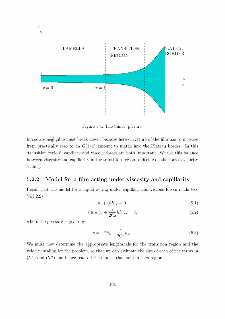
TRANSITION
REGION
PLATEAUBORDER
x
y
LAMELLA
x = 0 x = 1
Figure 5.4: The ‘inner’ picture.
forces are negligible must break down, because here curvature of the film has to increase
from practically zero to an O(1/a) amount to match into the Plateau border. In this
‘transition region’, capillary and viscous forces are both important. We use this balance
between viscosity and capillarity in the transition region to decide on the correct velocity
scaling.
5.2.2 Model for a film acting under viscosity and capillarity
Recall that the model for a liquid acting under capillary and viscous forces reads (see
§4.3.2.2)
ht + (uh)x = 0, (5.1)
(4hux)x +ε
2Cahhxxx = 0, (5.2)
where the pressure is given by
p = −2ux −ε
2Cahxx. (5.3)
We must now determine the appropriate lengthscale for the transition region and the
velocity scaling for the problem, so that we can estimate the size of each of the terms in
(5.1) and (5.2) and hence read off the models that hold in each region.
104

5.2.3 Lengthscale of the transition region and velocity scalings
We find the lengthscale of the transition region from the fact that we must be able to
match this region with both the lamella and the Plateau border. As before, we denote
the radius of curvature of the Plateau border by a. So, dimensionally, we must have
hξξ ∼ 1/a, (5.4)
where ξ is the dimensional lengthscale in the transition region. We nondimensionalise the
transition region thickness with εL (ε is the aspect ratio of the lamella and L is the length
of the lamella), length with δL, and we find εh′ξ′ξ′/(δ2L) ∼ 1/a. We therefore take our
transition region lengthscale to be
δL =√εaL. (5.5)
For example, for typical bubbles with the following characteristic dimensions
ε ∼ 10−3, L ∼ 10−3 m, a ∼ 4× 10⁻⁴ m, (5.6)
we find δ ∼ 0.02. The aspect ratio of the transition region ε′ = ε/δ ∼ 0.05 and so our
thin film models will hold here too.
We have yet to decide on the velocity scaling, U , for this problem. Our transition region is
defined by the fact that viscous and capillary effects balance there, and so this determines
our velocity scaling (found by setting ε′/Ca = 1)
U =γ
µ
√εL
a. (5.7)
For water, µ = 1× 10⁻³ Kg m−1 s−1 and γ = 7× 10⁻² N m−1. We therefore have U ∼ 3.5
m s−1. So we have the inequalities
ε << ε′ = Ca << 1, (5.8)
which imply (i) capillarity is negligible in the lamella; (ii) viscous effects are negligible in
the Plateau border, and (iii) the two effects balance in the transition region, justifying
our initial assumptions.
We read off the model in the lamella from (5.1)-(5.2):
ht + (uh)x = 0, (5.9)
(4hux)x = 0, (5.10)
105

while in the transition region (after performing the scaling x− 1 = δξ) we have
(uh)ξ = 0, (5.11)
(4huξ)ξ +1
2hhξξξ = 0. (5.12)
We note that (5.9)-(5.10) require two boundary conditions on u in order to determine
the solution. One condition is the obvious symmetry condition that the velocity must be
zero at x = 0: the second condition must come from matching with the transition region.
Thus our solution procedure in this case is to consider the transition region first, so as to
find the rate at which liquid leaves the lamella. We shall then return to solve the lamella
problem.
5.2.4 Transition region
We must couple equations (5.11) and (5.12) with boundary conditions at both the lamella
and the Plateau border ends of the region. We set constant velocity and thickness at the
lamella end and match curvature at the Plateau border end:
u→ Q
h0, h→ h0 as ξ → −∞ (5.13)
hξξ → 1 as ξ →∞, (5.14)
where Q is the flux from the lamella into the Plateau border, which is to be found.
Equation (5.11) implies that the flux is uniform through the transition region
uh = Q. (5.15)
Then (5.12) becomes an ordinary differential equation for h, with Q as a parameter. Cru-
cially, the boundary conditions (5.13) and (5.14) overdetermine the problem; integration
of this ordinary differential equation gives rise to a relationship between Q and h0:
Q(h0) =3√
2h320
16. (5.16)
We note that, as the film thins, the flux decreases.
With Q given by (5.16) the transition region model becomes
hhξ =√
2(h
32 − 1
), (5.17)
where h = h/h0 and ξ = ξ/h120 . The solution to (5.17) is
2√h− 2√
3arctan
[1 + 2
√h√
3
]+
1
3log
[1− 2
√h+ h
1 +√h+ h
]=√
2ξ, (5.18)
106

-6 -4 -2 2xi
2
4
6
8
10
h
Figure 5.5: Transition region shape.
where the constant of integration (corresponding to translation in ξ) has been set to zero
without loss of generality. A plot of the solution is given in Figure 5.5. We note that the
profile is monotonic increasing. Finally, we obtain the pressure in the transition region,
using the scaled form of (5.3) and the solution in (5.17),
p = −1
2+
1
4h32
+1
4h3. (5.19)
A plot of the pressure distribution is shown in Figure 5.6. The pressure decreases mono-
tonically from zero in the lamella to −1/2 in the Plateau border. It is the large negative
pressure in the Plateau border (compared with the lamella) which drives the flow and
causes the lamella to drain.
5.2.5 Lamella model
We can also solve the lamella model explicitly in this case. In addition to (5.9) and
(5.10), we specify boundary conditions describing the symmetry of the system, the flux
from the lamella into the Plateau border, and an initial condition to close the model. For
simplicity, we set the thickness of the lamella to be initially uniform. We take
u = 0 at x = 0, (5.20)
u =Q(h)
h=
3√
2
16h
12 at x = 1, (5.21)
h = 1 at t = 0. (5.22)
107

-6 -4 -2 2xi
-0.5
-0.4
-0.3
-0.2
-0.1
p
Figure 5.6: Transition region pressure profile.
Under our assumption that the film thickness is spatially uniform initially, we can easily
see that it remains so. Then we find that
u =3√
2
16h
12x, (5.23)
and (5.9) provides us with an equation for h
ht +3√
2
16h
32 = 0, (5.24)
which has the solution
h =
(1 +
3√
2
32t
)−2
. (5.25)
The solution for h given in (5.25) does not tend to zero in finite time. Hence, as noted in
Chapter 1, we assume that there is a critical thickness (which is a material property of
the film) at which the lamella ruptures. Redimensionalising, we find the lamella lifetime,
depending on the critical rupture thickness hcritD ,
tcritD =
32µL√a
3√
2γ
[(1
hcritD
) 12
−(
1
h∗D
) 12
], (5.26)
where the subscript ‘D’ denotes dimensional quantities, and h∗D is the initial dimensional
lamella thickness. If we use suitable values for the parameters, and suppose the film
starts with thickness 1µm and ruptures when the thickness reaches 0.1µm, then the time
to rupture is tcritD ∼ 4 × 10⁻³ s. Clearly, for foam with a lifetime of many seconds or
108

minutes, the presence of a surfactant or volatile component must alter the dominant
balance so as to slow down drainage significantly.
5.2.6 Implications
In this section we have shown how, in a simple case, we can describe the drainage of a
lamella into a Plateau border by introducing a transition region between the two in which
there are significant curvature changes. In the following sections, we perform a similar
decomposition of the liquid domain for cases in which there is surfactant present in the
system.
5.3 Evolution of films stabilised by a well-mixed sol-
uble surfactant
We apply an analagous procedure to the case where there is a well-mixed soluble surfactant
which is transported by bulk convection, diffusion and surface convection. The general
equations for such a system were derived in §4.5.1.1 and to choose the correct leading-
order model we must decide on our choice of C∗, Γ∗, and ∆γ. To proceed, we make
the assumption that the concentration in the Plateau border is constant, CPb say, on the
time-scale of our lamella drainage problem. We justify this assumption in §5.3.2 later.
We make the further assumption that CPb is small and we set C∗ = CPb. This simplifies
the problem greatly because it allows us to replace the Langmuir isotherm (4.170) with a
linear relation, Γ = ηC (where η = Γ∞/k2), known as the Henry isotherm. We recall that
we performed a similar linearisation of the Langmuir isotherm in Chapter 3. We are also
able to linearise the Frumkin equation (4.169) in this limit too. We choose Γ and ∆γ to
remove the constants of proportionality in the Henry isotherm and in the relation between
surface tension and the surface concentration, and hence Γ∗ = ηCPb and ∆γ = RTηCPb.
We include capillary, Marangoni, viscous, diffusive, convective and replenishing effects in
the model. We therefore have (see the summary at the end of Chapter 4)
ht + (uh)x = 0, (5.27)
(4hux)x +ε
2Cahhxxx +
2Ma
εσx = 0, (5.28)
(hCx)x − Peh (Ct + uCx)−2
Sε(Γt + (usΓ)x) = 0, (5.29)
109

where
u = u+ε3
4Cahxxx
(−y2 +
1
12h2
), (5.30)
us = u− ε3
24Cah2hxxx, (5.31)
p = −2ux −ε
2Cahxx, (5.32)
Γ = C, (5.33)
σx = −Γx. (5.34)
5.3.1 Selection of velocity scale
Again, there are numerous ways that we could select our velocity scale in this case.
However, we make the observation that, for velocities of practical interest (O(10−3) m
s−1 say) the reduced capillary number (Ca/ε) is small and so viscous forces are negligible
everywhere. With small capillary number we have a capillary-static Plateau border, and,
since the curvature of the lamella is small, we conclude that the lamella must be dominated
by Marangoni forces. Our transition region in this case is therefore where the capillary and
Marangoni terms balance. However, we are unable to obtain a velocity scaling from such
a balance, since the remaining dimensionless group in (5.28), T = CaMa/ε2 = ∆γ/(ε2γ)
is independent of the velocity scale chosen.
To ensure a balance in (5.28), we must have a gradient in Γ, which means that we must
ensure that there is a nontrivial balance in (5.29). We choose to balance the surface
convection and bulk diffusion in the transition region, i.e., we set
Sε
δ= 1, so U =
D
η
√εL
a. (5.35)
If we have chosen the velocity scaling inappropriately, we will find that one of remaining
parameters in the system is large and deduce that a different scaling for U is more appro-
priate (as we find in §5.4 for a lamella stabilised by CTAB). For the moment, we choose
to work with an artificial highly diffusive surfactant, with say D ∼ 2× 10⁻⁸ m2 s−1, and
η ∼ 1 × 10⁻⁵ m. We estimate U ∼ 1 × 10⁻⁴ m s−1 (we note that this is much smaller
than the velocity scaling of the previous section), the reduced Peclet number, P = δPe
is O(1), Ca ∼ 10−6, and T = T/δ2 ∼ O(1).
Thus the leading-order model that holds in the lamella is
ht + (uh)x = 0, (5.36)
110

σx = 0, (5.37)
PhCt + 2Γt + PuhCx + 2(usΓ)x = 0, (5.38)
u = us = u, (5.39)
Γ = C, (5.40)
σx = −Γx, (5.41)
while in the transition region we have
(uh)ξ = 0, (5.42)
hhξξξ + T σξ = 0, (5.43)
(hCξ)ξ −PhuCξ − 2 (usΓ)ξ = 0, (5.44)
us = u− βh2hξξξ, (5.45)
Γ = C, (5.46)
σξ = −Γξ, (5.47)
where T = 4a∆γ/(γLε) and β = ε′3/24Ca. In both the lamella and the transition region,
viscous forces are negligible at leading order and the physical structure of the problem is
different from the pure liquid film considered in the previous section. Here, the flow is
completely governed by what is happening at the free surfaces.
5.3.1.1 Parameter sizes and plan for the rest of this section
We first consider the behaviour of this system of equations by analysing the case where
P and T are both O(1), but the ‘lubrication’ parameter β << 1. We note that these are
assumptions that are not, in general, true. If P << 1 we lose the bulk convection term,
and if P >> 1 we must choose a different velocity scaling, balancing bulk convection with
either diffusion or surface convection. The effect of having a very small or very large Tis that h and C vary over different lengthscales, and we have nested transition regions.
However, assuming P, T ∼ O(1) appears to be the most generic case, where all the terms
have the same influence, and so we proceed under this assumption.
Changing β has a different effect on the model. With β << 1, the flow is everywhere
extensional, but with β ∼ O(1), the velocity in the transition region becomes parabolic.
Using typical values for the parameters, β ∼ 2 and so, after considering the (simpler)
β << 1 case, we incorporate the effect of β ∼ O(1) in §5.3.7.
111

We follow the following plan in the rest of this section. First we consider the Plateau
border, and show that our assumptions about the concentration are correct and that its
shape is governed by capillary statics. Next, we consider the problem in the lamella, with
the aim of relating the concentration in the lamella to its thickness. Following this, we
work with the transition region model, using the information already obtained from the
lamella and the Plateau border. As in the last section, the aim will be to find the flux of
liquid, Q, flowing out from the lamella as a function of lamella thickness h0. Finally, we
return to the lamella problem to find how the thickness varies with time, and, ultimately,
the time to rupture. Once this is completed, we consider how the inclusion of a nonzero
β modifies the problem, and we repeat the transition region analysis to find Q(h0) and
then the time to rupture.
5.3.2 Plateau border
In this subsection we justify our assumption that the surfactant concentration is constant
in the Plateau border. To do this, we consider the flux of surfactant leaving the lamella,
which is controlled by surface and bulk convection, and reads, in dimensional variables,
Flux out = huCl
(1 + 2
η
h
), (5.48)
where Cl is the concentration in the lamella. We equate this to the flux into the Plateau
border, sodCPb
dt∼ huCl
a2
(1 + 2
η
h
). (5.49)
We nondimensionalise in the standard way, to get
dCPbdt∼ εL2
a2QCl
(1 +
2η
εLh
). (5.50)
Using typical parameter values, we find that dCPb/dt ∼ 10−1QCl, and we conclude that,
providing Q ∼ O(1) or smaller, CPb is constant on the timescale for lamella drainage.
As noted earlier, with the velocity scaling given by (5.35), Ca ∼ O(10−6) and so our
assumption that the Plateau border is dominated by capillary statics is verified, and the
Plateau border free surfaces have constant curvature 1/a.
5.3.3 Lamella model
The lamella model (5.36)-(5.41) may be simplified to read
ht + (uh)x = 0, (5.51)
Cx = 0, (5.52)
112

(2 + Ph)Ct + PuhCx + 2 (uxC) = 0, (5.53)
where, since capillary forces are small in this region, u = u = us. We note that (5.52)
dictates that C = C(t). So, (5.53) reduces to the following (linear) equation for C,
C = − 2Cux2 + Ph. (5.54)
We impose the boundary conditions of no flux and symmetry at the lamella’s middle,
flux conservation with the transition region, and, for simplicity, that the concentration of
surfactant and the lamella thickness are both constant initially (the concentration must
necessarily be constant at t = 0 to satisfy (5.52). If the concentration is not constant,
we must consider a problem on a shorter timescale than L/U in which the concentration
adjusts), i.e.
u = 0 at x = 0, (5.55)
u =Q
hat x = 1, (5.56)
C = CI , h = 1 at t = 0. (5.57)
As before, Q is the flux of liquid flowing from the lamella into the transition region, and CI
is the initial lamella concentration. The choice of appropriate CI depends on the “history”
of the lamella. Consider the initial formation of the foam as a whole. At the start, the
bubbles are almost spherical, with surfactant distributed uniformly. The liquid drains
through the foam to form the lamella-Plateau border structure. The concentration of
surfactant in the lamella is decreased by the increase in surface area required to generate
this evolution of morphology. Therefore, we conjecture that CI < 1 for draining foams
(in dimensional terms, this reads CI < CPb). However, in some laboratory experiments
to study single lamellae (see Joye et al. [43]), individual thin films are generated by
dipping a ring into surfactant solution. The thin films are automatically forced into
the lamella-Plateau border shape although the concentration of surfactant may still be
assumed uniform. We therefore allow ourselves to consider CI ≤ 1.
We may then solve the system for C to give
C = CI(2 + P)h
2 + Ph . (5.58)
We note that the flux of surfactant from the lamella is given by
Flux = QC
(P +
2
h
), (5.59)
and so we see that, as the film thins, the transport of surfactant is dominated by surface
convection.
113

As in §5.2, we can also solve for u,
u =Q(h)x
h, (5.60)
and finally h is given by ∫ 1
h
dHQ(H)
= t. (5.61)
We return to evaluate this integral once we have determined the flux Q as a function of
thickness using the transition region model.
5.3.4 Transition region
We couple (5.42)-(5.47) with boundary conditions that the film thickness, liquid velocity
and concentration are constant in the lamella. We read off these values from the lamella
model, given the thickness h0, and they are
h→ h0, u→ Q
h0
, C → C0 = CI(2 + P)h0
2 + Ph0
as ξ → −∞. (5.62)
We also match curvature of the film and concentration with the Plateau border and we
set
hξξ → 1, C → 1 as ξ →∞. (5.63)
The corresponding leading-order equations for the liquid velocity, lamella thickness and
concentration of surfactant are
uh = Q, (5.64)
T (C − C0) = hhξξ −h2ξ
2, (5.65)
hCξ = PQ (C − C0) + 2Q
(C
h− C0
h0
), (5.66)
We note that the flow in the transition region is quasi-steady. The first of these equations
is the integrated conservation of mass equation, the second is the integrated longitudinal
force balance, and the third is the integrated surfactant concentration equation. The
constants of integration were found by applying the conditions as ξ → −∞. We note that
(5.65) and (5.66) decouple from (5.64): we can solve for C and h and then read off u from
(5.64).
114

5.3.4.1 Asymptotic behaviour of solutions at ±∞
We must check that the boundary conditions that we wish to impose on (5.65)-(5.66) do
not over-determine the problem. We first reduce the number of parameters in the problem
by setting C = (C − C0)/C0, h = h/h0 and ξ =√T C0/h2
0ξ. The resulting system of
equations for C and h are
C = hhξξ −hξ
2
2, (5.67)
hCξ = ΥQ∗C +Q∗
(C+1
h− 1
), (5.68)
where Υ = Ph0/2 and Q∗ = 2Q/(h0
√T C0) and the boundary conditions that we wish
to impose now read C → 0, h → 1 as ξ → −∞, hξξ → h0/(T C0), C → (1 − C0)/C0
as ξ → ∞. Our plan is to find the behaviour of h and C as ξ → ±∞ and then see
how many of the number of degrees of freedom the boundary conditions eliminate. We
linearise about h ∼ a1ξ2/2 as ξ →∞ by setting
h ∼ a1ξ2
2+ a2ξ + a3 +
a4
ξ+a5
ξ2+O
(1
ξ3
). (5.69)
We note that, in general, we must also look for terms of the form ξme−aξn, but it is
easy to show that these terms do not appear. We find the corresponding form for C by
substituting this into (5.67):
C ∼ a1a3 −a2
2
2+
3a1a4
ξ+
3a2a4 + 6a1a5
ξ2+O
(1
ξ3
). (5.70)
We are able to find relationships between the coefficients in these expansions using (5.68),
and we get the leading order balance
−3
2a2
1a4 = ΥQ∗(a1a3 −
a22
2
)−Q∗. (5.71)
Imposing the boundary conditions as ξ → ∞, we see, trivially, that a1 = h0/(T C0) and
that we must also take a1a3 − a22/2 = (1−C0)/C0 (from (5.70)). Substituting into (5.71)
gives an expression for a4:
a4 = −2T 2C20
3h20
(ΥQ∗
(1− C0
C0
)−Q∗
), (5.72)
and we can generate a5 from (5.68),
a5 =2T 3C3
0
3h30
(ΥQ∗
(1− C0
C0
)−Q∗
)(a2 +
Q∗Υ
2
). (5.73)
115

Since the system exhibits translational invariance, we may set a2 = 0. We can see that
once this is done, a1, a3 . . . are all determined uniquely by (5.67) and (5.68) and the
boundary conditions. We re-write these expansions in the original variables, and they
then read (with error O(1/ξ3))
h ∼ ξ2
2+
(1− CI(2 + P)h0
2 + Ph0
)T + 2 (−P + CI(2 + P))
QT3ξ− (−P + CI(2 + P))
PT Q2
3ξ2,
(5.74)
C ∼ 1 + 2 (−P + CI(2 + P))Q
ξ− 2 (−P + CI(2 + P))
PQ2
ξ2. (5.75)
We note that, for CI = P/(2 +P), the coefficients of the small terms in these expansions
vanish, and that, for CI < P/(2+P), C → 1 from below, while if CI > P/(2+P), C → 1
from above.
We conclude that, for a given set of parameters including the unknown h0 and Q, there
is a unique solution (up to translation) leaving ξ =∞.
At the other end of the range, we linearise about h = 1, setting h ∼ 1+aeλξ. Substituting
this into (5.67) gives
C ∼ aλ2eλξ, (5.76)
and we obtain an equation for λ by substituting into (5.68):
λ3 − (Υ + 1)Q∗λ2 +Q∗ = 0. (5.77)
Setting χ = λ√
1 + Υ, and q = Q∗(1 + Υ)32 , the cubic can be simplified to
χ3 − qχ2 + q = 0. (5.78)
Now the structure of the solution depends on the sign of Q∗. Motivated by the purely
viscous calculation of §5.2, and on physical grounds, we anticipate that Q∗ should be
positive, i.e. the liquid should flow from the lamella into the Plateau border. Therefore we
assume that q > 0 and deduce that (5.78) has at least one negative real root, χ = −χ∗(q)say, where
χ∗ = −q3
+2
13 q2
3f(q)+f(q)
213 3, (5.79)
and
f(q) =(
27q − 2q3 + 3√
3q√
27− 4q2) 1
3
. (5.80)
The other two roots are, in terms of χ∗,
χ± =χ∗
2(1− χ∗2)
(1±
√4χ∗2 − 3
), (5.81)
116

which are real if χ∗ >√
3/2 and form a conjugate pair with positive real part if χ∗ <√
3/2.
The corresponding behaviour for h and C is monotonic decay in the former case and
oscillatory decay in the latter.
The corresponding condition on q for oscillatory behaviour reads
q =2Q
h0
√TC0
(1 +Ph0
2
) 32
<3√
3
2. (5.82)
and using (5.62), this condition reads
B =4√
2Q(1 + Ph0
2
)2
3√
3√T CI(2 + P)h
320
< 1. (5.83)
So, as we approach −∞, we find that we must suppress one growing mode (the one given
by χ = −χ∗), and the other two modes decay either monotonically or in an oscillating
fashion, as dictated by (5.83). In either case, for a given set of parameters (including h0
and Q), there is a one-parameter family of solutions leaving ξ = −∞ (as in Tuck and
Schwartz [75]) of the form
h ∼ 1 + α(eξχ− + eξχ+
), (5.84)
where α is a free parameter and translational invariance has been used to make the
coefficients of the two exponentials the same.
We consider two possible numerical procedures for solving the problem. One alternative
is to start from ξ = −∞ (in practice, some large negative value), in which case we have
two shooting parameters, α (c.f. (5.84)) and Q to vary, and two conditions hξξ → h0/T C0
and C → (1−C0)/C0 to satisfy as ξ →∞. Thus it is at least plausible that the problem
is well posed and that Q is uniquely determined. The method that we prefer to employ,
however, is to start from ξ = ∞ (again, really a large positive value), in which case we
only have one free parameter Q, which we vary in order to satisfy h→ 1 as ξ → −∞.
We note that, since Q is not known a priori, we are not able, given a set of parameters,
to decide whether or not we would expect oscillating solutions before attempting the
numerical solution.
5.3.5 Summary
We summarise the results presented above before obtaining numerical solutions of the
transition region model.
117

• There is a relationship between the concentration and thickness in the lamella which
reads
C0 = CI(2 + P)h0
2 + Ph0
. (5.85)
• The behaviour at the Plateau border end of the transition region depends on the
size of
K =P
(2 + P)CI. (5.86)
This condition does not depend on h0 or Q. If K > 1, then C → 1 from below. If
K < 1, we have C → 1 from above, and since the concentration in the lamella is less
than that in the Plateau border (except possibly at t = 0), we must have Cξ = 0
somewhere, and hence C must be nonmonotonic.
• The behaviour at the lamella end of the transition region is determined by the size
of
B =4√
2Q(1 + Ph0
2
)2
3√
3√T CI(2 + P)h
320
. (5.87)
If B < 1, we expect oscillating solutions as we approach the lamella. If B > 1, we
expect monotonic behaviour as we approach the lamella.
• We appear to have a well-posed system which, upon numerical solution, will yield
the flux Q for each given value of h0, P ,T and CI . Our plan is to solve for Q(h0)
with all the other parameters fixed, and then find the evolution of the lamella using
(5.61).
The flow of information is shown in Figure 5.7. The arrows show how the information is
transmitted between the regions, and shows that we pass information about the surfactant
concentration into the transition region from both the lamella and the Plateau border,
and we pass information about the liquid from the Plateau border into the transition
region and then into the lamella.
5.3.6 Results and discussion
We solve the transition region system (5.65)-(5.66) to obtain Q = Q(h0). To demonstrate
two classes of solutions to the transition region model, we start by keeping h0, P and Tfixed while varying CI . First, we use h0 = 0.8, P = 5, T = 5, CI = 0.5, and we find
that Q = 0.4292. We calculate B = 1.405 > 1, and so we expect monotonic behaviour as
ξ → −∞. We also have K > 1 , and so expect C → 1 from below as ξ → ∞. The film
thickness and surfactant concentrations are shown in Figure 5.8. They exhibit monotonic
increase in both h and C, as predicted. We call such solutions ‘monotonic’. Secondly, we
118

Concentration
PlateauBorder
TransitionLamella Region
Solve for giventhickness to
find flux
Concentration
Flux Curvature
Figure 5.7: Flowchart showing information routes.
set CI = 1, and we find that Q = 0.0349. We calculate B = 0.0808 < 1, and so we expect
the solution to oscillate as we approach −∞. We also have K < 1 and so we expect
C → 1 from above as ξ →∞. The film thickness and concentration of surfactant in this
case are shown in Figure 5.9. Both the film thickness and the surfactant concentration
are nonmonotonic, as expected. We call such solutions ‘dimpled’.
We show plots of the surface convective flux 2QC/h, bulk convective flux PQC and the
diffusive flux −hCξ when h0 = 0.8, P = 5, T = 5, and CI = 0.5 in Figure 5.10. We
see that the diffusive flux is always negative, i.e., diffusion transports surfactant from
the Plateau border into the lamella, and that the convective fluxes are both positive,
indicating that they transport surfactant from the lamella to the Plateau border. We
note that bulk convection appears to be the dominant mechanism.
We repeat this procedure for the same parameters but setting CI = 1, and we show
the results in Figure 5.11. Here, bulk convection and surface convection again transport
surfactant from the lamella into the Plateau border, but now transport by diffusion is
more complicated. We remember that the concentration profile in this parameter regime
is nonnomotonic, and that the concentration achieves a maximum within the transition
region. We see that diffusion transports surfactant out from this maximum (both towards
the Plateau border and further into the transition region).
119

-10 -5 5 10xi
1.5
2
2.5
h
-10 -5 5 10 15 20xi
0.6
0.7
0.8
0.9
C
Figure 5.8: Results for thickness and concentration in a monotonic solution.
120

-10 -5 5 10xi
0.6
0.7
0.8
0.9
1.1
1.2
h
-10 -5 5 10xi
0.92
0.94
0.96
0.98
1.02
1.04
C
Figure 5.9: Results for thickness and concentration in a dimpled solution.
121
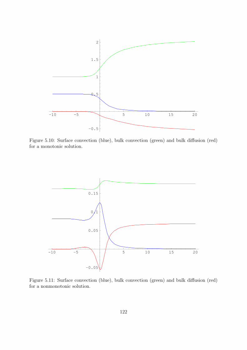
-10 -5 5 10 15 20
-0.5
0.5
1
1.5
2
Figure 5.10: Surface convection (blue), bulk convection (green) and bulk diffusion (red)for a monotonic solution.
-10 -5 5 10 15 20
-0.05
0.05
0.1
0.15
Figure 5.11: Surface convection (blue), bulk convection (green) and bulk diffusion (red)for a nonmonotonic solution.
122

We may examine the behaviour of each of these mechanisms for large ξ by substituting
the appropriate expansions from §5.3.4.1. We find
PQC ∼ PQ+ 2P(−P + CI(2 + P))Q2
ξ+O
(1
ξ2
), (5.88)
2QC
h∼ 4Q
ξ2+O
(1
ξ2
), (5.89)
−hCξ ∼ −(−P + CI(2 + P))Q+ 2(−P + CI(2 + P))PQ2
ξ+O
(1
ξ2
), (5.90)
i.e., as ξ →∞, the bulk convection term tends to the constant PQ from below if K > 1,
the surface convection term always tends to zero from above, and the diffusion term tends
to the constant (−P + CI(2 + P)) which is negative if K > 1. These behaviours are
supported by the numerical solutions above.
We now calculate the pressure in the transition region using
p = −1
2hxx. (5.91)
As we would expect, in a monotonic solution, shown in red in Figure 5.12, we see that the
pressure decreases monotonically from 0 to −1/2. In a dimpled solution, shown in blue
in Figure 5.12, we see that the pressure variation is non-monotonic.
-10 -5 5 10xi
-0.5
-0.4
-0.3
-0.2
-0.1
p
Figure 5.12: Pressure in a monotonic solution (red) and a dimpled solution (blue).
123

profilePressure
21
Plateau borderP > P0P0 Ps
LamellaContraction
Border
Figure 5.13: Barigou and Davidson’s rejected transition region.
Notice that in the latter case there is a maximum of pressure in the transition region,
i.e., the pressure increases to a value greater than zero before a sudden decrease to a
value just below −1/2. The pressure then tends to −1/2 from below. We compare this
pressure distribution with that dismissed by Barigou and Davidson [5], shown in Figure
5.13. Since they have a sharp change in boundary structure at the start of the transition
region (a change from a stress-free boundary in the lamella to a ‘no-slip’ boundary in the
transition region), they have a ‘step rise in pressure’ at the ‘inlet to the contraction zone’.
It is this step that they reject as unphysical. Our results have a gradual change in stress
at the surface and we obtain a smooth profile for the pressure when we have a dimpled
solution. We therefore see no reason to reject this type of solution on the basis of the
pressure profile.
We now generate Q = Q(h0) for a given set of parameters. We take P = 0.5, T = 0.5,
CI = 0.1, and we vary h0 from 1 to 0.1 (to tie in with the initial and critical values used
in §5.2 earlier). Here, we have K > 1, and so we expect C → 1 from below as ξ → ∞.
The variation is shown in Figure 5.14. Surprisingly, the flux increases as h0 decreases, in
contrast with the surfactant-free case.
We show the thickness of the transition region for h0 between 0.1 and 1 (using these
parameters) in Figure 5.15, and we show some of the corresponding concentrations in
Figure 5.16. These may be thought of as “time snapshots” of the transition region as
the lamella drains from h = 1 to h = 0.1. We calculate B for each of the snapshots. We
find that, for h0 = 0.6 and larger, we have B < 1, while for the other solutions, we have
124

0.2 0.4 0.6 0.8 1h0
0.08
0.12
0.14
Q
Figure 5.14: Graph showing Q as a function of h0 for P = 0.5, T = 0.5, CI = 0.1.
-30 -20 -10 10xi
0.25
0.5
0.75
1
1.25
1.5
1.75
h
Figure 5.15: Transition region thickness for various values of h0, with P = 0.5, T = 0.5,CI = 0.1.
B > 1. If we examine the solutions closely for large negative ξ, we see that the solutions
agree with this prediction. We note that condition (5.87) for oscillatory solutions contains
the factor Q/h320 , and that this factor increases as h0 decreases, with the flux as shown in
Figure 5.14. Hence, (5.87) dictates that the oscillations as ξ → −∞ die away as the film
125
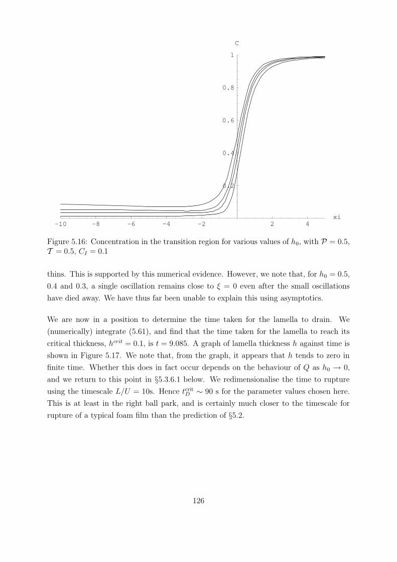
-10 -8 -6 -4 -2 2 4xi
0.2
0.4
0.6
0.8
1
C
Figure 5.16: Concentration in the transition region for various values of h0, with P = 0.5,T = 0.5, CI = 0.1
thins. This is supported by this numerical evidence. However, we note that, for h0 = 0.5,
0.4 and 0.3, a single oscillation remains close to ξ = 0 even after the small oscillations
have died away. We have thus far been unable to explain this using asymptotics.
We are now in a position to determine the time taken for the lamella to drain. We
(numerically) integrate (5.61), and find that the time taken for the lamella to reach its
critical thickness, hcrit = 0.1, is t = 9.085. A graph of lamella thickness h against time is
shown in Figure 5.17. We note that, from the graph, it appears that h tends to zero in
finite time. Whether this does in fact occur depends on the behaviour of Q as h0 → 0,
and we return to this point in §5.3.6.1 below. We redimensionalise the time to rupture
using the timescale L/U = 10s. Hence tcritD ∼ 90 s for the parameter values chosen here.
This is at least in the right ball park, and is certainly much closer to the timescale for
rupture of a typical foam film than the prediction of §5.2.
126

2 4 6 8t
0.2
0.4
0.6
0.8
1
h
Figure 5.17: Graph showing lamella thickness versus time for P = 0.5, T = 0.5, andCI = 0.1.
5.3.6.1 Unexpected results
While attempting numerical solutions to the transition region model, we found the fol-
lowing surprising behaviour. We noticed that, for some parameter regimes, Q appears to
tend to infinity at a finite value of h0. We illustrate such behaviour in the case when we
have CI = 0.5, P = 5, and T = 5, shown in Figure 5.18. We were unable to find a value
of Q for h0 ≤ 0.58. At first, we dismissed these results as erroneous, but such behaviour
can in fact be justified asymptotically. For convenience, we combine (5.65) and (5.66) to
eliminate C, giving
h3h′′′ = Q(Ph+ 2)
(hh′′ − 1
2h′
2
)+ 2QT C0
(1− h
h0
), (5.92)
with
h→ h0 as ξ → −∞, (5.93)
h ∼ 1
2ξ2 + T (1− C0) as ξ →∞. (5.94)
We then reduce the order of the problem by setting h′2 = G(h). (Note that the solutions
of interest here are all monotonic, so there is no problem defining G(h)). The problem
becomes √GGhh =
Q
h3(2 + Ph) (hGh −G) +
4QT C0
h3
(1− h
h0
), (5.95)
where
G(h0) = 0, G′(h0) = 0, (5.96)
127

0.6 0.7 0.8 0.9h0
2.5
5
7.5
10
12.5
15
17.5
Q
Figure 5.18: Graph showing Q against h0 for CI = 0.5, P = 5, and T = 5.
G ∼ 2h− 2T (1− C0) as h→∞. (5.97)
In our earlier approach, we varied h0 and found the corresponding value for Q. Here, we
use the opposite idea, i.e., we let Q→∞, and see if we can deduce a value for h0.
First, we consider the problem near to the Plateau border. We note that (5.95) is singular
as Q→∞, i.e., to lowest order the highest derivative disappears. However, as h becomes
large to match with the Plateau border this term comes back in at leading order. The
appropriate scaling is h = Q2h, G = Q2G, and we arrive at
h3√GGhh =
(Ph+
2
Q2
)(hGh − G) +
4T C0
Q2
(1
Q2− h
h0
), (5.98)
with
G ∼ 2h− 2T (1− C0)
Q2as h→∞. (5.99)
We seek an outer solution as an asymptotic expansion in powers of 1/Q2, and the leading-
order problem reads
h3√G0G0hh =
1
2Ph(hG0h −G0). (5.100)
It is fortunate that we can spot a solution to (5.100) which also satisfies the boundary
condition as h→∞, namely
G0 = 2h. (5.101)
128

We need not look for a more general solution since we have already established that the
solution eminating from ∞ is unique. Comparing terms of O(1/Q2), we find
√2hG1hh =
Ph2
(hG1h −G1)− 4T C0
h0h2. (5.102)
This has the solution
G1 =1
2P2
(h
(α1 −
√2P(α1 − α2)√
he−√
2P√h + (α2 − α1)e
−√
2P√h
))− 4T C0
Ph0
. (5.103)
We want G1 ∼ −2T (1− C0) as h→∞, so we set α2 = 0, and
α1 =8T C0
Ph0− 4T (1− C0). (5.104)
Therefore G reads
G ∼ 2h+1
P2Q2
(8T C0
Ph0
− 4T (1− C0)
)(h− (h+ P
√2h)e
−q
2
hP)− 4T C0
Ph0Q2+O
(1
Q4
).
(5.105)
We obtain a matching condition for the inner problem by susbtituting G = G/Q2, h =
h/Q2 and thus the two-term outer expansion of the two-term inner solution must read
G ∼ −4T C0
Ph0
+ 2h+
(8T C0
h0P3Q2− 4T (1− C0)
P2Q2
)h, (5.106)
as h→∞.
We now consider (5.95) in the limit Q → ∞. We seek an asymptotic solution in powers
of 1/Q, and the leading-order equation reads
hGh −G+4T C0
(2 + Ph)
(1− h
h0
)= 0, (5.107)
which has the solution
G = αh+1
4h0
[8T C0h0 + (8T C0 + 4T C0h0P)h log
(h
2 + Ph
)]. (5.108)
Applying the matching condition (5.106) at leading-order, we obtain
G = 2h
[1 +
CI(2 + P)T2
log
( Ph2 + Ph
)]+
2T CI(2 + P)h0
2 + Ph0
. (5.109)
We remember that here we are trying to find h0 as a function of Q (in the limit as Q→∞)
and to do so we apply the left-hand boundary conditions G(h0) = 0 and G′(h0) = 0. We
set
h0 = hc +hc1Q
+hc2Q2
+ . . . , (5.110)
129

so that hc is the value of h0 (if it exists) at which Q approaches infinity, and satisfies
G(hc) = 0, i.e.
2hc
[1 +
CIT (2 + P)
2log
( Phc2 + Phc
)]+
2T CI(2 + P)hc2 + Phc
= 0. (5.111)
For given CI , P and T , (5.111) has two nonnegative solutions for hc, one of which is
hc = 0. However, this can be rejected since one can readily show that G′(0) 6= 0. The
other, positive, solution for hc does satisfy G′(hc) = 0. For T = 5, P = 5, and CI = 0.5,
this gives hc = 0.587. So, our numerical observations that Q → ∞ for h0 around 0.59
appear to have been justified. With T = 0.5, P = 0.5, and CI = 0.1, we calculate
hc = 4.4× 10⁻⁷. Clearly, in our calculations we did not make h0 small enough to notice
the presence of this hc. We note that the existence of hc, however small, explains why the
flux increases as h0 decreases.
In general, the positive solution of (5.111) can be written as
hc = Phc = F (T ∗), (5.112)
where T ∗ = CIT (2 + P), and F is given by
T ∗ = − 2(2 + F (T ∗))(2 + F (T ∗)) log
[2+F (T ∗)F (T ∗)
]+ 2
. (5.113)
We show the solution to (5.113) in Figure 5.19. We note that, as T ∗ → 0, F → 0, and
we find that the behaviour is
F ∼ 2e−1− 2T ∗ as T ∗ → 0, (5.114)
and in particular if T ∗ is small, F is exponentially small. This is the reason why we did
not notice the presence of hc when we took CI = 0.1, and T = P = 0.5 earlier. We also
note that, as T ∗ →∞, F →∞, and
F ∼√T ∗ as T ∗ →∞, (5.115)
and so, for large enough T ∗, we are in a situation where hc > 1 (i.e., the critical thickness
is above the starting thickness of the lamella) and we cannot even start to follow the
evolution of h.
Of course, in practice the flux cannot become infinite on physical grounds. We anticipate
that, as Q becomes large, some physical effects that have thus far been neglected become
important. Moreover, these should then describe the behaviour of Q for h < hc. There
130

1 2 3 4Tstar
0.2
0.4
0.6
0.8
1
F
Figure 5.19: Graph showing how the function F varies with T ∗
is more than one candidate for the relevant extra effect; for example, it could be inertia,
but we will only assess the effect of the viscous term that was neglected in (5.43). When
this term is included, the transition region model reads
uh = Q, (5.116)
−νQ(hξh
)
ξ
+ hhξξξ − T Cξ = 0, (5.117)
hCξ = PQ(C − C0) + 2Q
(C
h− C0
h0
), (5.118)
where ν = 8δCa/ε. Using our velocity scaling, ν ∼ 4 × 10⁻⁵ << 1. As previously, we
re-write the problem as one equation for h, which reads
h3h′′′ = Q(2 + Ph)
(hh′′ − 1
2h′2)
+ 2T C0
(1− h
h0
)+ νQ
(h
(h′
h
)′− 2Q
h′
h−PQh′
).
(5.119)
We set G = h′2, and the problem becomes
h3√GGhh=Q(2 +Ph)(hGh−G)+4T QC0
(1− h
h0
)+νQ
(Gh−
2G
h−Q
(4
h+ 2P
)√G
).
(5.120)
We can see that for Q ∼ O(1), we have the problem that we have just considered, but for
Q ∼ O(1/ν) the viscous terms come in and we have the equation
hGh −G+4T C0
2 + Ph
(1− h
h0
)− 2
hQ√G = 0, (5.121)
131

where Q = νQ. We note that Q is the viscous scaled flux that we considered in §5.2.
We hope that the solution to this equation will provide insight into what happens to the
solution after the lamella thickness has reached hc. In any case, since the flux becomes
very large at this thickness, we assume that the rest of the drainage occurs on the (much
faster) viscous timescale, and so the film thins to the rupture thickness very quickly.
We conclude by summarising the behaviour of the solution that we have uncovered in this
subsection.
• We are able to find a solution to the surfactant problem (5.65)-(5.66) providing h0
is larger than a critical value hc given by[1 +
CIT (2 + P)
2log
( Phc2 + Phc
)]+T CI(2 + P)
2 + Phc= 0. (5.122)
• As h0 → hc from above, Q→∞.
• To find the behaviour of solutions once the lamella has thinned to hc, we must
include more physics; we considered introducing the viscous terms. We obtain a
new model that holds when viscous effects are significant.
0.2 0.4 0.6 0.8t
0.2
0.4
0.6
0.8
1
h
with fast velocityLamella drains
Lamella drains with slow velocity
Q→∞
(Viscous forcesbecome important)
Figure 5.20: Schematic showing how the thickness of a lamella changes with time. Theupper part of the curve was calculated for CI = 0.5, P = 5, T = 5.
• We hypothesise that the film thins from hc to hcrit on the fast viscous timescale and
we show a schematic of our conjecture for the variation of the film thickness with
time in Figure 5.20.
132

We conjecture that if hc > 1, the surfactant is unable to prolong the life of the film, since
for h0 = 1 < hc, we are already in the regime that requires a viscous velocity scaling.
5.3.7 Including the ‘lubrication’ term
We now take into account the effect of nonzero β on the solution. If β = O(1), then the
lamella model remains the same but the transition region model is modified. We have
uh = Q, (5.123)
T (C − C0) = hhξξ −h2ξ
2, (5.124)
(1 + βT C)hCξ = PQ(C − C0) + 2Q
(C
h− C0
h0
), (5.125)
where β = 2β, with
hξξ → 1, C → 1, as ξ →∞, (5.126)
h→ h0, u→ Q
h0, C → C0, as ξ → −∞, (5.127)
and
u = u+ 3β
(−y2 +
1
12h2
)hξξξ, (5.128)
C0 =CI(2 + P)
2 + Ph0h0. (5.129)
5.3.7.1 Behaviour as ξ → ±∞
In order to check that the problem is well-posed, we must again consider the asymptotic
behaviour of this system. We scale C = C0 +C0C, h = h0h and ξ = h0/√T C0ξ, and the
system of equations becomes
C = hhξξ −h2ξ
2, (5.130)
(1 + β∗ + β∗C
)hCξ = Q∗ΥC +Q∗
(C + 1
h− 1
), (5.131)
where, as before, Υ = Ph0/2, Q∗ = 2Q/(h0
√T C0), and we have the extra parameter
β∗ = βT C0. On substituting
h =a1ξ
2
2+ a2ξ + a3 +
a4
ξ+a5
ξ2+O
(1
ξ3
), (5.132)
(again, we do not explicitly search for exponentially small terms), we find that
C = a1a3 −a2
2
2+
3a1a4
ξ+
3a2a4 + 6a1a5
ξ2+O
(1
ξ3
). (5.133)
133

Using (5.131),
a4 = −2(Q∗Υ
(a1a3 − a2
2
2
)−Q∗
)
3a21
(1 + β∗ + β∗
(a1a3 − a2
2
2
)) , (5.134)
a5 = −a2a4
a1
−
(a4Q∗Υ
2a1+
3a1a24β∗
4
)
1 + β∗ + β∗(a1a3 − a2
2
2
) , (5.135)
which reduce to (5.72) and (5.73) when β∗ is set to zero. Imposing boundary conditions
as ξ →∞, we see that a1 = h0/(T C0) and a1a3 − a22/2 = (1− C0)/C0. Hence, imposing
a2 = 0 by translational invariance, we see that the solution satisfying the conditions at
ξ =∞ is unique.
If we look for stability of h = 1 by substituting h = 1 + aeλξ as ξ → −∞, we obtain
(1 + β∗)λ3 = Q∗(Υ + 1)λ2 −Q∗, (5.136)
as the equation for λ. In this case, we may reduce (5.136) to (5.78) by setting χ = λ√
Υ + 1
and q = Q∗(1 + Υ)32/(1 + β∗). We therefore expect oscillations of the solution as we
approach minus infinity if
2Q(1 + Ph0
2
) 32
h0
√T C0(1 + βT C0)<
3√
3
2, (5.137)
i.e., if
B =4√
2Q(1 + Ph0
2
)2
3√
3h320
√T CI(2 + P)
(1 + βT CI(2+P)h0
2+Ph0
) < 1. (5.138)
We either have two real roots indicating monotonic behaviour or a conjugate pair suggest-
ing oscillatory behaviour as we approach the lamella. Again, we have a one-parameter
family of solutions eminating from ξ = −∞. We conclude that we are not over-specifying
the problem, and that, as before, the most convenient numerical solution procedure is to
start from ξ =∞ and vary Q until h→ 1 as ξ →∞.
5.3.7.2 Surface and centre-line velocities as ξ →∞
We use asymptotics to examine the behaviour of the velocities as we approach the Plateau
border. Scaling h = h0h′, y = h0y
′, ξ = h0/(√T C0)ξ′ and u = (T C0)
32u′, we have
(dropping primes)
u′ =Qh′
+ 3βh′ξ′ξ′ξ′
(1
12h′2 − y′2
), (5.139)
134

where Q = Q/(h0(T C0)32 ). Calling u′cl the velocity of the liquid at the centreline, we have
the following expressions for u′s and u′cl
u′s =Qh′− β
2h′2h′ξ′ξ′ξ′ , (5.140)
u′cl =Qh′
+β
4h′
2h′ξ′ξ′ξ′ . (5.141)
Using (5.69),
u′s ∼3a2
1a4β
4+
3a5a21β
ξ′+
2Qa1
+ β2(6a1a3a4 + 15a2
1a6)
ξ′2+O
(1
ξ′3
), (5.142)
u′cl ∼ −3a2
1a4β
8− 3a5a
21β
2ξ′+
2Qa1− β
4(6a1a3a4 + 15a2
1a6)
ξ′2+O
(1
ξ′3
), (5.143)
and we use the expression for a4 given by (5.72) to decide whether we have u′s > 0, u′cl < 0
or u′s < 0, u′cl > 0 as ξ′ →∞. If we set
D =Ph0
2
(2 + Ph0
CI(2 + P)h0− 1
)− 1 =
2 + Ph0
2(K − 1), (5.144)
then we have u′s > 0 if D < 0 and vice versa, i.e., u′s > 0 if K < 1. In the special case where
CI = P/(2+P) (i.e., K = 1), both a4 and a5 are zero, but a6 = −Q∗T /(h0(1+β∗+ 2β∗
Ph0)) 6=
0. Here, we have u′s, u′cl → 0 as ξ′ →∞, where u′cl always approaches from above and u′s
approaches from above providing
PT (1 + βT )
15β(2 + Ph0)2> 1. (5.145)
5.3.7.3 Summary
In addition to the points raised in §5.3.5, we have
• The condition for oscillating solutions as ξ → −∞ is
B =4√
2Q(1 + Ph0
2
)2
3√
3h320
√T CI(2 + P)
(1 + βT CI(2+P)h0
2+Ph0
) < 1. (5.146)
• The surface velocity is positive as we approach the Plateau border if K < 1, and
the centre-line velocity is negative. If K > 1, then the surface velocity is negative
and the centreline velocity is positive. We therefore expect eddies to be set up at
the entrance to the Plateau border, with direction of rotation being determined by
K.
135

5.3.7.4 Results and discussion
We solve the transition region model and, again, see the two classes of solution. Here, since
the liquid velocity is no longer extensional, we can visualise the flow easily by plotting
the velocity field. To do this, we must use the vertical velocity, which reads,
v =Q
h2hxy − βhxxxx
(h2
4y − y3
)− β
2hhxhxxxy. (5.147)
With T = 5, P = 5, CI = 0.5, h0 = 0.8 and β = 1, we find that Q = 2.008. We calculate
B = 1.97 > 1 and hence we expect no oscillations. We note that, as before, K > 1,
and so we expect that C → 1 from below and that us < 0, ucl > 0 as ξ → ∞. We
show the transition region shape and the velocity field in the region in Figure 5.21 (we
do not show the monotonic increasing concentration profile). We observe a monotonic
solution in which the velocity decreases as the liquid approaches the Plateau border, and
the centre-line velocity is positive while the surface velocity becomes negative. Eddies are
set up at the entrance to the Plateau border which drive liquid down the transition region
walls while returning it along the centre-line.
-4 -2 2 4
-4
-2
2
4
Figure 5.21: Velocity field for a solution where K > 1.
136

-4 -2 2 4
-4
-2
2
4
Figure 5.22: Velocity field for a solution where K < 1.
With T = 5, P = 5, CI = 1.0, h0 = 0.8 and β = 1, we find Q = 0.2095. We calculate
B = 0.086 < 1, predicting oscillations, and since K < 1, we expect that us > 0 and ucl < 0
as ξ → ∞. Plots of the transition region shape, along with velocity field are shown in
Figure 5.22. We observe a dimpled solution in which the velocity decreases in magnitude
as the liquid aproaches the Plateau border, and the velocity beomes negative on the
centre-line, and is always positive along the free surfaces. In contrast to the previous
case, eddies are now set up which send the liquid in the opposite direction, that is, the
liquid moves into the Plateau border along the walls and out along the centreline.
We stress that the cases us > 0, us < 0 are not dependent on whether or not we have a
dimpled solution, but merely on whether K ≷ 1. We examine the effects of increasing the
value of β from zero to one in the two cases we presented earlier. Surface velocities and
the centreline velocities for β = 0 (black), 0.2 (red), 0.4 (green), 0.6 (blue), 0.8 (purple)
and 1.0 (cyan) are shown in Figure 5.23. When β = 0 the liquid velocity is everywhere
positive. With nonzero β, we note that in the K > 1 case (with CI and P fixed), increasing
β from zero creates a stagnation point which travels down the free surface from infinity.
The centreline velocity remains positive everwhere in this case. When K < 1, increasing
β from zero creates a stagnation point on the centreline which travels in from infinity.
137
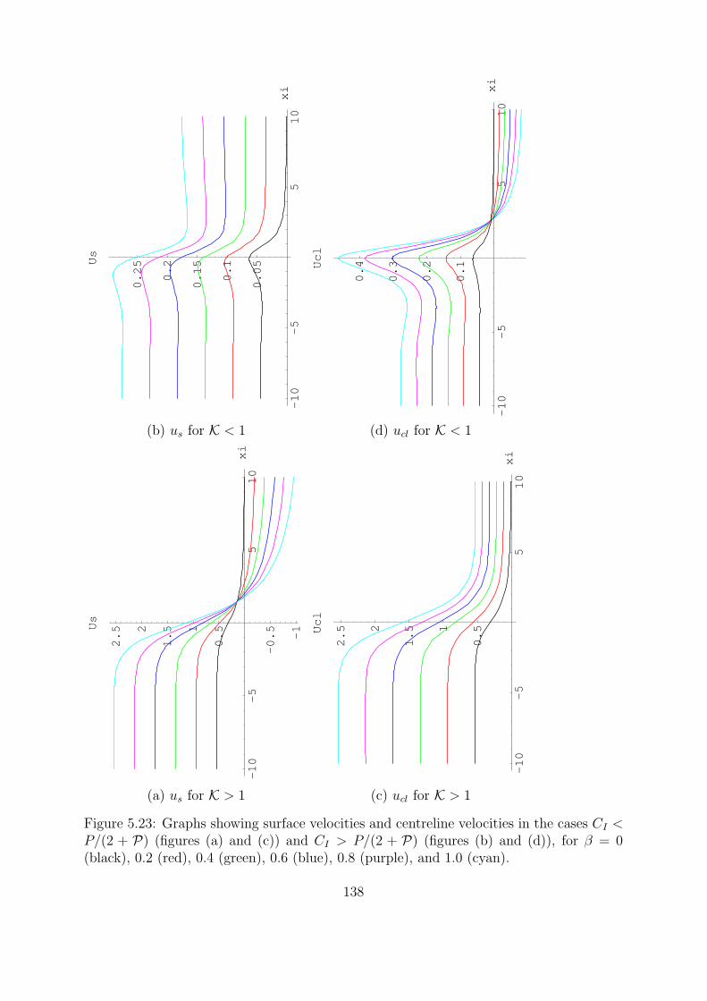
-10
-5
510
xi
0.05
0.1
0.15
0.2
0.25Us
-10
-5
510
xi
0.1
0.2
0.3
0.4Ucl
(b) us for K < 1 (d) ucl for K < 1
-10
-5
510
xi
-1
-0.5
0.51
1.52
2.5Us
-10
-5
510
xi
0.51
1.52
2.5Ucl
(a) us for K > 1 (c) ucl for K > 1
Figure 5.23: Graphs showing surface velocities and centreline velocities in the cases CI <P/(2 + P) (figures (a) and (c)) and CI > P/(2 + P) (figures (b) and (d)), for β = 0(black), 0.2 (red), 0.4 (green), 0.6 (blue), 0.8 (purple), and 1.0 (cyan).
138

The surface velocity remains positive everywhere in this case.
We proceed to generate Q = Q(h0) for a given set of parameters. We take P = 0.5,
T = 0.5, CI = 0.1, and β = 1, and we vary h0 from 1 down to 0.1. The variation of Q
with h0 is shown in Figure 5.24. As previously, we see that Q increases as h0 decreases.
We briefly comment on the behaviour of the solution as Q→∞. In this case, we combine
(5.124)-(5.125) to give
(1 + βT C0 + β
(hh′′ − 1
2h′2))
h3h′′′ = Q(Ph+ 2)
(hh′′ − 1
2h′2)
+ 2QT C0
(1− h
h0
),
(5.148)
and the boundary conditions remain the same, viz (5.93)-(5.94). Here, we do not attempt
to analyse asymptotically this equation in the limit as Q → ∞. Rather, we note that
the condition (5.122) giving hc in the extensional flow case was obtained by considering
the leading-order inner problem in the limit as Q → ∞, and that (5.148) has the same
leading-order behaviour. We therefore have the same condition for hc, namely (5.122).
We note that this is a preliminary result and that we have yet to check that the matching
with the outer problem can be completed without any complications.
Finally, we integrate (5.61), to give h = h(t) as shown in Figure 5.25 and calculate the
time taken for the lamella to reach its critical thickness, which is t = 8.82, which we
redimensionalise to give tcritD = 88 s. Comparing this to the case β = 0, we see that the
inclusion of the parabolic velocity profile has resulted in a slight decrease in the rupture
time. We stress that the main effect of including the lubrication term is that it either
retards the surface flow and accelerates the centre-line flow, or vice versa, depending on
the magnitude of K.
139

0.2 0.4 0.6 0.8 1h0
0.12
0.14
0.16
0.18
0.2
Q
Figure 5.24: Graph showing Q as a function of h0 for P = 0.5, T = 0.5, CI = 0.1, andβ = 1.
1 2 3 4 5 6 7t
0.2
0.4
0.6
0.8
1
h
Figure 5.25: Graph showing lamella thickness with time for P = 0.5, T = 0.5, CI = 0.1and β = 1.0.
140

5.3.8 Conclusions
We present a summary of the important results and behaviour of the solutions that we
have uncovered in this section.
• We identified a relationship between the lamella concentration and thickness, which
we used in the solution of the transition region model.
• In the summary §5.3.5, we presented conditions on two key parameters, K and Bwhich determine the behaviour at the Plateau border end and lamella end of the
transition region respectively, in the case when β = 0. The corresponding conditions
when β ∼ O(1) were given in §5.3.7.3.
• We examined numerical solutions to the transition region model and showed that
they had the behaviour predicted by the key parameters.
• The solutions fall into three categories: monotonic solutions, solutions that are
nonmonotonic but tend monotonically to the lamella thickness, and nonmonotonic
solutions that oscillate as the lamella is approached.
• We obtained the flux of liquid from the lamella into the transition region, as a
function of lamella thickness, for a given set of parameters.
• We solved the lamella model, using this flux, to obtain a time to critical thickness,
which on redimensionalising, was 90 seconds in the β = 0 case, and was slightly
reduced in the β = 1 case.
• We found (numerically) that, for some parameter values, the flux tends to infinity
at a finite lamella thickness. We were able to predict this thickness by considering
the Q → ∞ limit of the model. We conjectured that viscosity enters the model
when Q became sufficiently large, and enables the lamella to carry on thinning.
• We saw that, when β is nonzero, eddies are set up in the transition region which
draw liquid into the Plateau border along the centreline in one case, and along the
free surfaces in another. The size of K determines which scenario occurs.
In the following two sections, we present and solve the models for a lamella stabilised by
CTAB and an insoluble pulmonary surfactant. The methodology used is identical to that
in this section, so we omit the bulk of the details.
141
5.4 Example: evolution of a thin film stabilised by
CTAB
We use the ideas of the previous section to look at drainage of a lamella stabilised by
CTAB. We recall that for CTAB, D ∼ 5 × 10⁻¹⁰ m2 s−1, and if we proceed using the
velocity scaling given in (5.35) we find that U ∼ 2.5×10⁻⁶ m s−1. We calculate Pe ∼ 0.05
but β ∼ 2500. Since ε ∼ 10−3, including such a large β is asymptotically dubious. We
conclude that the velocity used in §5.3 is inappropriate in this case. We note that we
must still have a nontrivial balance in the surfactant equation in the transition region or
we will not have gradients in the concentration field and hence a Marangoni stabilisation.
To obtain (5.35), we balanced diffusion with surface convection in the transition region,
while assuming that the resulting Peclet number would be O(1) (with respect to ε). Here,
we choose to balance diffusion to the surface and surface convection while assuming that
Pe ∼ O(ε−1). With this in mind, we set
S = 1 U =D
η, (5.149)
which gives U ∼ 5 × 10⁻⁵ m s−1. Our timescale here is T = L/U = 20 s. We calculate
the parameter values, and find that Pe ∼ 100 ∼ O(ε−1), β ∼ 5, Ca ∼ 10−6 and T ∼ O(1)
(for C ∼ O(10−3)−O(10−2) mol m−3) and so we use the model given in §4.5.2.1 for flows
where Pe ∼ O(ε−1) and S ∼ O(1). We set εPe = P∗, and we operate in an intermediate
regime where diffusion may be neglected. Our plan, again, is to consider the Plateau
border first, then the lamella and finally to match between the two.
5.4.1 Plateau Border
Here, we check that the concentration may be considered constant in the Plateau border.
We follow the ideas of §5.3.2. The flux out is, again, due to bulk and surface convection,
and, since (5.50) is independent of the velocity scale chosen, we read off that dCPb/dt ∼10−1QCl, i.e. the concentration in the Plateau border is constant on the lamella drainage
timescale. We also calculate Ca ∼ 10−6 and so we also conclude that the Plateau border
shape is governed by capillary statics.
5.4.2 Lamella
In the lamella, the model is identical to that described in §5.3.3, and so we read off
C =CI(2 + P∗)h
2 + P∗h , (5.150)
142
u =Q(h)
hx, (5.151)
∫ 1
h
dHQ(H)
= t. (5.152)
5.4.3 Transition region
Our transition region model reads
(uh)ξ = 0, (5.153)
hhξξξ = T Cξ, (5.154)
P∗h (uCξ) + 2 (usC)ξ = 0, (5.155)
where
us = u− β
2h2hξξξ, (5.156)
as before. We might, in the first instance, think that we would be unable to apply
two conditions on the concentration problem, since we have lost the diffusion term from
(5.155). However, we remember that the lubrication part of the surface convection term
also provides a second derivative (for C), and so we have not reduced the order of the
problem by neglecting diffusion.
Equations (5.153)-(5.155) can be simplified to
hhξξ −h2ξ
2= T (C − C0), (5.157)
βT hCCξ = P∗Q(C − C0) + 2Q
(C
h− C0
h0
). (5.158)
We note that we are able to obtain (5.158) from (5.125) by dividing through by β in
(5.125) and then taking the limit β → ∞ while Q/β ∼ O(1). Hence, the asymptotic
solutions presented in §5.3.7 can be easily modified to cater for our current situation (by
removing the constant 1 that occurs in the denominators of a4 and a5, for example), and
we have a unique solution (up to translation) leaving ξ =∞.
We set Q∗ = Qβ
, and work with Q∗ in our numerical simulations. We take T = 1, P∗ = 0.1
β = 10.4 and CI = 0.1, and we vary h0 from 0.1 to 1 as before, to find Q∗ as a function
of h0. We show the behaviour in Figure 5.26.
We find that ∫ 1
0.1
dHQ∗
= 3.61, (5.159)
143

0.2 0.4 0.6 0.8 1h0
0.25
0.3
0.35
0.4
0.45
Q
Figure 5.26: Graph showing the variation of Q∗ with h0 for T = 1, P∗ = 0.1 and CI = 0.1
and so the time to rupture t = 3.61/β = 0.347. Hence, redimensionalising, we find that
tcritD = 6.94 s.
We note that as Q→∞, (5.157)-(5.158) has the same leading-order behaviour as (5.92)
and so the critical thickness defined by (5.111) applies to this problem too.
5.4.4 Implications
We found a rupture time for a lamella stabilised by a dilute CTAB solution to be about 7
seconds. We note that this is a plausible time for collapse of such a film. We comment that
neglecting the diffusion term has resulted in a model which exhibits the same qualitative
behaviour as shown in the previous section (where diffusion was included).
We shall use the function Q(h0) found in this section in the next chapter when describing
a macroscopic foam model.
144

5.5 Example: evolution of films stabilised by insolu-
ble surfactants
In the presence of an insoluble surfactant, we include viscous, capillary, Marangoni, con-
vective and diffusive effects. Assuming symmetry about the centerline, we have
ht + (uh)x = 0, (5.160)
(4hux)x −2Ma
εΓx +
ε
2Cahhxxx = 0, (5.161)
Pes(Γt + (usΓ)x) = Γxx, (5.162)
where
us = u− ε3
24Cah2hxxx, (5.163)
p = −2ux −ε
2Cahxx. (5.164)
We note that in this model we include surface diffusion, which has thus far been neglected.
For realistic velocities we expect the viscous term in (5.161) to be negligible compared to
the other two terms (taking U ∼ 10−4 m s−1 for example, the viscous term is O(10−2))
and when we neglect this term, the problem is somewhat degenerate unless we include
the surface diffusion term (for example, there is no intrinsic velocity scale).
We choose our velocity scaling by balancing surface diffusion and convection in the tran-
sition region, which tells us that
U =Ds√εaL
. (5.165)
Using a value for Ds for a pulmonary surfactant , given by Halpern and Grotberg [32],
of 1× 10⁻⁸ m2 s−1, we find that U ∼ 5× 10⁻⁴ m s−1. We calculate β ∼ 0.5 and, with a
choice of ∆γ ∼ 5× 10⁻⁵ N m−1, we have T ∼ 1.6. We find our timescale T = L/U = 2 s.
The model that holds in the lamella reads
ht + (uh)x = 0, (5.166)
Γx = 0, (5.167)
Γt + (uΓ)x = 0, (5.168)
while in the transition region we have
(uh)ξ = 0, (5.169)
T Γξ = hhξξξ, (5.170)
145

(usΓ)ξ = Γξξ, (5.171)
where
us = u− βh2hξξξ. (5.172)
Again, we consider the Plateau border first, then the lamella, and then the transition
region.
5.5.1 Plateau border
Here, the flux of surfactant from the lamella into the Plateau border is entirely due to
surface convection. ThereforedΓPb
dt∼ huΓl
a2, (5.173)
where Γl is the concentration in the lamella. Nondimensionalising, we find that
dΓPbdt∼ εL2
a2QΓl, (5.174)
and we calculate dΓPb/dt ∼ 6 × 10⁻³QΓl and so we conclude that Γ is constant in the
Plateau border on the lamella drainage timescale. Here, Ca ∼ 10−5 and so we also
conclude that the Plateau border is dominated by capillary statics.
5.5.2 Lamella
The tangential force balance (5.167) immediately integrates to give Γ = Γ(t). If we assume
that h = 1 and Γ = ΓI initially, the solution is
Γ = ΓIh, (5.175)
with
u =Q(h)
hx, (5.176)
and h(t) is given by ∫ 1
h
dHQ(H)
= t. (5.177)
We use the relationship between Γ and h in the transition region, and shall return to find
the time to rupture once we have found Q(h).
146

5.5.3 Transition region
We simplify the system by integrating (5.169), (5.170) and (5.171) and then, substituting
for us, obtain
uh = Q, (5.178)
T (Γ− Γ0) = hhξξ −h2ξ
2, (5.179)
Γξ =Q
1 + βT hΓ
(Γ
h− Γ0
h0
), (5.180)
where we have applied the conditions that h → h0 and Γ → Γ0 as ξ → −∞. Here, it
is clear that, with β = 0, the surfactant distribution equation (5.180) cannot admit a
solution which has Γ → Γ0 as ξ → −∞ and Γ → 1 as ξ → ∞. Thus, we conclude that
we must include β 6= 0 in the model.
5.5.4 Asymptotics of the transition region
We examine the behaviour of the system and we find that there is a unique solution
leaving ξ = ∞. We examine the behaviour as ξ → −∞ and we find that there is a one
parameter family of solutions. As in the previous cases, we have either monotonic or
oscillating behaviour, and the condition for oscillations now reads
B =2Qh2
0
3√
3√T ΓIh0(1 + βT ΓIh2
0)< 1. (5.181)
We may use the asymptotic form of the solution as ξ → ∞ to find the surface and
centreline velocities as the liquid approaches the Plateau border. We find that
h2hξξξ ∼QΓI
β+O
(1
ξ
), (5.182)
for large ξ, so
us ∼ ΓIQ+O
(1
ξ
), ucl = −ΓIQ
2+O
(1
ξ
), as ξ →∞, (5.183)
i.e., we always have flow out along the free surfaces and back along the centreline, for
Q > 0. We note that this is counter-intuitive, and that this is a manifestation of the fact
that the concentration tends to 1 from above as ξ →∞.
147

5.5.5 Solution
We illustrate the solution in the limit when β becomes large compared to one. This is
analagous to choosing the velocity scaling by setting β = 1 and then taking the limit
Pe → 0. The surfactant model is then governed wholly by surface convection. In this
case, we set Q = Q
βT , and (5.180) becomes
Γξ =QhΓ
(Γ
h− ΓI
). (5.184)
We employ the same solution procedure as previously, we choose the parameters param-
eters T = 0.5 and ΓI = 0.1 (and β = 10), and we solve the system to find Q for each h0.
We then solve the lamella model to find the time to rupture. For T = 0.5 and ΓI = 0.1,
we show the graph of Q vs h0 in figure 5.27. We calculate that
∫ 1
0.1
dh
Q = 6.27, (5.185)
and so, ∫ 1
0.1
dh
Q=
6.27
T β= t. (5.186)
For β = 10, we have t = 1.25 and so, redimensionalising, we have tcritD = 2.5 s. Again,
this time is plausible for the drainage of a real lamella. We note that we have not yet
considered the Q→∞ problem in this case.
5.6 Preliminary model: film stabilised by a well-mixed
volatile component
In this section we present our thoughts on modelling a lamella stabilised by a well-mixed
volatile component, but do not solve the problems arising. We include viscous, capillary
and Marangoni effects, and also mass transfer across the surfaces. Here, we have two
physical effects that we can use to select a velocity scaling; evaporation and convection.
Since we wish to examine the behaviour generated by the ability of this component to
evaporate, we use the evaporation number to determine the velocity scaling. In fact, we
assume that the Plateau border is governed by capillary statics (as before) and that the
concentration of the volatile component is constant there (we check that these are valid
assumptions in §5.6.1). We are left with a choice of either (a) having evaporation in the
lamella and not in the transition region, or (b) having no volatile in the lamella (to leading
order) and then having evaporation in the transition region. We choose to work with the
148

0.2 0.4 0.6 0.8 1h0
0.12
0.14
0.16
0.18
0.22
Q
Figure 5.27: Graph showing the variation of Q with h0 when T = 0.5 and ΓI = 0.1
former (since, when we attempted the latter, we were unable to effect the matching of the
transition region into the Plateau border). We therefore set
U =E0
ε. (5.187)
We note that this is fast (U ∼ 0.01 m s−1 for E0 ∼ 1 × 10⁻⁵ m s−1 and ε ∼ 10−3)
and that the associated timescale is 10−1 s. We further assume that the Peclet number
Pe ∼ O(1/δ) (i.e., that the volatile has a large diffusivity).
The general model reads (see the summary in §3.8),
ht + (uh)x + 2Es = 0, (5.188)
(4hux)x −2Ma
εsx +
ε
2Cahhxxx = 0, (5.189)
(hsx)x − Peh (st + usx)− 2PeEs(1− s) = 0. (5.190)
Hence, using the velocity scaling (5.187), the leading-order lamella model reads
ht + (uh)x + 2s = 0, (5.191)
sx = 0, (5.192)
149

h (st + usx) + 2s(1− s) = 0, (5.193)
while in the transition region we have
uh = Q, (5.194)
hhξξ −1
2h2ξ = T (s− s0), (5.195)
hsξ − PQ(s− s0) = 0, (5.196)
where s0 is the lamella concentration.
5.6.1 Plateau border
We calculate the flux from the lamella into the Plateau border. The flux out from the
lamella is due to convection, and so
dsPbdt∼ uh
a2sl, (5.197)
where sl is the concentration in the lamella. On nondimensionalising (5.197) reads
dsPbdt∼ εL2
a2Qsl ∼ 6× 10⁻³Qsl. (5.198)
Hence, the concentration in the Plateau border can be considered constant. We also
calculate that Ca ∼ 10−4 and so we conclude that the Plateau border shape is governed
by capillary statics.
5.6.2 Lamella model
Since the consequence of (5.192) is that s = s(t), for simplicity we seek a solution where
h = h(t), and, applying uh = Q at x = 1, we find that
u =Q(h)
hx, (5.199)
and the problem for h and s reads
ht +Q+ 2s = 0, (5.200)
hst + 2s(1− s) = 0, (5.201)
which we couple with the conditions h = 1 and s = sI at t = 0. Once Q has been found
from the transition region, the evolution of h and s is determined by (5.200) and (5.201).
150

5.6.3 Transition region
As previously, we consider how many boundary conditions we are imposing on the system.
We set
h ∼ a1
2ξ2 + a2ξ + a3 +
a4
ξ+a5
ξ2+O
(1
ξ3
), (5.202)
as ξ →∞. We find that
s = s0 +1
T
(a1a3 −
a22
2
)+
3a1a4
T ξ +3a2a4 + 6a1a5
T ξ2+O
(1
ξ3
). (5.203)
Using the boundary conditions
hξξ = 1 s = spb as ξ →∞, (5.204)
we find that a1 = 1, a3 = T (spb − s0) and we may set a2 = 0 due to translational
invariance. We use (5.196) to find the other constants in the expansion. For example,
a4 = −2
3T (spb − s0). (5.205)
The solution is, given all the parameters, again uniquely determined by the conditions at
ξ =∞.
As ξ → −∞, we linearise about the thickness h0 and the concentration s0, assumed
known. We set h = h0(1 + aeλξ), and we find that s = s0 + h20aλ
2eλξ/T . We use (5.196)
to find an equation for λ,
λ2
(λ− PQ
h0
)= 0, (5.206)
and so we have λ = PQ/h0 or zero. Thus there is a single decaying solution as ξ → −∞and, once translational invariance is eliminated, this implies that there is a unique solution
eminating from ξ = −∞. This differs from all our previous models in which there was a
one-parameter family of solutions coming out of ξ = −∞, and implies that in general the
present problem is not well posed.
To attempt to explain why we have lost the degree of freedom, we include the so-far
neglected viscous term, and repeat our search for the behaviour at minus infinity. The
model in this case reads
−νQhξh
+ hhξξ −h2ξ
2= T (s− s0), (5.207)
hsξ = PQ(s− s0), (5.208)
151

where ν = 8µE0δ/(ε2γ). When we substitute for h = h0(1 + aeλξ), we find that λ satisfies
λ3 − λ2
(νQ
h20
+PQh0
)+νPQ2
h30
λ = 0. (5.209)
The roots of this equation are
λ = 0,νQ
h20
,PQh0
, (5.210)
and so we see that we recover the roots given above in the limit as ν → 0. The implication
is that there is a region between the lamella and the transition region in which viscous
effects must be included no matter how small ν is. In this way, two decaying solutions as
ξ → −∞ are recovered and thus the problem is rendered (at least potentially) well posed.
5.6.4 Implications
In this section we have presented a preliminary model for a thin film containing a volatile
component. Some more careful asymptotic analysis of the effect of the viscous term is
required before we can proceed with a numerical solution.
5.7 Films stabilised by the presence of surface vis-
cosity
In this section we discuss the use of surface viscosity in place of our Marangoni-induced
stress. It is our aim here to show that this simplification of the model, while enabling
an exact solution to the problem which has a plausible rupture time, does not result in a
solution which exhibits the behaviour that we have uncovered in §5.3. The liquid model
(see §4.4.4) reads
ht + (uh)x = 0, (5.211)
(4hux)x + 2Vs (ηusx)x +ε
2Cahhxxx = 0. (5.212)
We suppose that Λ ∼ 2× 10⁻⁷ Kg s−1 in line with Dey et al. [27] although we note that
this parameter appears to vary widely in the literature (for example Bikerman [11] has
surface viscosity of 3× 10⁻⁵ Kg s−1). Hence, the viscosity ratio is O(ε−1).
To effect our decomposition of the liquid domain, we assume that the Plateau border is
governed by capillary-statics and that the lamella is governed by surface viscosity (and
we check that these assumptions hold a posteriori). We must then generate a balance
between capillarity and surface viscosity in the transition region between the two. This
determines the velocity scale, which we find by setting VsCaδ/ε = 1 whence
U =γε′εL
Λ. (5.213)
152

With the magnitude of surface viscosity given above and taking γ = 7× 10⁻² N m−1, we
find that U ∼ 1.8 × 10⁻² m s−1. We also have Ca ∼ ε′2, so u = us = u. We note that,
since the capillary number is small, we have verified that the Plateau border is governed
by capillary-statics and that the lamella is dominated by surface viscosity, as assumed
earlier.
In general, η = η(C), but for illustrative purposes we proceed by assuming that the
surface viscosity is constant (in line with a number of authors, see Braun et al. [12] for
example), and, without loss of generality, η = 1. We do not, therefore, need to consider
the surfactant problem at all, and we follow the layout of §5.2 for a pure liquid, i.e., we
consider the transition region first and then the lamella second.
5.7.1 Transition region
After making the x− 1 = δξ scaling, in the transition region we have
uh = Q, (5.214)
2 (uξ)ξ +1
2hhξξξ = 0, (5.215)
which we couple with the boundary conditions
h→ h0, u→Q
h0
, as ξ → −∞, (5.216)
hξξ → 1 as ξ →∞. (5.217)
We integrate (5.215), and apply the boundary conditions to yield
hξ = B√h− 8Q
5h2. (5.218)
As in §5.2 earlier, applying the condition as ξ → ∞ gives B =√
2, and we obtain the
relationship between Q and h0 from (5.218),
Q =5√
2h520
8. (5.219)
We note that Q decreases as h0 decreases, in line with the surfactant-free case, and in
contrast to the Marangoni-stabilised films.
We scale ξ =√h0ξ and h = h0h, and we obtain
h2hξ =√
2(h
52 − 1
), (5.220)
153

which we integrate to yield
√2ξ = 2
√h− 1
5
√2(5 +
√5) arctan
[2
√2
5 +√
5
(1
4(1−
√5) +
√h
)]−
1
5
√2(5−
√5) arctan
[2
√2
5−√
5
(1
4(1 +
√5) +
√h
)]+
2
5log[−1 +
√h]−
1
10(1−√
5) log
[1+
1
2(1−√
5)√h+h
]− 1
10(1+√
5) log
[1 +
1
2(1+√
5)√h+h
]. (5.221)
The transition region thickness given by (5.221) is shown in Figure 5.28. As in the pure
-4 -3 -2 -1 1 2 3xi
2
4
6
8
10
h
Figure 5.28: Transition region shape
water case earlier, this shape is monotonic.
5.7.2 Lamella model
In the lamella, we have
ht + (uh)x = 0, (5.222)
uxx = 0, (5.223)
coupled with the initial and boundary conditions
u = 0 at x = 0, (5.224)
u =Q
hat x = 1, (5.225)
h = 1 at t = 0. (5.226)
154

We assume that h is spatially independent and solve for u to give
u =5√
2
8h
32x. (5.227)
The equation for h then reads
ht +5√
2
8h
52 = 0, (5.228)
which has solution
h =
(1 +
15
8√
2t
)− 23
, (5.229)
whence
u =5√
2
8(
1 + 158√
2t)x. (5.230)
We redimensionalise, and rearrange to find the time to rupture
tcritD =16Λ√aL
15√
2γ
((1
hcritD
) 32
−(
1
hD∗
) 32
). (5.231)
We calculate the critical time to rupture, tcritD = 1.3 s, given that the critical thickness for
rupture is 0.1µm.
Thus, while the inclusion of a constant surface viscosity in place of our Marangoni term has
enabled us to obtain an exact solution to the problem, which has a rupture time consistent
with our Marangoni models, it has not produced the same behaviour of solution as our
previous work, namely the dimpled solutions which are also seen in some experiments and
the increase of the flux as the film thins.
In the case where the surface viscosity is larger, so that us 6= u, we are unable to find an
exact form for the solution even when the surface viscosity is constant, and we must resort
to a numerical solution. If we allow the surface viscosity to vary with concentration too,
we have the added problem that we must specify the constitutive relation for η = η(Γ).
If we assume that the relationship is linear, then the coupled problem reads
C
(2Q
h− βh2hξξξ
)
ξ
+ hhξξ −h2ξ
2= 0, (5.232)
hCξ = PQ(C − C0) + 2Q
(C
h− C0
h0
)− βCh2hξξξ. (5.233)
The flux Q is now present in both equations, and the longitudinal force balance (5.232)
has higher-order derivatives than before. This system is as complicated as the Marangoni
formulations and so there is no benefit in considering it any further.
155

5.8 Conclusions
In this chapter, we have studied a number of models for the drainage of thin films in
the presence of surfactants or volatile components. In each case, we have decomposed
the liquid domain into a capillary-static meniscus, a time-dependent thinning film and a
quasi-steady transition region between the two. We draw the following conclusions.
• In the absence of a Marangoni component, the drainage is governed by a balance
between capillary and viscous forces. We found that the flux from the lamella into
the transition region is given by Q = 3√
2h320 /16. So, Q tends to zero as h0 tends to
zero. We found that h ∼ t−2, and concluded that h does not tend to zero in finite
time. Imposing a critical rupture thickness, we found the time to rupture is of the
order of 4× 10⁻³ s.
• In the presence of a highly diffusive surfactant, the drainage is governed by a bal-
ance between Marangoni and capillary forces, and bulk diffusion, convection and
surface convection. We first worked in the limit where the lubrication term is negli-
gible. We were able to find a relationship between the concentration and thickness
in the lamella. We solved the transition region problem numerically, and found
that the flux increases as thickness decreases, suggesting rupture in finite time. We
saw two types of solution: monotonic and nonmonotonic. The nonmonotonic so-
lutions sometimes have oscillatory exponentially decaying behaviour, as predicted
from analysing the behaviour as the lamella is approached. We found a rupture
time of approximately 90 s.
• In some parameter regimes, we found that the flux becomes very large as the lamella
thickness approaches a critical value. We were able to find this value by considering
the limit as Q→∞. We hypothesised that, once this value has been reached, some
neglected physics, such as viscous forces, must be re-introduced and the lamella
ruptures very quickly.
• In the limit where the lubrication term is nonnegligible, the longitudinal velocity is
parabolic across the transition region, and, when K > 1, an eddy is produced which
rotates in such a way that the liquid leaves the transition region along its centreline,
and returns along the film’s walls. When K < 1 the eddy rotates in the opposite
sense. We calculated that a rupture time for a typical set of parameters is 88 s.
• We formulated the model which describes a lamella stabilised by a surfactant like
CTAB. Here, we found that diffusion is not important (and that neglecting this
156

term does not reduce the order of the problem) and we observe similar behaviour
to that described above. We solved the transition region model numerically using
realistic parameters for a dilute CTAB solution, and we found that the rupture time
is 6.9 s.
• For an insoluble surfactant, we concluded that we must always have a parabolic
profile for the velocity in the transition region. Again, there are monotonic and
nonmonotonic solutions, but now we found that there is flow out along the free sur-
faces and back along the centreline for all fluxes Q > 0. We used typical parameter
sizes for a pulmonary surfactant and calculated a rupture time of 2.5 s.
• We presented a model for a lamella stabilised by a volatile component. We plan to
study the behaviour of this model in the future.
• In the presence of a constant surface viscosity, we found an analytic form for the
flux. Here it reads Q = 5√
2h520 /8, and hence the flux tends to zero as h0 → 0. We
found that a lamella drains with thickness h ∼ t−23 , which does not tend to zero
in finite time. However, employing the rupture criterion, we calculated a rupture
time of 0.66 s. We noted that including the surface viscosity term, while producing
a plausible drainage time, did not capture the behaviour that we uncovered in our
Marangoni work. We also noted that, since η = η(Γ) in general, the problem for a
surface-viscosity-stabilised lamella would be as complicated as that for a Marangoni-
stabilised one.
In all these situations, the introduction of a Marangoni stress increases the time to the
critical thickness, and also results in a flux that increases as the lamella thickness de-
creases.
We may extend this work in a number of ways. Firstly, we may relax the small concen-
tration approximation, that is, use nonlinear relationships between C, Γ, and σ. This
would result in a more complicated system in the transition region. Our solution pro-
cedure in this instance would be identical to that we have previously detailed and we
would expect the results to be qualitatively the same. There are other regimes that we
have not considered. For example, some surfactants may have small enough diffusivity
that they will not be well-mixed in the transition region. In this limit, we would have to
solve a two-dimensional problem for the concentration in the transition region. Obviously,
more work is required in the interpretation of the critical thickness and importantly, in
analysing the model including viscous terms to see whether the lamella continues to thin
on this faster timescale.
157

In this chapter we have examined the microscopic flow between a lamella and a Plateau
border in a foam. In the next chapter we use the knowledge of this drainage process when
formulating several ad-hoc models for macroscopic foam drainage.
158

Chapter 6
Plateau border flow, macroscopicmodels and foam destruction
6.1 Introduction
In this chapter we present an overview of two other aspects of foam modelling, namely
• Flow within Plateau borders and macroscopic models.
• Effectiveness of foam destruction methods.
Our approach is different from that adopted in the previous chapters. Here, we concentrate
on formulating phenomenological models. We hope that such models will give us insight
into some macroscopic foam properties.
6.2 Plateau border flow
The bulk flow of liquid within a dry foam is through the network of Plateau borders, where
gravitational forces are strong enough to drain the liquid through the foam. Previous
work on the subject has been concerned with predicting (i) the height to which a foam
will rise, (ii) the amount of liquid leaving the base of a standing foam, (iii) the hold-up of
a foam (that is, the amount of the gaseous phase contained within the foam). Desai and
Kumar [25], for example, present both experimental and modelling work on flows through
foams. They note that models for Plateau border flow using no-slip boundary conditions
at the Plateau border walls predict velocities significantly smaller than those they find
experimentally (which are of the order of 5× 10⁻³ m s−1 for bubble diameters of 1× 10⁻²
m). They present a model for flow through a network of pipes of triangular cross-section,
where the velocities at the vertices of these triangles are taken to be zero, and the velocity
on the rest of the free surfaces obeys a surface-viscosity-controlled momentum balance.
159

Narsimhan [60] and Bhakta and Ruckenstein [10] include drainage from lamellae (using
the lubrication equation for the thin film) into a model which couples conservation of
liquid in the lamellae with conservation of liquid in the Plateau borders (which they allow
to deform) and assumes given forms for the velocities in each region. They use a disjoining
pressure to describe the difference in pressure between the lamellae and Plateau borders,
and generate predictions about the film hold-up, and the height of a foam as it is formed.
All these papers assume that the Plateau borders are either vertical or at a specified
(single) angle, based on a uniform dodecahedron. Podual, Kumar and Gangdi [67] work
with a modified tetrakaidecahedron, which has square, pentagonal and hexagonal faces,
and they include transport along horizontal, vertical and oblique Plateau borders. They
compare experimental results to their numerical solutions for the liquid drained from a
foam.
Verbist and Weaire [76], Verbist, Weaire and Kraynik [77] and Grunnet-Jepsen, Darton
and Whalley [21] all generate similar models, although they neglect the flow from the
lamellae into the Plateau borders. They derive a partial differential equation for the
evolution of the Plateau border area, assuming that the velocity obeys Darcy’s law with
the pressure controlled by surface tension and gravity. They discuss steady and travelling
wave solutions to the equation.
We present Verbist and Weaire’s derivation as an example of all the work described above.
They suppose that the Plateau borders form a network of N independent vertical pipes,
each with cross-sectional area A(z, t) and having average velocity u(z, t) in the direction
of the pipe. Conservation of mass then reads
At + (uA)z = 0. (6.1)
The assumption that the net pressure gradient balances the viscous drag gives
ρg + γ
(1
R
)
z
− η∗u
A= 0, (6.2)
where η∗ is the effective viscosity of the liquid in the channel. This takes account of the
stiffening of the Plateau border walls due to the presence of a surfactant. The pressure
has been taken as equal to the excess capillary pressure. Here, R is the radius of curvature
of each of the Plateau border walls as in Figure 6.1. R is related to A using
R =
√A
(√3− π
2
) 12
=
√A
C1
, (6.3)
160

g
R
Figure 6.1: A Plateau border aligned with its centreline in the direction of gravity.
which defines C1, the Plateau border parameter. Hence, the following equation gives the
evolution of the Plateau border area
At +
(ρgA2
η∗−√C1γ
2η∗A
12Az
)
z
= 0. (6.4)
Verbist et al. [77] call this equation the ‘Foam Drainage Equation’. We make the following
observations.
• No account is taken of lamella drainage.
• Gravity acts to decrease the Plateau border area, while surface tension acts to
increase the area.
In the next section, we use the limit η∗ → 0 to formulate a model for Plateau border flow
which incorporates zero shear at the walls.
6.2.1 An ad-hoc model for drainage of a Plateau border incorpo-rating zero shear on the walls
We choose to work in the limit of the model (6.1)-(6.2) in which the effective viscosity
may be set to zero. This may be seen as analogous to choosing to work with a zero shear
boundary condition in place of no slip. Thus, our nondimensional model for the Plateau
border cross-sectional area and the velocity of the liquid in the Plateau border, with z
measured vertically upwards from the bottom node of the Plateau border, reads
At + (uA)z = 0, (6.5)
161

BA+(√
A)z
= 0, (6.6)
where B is the Bond number, given by B = ρg√A0L/(
√C1γ), L is the length of the
Plateau border, and A0 is a typical cross-sectional area. We note that this system has the
obvious general solution
A =1
(a1(t) +Bz)2u = −a
′1(t)
B+ β(t)(a1(t) +Bz)2. (6.7)
We have, so far, neglected drainage from the lamellae into the Plateau borders. To include
these terms, we modify the conservation of mass equation (6.5) to read
At + (Au)z =3Udrainh0L
UpbA0
Q (h) , (6.8)
where Udrain is the lamella drainage velocity given in Chapter 5, UPb is a typical velocity
of the liquid in the Plateau border, h0 is the lamella thickness scaling, the factor of three
corresponds to the number of lamellae draining into the Plateau border, and Q is the flux
from a lamella into the Plateau border, as given in one of the many parameter regimes
of the last chapter. We note that there is no intrinsic velocity scale present in (6.6).
Thus the appropriate velocity scaling must be externally specified through the boundary
conditions that we apply at the end of the Plateau borders, where they meet the nodes.
We use (6.6) and (6.8) in the next section where we generate a macroscale model for a
foam.
6.2.2 Application to foam build-up
6.2.2.1 Experimental set up
In this section, we present a rough model to describe foam build-up in an experimental
rig. The rig has a square cross section and is shown in Figure 6.2. Gas is supplied at the
bottom of the rig, at a speed of approximately Usup ∼ 5× 10⁻² m s−1, and the surfactant
solution in the rig begins to foam above the distributor. The bubbles that form at the
bottom of the rig are nearly spherical, while at the top of the rig the bubbles are more
polyhedral. The situation is dynamic, with bubbles rising in random patterns, but the
foam forms a ‘head’ of constant height, approximately 40 cm, after an initial build up
period. Given the material properties of the surfactant solution, and the gas velocity, we
would like to be able to predict this height, and also the foam coarseness.
162

Gas
Polyhedral Bubbles
Spherical Bubbles
Perforated Plate
(Distributor)
Usup
Figure 6.2: Diagram showing the foam rig.
6.2.2.2 Foam Height
We are able to make an initial estimate for the height of the foam, assuming that the
bubbles are convected with the velocity of the gas supply until such time as they rupture.
Hence,
H = TRuptUsup. (6.9)
With our rupture time for a lamellae stabilised by CTAB, given in §5.4, of 6.9 seconds,
and a flow speed of 5 cm s−1, we have that Hd = 34.5 cm. We are encouraged by the fact
that this is the same order of magnitude as the height that is seen experimentally.
6.2.2.3 Homogenisation
We wish to construct a simple model which describes the foam coarseness (i.e. the area
of the Plateau borders and the thickness of the lamellae) in the rig, the concentration of
surfactant in the rig, and the height to which the foam rises. We formulate conservation
equations for α, the volume fraction of the foam occupied by Plateau borders, β, the
volume fraction occupied by the lamellae, and 1 − α − β, the volume fraction of the
gaseous phase. Thus,
αt + (uPbα)z = q, (6.10)
βt + (ulβ)z = −q, (6.11)
163

−αt − βt + (ug(1− α− β))z = 0, (6.12)
where q is the flux of volume fraction leaving the lamellae and entering the Plateau
borders, uPb is the velocity of the liquid in the Plateau borders, ul is the velocity of the
liquid in the lamellae and ug is the gas velocity. For convenience later, we now combine
(6.10) and (6.11) to give
αt + βt + (uPbα)z + (ulβ)z = 0. (6.13)
We suppose that each of the bubbles has the same number of associated lamellae and
Plateau borders. We do this for simplicity but we note that this does not adequately
describe the fact that bubbles are formed with random shapes. Further, we suppose that
there are N such bubbles per unit volume. We call NPb the average number of Plateau
borders per bubble (that is, the total number of Plateau borders in a unit volume/total
number of bubbles, which depends on the geometrical properties of the bubble shape
chosen and the typical volume of the bubbles produced by the distributor), Nl the average
number of lamellae per bubble (defined in a similar way toNPb), Al the area of the lamellae
faces, h the average lamellae thickness, A the average area of the Plateau border and L
the length of the Plateau border.
We suppose that all of these parameters are constant, but we can easily see that AL, L
and N need not be. Indeed we would expect AL and L to increase from the bottom of
the rig, and for N to decrease. Allowing N to vary due either to diffusion of gas between
bubbles or to lamellae rupture within the foam will be the subject of future work.
Since there are three lamellae draining into each Plateau border, the volume fraction of
liquid entering the Plateau borders is given by three times the product of the flux from
a single lamella, the average number of Plateau borders per bubble and the number of
bubbles per unit volume. Hence
q = 3QDLNNPb, (6.14)
where QD is the dimensional form of the flux Q defined in the previous chapter. We
note that, in general, this depends on the lamella thickness, the Plateau border area and
the concentration of surfactant. We relate the volume fractions α and β to A and h
respectively using
α = NNPbLA β = NNlALh. (6.15)
Thus we are able to write the system as
ht + (ulh)z = −3QDLNPb
AlNl
, (6.16)
164

NPbL (At + (uPbA)z) +NlAL (ht + (ulh)z) = 0, (6.17)
(NNPbL(uPb − ug)A+NNlAl(ul − ug)h+ ug)z = 0. (6.18)
We note that we have three equations for the five unknowns h, A, ul, uPb and ug. We must
specify two constitutive relations to close this system. We choose to use the dimensional
form of the quasi-steady relationship for A given in (6.6)√C1γAz + ρgLA
32 = 0, (6.19)
and we set the simplest possible condition on the velocity of the lamellae: that it is
identical to the gas velocity, and so
ul = ug. (6.20)
Thus we now have five equations (6.16)-(6.20) for the five unknowns. Finally, we suppose
that the surfactant present in the Plateau border is convected with the liquid in the
Plateau border, and that the concentration in the lamella is given by the relationship
that we found in the previous chapter, so
CPbt + uPbC
Pbz = 0, (6.21)
Cl =CI(1 + 2η
εL
)h
2η + h. (6.22)
We have ignored the flux of surfactant from the lamella into the Plateau border, since we
have already established in the previous chapter that this is negligible, and we have also
ignored diffusion, since we can easily see that the associated Peclet number will be high.
As the concentration of surfactant in the lamella decouples from the rest of the problem,
we shall henceforth not explicitly discuss it. We also take the constant solution to (6.21),
i.e. C = C0, the concentration of the surfactant solution added to the system.
We are interested in the steady state of the system (once the constant head, height H,
has formed). Henceforth, we set all time derivatives equal to zero. In order to close the
model we must now decide on appropriate boundary conditions to apply. We suppose
that we know the gas velocity at the bottom of the rig, and that the distributor produces
bubbles with known lamella thickness and Plateau border area. We suppose that the top
surface is determined by the condition that this is where the lamellae rupture. Finally,
we assert that the net liquid content in the foam does not change once the steady state
has been reached. Thus, the conditions read
ug(0) = Usup, (6.23)
A(0) = A0, (6.24)
h(0) = h0, (6.25)
h(H) = hcritD , (6.26)
165

with the further condition that the total liquid flux is zero.
We note that we have not chosen to specify the pressure at the top surface of the foam
(which one might think would be a plausible boundary condition). In fact, we allow
there to be a discontinuity in the pressure at the top surface, which we attribute to the
curvature at the top surface.
We assume that the rig has width W (which is 20 cm) and we nondimensionalise with
A = A0A′ h = h0h
′, (6.27)
(uPb, ug) = Usup(u′Pb, u
′g) z = Wz′. (6.28)
The nondimensionalised system reads
(ugh)z = −Q(h)
F , (6.29)
uPbA+ Gugh = 0, (6.30)
L(uPb − ug)A+ ug = (1− L(G + 1)), (6.31)
Az +BA32 = 0, (6.32)
where F = ALUsupNl/(3LWUdrainNPb), G = NLALh0/(NPbLA0) and L = NNPbLA0.
The boundary conditions become
ug(0) = 1, (6.33)
A(0) = 1, (6.34)
h(0) = 1, (6.35)
h(H) = hcrit. (6.36)
The solution to (6.32) and (6.34) is
A =1
(1 +Bz)2, (6.37)
and we use (6.30) and (6.31) to give
ug =1− L(G + 1)
1− L(Gh+ A)uPb = − Gh(1− L(G + 1))
A(1− L(Gh+ A)), (6.38)
The final step is to solve (numerically) for the thickness h using
((1− L(G + 1))h
1− L(Gh+ A)
)
z
= −Q(h)
F . (6.39)
166

As noted in Chapter 1, the total volume fraction of the liquid phase is small and thus we
simplify the system by letting L → 0 (recall that L is the volume fraction of liquid in the
Plateau borders at the bottom of the rig) while keeping B, F and G ∼ O(1). Thus, in
addition to (6.37), we have
ug = 1, (6.40)
uPb = −Gh(1 +Bz)2, (6.41)
z = F∫ 1
h
dHQ(H)
, (6.42)
H = F∫ 1
hcrit
dHQ(H)
. (6.43)
We note that the average Plateau border area and the average lamellae thickness decrease
towards the top of the rig, i.e., the foam becomes coarser.
In principle, given an experiment, we are now in the position to determine the physical
characteristics of the foam in the rig. We can use the techniques of the previous chapter
to determine the flux function (which depends on h, C and A), and then we would use
the model presented in this section to determine the height of the top surface, average
Plateau border area and average lamella thickness (and hence coarseness).
6.3 Foam destruction
In this section, we consider two experiments in which foam destruction occurs.
6.3.1 First experimental set up
The first involves the foam rig described in §6.2.2. Here, it was found (Sun [73]) that,
if the rig was modified so that a sample of foam could be collected from the top, then
the solution that was obtained from this sample acted as an antifoam, i.e., when the
solution was poured back into the foam rig, the foam height decayed rapidly to a tenth
of its original size, remained at this level for a few minutes, and then slowly rose again,
see Figure 6.3.
6.3.1.1 Homogenised model
We consider the amount of surfactant in the collected sample. The number of moles
of surfactant collected are equal to the number of moles in a lamella multiplied by the
number of lamellae (Nl) plus the number of moles in a Plateau border multiplied by the
167

40cm
Gas Gas
4cm
Gas
Figure 6.3: Antifoam production: the top layer of foam was removed and allowed to breakdown. The solution was added to the foam and it dramatically reduced its height
number of Plateau borders (NPb). We must also take account of the surfactant adsorbed
onto the surface. We work in dimensional variables, and then the number of moles of
surfactant contained in a lamella, Ml, is given by
Ml(z) =CI(2 + P)h(z)CPb
2εL+ Ph(z)h(z)AL +
CIη(2 + P)h(z)CPb
2εL+ Ph(z)2AL, (6.44)
and the number of moles of surfactant in a Plateau border, MPb, is given by
MPb(z) = CPbA(z)L+ ηCPbπ
√A(z)
C1L, (6.45)
Hence, the total number of moles is
NMoles = NlMl +NPbMPb (6.46)
= CPb
(NlALCI
(2η
εL+ 1
)h(z) +NPbLA(z)
(1 +
πη√C1A(z)
)), (6.47)
where we have used P = Lε/η. The volume of liquid present is given by
V (z) = NPbLA(z) +NlALh(z), (6.48)
and so the total average concentration at any z station is
C(z) =CPb
1 + F (z)
(CI
(1 +
2η
εL
)+ F (z)
(1 +
ηπ√C1A(z)
)), (6.49)
168

1.26 1.27 1.28 1.29 1.31 1.32 1.33Conc
0.05
0.1
0.15
0.2
0.25
0.3
0.35
Height
Figure 6.4: Graph showing how the total average surfactant concentration varied in therig. The height is in metres and the concentration is in moles per cubic metre.
where F (z) = NPbLA(z)/(NlALh(z)). Using the solutions for A and h given by (6.37)
and (6.42), we use typical values of the parameters to find that
C(H) ∼ 1.34C0 C(0) ∼ 1.26C0 (6.50)
i.e., C(H) > C(0), where C0 is the concentration of the surfactant solution.
The variation of C in the rig is shown in Figure 6.4. We may thus view the rig as
a distillation column, since the average concentration of surfactant at the top of the
foam is greater than at the bottom. When the solution is poured back into the rig, its
concentration is closer to that of the foam at the top of the rig than that at the bottom.
The solution therefore destroys the lower levels of the foam, and the height decreases. The
foam that remains is the foam that was at the top of the column. Now the solution at
the bottom of the rig will equilibrate reasonably fast (because the volume of the solution
being poured back in is small), and so new foam that tries to form at the bottom of
the rig will be in equilibrium with the bulk liquid, but out of equilibrium with the foam
that has remained. Thus the generation of new foam will be hindered until such time
as the concentration of surfactant in the remaining foam has equilibrated with the bulk
concentration. After this time, the foam will be able to grow again.
169

Foam
Hot Wire Gauze
Gap
Figure 6.5: Schematic showing the hot gauze restricting the growth of a foam.
6.3.2 Second experimental set up
The second experiment uses a hot gauze (Darton [19]), see Figure 6.5.1 The wire spacing
is of the same order of magnitude as the bubble diameters. Foam is generated in the rig
and allowed to rise up below a hot grid of wires. Providing the temperature is hot enough,
the foam was unable to flow through the gauze. It was found that higher concentrations
of surfactant require higher temperatures to contain the foam. It was also noted that
there is a gap of a few millimetres between the top of the foam and the gauze.
Here, there is a mechanism that we have not considered before, namely the effect of
temperature on surface tension. A change in temperature affects the surface tension in
two ways. Firstly, a change from 80 to 100 degrees centigrade, say, alters the surface
tension of water from about 63 mN m−1 to about 59 mN m−1 (Darton [20]). Secondly,
such a change in temperature also affects the behaviour of the surfactant (recall that the
relationship between σ and Γ, (2.19) contains a T factor). Both these mechanisms result
in a reduction of the surface tension of a surfactant solution, and so there is a gradient
of surface tension between hot and cold spots in a liquid which draws liquid towards the
cold spot.
6.3.2.1 Microscopic model
We present preliminary ideas about the destruction of a lamella using hot wires. We
restrict ourselves to the case where the surface tension varies linearly with temperature,
1A more recent experiment uses a spiral tube, see Stone [72].
170

θ, (Adamson [1])
σ = Es
(1− θ
θc
), (6.51)
where Es is a measure of the surface energy and θc is the critical temperature (that is,
the temperature associated with the triple point of the solution). We assume that the
temperature of the film is not sufficient to boil the liquid.
We model the temperature in the liquid in a lamella assuming that it obeys a convection-
diffusion equation, and that, at the free surfaces, we have a radiation boundary condition
(see Crank [16]). The model reads
D∇2θ = θt + (u.∇)θ, (6.52)
with, at the free surface,
Dθn = −H(θ − θAIR), (6.53)
where H is a heat transfer coefficient. We study the situation in which the temperature
is well-mixed and diffusion, convection and the transfer to the air term all balance. This
requires the thermal Peclet number PeT = UL/D ∼ O(1), and the radiation parameter
K∗ = H/(Dε) ∼ O(1). We nondimensionalise and, as in the previous cases, must proceed
to O(ε2) in the field equation and boundary condition in order to close the model. We
find that the temperature θ = θ(x, t) satisfies
(hθx)x = PeTh (θt + uθx) +K∗(2θ − θAIR − θBUB), (6.54)
where θBUB is the temperature of the air in the bubble, and θAIR is the temperature above
the foam (see Figure 6.6).
To solve for the temperature field in a lamella geometry would require the decomposi-
tion of the liquid domain as described in the previous chapter, and the coupling of (6.54)
with equations for conservation of mass, longitudinal force balance and surfactant concen-
tration. Here, we simply make qualitative suggestions about how this mechanism could
result in accelerated lamella rupture.
We suppose that the lamella is at temperature θc and the Plateau border has a different
(lower) temperature (the Plateau border has the lower temperature because it contains
more liquid). In this case, we will have a transition region between the two in which the
temperature changes. However, here, provided the temperatures are large enough that
surfactant-generated Marangoni forces are of the same size or smaller than those brought
about by the temperature change, the surface tension is lower in the lamella than in
171

BUBBLE
PLATEAUBORDER
AIR
LAMELLA
HOT GAUZE
Figure 6.6: Close-up of lamella at the surface of the foam, with the hot gauze above
the Plateau border, and so this temperature difference enhances the drainage caused by
capillary forces, and the lamella thins rapidly.
6.4 Short-comings of the models
Our approach in this chapter has been less systematic than in previous ones. Ultimately,
we must back up our modelling by more rigorous derivations of our models. In the case
of the Plateau border flows, this will require the extension of the work in Cummings and
Howell [17] to include the evolution of non-axisymmetric fibres that have cusps. In our
modelling, we have neglected the nodes that are present within the foam. These Plateau
border junctions have an associated curvature and shape which will affect the liquid flow.
In future modelling, these should also be taken into account.
172

Chapter 7
Conclusion
In this chapter we give a brief summary of the main results that we have obtained and
we then propose some extensions to this work. We also discuss some experiments that
are suggested by our modelling work.
7.1 Review of thesis
In Chapter 1 we presented an overview of foaming situations, foam structure and foam
properties, and discussed some of the general literature on various aspects of foam mod-
elling.
In Chapter 2, we presented models for surfactant solutions and for volatile-inert systems.
In the surfactant case, we showed how to formulate the model for adsorption at the free
surface, and discussed the variation of surface tension with surface concentration. In the
volatile-inert system, we incorporated bulk and evaporative mass transfer into our model
and also discussed the variation of surface tension with composition.
In Chapter 3 we formulated a model to describe the flow of liquid and the distribution of
surfactant in the overflowing cylinder experiment. The general structure of the problem
is as follows
• gravity is strong enough to keep the top surface flat;
• the bulk flow is dominated by inertia; we solved the inviscid problem to find the
“outer” flow;
• convection dominates surfactant transport and thus the surfactant concentration is
constant throughout most of the cylinder;
173
• there are hydrodynamic and diffusive boundary layers at the free surface where the
effects of viscosity and diffusivity become important; the diffusive boundary layer is
much thinner than the hydrodynamic boundary layer;
• at the free surface, the system selects its own length scale and velocity scale which
are therefore independent of the radius of the cylinder and the flux of liquid imposed
at depth; this agrees with experimental evidence.
The most puzzling aspect of the model is that it appears to admit a one-parameter
family of solutions. When we fixed this parameter using experimental data, the rest
of the solution agreed well with experiments. However, we have been unable to find a
mathematical criterion to select the value of the arbitrary constant. We hypothesise that
neglect of rim effects was the most likely cause of the indeterminacy.
In Chapter 4, we derived models for thin films between two free surfaces acting under the
influence of viscosity, capillarity, and surface tension gradients. We found that
• there are two distinguished limits in the liquid problem: one where viscous, capillary
and Marangoni effects balance, and one where capillary, Marangoni and lubrication
effects balance. There is no limit in which both viscosity and lubrication effects are
important;
• there are two distinguished limits for the surfactant (or volatile) problem: one where
longitudinal diffusion, convection and surface convection (or evaporation) balance,
and one where lateral diffusion, convection and surface convection (or evaporation)
balance;
The dominant physical effects are determined by the relative sizes of the corresponding
dimensionless parameters, and we tabulated all the possible relevant combinations.
In Chapter 5 we used the models that we derived in Chapter 4 to describe the flow of liquid
from a lamella into a Plateau border. In each case we decoupled the liquid regime into
a time-dependent lamella, a capillary-static Plateau border and a quasi-steady transition
region between the two. We showed the following.
• A surfactant-free lamella draining under the influence of viscosity and constant
surface tension ruptures extremely quickly.
• The distinguished limit most appropriate to the problem of foam lamella drainage
contains Marangoni, capillary and lubrication effects. In this limit, the liquid is
retarded by surface tension gradient effects and thus exhibits a much longer lamella
lifetime.
174

• Our theoretical estimated rupture times are broadly in line with experiments.
• One interesting prediction of our models was that the film thins slowly down to a
critical thickness, after which it ruptures very rapidly.
We also obtained the film thickness and surfactant concentration profiles in each case,
and the velocity field in the liquid.
In Chapter 6, we adopted a more phenomenological approach in obtaining bulk models
for foams. We presented a model for drainage of liquid through a foam including surface
tension, gravity and transport from the lamellae into the Plateau borders. Our model for
a continuously regenerated foam gave a height of the correct order of magnitude. We also
discussed how foam removed from the top of the rig could be used as an antifoam, and
how a hot gauze could cause foam destruction.
7.2 Future work
In this thesis we have considered situations in which a Marangoni shear at a free surface
enhances or retards the flow. There are numerous other situations which could benefit
from our modelling approach. For example, as commented on in Chapter 3, another
experiment used to measure the properties of expanding surfaces uses a jet of surfactant
solution. The solution is ‘shot’ from a nozzle at high velocity, and measurements of surface
velocities and concentrations are taken close to the point of exit from the nozzle (and out
as far as the jet remains horizontal). The situation here is different from the overflowing
cylinder set-up for a number of reasons: the most important difference is that here the
surfactant at the surface is not in equilibrium with the surfactant below the surface. The
case where the surface tension takes much longer to reach its equilibrium value than the
jet does to reach an effective uniform velocity has been previously studied by Harper [34].
The liquid configuration is shown in Figure 7.1.
r
z
Figure 7.1: The jet experiment.
175

The liquid velocity at the exit from the nozzle is of the order of several metres per
second, but the liquid velocity profile is unknown in the nozzle itself. A crucial part of
the modelling of the system is to determine the correct velocity profile at the exit. The
surfactant distribution in the nozzle is more straightforward. Since the surfactant does not
adsorb onto the surfaces in the apparatus, we have C = Cb and Γ = 0 for z ≤ 0. Outside
the nozzle, the liquid must adjust itself to take account of the change from a no-slip
boundary condition to one of continuity of tangential stress. The liquid velocity profile
will change to plug flow at distance down the stream, while the surfactant will equilibrate
with the surface. The surfactant distribution at the surface will have the opposite effect
to that in the overflowing cylinder. Here, we have the surface concentration increasing as
z increases, and we expect a surface tension gradient to be established which retards the
flow close to the surface. The study of such a system would be useful since, in a foam,
the surface tension gradient generates a flow which opposes the main flow of the liquid.
In the rest of this section we restrict ourselves to suggestions of future work that follow
directly from the work in this thesis.
• Overflowing Cylinder
We reiterate that finding the undetermined parameter in the overflowing cylinder
model, possibly by solving the coupled boundary layer problems on the finite domain
of the cylinder is the next (and most important) step towards a complete description
of the liquid flow and surfactant distribution. Another extension to this work would
be to look above the critical micelle concentration, utilising a convection-diffusion
problem for both the bulk and micellar surfactant with interactions between the two,
as well as adsorption onto the surface. This could be checked against the (already
existing) experimental work.
• Models for thin films
Our work on thin films acting under Marangoni, viscous and capillary effects could
be extended to include other physical effects such as inertia and disjoining pressure.
Such effects could become important, for example, in the final thinning phase of
foam films.
• Lamellae with surfactants
We formulated our models for the drainage of foam lamellae in the limit of small
concentration. For foam containing higher surfactant concentrations, we would have
to include the nonlinear relationships between surface tension, surface concentration
176
and subsurface concentration, but we would expect the problem to exhibit the same
qualitative behaviour as the model that we have considered. The study of the critical
blow-up thickness discovered in §5.3.6.1 also deserves considerably more attention,
in particular, to see whether or not viscosity will enable the film to continue thinning
past the critical thickness.
• Lamellae with volatiles
The model for drainage of a lamella stabilised by volatile components is at a pre-
liminary stage. Carrying out a detailed study of the region where viscous effects
become important (by looking at (5.207)-(5.208)) is obviously the next thing to do
here.
• Destabilisation of foam films
In Chapter 6 we discussed the destabilisation of foam films using an antifoam or
heat. Development of the thin film theory to include (i) a point source of a “strong”
surfactant or (ii) heat transfer, would enable us to make progress towards a full
description of foam destruction in industrially relevant situations.
• Macroscopic models
Our Plateau border work could be extended to include the effect of the nodes.
Hopefully, this would determine a velocity scale for the problem on the microscale
of one Plateau border. Our macroscopic model for the foam rig needs refining and
checking against experimental observations of the heights reached and the foam
coarseness.
A natural extension of this work would be to couple the changes in Plateau border area
into the lamella model (remember that, at present, our model assumes that the area is
constant).
7.3 Experiments that would provide extra insight into
foam modelling
There are numerous experiments that would provide valuable information for foam mod-
elling. We briefly detail these below.
• Chapter 3
The overflowing cylinder experiments could be repeated with two modifications.
Firstly, the use of a cylinder with a much larger radius, 20 cm say, might highlight
177

any variation of the surface properties with radius (which have not been seen by
varying the radius between 3 and 5 cm). Secondly, the use of an overflowing trough
might allow us to check the validity of a two-dimensional version of the model.
The overflowing cylinder could also be used to check the behaviour of the volatile-
inert system in the presence of an expanding free surface, which could provide
valuable insight into the modelling of expanding free surfaces in hydrocarbon foams.
• Chapter 5
Any non-invasive experiments that could be carried out on individual lamellae would
provide a wealth of data that we could check against the predictions of our model.
For example, the direction of the surface flow could be checked, as could the dimpling
in the film.
• Chapter 6
Taking samples of the foam at various levels in the foam rig would enable us to
verify whether our crude model for the surfactant distribution in the foam is cor-
rect. Checking whether it is the top or bottom layer of foam which remains when
the surfactant solution is added would test our hypothesis about why the foam is
destroyed.
7.4 Discussion
In this thesis we have developed models for describing the evolution of free surfaces under
the influence of surfactants. We have succeeded in systematically modelling the liquid flow
and surfactant distribution in the microstructure of a foam and thereby explained how
lamellae can be stabilised by the presence of surfactant. This provides a key building block
for the fundamental understanding of why an intrinsically unstable foam can persist after
it has been formed. The final goal, which has yet to be achieved satisfactorily, is to predict
the macroscopic constitutive properties by systematically averaging the microstructure.
178

Bibliography
[1] A.W. Adamson. Physical chemistry of surfaces, 4th Ed. J Wiley and Sons, 1982.
[2] P.W. Atkins. The Elements of Physical Chemistry. Oxford University Press, 1992.
[3] J.H. Aubert, A.M. Kraynik, and P.B. Rand. Aqueous foams. Scientific Amer-
ican, 254(5):58–66, 1986.
[4] C.W. Bamforth. Foaming in beer and breweries: problems, challenges and solu-
tions. In Froths and Foams in Biotechnology. Process engineering, Biotechnology and
Separation Science and Technology Groups, SCI, 1997.
[5] M. Barigou and J.F. Davidson. Soap film drainage: Theory and experiment.
Chem. Eng. Sci., 49(11):1807–1819, 1994.
[6] G.K. Batchelor. An introduction to fluid dynamics. Cambridge University Press,
1967.
[7] D.J.M. Bergink-Martens, H.J. Bos, and A. Prins. Surface dilation and fluid-
dynamical behaviour of Newtonian liquids in an overflowing cylinder. ii. surfactant
solutions. J. Coll. Int. Sci., 165:221–228, 1994.
[8] D.J.M. Bergink-Martens, H.J. Bos, A. Prins, and B.C. Schulte. Sur-
face dilation and fluid-dynamical behaviour of Newtonian liquids in an overflowing
cylinder. i. pure liquids. J. Coll. Int. Sci., 138:1–9, 1990.
[9] D.J.M. Bergink-Martens, H.J. Bos, A. Prins, and A.F. Zuidberg. Surface
dilational behaviour of surfactant solutions. Coll. Surf., 65:191–199, 1992.
[10] A. Bhakta and E. Ruckenstein. Modelling the generation and collapse of aque-
ous foams. Langmuir, 12:3089–3100, 1996.
[11] J.J. Bikerman. Foams. Springer-Verlag, 1973.
179

[12] R.J. Braun, S. Naire, S. Snow, and U.C. Pernisz. Drainage of a thin free
film. Preprint, 1998.
[13] R.J. Braun, S. Naire, S. Snow, and U.C. Pernisz. Gravitational drainage of
a tangentially-immobile thick film. Submitted: J. Coll. Int. Sci., 1998.
[14] C.J.W. Breward, R.C. Darton, P.D. Howell, and J.R. Ockendon. Mod-
elling foam drainage. I Chem E Symposium Series, 142:1009–1019, 1997.
[15] C.-H. Chang and E.I. Frances. Adsorption dynamics of surfactants at the air-
water interface: a critical review of mathematical models and mechanisms. Colloids
Surfaces A: Physicochem. Eng. Aspects, 100:1–45, 1995.
[16] J. Crank. The Mathematics of Diffusion. Oxford University Press, 1973.
[17] L.J. Cummings and P.D. Howell. On the evolution of nonaxisymmetric viscous
fibres with surface tension, inertia and gravity. J. Fluid Mech., 389:361–389, 1999.
[18] R.C. Darton. Foams in distillation columns. Private communication, 1995.
[19] R.C Darton. Foam destruction using a hot wire gauze. Private communication,
1997.
[20] R.C. Darton. Surface tension changes with temperature. Private Communication,
1999.
[21] R.C. Darton, H. Grunnet-Jepsen, P.D. Thomas, and P.B. Whalley. Foam
stability and structure in adsorption and distillation. AIChE, 1994.
[22] R. Dautov, K.G. Kornev, and Mourzenko V. Foam patterning in porous
media. Phys. Rev. E, 55(6):6929–6944, 1997.
[23] A. De Wit, D. Gallez, and C.I. Christov. Nonlinear evolution equations for
thin liquid films with insoluble surfactants. Phys. Fluids, 6:3256–3265, 1994.
[24] K. Denbigh. The Principles of Chemical Equilibrium, 4th Ed. Cambridge University
Press, 1981.
[25] D. Desai and R. Kumar. Flow through a plateau border of cellular foam. Chem.
Eng. Sci., 37:1361–1370, 1982.
[26] J. Dewynne, J.R. Ockendon, and P. Wilmott. On a mathematical model for
fibre tapering. SIAM J. Appl. Math., 49(4):983–990, 1989.
180

[27] D. Dey, J.M. Boulton-Stone, A.N. Emery, and J.R. Blake. Experimental
comparisons with a numerical model of surfactant effects on the burst of a single
bubble. Chem. Eng. Sci., 52(16):2769–2783, 1997.
[28] T. Erneux and S.H. Davis. Nonlinear rupture of free films. Phys. Fluids A,
5:1117–1122, 1993.
[29] D.P. Gaver and J.B. Grotberg. The dynamics of a localised surfactant on a
thin film. J. Fluid. Mech., 213:127–148, 1990.
[30] K.A. Gillow. Modelling an experiment to study surface dilation effects. Master’s
thesis, Mathematics Department, Oxford, 1995.
[31] H. Grunnet-Jepsen, R.C. Darton, and P.B. Whalley. Modelling foaming
behaviour. In R. Agrawal and L. Dall-Bauman, editors, Recent Developments
and future opportunities in separations technology. AIChE annual meeting at Miami
Beach, AIChE, 1995. Paper 19b.
[32] D. Halpern and J.B. Grotberg. Dynamics and transport of a localised soluble
surfactant on a thin film. J. Fluid Mech., 237:1–11, 1992.
[33] J. F. Harper. On spherical bubbles rising steadily in dilute surfactant solutions.
Q. J. Mech. Appl. Math., 27(1):87–100, 1974.
[34] J.F. Harper. Surface ages in vibrating jet experiments. Chem. Eng. Sci., 28:323–
325, 1973.
[35] J.F. Harper. The rear stagnation point of a bubble rising steadily in a dilute
surfactant solution. Q. J. Mech. Appl. Math., 41:203–213, 1988.
[36] P.D. Howell. Extensional thin layer flows. DPhil thesis, Mathematics Department,
Oxford, 1994.
[37] P.D. Howell. Models for thin viscous sheets. Euro. J. Appl. Math., 7:321–343,
1996.
[38] P.D. Howell. The draining of a two-dimensional bubble. J. Engrg. Math., 35:251–
272, 1999.
[39] S.D. Howison, J.A. Moriarty, J.R. Ockendon, E.L. Terrill, and S.K.
Wilson. A mathematical model for drying paint layers. J. Engrg. Math., 32:377–
394, 1997.
181

[40] M.P. Ida and M.J. Miksis. Thin film rupture. Appl. Math. Lett., 9:35–40, 1996.
[41] O.E. Jensen. The spreading of insoluble surfactant at the free surface of a deep
fluid layer. J. Fluid Mech., 293:349–378, 1995.
[42] O.E. Jensen and J.B. Grotberg. Insoluble surfactant spreading on a thin viscous
film: shock evolution and film rupture. J. Fluid Mech., 240:259–288, 1995.
[43] J.-L. Joye, C.A. Miller, and G.J. Hirasaki. Dimple formation and behavior
during axisymmetrical foam film drainage. Langmuir, 8:3083–3092, 1992.
[44] K.G. Kornev. Capillary pinning of foam in porous media. JETP, 80(6):1049–1055,
1995.
[45] K.G. Kornev and V.N. Kurdyumov. Foams in porous media as a problem in
polymer physics. JETP, 79(2):251–261, 1994.
[46] A.M. Kraynik. Foam flows. Ann. Rev. Fluid Mech., 20:325–357, 1988.
[47] A.M. Kraynik and D.A. Reinelt. The linear elastic behaviour of a bidisperse
Weaire-Phelan soap foam. Chem. Eng. Comms., 150:409–420, 1996.
[48] A.M. Kraynik and D.A. Reinelt. The linear elastic behaviour of dry soap films.
J. Coll. Int. Sci., 181:511–520, 1996.
[49] A.M. Kraynik and D.A. Reinelt. The microrheology of wet foams. Private
Communication, 1996.
[50] A.M. Kraynik and D.A Reinelt. Elastic-plastic behaviour of a Kelvin foam. In
D. Weaire and C. Frank, editors, The Kelvin problem. Taylor and Francis, 1997.
[51] V.G. Levich. Phisicochemical Hydrodynamics. Prentice-Hall, 1962.
[52] S. Manning-Benson. The dynamics of surfactant adsorption. DPhil thesis, Phys-
ical and Theoretical Chemisrty Laboratory, Oxford, 1998.
[53] S. Manning-Benson. Velocity data fits. Private Communication, 1998.
[54] S. Manning-Benson, C.D. Bain, and R.C. Darton. Measurement of dynamic
interfacial properties in an overflowing cylinder by ellipsometry. J. Coll. Int. Sci.,
189:109–116, 1997.
182
[55] S. Manning-Benson, C.D. Bain, R.C. Darton, D. Sharpe, J. Eastoe, and
P. Reynolds. Invasive and non-invasive measurements of dynamic surface tensions.
Langmuir, 13:5808–5810, 1997.
[56] S. Manning-Benson, S.R.W. Parker, C.D. Bain, and J. Penfold. Measure-
ment of the dynamic surface excess in an overflowing cylinder by neutron reflection.
Langmuir, 14:990–996, 1998.
[57] E.B. Matzke. The three-dimensional shape of bubbles in foam-an analysis of the
role of surface forces in three dimensional cell shape determination. Am. J. Botany,
33:58–80, 1946.
[58] S. Middleman. Modeling axisymmetric flows. Academic Press, 1995.
[59] T.G. Myers. Thin films with high surface tension. SIAM Rev., 40(3):441–462,
1998.
[60] G. Narsimhan. Unsteady state drainage of a standing foam. AIChE Symposium
Series, 86(277):76–86, 1990.
[61] C. Nexhip. Slag foams. Private Communication, 1997.
[62] H. Ockendon and J.R. Ockendon. Viscous Flow. Cambridge University Press,
1995.
[63] A. Oron, S.H. Davis, and S.G. Bankoff. Long-scale evolution of this liquid
films. Rev. Mod. Phys., 69(3):931–980, 1997.
[64] A.B. Pandit and J.F. Davidson. Hydrodynamics of the rupture of thin liquid
films. J. Fluid. Mech., 212:11–24, 1990.
[65] J.R.A. Pearson. Mechanics of Polymer Processing. Kluwer Academic Publishers,
1985.
[66] J. Plateau. Statique experimentale et theorique des liquides soumis aux seules
forces moleculaires. Gauthier-Villars, 1873.
[67] K. Podual, R. Kumar, and K.S. Gandhi. A new model for drainage of static
foams. Chem. Eng. Sci., 51(9):1393–1403, 1996.
[68] D.A. Reinelt and A.M. Kraynik. Simple shearing flow of a dry Kelvin soap
foam. J. Fluid Mech., 311:327–342, 1996.
183

[69] L.W. Schwartz and H.M. Princen. A theory of extensional viscosity for flowing
foams and concentrated emulsions. J. Coll. Int. Sci., 118:201–211, 1987.
[70] G. Shugai. Micromechanics of foam flows. PhD thesis, Stockholm, 1998.
[71] G. Singh, G.J. Hirasaki, and C.A. Miller. Effect of material properties on
the drainage of symmetric, plane parallel, mobile foam films. J. Coll. Int. Sci.,
184:92–105, 1996.
[72] J. Stone. Foam destruction using a hot wire spiral. Private communication, 1999.
[73] K-H. Sun. Experimental observations in the foam rig. Private communication, 1997.
[74] W. Thompson (Lord Kelvin). On the division of space with minimum partitional
area. Phil. Mag., 24:503–514, 1887.
[75] E.O. Tuck and L.W. Schwartz. A numerical and asymptotic study of some
third-order ordinary differential equations relevant to draining and coating flows.
SIAM Rev., 32(3):453–469, 1990.
[76] G. Verbist and D. Weaire. A soluble model for foam drainage. EuroPhys. Lett.,
26:631–634, 1994.
[77] G. Verbist, D. Weaire, and A.M. Kraynik. The foam drainage equation. J.
Phys.: Condens. Matter, 8:3715–3731, 1996.
[78] D. Weaire and J.P. Kermode. Computer simulation of a two-dimensional soap
froth i. Method and motivation. Phil. Mag. B, 48(3):245–259, 1983.
[79] D. Weaire and J.P. Kermode. Computer simulation of a two-dimensional soap
froth ii. Analysis of results. Phil. Mag. B, 50(3):379–395, 1984.
[80] D. Weaire and R. Phelan. A counter-example to Kelvin’s conjecture on minimal
surfaces. Phil. Mag. Lett., 69:107–110, 1994.
[81] S.K. Wilson. The levelling of paint films. IMA J. Appl. Math., 50:149–166, 1993.
[82] F.J. Zuiderweg and A. Harmens. The influence of surface phenomena on the
performance of distillation columns. Chem. Eng. Sci., 9:89–108, 1958.
184


![[Oxford Dictionary] The Oxford Dictionary of New W(BookFi)](https://img.pdfslide.net/doc/110x75/635764d2debc1859f603c8c2/oxford-dictionary-the-oxford-dictionary-of-new-wbookfi.jpg)