The Middle Atmosphere: Discharge Phenomena

1

The Middle Atmosphere: Discharge Phenomena

Cheng Ling Kuo Department of Physics, National Cheng Kung University,

Taiwan

1. Introduction

The layer between 10 and 100 km altitude in the Earth atmosphere is generally categorized as the middle atmosphere (Brasseur & Solomon, 1986). The boosting development of rocket and satellite technologies during the past 50 years has made it possible to directly probe the middle atmosphere (Brasseur & Solomon, 1986). Recently, transient luminous events (TLEs) open up another window; through observing the discharge phenomena in the middle atmosphere from both the ground and the space, the physical processes in this region can be inferred. Besides the present satellite missions (ISUAL, Tatiana-2, SPRITE-SAT, Chibis-M mission), future orbit missions include JEM-GLIMS, ASIM, TARANIS will soon join the efforts. These space missions provide the unique platforms to explore the plasma chemistry and atmospheric electricity in the middle atmosphere, and also investigate the possible TLE impact on spacecrafts.

2. Discharge phenomena in the middle atmosphere

The discharge phenomena in the middle atmosphere collectively carry the name of the transient luminous events (TLEs), owing to their fleeting nature (sub-milliseconds to tens of milliseconds) and high luminosity over the thunderstorms; see Fig. 1. The transient luminous events were accidentally observed in the ground observation (Franz et al., 1990) and Earth orbit observation (Boeck et al., 1992), and were soon recognized as the manifestations of the electric coupling between atmospheric lightning and the middle atmosphere/ionosphere. The thunderstorm plays the role of an electric battery in the atmosphere-ionosphere system. The thunderstorms, ~3000 of them at any time on Earth, generate a total electric current of 1.5 kA flowing into the ionosphere, and sustain the electric potential ~200 MV of the ionosphere (Volland, 1987). With the thunderstorms, the electric energy gradually accumulates in the middle atmosphere and a part of the deposited energy later is released as the luminous TLEs, in a way similar to the capacitor discharge. However, how the light emission and electric current distribute in those discharge phenomena will lead to different varieties of transient luminous events between the cloud top and the ionosphere.

2.1 Transient luminous events

Thunderstorm-induced transient optical emissions near the lower ionosphere and in the middle atmosphere are categorized into several types of transient luminous events (TLEs),

Advances in Spacecraft Systems and Orbit Determination

4

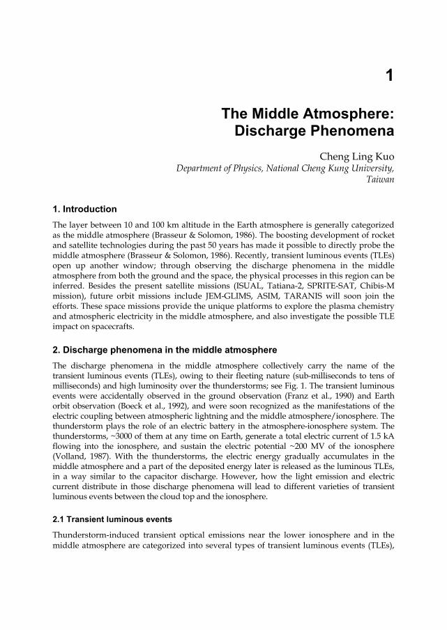
Fig. 1. The known types of transient luminous events (TLEs) between the cloud top and the ionosphere. The causes of TLEs are generally attributed to the activity of cloud discharges. The current known species of TLEs include sprite, elves, blue jet and gigantic jet (Pasko, 2003).

including sprites (Sentman et al., 1995), elves (Fukunishi et al., 1996), blue jets and gigantic jets (Wescott et al., 1995; Pasko et al., 2002; Su et al., 2003).

2.2 Sprites

The University of Minnesota group was the first to obtain the evidence for the existence of the upward electrical discharge on the night of 22, Sep, 1989 (Franz et al., 1990). The first color image of sprites was taken from an aircraft in 1994 that helps to elucidate the luminous structure and its fleeting existence (< 16 ms): a red main body which spans the latitude range between 50 – 90 km, and faint bluish tendrils that extends downward and occasionally reaches the cloud top. The first 0.3 - 1 ms high-speed imaging of sprites, halos and elves were reported by Stanley et al. (1999), Barrington-Leigh et al. (2001) and Moudry et al. (2002, 2003). The high-speed photograph showed that sprites usually initiated at an altitude of ~ 75 km and developed simultaneously upward and downward from the original point (Stanley et al., 1999). In more detail, McHarg et al. (2007) analyzed sub-millisecond (5000 and 7200 frames/s) images of sprites and compiled statistics on velocities of streamer heads. The streamer speeds vary between 106 and 107 m/s. Additionally, Cummer et al. (2006) showed that the long-persisting sprite beads are formed as the tips of the downward moving sprite streamers are attracted to and, sometimes, collide with other streamer channels. Theoretically, higher-speed dynamic evolutions of the fine structure (streamers) in sprites are also predicted by theoretical streamer models (Pasko et al., 1998; Liu & Pasko, 2004; Liu et al., 2006; Liu et al., 2009), which are well consistent with sprite observations.

Among the main groups of emissions in sprites, the molecular nitrogen first positive band (N2 1P) was the first to be identified by using an intensifier CCD spectrograph (Mende et al., 1995). Then, the follow-up works further determined the vibrational exciting states of N2 1P


5

(Green et al., 1996; Hampton et al., 1996) and obtained evidences that support the existence of N2+ Meinel band emission (Bucsela et al., 2003). Recently, 1 ms time-resolution spectrograph observation has been achieved (Stenbaek-Nielse & McHarg, 2004) and the altitude-resolved spectrum (3 ms temporal and ~3 nm spectral resolution between 640 to 820 nm) showed that the population of the upper vibrational state of the N2 1P bands, B3Πg, varies with altitude and is similar to that of the laboratory afterglow at high pressure (Kanmae et al., 2007; Kanmae et al., 2010).

2.3 Elves

The enhanced airglow emission (elves) was first discovered in the images recorded by the space shuttle’s cargo-bay cameras (Boeck et al., 1992; Boeck et al., 1998), and were subsequently observed (and termed as “ELVES” - Emissions of Light and VLF perturbations due to EMP Sources) in the ground observation using a multi-channel high-speed photometer and image intensified CCD cameras (Fukunishi et al., 1996). The Stanford University group built and used an array of photomultipliers called Fly’s Eve to resolve the rapid lateral expansion of optical emissions in elves and the observational results were consistent with those were predicted by the elve model (Inan et al., 1991; Inan et al., 1996; Inan et al., 1997; Barrington-Leigh & Inan, 1999; Barrington-Leigh et al., 2001). The ISUAL experiment on the FORMOSAT-2 satellite, the first spacecraft TLE experiment, then successfully confirmed the existence of ionization and the Lyman-Birge-Hopfield (LBH) band emissions in elves (Mende et al., 2005); the satellite images were used to study their spatial-temporal evolutions and the numerical simulation results of the elve model (Kuo et al., 2007) have beautifully reproduced the observed elve morphology.

2.4 Halos

Halos are pancake-like objects with diameters of ~ 80 km, occurring at altitudes of ~ 80 km (Wescott et al., 2001). Halos were initially thought to be elves by most ground observers using conventional cameras with 30 frames per second until Barrington-Leigh et al. (2001) first proved that halos are distinct from elves (with a much larger diameter of~300 km and a shorter luminous duration of <1ms). The evolution of halo and elves recorded by a high-speed (3000 frames per second) camera were found to be consistent with the modeling results (Barrington-Leigh et al., 2001). Frey et al.(2007) also showed that ~50 % of halos are unexpectedly associated with negative cloud-to-ground (-CG) lightning while nearly 99% sprites are induced by positive cloud-to-ground (-CG) lightning. Wescott et al. (2001) compared the maximum brightness geometry of halos with lightning location using triangulation measurement. They found that the maximum brightness of halo is very close to the location of the parent lightning while the sprite structure can be displaced as far as several tens of kilometers.

2.5 Blue jets and gigantic jets

Blue jets are electric jets that appear to emerge directly from the cloud tops (~ 16-18 km) and shoot upwardly to the final altitudes of ~ 40-50 km (Wescott et al., 1995). Gigantic jets (GJs) are largest discharges in the middle atmosphere, which have been reported by several ground campaigns (Pasko et al., 2002; Su et al., 2003). Based on the monochrome images with a time resolution of 16.7 ms, the temporal optical evolution of the GJs typically contains


6

three stages: the leading jet, the fully-developed jet (FDJ) and the trailing jet (TJ) (Su et al., 2003). The upward propagating leading jet maybe considers being the pre-stage of the FDJ, playing a role similar to that of a stepped leader in the conventional lightning. In the FDJ stage, the GJ optically links the cloud top and the lower ionosphere. The trailing jet shows features similar to those of the blue jets (BJs) and propagates from the cloud top up to ~ 60 km altitude. The optical emission of the trailing jet lasts for more than 0.3 second, and the overall duration of the GJs is ~ 0.5 second (Su et al., 2003).

3. Lightning effect in the middle atmosphere

Since TLEs always occur over active thunderstorms, the electromagnetic radiations from thundercloud discharges being the root cause behind these upper atmospheric luminous phenomena are implied. Thus, to deal with these phenomena, the first two questions should be addressed are "what is the frequency spectrum of a lightning flash and what is the absorption frequency range of the upper atmosphere?" After that one should resolve how the radiation field attenuates in the upper atmosphere and how it reflects at the lower boundary ionosphere.

3.1 Electromagnetic field by lightning current

The lightning frequency spectrum exhibits a peak at 1-10 kHz (Rakov & Uman, 2003, p. 158 and references therein ). If we assume that a lightning has a peak current of 60 kA with a channel resistance of 1 Ω (Rakov & Uman, 2003, p. 398 and references therein ) and radiates all the electromagnetic energy at 5 kHz. The radiated power can be readily computed to be

2 3.6 P I R GW and power flux at 87 km altitude is 0.0378 W/m2. The equivalent energy flux density of the electromagnetic field can be expressed as 2

0c E , where c is the speed of light and 0 is the permittivity of free space. Hence the E strength at 87 km altitude is deduced to be ~3.8 V/m, which is ~ 0.25 times of the conventional breakdown field (Ek) where 1 Ek~117.2 Td and 1 Townsend (Td) = 10-21 V-m2, also refer to the definition of Eq. 1 and Fig. 9). At this altitude, 0.25 Ek corresponds to 14.7 V/m. The reduced E-field is defined as E/N (V-m2) where E is the magnitude of the E-field and N is the neutral density. The reduced E-field for E = 3.8 V/m and N = 1.25×1020 /m3 at an altitude of 87 km is ~ 30.5×10-21 V-m2 or 30.5 Td. The magnitude of E-field (3.8 V/m) is not small comparing to the value of the breakdown E-field (~0.25 Ek), and is sufficient to excite N2 1P (Veronis et al., 1999). As it will be shown, our calculation indicates that a lightning with peak current of 60 kA or higher will generate a sufficiently strong E-field at 87 km elevation to excite the N2 1P emissions of molecular nitrogen. Our results are also consistent with the observational fact that any lightning with peak current > 57 kA will have an accompanying elve (Barrington-Leigh & Inan, 1999).

The wavelength of the lightning radiation field in the VLF frequency range is ~ 10-100 km, which is much longer than the electron mean free path of 1 m at the mesospheric elevation (Rakov & Tuni, 2003). Hence, the lightning electromagnetic field can be approximately thought as a DC field. Those DC electric fields can also be caused by the accumulated charges inside the thundercloud. The quasi-electrostatic field will accelerate ambient electrons. The energized electrons excite the neutral particles (N2 or O2) to higher excited


7

states. The electronically excited neutral particles tend to return to their low energy states, and rapidly de-excite by emitting photons. In next section, we will discuss the atmospheric discharge in the middle atmosphere with an external quasi-electrostatic field.

3.2 Quasi electrostatic field by charge in the thunderstorm

The critical condition of atmospheric discharge occurrence is whether an electron avalanche process in the upper atmosphere does happen in a short time. The time-varying electron number density can be written as

( ) ei a e

dNN

dt (1)

where Ne, i and a are the electron density, the ionization rate and dissociative attachment ( 2

O e O O ) rate, respectively. The values of i and a , which are functions of E-field strength, will be derived from the Boltzmann transport equation and also shown in section 4.5. The criterion of the neutral gas breakdown is decided by Eq. 1 between the electron creation and electron loss term. As i a , the gas breakdown is accompanied by electron avalanche. An avalanche process can begin with a small number of seed electrons, due to existing free electrons or second electrons by cosmic ray, even being triggered by a single electron (Raizer, 1991, pp. 128-130).

The E-field strength at the breakdown threshold ( i a ) is characterized by the breakdown E-field or termed as the conventional breakdown E-field, to distinct it from the positive and the negative streamer breakdown E-fields. The positive and negative streamer breakdown E-fields are the minimum E-fields necessary for the propagation of positive and negative streamer in air at ground pressure. The streamer structures in sprite have been confirmed in TLEs campaign and their radius is roughly several hundreds meter (Gerken & Inan, 2003; Gerken & Inan, 2004). The streamer theory has successfully explained the fine structure of sprite column emissions (Pasko et al., 1998; Liu & Pasko, 2004, 2005; Liu et al., 2006; Liu et al., 2009). The typical values of the conventional breakdown ( kE ), the positive (

crE ) and the negative (

crE ) streamer breakdown E-fields respectively are 532 10kE (Raizer, 1991, p. 135), 512.5 10 (Babaeva & Naidis, 1997), 54.4 10 V/m (Allen & Ghaffar, 1995) in air at ground pressure.

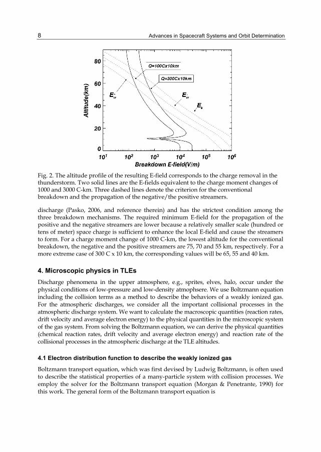
Pasko et al. (1997) has proposed the quasi-electrostatic model to account for the electrostatic interaction between thunderstorm charge and the middle atmosphere. Fig. 2 shows the altitude profile of applied E-field corresponding to the charge remove in the thunderstorm that is defined by charge moment, M Q L where Q is charge in units of coulomb and L is distance above the ground in units of km. The effect of removing total charge Q at altitude z0 = 10 km is equivalent to add the charge in cloud with Gaussian spatial distribution of

2 2 2 20[ / ( ) / ] r a z z be where a = 10km and b = 5 km. Two

solid lines are the applied E-fields equivalent to the charge moment changes of 1000 (100C x 10 km) and 3000 C-km (300C x 10 km). The three dashed lines denote the criterion for the conventional breakdown and the propagation of negative/positive streamers. The conventional breakdown field represent large scale (several hundred km wide) gas


8

Fig. 2. The altitude profile of the resulting E-field corresponds to the charge removal in the thunderstorm. Two solid lines are the E-fields equivalent to the charge moment changes of 1000 and 3000 C-km. Three dashed lines denote the criterion for the conventional breakdown and the propagation of the negative/the positive streamers.

discharge (Pasko, 2006, and reference therein) and has the strictest condition among the three breakdown mechanisms. The required minimum E-field for the propagation of the positive and the negative streamers are lower because a relatively smaller scale (hundred or tens of meter) space charge is sufficient to enhance the local E-field and cause the streamers to form. For a charge moment change of 1000 C-km, the lowest altitude for the conventional breakdown, the negative and the positive streamers are 75, 70 and 55 km, respectively. For a more extreme case of 300 C x 10 km, the corresponding values will be 65, 55 and 40 km.

4. Microscopic physics in TLEs

Discharge phenomena in the upper atmosphere, e.g., sprites, elves, halo, occur under the physical conditions of low-pressure and low-density atmophsere. We use Boltzmann equation including the collision terms as a method to describe the behaviors of a weakly ionized gas. For the atmospheric discharges, we consider all the important collisional processes in the atmospheric discharge system. We want to calculate the macroscopic quantities (reaction rates, drift velocity and average electron energy) to the physical quantities in the microscopic system of the gas system. From solving the Boltzmann equation, we can derive the physical quantities (chemical reaction rates, drift velocity and average electron energy) and reaction rate of the collisional processes in the atmospheric discharge at the TLE altitudes.

4.1 Electron distribution function to describe the weakly ionized gas

Boltzmann transport equation, which was first devised by Ludwig Boltzmann, is often used to describe the statistical properties of a many-particle system with collision processes. We employ the solver for the Boltzmann transport equation (Morgan & Penetrante, 1990) for this work. The general form of the Boltzmann transport equation is


9

{ [ ( , ) ( , )] } ( , , ) ( )

x v collisionq f

v E x t v B x t f x v tt m t

(2)

where ( , , ) f x t is the velocity distribution function, defined such that ( , , ) f x t d is the number density of finding the particle in a unit volume located at position x and at time t with velocity in the range from υ to υ+dυ; q is the charge and m is the mass of electron;

E is

the applied electromagnetic field. The right-hand side, which is the collision term, represents changes in the distribution function due to collision processes.

4.2 Collision process in molecular nitrogen

We consider the following collision processes between electrons and molecular nitrogen:

1. Momentum Transfer: e- + N2 e- + N2 2. Rotational Excitation: e- + N2 e- + N2* 3. Vibrational Excitation: e- + N2 e- + N2* (v=1, 2, 3, 4, 5, 6, 7, and 8) 4. Electronic Excitaion: e- + N2 e- + N2* (A3Σu+, B3Πg, W3Δu, B′ 3Σu-, a′ 1Σu-, a1Πg, w1Δu, C3Πu, E3Σg+, a″1Σg+, Singlet State) 5. Ionization: e- + N2 e- + N2+ + e- (X2Σg+, A2Πu, B2Σu+)

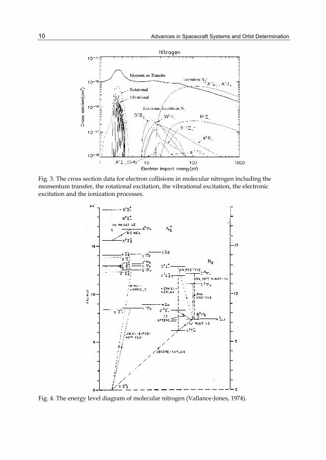
The collision processes between electrons and molecular nitrogen include momentum transfer, rotational excitation, vibrational excitation, electronic excitation and ionization of molecular nitrogen. The total cross section for the electron collision with molecular nitrogen is shown in Fig. 3. The most dominant contribution toward the total cross section is from the

momentum transfer process below 100 eV. The differential cross section

dd

is defined that

the number of electrons which is scattered elastically per second into the solid angle d , 1

e

e e

dNdd N d

. The total cross section can be obtained by integrating

dd

over

the 4 solid angle, m

dd

d (cm2). The momentum transfer cross section for elastic

collisions is defined as (1 cos ) m

dd

d , which is called the effective cross section. For

inelastic collision processes, the cross section could include contributions from the rotational excitation, the vibrational excitation, the electronic excitation and the ionization. The cross sections for inelastic electron collisions in molecular nitrogen are shown in Fig. 3 and the corresponding initiating energies in molecular nitrogen are also shown in Fig. 3, which was compiled by A. V. Phelps.

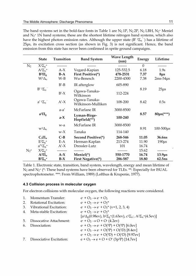
In the energy level diagram of Fig. 4, the electronic excited states are enumerated and labeled by Roman letters, A, B, C, …or a, b, c,… with X indicating the ground state energy level. In the symbol 2 1

/ s

u gX , X is the ground state; S is the spin angular momentum from the unpaired electrons and 2S+1 is the spin multiplicity; Λ is the total angular momentum quantum number. The parities g and u stand for gerade (even in German) or ungerade (odd). For higher total angular momentum Λ, the Greek symbols Σ, Π, Δ and Φ are used.


10

Fig. 3. The cross section data for electron collisions in molecular nitrogen including the momentum transfer, the rotational excitation, the vibrational excitation, the electronic excitation and the ionization processes.

Fig. 4. The energy level diagram of molecular nitrogen (Vallance-Jones, 1974).


11

The band systems set in the bold-face fonts in Table 1 are N2 1P, N2 2P, N2 LBH, N2+ Meniel and N2+ 1N band systems; these are the shortest lifetime nitrogen band systems, which also have the highest photon emission rates. Although the upper state (B′ 3Σu

－) has a lifetime of 25μs, its excitation cross section (as shown in Fig. 3) is not significant. Hence, the band emission from this state has never been confirmed in sprite ground campaigns.

State Transition Band System Wave Length(nm) Energy Lifetime

N2 X1Σg+ -------- ------- ------- 0 ------- A3Σu+ A-X Vegard-Kapian 125-532.5 6.18 1.9s B3Πg B-A First Positive(*) 478-2531 7.37 8μs W3Δu W-B Wu-Benesch 2200-4300 7.38 2ms-54μs

B′ 3Σu

－ B′-B IR afterglow 605-890

8.19 25μs B′-X Ogawa-Tanaka-

Wilkinson 112-224

a′ 1Σu－ A′-X Ogawa-Tanaka-

Wilkinson-Mulliken 108-200 8.42 0.5s

a1Πg

a-a′ McFarlane IR 3000-8500 8.57 80μs(***)

a-X Lyman-Birge-Hopfield(**) 100-240

w1Δu

w-a McFarlane IR 3000-8500 8.91 100-500μs

w-X Tanaka 114-140 C3Πu C-B Second Positive(*) 268-546 11.05 36.6ns E3Σg+ E-A Herman-Kaplan 213-274 11.90 190μs a″1Σg+ A′-X Dressler-Lutz 101 16.74

N2+ X2Σg+ -------- -------- -------- 15.62 -------- A2Πu A-X Meniel(*) 550-1770 16.74 13.9μs B2Σu+ B-X First Negative(*) 286-587 18.80 62.5ns

Table 1. Electronic state, transition, band system, wavelength, energy and mean lifetime of N2 and N2+ (*: These band systems have been observed for TLEs. **: Especially for ISUAL spectrophotometer. ***: From William, 1989) (Lofthus & Krupenie, 1977).

4.3 Collision process in molecular oxygen

For electron collisions with molecular oxygen, the following reactions were considered.

1. Momentum Transfer: e- + O2 e- + O2 2. Rotational Excitation: e- + O2 e- + O2* 3. Vibrational Excitation: e- + O2 e- + O2* (v=1, 2, 3, 4) 4. Meta-stable Excitation: e- + O2 e- + O2* [a1Δg(0.98ev), b1Σg+(1.63ev), c1Σu-, A3Σu+(4.5ev)] 5. Dissocative Attachment: e- + O2 O + O- (4.2ev) 6. Dissociation: e- + O2 e- + O(3P) + O(3P) [6.0ev] e- + O2 e- + O(3P) + O(1D) [8.4ev] e- + O2 e- + O(3D) + O(1D) [9.97ev] 7. Dissociative Excitation: e + O2 e + O + O* (3p3P) [14.7ev]


12

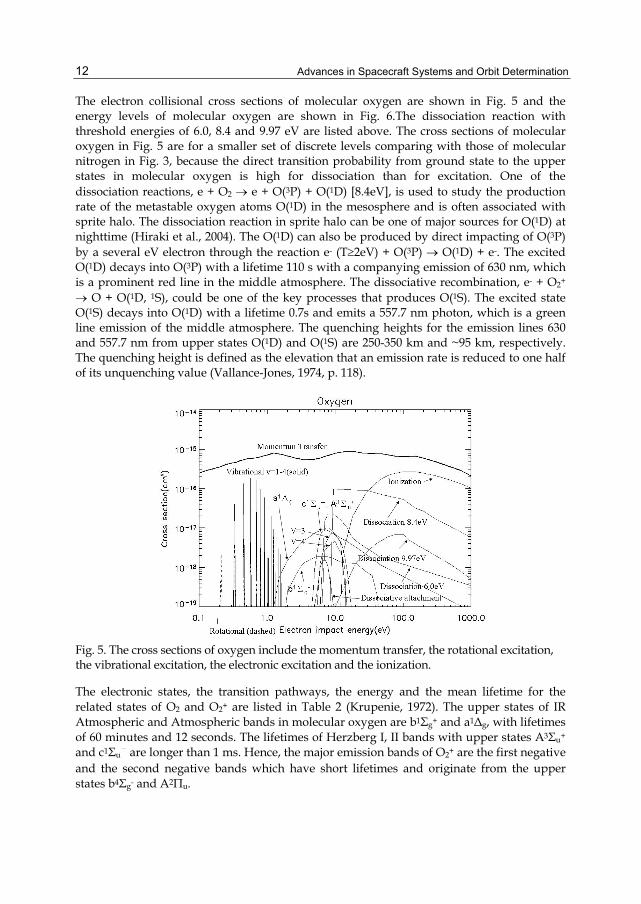
The electron collisional cross sections of molecular oxygen are shown in Fig. 5 and the energy levels of molecular oxygen are shown in Fig. 6.The dissociation reaction with threshold energies of 6.0, 8.4 and 9.97 eV are listed above. The cross sections of molecular oxygen in Fig. 5 are for a smaller set of discrete levels comparing with those of molecular nitrogen in Fig. 3, because the direct transition probability from ground state to the upper states in molecular oxygen is high for dissociation than for excitation. One of the dissociation reactions, e + O2 e + O(3P) + O(1D) [8.4eV], is used to study the production rate of the metastable oxygen atoms O(1D) in the mesosphere and is often associated with sprite halo. The dissociation reaction in sprite halo can be one of major sources for O(1D) at nighttime (Hiraki et al., 2004). The O(1D) can also be produced by direct impacting of O(3P) by a several eV electron through the reaction e- (T2eV) + O(3P) O(1D) + e-. The excited O(1D) decays into O(3P) with a lifetime 110 s with a companying emission of 630 nm, which is a prominent red line in the middle atmosphere. The dissociative recombination, e- + O2+ O + O(1D, 1S), could be one of the key processes that produces O(1S). The excited state O(1S) decays into O(1D) with a lifetime 0.7s and emits a 557.7 nm photon, which is a green line emission of the middle atmosphere. The quenching heights for the emission lines 630 and 557.7 nm from upper states O(1D) and O(1S) are 250-350 km and ~95 km, respectively. The quenching height is defined as the elevation that an emission rate is reduced to one half of its unquenching value (Vallance-Jones, 1974, p. 118).

Fig. 5. The cross sections of oxygen include the momentum transfer, the rotational excitation, the vibrational excitation, the electronic excitation and the ionization.

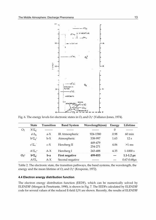
The electronic states, the transition pathways, the energy and the mean lifetime for the related states of O2 and O2+ are listed in Table 2 (Krupenie, 1972). The upper states of IR Atmospheric and Atmospheric bands in molecular oxygen are b1Σg+ and a1Δg, with lifetimes of 60 minutes and 12 seconds. The lifetimes of Herzberg I, II bands with upper states A3Σu+ and c1Σu

－ are longer than 1 ms. Hence, the major emission bands of O2+ are the first negative and the second negative bands which have short lifetimes and originate from the upper states b4Σg- and A2Πu.


13

Fig. 6. The energy levels for electronic states in O2 and O2+ (Vallance-Jones, 1974).

State Transition Band System Wavelength(nm) Energy Lifetime

O2 X3Σg- -------- ------- ------- 0 ------- a1Δg a-X IR Atmospheric 924-1580 0.98 60 min b1Σg+ b-X Atmospheric 538-997 1.63 12 s

c1Σu－ c-X Herzberg II

449-479 254-271

4.06 >1 ms

A3Σu+ A-X Herzberg I 243-488 4.35 1-1000 s

O2+ b4Σg- b-a First negative 499-853 --- 1.1-1.2 μs A2Πu A-X Second negative ------- --- 0.67-0.68μs

Table 2. The electronic state, the transition pathways, the band systems, the wavelength, the energy and the mean lifetime of O2 and O2+ (Krupenie, 1972).

4.4 Electron energy distribution function

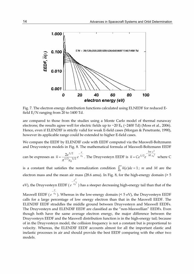
The electron energy distribution function (EEDF), which can be numerically solved by ELENDIF (Morgan & Penetrante, 1990), is shown in Fig. 7. The EEDFs calculated by ELENDIF code for several values of the reduced E-field E/N are shown. Recently, the results of ELENDIF


14

Fig. 7. The electron energy distribution functions calculated using ELNEDF for reduced E-field E/N ranging from 20 to 1400 Td.

are compared to those from the studies using a Monte Carlo model of thermal runaway electrons; the results agree well for electric fields up to ~20 Ek (~2400 Td) (Moss et al., 2006). Hence, even if ELENDIF is strictly valid for weak E-field cases (Morgan & Penetrante, 1990), however its applicable range could be extended to higher E-field cases.

We compare the EEDF by ELENDIF code with EEDF computed via the Maxwell-Boltzmann and Druyvesteyn models in Fig. 8. The mathematical formula of Maxwell-Boltzmann EEDF

can be expresses as 0

1/2

1/2 3/20

2 n e

. The Druyvesteyn EEDF is

2

20

3

1/2

m

Mn C e

where C

is a constant that satisfies the normalization condition 0

( ) 1

n d ; m and M are the

electron mass and the mean air mass (28.6 amu). In Fig. 8, for the high-energy domain (> 5

eV), the Druyvesteyn EEDF (

2

20

e

) has a steeper decreasing high-energy tail than that of the

Maxwell EEDF ( 0

e ). Whereas in the low-energy domain (< 5 eV), the Druyvesteyn EEDF

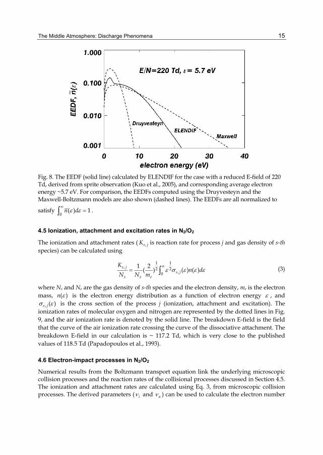
calls for a large percentage of low energy electron than that in the Maxwell EEDF. The ELENDIF EEDF straddles the middle ground between Druyvesteyn and Maxwell EEDFs. The Druyvesteyn and ELENDIF EEDF are classified as the “non-Maxwellian” EEDFs. Even though both have the same average electron energy, the major difference between the Druyvesteyn EEDF and the Maxwell distribution function is in the high-energy tail; because of in the Druyvesteyn model, the collision frequency is not a constant but is proportional to velocity. Whereas, the ELENDIF EEDF accounts almost for all the important elastic and inelastic processes in air and should provide the best EEDF comparing with the other two models.


15

Fig. 8. The EEDF (solid line) calculated by ELENDIF for the case with a reduced E-field of 220 Td, derived from sprite observation (Kuo et al., 2005), and corresponding average electron energy ~5.7 eV. For comparison, the EEDFs computed using the Druyvesteyn and the Maxwell-Boltzmann models are also shown (dashed lines). The EEDFs are all normalized to

satisfy 0

( ) 1

n d .

4.5 Ionization, attachment and excitation rates in N2/O2

The ionization and attachment rates ( ,s jK is reaction rate for process j and gas density of s-th species) can be calculated using

1 1

, 2 2,0

1 2( ) ( ) ( )

s js j

s e e

Kn d

N N m (3)

where Ns and Ne are the gas density of s-th species and the electron density, me is the electron mass, ( )n is the electron energy distribution as a function of electron energy , and

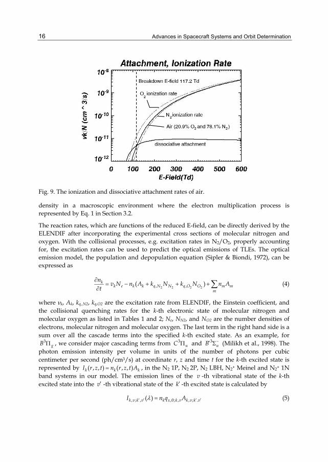
, ( )s j is the cross section of the process j (ionization, attachment and excitation). The ionization rates of molecular oxygen and nitrogen are represented by the dotted lines in Fig. 9, and the air ionization rate is denoted by the solid line. The breakdown E-field is the field that the curve of the air ionization rate crossing the curve of the dissociative attachment. The breakdown E-field in our calculation is ~ 117.2 Td, which is very close to the published values of 118.5 Td (Papadopoulos et al., 1993).

4.6 Electron-impact processes in N2/O2

Numerical results from the Boltzmann transport equation link the underlying microscopic collision processes and the reaction rates of the collisional processes discussed in Section 4.5. The ionization and attachment rates are calculated using Eq. 3, from microscopic collision processes. The derived parameters ( i and a ) can be used to calculate the electron number


16

Fig. 9. The ionization and dissociative attachment rates of air.

density in a macroscopic environment where the electron multiplication process is represented by Eq. 1 in Section 3.2.

The reaction rates, which are functions of the reduced E-field, can be directly derived by the ELENDIF after incorporating the experimental cross sections of molecular nitrogen and oxygen. With the collisional processes, e.g. excitation rates in N2/O2, properly accounting for, the excitation rates can be used to predict the optical emissions of TLEs. The optical emission model, the population and depopulation equation (Sipler & Biondi, 1972), can be expressed as

2 2 2 2, ,( )

kk e k k q N N q O O m m

m

nv N n A k N k N n A

t (4)

where νk, Ak, kq,,N2, kq,O2 are the excitation rate from ELENDIF, the Einstein coefficient, and the collisional quenching rates for the k-th electronic state of molecular nitrogen and molecular oxygen as listed in Tables 1 and 2; Ne, NN2, and NO2 are the number densities of electrons, molecular nitrogen and molecular oxygen. The last term in the right hand side is a sum over all the cascade terms into the specified k-th excited state. As an example, for

3gB , we consider major cascading terms from 3uC and 3 uB (Milikh et al., 1998). The photon emission intensity per volume in units of the number of photons per cubic centimeter per second (ph/cm3/s) at coordinate r, z and time t for the k-th excited state is represented by ( , , ) ( , , )k k kI r z t n r z t A , in the N2 1P, N2 2P, N2 LBH, N2+ Meinel and N2+ 1N band systems in our model. The emission lines of the v -th vibrational state of the k-th excited state into the v -th vibrational state of the k -th excited state is calculated by

, ; , ,0; , , ; .( ) k v k v k x k v k v k vI n q A (5)


17

where nk is the number density of the ambient molecular nitrogen or molecular oxygen; qx,0;k,v is the Franck-Condon factor, which represents the relative population of the v-th vibrational level of the k-th excited state from the 0-th vibrational state of the ground state; Ak,v;k’,v’ is the Einstein coefficient from the v-th vibrational state of k-th electronic state to the v -th vibrational state of k -th electronic state, and the adopted values for molecular

nitrogen is from (Gilmore et al., 1992) and those values for molecular oxygen from (Krupenie, 1972).

4.7 Full kinetic scheme in discharge gas

Besides electron-impact processes between electron and N2/O2, other plasma chemistry reactions also needed to be considered for the discharge processes in TLEs. Recently, Sentman et al. (2008) proposed the full-kinetic plasma chemistry model to compute the involved plasma processes in TLEs; in all, +80 species and +500 chemical reactions are considered in their zero dimensional plasma chemistry model. Sentman et al. (2008) pointed out that the optical emissions in the tail of the sprite streamer may be due to chemiluminescent processes, which follow the electron-impact processes in the head of the sprite streamer. Kuo et al. (Kuo et al., 2011) adopted the Sentman kinetic scheme but include a few corrected chemical processes for a similar but independent plasma chemistry study of TLEs. Kuo et al. (Kuo et al., 2011) found that the modelling intensity ratios N2 1P/N2 2P, N2+ 1N/N2 2P were in good agreement with ISUAL optical measurements. Moreover, they also reported, for the first time, the evidence for the existence of O2 atmosphere (0-0) band in sprites that was predicted by the plasma chemistry model (Sentman et al., 2008; Sentman & Stenbaek-Nielsen, 2009).

5. Space shuttle observations of TLEs

Recently, a few review articles on the TLE orbit missions and their results have been available (Yair, 2006; Lefeuvre et al., 2009; Neubert, 2009; Panasyuk et al., 2009; Pasko, 2010; Pasko et al., 2011). Here, only the relevant orbit missions are revisited and summarized. Before the first satellite mission (ISUAL) for the TLE survey, pioneer quests for the TLE observations had been performed on the space shuttles and on the International Space Station (ISS). The first TLE observed from space was termed as an enhanced airglow emission (Boeck et al., 1992); an elve in the current term. They performed post-reviews of the video tapes recorded by the cargo-bay television cameras from the STS-41 mission of the shuttle Discovery, and identified the enhanced transient luminosity events in the airglow altitude of ~ 95 km. Boeck et al. (Boeck et al., 1992) concluded that the enhanced airglow emission suddenly appeared after a lightning flash, and provided the evidence on the direct coupling between atmospheric lighting and enhanced airglow emission in the bottom of ionosphere (Boeck et al., 1992; Boeck et al., 1995; Boeck et al., 1998).

The Mediterranean Israeli Dust Experiment (MEIDEX) sprite campaign was conducted on board the space shuttle Columbia (Yair et al., 2003; Yair et al., 2004; Yair, 2006) during the STS-107 mission in January 2003. Using an image-intensified Xybin IMC-201 camera, 17 TLEs were identified ( 7 sprites and 10 elves) along with additional 20 probable events. Their brightness in the 665 nm filter is determined to be in the range of 0.3-1.7 MR and 1.44-1.7 MR in the 860-nm filter (Israelevich et al., 2004; Yair et al., 2004).


18

The LSO (Lightning and Sprite Observations) on board ISS (International Space Station) is first experiment dedicated to a nadir observation of sprites from the Earth orbit (Blanc et al., 2004; Blanc et al., 2006; Blanc et al., 2007). The first LSO measurements were conducted on the ISS in October 2001. Blanc et al. (Blanc et al., 2004) utilized the emission differentiation method designed for the nadir observation of TLEs to distinguish the sprite emissions from the lighting emissions. The LSO is a pilot experiment for the upcoming TARANIS satellite mission. The configuration of the nadir observation is necessary for a simultaneous study of the optical, the relativistic runaway electron, and the X-gamma emissions from the TLEs.

5.1 The first satellite mission for the survey of TLEs: ISUAL

ISUAL (Imager of Sprites and Upper Atmospheric Lightnings) onboard the FORMOSAT-2 satellite is first satellite payload dedicating for the survey of TLEs (Chern et al., 2003; Mende et al., 2005; Su et al., 2005; Hsu et al., 2009). The FORMOSAT-2 is a sun-synchronized satellite with fourteen daily-revisiting 891 km altitude orbits. The FORMOSAT-2 was successfully launched on 21 May 2004. The ISUAL experiment is an international collaboration between the National Cheng Kung University, Taiwan, Tohoku University, Japan and the instrument development team from the University of California, Berkeley. The ISUAL consists of three sensor packages including an intensified CCD imager, a six-channel spectrophotometer and a dual-band array photometer. The imager is equipped with 6 selectable filters (N2 1P, 762, 630, 557.7, 427.8 nm filters, and a broadband filter) mounted on a rotatable filter wheel. The spectrophotometer contains six filter photometer channels, their bandpasses ranging from the far ultraviolet to the near infrared regions. The dual-channel AP is fitted with broadband blue and red filters. The mission objectives are to perform a global survey of lightning-induced TLEs, to determine the occurrence rate of TLEs above thunderstorm, to investigate their spatial, temporal and spectral properties, and to investigate of the global distribution of airglow intensity as a function of altitude. ISUAL have completed the first phase (2004-2009) of the orbital mission. Due to a successful five-year mission and the significant scientific achievements, an additional funding has been granted to the ISUAL team for an extended mission of +3 years (2010-2014) from the National Space Organization in Taiwan.

The first sprite from ISUAL was recorded on July 4, 2004/21:31:15.451. From analyzing the ISUAL spectrophotometer data, Kuo et al. (2005) and Liu et al. (2006) estimated the strength of electric field at the streamer tips to be 2-4 Ek; through analyzing the ISUAL array photometer data, Adachi et al. (2006) concluded that the electric field is 1-2 Ek in the diffuse region of the sprite streamer. Recently, based on sprite streamer simulations, (Celestin & Pasko, 2010) pointed out that the electric fields derived basing on the ISUAL spectrophotometer/photometer data were lower-limiting values, since the time of the highest electric field precedes that of detected emission peak for the N2 excited emission bands. The highest band emission source spatially is behind the electric field peak in streamer simulations, and they estimated that reported electric field strengths should be corrected by multiplying a factor of ~1.5 (Celestin & Pasko, 2010).

Mende et al. (2005) analyzed ISUAL elves whose parent lightning were behind the Earth limb and hence the lightning emissions were blocked by the solid Earth; they reported that the elves contained significant 391.4 nm emission of 1NN2+. Mende et al. (2005) also estimated that reduced electric field in elves was > 200 Td by comparing the ratio of elve-


19

emissions registered by different channels of the ISUAL spectrophotometer and that of the theoretically-derived emission intensity ratio. Using the inferred reduced electric field and the total ionization derived from the registered 1NN2+ emission, they also found that, on average, the free electron density is 210 electrons cm-3 in elves; in the region occupied by an elve, the free electron density increases by nearly 100% over the ambient E-layer ionospheric value. Moreover, the FUV emission (Lyman-Birge-Hopfield band) in TLEs was also detected for the first time (Mende et al., 2005). Kuo et al. (2007) developed an elve model using finite difference time domain method to simulate the expected geometry of ISUAL recorded elves and the expected photometric intensities of elves. Their simulation results were in excellent agreement with ISUAL observed events. Kuo et al. (2007) also found there is an exponential relationship between the causative lighting current and the elve emissions. Based on their results, the peak current of the elve-parent lightning can be inferred from the ISUAL photometric intensity data.

Using the ISUAL TLE data, Chen et al. (2008) constructed the first global TLE distribution map and obtained the global TLE occurrence rates. The map indicates that there are six elve hot zones over: the Caribbean Sea, the South China Sea, the east Indian Ocean, the central Pacific Ocean, the west Atlantic Ocean, and the southwest Pacific Ocean. Unlike sprites mostly occur over the lands; elves appear predominately over oceans. Chen et al. (2008) compiled the global occurrence rate of elves and concluded that elve occurrence rate jumps as the sea surface temperature exceeds 26 degrees Celsius. Their finding clearly confirms the existence of an ocean-atmosphere-ionosphere coupling. Kuo et al. (2008) analyzed the photometric and the imagery brightness of TLEs (sprites, halos and elves), and found that total energy deposition rate of TLEs is ~1 GJ/min in the middle atmosphere. Hsu et al. (2009) re-examed a more complete set of ISUAL recorded TLEs, and discovered that the global TLE occurrence rates should be 72, 3.7, and ~1 events/minute, respectively, for elvess, halos, and sprites. Comparing with the results from the first three years of the ISUAL experiment reported in Chen et al. (2008), the global occurrence rates for elves and halos are higher due to the adoption of different correction factors. Using these updated TLE rates, the free electron content over an elve hot zone is estimated to be elevated by more than 10%. Deposited energy in the upper atmosphere by sprites, halos, and elves was found to be 22, 14, and 19 MJ per event, respectively. After factoring in the occurrence rates, in each minute, sprites, halos and elves deliver 22, 52 and 1370 MJs of the troposphere energy to the upper atmosphere.

Using ISUAL recorded gigantic jets, Kuo et al. (2009) performed the first high time resolution analysis of these spectacular events. They reported that the velocity of the upward propagating fully-developed jet of the gigan �tic jets was ~107 m/s, which is in line with that for the downward sprite streamers. Analysis of the spectral ratios of the fully-developed jet emissions gives a reduced E field of > 5 Ek and average electron energy of 8.5–12.3 eV in the gigantic jets. These values are higher than those in the sprites but are similar to those predicted by streamer models (Kuo et al., 2005), which implies the existence of streamer tips in fully-developed jets.

Chou et al. (2010) found that the gigantic jets (GJs) can actually be categorized into three types from their generating sequence and spectral properties. Type I GJs resembles that reported previously in (Su et al., 2003): after the fully-developed jet (FDJ) established the discharge channel, the ISUAL photometers registered a peak that was from a return stroke-


20

like-process between the ionosphere and the cloud-top. The associated ULF (ultra low frequency) sferics indicates that they are negative cloud-to-ionosphere discharges (-CIs). Type II GJs begin as blue jets and then developed into GJs in ~100 ms. Blue jets also frequently occurred at the same region before and after the type II GJs. No identifiable ULF sferics of the type II Gjs were found, though an extra event with +CI ULF is probably a type II GJ. Thus for the type II GJs, the energy and the charge may not accumulate high enough to initiate a bright gigantic jet. Type III GJs were preceded by lightning and a GJ occurred near this preceding lightning. The spectral data of the type III GJs are dominated by lightning signals and the ULF data have high background noise. The average brightness of the type III GJs falls between those of the other two types of GJs. Therefore, they proposed that the discharge polarity of the type III GJs can be either negative or positive, depending on the type of the charge imbalance left by the trigger lightning (Chou et al., 2010).

After analyzing the N2 1P brightness of the ISUAL elves and their FUV intensity and performing modeling work of elves, Chang et al. (2010) shown that ISUAL-FUV intensity in an elve could be used to infer the peak current of the causative CG lightning. The ISUAL detection rate of elves is also can be improved since the sensitivity of ISUAL FUV photometer is 16 times higher than that of ISUAL N2 1P-filtered Imager. Hence, FUV photometer can be used to perform a global elve survey and to obtain the peak current of the elve-producing lighting and other salient parameters. Besides, the existences of multi-elves, which are FUV events from the M-components or the multiple strokes in lighting flashes, were also reported.

Lee et al. (2010) analyzed the distribution of the TLEs registered by ISUAL, and deduced the synoptic-scale factors that control the occurrence of TLEs. Two different distribution patterns are found. For the low‐latitude tropical regions (25°S ~ 25°N), 84% of the TLEs were found to occur over the Intertropical Convergence Zone (ITCZ) and the South Pacific Convergence Zone. The distribution of TLEs exhibited a seasonal variation that migrates north and south with respect to the equator. For the mid-latitude regions (latitudes beyond ±30°), 88% of the northern winter TLEs and 72% of the southern winter TLEs occurred near the mid-latitude cyclones. The winter TLE occurrence density and the storm‐track frequency share similar trends with the distribution of the winter TLEs offset by 10°–15°.

5.2 Other present orbital missions of TLEs

Besides ISUAL mission (2004-) (Chern et al., 2003; Mende et al., 2005; Su et al., 2005; Hsu et al., 2009) for the global survey of TLEs, Tatiana-1 (2005-7) mission performed a similar function; Tatiana is a Moscow State University research educational microsatellite Tatiana. Tatiana mission was carried out in the period between January 2005 and March 2007 (Garipov et al., 2005; Garipov et al., 2006; Shneider & Milikh, 2010). With the Tatiana-1 data, Shneider and Milikh (2010) studied the atmospheric electricity phenomena that can serve as sources for short millisecond range flashes; they reported that the UV flashes in the millisecond scale detected by Tatiana-1 may have been generated by gigantic blue jets (GBJ).

Tatiana-2 (2009-) satellite was launched on 17 September 2009 to a solar-synchronized orbit of 820 km altitude with a inclination angle 98.8°(Garipov et al., 2010). The Tatiana-2 satellite have upgraded their instrument to achieve an higher performance than Tatiana-1 mission in several ways: UV (300-400 nm)- and red (600-700 nm)-filtered photomultiplier tube (PMT)


21

micro-electro-mechanical telescope for extreme lighting (MTEL), photo spectrometer and electron flux detector (Panasyuk et al., 2009; Garipov et al., 2010).

SPRITE-SAT (2010-) is a Japanese micro satellite with a size of 50 cm cube and with a weight of 45 kg, that were designed and developed by Tohoku University, Japan (Takahashi et al., 2010). SPRITE-SAT has a sun-synchronous polar orbit of 670 km altitude. The main scientific goal of SPRITE-SAT satellite is to simultaneously observe TLEs and terrestrial gamma-ray flashes in nadir direction and to study the relationship and generation mechanisms of TLEs and TGFs. SPRITE-SAT has equipped the lightning Imager-1 and Imager-2 with narrow- and wide-band 762 nm filters; the payload include a wide field-of-view camera with a FOV of 140°, a terrestrial gamma-ray counter with a FOV of 134x180°, a high-sensitivity star sensor, and a VLF receiver and antenna. The SPRITE-SAT has been successful launched on 23 January 2009 and is currently operating by the Tohoku University group.

Chibis-M mission (Klimov et al., 2009) (see http://chibis.cosmos.ru/) is another ISS module with the goal to study TLEs and TGFs. Scientific instruments of Chibis-M include X-ray and γ-ray detectors with an energy range of 50-500 eV & a time resolution of 30 ns, an UV detector sensitive in the wavelength band of 180-800 nm, a digital photo camera with a fixed exposure time if 0.2 second, a radiofrequency sensor with a frequency passing band of 20 – 50 Hz, and an ULF-VLF antenna. On January 25, 2012 the micro-satellite Chibis (lapwing) was successfully detached from the transportation vehicle <Progress M-13> and started its mission. Video of the "Chibis-M" detachment from "Progress" can be seen on http://www.roscosmos.ru/main.php?id=216. This mission is dedicated to studies of Terrestrial Gamma-ray Flashes (TGFs) and accompanying emissions above thunderstorms in the upper atmosphere. The multi-instrument technique, covering nearly the whole spectrum of electromagnetic emissions (radio, optical, UV, X-ray and gamma bands), will monitor the lightning discharges with higher time resolution.

5.3 Future orbital missions of TLEs

Global Lightning and sprIte MeasurementS on JEM-EF (JEM-GLIMS, 2011-) is a space mission to observe lightning and TLEs from the Exposure Facility (EF) of the Japanese Experiment Module (JEM) on the International Space Station (ISS). The JEM-GLIMS mission uses two CMOS cameras, two photometers, one spectro-imager, and two VHF receivers to achieve the mission goals of studying the generation mechanism of transient luminous events (TLEs) and identifying the relationship between lightning, TLEs, and terrestrial γ-ray flashes (TGFs) (Sato et al., 2009).

ASIM (Atmpshere-Space Interactions Monitor, 2014-) (Neubert, 2009) is an instrument suite, mounted on the external platform of the European Columbus module for the International Space Station (ISS). The scientific objectives are to understand the global occurrences of TLEs and TGFs, to study the physical mechanism of TLEs and TGFs, and their relationships. The ASIM will further coordinates with the ground EuroSprite campaigns (Neubert et al., 2001; Neubert et al., 2008; Neubert, 2009).

TARANIS (Tool for the Analysis of Radiations from lightNIngs and Sprites, 2016-) (Blanc et al., 2006; Lefeuvre et al., 2009) is a CNES satellite project with a goal to study of the impulsive transfer of energy between the Earth atmosphere and the space environment. TARANIS have a very broad range of scientific objectives for simultaneously probing the


22

TLEs and Terrestrial Gamma-ray Flashes (TGFs). Therefore, TARANIS instruments including micro-cameras, photometers, X-ray, γ-ray detectors, energetic electron detectors, and radio band antenna. The TRANIS mission aims are: (1) to advance the physical understanding of the links between TLEs, TGFs, (2) to clarify the potential signatures of impulsive transfers of energy, verified by physical mechanism, and (3) to elucidate the physical parameters in TLEs and TGFs (Blanc et al., 2006; Lefeuvre et al., 2009).

6. The impact of TLEs on space shuttle

Space shuttle uses 76 miles (122 km) as their re-entry altitude, which roughly marks the boundary where atmospheric drag becomes important. Below re-entry altitude, space shuttle switches from steering with thrusters to maneuvering with air surfaces. At lower altitude, space shuttle enters the TLE region (10 – 100 km). The magnitude of electric field can as high as 2-3 Ek (10 – 40 V/m) in elves altitudes of 80 - 100 km (Kuo et al., 2007). The average energy of accelerated electrons in elves can as high as several to tens of eV (Kuo et al., 2005; Kuo et al., 2007). In the high tail of electron energy distribution, runaway electron may be up to several kilo electron volt of electron energy. Besides, these energetic electron avalanches in gas breakdown may cause the plasma erosion on the heat shield of space shuttle. Therefore, it is necessary to have space missions to investigate the possible damages on re-entry of space shuttle.

7. Conclusion

Discharge phenomena in the middle atmosphere are one of the hottest research fields for satellite missions; currently with the ISUAL, the Tatiana-2, the SPRITE-SAT, Chibis-M missions perform daily observations of TLEs from space. Other upcoming orbit missions including JEM-GLIMS, ASIM, TARANIS will soon join in to carry out further investigations of these interesting phenomena. These space missions will continue hunting TLEs over the thunderstorm and exploring the associated plasma physics, plasma chemistry, and atmospheric electricity in middle atmosphere. Besides, high electric field pulses and energized electron-impact process may cause the damage as space shuttle flies back to the TLE altitudes (10-100 km).

8. Acknowledgments

We thank Profs. Rue-Ron Hsu and Han-Tzong Su at the National Cheng Kung University, Prof. Lou-Chuug Lee at the National Central University, Prof. Alfred Chen at the National Cheng Kung University, Prof. J. L. Chern at the National Chiao Tung University, Drs. Harald Frey and Stephen Mende at the Space Science Laboratory-University of California, Profs. Horoshi Fukunishi and Yukihiro Takahashi at Tohoku University for helpful discussions and comments. We are also grateful to the National Center for High-performance Computing in Taiwan and Center for Computational Geophysics at National Central University for computer time and facilities. This work was supported in part by grants (NSC 98-2111-M-008-001, NSC 99-2111-M-006-001-MY3, NSC 99-2112-M-006-006-MY3, NSC 099-2811-M-006-004, NSC 100-2119-M-006-015, NSC 100-2811-M-006-004) from National Science Council in Taiwan.


23

9. References

Adachi, T., et al. (2006). Electric field transition between the diffuse and streamer regions of sprites estimated from ISUAL/array photometer measurements. Geophys. Res. Lett., Vol.33, (September 1, 2006), pp. 17803, DOI: 10.1029/2006GL026495.

Allen, N. L., & Ghaffar, A. (1995). The conditions required for the propagation of a cathode-directed positive streamer in air. J. Phys. D., Vol.28, (February 1, 1995), pp. 331-337, DOI: 10.1088/0022-3727/28/2/016.

Babaeva, N. Y., & Naidis, G. V. (1997). Dynamics of positive and negative streamers in air in weak uniform electric fields. IEEE Trans. Plasma Sci., Vol.25, No.2, pp. 375-379, DOI: 10.1109/27.602514.

Barrington-Leigh, C. P., & Inan, U. S. (1999). Elves triggered by positive and negative lightning discharges. Geophys. Res. Lett., Vol.26, (March 1, 1999), pp. 683-686, DOI: 10.1029/1999GL900059.

Barrington-Leigh, C. P.; Inan, U. S., & Stanley, M. (2001). Identification of sprites and elves with intensified video and broadband array photometry. J. Geophys. Res., Vol.106, (February 1, 2001), pp. 1741-1750, DOI: 10.1029/2000JA000073.

Blanc, E., et al. (2004). Nadir observations of sprites from the International Space Station. J. Geophys. Res., Vol.109, No.A2, pp. A02306, 0148-0227, DOI: 10.1029/2003ja009972.

Blanc, E., et al. (2006).Observations of sprites from space at the nadir: the lso (lightning and sprite observations) experiment on board of the international space station In: Sprites, Elves and Intense Lightning Discharges, pp.151-166, Springer Netherlands, ISBN 978-1-4020-4629-2.

Blanc, E., et al. (2007). Main results of LSO (Lightning and sprite observations) on board of the international space station. Microgravity Science and Technology, Vol.19, No.5, pp. 80-84, 0938-0108, DOI: 10.1007/bf02919458.

Boeck, W. L., et al. (1992). Lightning induced brightening in the airglow layer. Geophys. Res. Lett., Vol.19, (January 1, 1992), pp. 99-102, DOI:10.1029/91GL03168.

Boeck, W. L., et al. (1995). Observations of lightning in the stratosphere. J. Geophys. Res., Vol.100, (January 1, 1995), pp. 1465-1476, DOI: 10.1029/94JD02432.

Boeck, W. L., et al. (1998). The role of the space shuttle videotapes in the discovery of sprites, jets and elves. J. Atmos. Sol. Terr. Phys., Vol.60, (May 1, 1998), pp. 669-677, DOI: 10.1016/S1364-6826(98)00025-X.

Brasseur, G., & Solomon, S. (1986). Aeronomy of the middle atmosphere : chemistry and physics of the stratosphere and mesosphere (2nd), D. Reidel Pub. Co., ISBN 902-7723-44-3, Dordrecht.

Bucsela, E., et al. (2003). N2(B3g) and N2+(A2u) vibrational distributions observed in sprites. J. Atmos. Sol. Terr. Phys., Vol.65, (March 2003), pp. 583-590, ISSN 1364-6826, DOI: 10.1029/96GL02071.

Celestin, S., & Pasko, V. P. (2010). Effects of spatial non-uniformity of streamer discharges on spectroscopic diagnostics of peak electric fields in transient luminous events. Geophys. Res. Lett., Vol.37, No.7, pp. L07804, 0094-8276, DOI: 10.1029/2010gl042675.

Chang, S. C., et al. (2010). ISUAL far-ultraviolet events, elves, and lightning current. J. Geophys. Res., Vol.115, pp. A00E46, 0148-0227, DOI: 10.1029/2009ja014861.

Chen, B., et al. (2008). Global distributions and occurrence rates of transient luminous events. J. Geophys. Res., Vol.113, pp. A08306, DOI:10.1029/2008JA013101.


24

Chern, J. L., et al. (2003). Global survey of upper atmospheric transient luminous events on the ROCSAT-2 satellite. J. Atmos. Sol. Terr. Phys., Vol.65, (March 1, 2003), pp. 647-659, DOI: 10.1016/S1364-6826(02)00317-6.

Chou, J. K., et al. (2010). Gigantic jets with negative and positive polarity streamers. J. Geophys. Res., Vol.115, pp. A00E45, 0148-0227, DOI: 10.1029/2009ja014831.

Cummer, S. A., et al. (2006). Submillisecond imaging of sprite development and structure. Geophys. Res. Lett., Vol.33, (February 1, 2006), pp. 04104, DOI: 10.1029/2005GL024969.

Franz, R. C.; Nemzek, R. J., & Winckler, J. R. (1990). Television Image of a Large Upward Electrical Discharge Above a Thunderstorm System. Science, Vol.249, (July 1, 1990), pp. 48-51, DOI: 10.1126/science.249.4964.48.

Frey, H. U., et al. (2007). Halos generated by negative cloud-to-ground lightning. Geophys. Res. Lett., Vol.34, No.18, pp. L18801, 0094-8276, DOI: 10.1029/2007gl030908.

Fukunishi, H., et al. (1996). Elves: Lightning-induced transient luminous events in the lower ionosphere. Geophys. Res. Lett., Vol.23, (January 1, 1996), pp. 2157-2160, DOI: 10.1029/96GL01979.

Garipov, G., et al. (2005). Ultraviolet flashes in the equatorial region of the Earth. JETP Letters, Vol.82, No.4, pp. 185-187, 0021-3640, DOI: 10.1134/1.2121811.

Garipov, G., et al. (2006). Ultraviolet radiation detector of the MSU research educational microsatellite Universitetskii-Tat’yana. Instruments and Experimental Techniques, Vol.49, No.1, pp. 126-131, 0020-4412, DOI: 10.1134/s0020441206010180.

Garipov, G. K., et al. (2010). Program of transient UV event research at Tatiana-2 satellite. J. Geophys. Res., Vol.115, pp. A00E24, 0148-0227, DOI: 10.1029/2009ja014765.

Gerken, E. A., & Inan, U. S. (2003). Observations of decameter-scale morphologies in sprites. J. Atmos. Sol. Terr. Phys., Vol.65, (March 1, 2003), pp. 567-572, DOI: 10.1016/S1364-6826(02)00333-4.

Gerken, E. A., & Inan, U. S. (2004). Comparison of photometric measurements and charge moment estimations in two sprite-producing storms. Geophys. Res. Lett., Vol.31, (February 1, 2004), pp. 03107, DOI: 10.1029/2003GL018751.

Gilmore, F. R.; Laher, R. R., & Espy, P. J. (1992). Franck-Condon Factors, r-Centroids, Electronic Transition Moments, and Einstein Coefficients for Many Nitrogen and Oxygen Band Systems. J. Phys. Chem. Ref. Data., Vol.21, (September 1, 1992), pp. 1005-1107, DOI: 10.1063/1.555910.

Green, B. D., et al. (1996). Molecular excitation in sprites. Geophys. Res. Lett., Vol.23, (Nov 1, 1996), pp. 2161-2164, DOI: 10.1029/96GL02071.

Hampton, D. L.; Heavner, M. J.; Wescott, E. M., & Sentman, D. D. (1996). Optical spectral characteristics of sprites. Geophys. Res. Lett., Vol.23, (Nov 1, 1996), pp. 89-92, DOI: 10.1029/95GL03587.

Hiraki, Y., et al. (2004). Generation of metastable oxygen atom O(1D) in sprite halos. Geophys. Res. Lett., Vol.31, (July 1, 2004), pp. 14105, DOI: 10.1029/2004GL020048.

Hsu, R.-R., et al. (2009). On the Global Occurrence and Impacts of Transient Luminous Events (TLEs). AIP Conference Proceedings, Vol.1118, No.1, pp. 99-107, DOI: 10.1063/1.3137720.

Inan, U. S.; Bell, T. F., & Rodriguez, J. V. (1991). Heating and ionization of the lower ionosphere by lightning. Geophys. Res. Lett., Vol.18, (April 1, 1991), pp. 705-708, DOI: 10.1029/91GL00364.


25

Inan, U. S.; Sampson, W. A., & Taranenko, Y. N. (1996). Space-time structure of optical flashes and ionization changes produced by lighting-EMP. Geophys. Res. Lett., Vol.23, (January 1, 1996), pp. 133-136, DOI: 10.1029/95GL03816.

Inan, U. S., et al. (1997). Rapid lateral expansion of optical luminosity in lightning-induced ionospheric flashes referred to as `elves'. Geophys. Res. Lett., Vol.24, No.5, (March 1, 1997), pp. 583-586, DOI: 10.1029/97GL00404.

Israelevich, P. L., et al. (2004). Transient airglow enhancements observed from the space shuttle Columbia during the MEIDEX sprite campaign. Geophys. Res. Lett., Vol.31, No.6, pp. L06124, 0094-8276, DOI: 10.1029/2003gl019110.

Kanmae, T.; Stenbaek-Nielsen, H. C., & McHarg, M. G. (2007). Altitude resolved sprite spectra with 3 ms temporal resolution. Geophys. Res. Lett., Vol.34, (April 1, 2007), pp. 07810, DOI: 10.1029/2006GL028608.

Kanmae, T.; Stenbaek-Nielsen, H. C.; McHarg, M. G., & Haaland, R. K. (2010). Observation of sprite streamer head's spectra at 10,000 fps. J. Geophys. Res., Vol.115, pp. A00E48, 0148-0227, DOI: 10.1029/2009ja014546.

Klimov, S. I.; Sharkov, E. A., & Zelenyi, L. M. (2009). The Tropical Cyclones as the Possible Sources of Gamma Emission in the Earth's Atmosphere. AGU Fall Meeting Abstracts, Vol.33, (December 1, 2009), pp. 0295

Krupenie, P. H. (1972). The spectrum of molecular oxygen. J. Phys. Chem. Ref. Data., Vol.1, pp. 423-534, DOI: 10.1063/1.3253101.

Kuo, C.-L., et al. (2005). Electric fields and electron energies inferred from the ISUAL recorded sprites. Geophys. Res. Lett., Vol.32, (October 1, 2005), pp. 19103, DOI: 10.1029/2005GL023389.

Kuo, C. L., et al. (2007). Modeling elves observed by FORMOSAT-2 satellite. J. Geophys. Res., DOI: 10.1029/2007JA012407.

Kuo, C. L., et al. (2008). Radiative emission and energy deposition in transient luminous events. J. Phys. D., Vol.41, (December 1, 2008), pp. 4014, DOI: 10.1088/0022-3727/41/23/234014.

Kuo, C. L., et al. (2009). Discharge processes, electric field, and electron energy in ISUAL recorded gigantic jets. J. Geophys. Res., Vol.114, No.A4, pp. A04314, 0148-0227, DOI: 10.1029/2008ja013791.

Kuo, C. L., et al. (2011). The 762 nm emissions of sprites. J. Geophys. Res., Vol.116, No.A1, pp. A01310, 0148-0227, DOI: 10.1029/2010ja015949.

Lee, L.-J., et al. (2010). Controlling synoptic-scale factors for the distribution of transient luminous events. J. Geophys. Res., Vol.115, pp. A00E54, 0148-0227, DOI: 10.1029/2009ja014823.

Lefeuvre, F.; Blanc, E., & Team, J. L. P. T. (2009). TARANIS---a Satellite Project Dedicated to the Physics of TLEs and TGFs. AIP Conference Proceedings, Vol.1118, No.1, pp. 3-7, DOI: 10.1063/1.3137711.

Liu, N., & Pasko, V. P. (2004). Effects of photoionization on propagation and branching of positive and negative streamers in sprites. J. Geophys. Res., Vol.109, (April 1, 2004), pp. 04301, DOI: 10.1029/2003JA010064.

Liu, N., & Pasko, V. P. (2005). Molecular nitrogen LBH band system far-UV emissions of sprite streamers. Geophys. Res. Lett., Vol.32, (March 1, 2005), pp. 05104, DOI: 10.1029/2004GL022001.


26

Liu, N., et al. (2006). Comparison of results from sprite streamer modeling with spectrophotometric measurements by ISUAL instrument on FORMOSAT-2 satellite. Geophys. Res. Lett., Vol.33, (January 1, 2006), pp. 01101, DOI: 10.1029/2005GL024243.

Liu, N. Y., et al. (2009). Comparison of acceleration, expansion, and brightness of sprite streamers obtained from modeling and high-speed video observations. J. Geophys. Res., Vol.114, (March 1, 2009), DOI: 10.1029/2008JA013720.

Lofthus, A., & Krupenie, P. H. (1977). The spectrum of molecular nitrogen. J. Phys. Chem. Ref. Data., Vol.6, (January 1, 1977), pp. 113-307, DOI: 10.1063/1.555546.

McHarg, M. G.; Stenbaek-Nielsen, H. C., & Kammae, T. (2007). Observations of streamer formation in sprites. Geophys. Res. Lett., Vol.34, (March 1, 2007), pp. 06804, DOI: 10.1029/2006GL027854.

Mende, S. B.; Rairden, R. L.; Swenson, G. R., & Lyons, W. A. (1995). Sprite spectra; N2 1 PG band identification. Geophys. Res. Lett., Vol.22, (n/a 1, 1995), pp. 2633-2636, DOI: 10.1029/95GL02827.

Mende, S. B., et al. (2005). D region ionization by lightning-induced electromagnetic pulses. J. Geophys. Res., Vol.110, (November 1, 2005), pp. 11312, DOI: 10.1029/2005JA011064.

Milikh, G.; Valdivia, J. A., & Papadopoulos, K. (1998). Spectrum of red sprites. J. Atmos. Sol. Terr. Phys., Vol.60, (May 1, 1998), pp. 907-915, DOI: 10.1016/S1364-6826(98)00032-7.

Morgan, W. L., & Penetrante, B. M. (1990). ELENDIF: A time-dependent Boltzmann solver for partially ionized plasmas. Comput. Phys. Commun., Vol.58, (February 1, 1990), pp. 127-152, DOI: 10.1016/0010-4655(90)90141-M.

Moss, G. D.; Pasko, V. P.; Liu, N., & Veronis, G. (2006). Monte Carlo model for analysis of thermal runaway electrons in streamer tips in transient luminous events and streamer zones of lightning leaders. J. Geophys. Res., Vol.111, (February 1, 2006), pp. 02307, DOI: 10.1029/2005JA011350.

Moudry, D. R.; Stenbaek-Nielsen, H. C.; Sentman, D. D., & Wescott, E. M. (2002). Velocities of sprite tendrils. Geophys. Res. Lett., Vol.29, (October 1, 2002), pp. 53-51, DOI: 10.1029/2002GL015682.

Moudry, D. R.; Stenbaek-Nielsen, H. C.; Sentman, D. D., & Wescott, E. M. (2003). Imaging of elves, halos and sprite initiation at 1ms time resolution. J. Atmos. Sol. Terr. Phys., Vol.65, (March 1, 2003), pp. 509-518, DOI: 10.1016/S1364-6826(02)00323-1.

Neubert, T.; Allin, T. H.; Stenbaek-Nielsen, H. C., & Blanc, E. (2001). Sprites over Europe. Geophys. Res. Lett., Vol.28, (September 1, 2001), pp. 3585-3588, DOI: 10.1029/2001GL013427.

Neubert, T., et al. (2008). Recent Results from Studies of Electric Discharges in the Mesosphere. Surveys in Geophysics, Vol.29, No.2, pp. 71-137, 0169-3298, DOI: 10.1007/s10712-008-9043-1.

Neubert, T. (2009). ASIM---an Instrument Suite for the International Space Station. AIP Conference Proceedings, Vol.1118, No.1, pp. 8-12, DOI: 10.1063/1.3137718.

Panasyuk, M. I., et al. (2009). Energetic Particles Impacting the Upper Atmosphere in Connection with Transient Luminous Event Phenomena: Russian Space Experiment Programs. AIP Conference Proceedings, Vol.1118, No.1, pp. 108-115, DOI: 10.1063/1.3137702.


27

Papadopoulos, K., et al. (1993). Ionization rates for atmospheric and ionospheric breakdown. J. Geophys. Res., Vol.98, (October 1, 1993), pp. 17593-17596, DOI: 10.1029/93JA00795.

Pasko, V. P.; Inan, U. S.; Bell, T. F., & Taranenko, Y. N. (1997). Sprites produced by quasi-electrostatic heating and ionization in the lower ionosphere. J. Geophys. Res., Vol.102, No.A3, pp. 4529-4562, DOI: 10.1029/96JA03528.

Pasko, V. P.; Inan, U. S., & Bell, T. F. (1998). Spatial structure of sprites. Geophys. Res. Lett., Vol.25, (June 1, 1998), pp. 2123-2126, DOI: 10.1029/98GL01242.

Pasko, V. P., et al. (2002). Electrical discharge from a thundercloud top to the lower ionosphere. Nature, Vol.416, pp. 152-154, DOI :10.1038/416152a.

Pasko, V. P. (2003). Atmospheric physics: Electric jets. Nature, Vol.423, No.6943, pp. 927-929, 0028-0836, DOI: 10.1038/423927a.

Pasko, V. P. (2006).Theoretical modeling of sprites and jets, in Sprites, Elves and Intense Lightning Discharges In: NATO Science Series II: Mathematics, Physics and Chemistry, pp.253-311, Springer, Heidleberg, Germany.

Pasko, V. P. (2010). Recent advances in theory of transient luminous events. J. Geophys. Res., Vol.115, pp. A00E35, 0148-0227, 10.1029/2009ja014860.

Pasko, V. P.; Yair, Y., & Kuo, C.-L. (2011). Lightning Related Transient Luminous Events at High Altitude in the Earth’s Atmosphere: Phenomenology, Mechanisms and Effects. Space Science Reviews, pp. 1-42, 0038-6308, DOI: 10.1007/s11214-011-9813-9.

Raizer, Y. P. (1991). Gas discharge physics, Springer-Verlag, ISBN 0387194622, New York. Rakov, V. A., & Tuni, W. G. (2003). Lightning electric field intensity at high altitudes:

Inferences for production of elves. J. Geophys. Res., Vol.108, No.D20, (October 1, 2003), pp. 4639, DOI: 10.1029/2003JD003618.

Rakov, V. A., & Uman, M. A. (2003). Lightning: physics and effects, Cambridge University Press, ISBN 0521583276, Cambridge, UK.

Sato, M., et al. (2009). Science Goal and Mission Status of JEM-GLIMS. AGU Fall Meeting Abstracts, Vol.23, (December 1, 2009), pp. 03

Sentman, D. D., et al. (1995). Preliminary results from the Sprites94 aircraft campaign: 1. Red sprites. Geophys. Res. Lett., Vol.22, (May 1, 1995), pp. 1205-1208, DOI: 10.1029/95GL00583.

Sentman, D. D.; Stenbaek-Nielsen, H. C.; McHarg, M. G., & Morrill, J. S. (2008). Plasma chemistry of sprite streamers. J. Geophys. Res., Vol.113, DOI: 10.1029/2007jd008941.

Sentman, D. D., & Stenbaek-Nielsen, H. C. (2009). Chemical effects of weak electric fields in the trailing columns of sprite streamers. Plasma Sources Science and Technology, Vol.18, No.3, pp. 034012, 0963-0252, DOI: 10.1088/0963-0252/18/3/034012.

Shneider, M. N., & Milikh, G. M. (2010). Analysis of UV flashes of millisecond scale detected by a low-orbit satellite. J. Geophys. Res., Vol.115, pp. A00E23, 0148-0227, DOI: 10.1029/2009ja014685.

Sipler, D. P., & Biondi, M. A. (1972). Measurements of O1 D quenching rates in the F region. J. Geophys. Res., Vol.77, (1 Nov. 1972), pp. 6202-6212, DOI: 10.1029/JA077i031p06202.

Stanley, M., et al. (1999). High speed video of initial sprite development. Geophys. Res. Lett., Vol.26, (October 1, 1999), pp. 3201-3204, DOI: 10.1029/1999GL010673.

Stenbaek-Nielse, H., & McHarg, M. G. (2004). Sprite Spectra at 1000 fps. AGU Fall Meeting Abstracts, Vol.51, (December 1, 2004), pp. 08


28

Su, H., et al. (2005). Key results from the first fourteen months of ISUAL experiment. AGU Fall Meeting Abstracts, Vol.11, (December 1, 2005), pp. 01

Su, H. T., et al. (2003). Gigantic jets between a thundercloud and the ionosphere. Nature, Vol.423, pp. 974-976, DOI: 10.1038/nature01759.

Takahashi, Y.; Yoshida, K.; Sakamoto, Y., & Sakamoi, T. (2010).SPRITE-SAT: A University Small Satellite for Observation of High-Altitude Luminous Events, pp.197-206.

Vallance-Jones, A. (1974). Aurora, D. Reidel Publishing Co., Dordrecht. Veronis, G.; Pasko, V. P., & Inan, U. S. (1999). Characteristics of mesospheric optical

emissions produced by lighting discharges. J. Geophys. Res., Vol.104, (June 1, 1999), pp. 12645-12656, DOI: 10.1029/1999JA900129.

Volland, H. (1987). Electromagnetic Coupling Between Lower and Upper Atmosphere. Physica Scripta, Vol.1987, No.T18, pp. 289, 1402-4896, DOI: 10.1088/0031-8949/1987/T18/029.

Wescott, E. M., et al. (1995). Preliminary results from the Sprites94 aircraft campaign: 2. Blue jets. Geophys. Res. Lett., Vol.22, (May 1, 1995), pp. 1209-1212, DOI: 10.1016/0032-0633(92)90056-T.

Wescott, E. M., et al. (2001). Triangulation of sprites, associated halos and their possible relation to causative lightning and micrometeors. J. Geophys. Res., Vol.106, No.A6, pp. 10467-10477, 0148-0227, DOI: 10.1029/2000ja000182.

Yair, Y., et al. (2003). Sprite observations from the space shuttle during the Mediterranean Israeli dust experiment (MEIDEX). Journal of Atmospheric and Solar-Terrestrial Physics, Vol.65, No.5, pp. 635-642, 1364-6826, DOI: 10.1016/s1364-6826(02)00332-2.

Yair, Y., et al. (2004). New observations of sprites from the space shuttle. J. Geophys. Res., Vol.109, No.D15, pp. D15201, 0148-0227, DOI: 10.1029/2003jd004497.

Yair, Y. (2006). Observations of Transient Luminous Events from Earth Orbit. IEEJ Transactions on Fundamentals and Materials, Vol.126, (Nov 1, 2006), pp. 244-249, DOI: 10.1541/ieejfms.126.244.

Documents

The Middle Atmosphere: Discharge Phenomena