The Rao-Blackwellized marginal M-SMC filter for

Bayesian multi-target tracking and labelling

Edson Hiroshi Aoki∗, Yvo Boers†, Lennart Svensson‡, Pranab K. Mandal∗ and Arunabha Bagchi∗

∗Department of Applied Mathematics, University of Twente, Enschede, The Netherlands

Email: e.h.aoki, p.k.mandal, a.bagchi@ewi.utwente.nl†Thales Nederland B. V., Hengelo, The Netherlands

Email: yvo.boers@nl.thalesgroup.com‡Department of Signals and Systems, Chalmers University of Technology, Gothenburg, Sweden

Email: lennart.svensson@chalmers.se

Abstract—In multi-target tracking (MTT), we are often inter-ested not only in finding the position of the objects, but alsoallowing individual objects to be uniquely identified with thepassage of time, by placing a label on each track. In somesituations, however, observability conditions do not allow us tomaintain the consistency in the correspondence between tracklabels and true objects.

In this situation, it may be useful for the operator to knowthe probability of loss of this consistency, i.e. the probabilityof labelling error. This is theoretically possible using Bayesianmulti-target tracking approaches like the Multi-target SequentialMonte Carlo (M-SMC) and the Multiple Hypothesis Tracking(MHT) filters, but unfortunately, it is well-known that thesemethods suffer from a form of degeneracy known as “self-resolving”, that causes the probability of labelling error to beseverely underestimated.

In this paper, we propose a new Sequential Monte Carloalgorithm for the multi-target tracking and labelling (MTTL)problem, the Rao-Blackwellized marginal M-SMC filter, thatdeals with self-resolving and is valid for multi-target scenarioswith unknown/varying number of targets.

I. INTRODUCTION

The track labelling problem is perhaps just as old as the

multi-target tracking problem itself. In the display of a radar

operator, it is often necessary not only to display the estimated

position of the multiple objects (i.e. the tracks), but also

attribute a unique label to each track. Ideally, this track

label should consistently be associated with the same real-

world object, enhancing thus the situational awareness of the

operator.

In practice, the feasibility of maintaining this label-to-true

target consistency depends on observability conditions. One

situation where this consistency is frequently lost is when

targets move in close proximity to each other. In this case,

the measurements and initial information may not allow us to

precisely determine which target is which after the separation.

Therefore, if required to make a hard decision to assign labels

to tracks, the tracker will frequently make wrong choices. This

situation (illustrated in Fig. 1), where the available information

allows more than one labelling possibility is referred as

“mixed labelling” by Boers, Sviestins and Driessen [1]. In

that situation, two questions may be particularly relevant:

Fig. 1. Situation where assignment of labels to tracks is ambiguous

• Question 1: How does one optimally assign labels T1

and T2 to the two tracks?

• Question 2: What is the probability that the assignment

is incorrect, i.e. that track swap has occurred? This

probability may be useful to the operator; for instance,

when a decision is only acceptable if we have high

confidence that a target is who it seems to be.

This work tackles these two questions (together with the

companion work [2]). The companion work focuses on con-

ceptual aspects of the optimal labelling problem (including

how to mathematically formulate Questions 1 and 2, as well

as giving a clear physical interpretation to them), while this

paper will propose a practical implementation. As one may

expect, the companion paper will be repeatedly referred in

this work.

In [2, Sect. 2], the Bayesian recursion of the MTTL problem

is described using Finite Set Statistics (FISST). In principle,

this recursion can be implemented using approximate Bayesian

filters, such as the M-SMC filter [3]–[5] and the MHT [6].

In practice, as observed in previous works [1], [7], these

algorithms suffer from the “self-resolving” phenomenon. This

90

phenomenon causes the probability of incorrect labelling to be

underestimated, such that a completely wrong answer may be

given to Question 2.

For Bayesian estimation problems in general, “self-

resolving” corresponds to the situation where uncertainties

and ambiguities, that exist in the exact posterior, are for

some reason not reflected in the output of the estimation

algorithm. The phenomenon typically manifests in numerical

filtering algorithms that approximate the posterior by a set

of hypotheses or particles, and periodically prune them in

order to avoid combinatorial explosion on the number of

hypotheses/particles.

The phenomenon is known for some time in particle filter

literature. Vermaak, Doucet and Perez [8] have observed that

a particle filter applied to a multi-modal distribution does not

consistently maintain this multi-modality. Other problems that

suffer from the same type of degeneration include parameter

estimation [9], smoothing [10] and our specific problem of

interest, track labelling [1].

In this work, we present a MTTL algorithm, the Rao-

Blackwellized marginal M-SMC filter, that avoids self-

resolving, and is applicable to general multi-target scenarios,

i.e. with unknown and time-varying number of targets (al-

though, as we are going to see, scenarios with target birth

present additional challenges). Some MTTL algorithms capa-

ble of avoiding self-resolving have been proposed in recent

works [7], [11], [12], but works [7], [12] are not consistent

with the Bayesian formulation of the labelling problem that we

derived in [2], and as we are going to mention, the algorithm

presented in [11] is actually a special case of our proposed

algorithm.

This paper is organized as follows. We finish this Introduc-

tion with a few notation conventions that are used throughout

this work. Section II gives a conceptual introduction to the

RBMPF, and Section III explains its adaptation to Random

Finite Sets, namely the RBM M-SMC filter. Section IV

describes the application of this technique to the track labelling

problem, and discusses various practical aspects. Section V

presents simulations, and Section VI draws conclusions.

Notation conventions: an upper-case letter (like X) de-

notes a vector-valued random variable, and its lower-case

counterpart (like x) denotes a particular realization of X . An

upper-case bold-faced letter (like X) denotes a finite set-valued

random variable, and its lower-case counterpart denotes the

corresponding realization. The probability density of a vector-

valued random variable X is denoted as p(x); the multi-

object density of a RFS variable (that we refer to simply as

RFS density) is denoted as f(x). We also use Ez[g(X)] (or

Ez[g(X)]) to denote the conditional expectation of a function

g(x) (or g(x)), conditioned on z.

II. INTRODUCTION TO THE RAO-BLACKWELLIZED

MARGINAL PARTICLE FILTER

In this section, we provide an introduction to the Rao-

Blackwellized marginal particle filter (RBMPF), which is a

key element for our proposed solution to the MTTL problem.

The RBMPF is a variant of the particle filter algorithm,

designed to counter the self-resolving phenomenon. It has

previously been applied [13] to the parameter estimation

problem. The algorithm is essentially a combination of two

well-known SMC methods: the Rao-Blackwellized particle

filter (RBPF) [14] and the marginal particle filter1 (MPF) [15].

Let Xk denote a state vector that is to be estimated, and

Zk the collection of measurements up to and including time

k. Let us assume that the state Xk is composed of two parts

Sk and Lk, i.e. Xk = [S′k, L

′k]

′. Observe that an expectation

of a function g(xk) conditioned on Zk is given by

EZk [g(Xk)] =

∫ ∫

g(sk, lk)p(lk, sk|Zk)dlkdsk

=

∫ ∫

g(sk, lk)p(lk|sk, Zk)p(sk|Z

k)dlkdsk.

(1)

Now, let us assume that the decomposition Xk = [S′k, L

′k]

′

is such that we can solve the integral w.r.t. lk, and

that we approximate p(sk|Zk) using the set of particles

wk(i), sk(i)NP

i=1, where wk(i), sk(i) and NP denote the par-

ticle weight, particle state and number of particles respectively.

In such conditions, we approximate (1) as

EZk [g(Xk)] ≈NP∑

i=1

wk(i)

∫

g(sk(i), lk)p(lk|sk(i), Zk)dlk

(2)

i.e., we effectively approximate the posterior p(xk|Zk) as

p(sk, lk|Zk) ≈

NP∑

i=1

wk(i)δ(sk(i)− sk)p(lk|sk(i), Zk). (3)

The RBMPF is a Sequential Monte Carlo (SMC) method

that iteratively obtains the approximation (3). How it is

implemented depends on the particular characteristics of the

Bayesian recursion of p(xk|Zk), but a necessary condition is

that the integral on lk in (2) can be solved.

A justification of this approach, i.e. why it is effective

against self-resolving, is presented in [13]. We present a

justification more specific to our problem of interest (track

labelling) in Section IV-G.

III. A RANDOM FINITE SET VERSION OF THE RBMPF

To be able to apply the RBMPF technique to the MTTL

problem, we need to come up with an approximation similar

to (3), but for multi-object states instead. One convenient

representation of such states is provided by Finite Set Statistics

(FISST), which describes a scenario with multiple objects as a

Random Finite Set (RFS) Xk =

X(1)k , . . . , X

(Tk)k

, where Tk

is the (random) number of objects and X(i)k , i ∈ 1, . . . , Tk,

denotes the single-object state.

We will now derive a version of approximation (3) for RFS

states, more specifically for the case where the single-object

1Not to be confused with the marginalized particle filter, which is anothername for the Rao-Blackwellized particle filter.

91

state X(i)k is hybrid continuous-discrete, i.e. it is given by

X(i)k =

[

S′(i)k , L

′(i)k

]′

, where Lk contains only components

which assume values in a discrete state space. In order to

do that, let us first consider the random finite sets Sk =

S(1)k , . . . , S

(Tk)k

and Lk = L(1)k , . . . , L

(Tk)k , formed by

the partial states (see [2, Def. 4.1]) of

X(1)k , . . . , X

(Tk)k

.

Definition 3.1: Let sk =

s(1)k , . . . , s

(tk)k

be a realization

of Sk, and sk =[

s′(1)k , . . . , s

′(tk)k

]′

be a vector formed by

(arbitrarily) ordering the elements of sk. Similarly, let lk =[

l′(1)k , . . . , l

′(tk)k

]′

be a vector formed by ordering the elements

of a realization lk of Lk. The S(·), L(·)-composition of vectors

sk and lk is defined as

hS(·),L(·)(sk, lk) ,

[

s(1)k

l(1)k

]

, . . . ,

[

s(tk)k

l(tk)k

]

, (4)

i.e. hS(·),L(·) is a special function that maps a pair of vectors

to a finite set, more precisely to a realization of Xk.

Proposition 3.2: Let sk =[

s′(1)k , . . . , s

′(tk)k

]′

, and let us

define the following collections:

Ωk(sk) ,

lk∣

∣f(

hS(·),L(·)(sk, lk)∣

∣Zk)

> 0

(5)

Πk(sk) ,

xk∣

∣∃lk ∈ Ωk(sk), xk = hS(·),L(·)(sk, lk)

(6)

where f(·) denotes a RFS density (see Notation conventions

in Section II).

Then, for any other vector s∗k obtained by permuting the

entries (of form s(i)k ) of sk, we have

Πk(sk) = Πk(s∗k). (7)

Proof: Let us suppose that we obtained s∗k by applying a

permutation map m : 1, . . . , tk → 1, . . . , tk to sk. Now,

observe that if we obtain l∗k from some lk using the same map

m, we will have

hS(·),L(·)(s∗k, l∗k) = hS(·),L(·)(sk, lk). (8)

Since (8) holds for every lk ∈ Ωk(sk) (and thus for every

element of Πk(sk)), and hS(·),L(·)(s∗k, l∗k) ∈ Πk(s

∗k), we can

conclude that Πk(sk) ⊂ Πk(s∗k). Πk(s

∗k) ⊂ Πk(sk) follows

similarly.

Definition 3.3: For a given sk, let us define the collection

Πk(sk) , Πk(sk) (9)

where sk is a vector formed by (arbitrarily) ordering the

elements of sk and Πk(sk) is given by (6). The fact that Πk(sk)is well-defined comes from Proposition 3.2.

Theorem 3.4: A conditional expectation of form

EZk [g(Xk)], where g denotes a set function, can be

written as

EZk [g(Xk)]

=

∫

∑

xk∈Πk(sk)

g(xk)fL(·)|S(·)(xk|Zk)f(sk|Z

k)δsk (10)

where fL(·)|S(·) denotes a L(·)|S(·)-split density (defined in [2,

Def. 4.2]).

Proof: First, observe that, using the definition of set

integral [5, pp. 361–362]:

EZk [g(Xk)]

=

∫

g(xk)f(xk|Zk)δxk

=

∞∑

tk=0

1

tk!

∫

∑

lk∈Ωk(sk)

g(hS(·),L(·)(sk, lk))

× f(hS(·),L(·)(sk, lk)|Zk)dsk

=

∞∑

tk=0

1

tk!

∫

∑

xk∈Πk(sk)

g(xk)f(xk|Zk)dsk. (11)

From [2, Def. 4.2]:

f(xk|Zk) = fL(·)|S(·)(xk|Z

k)f(sk|Zk) (12)

where for xk = hS(·),L(·)(sk, lk), sk is a finite set formed by

the entries of vector sk. It follows that

EZk [g(Xk)]

=

∞∑

tk=0

1

tk!

∫

∑

xk∈Πk(sk)

g(xk)fL(·)|S(·)(xk|Zk)f(sk|Z

k)dsk

=

∫

∑

xk∈Πk(sk)

g(xk)fL(·)|S(·)(xk|Zk)f(sk|Z

k)δsk. (13)

Theorem 3.4 allows us to obtain an approximation similar

to (3) for RFS densities, for the case of hybrid continuous-

discrete single-object states. If we approximate f(sk|Zk) using

the set of particles wk(i), sk(i)NP

i=1, we may approximate the

conditional expectation EZk [g(Xk)] as

EZk [g(Xk)] ≈NP∑

i=1

wk(i)∑

xk∈Πk(sk(i))

g(xk)fL(·)|S(·)(xk|Zk)

(14)

and the multi-target posterior f(xk|Zk) is therefore approxi-

mated as

f(xk|Zk) ≈

NP∑

i=1

wk(i)δ(sk(i)− sk)fL(·)|S(·)(xk|Zk) (15)

with the elements of sk assumed to be partial states of distinct

elements of xk.

Since the RFS version of the “plain-vanilla” particle filter

is referred as Multi-target Sequential Monte Carlo (M-SMC)

filter [5, pp. 551–564], we are going to refer to the algorithm

that iteratively obtains (15) as Rao-Blackwellized Marginal

M-SMC (RBM M-SMC) filter.

92

IV. THE RBM M-SMC FILTER APPLIED TO THE TRACK

LABELLING PROBLEM

Now that we have conceptually introduced the RBM M-

SMC filter, we are ready to present its implementation to

the MTTL problem. We will begin the Section by briefly

describing the FISST formulation of the MTTL problem (for

a full discussion, see [2, Sec. 2]). We will then explain

the method (Sections IV-B to IV-F), and thereafter describe

its theoretical justification (Section IV-G) and performance

aspects (Section IV-H).

A. Review of MTTL problem formulation

For the RFS Xk, let the single-target state be given by

X(i)k =

[

S′(i)k , L

′(i)k

]′

, where L(i)k denotes the assigned label

to the target, and S(i)k denotes all other state components (po-

sition, velocity, etc.). With appropriate Markov assumptions,

the Bayesian recursion for the RFS density f(xk|Zk) has the

form

f(xk|Zk) =

f(zk|xk)f(xk|Zk−1)

f(zk|Zk−1)(16)

where zk denotes the most recent set of observations, f(zk|xk)is the multi-object likelihood function and

f(xk|Zk−1) =

∫

f(xk|xk−1)f(xk−1|Zk−1)δxk−1 (17)

f(zk|Zk−1) =

∫

f(zk|xk)f(xk|Zk−1)δxk. (18)

We also make two additional assumptions:

f(zk|xk) = f(zk|sk), (19)

f(sk|xk−1) = f(sk|sk−1). (20)

where, in (19), the elements of sk are partial states of distinct

elements of xk, and both finite sets have the same cardinality.

The same property holds for sk−1 and xk−1 in (20). These

assumptions are not restrictive: see [16, Sec. 2.1, 2.3].

B. The RBM M-SMC approximation applied to the MTTL

problem

We remark that fL(·)|S(·)(xk|Zk) corresponds to the la-

belling probability (defined in [2, Def. 4.4]), that we write

as pl(xk|sk), with all elements of sk assumed to be partial

states of distinct elements of xk.

From (14), the expectation of a set function g(xk) condi-

tioned on Zk can then be approximated as

EZk [g(Xk)] ≈NP∑

i=1

wk(i)∑

xk∈Πk(sk(i))

g(xk)pl(xk|sk(i)) (21)

and the set of particles produced by the algorithm at each time

step k is given by

sk(i), wk(i), pl(xk|sk(i))xk∈Πk(sk(i))

NP

i=1. (22)

As mentioned in [2, Remark 4.3], pl(xk|sk) corresponds to

a conditional probability mass, such that we have∑

xk∈Πk(sk(i))

pl(xk|sk(i)) = 1. (23)

We will now describe how the components of the set of

particles (22) are calculated.

C. Calculation of particle states and weights

In order to obtain sk(i), wk(i)NP

i=1, we need to characterize

the Bayesian recursion for f(sk|Zk). We are going to use

the following result (see detailed proof in [16, Sect. 2.3]):

for Xk, Zk and Sk according to the problem formulation of

Section IV-A, the time series (Sk,Zk) consists of a first-

order partially observed Markov process, i.e.

f(sk|Zk) =

f(zk|sk)f(sk|Zk−1)

f(zk|Zk−1)(24)

where

f(sk|Zk−1) =

∫

f(sk|sk−1)f(sk−1|Zk−1)δsk−1. (25)

Therefore, in order to implement recursion (24) using a

marginal particle filter, we need to specify f(zk|sk), f(s0)and f(sk|sk−1). Formulas for these densities for various multi-

target models can be found in [5, chap. 12, 13].

D. Calculation of particle labelling probabilities

First, observe that, if xk ∈ Πk(sk)(i)

pl(xk|sk(i)) =f(xk|Z

k)

f(sk(i)|Zk)(26)

and through a few manipulations, it is possible to show that

pl(xk|sk(i)) =f(xk|Zk−1)

f(sk(i)|Zk−1). (27)

Note that the denominator of (27) is constant for a given

particle i, and due to property (23), it can be taken into account

by normalizing the labelling probabilities for each particle. We

therefore only need to look at the numerator of (27). We may

expand it as

f(xk|Zk−1) =

∫

f(xk|xk−1)f(xk−1|Zk−1)δxk−1 (28)

and if we assume that f(xk−1|Zk−1) is approximated by the

set of particles

sk−1(j), wk−1(j),

pl(xk−1|sk−1(j))xk−1∈Πk−1(sk−1(j))

NP

j=1(29)

we can apply (21) to approximate (28) as

f(xk|Zk−1) ≈

NP∑

j=1

wk−1(j)

×∑

xk−1∈Πk−1(sk−1(j))

f(xk|xk−1)pl(xk−1|sk−1(j)). (30)

93

Note that the labelled multi-target state transition density

f(xk|xk−1) can have a quite different form from its unlabelled

counterpart f(sk|sk−1). Formulas for f(xk|xk−1) for some

cases of interest can be found in [2, Sect. 2.2].

E. Algorithm

Initialization: For each particle i = 1, . . . , NP

1) Sample s0(i) ∼ f(s0)2) Make w0(i) =

1NP

3) For each x0 ∈ Π0(s0(i)), set pl(x0|s0(i)).

At every time step k:

1) For each particle i = 1, . . . , NP

a) Sample sk(i) ∼∑NP

j=1 wk−1(j)q(sk|sk−1(j), zk), where

q(sk|sk−1, zk) is the MPF importance sampling functionb) Calculate the unnormalized weight according to

wk(i) =f(zk|sk(i))

∑NP

j=1 wk−1(j)f(sk(i)|sk−1(j))∑NP

j=1 wk−1(j)q(sk|sk−1(j), zk)(31)

(refer to [5, chap. 12, 13] for formulas for f(zk|sk) andf(sk|sk−1))

c) For each xk ∈ Πk(sk(i)), compute the unnormalizedparticle labelling probability according to

pl(xk|sk(i)) =

NP∑

j=1

wk−1(j)

×∑

xk−1∈Πk−1(sk−1(j))

f(xk|xk−1)pl(xk−1|sk−1(j))

(32)

(refer to [2, Sect. 2.2] for formulas for f(xk|xk−1))d) Normalize the particle labelling probabilities according

to

pl(xk|sk(i)) =pl(xk|sk(i))∑

xk∈Πk(sk(i))pl(xk|sk(i))

(33)

2) Normalize the particle weights according to

wk(i) =wk(i)∑NP

j=1 wk(j)(34)

Interestingly, it can be shown that the auxiliary variable

marginal PF with mirror particles from Garcıa-Fernandez,

Morelande and Grajal [11] is a special case of the RBM M-

SMC filter, specifically the case where the number of targets

is known and equal to two.

F. Track extraction

Like in all SMC methods, the raw output of the RBM M-

SMC filter is an approximation of the posterior density. An

additional step is required to obtain the output to be displayed

to the user, in our case, the set of labelled tracks.

In [2, Sec. 4.2], a conceptual method for track extraction

in general MTTL algorithms, the MMOSPA-MLP (Minimum

Mean Optimal Subpattern Assignment - Maximum Labelling

Probability), has been proposed. As described in the same

work, this method has certain advantages: it avoids the track

coalescence problem, can be used in general scenarios with

unknown and/or time-varying number of targets, and its results

have clear physical interpretation. We will now describe how

to implement the MMOSPA-MLP estimate for the RBM M-

SMC filter.

In order to implement the MMOSPA step, we evaluate, for

each particle i, the value of the MOSPA function, which can

be approximated according to

MOSPA(i) =

∫

(

ε(c)p (sk, sk(i)))p

f(sk|Zk)δsk

≈NP∑

j=1

wk(j)(

ε(c)p (sk(j), sk(i)))p

(35)

where ε(c)p is the Optimal Subpattern Assignment (OSPA)

metric defined by Schuhmacher, Vo and Vo [17] and c and p

are parameters discussed in the same work. We then select the

MMOSPA estimate (consisting of a set of unlabelled tracks)

according to:

sk = argminsk(i)

MOSPA(i) (36)

and finally, the MMOSPA-MLP estimate (consisting of a set

of labelled tracks) is given by

xk = arg maxxk∈Πk (sk)

pl(xk |sk). (37)

Observe that, from the physical interpretation of labelling

probabilities (see [2, Remark 4.5]) the labelling probability

pl(xk |sk) of an estimate xk is the probability of the assignment

of labels to states in xk, under the assumption that the

unlabelled states sk match the true target states.

G. Theoretical justification

To understand the rationale behind using the RBM M-SMC

filter for the MTTL problem, let us recall that our goal is

to prevent the self-resolving phenomenon of particle filters

from obscuring the mixed labelling contained in the multi-

target posterior. In other words, if there is more than one

relevant possibility on labels l(1)k , . . . , l

(tk)k being assigned to

the unlabelled tracks s(1)k , . . . , s

(tk)k , we need to prevent these

labelling hypotheses from being eliminated by the particle

filter mechanism.

The Rao-Blackwellized particle filter is an intuitive way

to accomplish that. By making the particle approximation

apply only to f(sk|Zk), and analytically keeping track of all

labelling probabilities for each multi-target unlabelled state

hypothesis sk(i), we effectively prevent labelling possibilities

from disappearing during the resampling process. A more

tricky question is why the RB M-SMC filter also needs to

be a marginal particle filter.

The answer is that a RB M-SMC filter (“non-marginal”) will

unavoidably result in degenerate estimates. This is because

with this algorithm, is possible to show that the particle

approximation of the conditional expectation of a function

g(xk), instead of being given by (14), would be given by

EZk [g(Xk)] ≈NP∑

i=1

wk(i)∑

xk∈Πk(sk(i))

g(xk)

× fL(·)|S(·)(xk|s0(i), . . . , sk−1(i), Zk). (38)

94

The problem of approximation (38) is that the last term

is conditioned on the past of unlabelled state trajectories

s0(i), . . . , sk−1(i). But the resampling mechanism of the parti-

cle filter inherently biases the statistical information about past

states, resulting in degeneracy of the estimate EZk [g(Xk)]. The

use of a RBM M-SMC filter eliminates the explicit depen-

dency on the past trajectories s0(i), . . . , sk−1(i), sufficing, in

principle, that the approximation of f(sk|Zk) is good enough.

Remark 4.1: The obvious assumption here is that the par-

ticle approximation of f(sk|Zk) is good, which requires good

mixing properties of the system (Sk,Zk). This may not be

the case, for instance, if the single-object state S(i)k contains

static or slowly varying components (for instance, target

classification).

H. Computational and practical aspects

The RBM M-SMC filter has formidable computational

cost. It is suited to deal with labelling issues in small scale

scenarios, such as tracking a small group of targets, where

the targets may approach and separate from each other. It is

certainly not suited for large scale scenarios.

The biggest computational burden of the algorithm is com-

puting the particle labelling probabilities pl(xk|sk(i)). From

(32), the complexity of calculating a single labelling prob-

ability is about O(NPNΠ) where NΠ denotes the typical

cardinality of the sets Πk(·). Hence, to compute all labelling

probabilities from all particles, the complexity would be about

O(N2PN

2Π).

How large NΠ could be? If there are no target births and

deaths, and the number of targets known and equal to t, then

NΠ = t!. Therefore, starting from 10 targets, we will already

have millions of labelling hypotheses.

Remark 4.2: Like the standard M-SMC filter, the RBM M-

SMC filter does not impose any restriction on the properties

of the multi-target state transition model f(x|xk−1). However,

we remark that from the conclusions of [2], the problem of

target birth with labelling still needs to be better understood

from a theoretical point of view. Therefore, it is too early to

jump into conclusions about the suitability of the algorithm

to deal with scenarios with target birth, although it has no

apparent problems to deal with target death.

V. SIMULATIONS

Empirical studies on the tracking problem are typically

carried on by performing multiple Monte Carlo runs (with

different sequences of measurements) and comparing the

tracking results with the ground truth. In our case, however, we

want to analyze not the ability of the algorithms of matching

the ground truth, but instead their ability of identifying the

uncertainty in label-to-track association that exists in the exact

(i.e. Bayes-calculated) multi-target posterior f(xk|Zk).

For the case of two targets, and hence with the filter output

given by the pair of tracks xk =

x(1)k , x

(2)k

, this uncertainty

can be described by the probability of track swap, given by

1 − pl(xk |sk), where sk denotes the corresponding pair of

unlabelled tracks.

A. Dealing with the unknown ground truth

Ideally, we could evaluate an algorithm by testing it against

a sequence of measurements Zk, and thereafter comparing

the labelling probability pl(xk |sk) calculated by the algorithm

with its “true” value, which should come from f(xk|Zk).

Unfortunately, we do not know the true value of pl(xk |sk)since we do not have an exact Bayes estimator. To deal

with the missing ground truth, we can use different sorts of

evidence, including:

1) Evidence from the exact Bayes recursion: For the sit-

uation where targets share exactly the same state for

some time, plus some additional assumptions on the

scenario, we know, from the analysis on the exact multi-

target Bayes recursion in [18, Sect. III.B], that we

must have “total mixed labelling” (as defined in [2,

Sect. 3.1]). In the same situation, we also know from

[18, Lemma 3.5] that unless some special conditions

are met, mixed labelling will never disappear. Therefore,

we know that a filter that computes a track labelling

probability that represent this “total mixed labelling”

situation (for instance, 50% track swap probability for

the two-target case) is yielding correct results;

2) Evidence from simulations with larger number of par-

ticles: Another way to assess correctness of a proposal

multi-target filter is to run simulations using the SIR M-

SMC filter with increasingly larger number of particles,

and check whether the results appear to converge (or

not) to the results of the proposal multi-target filter.

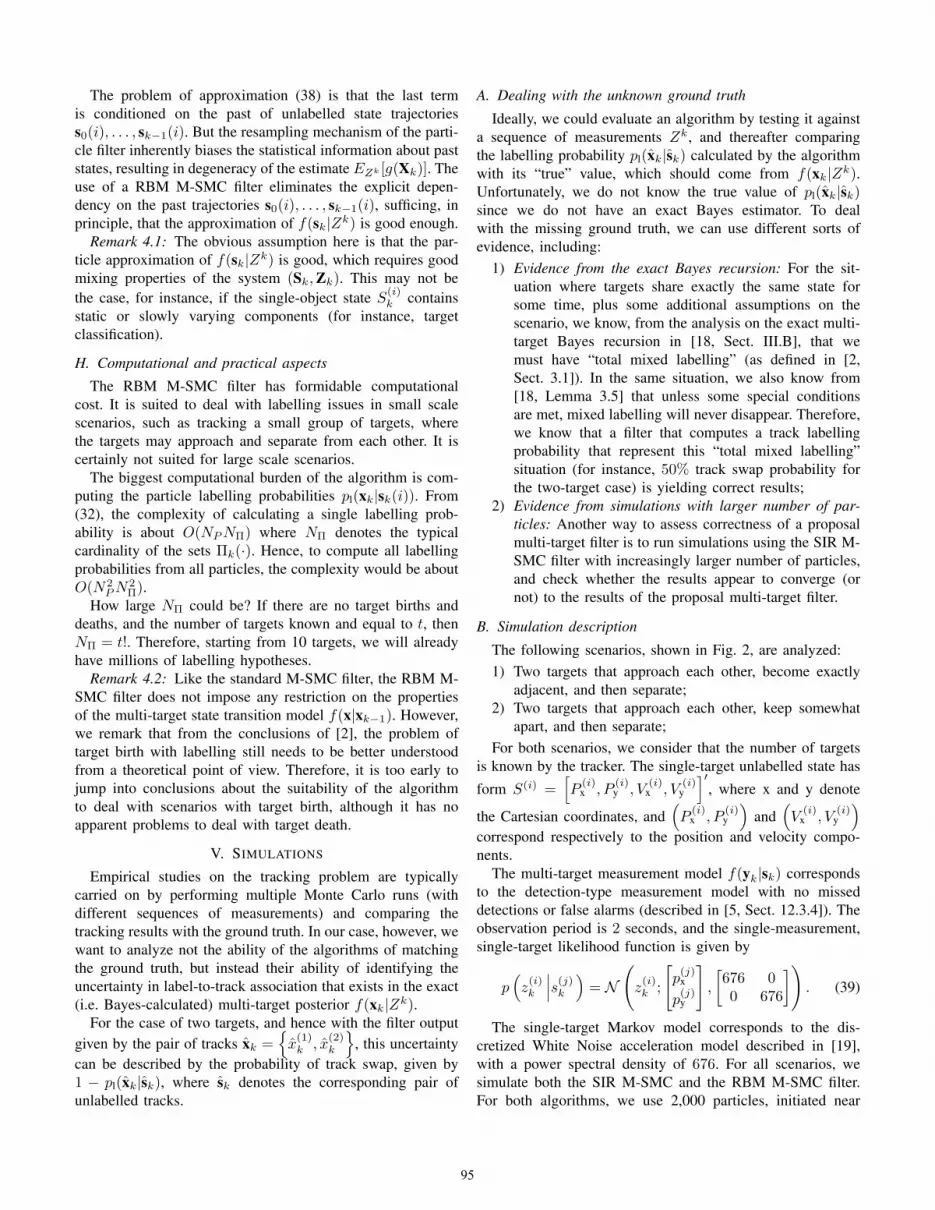
B. Simulation description

The following scenarios, shown in Fig. 2, are analyzed:

1) Two targets that approach each other, become exactly

adjacent, and then separate;

2) Two targets that approach each other, keep somewhat

apart, and then separate;

For both scenarios, we consider that the number of targets

is known by the tracker. The single-target unlabelled state has

form S(i) =[

P(i)x , P

(i)y , V

(i)x , V

(i)y

]′

, where x and y denote

the Cartesian coordinates, and(

P(i)x , P

(i)y

)

and(

V(i)

x , V(i)

y

)

correspond respectively to the position and velocity compo-

nents.

The multi-target measurement model f(yk|sk) corresponds

to the detection-type measurement model with no missed

detections or false alarms (described in [5, Sect. 12.3.4]). The

observation period is 2 seconds, and the single-measurement,

single-target likelihood function is given by

p(

z(i)k

∣

∣

∣s(j)k

)

= N

(

z(i)k ;

[

p(j)x

p(j)y

]

,

[

676 00 676

]

)

. (39)

The single-target Markov model corresponds to the dis-

cretized White Noise acceleration model described in [19],

with a power spectral density of 676. For all scenarios, we

simulate both the SIR M-SMC and the RBM M-SMC filter.

For both algorithms, we use 2,000 particles, initiated near

95

1000 2000 3000 4000 5000 6000 7000

1000

1500

2000

2500

3000

3500

4000

4500

X axis (m)

Y a

xis

(m)

(a) Scenario 1

1000 2000 3000 4000 5000 6000 7000

1000

1500

2000

2500

3000

3500

4000

4500

X axis (m)

Y a

xis

(m)

(b) Scenario 2

Fig. 2. Multi-target simulation scenarios

1000 2000 3000 4000 5000 6000 7000

1000

1500

2000

2500

3000

3500

4000

4500

X axis (m)

Y a

xis

(m)

(a) Scenario 1: MMOSPA-MLP using RBM

0 5 10 15 20 25 30 350

5

10

15

20

25

30

35

40

45

50

Time step

Tra

ck s

wap p

robabili

ty (

%)

SIR

SIR NPx10

RBM

(b) Scenario 1: Estimated track swap probabilities

1000 2000 3000 4000 5000 6000 7000

1000

1500

2000

2500

3000

3500

4000

4500

X axis (m)

Y a

xis

(m)

(c) Scenario 2: MMOSPA-MLP using RBM

0 5 10 15 20 25 30 350

5

10

15

20

25

30

35

40

45

50

Time step

Tra

ck s

wap p

robabili

ty (

%)

SIR

SIR NPx10

RBM

(d) Scenario 2: Estimated track swap probabilities

Fig. 3. Simulation results

the true locations of targets. Moreover, we will simulate an

additional run of the SIR M-SMC filter using 10 times more

particles, that we will henceforth refer as “SIR NP × 10”.

For both particle filters, we use the Markov density as

importance sampling function, i.e. f(xk(i)|xk−1(i)) for the

SIR M-SMC filter, and f(sk(i)|sk−1(j)) for the RBM M-SMC

filter.

C. Simulation results for each scenario

1) Scenario 1: Fig. 3(a) shows the MMOSPA-MLP esti-

mate calculated by the RBM M-SMC filter. Although this

run results in a track swap, we remark that the figure is only

included here for illustrative purposes; since this scenario rep-

resents a “total confusion” situation, we know, from evidence

1 of Section V-A, that the “true” probability of track swap is

around 50%; therefore, whether an algorithm produces or not

the correct assignment of labels for a single run is statistically

irrelevant. In the figure, the continuous lines correspond to

the true trajectories of targets, and the circles/squares denote

the MMOSPA-MLP tracks. For these tracks, each different

color/symbol combination corresponds to a different assigned

track label.

To compare the three algorithms, we will look instead at Fig.

3(b) that shows the track swap probabilities for the MMOSPA-

MLP estimates calculated by the three algorithms. Although

96

these probabilities are rigorously not comparable (since they

are not based on the same values of xk), nonetheless they

provide valuable information about the behavior of each filter.

Using evidence 1 of Section V-A, we can see that only

the RBM M-SMC results in the correct probability of track

swap of 50%. Clearly, both SIR M-SMC filters are affected by

the self-resolving phenomenon, with the ambiguity in label-

to-track association being severely underestimated. Note that,

as predicted from evidence 2, the SIR NP ×10 leads to better

results: its computed track swap probabilities are significatly

higher than the SIR. It is also easy to see, from Fig. 3(b), that

using a SIR with more particles only postpones, but does not

prevent, the self-resolving phenomenon.2) Scenario 2: Note that, since in this scenario there seems

to be only partial confusion of target statess, we cannot assess

correctness purely on basis of evidence 1. Let us then give

a close look at Fig. 3(d). We can see that, by increasing the

number of particles of the SIR M-SMC filter, the calculated

track swap probabilities become closer to the result of the

RBM M-SMC filter. Since from evidence 2, increasing the

number of particles of a SIR M-SMC filter should lead to

better accuracy, we can at least say that the RBM M-SMC

filter leads to more accurate track swap probabilities than the

SIR for the same number of particles.

Besides, the RBM M-SMC filter, unlike the SIR M-SMC fil-

ers, maintains the same track swap probability after the targets

separate. This behavior seems appropriate, since measurements

subsequent to target separation would not be informative w.r.t.

the true target identities. Hence, we can assess that the decline

of the track swap probability observed in the two SIR M-SMC

filters is due to self-resolving.

VI. CONCLUSION

In this paper over the MTTL problem, we followed our

theoretical discussion in [2] with the proposition of a novel

Sequential Monte Carlo solution for this problem. In order

to design this solution, we derived an extension of the Rao-

Blackwellized Marginal particle filter, that, we believe, may

also be useful for different applications. The experimental

results show that the proposed algorithm, the RBM M-SMC

filter, is indeed far more suitable to answering the questions

that we proposed in Section I (and were mathematically

formulated in [2]), than the “plain vanilla” particle filter

implementation of the MTTL problem, i.e. the SIR M-SMC

filter.

An interesting future work would be to evaluate (or adapt)

the algorithm for scenarios with target birth, but before doing

that, we plan first to give a better theoretical look at the

problem of target birth with labelling, as we mentioned in [2].

Another possible future work is to find adequate performance

measures for evaluating scenarios with only “partial mixed

labelling”, such that we can more precisely assess the accuracy

of labelling probabilities for such scenarios.

ACKNOWLEDGMENTS

The research leading to these results has received funding

from the EU’s Seventh Framework Programme under grant

agreement n 238710. The research has been carried out in

the MC IMPULSE project: https://mcimpulse.isy.liu.se.

This research has been also supported by the Netherlands

Organisation for Scientific Research (NWO) under the Casimir

program, contract 018.003.004. Under this grant Yvo Boers

holds a part-time position at the Department of Applied

Mathematics at the University of Twente.

We also thank Hans Driessen (Thales Nederland B.V.) for

the valuable contributions.

REFERENCES

[1] Y. Boers, E. Sviestins, and J. N. Driessen, “Mixed labelling in multitargetparticle filtering,” IEEE Trans. Aerosp. Electron. Syst., vol. 46, no. 2,pp. 792–802, 2010.

[2] E. H. Aoki, Y. Boers, L. Svensson, P. K. Mandal, and A. Bagchi,“A Bayesian look at the optimal track labelling problem,” in Proc.

DF&TT’12, London, UK, May 16–17, 2012.[3] B.-N. Vo, S. Singh, and A. Doucet, “Sequential Monte Carlo methods

for multitarget filtering with random finite sets,” IEEE Trans. Aerosp.

Electron. Syst., vol. 41, no. 4, pp. 1224–1245, 2005.[4] M. Vihola, “Rao-Blackwellised particle filtering in random set multitar-

get tracking,” IEEE Trans. Aerosp. Electron. Syst., vol. 43, no. 2, pp.689–705, 2007.

[5] R. Mahler, Statistical Multisource-Multitarget Information Fusion.Noorwood, MA: Artech House, 2007.

[6] D. B. Reid, “An algorithm for tracking multiple targets,” IEEE Trans.

Autom. Control, vol. AC-24, no. 6, Dec. 1979.[7] D. Crouse, P. Willett, L. Svensson, D. Svensson, and M. Guerriero, “The

set MHT,” in Proc. FUSION 2011, Chicago, IL, Jul. 5–8, 2011.[8] J. Vermaak, A. Doucet, and P. Perez, “Maintaining multi-modality

through mixture tracking,” in Proc. 9th IEEE International Conference

on Computer Vision, vol. 2, Nice, France, 2003, pp. 1110–1116.[9] H. A. P. Blom and E. A. Bloem, “Particle filtering for stochastic hybrid

systems,” in Proc. 43rd IEEE Conf. Decision and Control, Atlantis,Bahamas, Dec. 14–17, 2004.

[10] M. Briers, A. Doucet, and S. Maskell, “Smoothing algorithms for state-space model,” Annals Institute Statistical Mathematics, vol. 62, no. 1,pp. 61–89, 2010.

[11] A. Garcıa-Fernandez, M. Morelande, and J. Grajal, “Particle filterfor extracting target label information when targets move in closeproximity,” in Proc. FUSION 2011, Chicago, IL, Jul. 5–8, 2011.

[12] H. A. P. Blom and E. A. Bloem, “Decomposed particle filtering andtrack swap estimation in tracking two closely spaced targets,” in Proc.

FUSION 2011, Chicago, IL, Jul. 5–8, 2011.[13] F. Lindsten, T. B. Schon, and L. Svensson, “A non-degenerate Rao-

Blackwellised particle filter for estimating static parameters in dynam-ical models,” in Proc. 16th IFAC Symposium on System Identification

(SYSID), 2012.[14] C. Andrieu and A. Doucet, “Particle filtering for partially observed

Gaussian state space models,” J. Royal Stat. Soc. B, vol. 64, pp. 827–836, 2002.

[15] M. Klaas, N. de Freitas, and A. Doucet, “Toward practical N2 MonteCarlo: the marginal particle filter,” in Proc. 21th Conference Annual

Conference on Uncertainty in Artificial Intelligence (UAI-05). Arling-ton, Virginia: AUAI Press, 2005, pp. 308–315.

[16] E. H. Aoki, Y. Boers, L. Svensson, P. K. Mandal, and A. Bagchi,“An analysis of the Bayesian track labelling problem,” University ofTwente, Enschede, The Netherlands, Tech. Rep. 1980, 2012. [Online].Available: http://www.math.utwente.nl/publications

[17] D. Schuhmacher, B.-T. Vo, and B.-N. Vo, “A consistent metric forperformance evaluation of multi-object filters,” IEEE Trans. Signal

Process., vol. 56, no. 8, pp. 3447–3457, 2008.[18] E. H. Aoki, A. Bagchi, P. Mandal, and Y. Boers, “A theoretical analysis

of Bayes-optimal multi-target tracking and labelling,” University ofTwente, Enschede, The Netherlands, Tech. Rep. 1953, 2011. [Online].Available: http://www.math.utwente.nl/publications

[19] Y. Bar-Shalom, X. R. Li, and T. Kirubarajan, Estimation with applica-

tions to tracking and navigation. New York, NY: John Wiley & Sons,2001, ch. 6.

97