The relation of phase noise and luminance contrastto overt attention in complex visual stimuli

Division of Biology, California Institute of Technology,Pasadena, CA, USAWolfgang Einhauser

Computation and Neural Systems, California Institute of Technology,Pasadena, CA, USAUeli Rutishauser

Computation and Neural Systems, California Institute of Technology,Pasadena, CA, USAE. Paxon Frady

Institute of Cognitive Science, University of Osnabruck,Osnabruck, GermanySwantje Nadler

Institute of Cognitive Science, University of Osnabruck,Osnabruck, GermanyPeter Konig

Division of Biology, Division of Engineering andApplied Science, California Institute of Technology,

Pasadena, CA, USAChristof Koch

Models of attention are typically based on difference maps in low-level features but neglect higher order stimulus structure.To what extent does higher order statistics affect human attention in natural stimuli? We recorded eye movements whileobservers viewed unmodified andmodified images of natural scenes. Modifications included contrast modulations (resultingin changes to first- and second-order statistics), as well as the addition of noise to the Fourier phase (resulting in changes tohigher order statistics). We have the following findings: (1) Subjects’ interpretation of a stimulus as a ‘‘natural’’ depiction of anoutdoor scene depends on higher order statistics in a highly nonlinear, categorical fashion. (2) Confirming previous findings,contrast is elevated at fixated locations for a variety of stimulus categories. In addition, we find that the size of this elevationdepends on higher order statistics and reduces with increasing phase noise. (3) Global modulations of contrast bias eyeposition toward high contrasts, consistent with a linear effect of contrast on fixation probability. This bias is independent ofphase noise. (4) Small patches of locally decreased contrast repel eye position less than large patches of the sameaggregate area, irrespective of phase noise. Our findings provide evidence that deviations from surrounding statistics, ratherthan contrast per se, underlie the well-established relation of contrast to fixation.

Keywords: attention, eye movements, saliency, phase noise, higher order statistics, natural scenes, fractals

Introduction

When viewing complex stimuli, human observerssequentially shift their attention (James, 1890). In naturalvision, shifts in eye position correlate tightly with suchattentional shifts (Rizzolatti, Riggio, Dascola, & Umilta,1987). Various factors guide this ‘‘overt’’ attention, such asthe features of the stimulus, the observer’s experience, andthe task (Buswell, 1935; Yarbus, 1967). Most models ofhuman attention focus on the former ‘‘bottom–up’’ signals,resting upon the concept of a ‘‘saliency map’’ (Koch &Ullman, 1985). According to this scheme, stimuli areprocessed in multiple independent feature channels, localdifferences (‘‘contrasts’’) in these channels are summed,and the activity in the resulting saliency map reflects the

probability of a location to be attended. Various imple-mentations of the saliency-map scheme predict humanfixation behavior in natural scenes better than chance (Itti& Koch, 2000; Parkhurst, Law, & Niebur, 2002; Peters,Iyer, Itti, & Koch, 2005; Tatler, Baddeley, & Gilchrist,2005). One of the model’s featuresVluminance contrastVis elevated at fixation, as compared with random locations(Krieger, Rentschler, Hauske, Schill, & Zetzsche, 2000;Reinagel & Zador, 1999). This effect, however, is contin-gent on correcting for a general fixation bias toward theimage center (Mannan, Ruddock, & Wooding, 1996, 1997)or on restricting analysis to certain spatial frequencies(Einhauser & Konig, 2003; Tatler et al., 2005). In addition,this correlation does not imply a causal contribution of lumi-nance contrast to fixation but rather reflects the correlationof both with a higher order stimulus property (Einhauser &

Journal of Vision (2006) 6, 1148–1158 http://journalofvision.org/6/11/1/ 1148

doi: 10 .1167 /6 .11 .1 Received September 2, 2005; published October 9, 2006 ISSN 1534-7362 * ARVO

Konig, 2003). This raises the question to what extent theeffect of a low-level feature, such as luminance contrast, onattention depends on higher order stimulus statistics.

Several studies directly measure the effect of higherorder statistics on human attention. By analyzing bispec-tral densities, Krieger et al. (2000) find higher order‘‘structural differences’’ between fixated and nonfixatedregions. These authors propose two-dimensional imageproperties, like curves, edges, spots, and so forth, tounderlie the selection of fixation points. Privitera, Fujita,Chernyak, and Stark (2005) not only identify severalgeneric geometric kernels that are good predictors offixated regions but also stress that their results are onlyvalid for ‘‘generic’’ imagesVin their case, landscapes,interiors, and object collectionsVand in the absence of aspecific task. In earlier work (Privitera & Stark, 2000), thesame authors had compared 10 different algorithms forpredicting fixation locations in a variety of images. Theperformance of any algorithm depends largely on the im-age category: For example, while contrast is a good pre-dictor in ‘‘terrain’’ scenes, symmetry is more important inartistic paintings. Consequently, results on attention in‘‘natural’’ scenes have to be probed for such categorydependence.

The averaged amplitude spectra of natural scenes tend tofollow a 1/f law (Betsch, Einhauser, Kording, & Konig,2004; Field, 1987; Ruderman & Bialek, 1994; Torralba &Oliva, 2003; van der Schaaf & van Hateren, 1996). Mostinformation on the content of a specific natural scene,however, seems to be contained in its phase spectrum:When mixing the amplitude spectrum of one image withthe phase spectrum of another, the image contributing thephase dominates the perception of the mixture (Oppenheim& Lim, 1981). Adding noise to the phase of a stimulusmodulates responses in the visual cortex of macaquemonkeys (Rainer, Augath, Trinath, & Logothetis, 2001,but see Dakin, Hess, Ledgeway, & Achtman, 2002) andalso impairs their performance in a memory task (Rainer,Lee, & Logothetis, 2004). High levels of phase noise alsoimpair human performance in a rapid categorization task,but some category information is retained in the amplitudespectrum (Wichmann, Braun, & Gegenfurtner, 2006). Inthe context of overt attention, monkeys are less likelyto fixate areas of the stimulus that are locally deprived ofphase information, which can be compensated for by alocal increase in luminance contrast (Kayser, Nielsen, &Logothetis, 2006). Because monkey and human fixationsare affected differently by subtle local changes of lumi-nance contrast (Einhauser, Kruse, Hoffmann, & Konig,2006), it is unclear whether this result transfers to humanobservers.

We investigate how higher order stimulus statisticsinteract with a first-order feature in guiding human overtattention. To do so, we test the following questions:

1. Are higher order stimulus statistics needed for thesubjective perception of an outdoor scene as natural?

2. Does the elevation of luminance contrast at fixationsdepend on higher order statistics or stimulus category?

3. Do large-scale variations of luminance contrast biasattention irrespective of higher order statistics?

4. Do local variations of luminance contrast have similareffects as global changes?

We address these questions by measuring eye movementsof human observers while they view statistically modifiedimages of outdoor scenes, man-made objects, human faces,and fractals.

Methods

Stimuli

We performed four separate experiments using grayscaleimages. All experiments used outdoor images based on theZurich Natural Image Database (Einhauser et al., 2006;http://www.klab.caltech.edu/~wet/ZurichNatDB.tar.gz),which contain none or very few man-made objects. InExperiment 1, three additional categories were used:‘‘man-made objects’’ from the McGill calibrated colorimage database (Olmos A. and Kingdom F. A. A.),‘‘fractals’’ from the chaotic n-space network database(http://www.cnspace.net/html/fractals_gallery.html), andfrontal views of 16 different faces taken with a SonyDSC-V1 cybershot camera (Sony, Tokyo, Japan) undercontrolled lighting conditions (Figure 1a). In Experiments 1and 4, stimuli were used at a resolution of 1,024 �768 pixels and 8-bit grayscale; in Experiments 2 and 3,images were centrally cropped to 768 � 768 pixels.

Phase noise

To manipulate the higher order statistics of a stimulus, wemodified its phase spectrum. The amplitude spectrum wasunchanged. We transformed the original images to Fourierspace, added noise to the phases, and transformed thecombination of amplitude and phase back into image space.The additive noise was drawn from a normal distribution ofstandard deviationA (Experiments 2 and 3) or a symmetricuniform distribution of width ) (Experiments 1 and 4)and zero mean. To minimize the effects on overall contrastin the stimuli, in Experiments 1 and 4, we drew the noisefor only half of the Fourier coefficients at random andchose the other half as the respective complement topreserve the symmetry in coefficients. Figure 1b displaysexamples of such stimuli for two different levels of phasenoise.

Contrast gradients

To investigate the effect of global changes in luminancecontrast independently from other features in the image, weincreased or decreased luminance contrast gradually in the

Journal of Vision (2006) 6, 1148–1158 Einhauser et al. 1149

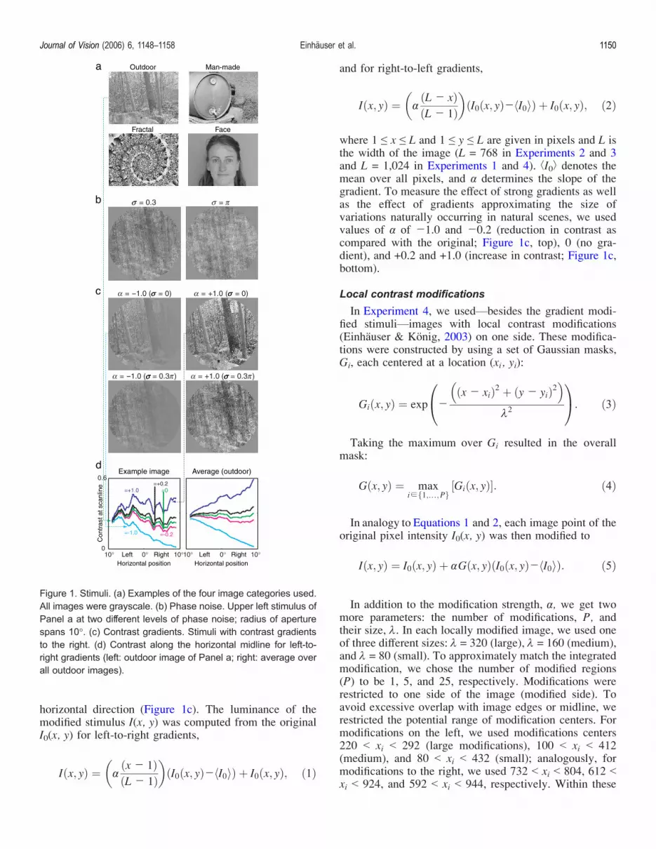
horizontal direction (Figure 1c). The luminance of themodified stimulus I(x, y) was computed from the originalI0(x, y) for left-to-right gradients,

I x; yð Þ ¼ !x j 1ð ÞðL j 1Þ

� �I0ðx; yÞj I0h ið Þ þ I0 x; yð Þ; ð1Þ

and for right-to-left gradients,

I x; yð Þ ¼ !L j xð ÞðL j 1Þ

� �I0ðx; yÞj I0h ið Þ þ I0 x; yð Þ; ð2Þ

where 1 e x e L and 1 e y e L are given in pixels and L isthe width of the image (L = 768 in Experiments 2 and 3and L = 1,024 in Experiments 1 and 4). bI0À denotes themean over all pixels, and ! determines the slope of thegradient. To measure the effect of strong gradients as wellas the effect of gradients approximating the size ofvariations naturally occurring in natural scenes, we usedvalues of ! of j1.0 and j0.2 (reduction in contrast ascompared with the original; Figure 1c, top), 0 (no gra-dient), and +0.2 and +1.0 (increase in contrast; Figure 1c,bottom).

Local contrast modifications

In Experiment 4, we usedVbesides the gradient modi-fied stimuliVimages with local contrast modifications(Einhauser & Konig, 2003) on one side. These modifica-tions were constructed by using a set of Gaussian masks,Gi, each centered at a location (xi, yi):

Gi x; yð Þ ¼ exp jðx j xiÞ2 þ ðy j yiÞ2� �

12

0@

1A: ð3Þ

Taking the maximum over Gi resulted in the overallmask:

Gðx; yÞ ¼ maxiZf1;I;Pg

Giðx; yÞ½ �: ð4Þ

In analogy to Equations 1 and 2, each image point of theoriginal pixel intensity I0(x, y) was then modified to

Iðx; yÞ ¼ I0ðx; yÞ þ !Gðx; yÞ I0ðx; yÞj I0h ið Þ: ð5Þ

In addition to the modification strength, !, we get twomore parameters: the number of modifications, P, andtheir size, 1. In each locally modified image, we used oneof three different sizes: 1 = 320 (large), 1 = 160 (medium),and 1 = 80 (small). To approximately match the integratedmodification, we chose the number of modified regions(P) to be 1, 5, and 25, respectively. Modifications wererestricted to one side of the image (modified side). Toavoid excessive overlap with image edges or midline, werestricted the potential range of modification centers. Formodifications on the left, we used modifications centers220 G xi G 292 (large modifications), 100 G xi G 412(medium), and 80 G xi G 432 (small); analogously, formodifications to the right, we used 732 G xi G 804, 612 Gxi G 924, and 592 G xi G 944, respectively. Within these

Figure 1. Stimuli. (a) Examples of the four image categories used.All images were grayscale. (b) Phase noise. Upper left stimulus ofPanel a at two different levels of phase noise; radius of aperturespans 10-. (c) Contrast gradients. Stimuli with contrast gradientsto the right. (d) Contrast along the horizontal midline for left-to-right gradients (left: outdoor image of Panel a; right: average overall outdoor images).

Journal of Vision (2006) 6, 1148–1158 Einhauser et al. 1150

ranges, the centers of the local modifications were ran-domly chosen so that no two modifications would be lessthan a distance 1 apart.

Definition of luminance contrast

In line with earlier studies (Reinagel & Zador, 1999) andas a canonic generalization of the two-point contrast, wedefined luminance contrast at each point of a stimulus asthe standard deviation of luminance in a patch divided bythe mean luminance of the stimulus. In the presentcontext, it is important to note that the global gradientsas described above do manipulate luminance contrastaccording to this definition. Figure 1d depicts the lumi-nance contrast measured along a horizontal scan line inan image modified with the different gradient strengths, !.It can be seen that local luminance contrast is dominatedby the gradient, on average. Hence, the definition ofluminance contrast used in the analysis of local featuresand the gradients is compatible. We based all analysis on apatch size of 80 � 80 pixels (2.1- � 2.1-), but results werequalitatively similar for a wide range of patch sizes.

Contrast at fixation/choice of baseline

We aim to test whether or not contrast is elevated atfixated locations, as compared with feature values measuredat randomly sampled locations (‘‘baseline locations’’).There are different possible means of choosing the baselinelocations. First, one can sample the image uniformly, that is,measure the feature value at or around each pixel. We willrefer to this sampling as ‘‘uniform baseline.’’ Comparingfixated locations to the uniform baseline, however, may besubject to a confound: Assume that the feature under inves-tigation is likely to be elevated at a certain region (say, thecenter). Assume further that fixations are generally biasedtoward this region. Then, even if the feature has no effecton fixation, comparison between fixated locations and uni-form baseline locations would show elevation of the fea-ture at fixated locations. Hence, we also compute a secondbaseline, which we sample at all locations fixated by thesubject when viewing all other stimuli of the same cate-gory and gradient level. Because these locations accountfor effects of general biases in fixated locations, we will re-fer to this sampling as ‘‘unbiased baseline’’ (for a thoroughdiscussion of central biases and the appropriate choice ofbaseline, see also Mannan et al, 1996; Tatler et al., 2005).Here, we report results relative to the unbiased baselinethroughout. Results were not qualitatively different for theuniform baseline.

Experimental design

Experiment 1 (stimulus categories)

In this experiment, we tested four different imagecategories (outdoor scenes, man-made objects, fractals,and faces). Each subject was shown two different, randomly

chosen images of each category, at 12 different phase-noiselevels, yielding a total of 2 � 4 � 12 = 96 trials per subject.Subjects were instructed to ‘‘study the images carefully.’’Each trial lasted 6 s and was preceded by a central fixationcue on medium-luminance background. After 50 trials, thecalibration of the eye-tracking system was validated and thesystem was recalibrated if needed. All but one subjectperformed one session (96 trials). For the lone subject whoperformed two sessions, only the first session was used foranalysis. Including the second session, however, did notqualitatively affect the results.

Experiment 2 (contrast gradients)

In this experiment, 10 outdoor scene images were pre-sented at 10 different levels of additive phase noise, yielding100 different stimuli. These stimuli were used without gra-dient (! = 0) and with four different gradient levels (! = j1.0,! = j0.2, ! = +0.2, and ! = +1.0) in two directions (fromleft to right and from right to left). The resulting 900 dif-ferent stimuli were distributed over nine blocks of 100 trials.Stimuli were balanced such that each of the 100 combina-tions of picture and phase-noise level appeared exactly withone type of gradient in each block.

Each trial started with a black central fixation cue on amedium-luminance (55 cd/m2) background that was displayedfor 0.5 s. Subsequently, the stimulus was presented for 2.5 s.After the offset of the stimulus, subjects had to indicate bypressing one of two mouse buttons ‘‘whether or not this im-age appears natural, i.e. resembles the image of a real-worldscene’’ (direct quotation from the written instructions givento the subject before the experiment). Following the sub-ject’s response, the next trial started immediately.

Before each block, the calibration of the eye-trackingdevice was validated and a new calibration was performed ifnecessary. Between blocks, subjects were allowed to takebreaks. Subjects performed three to five blocks in each re-cording session and needed two or three sessions to com-plete all of the nine blocks.

Experiment 3 (two-alternative forced-choiceexperiment)

This experiment used the same images and noise levels asExperiment 2. Ten different versions with different randompatterns of phase noise were generated for each of these100 conditions. The resulting 1,000 stimuli formed the targetset for the two-alternative forced-choice (2-AFC) experiment.

In each trial, 2 stimuli were presented in succession: 1 ofthe 1,000 target stimuli and 1 distracter that shared the sameamplitude spectrum but had random phase drawn from auniform distribution between j: and :. Each of the twostimuli was presented for 0.5 s and preceded by 0.5 s ofmedium-luminance blank screen. Subjects were asked toindicate, ‘‘which of the two stimuli looked more natural, i.e.more closely resembled the image of a real-world scene.’’

The order of trials was random throughout the experi-ment. The 1,000 trials were subdivided into 40 blocks of

Journal of Vision (2006) 6, 1148–1158 Einhauser et al. 1151

25 trials. After each block, there was a break of at leastabout 50 s, which subjects could extend as needed.

Experiment 4 (modification size)

In this experiment, we tested whether the effect of con-trast gradients was comparable to the effect of local con-trast modifications. We used 10 outdoor images (distinctfrom those used in Experiments 2 and 3) at the same modi-fication levels used in Experiment 2 (! = T1.0 and ! = T0.2).Besides the gradients, we used three different modificationsizes (large: 1 = 320, medium: 1 = 160, and small: 1 = 80).Because we were primarily interested in the effect of mod-ification size, we used only the two extreme phase-noiselevels: no noise and random phase. Instructions were iden-tical to Experiment 2. Using 10 images at two noise levels,two directions, four modification strengths, and four mod-ification sizes (gradients and three different 1), in additionto 10 images without contrast modification at two noise lev-els, yielded 660 trials. These were randomly ordered andsubdivided into 11 blocks of 60 trials, after each of whichsubjects could take a break when needed.

Presentation

Stimuli in all experiments were computed and displayedusing Matlab (MathWorks, Natick, MA) and its psycho-physics toolbox extension (Brainard, 1997; Pelli, 1997)running on a Windows PC.

1. In Experiment 1, stimuli were presented on a 21-in.CRT monitor (Samsung Electronics Co. Ltd., Korea)located 80 cm from the subject.

2. In Experiments 2 and 3, stimuli were presented on a19-in. CRT monitor (Sony, Tokyo, Japan), which waslocated 85 cm in front of the subject. Maximum lumi-nance (‘‘white’’) of the presentation screen was 110 cd/m2,whereas ambient light levels were below 0.01 cd/m2.The fringes of the stimuli were masked by a circularaperture with radius of 10- visual angle (L/2 = 384 pixels)to reduce any effects of screen boundaries. The back-ground outside the aperture had medium luminance(55 cd/m2). The gamma of the screen was corrected to en-sure a linear mapping from pixel values to displayedluminance.

3. In Experiment 4, we used a different monitor (DellInc., Round Rock, TX), whose maximum luminancewas 29 cd/m2 with otherwise identical settings toExperiments 2 and 3.

In all experiments, subjects’ heads were stabilized at constantdistance from the screen using a chin rest and a forehead rest.

Data acquisition

Throughout Experiments 1, 2, and 4, we recordedobservers’ eye positions using a noninvasive infrared eye

tracker. Experiment 1 used an Eyelink 2 system (SR ResearchLtd., Osgoode, ON, Canada); Experiment 2 used an ISCANETL-400 (ISCAN, Burlington, MA, USA), and Experiment 4used an Eyelink-1000 system. For the two Eyelink systems,we used the manufacturer’s software for calibration andvalidation and for determining periods of fixation. For theISCAN system, the mapping to screen coordinates wascomputed using a grid of 25 predefined fixation locationsas the bilinear transformation that minimizes the mappingerror for these data points. We determined fixations for theISCAN by using the algorithm developed by Peters et al.(2005; Peters, personal communication). We verified thatboth algorithms that determine fixations yield comparableresults on identical data sets.

Subjects

Fourteen volunteers (20 to 28 years old) from the Uni-versity of Osnabruck participated in Experiment 1. Thesame five volunteers from the Caltech Community (19 to28 years old) participated in Experiments 2 and 3. Five addi-tional volunteers from the Caltech Community (20 to 33 yearsold) participated in Experiment 4. All subjects had normalor corrected-to-normal vision, were naive as to the purposeof the experiment, and were paid or given course credit forparticipation. All experiments conformed to the Declara-tion of Helsinki and to the National and Institutional regu-lations for experiments with human subjects.

Results

Behavioral data: Are higher order statisticsneeded for perceiving scenes as natural?

First, we analyze to what extent the subjective perceptionof a stimulus as natural depends on phase noise (behavioralreports of Experiments 2, 3, and 4). In Experiment 2,subjects performed a yes/no paradigm. Images that did notundergo changes in their phase spectra (A = 0) were judgedas natural in almost all cases (99.4%, Figure 2a). Thisvalue decreased with increasing phase noise in a highlynonlinear fashion, which suggests a categorical rather thana continuous transition. It reached 9.0% for the maximumnoise level (A = :). This general behavior does not dependon the gradient strength ( p = .18, two-factor ANOVA onthe factors of noise level and gradient strength). Somesubjects, however, still reach relatively high values for A =: (maximum: 26%), which suggests that individuals mightemploy different criteria. During Experiment 4, when therewere only two noise levels (no noise and random phase), ob-servers showed the same pattern of responses: They judgedthe no-noise stimuli almost always natural (98.4% T 1.4%natural [M T SD]) and the random-phase stimuli ‘‘non-natural’’ (2.9% T 2.4% natural). To obtain a criterion-free

–

–

–

Journal of Vision (2006) 6, 1148–1158 Einhauser et al. 1152

measurement, we used a 2-AFC paradigm in Experiment 3.The subjects of Experiment 2 had to report which of the fol-lowing images they found more natural: one with varying Aor one with random phase (A Y V). For A = 0, subjectsalmost always (98.2%) correctly judge the image with lessphase noise as ‘‘more natural.’’ This performance decreasesagain in a sigmoidal fashion, becoming indistinguishablefrom chance level for A Q 0.6: (t test: p = .41 for A = 0.6:and p = .22 for A = :, Figure 2b). These data demonstratethat the subjective perception of an outdoor scene as naturalis contingent on higher order stimulus statistics and that thetransition between the two categories is sharp.

Does the relation between contrast andfixation depend on higher order statistics?

As first analysis of eye-movement data, we tested to whatextent the relation of luminance contrast to fixation dependson higher order statistics (Experiment 1). We tested 12levels of phase noise and four different stimulus catego-ries: outdoor scenes, fractals, man-made objects, andfaces. For stimuli without noise, the mean luminancecontrast was elevated at fixated locations relative tobaseline in all categories (outdoor scenes: 0.9% T 0.6%;fractals: 7.2% T 2.6%; man-made objects: 6.8% T 5.0%;faces: 2.9% T 1.5%, relative elevation over unbiasedbaseline, expressed as M T SEM across subjects, Figure 3).For all categories, the mean elevation across noise levelsis significantly larger than 0 (p = .001, p = 2 � 10j4, p = .01,p = .005, t tests for the individual categories pooled overnoise levels). However, the elevation decreases with increas-ing phase noise, and its size is significantly anticorrelated to), the amount of noise (r = j.95, p = 3 � 10j6; r = j.63,p = .03; r = j.89, p = 1 � 10j4; r = j.83, p = 9 � 10j4

for the four categories). The results of Experiment 1 con-firm the elevation of luminance contrast at fixated loca-tions for a variety of complex stimuli. They furthermoredemonstrate a dependence of this correlative effect on higherorder statistics. This is first evidence that a higher order

property related to contrast might contribute to the eleva-tion of contrast at fixated locations.

Do contrast gradients bias fixation?

Next, we measured the extent to which large-scale con-trast gradients bias observers’ eye position (Experiment 2).For each 2.5-s trial, we measured the median horizontaleye position over the whole trial, irrespective of the typeof eye movement (fixation, saccade, etc.). For images with-out any gradient (! = 0), the mean eye position is 0.02- T0.8- (M T SD over subjects) right of the center, which isnot a significant bias ( p = .96, t test). Large positive gra-dients (! = +1) introduce a strong bias toward the sideof higher contrast, which is significant for left-to-rightgradients (0.86- T 0.42- to the right, p = .01, Figure 4a)and shows the same tendency for right-to-left gradients(0.96- T 1.07- to the left, p = .11). The tendency is pre-served for small gradients ! = +0.2, which bias the eyeposition 0.25- T 0.54- and 0.24- T 0.94- in the direction ofthe gradient, although the effect is not significant for thisgradient strength ( p = .36 and p = .60, respectively). Fornegative gradients, we observe a similar effect: The biasalways goes in the direction of the higher contrast,yielding significant biases of 1.64- T 1.12- ( p = .03) and0.99- T 0.77- ( p = .04) for ! = j1.0 as well as similarnonsignificant tendencies for ! = j0.2 (0.35- T 0.73- and0.21- T 0.91-, p = .35 and p = .64, respectively, Figure 4a).Although the bias is not significant for shallow gradients,the gradient biases observers’ eye position toward highercontrasts in all cases. To quantify this effect further, wemeasure the difference between the biases in eye positionfor opposing gradients for each subject and for each gra-dient strength ! (Figure 4b). Over subjects, this differenceis significantly different from 0 for all but one ! ( p = .01,p = .01, p = .12, and p = .008 [t tests] for ! = j1.0, ! = j0.2,

Figure 2. Behavioral data. (a) Percentage of ‘‘yes’’ responses onwhether or not an image is natural in Experiment 2 versus phase-noise level. (b) Percentage correct (image with less phase noiseis judged more natural) in Experiment 3 versus phase-noise level.In both panels, error bars denote the standard error of the meanover the n = 5 subjects.

Figure 3. Elevation of contrast at fixations. Luminance contrastat fixations relative to unbiased baseline (see Methods section).(a) Outdoor scenes, (b) fractals, (c) man-made objects, (d) faces.All data are expressed as mean and standard error of the meanover subjects and best linear regression.

Journal of Vision (2006) 6, 1148–1158 Einhauser et al. 1153

! = +0.2, and ! = +1.0, respectively) and is highly signif-icantly correlated to ! (r = .99, p = .007).

In the Appendix, we analytically derive that a linear re-lation of fixation probability to contrast is consistent withthis linear correlation. In summary, the contrast gradienteffectively biases eye position toward regions of higher con-trasts, consistent with a linear relation of fixation proba-bility and luminance contrast.

Does the fixation bias induced by contrastgradients depend on higher order statistics?

Next, we investigate the extent to which the biases in-duced by first-order features depend on higher order sta-

tistics. Grouping the eye-tracking data by the response of thesubject reveals no difference between natural (Figure 4b,green) and nonnatural images (Figure 4b, red): Neither isthere any difference for any ! (p = .81, p = .22, p = .86,and p = .66) nor is the correlation between eye-positiondifference and ! affected (natural: r = .98, p = .02; non-natural: r = .995, p = .005). In addition to the binary group-ing in natural and nonnatural images, we also analyze howthe effect of contrast gradients depends on the phase-noiselevel. We do not find any significant correlation betweenthe effect of the contrast gradient on eye position andphase noise for any ! (! = j1.0: r = .23, p = .53; ! =j0.2: r = .03, p = .94; ! = +0.2: r = j.10, p = .78; ! =+1.0: r = .39, p = .26; Figure 4c). The same pattern ofresults is found when performing the analysis for periodsof fixations only (data not shown). In conclusion, the effectof the contrast gradient on eye position is significant andlinear in the gradient strength !. In addition, it is indepen-dent of whether or not the stimulus is judged as natural.

Do local contrast modifications have thesame effect as large-scale gradients?

Although we find that contrast reductions repel eyeposition in this study, earlier studies (Einhauser & Konig,2003; Einhauser et al., 2006) had demonstrated that stronglocal reductions of contrast have an attractive effect.Although these findings themselves stand undisputed, theirinterpretation has spurred controversy (Kayser et al., 2006;Parkhurst & Niebur, 2004). Consequently, we testedwhether the size of the modifications reconciles thesefindings (Experiment 4). Consistent with the data ofExperiment 2, contrast gradients biased observers to theside of high contrast. This bias had a trend to linearcorrelation with ! (r = .94, p = .07) and was independentof phase noise for all ! (t tests: p = .99, p = .99, p = .12,and p = .72 for ! = j1, ! = –0.2, ! = 0.2, and ! = 1,respectively). As with the gradients, there is no significantdifference between no-noise and random-phase stimuli atany modification level or modification size ( p 9 .19 for allt tests for ! and 1). For all three sizes, the bias depends onmodification level (large: p = .002, medium: p = .001,small: p = .004, ANOVA). However, a significant linearcorrelation with modification level is observed only forthe largest modification size (r = .98, p = .02, Figure 5a)but not for medium (r = .92, p = .08, Figure 5b) or small(r = .80, p = .20, Figure 5c) modification. Furthermore, forthe small and medium modifications, the dependence on! is not monotonic, with strong negative modifications(! = j1.0) being less repulsive than moderate ones (! =j0.2). Finally, small, strongly negative modificationsareVif anythingVattractive (M T SD: 0.01- T 0.59- to-ward modified side). These results are in line with earlierdata on local modifications and make it conceivable thatstrong modifications assume an object-like quality that at-tracts attention, counteracting the otherwise repulsive ef-fect of low contrast.

Figure 4. Effect of contrast gradients. (a) Horizontal eye position intrials with gradients from left to right (gray) and gradients fromright to left (black) for different gradient strengths !. 0- denotescenter of screen. (b) Difference between horizontal eye position intrials with left-to-right gradients and right-to-left gradients for allstimuli (black), stimuli that subjects judged to be natural (green),and stimuli that they judged nonnatural (red). Lines denote corre-sponding optimal linear fit. (c) Difference between horizontal eyepositions between left-to-right and right-to-left gradient trials ver-sus phase-noise level. Different colors denote different gradientstrengths. All panels show mean and standard error of the meanover subjects.

Journal of Vision (2006) 6, 1148–1158 Einhauser et al. 1154

Discussion

In this study, we investigate how higher order stimulusstatistic modulates the effect of contrast on fixation. Wedemonstrate that

1. The perception of an outdoor scene as natural iscontingent on higher order stimulus statistics.

2. For a variety of categories, luminance contrast iselevated at fixated locations. This elevation is anti-correlated to phase noise and, thus, depends on higherorder statistics.

3. Global modifications of luminance contrast (gra-dients) attract attention if contrast is increased andrepel attention if contrast is decreased. This effect isindependent of higher order statistics.

4. The repulsive effect of decreased contrast vanishes orreverses for local modifications.

In summary, luminance contrast biases attention aspredicted by bottom–up models. However, to explain thelocal effects of contrast in natural scenes in full, one needs toconsider correlations to higher order statistics.

The predominant sensory-driven (bottom–up) model ofhuman attention, the saliency map (Itti, Koch, & Niebur,1998; Koch & Ullman, 1985), is based on difference maps(contrasts) in first-order features, such as luminance. Suchsaliency maps predict human fixation locations signifi-cantly above chance (Itti & Koch, 2000; Parkhurst et al.,2002; Peters et al., 2005; Tatler et al., 2005). However,their predictions are still far from the theoretical optimumfor bottom–up modelsVthe mutual prediction of scan pathsbetween different observers (Oliva, Torralba, Castelhano,& Henderson, 2003; Peters et al., 2005; Privitera et al.,2005). In line with the present results, this suggests that in-corporating relations to higher order statistics may improvesuch bottom–up models.

Two approaches exist to incorporate higher orderstatistics into bottom–up models. First, one may select a

different set of features than the classical saliency map,which explicitly or implicitly include higher order effects:Among the popular choices, there are edge density (Mannanet al., 1996); localized edges, corners, and points (Kriegeret al., 2000); ‘‘texture contrast’’ (Parkhurst & Niebur,2004, see below); and localized generic geometricalkernels (Privitera et al., 2005). Alternatively, one maylearn the relevant features from scene statistics. Such alearning approach comes at the advantage that it can bespecific to an image category (Torralba, 2003; Torralba &Oliva, 2003), which modulates at least effects of somelow-level features (Parkhurst et al., 2002) and simplegeometric properties like symmetry (Privitera & Stark,2000). Learning approaches can furthermore readily beextended to incorporate task-specific priors, that is, top–down knowledge (Navalpakkam & Itti, 2005; Oliva et al.,2003; Torralba, 2003). Irrespective of the preferredmodeling approach, our present findings highlight theimportance of higher order structure for the effect of alow-level featureVluminance contrast.

Several studies have investigated the relation of lumi-nance contrast to human attention in natural stimuli. Most ofthese studies find that luminance contrast is elevated atfixated locations (Einhauser & Konig, 2003; Krieger et al.,2000; Mannan et al., 1997; Reinagel & Zador, 1999;Tatler et al., 2005). The range of effects we observe here isconsistent with these results, when taking into accountsystematic biases of observers and images, as done in thisstudy (see Mannan et al., 1996; Tatler et al., 2005, for athorough discussion of this issue). Consequently, weconfirm earlier studies in describing a small, thoughsignificant, elevation of luminance contrast at fixatedlocations.

In an earlier study (Einhauser & Konig, 2003), we haddemonstrated that local reductions of luminance contrastattract attention. Consequently, the elevation of luminancecontrast at fixations is not a consequence of contrast itself.Instead, the elevation of contrast at fixation is theconsequence of their mutual correlation to a higher orderproperty. This interpretation is in line with the presentdata, in which contrast elevation anticorrelates with noiselevel; that is, it is at least partly dependent on higher orderstatistics.

Using a modified saliency-map model, Parkhurst andNiebur (2004) argued that a measure of contrast variation,which they dubbed texture contrast, is elevated whencontrast is locally decreased. Assuming texture contrast tobe 10-fold more attractive than luminance contrast, theirmodel indeed reproduced some aspects of the Einhauserand Konig (2003) data. The fact that contrast gradientsand large modifications bias attention to high contrasts,where small negative modifications have no such repul-sive effect (Experiment 4), provides an alternative explan-ation: Strong local negative modifications deviate from thelocal surrounding. Thereby, they stick out as an odd item,much like isolated features in pop-out (Treisman &Gelade, 1980). In the temporal domain, such local

Figure 5. Eye-position biases induced by local modifications ofdifferent size. Difference between horizontal eye position in trialswith modifications on the right and on the left; black: all stimuli;green: no noise; red: random phase. (a) Large modification (1 =320); (b) medium modification (1 = 160); (c) small modification(1 = 80).

Journal of Vision (2006) 6, 1148–1158 Einhauser et al. 1155

deviations from global context or expectation, recentlyformalized as Bayesian ‘‘surprise’’ (Itti & Baldi, 2005),also attract attention. Hence, it is well conceivable thatstrong negative modifications form a deviation fromcontext and, therefore, attract attention, counteracting therepulsive effect of reduced contrast. This view and thetexture-contrast interpretation of Parkhurst and Nieburare not mutually exclusive. On the contrary, texture con-trast forms one possible formalization of this concept,which also highlights the relative importance of higherorder stimulus statistics for the local guidance of overtattention.

Appendix

Linear model for contrast biases

Here, we demonstrate how the assumption that contrasthas a linear effect on fixation probability results in the biasinduced by gradients to be linear in gradient strength !. Theconditional probability to fixate a contrast c is given as

pðfixkcontrast ¼ cÞ ¼ .cþ n; ðA1Þ

where n is a normalization constant and . parameterizesthe effect of contrast on fixation. For simplicity, weconsider here only left-to-right gradients. Assuming thatthe gradient of strength ! dominates the average contrastposition x (Figure 1d), the contrast c(x) is given as

c xð Þ ¼ c0 !x

Lþ 1

� �; ðA2Þ

where L is the length of the image and c0 is theunmodified contrast (Figure 1d). The probability to fixatea certain contrast is

pðfix; cÞ ¼ pðcÞpðfixkcÞ: ðA3Þ

Under Equation A2, the prior for a contrast to be inthe image is uniform in [c0, (! + 1)c0] for positive ! (or in[(! + 1)c0, c0] for negative !) and 0 outside:

p cð Þ ¼

1

j!jc0

c0 G c G !þ 1ð Þc0

1

j!jc0

c0 9 c 9 !þ 1ð Þc0

0 otherwise

:

8>>>>>><>>>>>>:

ðA4Þ

Assuming all fixations are on the image, we have

p fix; cð Þ ¼ 1

j!jc0

.cþ nð Þ; ðA5Þ

with p being a probability we get for the constant n, forpositive !

1 ¼Z!þ1ð Þc0

c0

pðfix; cÞdc

¼ 1

!c0

�.

2c2

� !þ1ð Þc0

c0

þ nc½ � !þ1ð Þc0

c0

!

¼ .c0

!

2þ 1

� �þ n

!

¼ 1j .c0

!

2þ 1

� �: ðA6Þ

By interchanging the lower and upper integration limitsand replacing ! by j! in the normalization, we obtain thesame result for negative !. Hence, we expect the fixatedcontrast (again, the notation assumes positive !, but ex-changing the integration limits and replacing ª!ª = j!in the normalization yields the same result for negative !)to be

ch i ¼Z!þ1ð Þc0

c0

cpðfix; cÞdc

¼ .

!c0

Z!þ1ð Þc0

c0

c2dcþ 1

!c0

Z!þ1ð Þc0

c0

cdcj.

!

�!

2þ 1

� Z!þ1ð Þc0

c0

cdc

¼ .c20 !2

12þ c0

�1 þ !

2

�: ðA7Þ

Plugging this result into Equation A2, we obtain the meaneye position to be expected for gradient ! as

ch i ¼ cðx!Þ

¼ c0 !x!Lþ 1

� �

Á x! ¼ L

!

ch ic0

j1

� �

¼ L

!

.c20 !2

12c0

þ c0

c0

1 þ !

2

� �j1

� �

¼ L.c0!

12þ L

2: ðA8Þ

Á n

Journal of Vision (2006) 6, 1148–1158 Einhauser et al. 1156

Analogous to the above calculation, for right-to-left gra-dients, one obtains

Á x! ¼L

2j

L.c0!

12: ðA80Þ

This implies that a gradient extending over the wholeimage biases fixation by a fraction

.c0!

12ðA9Þ

of the image width L, relative to the image center (L/2) inthe direction of the gradient. This analytical result has twoimportant consequences: If one assumes a linear model forthe effect of contrast (or any feature) on fixation proba-bility and the gradient is sufficiently strong (compared withthe naturally occurring variation of the feature), one pre-dicts that

1. The induced position bias is linear in the gradientstrength,

2. A gradient in one direction of strength ! has an equiv-alent effect to the opposing gradient of strength j!.

Both predictions are consistent with our observations forgradients.

Acknowledgments

This work was supported by the Swiss National ScienceFoundation (W.E., Grant Nos. PBEZ2-107367 and PA00A-111447), NIMH, NGA, NSF, and Caltech’s ‘‘SURF’’program. We thank A. Acik and H.-P. Frey for technicalassistance and C. Quigley for editorial assistance.

Commercial relationships: none.Corresponding author: Wolfgang Einhauser.Email: wet@klab.caltech.edu.Address: CIT 216-76, 1200 E. California Blvd., Pasadena,CA 91125, USA.

References

Betsch, B. Y., Einhauser, W., Kording, K. P., &Konig, P. (2004). The world from a cat’s pers-pectiveVStatistics of natural videos. BiologicalCybernetics, 90, 41–50. [PubMed]

Brainard, D. H. (1997). The Psychophysics Toolbox.Spatial Vision, 10, 433–436. [PubMed]

Buswell, G. T. (1935). How people look at pictures. Astudy of the psychology of perception in art. Chicago,IL: The University of Chicago Press.

Dakin, S. C., Hess, R. F., Ledgeway, T., & Achtman,R. L. (2002). What causes non-monotonic tuning offMRI response to noisy images? Current Biology, 12,R476–R477. [PubMed] [Article]

Einhauser, W., & Konig, P. (2003). Does luminance-contrast contribute to a saliency map for overt visualattention? European Journal of Neuroscience, 17,1089–1097. [PubMed]

Einhauser, W., Kruse, W., Hoffmann, K. P., & Konig, P.(2006). Differences of monkey and human overt atten-tion under natural conditions. Vision Research, 46,1194–1209. [PubMed]

Field, D. J. (1987). Relations between the statistics ofnatural images and the response properties of corticalcells. Journal of the Optical Society of America A,Optics, Image Science, and Vision, 4, 2379–2394.[PubMed]

Itti, L., & Baldi, P. (2005). A principled approach todetecting surprising events in video. Proceedings ofthe IEEE Conference on Computer Vision andPattern Recognition (CVPR) (vol. 1, pp. 631–637).

Itti, L., & Koch, C. (2000). A saliency-based search mech-anism for overt and covert shifts of visual attention.Vision Research, 40, 1489–1506. [PubMed]

Itti, L., Koch, C., & Niebur, E. (1998). A model ofsaliency-based visual attention for rapid scene anal-ysis. IEEE Transactions on Pattern Analysis andMachine Intelligence, 20, 1254–1259.

James, W. (1890). Principles of psychology. New York: Holt.

Kayser, C., Nielsen, K. J., & Logothetis, N. K. (2006).Fixations in natural scenes: Interaction of imagestructure and image content. Vision Research, 46,2535–2545. [PubMed]

Koch, C., & Ullman, S. (1985). Shifts in selective visualattention: towards the underlying neural circuitry. HumanNeurobiology, 4, 219–227. [PubMed]

Krieger, G., Rentschler, I., Hauske, G., Schill, K., &Zetzsche, C. (2000). Object and scene analysis bysaccadic eye-movements: An investigation with higher-order statistics. Spatial Vision, 13, 201–214. [PubMed]

Mannan, S. K., Ruddock, K. H., & Wooding, D. S. (1996).The relationship between the locations of spatial featuresand those of fixations made during visual examinationof briefly presented images. Spatial Vision, 10, 165–188.[PubMed]

Mannan, S. K., Ruddock, K. H., & Wooding, D. S. (1997).Fixation patterns made during brief examination oftwo-dimensional images. Perception, 26, 1059–1072.[PubMed]

Navalpakkam, V., & Itti, L. (2005). Modeling the influenceof task on attention. Vision Research, 45, 205–231.[PubMed]

Journal of Vision (2006) 6, 1148–1158 Einhauser et al. 1157

Oliva, A., Torralba, A., Castelhano, M. S., & Henderson,J. M. (2003). Top–down control of visual attention inobject detection. IEEE Proceedings of the Interna-tional Conference on Image Processing, 1, 253–256.

Oppenheim, A. V., & Lim, J. S. (1981). The importanceof phase in signals. Proceedings of the IEEE, 69,529–541.

Parkhurst, D., Law, K., & Niebur, E. (2002). Modeling therole of salience in the allocation of overt visualattention. Vision Research, 42, 107–123. [PubMed]

Parkhurst, D., & Niebur, E. (2004). Texture contrast attractsovert visual attention in natural scenes. The EuropeanJournal of Neuroscience, 19, 783–789. [PubMed]

Pelli, D. G. (1997). The VideoToolbox software for visualpsychophysics: Transforming numbers into movies.Spatial Vision, 10, 437– 442. [PubMed]

Peters, R. J., Iyer, A., Itti, L., & Koch, C. (2005).Components of bottom–up gaze allocation in naturalimages. Vision Research, 45, 2397–2416. [PubMed]

Privitera, C. M., Fujita, T., Chernyak, D., & Stark, L. W.(2005). On the discriminability of hROIs, human visu-ally selected regions-of-interest. Biological Cybernetics,93, 141–152. [PubMed]

Privitera, C. M., & Stark, L. W. (2000). Algorithms fordefining visual regions-of-interest: Comparison witheye fixations. IEEE Transactions on Pattern Analysisand Machine Intelligence, 22, 970–982.

Rainer, G., Augath, M., Trinath, T., & Logothetis, N. K.(2001). Nonmonotonic noise tuning of BOLD fMRIsignal to natural images in the visual cortex of theanesthetized monkey. Current Biology, 11, 846–854.[PubMed]

Rainer, G., Lee, H., & Logothetis, N. K. (2004). Theeffect of learning on the function of monkeyextrastriate visual cortex. PLoS Biology, 2, E44.[PubMed] [Article]

Reinagel, P., & Zador, A. (1999). Natural scene statisticsat the centre of gaze. Network, 10, 341–350.[PubMed]

Rizzolatti, G., Riggio, L., Dascola, I., & Umilta, C.(1987). Reorienting attention across the horizontaland vertical meridians: Evidence in favor of apremotor theory of attention. Neuropsychologia, 25,31–40. [PubMed]

Ruderman, D. L., & Bialek, W. (1994). Statistics ofnatural images: Scaling in the woods. PhysicalReview Letters, 73, 814–817. [PubMed]

Tatler, B. W., Baddeley, R. J., & Gilchrist, I. D. (2005).Visual correlates of fixation selection: Effects ofscale and time. Vision Research, 45, 643 – 659.[PubMed]

Treisman, A. M., & Gelade, G. (1980). A feature-integration theory of attention, Cognitive Psychology,12, 97–136. [PubMed]

Torralba, A. (2003). Modeling global scene factors inattention. Journal of the Optical Society of AmericaA, Optics, Image Science, and Vision, 20, 1407–1418.[PubMed]

Torralba, A., & Oliva, A. (2003). Statistics of naturalimage categories. Network: Computation in NeuralSystems, 14, 391– 412. [PubMed]

van der Schaaf, A., & van Hateren, J. H. (1996).Modelling the power spectra of natural images:Statistics and information. Vision Research, 36,2759–2770. [PubMed]

Wichmann, F. A., Braun, D. I., & Gegenfurtner, K. R.(2006). Phase noise and the classification of naturalimages. Vision Research, 46, 1520–1529. [PubMed]

Yarbus, A. L. (1967). Eye movements and vision (B. Haigh,Trans.). New York: Plenum.

Journal of Vision (2006) 6, 1148–1158 Einhauser et al. 1158