The relationship between risk and incomplete states uncertainty: a Tsallis entropy perspective

Algorithmic Finance 2 (2013) 141–150 141DOI 10.3233/AF-13022IOS Press

The relationship between risk and incompletestates uncertainty: a Tsallis entropyperspectiveOren J. Tapiero1,2

Université Paris 1 Panthéon-Sorbonne (LabEx-ReFi), Paris, FranceTel-Aviv Academic College, Tel-Aviv, Israel

Abstract. This paper provides a “non-extensive” information theoretic perspective on the relationship between risk andincomplete states uncertainty. Theoretically and empirically, we demonstrate that a substitution effect between the latter twomay take place. Theoretically, the “non-extensive” volatility measure is concave with respect to the standard (based on normaldistribution) volatility measure. With the degree of concavity depending on an incomplete states uncertainty parameter-theTsallis-q. Empirically, the latter negatively causes the normal measure of volatility, positively affecting the tails of the distributionof realised log-returns.

Keywords: Tsallis Entropy, Incomplete Statistics, Volatility, Uncertainty.

Introduction

Financial risk models seek to accommodate uncer-tainty, which is distinct of the notion of risk (Knight,1921). In other words, they seek to account implicitlyfor ex-ante unknown future realisations (risks) andtheir associated probabilities (uncertainty). Classicalmodels, however, have confused uncertainty withrisk. Schinckus (2009) explains the latter confusionwith the adoption of expected utility theory (EU) asa principal framework for analysing decision making

1Email Address: [email protected]: The author is grateful to comments

made to this paper by Prof. Phil Maymin (Polytechnic Instituteof New York University), Prof. Raphael Douady (CNRS andUniversity of Paris 1, Department of Economics, France), Prof.Dominique Guégan (CNRS and University of Paris 1, Departmentof Economics, France), Prof. Yaffa Machnes (Bar-Ilan University,Graduate School of Business and Administration, Israel), Prof. GilaFruchter (Bar-Ilan University, Graduate School of Business andAdministration, Israel), Prof. Jeremy Schiff (Bar-Ilan University,Department of Mathematics, Israel), Dr. Shlomit Zuta (Tel Aviv-Yaffo Academic College) and Prof. Tamir Agmon (Tel Aviv-YaffoAcademic College).

under uncertainty. Its underlying principal is that“objective” probabilities can be estimated when the setof future realisations (or states) is a-priori complete.Hence, classical risk measures confound risk withuncertainty.

Critics of the EU framework, such as Ellsberg(1961), point to the difficulty of estimating these“objective” probabilities when the set of future statesis a-priori incomplete. Therefore, generalisations ofthe EU have sought to accommodate for an addeduncertainty due to incomplete ex-ante knowledge offuture states. This is done usually by “distorting” the“objective” probabilities. For example, the prospecttheory (PT) of Kahneman and Tversky (1979)introduce a value function that overweight stateswith small probabilities. The anticipated utility theory(AUT) of Quiggin (1982) distorts probabilities as inPT, but by distorting the probability density functionas whole and not individually like in PT. Tverskyand Kahneman (1992) extends the PT and AUT tothe Cumulative PT by allowing probabilities to bejointly weighted without not violating the transitivityaxiom (as is the case of AUT). Further examples of

2158-5571/13/$27.50 c© 2013 – IOS Press and the authors. All rights reserved

142 O.J. Tapiero / The relationship between risk and incomplete states uncertainty: a Tsallis entropy perspective

using “distorted” probabilities also include: Karmarkar(1978), Chew and MacCrimmon (1979) and Gul(1991).

In general, uncertainty is a notion that relates towhat is unknown, or non quantifiable or uninsurable(see: LeRoy and Singell (1987), Langlois and Cosgel(1993) and Schinckus (2009) for further discussion).Nevertheless, statistical mechanics and informationtheory (Shannon, 1948; Jaynes, 1957) provide a modelto circumvent uncertainty (based on Laplace principleof insufficient reason) using entropy functions. InBoltzmann (1878), entropy (or expected uncertainty)depends only on the normal standard deviation (orvolatility – σ1) which in finance is used as measureof risk. In that sense, volatility summarises bothrisk (future realisation is unknown) and uncertainty(unknown probabilities). However, it is unable toaccount for possible incompleteness of the set offuture states, which renders the task of estimatingprobabilities even more difficult.

In this paper, two parameters determine overalluncertainty: the Tsallis parameter q and a “non-extensive” measure of risk (or standard deviation) –σq . The first parameter relates to the added uncertaintydue to suspected incomplete knowledge of futurestates. The second is shown to be concave with respectto the normal standard deviation and vanishes whenq tends to its limit (at q = 3). This suggests that asubstitution effect may take place between risk (σq andσ1) and incomplete states uncertainty (q).

This incomplete states uncertainty (implied fromhistorical log-returns of the S&P-500) is shown tobe exclusively caused (in Granger (1969) sense) bythe S&P-500 implied volatility index (VIX) but notvice-versa. However, causes negatively the standarddeviation of S&P-500 log-returns, and thus offsettsthe impact of the VIX over the standard deviation oflog-returns. Nevertheless, given a power-law p.d.f., thestandard deviation decreases in tandem with increasingdistribution tail. This points out that informationflowing from the VIX may carry a tail effect on thedistribution of returns. Which justifies its use as ameasure of “fear”1.

An implication of our use of Tsallis (1988)entropy, is a portfolio of assets with incomplete statesuncertainty that cannot be easily diversified away inthe same manner risk is diversified away. For example,

1Whaley (2000), associates the S&P 500 implied volatility index(VIX) as a measure of overall market “fear”.

adding two negatively correlated assets may reducerisk (σ1) but not the incomplete state uncertainty (q).

1. Risk and uncertainty – the non-extensiveperspective

1.1. Extensive and non-extensive uncertainty

The uncertainty associated with a gaussian ran-dom variable xt (xt∼N (µ, σ1)) is summarised byBoltzmann (1878) entropy function:

HB [f(xt|µ, σ1)] = −∫ +∞

−∞f(xt|µ, σ1) ln f(xt|µ, σ1)dxt

=1

2ln(2πσ2

1e) (1)

Where: f(xt|µ, σ1) is the normal p.d.f and σ21

is the variance of xt. Hence, in equation (1), σ21

summarises the overall uncertainty associated withpossible realisations and probabilities of xt.

Tsallis (1988) generalises equation (1) to a functionthat accommodates long-term memory and long-rangeinteractions within elements of xt (Borland, 2005). Inother words, Tsallis generalises Boltzmann’s extensiveentropy to non-extensive systems by including aparameter q that alters the entropy function to thefollowing functional form:

Hq [f(xt)] = −∫ +∞

−∞fq(xt) lnq f(xt)dxt

=1−

∫ +∞−∞ fq(xt)dxtq − 1

limq→1

Hq [f(xt)] = −∫ +∞

−∞f(xt) ln f(xt)dxt

(2)

This does not only alter the entropy functionalform, but also modifies the computation of statisticalmoments. A notable modification of the latter is theuse of escort probabilities to compute volatility (andother statistical moments):

σ2q =

∫ +∞−∞ x2

tfq(xt)dxt∫ +∞

−∞ fq(xt)dxt(3)

The use of escort probabilities to compute statis-tical moments is justified by their generating power

O.J. Tapiero / The relationship between risk and incomplete states uncertainty: a Tsallis entropy perspective 143

law distributions (by maximising equation (2) subjectto equation (3)) that cannot be generated otherwise(Tsallis, 1991; Tsallis et al., 1998). It is also justifiedfrom an incomplete statistics point of view (Wang,2002; Darooneh et al., 2010) where q acts as a non-linear normalising parameter that accounts for pos-sible incomplete set of future states. It does so by“distorting” the p.d.f. Gell-Mann and Tsallis (2004)review the connection that this parameter has with thedynamics associated with a given system. For example,maximising equation (2) subject to equation (3) yieldsa distribution that describes a Lévy-like anomalousdiffusion or a distribution associated with a stochasticdifferential equation with an additive and multiplicativenoise (Nakao, 1998).

An interpretation of q depends on its context.For example, Ludescher et al. (2011) show thatit is logarithmically increasing with the averageinteroccurrence time between losses associated withholding a stock. In Borland (2002) it is associatedwith the option implied volatility smile. Borges andRoditi (1998) relate it to the Jackson q-derivative, andso on. The present paper adopts the incomplete statisticnarrative, where it is a measure of the uncertaintyover the completeness of the set of future states.Furthermore, it is also related to the generalisation ofthe expected utility theory. An analogy that has beendocumented in Tsallis et al. (2003).

Maximising equation (2) subject to equation (3) andto∫f(xt)dxt = 1 yields a power-law p.d.f :

f(xt) =

(1− (1− q)β∗x2

t

) 11−q

Z(q, σq)

Z(q, σq) =

√π( 2

q−1 − 1)Γ(

1q−1 −

12

)σq

Γ(

1q−1

)β∗ =

β∫ +∞−∞ fq(xt)dxt

=1

(3− q)σ2q

(4)

∫ +∞

−∞fq(xt)dxt =

π12 −

q2 (q − 1)Γ( 1

2 + 1q−1 )σ1−q

q

(√( 2

q−1−1)Γ(− 12 + 1

q−1 )

Γ( 1q−1 )

)−q√

(3− q)(q − 1)Γ(

1q−1

)q ∈ [1; 3]

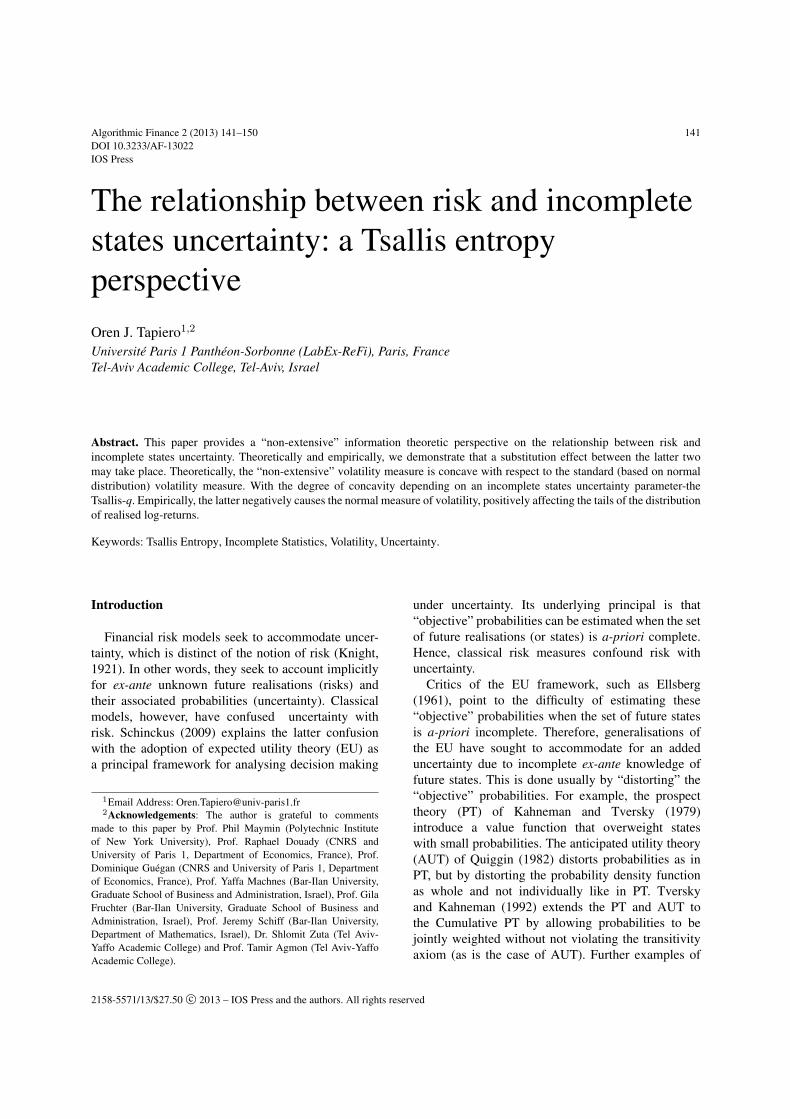
Figure 1 plots equation (4) for several values of qassuming xt is standardised as well as the escort p.d.fused in equation (3).

Using equation (4) and equation (2), a functionalform of uncertainty (Hq [f(xt)]) is obtained. Thisuncertainty is now determined by a “non-extensive”volatility parameter (σq) and a parameter q. Inserting∫ +∞−∞ fq(xt)dxt in equation (2) and taking the limitsq → 1 and q → 3, yields the followings:

limq→1

Hq [f(xt)] = 2 ln(2πσ21e) and

limq→3

Hq [f(xt)] =12

(5)

Interestingly, “non-extensive” uncertainty(Hq[f(xt)]) converges to 1

2 as q → 3 regardless of σq .To explain it, a closer analysis of σq and its relationto the classical measure of standard deviation (σ) isrequired.

1.2. Risk and state incompleteness

Using equation (2) and equation (4) allows also torelate volatility to the associated Lagrange multiplier(β) and to the Tsallis entropy:

σ2q =

1− (q − 1)Hq [f(xt)]β(3− q)

(6)


0.1

0.2

0.3

0.4

0.5

0.1

−5 −4 −3 −2 −1 1 2 3 4 5

q = 1q = 1.6q = 2.5Escort p.d.fp.d.f

0.2

0.3

0.4

0.5

0.6

0.7

Fig. 1. The Tsallis p.d.f. for different values of q (bottom panel) and a comparison between the Tsallis p.d.f. and its escort p.d.f. used inequation (3)

A direct implication of this result is that for q= 1,equation (6) becomes the solution of Boltzmann’sentropy maximisation (i.e: β= 1

σ21

). Therefore, itis possible to assume that β is the same regardlessof whether Tsallis or Boltzmann entropy are beingmaximised. However, for the volatility it is not quitethe case.

Using equation (4) and writing σ1 and σq as“volatilities” corresponding respectively to the solu-tions of maximising Boltzmann’s and Tsallis entropies,a functional form of σq is deduced:

σq = σ2

1+q

1 B(q) (7)

Where:

B(q) =

2π

12−

q2 (q − 1)Γ

(12 + 1

q−1

)(Γ( 1q−1−

12 )

√2

q−1−1

Γ( 1q−1 )

)−q√

(3− q)(q − 1)Γ(

1q−1

)

11+q

(8)

Equation (7), thus, relates the “non-extensive”volatility (σq) to the q parameter and the traditionalnormal measure of volatility (i.e.: standard deviation– σ1). Naturally, σq converges to σ1 as q→ 1.However, taking the limits of σq when q→ 3 yields thefollowing:

limq→3

σq = 0 (9)

Considering the narrative of incomplete statistics,the above result is perhaps surprising as one would

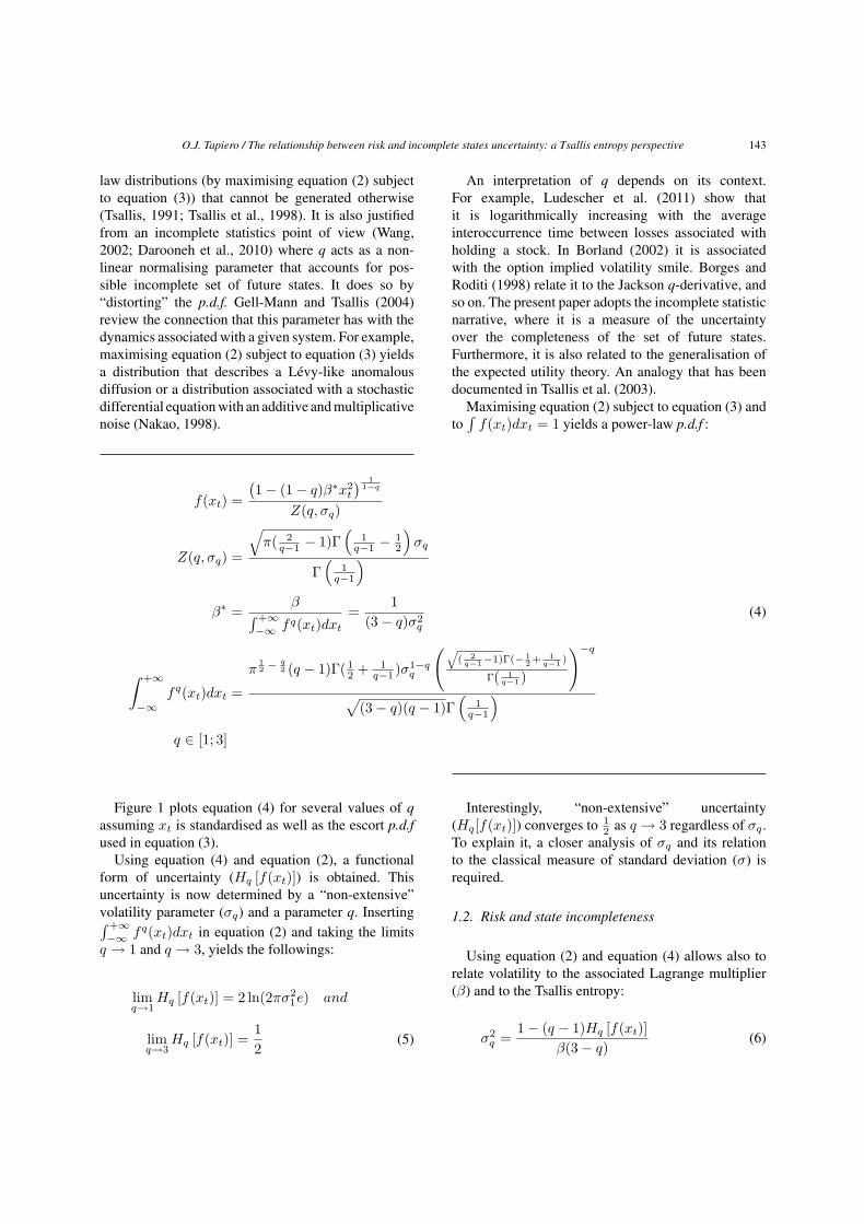
expect σq to be absolutely increasing with q. Never-theless, equation (8) may suggest that from a “non-extensive” perspective, there is a substitution effectthat takes place between σq (measuring risk) and qthat relates to incomplete state uncertainty. This effectis more pronounced when the normal measure ofvolatility and the q parameter are increasing. Figure 2plots equation (7) for given values of q and σ1. Itindicates the concavity of σq with respect to σ at a pre-determined value of q > 1. Some of the empirical im-plications of this relationship are discussed in the nextsection.


q = 1q = 2q = 2.8

0 0.05

0

0.1

0.2

0.3

0.10 0.15 0.20σ

σ q

0.25 0.30 0.35

Fig. 2. This figure plots equation (7) for predetermined values of q (black – q=1, red – q=2 and blue – q=3). For a given q > 1, σq is concavewith respect to the normal measure of volatility σ.

1970 1975 1980 1985 1990Year

1.93

Tsa

llis

-qV

olat

ilit

y

1.94

1.95

0.1

0.2

0.3

1995 2000 2005 2010

σqσ1

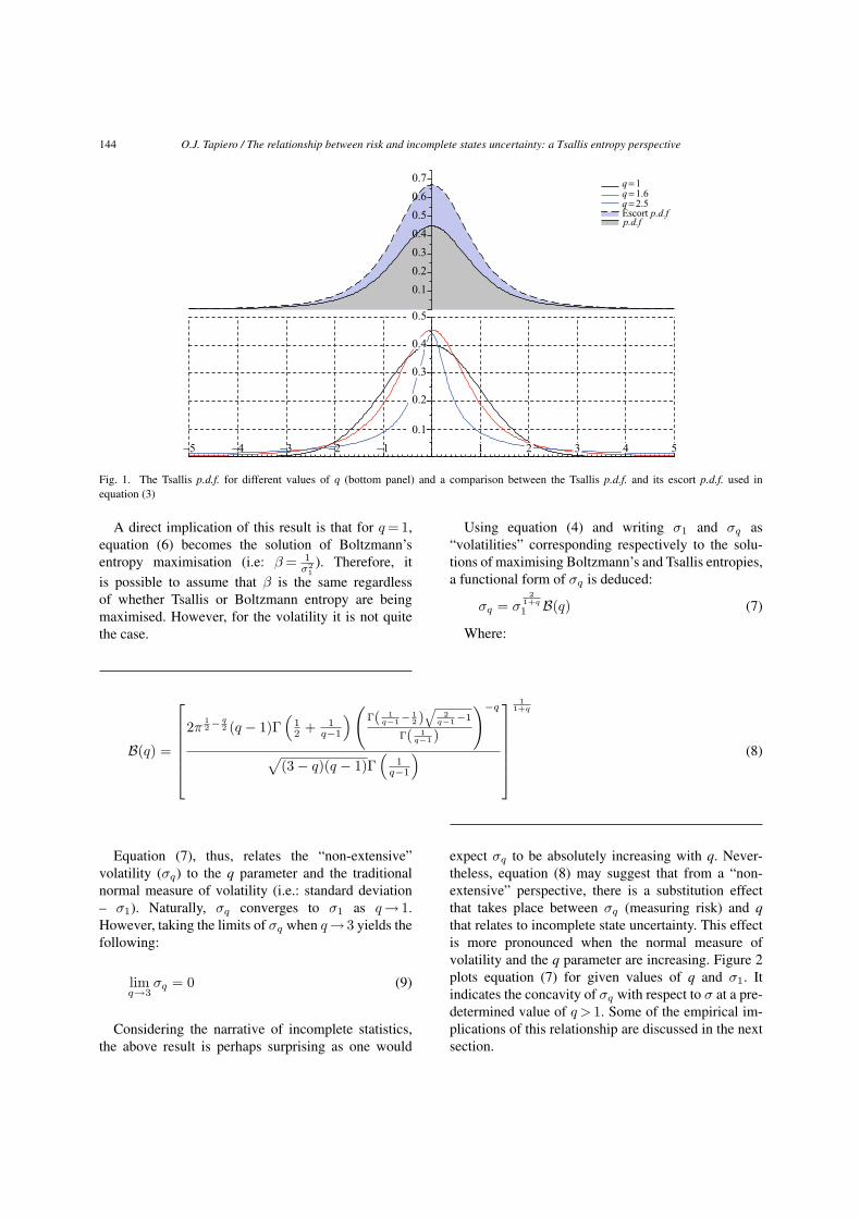
Fig. 3. Top panel indicates the historical (normal) and non-extensive volatility measures (σ1 and σq , respectively). The bottom panel indicatesthe estimated q-parameter.

2. Implications of “non-extensivness” on and riskand uncertainty

Daily closing prices of the S&P-500 and S&P-500implied volatility index (VIX – σV IX ) are downloadedfrom the Yahoo finance2 website. The causality rela-tionship between σ1, σV IX and q are examined. Toestimate q, the log-likelihood function of f(xt|q, σq)(xt being standardised log-returns) is maximised over aselect moving time window. Figure 3 plotsσ1,σq and q,estimated from a moving time window of 5 years. Thecovered period for figure 3 ranges from 1966 to 2012.

2www.finance.yahoo.com

Figure 3 confirms the intuition presented in theprevious section. If the normal volatility measure (σ1)is a measure of risk, relative to the “non-extensive”risk measure (σ1), it underestimate it. Nevertheless,in time frames where tail events occurred (such asOctober 1987 and the 2008 crisis), σ1 relativelyoverstate risk. In such periods, a jump in the value ofq is observed. Figure 3, therefore, may describes wella substitution effect that takes place between (non-extensive) risk and incomplete state uncertainty (q).

The next subsection discusses the possible lead-lag relationship q may have with σ1 and σV IX .The subsection that follows, discuss some of theimplication on portfolio diversification.


2.1. Possible lead-lag relationship with the S&P-500implied volatility index (VIX)

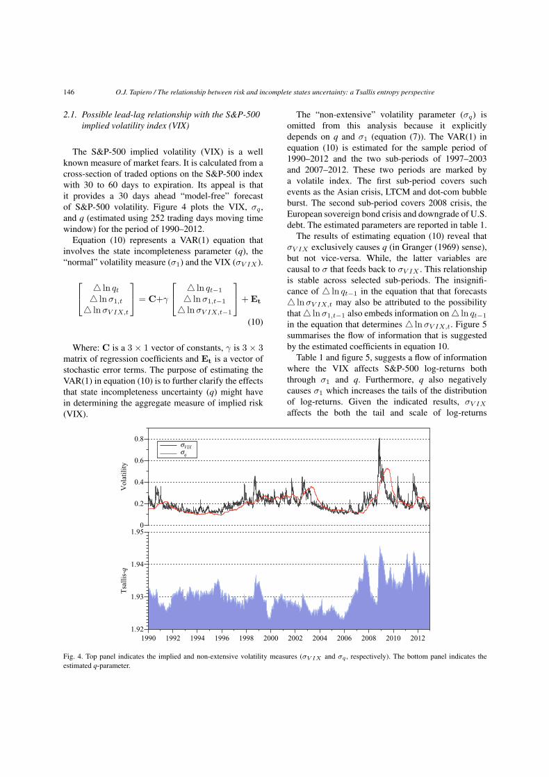
The S&P-500 implied volatility (VIX) is a wellknown measure of market fears. It is calculated from across-section of traded options on the S&P-500 indexwith 30 to 60 days to expiration. Its appeal is thatit provides a 30 days ahead “model-free” forecastof S&P-500 volatility. Figure 4 plots the VIX, σq ,and q (estimated using 252 trading days moving timewindow) for the period of 1990–2012.

Equation (10) represents a VAR(1) equation thatinvolves the state incompleteness parameter (q), the“normal” volatility measure (σ1) and the VIX (σV IX ).

4 ln qt4 lnσ1,t

4 lnσV IX,t

= C+γ

4 ln qt−1

4 lnσ1,t−1

4 lnσV IX,t−1

+ Et

(10)

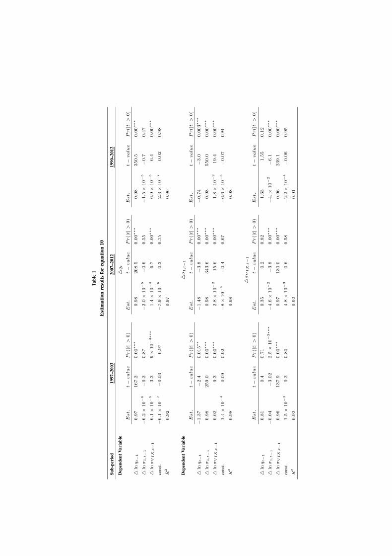
Where: C is a 3 × 1 vector of constants, γ is 3 × 3matrix of regression coefficients and Et is a vector ofstochastic error terms. The purpose of estimating theVAR(1) in equation (10) is to further clarify the effectsthat state incompleteness uncertainty (q) might havein determining the aggregate measure of implied risk(VIX).

The “non-extensive” volatility parameter (σq) isomitted from this analysis because it explicitlydepends on q and σ1 (equation (7)). The VAR(1) inequation (10) is estimated for the sample period of1990–2012 and the two sub-periods of 1997–2003and 2007–2012. These two periods are marked bya volatile index. The first sub-period covers suchevents as the Asian crisis, LTCM and dot-com bubbleburst. The second sub-period covers 2008 crisis, theEuropean sovereign bond crisis and downgrade of U.S.debt. The estimated parameters are reported in table 1.

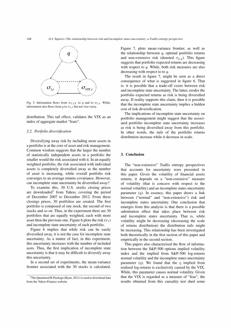
The results of estimating equation (10) reveal thatσV IX exclusively causes q (in Granger (1969) sense),but not vice-versa. While, the latter variables arecausal to σ that feeds back to σV IX . This relationshipis stable across selected sub-periods. The insignifi-cance of 4 ln qt−1 in the equation that that forecasts4 lnσV IX,t may also be attributed to the possibilitythat4 lnσ1,t−1 also embeds information on4 ln qt−1

in the equation that determines 4 lnσV IX,t. Figure 5summarises the flow of information that is suggestedby the estimated coefficients in equation 10.

Table 1 and figure 5, suggests a flow of informationwhere the VIX affects S&P-500 log-returns boththrough σ1 and q. Furthermore, q also negativelycauses σ1 which increases the tails of the distributionof log-returns. Given the indicated results, σV IXaffects the both the tail and scale of log-returns

1990 1992 1994 1996 1998 2000 2002 2004 2006 2008 2010 20121.92

1.93

Tsa

llis

-qV

olat

ilit

y

1.94

1.950

0.2

0.4

0.6

0.8

σq

σVIX

Fig. 4. Top panel indicates the implied and non-extensive volatility measures (σV IX and σq , respectively). The bottom panel indicates theestimated q-parameter.

Tabl

e1

Est

imat

ion

resu

ltsfo

req

uatio

n10

Sub-

peri

od19

97–2

003

2007

–201

219

90–2

012

Dep

ende

ntVa

riab

le4q

t

Est.

t−value

Pr(|t|>

0)

Est.

t−value

Pr(|t|>

0)

Est.

t−value

Pr(|t|>

0)

4lnq

t−

10.9

7167.2

0.0

0∗∗∗

0.9

8208.5

0.0

0∗∗∗

0.9

8350.5

0.0

0∗∗∗

4lnσ1

,t−

1−

6.2×

10−

6−

0.2

0.8

7−

2.0×

10−

5−

0.6

0.5

5−

1.5×

10−

5−

0.7

0.4

7

4lnσ

VI

X,t−

16.1×

10−

53.3

9×

10−

4∗∗∗

1.4×

10−

46.7

0.0

0∗∗∗

6.9×

10−

56.4

0.0

0∗∗∗

cons

t.−

6.1×

10−

7−

0.0

30.9

7−

7.9×

10−

60.3

0.7

52.3×

10−

70.0

20.9

8

R2

0.9

20.9

70.9

6

Dep

ende

ntVa

riab

le4σ1

,t−

1

Est.

t−value

Pr(|t|>

0)

Est.

t−value

Pr(|t|>

0)

Est.

t−value

Pr(|t|>

0)

4lnq

t−

1−

1.3

7−

2.4

0.0

15∗∗

−1.4

8−

3.8

0.0

0∗∗∗

−0.7

4−

3.0

0.0

03∗∗∗

4lnσ1

,t−

10.9

8259.0

0.0

0∗∗∗

0.9

8343.6

0.0

0∗∗∗

0.9

8550.0

0.0

0∗∗∗

4lnσ

VI

X,t−

10.0

29.3

0.0

0∗∗∗

2.8×

10−

215.6

0.0

0∗∗∗

1.8×

10−

219.4

0.0

0∗∗∗

cons

t.1.4×

10−

40.0

90.9

2−

8×

10−

4−

0.4

0.6

7−

6.6×

10−

5−

0.0

70.

94

R2

0.9

80.9

80.9

8

4σ

VI

X,t−

1

Est.

t−value

Pr(|t|>

0)

Est.

t−value

Pr(|t|>

0)

Est.

t−value

Pr(|t|>

0)

4lnq

t−

10.8

10.4

0.7

10.3

50.2

0.8

21.6

31.5

50.1

2

4lnσ1

,t−

1−

0.0

4−

3.0

22.5×

10−

3∗∗∗

−4.6×

10−

2−

3.8

0.0

0∗∗∗

−4.×

10−

2−

6.1

0.0

0∗∗∗

4lnσ

VI

X,t−

10.9

6137.9

0.0

0∗∗∗

0.9

7130.0

0.0

0∗∗∗

0.9

6239.1

0.0

0∗∗∗

cons

t.1.5×

10−

30.2

0.8

04.8×

10−

30.6

0.5

8−

2.2×

10−

4−

0.0

60.9

5

R2

0.9

20.9

20.9

1


Fig. 5. Information flows from σV IX to q and to σ1,t. While,information also flows from q to σ1,t but not vice-versa.

distribution. This tail effect, validates the VIX as anindex of aggregate market “fears”.

2.2. Portfolio diversification

Diversifying away risk by including more assets ina portfolio is at the core of asset and risk management.Common wisdom suggests that the larger the numberof statistically independent assets in a portfolio thesmaller would the risk associated with it. In an equallyweighted portfolio, the risk associated with individualassets is completely diversified away as the numberof asset is increasing, while overall portfolio riskconverges to an average returns covariance. However,can incomplete state uncertainty be diversified away?

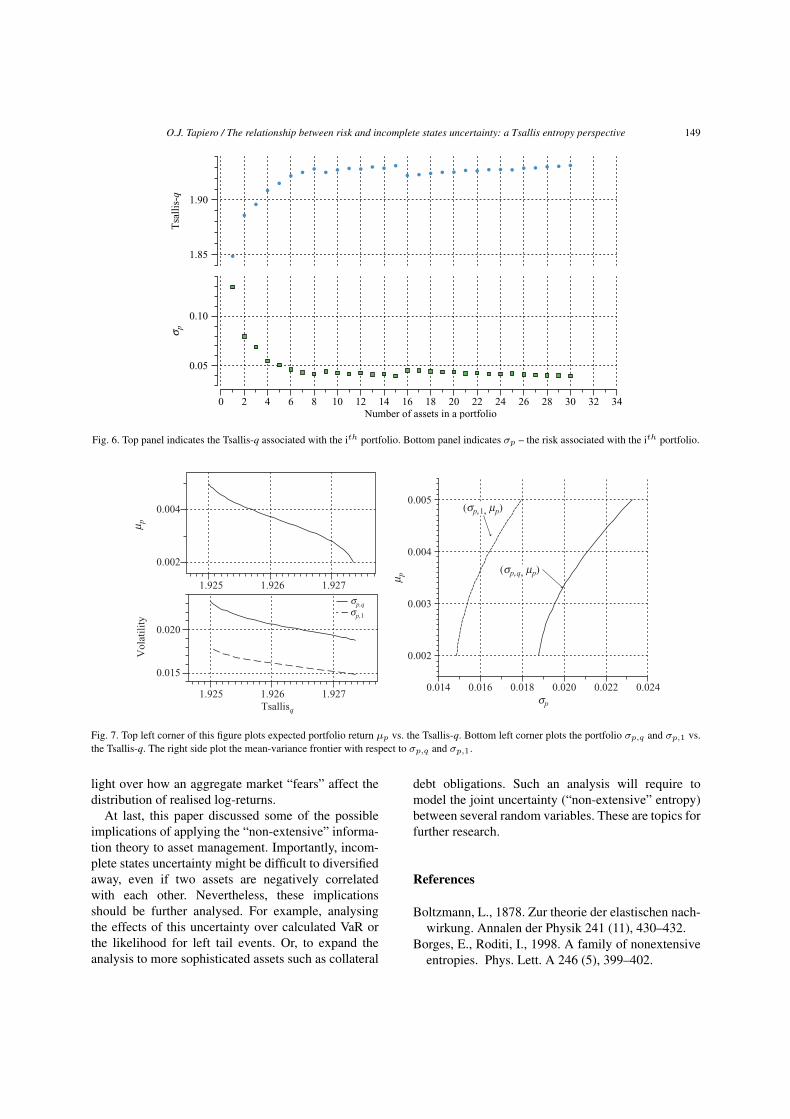
To examine this, 30 U.S. stocks closing pricesare downloaded3 from Yahoo, covering the periodof December 2007 to December 2012. From theseclosings prices, 30 portfolios are created. The firstportfolio is composed of one stock, the second of twostocks and so on. Thus, in the experiment there are 30portfolios that are equally weighted, each with moreasset then the previous one. Figure 6 plots the risk (σ1)and incomplete state uncertainty of each portfolio.

Figure 6 implies that while risk can be easilydiversified away, it is not the case for incomplete stateuncertainty. As a matter of fact, in this experiment,this uncertainty increases with the number of includedassts. Thus, the first implication of incomplete stateuncertainty is that it may be difficult to diversify awaythis uncertainty.

In a second set of experiments, the mean-variancefrontier associated with the 30 stocks is calculated.

3The Quantmod R-Package (Ryan, 2011) is used to download datafrom the Yahoo-Finance website

Figure 7, plots mean-variance frontier, as well asthe relationship between q, optimal portfolio returnsand non-extensive risk (denoted σp,q). This figuresuggests that portfolio expected returns are decreasingwith respect to q. While, both risk measures are alsodecreasing with respect to to q.

The result in figure 7, might be seen as a directconsequence of what is suggested in figure 6. Thatis: it is possible that a trade-off exists between riskand incomplete state uncertainty. The latter, erodes theportfolio expected returns as risk is being diversifiedaway. If reality supports this claim, then it is possiblethat the incomplete state uncertainty implies a hiddencost of risk diversification.

The implications of incomplete state uncertainty onportfolio management might suggest that the associ-ated portfolio incomplete state uncertainty increasesas risk is being diversified away from this portfolio.In other words, the tails of the portfolio returnsdistribution increase while it decrease in scale.

3. Conclusion

The “non-extensive” Tsallis entropy perspectivesthat accounts for uncertainty were presented inthis paper. Given the volatility of financial assetsreturns, it depends on a “non-extensive” measureof volatility (that is concave with respect to thenormal volatility) and an incomplete states uncertaintyparameter (q). In essence, this paper draws a linkbetween (“normal” and “non-extensive”) risk andincomplete states uncertainty. One conclusion thatemerges from this analysis is that there is a possiblesubstitution effect that takes place between riskand incomplete states uncertainty. That is, whilevolatility might be decreasing (decreasing the scaleof returns distribution) the distribution tails mightbe increasing. This relationship has been investigatedboth theoretically in the first section of this paper andempirically in the second section.

This papers also characterised the flow of informa-tion between the S&P-500 options implied volatilityindex and the implied from S&P-500 log-returnsnormal volatility and the incomplete states uncertaintyparameter (q). We found that the q implied fromrealised log-returns is exclusively caused by the VIX.While, this parameter causes normal volatility. Giventhat the VIX is regarded as a measure of “fear”, theresults obtained from this causality test shed some


0 2 4 6 8 10 12 14 16 18Number of assets in a portfolio

20 22 24 26 28 30 32 34

0.05

0.10

σ pT

sall

is-q

1.85

1.90

Fig. 6. Top panel indicates the Tsallis-q associated with the ith portfolio. Bottom panel indicates σp – the risk associated with the ith portfolio.

0.0141.925 1.926 1.927

1.925 1.926 1.927

0.002

0.003

0.015

0.020

0.002

0.004

0.004

0.005

0.016 0.018 0.020 0.022 0.024σp

σp,qσp,1

(σp,1, μp)

(σp,q, μp)

μ p

μ p

Tsallisq

Vol

atil

ity

Fig. 7. Top left corner of this figure plots expected portfolio return µp vs. the Tsallis-q. Bottom left corner plots the portfolio σp,q and σp,1 vs.the Tsallis-q. The right side plot the mean-variance frontier with respect to σp,q and σp,1.

light over how an aggregate market “fears” affect thedistribution of realised log-returns.

At last, this paper discussed some of the possibleimplications of applying the “non-extensive” informa-tion theory to asset management. Importantly, incom-plete states uncertainty might be difficult to diversifiedaway, even if two assets are negatively correlatedwith each other. Nevertheless, these implicationsshould be further analysed. For example, analysingthe effects of this uncertainty over calculated VaR orthe likelihood for left tail events. Or, to expand theanalysis to more sophisticated assets such as collateral

debt obligations. Such an analysis will require tomodel the joint uncertainty (“non-extensive” entropy)between several random variables. These are topics forfurther research.

References

Boltzmann, L., 1878. Zur theorie der elastischen nach-wirkung. Annalen der Physik 241 (11), 430–432.

Borges, E., Roditi, I., 1998. A family of nonextensiveentropies. Phys. Lett. A 246 (5), 399–402.


Borland, L., 2002. Option pricing formulas based ona non-gaussian stock price model. Phys. Rev. Lett.89 (9), 98701.

Borland, L., 2005. Long-range memory and nonexten-sivity in financial markets. Europhys. News 36 (6),228–231.

Chew, S., MacCrimmon, K., 1979. Alpha-Nu ChoiceTheory:AGeneralizationofExpectedUtilityTheory.The University of British Columbia, Canada, BC.

Darooneh, A., Naeimi, G., Mehri, A., Sadeghi, P.,2010. Tsallis entropy, escort probability and theincomplete information theory. Entropy 12 (12),2497–2503.

Ellsberg, D., 1961. Risk, ambiguity, and the savageaxioms. Q. J. Econ. 75 (4), 643–669.

Gell-Mann, M., Tsallis, C., 2004. NonextensiveEntropy: Interdisciplinary Applications. OxfordUniversity Press, USA.

Granger, C., 1969. Investigating causal relations byeconometric models and cross-spectral methods.Econometrica: J. Economet. Soc. 37, 424–438.

Gul, F., 1991. A theory of disappointment aversion.Econometrica: J. Economet. Soc. 59, 667–686.

Jaynes, E., 1957. Information theory and statisticalmechanics. II. Phys. Rev. 108 (2), 171.

Kahneman, D., Tversky, A., 1979. Prospect theory:An analysis of decision under risk. Econometrica: J.Economet. Soc. 47, 263–291.

Karmarkar, U., 1978. Subjectively weighted utility: Adescriptive extension of the expected utility model.Organ. Behav. Hum. Perform. 21 (1), 61–72.

Knight, F., 1921. Risk, Uncertainty and Profit. Reprintof Scarce Texts in Economic and Political Science 16.Signalmen Publishing.

Langlois, R., Cosgel, M., 1993. Frank knight on risk,uncertainty, and the firm: A new interpretation.Econ. Inq. 31 (3), 456–465.

LeRoy, S., Singell, L., 1987. Knight on risk anduncertainty. J. Polit. Econ. 95 (2), 394–406.

Ludescher, J., Tsallis, C., Bunde, A., 2011. Universalbehaviour of interoccurrence times between lossesin financial markets: An analytical description. EPL(Europhys. Lett.) 95 (6), 68002.

Nakao, H., 1998. Asymptotic power law of momentsin a random multiplicative process with weakadditive noise. Phys. Rev. E 58 (2), 1591.

Quiggin, J., 1982. A theory of anticipated utility. J.Econ. Behaviour Organ. 3 (4), 323–343.

Ryan, J., 2011. quantmod: Quantitative financialmodelling framework. R package version 0.3-17.

Schinckus, C., 2009. Economic uncertainty and econo-physics. Physica A: Stat. Mech. Appl. 388 (20),4415–4423.

Shannon, C., 1948. Tech. 27 (1948) 379; bell syst.Tech 27, 623.

Tsallis, C., 1988. Possible generalization of boltzmann-gibbs statistics. J. Stat. Phys. 52 (1), 479–487.

Tsallis, C., 1991. Enf curado and c. tsallis. J. Phys. A24, L69.

Tsallis,C.,Anteneodo,C.,Borland,L.,Osorio,R.,2003.Nonextensive statistical mechanics and economics.Physica A: Stat. Mech. Appl. 324 (1), 89–100.

Tsallis, C., Mendes, R., Plastino, A., 1998. Therole of constraints within generalized nonextensivestatistics. Physica A: Stat. Mech. Appl. 261 (3),534–554.

Tversky, A., Kahneman, D., 1992. Advances in pros-pect theory: Cumulative representation of uncer-tainty. J. Risk. Uncertain. 5 (4), 297–323.

Wang, Q., 2002. Nonextensive statistics and incom-plete information. Eur. Phys. J. B-Condensed Matterand Complex Systems 26 (3), 357–368.

Whaley, R., 2000. The investor fear gauge. J. PortfolioManage. 26 (3), 12–17.

Documents

The relationship between risk and incomplete states uncertainty: a Tsallis entropy perspective