The Spin-Echo System Reconsidered∗

D. A. LavisDepartment of Mathematics

King’s College, Strand, London WC2R 2LS, U. K.Email:David.Lavis@kcl.ac.uk

Abstract

Simple models have played an important role in the discussion of founda-tional issues in statistical mechanics. Among them the spin–echo systemis of particular interest since it can be realized experimentally. This hasled to inferences being drawn about approaches to the foundations of sta-tistical mechanics, particularly with respect to the use of coarse-graining.We examine these claims with the help of computer simulations.

1 Introduction

Kinetic equations are very useful in statistical mechanics but they are, in general,approximations to the behaviour of the underlying systems. Therefore, anyconclusions which can be drawn from them are of limited significance for theresolution of foundational issues. What are needed are ‘exact’ results, or atleast situations in which numerical errors do not affect qualitative behaviour.This is a severe restriction; most interesting problems in statistical mechanicsconcern cooperative systems and, even at equilibrium (see e.g. Baxter, 1982)there are few of these which can be solved exactly. So, of necessity, usefulexamples are of assemblies of non-interacting microsystems and the literaturecontains discussions of many ‘toy models’ of this kind, some stochastic and somedeterministic. Simulations for a number of these are available in Lavis (2003);here we confine our attention to an assembly of magnetic dipoles precessing in afield. We shall investigate the time-evolution of the Boltzmann entropy, the fine-grained and coarse-grained versions of the Gibbs entropy and the magnetization.We reverse the dynamic evolution at an instant of time and demonstrate thatthe system returns to a state equivalent to that at the initial time. This is thespin–echo effect.

1.1 Forms of Entropy

Consider a system, which at time t has a microstate given by the vector x(t) inthe phase-space Γ. Some autonomous dynamics x → φt x, (t ≥ 0) determines aflow in Γ and the set of points x(t) = φtx(0), parameterized by t ≥ 0, gives atrajectory. The set of mappings φtt≥0 is a semi-group. The system is reversibleif there exists a self-inverse operator I on the points of Γ, such that φtx = x′

∗Published (with some typing errors) in Foundations of Physics, 34, 669–688 (2004).

1

implies that φtI x′ = I x. Then φ−t = (φt)−1 = IφtI and the set φt witht ∈ R or Z is a group.

1.1.1 The Boltzmann Entropy

Macrostates (observable states) are defined by a set Ξ of macroscopic variables.1

Let the set of macrostates be µΞ. They are so defined that every x ∈ Γ isin exactly one macrostate denoted by µ(x) and the mapping x → µ(x) ismany-one. Every macrostate µ is associated with its ‘volume’ VΞ(µ) in Γ.2 Wethus have the map x → µ(x) → VΞ(x) ≡ VΞ(µ(x)) from Γ to R

+ or N. TheBoltzmann entropy is defined by

SB(x) = kB ln[VΞ(x)]. (1)

This is a phase function depending on the choice of macroscopic variables Ξ.Suppose the system consists of N identical microsystems.3 Then ΓN is the

direct product of N copies of Γ1, the phase-space of one microsystem. Let x(i)(t)be the phase vector of the i-th microsystem moving in its Γ1. Now divide Γ1

into a enumerable set of cells γk of equal volume ν such that every point inΓ1 belongs to exactly one γk. The macroscopic variables Ξ are taken to be theset Nk of coarse-graining variables, where Nk is the number of microsystemswith phase-points in γk. Then a macrostate is the part of ΓN corresponding toa fixed set of values of Nk and

VNk(x) = Ω(Nk(x))νN , Ω(Nk) =N !∏

k(Nk)!, (2)

SB(x) = kB ln[Ω(Nk(x))] + kBN ln(ν). (3)

This formula is valid irrespective of whether the microsystems are interacting.However, if they are, then constraints will apply to the possible values of Nk.4

1.1.2 The Gibbs Entropy

The fine-grained Gibbs entropy5 is given by the functional

SFGG[ρN(t)] = −kB

∫ΓN

ρN(x; t) lnρN(x; t)dΓN . (4)

of the fine-grained probability density function ρN(x; t) on ΓN . For a measure-preserving system for which ρN(x; t) satisfies Liouville’s equation SFGG[ρN(t)]remains constant with time, as we shall demonstrate explicitly for the spinsystem in Sec. 2. The resolution to this problem suggested by Gibbs (1902, p.148) (see also Ehrenfest and Ehrenfest-Afanassjewa, 1912) is to coarse-grain the

1These may include some thermodynamic variables (volume, number of particles etc.) butthey will also include other variables, specifying, for example, the number of particles in a setof subvolumes. Ridderbos (2002) denotes these by the collective name of supra-thermodynamicvariables.

2The term ‘volume’ being taken to mean some appropriate measure on Γ.3In indication of which we denote the phase-space by ΓN .4Representing, for example, the condition that the phase point of the whole system must

lie on an energy hypersurface in ΓN .5The ‘fine-grained’ qualification to the Gibbs entropy and probability density function is

a convenient distinction from the coarse-grained versions defined below.

2

phase-space ΓN , in the manner in which macrostates have been obtained in theBoltzmann approach. We first note that for a system of identical non-interactingmicrosystems the probability density function factorizes into a product of single-microsystem densities.

ρN(x; t) =N∏

i=1

ρ1(x(i); t). (5)

Then

SFGG[ρN(t)] = −kBN

∫Γ1

ρ1(x; t) lnρ1(x; t)dΓ1. (6)

Using the cells γk defined in Sec. 1.1.1 we define the coarse-grained probabilitydensity by

ρ1(k; t) =∫

γk

ρ1(x; t)dΓ1 (7)

and the coarse-grained Gibbs entropy by

SCGG[ρN(t)] = −kBN∑

k

ρ1(k; t) lnρ1(k; t) + kBN ln(ν). (8)

The second term in (8) is required for consistency with the fine-grained entropyin the case where the fine-grained density is uniform (with possibly differentvalues) over each of the cells. Then, from (7), ρ1(k; t) = νρ1(xk; t), where xk isany point in γk and substituting into (6) gives (8).6

If we begin with any fine-grained density ρN(x; t) and calculate SFGG[ρN(t)],and then apply coarse-graining and calculate SCGG[ρN(t)],

SFGG[ρN(t)] ≤ SCGG[ρN(t)], (9)

with equality only if the fine-grained density is uniform over the cells of thecoarse-graining. Now we can conceive of two possible ways of tracing the evo-lution of entropy in the Gibbs coarse-grained picture.

(i) We could begin with some fine-grained density giving entropy SFGG[ρN(0)]at t = 0 and watch its evolution as time increases. If at time t′ ≥ 0 wecoarse-grain, then

SFGG[ρN(0)] = SFGG[ρN(t′)] ≤ SCGG[ρN(t′)]. (10)

However if we coarse-grain at two instants 0 ≤ t′ < t′′ it is not necessarilythe case that

SCGG[ρN(t′)] ≤ SCGG[ρN(t′′)]. (11)

The coarse-grained entropy will not necessarily show monotonic increase.However, the graph of the coarse-grained entropy will not depend on theinstants at which coarse-graining is applied.

6Alternatively the final term in (8) could be absorbed if the formula were written in the formof an integral (rather than summation) over the piecewise constant coarse-grained density.

3

(ii) If, instead of the strategy adopted in (i) we coarse-grain at t′ then followthe evolution of the coarse-grained density and then re-coarse-grain at thelater time t′′, (11) will hold. Course-grained entropy will show monotonicincrease. However, the graph of entropy against time will be affected bythe instances at which coarse-graining is applied.

From (2)–(3), using Stirling’s formula for large N ,7

SB(x) −kBN∑

k

Nk(x)N

ln(

Nk(x)N

)+ kBN ln(ν). (12)

The relationship between (8) and (12) is now easy to see. If on the one handa very large assembly of microsystems is taken with initial density in Γ1 ofNρ1(x; 0) then Nk(t)/N , the proportion of the assembly in cell γk at time t isρ1(k; t) given by (7) and (12) is asymptotically equivalent to (8). Conversely,if in the Gibbs formulation the initial density function is chosen to be a set ofN suitably-weighted Dirac delta functions, we recover (12). In summary, weexpect the Boltzmann entropy in the limit of large N and close to the uniformdistribution to converge to the coarse-grained Gibbs entropy.

2 The Model

Consider the simple model in which a magnetic dipole of moment m is fixed atits centre but is free to rotate in the presence of a constant magnetic field B.The equation of motion of the dipole will be

m(t) = g m(t) ∧ B, (13)

where g is the gyromagnetic ratio. Released from rest the dipole will precess ata constant angle to B. In particular, if m is located at the origin of a cartesiancoordinate system with B in the direction of the negative z-axis and if initiallym lies in the x− y plane, its subsequent motion remains in the x− y plane andis given by

m(t) = (m cos(θ(t)), m sin(θ(t))), (14)

where

θ(t) = φt θ(0) = F2π(θ(0) + ωt), ω = B g, (15)

and8

Fα(x) = α × Non-Integer Part(x

α

). (16)

Suppose that at some time t = τ the magnetic field B is turned off and a fieldB′, in the direction of the x–axis is turned on for a time t′ = π/B′g. The effect ofthis will be to rotate the dipole through an angle π about the x-axis, translatingits position from θ(τ) = F2π(θ(0) + ωτ) to θ′(τ) = 2π − F2π(θ(0) + ωτ) =

7In fact the approximation is close only when not only N , but all the Nk are large. Thismeans that it is good only for large N and a distribution of microsystems close to the uniformdistribution over the cells.

8Where, of course, Fα(x ± Fα(y)) = Fα(x ± y), for all real x and y and positive α.

4

F2π(2π − θ(0) − ωτ); a reflection in the x-axis. We denote this self-inversereflection operator by R; that is R(θ, ω) = (2π − θ, ω). With reflection appliedat t = τ

θ(2τ) = F2π(θ′(τ) + ωτ) = 2π − θ(0). (17)

This reflectional return or echo-effect is what gives the system its name. Themodel is also reversible with I(θ, ω) = (θ,−ω). Then

θ(2τ) = φ−τθ(τ) = F2π(θ(τ) − ωτ) = θ(0). (18)

So the system has two mechanisms for making it ‘retrace its steps’. However,this is not so strange. It would be true for any system with periodic boundaryconditions; and a similar effect occurs when a particle is in one-dimensionalmotion at constant speed v confined between elastic walls at x = 0 and x = L.Then we can ‘unfold’ right-to-left motions of the particle into the region [L, 2L].The model is now equivalent to the dipole motion with π replaced by L. Theecho transformation x → 2L − x at t = τ is now exactly the same as reversingthe direction of the velocity, with x(2τ) = x(0) and x(2τ) = −x(0). However,there is a second possible transformation x → L − x. Now x(2τ) = L − x(0)and x(2τ) = x(0). For an assembly of particles this fulfills the purposes of theecho transformation just as well.9

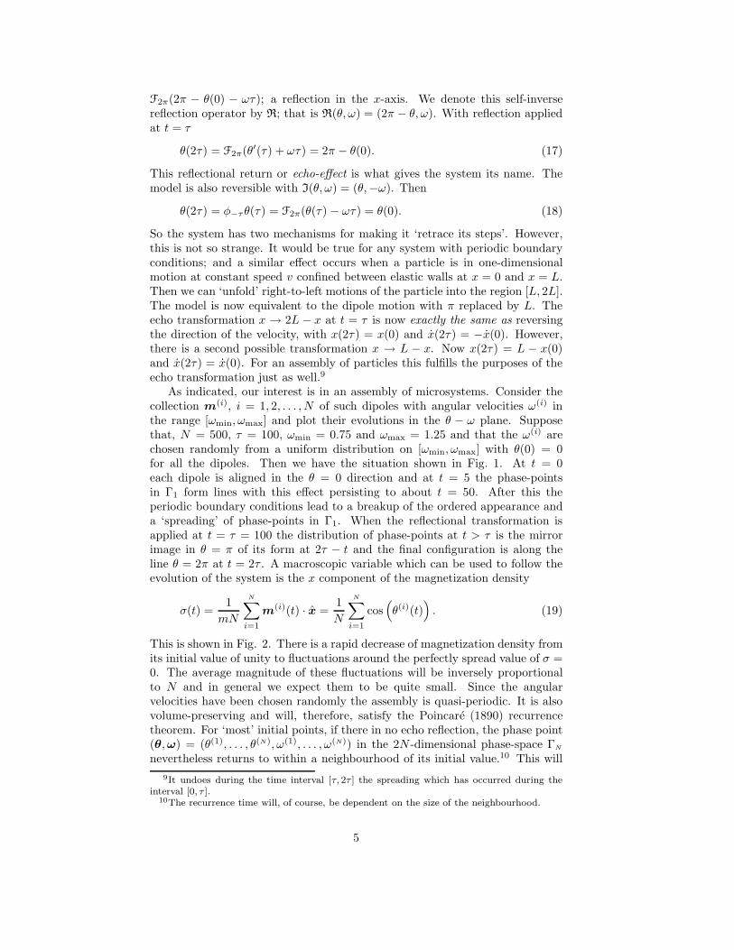
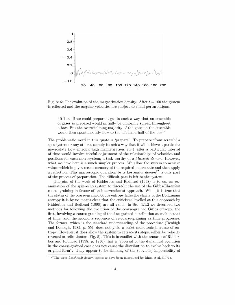
As indicated, our interest is in an assembly of microsystems. Consider thecollection m(i), i = 1, 2, . . . , N of such dipoles with angular velocities ω(i) inthe range [ωmin, ωmax] and plot their evolutions in the θ − ω plane. Supposethat, N = 500, τ = 100, ωmin = 0.75 and ωmax = 1.25 and that the ω(i) arechosen randomly from a uniform distribution on [ωmin, ωmax] with θ(0) = 0for all the dipoles. Then we have the situation shown in Fig. 1. At t = 0each dipole is aligned in the θ = 0 direction and at t = 5 the phase-pointsin Γ1 form lines with this effect persisting to about t = 50. After this theperiodic boundary conditions lead to a breakup of the ordered appearance anda ‘spreading’ of phase-points in Γ1. When the reflectional transformation isapplied at t = τ = 100 the distribution of phase-points at t > τ is the mirrorimage in θ = π of its form at 2τ − t and the final configuration is along theline θ = 2π at t = 2τ . A macroscopic variable which can be used to follow theevolution of the system is the x component of the magnetization density

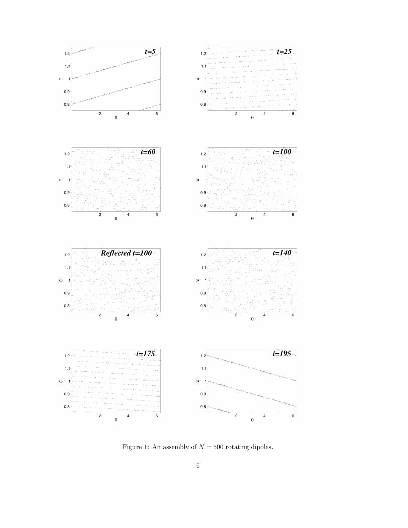
σ(t) =1

mN

N∑i=1

m(i)(t) · x =1N

N∑i=1

cos(θ(i)(t)

). (19)

This is shown in Fig. 2. There is a rapid decrease of magnetization density fromits initial value of unity to fluctuations around the perfectly spread value of σ =0. The average magnitude of these fluctuations will be inversely proportionalto N and in general we expect them to be quite small. Since the angularvelocities have been chosen randomly the assembly is quasi-periodic. It is alsovolume-preserving and will, therefore, satisfy the Poincare (1890) recurrencetheorem. For ‘most’ initial points, if there in no echo reflection, the phase point(θ, ω) = (θ(1), . . . , θ(N), ω(1), . . . , ω(N)) in the 2N -dimensional phase-space ΓN

nevertheless returns to within a neighbourhood of its initial value.10 This will9It undoes during the time interval [τ, 2τ ] the spreading which has occurred during the

interval [0, τ ].10The recurrence time will, of course, be dependent on the size of the neighbourhood.

5

t=5

0.8

0.9

1

1.1

1.2

ω

2 4 6θ

t=25

0.8

0.9

1

1.1

1.2

ω

2 4 6θ

t=60

0.8

0.9

1

1.1

1.2

ω

2 4 6θ

t=100

0.8

0.9

1

1.1

1.2

ω

2 4 6θ

Reflected t=100

0.8

0.9

1

1.1

1.2

ω

2 4 6θ

t=140

0.8

0.9

1

1.1

1.2

ω

2 4 6θ

t=175

0.8

0.9

1

1.1

1.2

ω

2 4 6θ

t=195

0.8

0.9

1

1.1

1.2

ω

2 4 6θ

Figure 1: An assembly of N = 500 rotating dipoles.

6

σ

t

–0.2

0

0.2

0.4

0.6

0.8

1

20 40 60 80 100 120 140 160 180 200

Figure 2: The evolution of the magnetization density. After t = τ = 100 thebroken line gives the echo.

lead to a large fluctuation in magnetization density. Of course, if the initialangular velocities are chosen to be commensurate, the system will be periodicand will return exactly to its initial point with σ = 1.

There would be nothing particularly special about this model, if it were notfor the fact that it has been realized experimentally. Hahn (1950) (see also Hahn,1953; Rhim et al., 1971; Brewer and Hahn, 1984) applied a magnetic field tovarious liquids whose molecules contain hydrogen atoms. By manipulating thecomponents of the magnetic field he was able to start with the dipole momentsof the proton spins in the x–direction, make them precess around the z–axis andthen reflect the directions of the dipoles in the x–axis to achieve the echo effectwith the dipoles returning to their initial alignment.11 This system has arousedsome interest in relation to questions of reversibility in statistical mechanics(Blatt, 1959; Mayer and Mayer, 1977; Denbigh and Denbigh, 1985; Ridderbosand Redhead, 1998; Ridderbos, 2002). This will be discussed in Sec. 3. Here weshall simply present the results of our calculations.

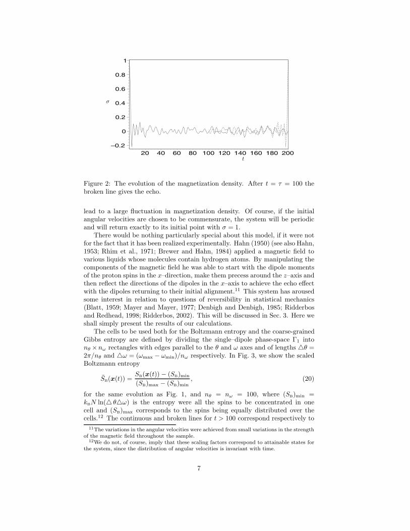
The cells to be used both for the Boltzmann entropy and the coarse-grainedGibbs entropy are defined by dividing the single–dipole phase-space Γ1 intonθ ×nω rectangles with edges parallel to the θ and ω axes and of lengths θ =2π/nθ and ω = (ωmax − ωmin)/nω respectively. In Fig. 3, we show the scaledBoltzmann entropy

SB(x(t)) =SB(x(t)) − (SB)min

(SB)max − (SB)min, (20)

for the same evolution as Fig. 1, and nθ = nω = 100, where (SB)min =kBN ln( θω) is the entropy were all the spins to be concentrated in onecell and (SB)max corresponds to the spins being equally distributed over thecells.12 The continuous and broken lines for t > 100 correspond respectively to

11The variations in the angular velocities were achieved from small variations in the strengthof the magnetic field throughout the sample.

12We do not, of course, imply that these scaling factors correspond to attainable states forthe system, since the distribution of angular velocities is invariant with time.

7

SB

t

0.8

0.85

0.9

0.95

1

0 20 40 60 80 100 120 140 160 180 200

Figure 3: The evolution of the Boltzmann entropy of the dipole assembly. Aftert = τ = 100 the broken line gives the echo.

the evolutions without and with the echo-effect.We now calculate the fine-grained Gibbs entropy. Suppose that the initial

probability density function is concentrated and uniform over the rectangle ω ∈[ωmin, ωmax], θ ∈ [0, θ0], (θ0 < 2π). Then

ρ1(θ, ω; 0) =H(θ) − H(θ − θ0)θ0(ωmax − ωmin)

, (21)

where H(θ) is the Heaviside unit function, and

ρ1(θ, ω; t) =

⎧⎪⎪⎪⎪⎪⎪⎪⎪⎨⎪⎪⎪⎪⎪⎪⎪⎪⎩

H(θ − F2π(ωt)) − H(θ − F2π(θ0 + ωt))θ0(ωmax − ωmin)

,

F2π(ωt) < F2π(θ0 + ωt),

H(θ − F2π(ωt)) − H(θ − F2π(θ0 + ωt)) + H(θ) − H(θ − 2π)θ0(ωmax − ωmin)

,

F2π(θ0 + ωt) < F2π(ωt).

(22)

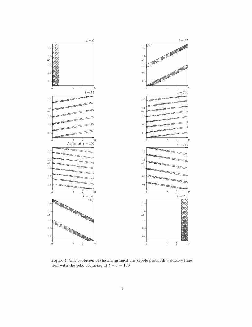
If the echo transformation θ → 2π − θ is applied at the time τ the one-spinprobability density function for t > τ is given, in terms of (22) by ρ1(2π −θ, ω; 2τ − t). The evolution of this fine-grained probability density function,with τ = 100, is shown in Fig. 4. Over the time interval [0, τ ] the cross-hatchedregion spreads itself in ever-thinner striations over Γ1 and this process wouldcontinue if the echo transformation were not applied.13 The effect of the echo-transformation is as in Fig. 1; it produces a configuration at t > τ which is thereflection in θ = π of the configuration at 2τ − t. Substituting from (22) into(6) gives

SFGG[ρN(t)] = kBN lnθ0(ωmax − ωmin). (23)13However, we have to be a little cautious about this since we are considering a collection

of non-interacting dipoles. For each dipole the second equation of motion to pair with (15)is ω(t) = ω(0). Motion is horizontal in Γ1 and, unlike for example a gas of particles mov-ing according to the baker’s transformation (Lavis, 2003), and contrary to the assertion byRidderbos and Redhead (1998, p. 1248) the system is mixing in Γ1 only in a limited sense.

8

ω

θ

t = 0

0.8

0.9

1.0

1.1

1.2

0 π 2π

ω

θ

t = 25

0.8

0.9

1.0

1.1

1.2

0 π 2π

ω

θ

t = 75

0.8

0.9

1.0

1.1

1.2

0 π 2π

ω

θ

t = 100

0.8

0.9

1.0

1.1

1.2

0 π 2π

ω

θ

Reflected t = 100

0.8

0.9

1.0

1.1

1.2

0 π 2π

ω

θ

t = 125

0.8

0.9

1.0

1.1

1.2

0 π 2π

ω

θ

t = 175

0.8

0.9

1.0

1.1

1.2

0 π 2π

ω

θ

t = 200

0.8

0.9

1.0

1.1

1.2

0 π 2π

Figure 4: The evolution of the fine-grained one-dipole probability density func-tion with the echo occurring at t = τ = 100.

9

SCGG

t

0.4

0.6

0.8

1

0 50 100 150 200

Figure 5: The evolution of the coarse-grained Gibbs entropy of the dipole as-sembly. After t = τ = 100 the broken line corresponds to the echo.

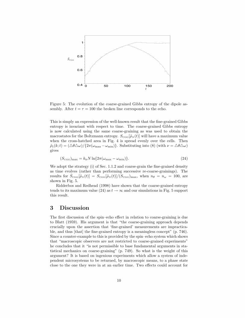
This is simply an expression of the well-known result that the fine-grained Gibbsentropy is invariant with respect to time. The coarse-grained Gibbs entropyis now calculated using the same coarse-graining as was used to obtain themacrostates for the Boltzmann entropy. SCGG[ρN(t)] will have a maximum valuewhen the cross-hatched area in Fig. 4 is spread evenly over the cells. Thenρ1(k; t) = (θω)/2π(ωmax−ωmin). Substituting into (8) (with ν = θω)gives

(SCGG)max = kBN ln2π(ωmax − ωmin). (24)

We adopt the strategy (i) of Sec. 1.1.2 and coarse-grain the fine-grained densityas time evolves (rather than performing successive re-coarse-grainings). Theresults for SCGG[ρN(t)] = SCGG[ρN(t)]/(SCGG)max, when nθ = nω = 100, areshown in Fig. 5.

Ridderbos and Redhead (1998) have shown that the coarse-grained entropytends to its maximum value (24) as t → ∞ and our simulations in Fig. 5 supportthis result.

3 Discussion

The first discussion of the spin–echo effect in relation to coarse-graining is dueto Blatt (1959). His argument is that “the coarse-graining approach dependscrucially upon the assertion that ‘fine-grained’ measurements are impractica-ble, and thus [that] the fine-grained entropy is a meaningless concept” (p. 746).Since a counter-example to this is provided by the spin–echo system which showsthat “macroscopic observers are not restricted to coarse-grained experiments”he concludes that it “is not permissible to base fundamental arguments in sta-tistical mechanics on coarse-graining” (p. 749). So what is the weight of thisargument? It is based on ingenious experiments which allow a system of inde-pendent microsystems to be returned, by macroscopic means, to a phase stateclose to the one they were in at an earlier time. Two effects could account for

10

‘closeness’ rather than exact return. The first would be be an internal coopera-tive effect, in this case a spin–spin coupling.14 Blatt (1959, p. 750) remarks thatthe decrease in the echo–pulse arising from this is “from [the] present point ofview accidental”. He is content to consider a system of independent microsys-tems, because in any event the inclusion of cooperative effects would not allowan escape from the iron hand of Liouville’s theorem; the fine-grained Gibbsentropy would still be constant. He is interested in the external (spin–lattice)source of the deviation from exact return. This interventionist alternative tocoarse-graining, which is also the position of Ridderbos and Redhead (1998) andRidderbos (2002) will not be discussed here. Rather we return to the originalcontention that the demonstration of a system which can be controlled more-or-less exactly at the microscopic level by macroscopic means is the death-blowfor coarse-graining. Of course, the coarse-graining referred to by Blatt (andalso by Ridderbos and Redhead and Ridderbos) is of the Gibbs–Ehrenfest typeand it is true that Tolman (1938, p. 167) in justifying this argues that “inmaking any actual measurement of the [macroscopic variables] of the system. . . we ordinarily do not achieve the precise knowledge of their values theoret-ically permitted by classical mechanics”. But if this were the main argumentfor coarse-graining of the Gibbs–Erhenfest or Boltzmann kind it would be veryweak. It has always been possible to obtain analytic solutions for assemblies ofnon-interacting microsystems and with the advent of fast computing we can, aswe have here, produce data for assemblies of arbitrary size. The fact that such asystem can be realized experimentally and controlled macroscopically may havebeen of great importance technically, but it is hardly a milestone in foundationaldevelopment. In fact it is not clear that either Gibbs (1902) or Ehrenfest andEhrenfest-Afanassjewa (1912) intended to justify the procedure by an appealto the limitations of measurement. Gibbs (ibid, p. 148) refers to the cells ofthe coarse-graining as being “so small that [the fine-grained probability densityfunction] may in general be regarded as sensibly constant within any one ofthem at the initial moment” and the Ehrenfests (ibid, p. 52) simply observethat the cells must be “small, but finite”. In the case of the Boltzmann entropythe situation is somewhat clearer. The size of the cells defines the ‘macro-scale’as distinct from the ‘micro-scale’ (Lebowitz, 1993). Of course, this demarcationis to some extent arbitrary, but it is equally so for any macroscopic physicaltheory.15 As is pointed out by Grunbaum (1975), Boltzmann’s entropy can beregarded as a measure of homogeneity and in this context the equilibrium statecorresponds simply to the maximum entropy state, which has the most homo-geneity. It is precisely and only here, in defining a measure for homogeneity atequilibrium (Ridderbos, 2002), that the demarcation between the macro- andmicro-scales must be made. And this is unavoidable since no distribution ofdiscrete points over a continuum is uniform on all scales.

We now consider the case made by Denbigh and Denbigh (1985, p. 49–50 and140–143)16 for the assertion that the spin–echo system exemplifies circumstancesthat are “highly exceptional” in reproducing the kind of reversible situation usedby Loschmidt (1876) in his challenge to Boltzmann. The argument hinges ona comparison between a gas expanding in a box and the spin–echo system.

14Similar experiments including dipolar coupling were performed by Rhim et al. (1971).Whilst these are of importance expermentally they do not affect the argument.

15See e.g. the definition of fluid density in Landau and Lifshitz (1959, p. 1).16The same argument is reproduced in Ridderbos and Redhead (1998, p. 1253–1254).

11

This already presents some problems since, as we have shown in Sec. 2, thestates of a particle moving in one dimension between perfectly reflecting barriersare isomorphic to those of a single spin precessing in a field with the spin–echo reflection equivalent to velocity inversion. It follows from this that non-interacting assemblies of each of these are isomorphic.17 A summary of thesituation considered by Denbigh and Denbigh (1985, p. 49–50) is as follows:18

(i) Let A → B be a “macroscopic process” from a thermodynamic state A toa thermodynamic state B.

(ii) Let S(A) and S(B) be “those sets of exactly specified microstates whichare accessible to the gas” in states A and B.

(iii) Let IS(A) and IS(B) be those sets of macrostates obtained from S(A) andS(B) by reversing the velocities.

(iv) If x(0) ∈ S(A) and x(τ) ∈ S(B) then Ix(τ) ∈ IS(B) and φτIx(τ) =Ix(0) ∈ IS(A).

The inference is drawn that, if the system during the evolution x(0) → x(τ)goes from A to B, there is an allowed evolution Ix(τ) → Ix(0), taking thesystem from B to A.19 If thermodynamic entropy increases in one directionit will decrease in the other. This is the heart of Loschmidt’s paradox. In hisreply to Loschmidt, Boltzmann (1877) pointed out that, whereas the trajectoriesfrom the majority of the points in S(A) will yield an increase in entropy in thetime interval [0, τ ], only a small percentage of the points in IS(B) will yieldtrajectories giving a decrease in entropy over [0, τ ]. Denbigh and Denbigh (1985,p. 50) accept the general validity of this argument, but they believe that thespin–echo system where velocity inversion I is replaced by reflection R is aspecial case. They claim (translating into our notation) that “the situation [inthe spin–echo system] is that the set of the type [RS(B)] contains the samenumber of members as the set of type [S(A)]; for every original spin thereis a spin with a reversed velocity of precession”.20 This statement containstwo parts the first contentious and the second obviously true. It is certainlytrue that to every spin state there is another with the velocity of precessionreversed (or the position reflected). A similar statement would be true for anyreversible dynamic system. The distinguishing, although possibly not unique,feature of the spin system is that “these velocities can actually be reversedsimultaneously by applying a magnetic pulse”. But this is a technical featurewhich could always be anticipated for a system of non-interacting microsystems.On the other hand if the first part of the statement (that RS(B) contains the

17It may be that Denbigh and Denbigh are effectively arguing that a two-dimensional gasof particles in a box B = (x, y)|0 ≤ x ≤ L, 0 ≤ y ≤ L where each particle moves at constantspeed in the x-direction without any collisions is itself “highly exceptional”. If so the spin–echosystem is irrelevant, except in so far as it is realized experimentally.

18They begin by referring to a gas of particles in a box where the operation needed to makethe system retrace its steps is velocity reversion.

19There is one benign gap in this argument. It is assumed that the thermodynamic statesfor the reversed process are the same as those for the forward process. This is equivalent tosupposing that, if x ∈ S(A), then Ix ∈ S(A). In other words, IS(A) ≡ S(A), IS(B) ≡ S(B).The truth of these identities, although plausible, will, of course, depend on the meaning (yetto be discussed) of ‘accessible’.

20See also Ridderbos and Redhead (1998, p. 1254) for a similar assertion.

12

same number of members as S(A)) were true this would be in conflict withBoltzmann’s answer to Loschmidt and it would be necessary to give an argumentwhy this does not contradict the second law.21 The problem with understandingthis argument is in interpreting the term ‘accessible’.22 Let us suppose that it isto be interpreted as all those microstates compatible with a given value for thex component of the magnetization mNσ(t).23 If initially σ(0) = 1, then all thespins must be aligned with the x-axis; θ(0) =

(θ(1)(0), . . . , θ(N)(0)

)= 0 and

the microstates S(A) accessibly to this macrostate A correspond to all possiblevalues of ω = (ω(1), . . . , ω(N)). Now we have to define the final state B at timet = τ . We could simply take this to be given by σ(τ) = 0. This would, ofcourse, imply that ω is constrained by the condition

N∑i=1

cos(ω(i)τ

)= 0. (25)

This condition will eliminate most of the points in S(A). We have seen in Fig.2 that a typical evolution of σ(t) starting from alignment in the x directioninvolves a rapid decrease followed by oscillations about σ = 0. A more realisticdefinition of B is that σ lies in some small range [−ε, ε]. This replaces thecondition (25) by∣∣∣∣∣

N∑i=1

cos(ω(i)τ

)∣∣∣∣∣ ≤ ε. (26)

For sufficiently large τ this condition will include ‘most’ of the points in S(A).24

Now suppose we start at a phase point in S(A) evolving into

θ(i)(τ) = F2π

(ω(i)τ

), i = 1, 2, . . . , N (27)

with ∣∣∣∣∣N∑

i=1

cos(θ(i)(τ)

)∣∣∣∣∣ ≤ ε. (28)

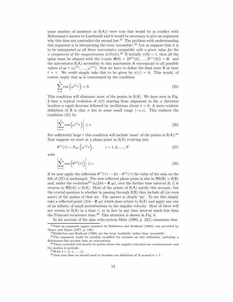
If we now apply the reflection θ(i)(τ) → 2π− θ(i)(τ) the value of the sum on theleft of (27) is unchanged. The new reflected phase point is also in RS(B) ≡ S(B)and, under the evolution25 φt(2πi−θ, ω), over the further time interval [0, τ ] itreturns to RS(A) ≡ S(A). Most of the points of S(A) satisfy this account, butthe crucial question is whether in passing through S(B) they include all (or evenmost) of the points of that set. The answer is clearly ‘no’. To see this simplytake a reflected point (2πi−θ, ω) which does return to S(A) and apply any oneof an infinity of small perturbations to the angular velocity. Most of these willnot return to S(A) in a time τ , or in fact in any time interval much less thanthe Poincare recurrence time.26 This situation is shown in Fig. 6.

In his account of the spin–echo system Sklar (1993, p. 221) comments that21Such an argument (again repeated by Ridderbos and Redhead (1998)) was provided by

Mayer and Mayer (1977, p. 136).22Ridderbos and Redhead (1998) use the term ‘available’ rather than ‘accessible’.23The argument could be suitably modified for variants on this definition, including a

Boltzmann-like account base on macrostates.24Those excluded will mostly be points where the angular velocities are commensurate and

the motion is periodic.25With i = (1, 1, . . . , 1).26And even then we should need to broaden our definition of A around σ = 1.

13

σ

t

–0.2

0

0.2

0.4

0.6

0.8

1

20 40 60 80 100 120 140 160 180 200

Figure 6: The evolution of the magnetization density. After t = 100 the systemis reflected and the angular velocities are subject to small perturbations.

“It is as if we could prepare a gas in such a way that an ensembleof gases so prepared would initially be uniformly spread throughouta box. But the overwhelming majority of the gases in the ensemblewould then spontaneously flow to the left-hand half of the box.”

The problematic word in this quote is ‘prepare’. To prepare ‘from scratch’ aspin system or any other assembly is such a way that it will achieve a particularmacrostate (low entropy, high magnetization, etc.) after a particular intervalof time would involve careful adjustment of the relationships of velocities andpositions for each microsystem; a task worthy of a Maxwell demon. However,what we have here is a much simpler process. We allow the system to achievevalues which imply a recent memory of the required macrostate and then applya reflection. This macroscopic operation by a Loschmidt demon27 is only partof the process of preparation. The difficult part is left to the system.

The aim of the work of Ridderbos and Redhead (1998) is to use an ex-amination of the spin–echo system to discredit the use of the Gibbs-Ehrenfestcoarse-graining in favour of an interventionist approach. While it is true thatthe status of the coarse-grained Gibbs entropy lacks the clarity of the Boltzmannentropy it is by no means clear that the criticisms levelled at this approach byRidderbos and Redhead (1998) are all valid. In Sec. 1.1.2 we described twomethods for following the evolution of the coarse-grained Gibbs entropy, thefirst, involving a coarse-graining of the fine-grained distribution at each instantof time, and the second a sequence of re-coarse-graining as time progresses.The former, which is the standard understanding of the procedure (Denbighand Denbigh, 1985, p. 55), does not yield a strict monotonic increase of en-tropy. However, it does allow the system to retrace its steps, either by velocityreversal or reflection(see Fig. 5). This is in conflict with the remarks of Ridder-bos and Redhead (1998, p. 1250) that a “reversal of the dynamical evolutionin the coarse-grained case does not cause the distribution to evolve back to itsoriginal form”. They appear to be thinking of the (obvious) impossibility of

27The term Loschmidt demon, seems to have been introduced by Rhim et al. (1971).

14

un-coarse-graining a coarse-grained distribution. The occurrence of the echo inthese circumstances would certainly be “completely miraculous” (ibid, p. 1251),but this is not how coarse-grained evolution should be implemented. In anyevent, the more important question, raised by Ridderbos and Redhead (1998,p. 1251), is whether the spin–echo system is a “counterexample to the secondlaw of thermodynamics”. The answer to this is surely that it depends on whatyou mean by the second law of thermodynamics. If, along with Maxwell andBoltzmann and probably the majority of physicists (see e.g. Ruelle, 1991, p.113) entropy increase in an isolated system is taken to be highly probable butnot certain, then the spin–echo model, along with simulations of other simplemodels (Lavis, 2003), is a nice example of the workings of the law. However,if entropy increase is an iron certainty this example is one, and not a special,example of a violation of the second law. Ridderbos and Redhead (1998, p.1251) assert that the spin–echo experiments are not a violation of the secondlaw because “we do not have a situation where a system evolves spontaneouslyfrom a high entropy state to a low entropy state.” Apart from the obviousconflict with the quote from Sklar given above, this, of course, depends on whatyou mean by “spontaneous”. Any experiment or simulation involves preparingthe system in some initial state from which it evolves spontaneously. There is noconceptual reason why the system cannot be prepared in a state from which theentropy spontaneously decreases. It just difficult to do because of their relativepaucity. As we have already indicated in our discussion the best way to findsuch a state is to let the system find it itself by evolving in the reverse direction.Then restarting the system in this state it will show a ‘spontaneous’ decrease inentropy.

4 Conclusions

We have considered the case made for the spin–echo experiments being an ex-ample of a special system which destroys the argument for using coarse-graining.We have argued that the reason for the Boltzmann version of coarse-graininghas nothing to do with the inability to do fine-grained dynamic calculations,28

or experiments, but is based on the necessity to have a demarkation between themicro- and macro-scales. The same arguments apply to Gibbs-Ehrenfest coarse-graining. The spin–echo experiments are of technical significance, particularlyin respect of the fact that the echoing procedure can be effected by macroscopicmeans, but as a theoretical model of an assembly of non-interacting microsys-tems it is in no way special, as we have shown elsewhere (Lavis, 2003).

References

Baxter, R. J. (1982). Exactly Solved Models in Statistical Mechanics, AcademicPress.

Blatt, J. M. (1959). An alternative approach to the ergodic problem, Prog. Th.Phys. 22: 745–756.

28Indeed to calculate the Boltzmann entropy one needs the dynamic detail.

15

Boltzmann, L. (1877). On the relation of a general mechanical theorem to thesecond law of thermodynamics, in S. G. Brush (ed.), Kinetic Theory, Vol.2 (1966), Pergamon, pp. 188–193. English Reprint.

Brewer, R. G. and Hahn, E. L. (1984). Atomic memory, Scientific American251(6): 36–50.

Denbigh, K. G. and Denbigh, J. S. (1985). Entropy in Relation to IncompleteKnowledge, Cambridge U. P.

Ehrenfest, P. and Ehrenfest-Afanassjewa, T. (1912). The Conceptual Founda-tions of the Statistical Approach in Mechanics, English translation, CornellU. P.

Gibbs, J. W. (1902). Elementary Principles in Statistical Mechanics, Yale U. P.Reprinted by Dover Publications, 1960.

Grunbaum, A. (1975). Is the coarse-grained entropy of classical statistical me-chanics an anthropomorphism?, in L. Kubat and J. Zeman (eds), Entropyand Information in Science and Philosophy, Elsevier, pp. 173–186.

Hahn, E. L. (1950). Spin echoes, Phys. Rev. 80: 580–594.

Hahn, E. L. (1953). Free nuclar induction, Physics Today 6(11): 4–9.

Landau, L. D. and Lifshitz, E. M. (1959). Fluid Mechanics, Pergamon.

Lavis, D. A. (2003). Some examples of simple systems: Version 2.www.mth.kcl.ac.uk/∼dlavis/papers/examples-ver2.pdf.

Lebowitz, J. L. (1993). Boltzmann’s entropy and time’s arrow, Physics Today46: 32–38.

Loschmidt, J. (1876). Uber den Zustand des Warmegleichgewichtes eines Sys-tems von Korpern mit Rucksicht auf die Schwerkraft, Wiener Berichte73: 139.

Mayer, J. E. and Mayer, M. G. (1977). Statistical Mechanics, Wiley.

Poincare, H. (1890). On the three-body problem and the equations of dynamics,in S. G. Brush (ed.), Kinetic Theory, Vol. 2 (1966), Pergamon, pp. 194–202. English Reprint.

Rhim, W.-K., Pines, A. and Waugh, J. S. (1971). Time-reversal experiments indipolar–coupled spin systems, Phys. Rev. B 3: 684–696.

Ridderbos, K. (2002). The course-graining approach to statistical mechanics:how blissful is our ignorance?, Stud. Hist. Phil. Mod. Phys. 33: 65–77.

Ridderbos, T. M. and Redhead, M. L. G. (1998). The spin-echo experiments andthe second law of thermodynamics, Foundations of Physics 28: 1237–1270.

Ruelle, D. (1991). Chance and Chaos, Princeton U. P.

Sklar, L. (1993). Physics and Chance, Cambridge U. P.

Tolman, R. C. (1938). The Principles of Statistical Mechanics, Oxford U. P.

16